r. schreier analog devices, inc. snr calculation and spectral estimation...

R. SCHREIER ANALOG DEVICES, INC.

1

SNR Calculation andSpectral Estimation[S&T Appendix A]

or, How not to make a mess of an FFT

0 Make sure the input is located in an FFT bin1 Window the data!

A Hann window works well.

2 Compute the FFT3 SNR = power in signal bins / power in noise bins4 If you want to make a spectral plot

i. Apply sine-wave scalingii. State the noise bandwidth (NBW)iii. Smooth the FFT

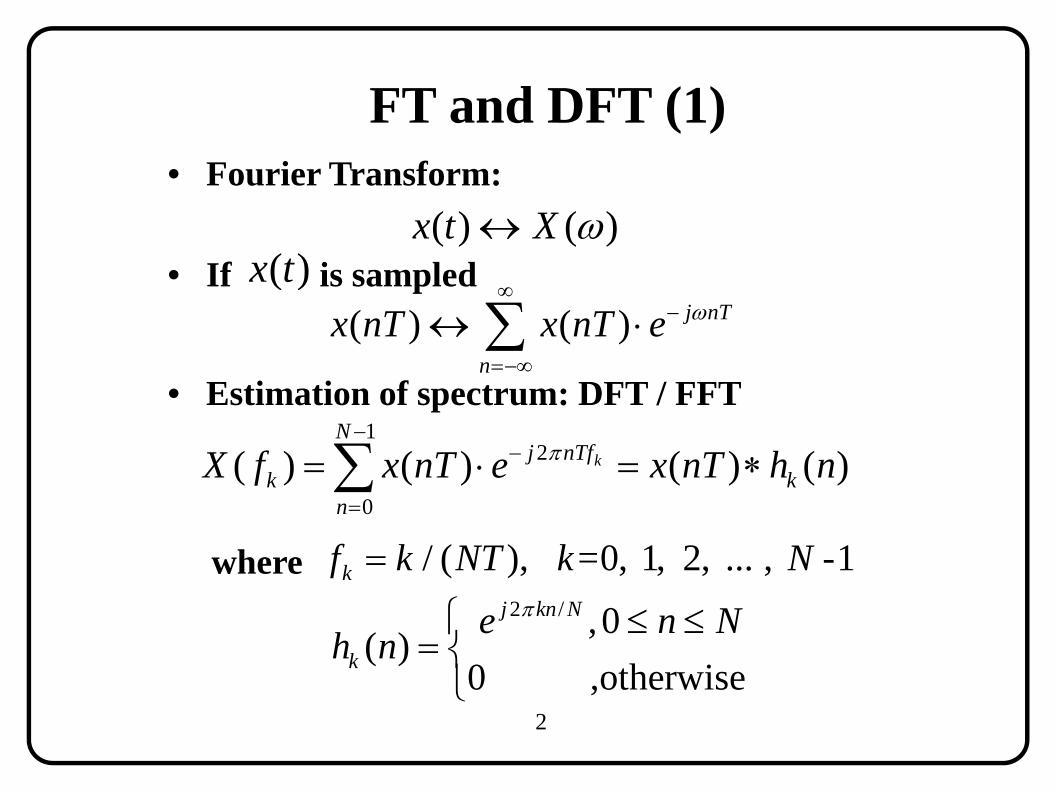
FT d DFT (1)FT and DFT (1)• Fourier Transform:• Fourier Transform:

If i l d( ) ( )x t X

( )x t• If is sampled( )x t( ) ( ) j nTx nT x nT e

• Estimation of spectrum: DFT / FFTn

1N2

0( ) ( ) ( ) ( )kj nTf

k kn

X f x nT e x nT h n

where / ( ), =0, 1, 2, ... , -1 kf k NT k N

2 / 0j kn N N 2 / ,0( )

0 ,otherwise

j kn N

ke n N

h n

2

FT d DFT (2)FT and DFT (2)

• Generally, in Fourier Transformation, therule isrule is

Sampled Periodic Sampled Periodic

• If is not periodic with period NT, theDFT calculates the spectrum of a discontinuous

( )x nT

signal -- bad estimate!

3

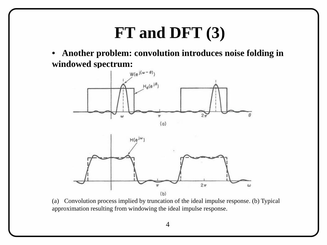
FT d DFT (3)FT and DFT (3)• Another problem: convolution introduces noise folding inAnother problem: convolution introduces noise folding inwindowed spectrum:

(a) Convolution process implied by truncation of the ideal impulse response. (b) Typicalapproximation resulting from windowing the ideal impulse response.

4

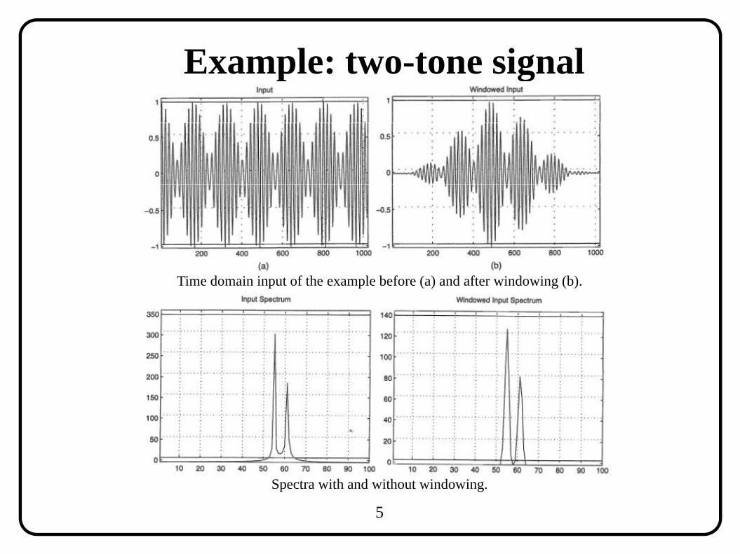
Example: two tone signalExample: two-tone signal

Time domain input of the example before (a) and after windowing (b).

Spectra with and without windowing.

5

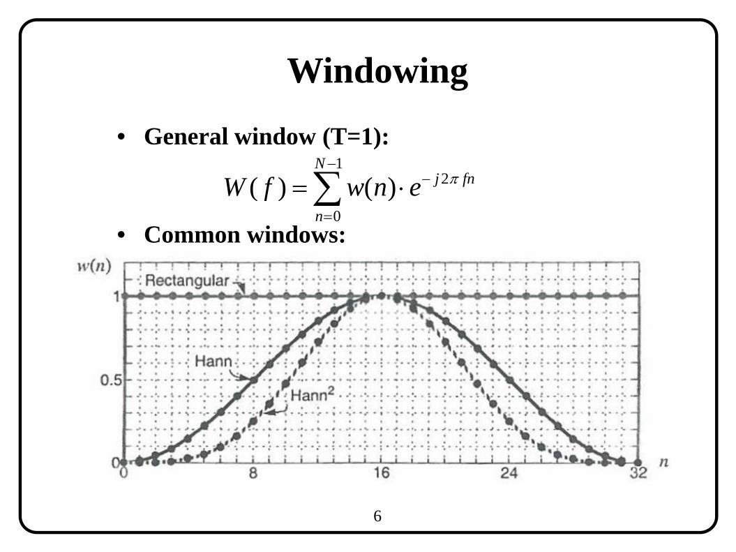
Wi d iWindowing

• General window (T=1):1

2( ) ( )N

j fnW f w n e

• Common windows:

0( ) ( ) j f

nW f w n e

6


7

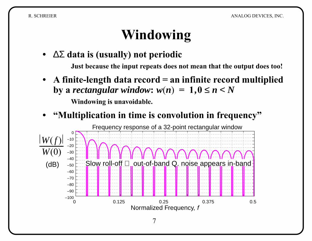
Windowing• ∆Σ data is (usually) not periodic

Just because the input repeats does not mean that the output does too!

• A finite-length data record = an infinite record multipliedby a rectangular window: ,

Windowing is unavoidable.

• “Multiplication in time is convolution in frequency”

w n( ) 1= 0 n≤ N<

0 0.125 0.25 0.375 0.5–100

–90

–80

–70

–60

–50

–40

–30

–20

–10

0

Normalized Frequency, f

(dB)

Frequency response of a 32-point rectangular window

Slow roll-off ⇒ out-of-band Q. noise appears in-band

W f( )W 0( )

---------------


8

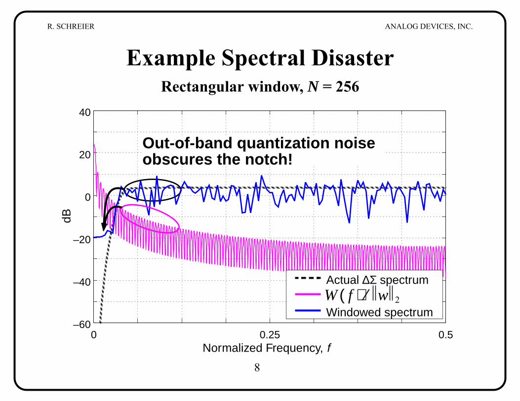
Example Spectral DisasterRectangular window, N = 256

0 0.25 0.5–60

–40

–20

0

20

40


dB

Actual ∆Σ spectrum

Windowed spectrumW f( ) w 2⁄

Out-of-band quantization noiseobscures the notch!


9

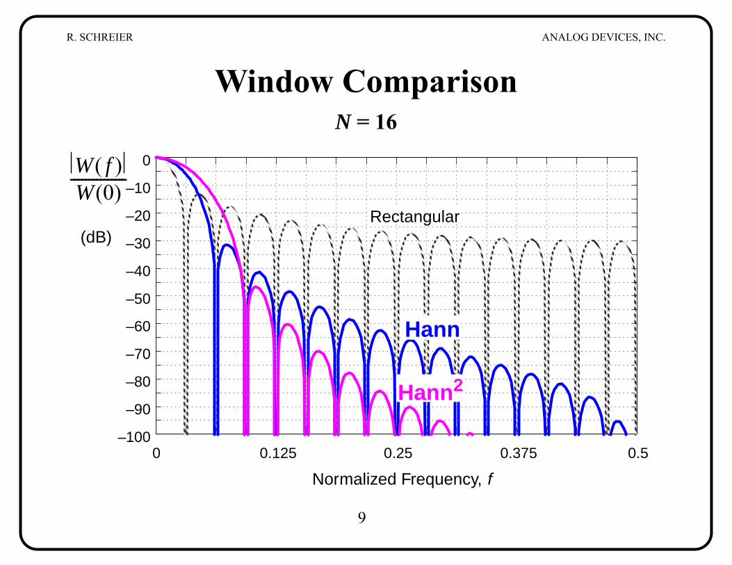
Window ComparisonN = 16

0 0.125 0.25 0.375 0.5–100

–90

–80

–70

–60

–50

–40

–30

–20

–10

0


(dB)Rectangular

W f( )W 0( )

---------------

Hann2

Hann


10

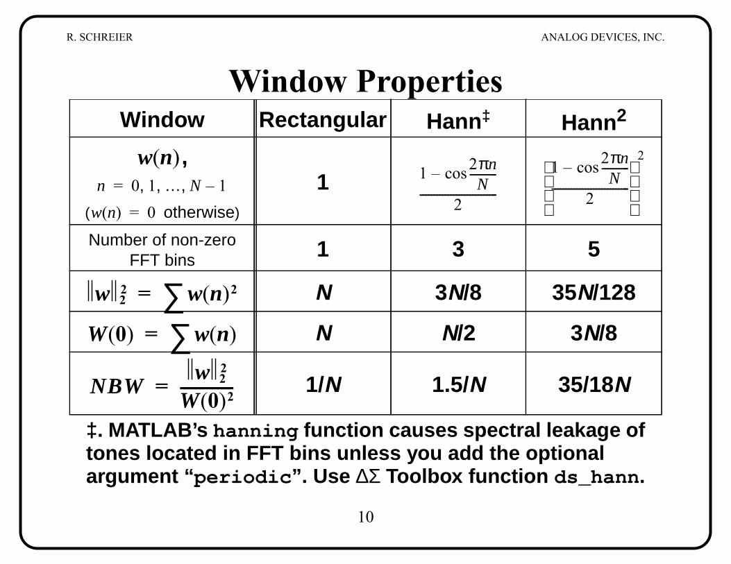
Window PropertiesWindow Rectangular Hann‡

‡. MATLAB’s hanning function causes spectral leakage oftones located in FFT bins unless you add the optionalargument “periodic”. Use ∆Σ Toolbox function ds_hann.

Hann2

,

( otherwise)

1

Number of non-zeroFFT bins 1 3 5

N 3N/8 35N/128

N N/2 3N/8

1/N 1.5/N 35/18N

w n( )n 0 1 … N 1–, , ,=

w n( ) 0=

1 2πnN

----------cos–

2----------------------------

1 2πnN

----------cos–

2----------------------------

2

w 22 w n( )2∑=

W 0( ) w n( )∑=

NBWw 2

2

W 0( )2--------------=


11

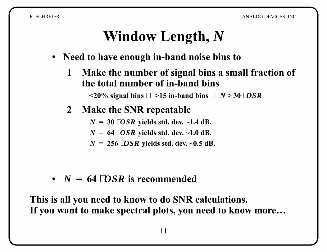
Window Length, N• Need to have enough in-band noise bins to

1 Make the number of signal bins a small fraction ofthe total number of in-band bins

<20% signal bins ⇒ >15 in-band bins ⇒

2 Make the SNR repeatable yields std. dev. ~1.4 dB. yields std. dev. ~1.0 dB. yields std. dev. ~0.5 dB.

• is recommended

This is all you need to know to do SNR calculations.If you want to make spectral plots, you need to know more…

N 30 OSR⋅>

N 30 OSR⋅=N 64 OSR⋅=N 256 OSR⋅=

N 64 OSR⋅=


12

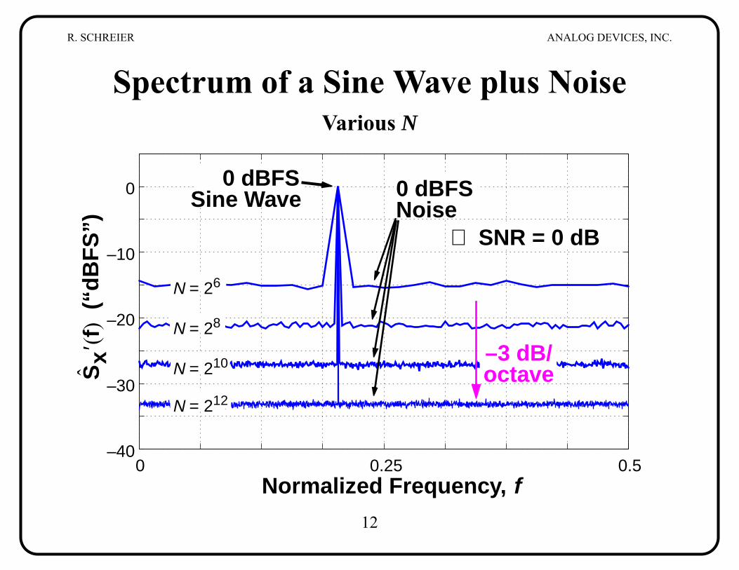
Spectrum of a Sine Wave plus NoiseVarious N


(“dB

FS

”)S

x′f(

)

0 0.25 0.5–40

–30

–20

–10

0

N = 26

N = 28

N = 210

N = 212

0 dBFS 0 dBFSSine Wave Noise

–3 dB/octave

⇒ SNR = 0 dB


13

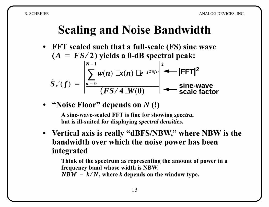
Scaling and Noise Bandwidth• FFT scaled such that a full-scale (FS) sine wave

( ) yields a 0-dB spectral peak:

• “Noise Floor” depends on N (!)A sine-wave-scaled FFT is fine for showing spectra,but is ill-suited for displaying spectral densities.

• Vertical axis is really “dBFS/NBW,” where NBW is thebandwidth over which the noise power has beenintegrated

Think of the spectrum as representing the amount of power in afrequency band whose width is NBW.

, where k depends on the window type.

A FS 2⁄=

Sx′ f( )w n( ) x n( ) e j2πfn–⋅ ⋅

n 0=

N 1–

∑FS 4⁄( )W 0( )-----------------------------------------------------

2

=|FFT|2

sine-wavescale factor

NBW k N⁄=


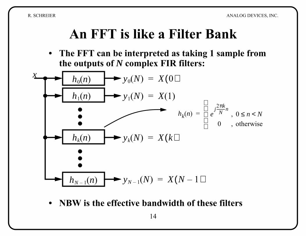
An FFT is l Filter Bank• The FFT can be int as taking 1 sample from

the outputs of N com R filters:

• NBW is the effectiv

x h0 n( )

h1 n( )

hk n( )

hN 1– n( )

y0 N( 0)

y1 N( 1)

yk N(

yN –

hk n( ) ej2πkN

---------n, 0 n N<≤

=

ike a erpreted

plex FI) X(=

) X(=

14

e bandwidth of these filters

) X k( )=

1 N( ) X N 1–( )=

0 , otherwise


15

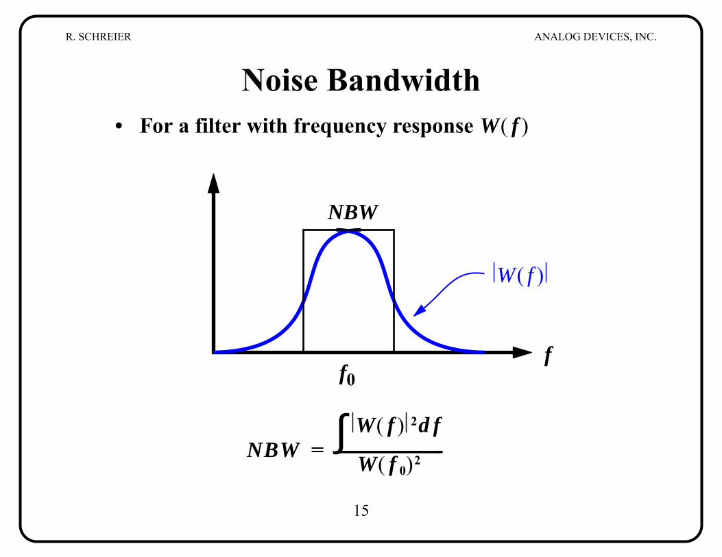
Noise Bandwidth• For a filter with frequency response W f( )

NBWW f( ) 2 fd∫W f 0( )2-----------------------------=

f

NBW

f0

W f( )


16

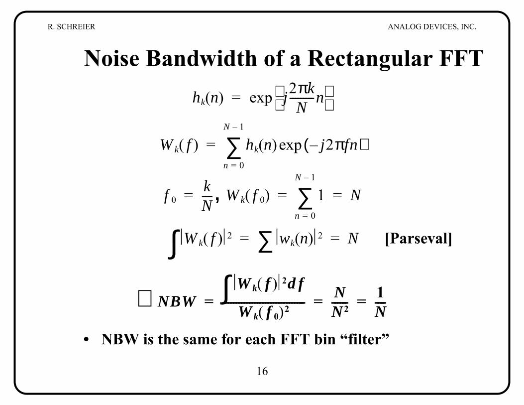
Noise Bandwidth of a Rectangular FFT

,

[Parseval]

∴• NBW is the same for each FFT bin “filter”

hk n( ) j2πkN

---------n exp=

Wk f( ) hk n( ) j– 2πfn( )expn 0=

N 1–

∑=

f 0kN----= Wk f 0( ) 1

n 0=

N 1–

∑ N= =

Wk f( ) 2∫ wk n( ) 2∑ N= =

NBWWk f( ) 2 fd∫Wk f 0( )2------------------------------- N

N2------ 1N----= = =


17

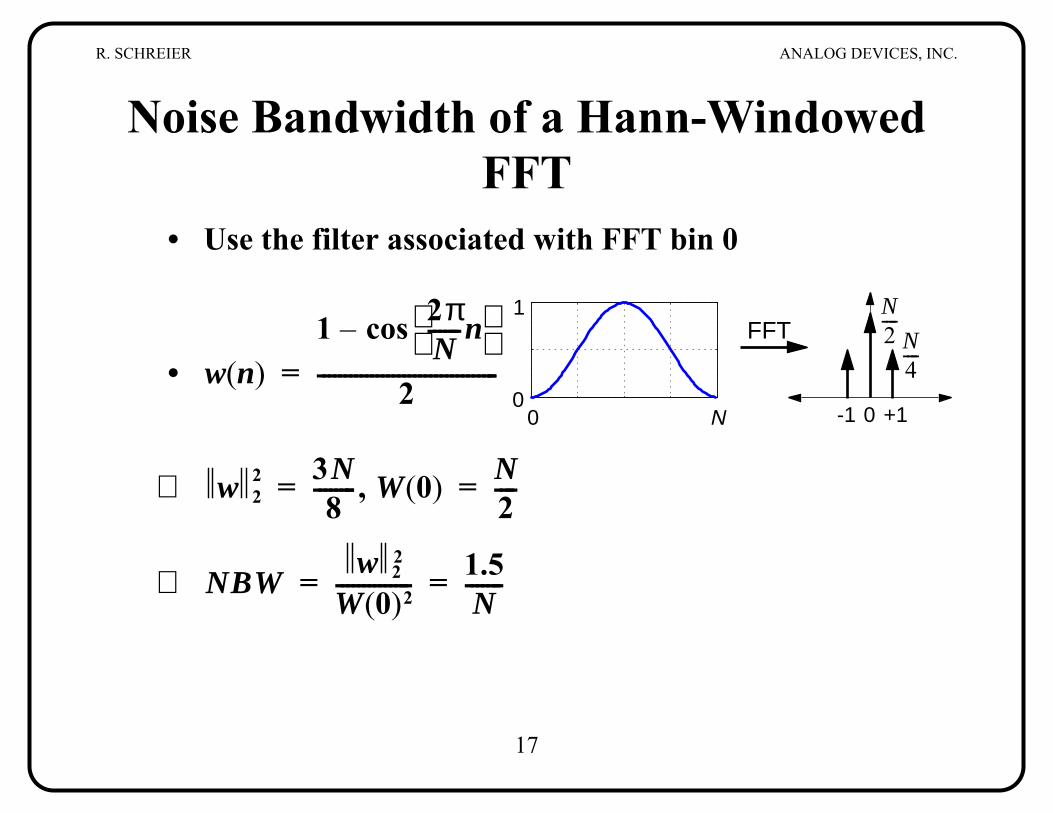
Noise Bandwidth of a Hann-WindowedFFT

• Use the filter associated with FFT bin 0

•

⇒ ,

⇒

w n( )1 2π

N------n

cos–

2----------------------------------=0 N

0

1

0 +1-1

N2----

N4----

FFT

w 22 3N

8--------= W 0( ) N2----=

NBWw 2

2

W 0( )2-------------- 1.5N

-------= =


18

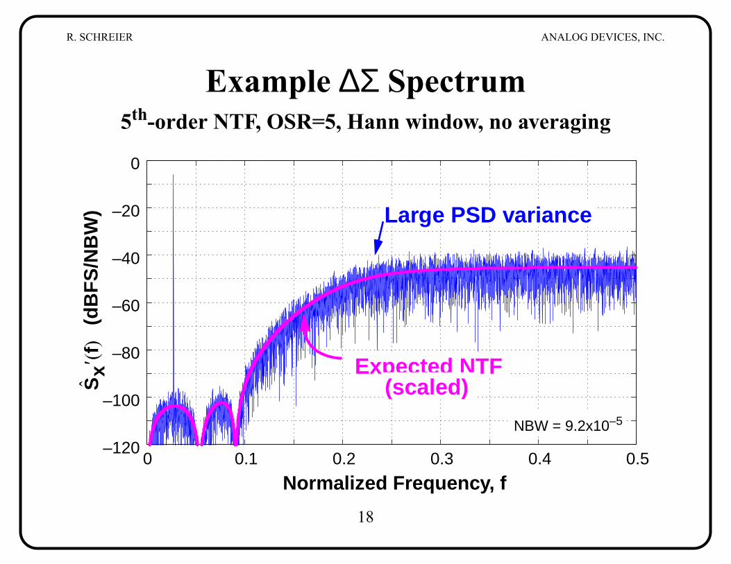
Example ∆Σ Spectrum5th-order NTF, OSR=5, Hann window, no averaging

0 0.1 0.2 0.3 0.4 0.5–120

–100

–80

–60

–40

–20

0


(dB

FS

/NB

W)

Sx

′f()

NBW = 9.2x10–5

Large PSD variance

Expected NTF(scaled)


19

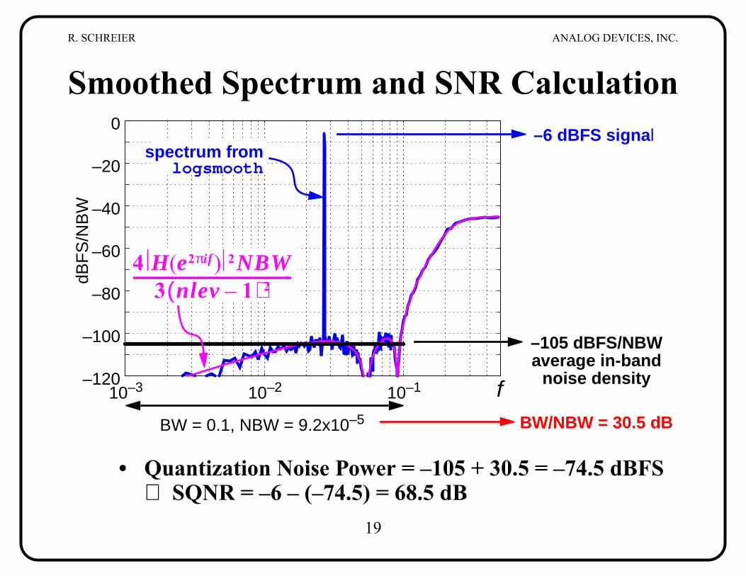
Smoothed Spectrum and SNR Calculation

• Quantization Noise Power = –105 + 30.5 = –74.5 dBFS⇒ SQNR = –6 – (–74.5) = 68.5 dB

10–3 10–2 10–1–120

–100

–80

–60

–40

–20

0

dBF

S/N

BW

4 H e2πif( ) 2NBW3 nlev 1–( )2------------------------------------------

spectrum fromlogsmooth

–6 dBFS signal

–105 dBFS/NBWaverage in-band

fBW/NBW = 30.5 dB

noise density

BW = 0.1, NBW = 9.2x10–5


20

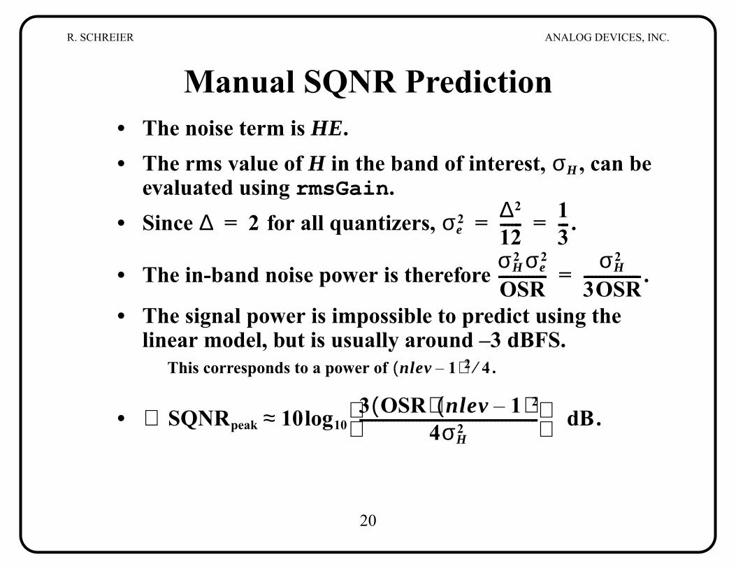
Manual SQNR Prediction• The noise term is HE.• The rms value of H in the band of interest, , can be

evaluated using rmsGain.• Since for all quantizers, .

• The in-band noise power is therefore .

• The signal power is impossible to predict using thelinear model, but is usually around –3 dBFS.

This corresponds to a power of .

• .

σH

∆ 2= σe2 ∆2

12------ 13---= =

σH2 σe

2

OSR------------- σH2

3OSR---------------=

nlev 1–( )2 4⁄

SQNRpeak∴ 10log103 OSR( ) nlev 1–( )2

4σH2------------------------------------------------

dB≈

r. schreier analog devices, inc. snr calculation and spectral estimation...

Documents