ECE1371 Advanced Analog CircuitsLecture 4

EXAMPLE DESIGN– PART 2

Richard Schreierrichard.schreier@analog.com

Trevor Caldwelltrevor.caldwell@utoronto.ca

ECE1371 4-2

Course Goals

• Deepen understanding of CMOS analog circuitdesign through a top-down study of a modernanalog system— a delta-sigma ADC

• Develop circuit insight through brief peeks atsome nifty little circuits

The circuit world is filled with many little gems thatevery competent designer ought to know.

ECE1371 4-3

Date Lecture (M 13:00-15:00) Ref Homework

2015-01-05 RS 1 MOD1 & MOD2 ST 2, 3, A 1: Matlab MOD1&2

2015-01-12 RS 2 MODN + ∆Σ Toolbox ST 4, B 2: ∆Σ Toolbox

2015-01-19 RS 3 Example Design: Part 1 ST 9.1, CCJM 14 3: Sw.-level MOD2

2015-01-26 RS 4 Example Design: Part 2 CCJM 18

2015-02-02 TC 5 SC Circuits R 12, CCJM 14 4: SC Integrator

2015-02-09 TC 6 Amplifier Design

2015-02-16 Reading Week– No Lecture

2015-02-23 TC 7 Amplifier Design 5: SC Int w/ Amp

2015-03-02 RS 8 Comparator & Flash ADC CCJM 10

Project

2015-03-09 TC 9 Noise in SC Circuits ST C

2015-03-16 RS 10 Advanced ∆Σ ST 6.6, 9.4

2015-03-23 TC 11 Matching & MM-Shaping ST 6.3-6.5, +

2015-03-30 TC 12 Pipeline and SAR ADCs CCJM 15, 17

2015-04-06 Exam Proj. Report Due Friday April 10

2015-04-13 Project Presentation

ECE1371 4-4

NLCOTD: Non-Overlapping ClockGenerator

• Our SC circuits require two non-overlappingclocks. How do we generate them?

?

ECE1371 4-5

Highlights(i.e. What you will learn today)

1 Transistor-level implementation of MOD2op-amp, SC CMFB, comparator, clock generator

2 MOD2 variants

3 Variable quantizer gain

ECE1371 4-6

Review: MOD2Standard Block Diagram

Scaled Block Diagram

Q1z−1

zz−1

U VE

NTF z( ) 1 z 1––( )2=STF z( ) z 1–=

Q1z−1

zz−1

U V

1/91/3

1/3 1/3 9X1’ X2’

ECE1371 4-7

Review: Schematic

• 1st-stage capacitor sizes set for SNR = 100 dB@ OSR = 500 and –3-dBFS input

Vref = 1V and the full-scale input range is ±1 V.

• 2nd-stage capacitor sizes set by minimumallowable capacitance

ECE1371 4-8

Review: Simulated Spectrum

–140

–120

–100

–80

–60

–40

–20

0

Theoretical PSD(k = 1)

Frequency (Hz)

dBF

S/N

BW

NBW = 46 Hz

SQNR = 105 dB@ OSR = 500

100 1k 10k 100k

Smoothed Spectrum

3rd harmonic–108-dBc

ECE1371 4-9

Review: Implementation Summary1 Choose a viable SC topology and manually

verify timing

2 Do dynamic-range scalingYou now have a set of capacitor ratios.Verify operation.

3 Determine absolute capacitor sizesVerify noise.

4 Determine op-amp specs and construct atransistor-level schematic

Verify.

5 Layout, fab, debug, document, get customers,sell by the millions, go public, …

ECE1371 4-10

Effect of Finite Op Amp GainLinear Theory

• Suppose that the amplifier has finite DC gain A.Define .

• To determine the effect on the integrator pole,let’s look at our SC integrator with zero input:

µ 1 A⁄=

C1φ1

C2

φ1

φ2

φ2 v q 2 C2⁄=

µq 2 C2⁄–

A

µC1 C2⁄( )q 2

ECE1371 4-11

• A fraction of q2 leaks away each clock cycle:

,

where

• Thus, the integrator is lossy, with a pole at

Q: How big can ε get before the effect becomessignificant?

q 2 n 1+( ) 1 ε–( )q 2 n( )=

ε µC1 C2⁄=

z 1 ε–=

π OSR⁄

ε A: ε π OSR⁄≈

z-plane:

z = 1

ECE1371 4-12

Op Amp Gain RequirementLinear Theory

• According to the linear theory, finite op amp gainshould not degrade the noise significantly aslong as

• For our implementation of MOD2, in which and , this leads to

,which is quite a lax requirement!

• As OSR is decreased, the gain requirement goesdown

A C 1 C2⁄( ) OSR π⁄( )>

C1 C2⁄ 1 4⁄= OSR 500=A 40> 32 dB=

ECE1371 4-13

Op Amp TransconductanceSettling time

• Model the op amp as a simple gm:

• This is a single-time-constant-circuit with

C1

C2

C3gm

Ceff

β

gmvv

β C2 C1 C2+( )⁄=Ceff C3 C1C2 C1 C2+( )⁄+=

1βg m-----------

τ Ceff βg m( )⁄=

ECE1371 4-14

Settling Requirements• If gm is linear, incomplete settling has the same

effect as a coefficient error and thus gm can bevery low

• In practice, the gm is not linear and we need toensure nearly complete settling

• As a worst case scenario, let’s require transientsto settle to 1 part in 10 5

This should be more than enough for –100 dBcdistortion.

ECE1371 4-15

Settling Requirements (cont’d)• If linear settling is allocated 1/4 of a clock period,

we want , or τ = ns

and thus

• For INT1 of our MOD2:

*

MHz⇒ µA/V

*. 0.5 comes from the single-ended to differential translation.

T 4⁄τ

-----------– exp 10 5–= T

4 105ln------------------- 20=

g mCeff

βτ-----------

Ceff

β-----------4f s 105ln= =

Ceff 0.5 4p 1.33p⋅4p 1.33p+----------------------------- 30f+

0.5 pF= =

β 3 4⁄=f s 1=

g m 30=

ECE1371 4-16

Slewing• The maximum charge transferred through C1 is

• If we require the slew current to be enough totransfer qmax in 1/4 of a clock period, then

µA

C1up,max = 0.5 V

vrefn = –0.5 Vq max C1 1V⋅ 1.33 pC= =

I slewq max

T 4⁄------------ 5≈=

ECE1371 4-17

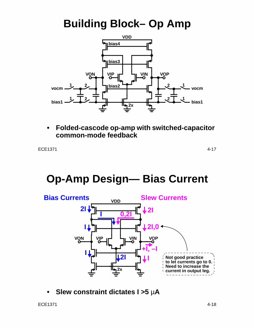
Building Block– Op Amp

• Folded-cascode op-amp with switched-capacitorcommon-mode feedback

VDD

2xbias1

1

1

2

2

vocm

bias1

1

1

2

2

vocmbias2

bias3

bias4

VIP VINVON VOP

ECE1371 4-18

Op-Amp Design— Bias Current

• Slew constraint dictates I >5 µA

VDD

2x

VIP VINVON VOP

2I

2I

I

I

I

Bias Currents Slew Currents

2I,0

2I

I

0,2I

+I, –INot good practiceto let currents go to 0.Need to increase thecurrent in output leg.

ECE1371 4-19

Op-Amp Design— gm

• Square-law MOSFET model:

• µA, µA/V ⇒ VUsually mV, so we should be able to gethigh enough gm.

v gmv+v

2--- –v

2---

I = gm1v/2

M1

∴ gm = 0.5 gm1

g m1 2I D( ) ∆V( )⁄=

I D 5= g m 30≥ ∆V 0.33≤∆V 200≈

ECE1371 4-20

Transistor Sizes & Bias Point

• Allowable swing is +0.6 V, –0.75 V

• Simulated gm = 36 µA/V, A = 48 dBgm is high enough and the gain is 6 × required.

2.5V

0.5/0.3

2.5/0.3

2.5/0.6

0.75/0.3

0.75/0.61.0/0.6

12.5µA

7.5µA

10µA

W/L

Vdsat =0.15V

Vdsat =0.15V

0.35V

2.0V

1.25V

ECE1371 4-21

Ideal Common-Mode Feedback

• Can use this circuit to speed up the simulation

OP

ONOP–CM

ON–CM

ECE1371 4-22

Simulated WaveformsP2V

.2

.4

.6

.8

1

1.2

1.4

1.6

1.8

2

2.2

0.5 µs/div

v(x1p)

v(x1n) The output voltage initially goes the wrong way?

ECE1371 4-23

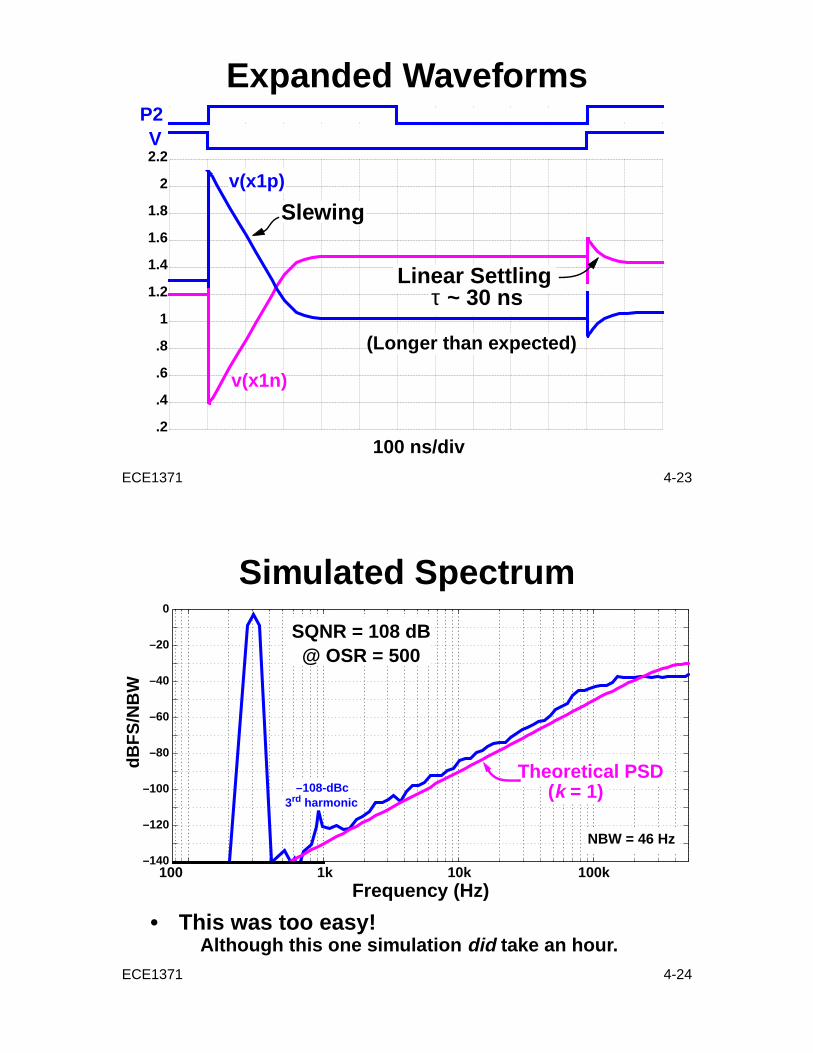
Expanded WaveformsP2V

100 ns/div

.4

.6

.8

1

1.2

1.4

1.6

1.8

2

2.2

Slewing

Linear Settlingτ ~ 30 ns

.2

v(x1p)

v(x1n)

(Longer than expected)

ECE1371 4-24

Simulated Spectrum

• This was too easy!Although this one simulation did take an hour.

Frequency (Hz)

dBF

S/N

BW

100 1k 10k 100k–140

–120

–100

–80

–60

–40

–20

0

Theoretical PSD(k = 1)

NBW = 46 Hz

SQNR = 108 dB@ OSR = 500

3rd harmonic–108-dBc

ECE1371 4-25

SC Common-Mode FeedbackCommon-Mode 1/2-Circuit

• Vocm = Vcm + Vgs1 – V1If V1 = Vgs1, then Vocm = Vcm.

VcmV1

Vcm–V1Ca Cb

Vgs1

M1

Vocm

I

ECE1371 4-26

Latched Comparator

• Falling phase 1 initiates regenerative actionS and R connected to a Set/Reset latch.

VDD

1

VSS

1 1

Y+ Y–

SR

S

R

v

Inverter thresholds are chosenso that the inverters respondonly after R/S have resolved.

Set/Reset Latch:

ECE1371 4-27

Switch ResistanceSampling Phase

• If Rsw is constant, its has only a filtering (linear)effect, which is benign

• Unfortunately, the on-resistance of MOSswitches varies with V gs (and hence V in)

⇒ Must make MOS switches large enough

Rsw

C1

Vin

ECE1371 4-28

Switch ResistanceIntegration Phase

• Rsw increases the settling time by a factor of1 + 4gmRsw

⇒ Set to make the increase in τ small

• So in our MOD2, we want Rsw ≤ 0.75 kΩ.BTW, my simulation used k Ω and was OK.

C1

C2

2gm

RswDifferentialHalf-Circuit:

Rsw1

40g m---------------≤

Rsw 1=

ECE1371 4-29

NLCOTD: Non-Overlapping ClockGenerator

?CK

P1

P2

ECE1371 4-30

Non-Overlapping Clock Generator

• Non-overlap time set by NOR’s tPLH

CK P1

P2

CK

P1

P2

ECE1371 4-31

Clocking Details—Early/Late Phases

• Charge injected via M1 is (non-linearly) signal-dependent, whereas charge injection from M2 issignal-independent

⇒ Open M2 (early) then open M1 (late) so thatcharge injected from C gs1 cannot enter C1

1

1D

1D1

M1M2

C1

ECE1371 4-32

Clocking Details—Bottom-plate sampling

• Parasitic capacitance on the right terminal of C1degrades the effectiveness of early/late clocking

• Cp for the top plate is smaller, so use the topplate for the right terminal and the bottom platefor the left

1

1D

M1M2

C1

Cp

SubstrateBottom

Plate

small big

ECE1371 4-33

Complementary Clock Alignment• We need complementary clocks if transmission

gates are used for the switches

Q: How do we align them?

A: Carefully size the inverters relative to theircapacitive loads, or use a transmission gate tomimic an inverter delay:

CK CKP

CKN

CK CKP

CKNNeed to match delayof 3 INVs to 2 INVs

ECE1371 4-34

Professional Clock Generator

• To maximize the time available for settling, makethe early and late phases start at the same time

**

**

CK

1

2D

1D

2Delay

CK

1

1D

2

2D

Buffers fordriving largeclock loads

Non-overlapcontrol

control

ECE1371 4-35

Review: Implementation Summary1 Choose a viable SC topology and manually

verify timing

2 Do dynamic-range scaling

3 Determine absolute capacitor sizes

4 Determine op-amp specs and construct atransistor-level schematic

Verify. Verify. Verify.

5 Layout, fab, debug, document, get customers,sell by the millions, go public, …

This last step is an “exercise for the reader.”

ECE1371 4-36

Topological Variant–Feed-Forward

+ Output of first integrator has no DC componentDynamic range requirements of this integrator arerelaxed.

– Although near , for

Instability is more likely.

Qzz−1

1z−1

U VE

STF z( ) 2z 1– z 2––=NTF z( ) 1 z 1––( )2=

STF 1≈ ω 0=STF 3= ω π=

ECE1371 4-37

Topological Variant–Feed-Forward with Extra Feed-In

+ No DC component in either integrator’s outputReduced dynamic range requirements in bothintegrators, esp. for multi-bit modulators.

+ Perfectly flat STFNo increased risk of instability.

– Timing is tricky

Qzz−1

1z−1

U VE

STF z( ) 1=NTF z( ) 1 z 1––( )2=

ECE1371 4-38

Topological Variant–Error Feedback

+ Simple

– Very sensitive to gain errorsOnly suitable for digital implementations.

QU VE

NTF z( ) 1 z 1––( )2=STF z( ) 1=

z-1z-1

2–E

ECE1371 4-39

Is MOD2The Only 2 nd-Order Modulator?• Except for the filtering provided by the STF, any

modulator with the same NTF as MOD2 has thesame input-output behavior as MOD2

SQNR curve is the same.Tonality of the quantization noise is unchanged.

• Internal states, sensitivity, thermal noise etc. candiffer from realization to realization

BUT, in terms of input-output behavior,

• A 2nd-order modulator is truly different only if itpossesses a truly different (2 nd-order) NTF

ECE1371 4-40

A Better 2 nd-Order NTF

-1 0 1-1

0

1Pole-Zero Plot

Moving polescloser to zeroslowers NTF gain,

Separating thezeros reducesin-band noise:

-fB fBa-a

2

allowing largerinputs

ECE1371 4-41

NTF Comparison

10–4 10–3 10–2 10–1–100

–80

–60

–40

–20

0

20

Normalized Frequency

Plain MOD2Improved MOD2

NTF zeronear passband

edge

4 dB lowerNTF gaindB

ECE1371 4-42

SNR vs. Amp Comparison

–100 –80 –60 –40 –20 00

20

40

60

80

100

120

Signal Amplitude (dBFS)

SQ

NR

(dB

)

MOD2MOD2b

~ 6 dB better

MOD2b more tolerant of large inputs

SQNR

ECE1371 4-43

MOD2 Internal WaveformsInput @ 75% of FS

0 50 100 150 200-3

-1

1

3

0 50 100 150 200-5

-3

-1

1

3

5

x 1

y x 2=

Quantizer overloads ~20% of the time

ECE1371 4-44

MOD2b Internal WaveformsInput @ 75% of FS

0 50 100 150 200–3

–1

1

3

0 50 100 150 200–5

–3

–1

1

3

5

x 1

y x 2=

Quantizer overloads much less often

Smaller internal state swing

ECE1371 4-45

Gain of a Binary Quantizer

• The effective gain of a binary quantizer is notknown a priori

• The gain ( k) depends on the statistics of thequantizer’s input

Halving the signal doubles the gain.

v

y

v = y

1

v = 0.5y

Our assumedlinear model

ECE1371 4-46

Gain of the Quantizer in MOD2• The effective gain of a binary quantizer can be

computed from the simulation data using

[S&T Eq. 2.5]

• For the simulation of 2-14,

• alters the NTF:

k E y[ ]E y 2[ ]----------------=

k 0.63=

k 1≠

-1 0 1-1

0

1

NTF k z( )NTF 1 z( )

k 1 k–( )NTF 1 z( )+----------------------------------------------------=

ECE1371 4-47

Revised PSD Prediction

• Agreement is now excellent

10–3 10–2 10–1

Theoretical PSDk = 0.63

Normalized Frequency

dBF

S/N

BW

NBW = 5.7×10−6

–140

–120

–100

–80

–60

–40

–20

0

Simulated Spectrum(smoothed)

Theoretical PSD(k = 1)

ECE1371 4-48

Variable Quantizer Gain• When the input is small (below –12 dBFS), the

effective gain of MOD2’s quantizer is k = 0.75

• MOD2’s “small-signal NTF” is thus

• This NTF has 2.5 dB less quantization noisesuppression than the NTF derived fromthe assumption that

Thus the SQNR should be about 2.5 dB lower than .

• As the input signal increases, k decreases andthe suppression of quantization noise degrades

SQNR increases less quickly than the signal power.Eventually the SQNR saturates and then decreasesas the signal power reaches full-scale.

NTF z( )z 1–( )2

z 2 0.5z– 0.25+------------------------------------------=

1 z 1––( )2

k 1=

ECE1371 4-49

What You Learned Today1 Transistor-level implementation of MOD2

op-amp, SC CMFB, comparator, clock generator

2 MOD2 variants

3 Variable quantizer gain

ECE1371 4-50

Op Amp Gain RequirementNonlinear Theory 1

• MOD2 has a “deadband” around whosewidth is approximately

• To make the deadband less than 1 “LSB” wide,

,

or

• Since we didn’t need so much gain to getexcellent AC performance, this calculation lookslike it is conservative

u 0=

0.5 a1c 1( ) a2+

A2-------------------------------------- 0.5 1 3⁄( ) 1 3⁄( )⋅( ) 1 9⁄( )+

A2----------------------------------------------------------------------- 1

6A2----------= =

16A2---------- undbv 100–( )< 10 5–=

A 400> 52 dB=

ECE1371 4-51

Op Amp Gain RequirementsNonlinear Theory 2

• Finite DC gain ⇒ incomplete charge transfer

• The gain is a nonlinear function, so the residualcharge is nonlinearly related to the outputvoltage of the amplifier

The residual charge is akin to noise.

• However, if the amplifier output contains signalcomponents, then nonlinear gain can result inharmonic distortion

The feedforward topology is known to yield lowdistortion even when the amplifier gain is low.

• The effects are difficult to quantify analytically,and so we typically rely on simulations