quantifying parameter uncertainty and assessing the … that uncertainty, will beneﬁt a wide range...

INTERNATIONAL JOURNAL OF CLIMATOLOGYInt. J. Climatol. 33: 746–757 (2013)Published online 30 March 2012 in Wiley Online Library(wileyonlinelibrary.com) DOI: 10.1002/joc.3469

Quantifying parameter uncertainty and assessing the skillof exponential dispersion rainfall simulation models†

Andrew D. Gronewold,a* Craig A. Stow,a James L. Crooksb and Timothy S. Hunter,aa NOAA, Great Lakes Environmental Research Laboratory, Ann Arbor, MI, USA

b USEPA, National Exposure Research Laboratory, Research Triangle Park, NC, USA

ABSTRACT: The exponential dispersion model (EDM) has been demonstrated as an effective tool for quantifying rainfalldynamics across monthly time scales by simultaneously modelling discrete and continuous variables in a single probabilitydensity function. Recent applications of the EDM have included development and implementation of statistical softwarepackages for automatically conditioning model parameters on historical time series data. Here, we advance the applicationof the EDM through an analysis of rainfall records in the North American Laurentian Great Lakes by implementingthe EDM in a Bayesian Markov chain Monte Carlo (MCMC) framework which explicitly acknowledges historic rainfallvariability and reflects that variability through uncertainty and correlation in model parameters and simulated rainfallmetrics. We find, through a novel probabilistic assessment of skill, that the EDM reproduces the magnitude, variability,and occurrence of daily rainfall, but does not fully capture temporal autocorrelation on a daily time scale. These findingshave significant implications for the extent to which the EDM can serve as a tool for supporting regional climate assessments,for downscaling regional climate scenarios into local-scale rainfall time series simulations, and for assessing trends in thehistorical climate record. Published in 2012 by John Wiley & Sons Ltd.

KEY WORDS rainfall dynamics; MCMC; parameter uncertainty; exponential dispersion model; Great Lakes

Received 14 October 2011; Revised 23 February 2012; Accepted 25 February 2012

1. Introduction

Stochastic rainfall models have evolved through numer-ous forms ranging from paired exponential density func-tions representing dry and wet periods of an alternatingrenewal process (Gabriel and Neumann, 1962; Green,1964), to Poisson cluster models, hidden Markov models,and pulse-based models (including Bartlett–Lewis andNeyman–Scott rectangular pulse models, as describedby Velghe et al., 1994; Cowpertwait, 1994; Cowpert-wait, 1995; Onof and Wheater, 1993; Onof and Wheater,1994). While the range of historical applications forthese models is broad (Stern and Coe, 1984), there isan increasing recognition of their suitability for resolvingspatial and temporal scale discrepancies between ‘output’(such as precipitation and temperature dynamics) fromgeneral circulation and regional climate models (GCMsand RCMs, for details see Lofgren et al., 2002; Holmanet al., 2012) and the input required by decision-support,process-based models (the Great Lakes Advanced Hydro-logic Prediction System, described in Gronewold et al.,2011a, is one example). The spatial extent and temporalresolution of RCM simulations, however, rarely corre-sponds directly to the input requirements of these regional

∗ Correspondence to: A. D. Gronewold, NOAA, Great LakesEnvironmental Research Laboratory, Ann Arbor, MI, USA.E-mail: [email protected]† This article is a US Government work and is in the public domain inthe USA.

and local-scale models, additional examples of whichinclude hydrological models (Beven, 2001; Wagener andWheater, 2006), terrestrial pollutant fate and transportmodels (Ferguson et al., 2003), and water quality models(Reckhow, 1999; Grant et al., 2001), which often run atan hourly or daily time step over a specific watershed orsubbasin (for further discussion, see Bates et al., 1998;Chapman, 1998; Fowler et al., 2007; Burton et al., 2008;Timbal et al., 2009).

Burton et al. (2008) and Chapman (1998) note thatdespite advances in stochastic rainfall simulation mod-els, including improvements in model performance, thereis a need for efficient, robust model calibration routinesthat explicitly acknowledge parameter uncertainty, corre-lation, and model error, and propagate those features intorainfall simulations. To begin to bridge this research gapwe evaluate the performance of an exponential-dispersionrainfall simulation model (EDM, for details see Dunn,2004) using a Bayesian Markov chain Monte Carlo(MCMC) routine (Berry, 1996; Bolstad, 2004; Gelmanet al., 2004). A variety of modelling approaches and dis-tributional forms have been explored for simulating rain-fall including censored quantile regression (Friederichsand Hense, 2007), generalized linear models (Furrer andKatz, 2007) and Bernoulli-gamma and zero-inflated mod-els (Haylock et al., 2006; Cannon, 2008; Fernandes et al.,2009), each with some advantages and limitations in theirpractical application. We suspect our evaluation of ben-efits associated with explicitly quantifying uncertainty in

Published in 2012 by John Wiley & Sons Ltd.

EXPONENTIAL DISPERSION RAINFALL MODEL PARAMETER UNCERTAINTY AND SKILL 747

the EDM and, subsequently, assessing EDM skill in lightof that uncertainty, will benefit a wide range of rainfallsimulation modelling applications, including (but not lim-ited to) recent applications of the EDM (see, for example,Hasan and Dunn, 2010; Hasan and Dunn, 2011a; Hasanand Dunn, 2011b).

We demonstrate our proposed modelling framework byapplying the EDM to precipitation data over a series ofsubbasins of the North American Laurentian Great Lakes(for the remainder of this paper, we refer to precipitationin terms of equivalent rainfall). We calibrate the model todata from even-numbered years from 1969 to 2008, andthen compare the predictive distribution of daily rainfallstatistics representing rainfall magnitude and occurrenceto data from odd-numbered years.

2. Methods

2.1. The exponential dispersion model

The EDM (Dunn, 2004; Dunn and Smyth, 2005; Dunnand Smyth, 2008; Hasan and Dunn, 2011a) expressesdaily rainfall (y, in mm) as a mixture of discrete (i.e.zero) and continuous (i.e. non-zero) values through asingle probability density function. The model is basedon the assumption that the magnitude of individualrainfall events within a day are well-represented by agamma Ga(−α, γ ) probability distribution with mean= −αγ and variance = −αγ 2, and that the numberof rainfall events in any day has a Poisson Po(λ)

probability distribution with mean and variance λ. Thelog-probability density function is:

log f (y|p, µ, φ) ={−λ for y = 0−y/γ − λ − log y + log W(y, φ, p) for y > 0

(1)

where µ is mean daily rainfall (in mm), φ is a dispersionparameter, and W is Wright’s generalized Bessel function(Wright, 1933; Dunn, 2004) with power parameter p.As indicated in the left-hand side of Equation 1, theprobability distribution is characterized by only threeparameters (p,µ, φ) which are related to Poisson andGamma distribution parameters λ, α and γ as follows(Dunn, 2004; Dunn and Smyth, 2005):

λ = µ2−p

φ(2 − p)(2)

α = (2 − p)/(1 − p)

γ = φ(p − 1)µp−1

2.2. Model calibration

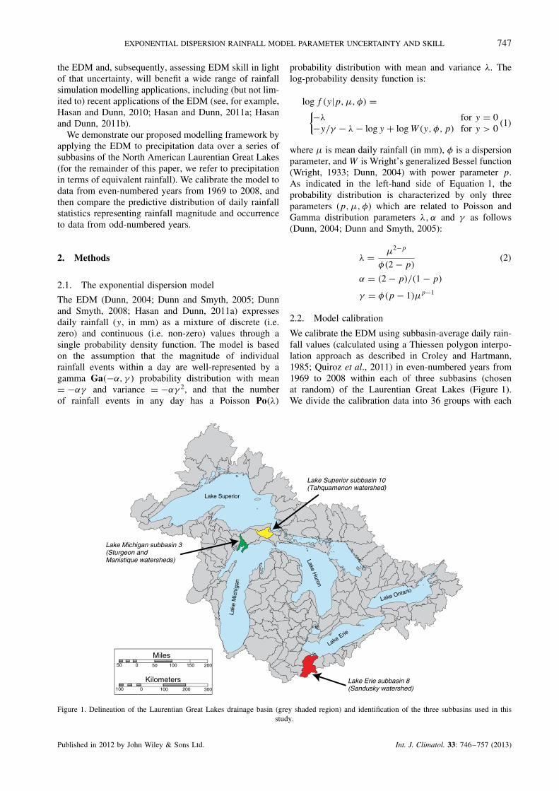
We calibrate the EDM using subbasin-average daily rain-fall values (calculated using a Thiessen polygon interpo-lation approach as described in Croley and Hartmann,1985; Quiroz et al., 2011) in even-numbered years from1969 to 2008 within each of three subbasins (chosenat random) of the Laurentian Great Lakes (Figure 1).We divide the calibration data into 36 groups with each

Lake Superior

Lake

Mic

higa

n

Lake Huron

Lake Erie

Lake Ontario

Lake Michigan subbasin 3(Sturgeon andManistique watersheds)

Lake Superior subbasin 10(Tahquamenon watershed)

Lake Erie subbasin 8(Sandusky watershed)

Miles100 2001505050 0

Kilometers100 200100 3000

Figure 1. Delineation of the Laurentian Great Lakes drainage basin (grey shaded region) and identification of the three subbasins used in thisstudy.

Published in 2012 by John Wiley & Sons Ltd. Int. J. Climatol. 33: 746–757 (2013)

748 A. D. GRONEWOLD et al.

group comprised of data from one of the three sub-basins and from 1 of the 12 months of the year. The firstdata set, for example, includes 620 daily rainfall values,each observed in the month of January during an even-numbered year from 1969 to 2008 in Lake Superior sub-basin 10 (1 subbasin × 20 months × 31 days per month).Rainfall values from odd-numbered years are used formodel confirmation (for further discussion of model con-firmation routines, see Reckhow and Chapra, 1983; Efronand Tibshirani, 1993; Gronewold et al., 2009).

We estimate parameters of the EDM (i.e. p,µ, φ) bydrawing samples from the posterior probability distribu-tion for each using a Bayesian MCMC approach. Webegin by defining the likelihood of the data given a setof model parameters which, for �y ≡ (y1, . . . , yn), whenapplied to the EDM (Equation 1), is L(�y|p,µ, φ) ≡∏n

i f (yi |p,µ, φ). We note that the product form for thelikelihood implicitly assumes that daily rainfall valuesare independent. Previous research (see, for example,Hosseini et al., 2011) suggests that daily rainfall values,however, may be correlated. Our procedure for testingthis assumption is described in Section 2.3.1.

We then define a uniform prior distribution on theEDM parameters, π(p,µ, φ), of the form:

π(p,µ, φ) ∝ 1, (where 1 < p < 2, µ > 0, φ ≥ 0).

(3)

We selected a non-informative prior so that the posteriorparameter distribution would be minimally influencedby our a priori beliefs about the parameter values. Werecognize that our proposed non-informative prior mayprove problematic if little data are available to informthe parameters. However, we found that sufficient dataare available to yield robust parameter inference withany vague prior. More specifically, we found that, in ourstudy, model parameters are identifiable with as few as20 observations, but not with 10. It is possible that studiesin other regions (such as those with drier climes) mightrequire alternative priors or larger data sets (or both) inorder to identify model parameters. For further discussionon selection of prior probability distributions, see Press(2003).

Following Bayes’ theorem, the posterior probabilitydistribution of the EDM parameters is then:

π(p, µ, φ|�y) ∝ L(�y|p,µ, φ) × π(p,µ, φ)

∝n∏i

f (yi |p,µ, φ). (4)

For each iteration in the MCMC chain, we calculatethe joint posterior probability density of the data andcandidate model parameters (i.e. Equation 4) using thedtweedie function in the tweedie package (fordetails, see Dunn and Smyth, 2005; Dunn and Smyth,2008) in the statistical software program R (Ihaka andGentleman, 1996). Details of the MCMC algorithm areincluded in the Appendix.

We ran the MCMC algorithm three times with differentinitial parameter values, leading to three parallel ‘chains’for each parameter. We ran all three chains for 20,000iterations, and removed the first 10,000 as a ‘burn-in’ period (Gelman et al., 2004). We then thinned theremaining 10,000 iterations at a 1 : 10 ratio, leaving a totalof 3,000 simulated samples (1,000 per chain × 3 chains)from the posterior distribution for each parameter. Wetested each MCMC run for convergence by calculatingthe potential scale reduction factor R and verifying thatit was close to 1.0 for all MCMC chains. For details, seeGelman et al. (2004, p. 297).

2.3. Model confirmationOne goal of this paper is to assess the EDM as a potentialtool for documenting historical dynamics, and simulatingfuture dynamics (perhaps based on results of regional-scale climate models). However, doing so presupposesthat the EDMs can accurately hindcast observed aggre-gate rainfall patterns. Therefore, a confirmatory study isnecessary. While we recognize many statistics could beused to evaluate model accuracy (for further discussion,see Stow et al., 2009), we base our model confirmationon an assessment of two metrics which correspond torainfall frequency and magnitude, respectively.

2.3.1. Rainfall frequency

We begin by calculating the predictive distribution ofthe number of days with no measurable rainfall (zi,j )in month i (i ∈ 1, . . ., 12) and subbasin j (j ∈ 1, . . ., 3)by following the common assumption that zi,j has abinomial Bi(zi,j |ni, θi,j ) probability distribution with ni

equal to the total number of days in month i, and θi,j , theposterior probability of no measurable rainfall in monthi and subbasin j . Following Dunn (2004) and equation1, θ is equal to exp(−λ). The predictive distribution forzi,j given a set of observed daily rainfall values �yi,j ineven-numbered years from 1969 to 2008 is then:

p(zi,j |�yi,j , ni) =∫ 1

0

(ni

zi,j

)θ

zi,j

i,j ×

(1 − θi,j )ni−zi,j π(θi,j |�yi,j )dθi,j (5)

where π(θi,j |�yi,j ), the posterior probability distribu-tion of θi,j given �yi,j (based on m MCMC samplesθi,j,1, . . . , θi,j,m) is:

π(θi,j |�yi,j ) = 1

m

m∑k=1

δ(θi,j,k − θi,j ) (6)

and δ(. . .) is the Dirac delta function with unit probabilitymass. The predictive probability distribution of zi,j isthen:

p(zi,j |�yi,j , ni) = 1

m

(ni

zi,j

) m∑k=1

[θ

zi,j

i,j,k(1 − θi,j,k)ni−zi,j

]

(7)

= 1

m

m∑k=1

dbinom(zi,j |ni, θi,j,k) (8)



where dbinom is the binomial probability distributiondensity function in the statistical software program R. Wethen calculate the 95% prediction set for the number ofdays in a month with no measurable precipitation. Here,following Gronewold and Wolpert (2008), we define a95% prediction set as the set of ‘highest probability’integer values between 0 and ni (the number of days inmonth i) for which the cumulative probability mass is atleast 0.95. For illustrative examples of 95% predictionsets, see Figures 3 and 4 in Gronewold and Wolpert(2008) and Figures 5 and 6 in Gronewold et al. (2011b).We then calculate the corresponding 95% predictionintervals for the fraction of days in a month with nomeasurable precipitation by dividing the bounds of the95% set by the respective number of days in each month.

To test our assumption of conditional independence ofdaily rainfall values, we calculate the predictive distri-bution for two quantities; the number of days with nomeasurable rainfall in a given month given that the pre-vious day had no measurable rainfall (which we identifyas z0), and the number of days with no measurable rain-fall in a given month given that the previous day hadmeasurable rainfall (which we refer to as z′). These twopredictive distributions can be expressed (following thelogic of Equations 5 through 8) as (for simplicity, wehave removed i and j from Equations 9 and 10):

p(z0|�y, n0) = 1

m

m∑k=1

dbinom(z0|n0, θk) (9)

and,

p(z′|�y, n′) = 1

m

m∑k=1

dbinom(z′|n′, θk) (10)

where n0 is the total number of days in a given monthpreceded by a day with no rainfall, and n′ is the totalnumber of days in a given month preceded by a day withrainfall. Following the procedure described above, wethen calculate the 95% prediction set for both z0 and z′,and compare both to observed values from the calibrationand confirmation periods.

2.3.2. Rainfall magnitude

To assess the EDM’s potential for simulating daily rain-fall magnitude, we calculate the probability distributionof measurable daily rainfall (i.e. daily rainfall amountsgreater than zero) for each subbasin-month combinationand compare it to the observed probability distributionof measurable daily rainfall. We do this by entering all3000 MCMC samples from each EDM parameter pos-terior distribution into the rtweedie function in thetweedie package (Dunn and Smyth, 2005; Dunn andSmyth, 2008), an approach that generates (for one iter-ation of the rtweedie function) 3,000 samples fromthe posterior predictive distribution of y. We note herethat this approach is analogous to simulating a 3,000-daylong time series of daily rainfall values.

To fully capture intrinsic variability in the probabilitydistribution of daily rainfall values (due, in part, to afinite number of samples from the EDM parameter jointposterior distribution), we repeat this procedure 10,000times, excluding from the final set of simulated dailyrainfall values those which equal zero (a schematic, anda slightly more detailed description of this procedure, areincluded in Figure 8 and the Appendix, respectively). Wethen calculate the quantiles of the observed measurablerainfall times series (separately for both calibration andconfirmation periods) and the quantiles from each ofthe 10,000 sets of simulated rainfall values. Finally,we compare each observed rainfall value to the setof simulated rainfall values from the correspondingquantile of the simulated sets. Our approach differs fromconventional quantile–quantile comparisons because itexplicitly depicts uncertainty and (unlike comparisonsof quantile residuals) identifies where potential sourcesof bias are likely to arise from the simulated timeseries.

3. Results

3.1. Model calibration

Our model calibration results indicate several patternsin the EDM parameters both within and across each ofthe subbasins (Figure 2). For example, the 95% highestposterior density (HPD) regions (Figure 2) suggest thatthe EDM power parameter, p, varies throughout theyear when fit to the Lake Superior and Lake Michigansubbasin data, but that it is relatively consistent andsomewhat higher throughout the year when fit to theLake Erie subbasin data. The relatively high values andlow variability of the power parameter for the LakeErie watershed likely reflect a combination of empiricalevidence (Figure 4) indicating that the fraction of dayswith no rainfall in the Lake Erie watershed is relativelyconsistent throughout the year, and that the mean dailyrainfall is also relatively high and relatively consistentfor the Lake Erie watershed as well. For a more rigorousassessment of EDM power parameter dynamics, seeDunn (2004) and Hasan and Dunn (2011a).

We also find that the expected value of daily rain-fall µ follows a seasonal pattern with peak values forLake Superior subbasin 10 in April, for Lake Michigansubbasin 3 in September, and for Lake Erie subbasin8 in June. We could assess mean daily rainfall values(i.e. calculate a value for µ) through an empirical dataassessment as well, however assessing the posterior dis-tribution of µ in a Bayesian framework explicitly prop-agates data variability through the posterior distributioninto uncertainty in rainfall forecasts. Finally, we find thatthe dispersion parameter, φ, varies from season to sea-son, although the pattern differs among subbasins (bottomrow, Figure 2).

Our parameter correlation assessment indicates thatthe expected value of daily rainfall µ is independent of



1.55

1.65

1.75

p

Lake Superior (10)

J F M J J A S O D

23

45

67

φ

Month

J F M J J A S O D

Month

Lake Michigan (3) Lake Erie (8)

12

34

µ

J F M J J A S O D

Month

NMA N

NMA

MA

Figure 2. Model calibration results, including posterior distribution 95% highest posterior density (HPD) regions (vertical lines) for eachcombination of EDM parameter (rows) and subbasin (columns). Calibration results are based on conditioning the EDM to rainfall data in

even-numbered years from 1969 to 2008.

both the dispersion parameter φ and power parameter p,based on the orientation of the marginal posterior densitycontours in the {µ, p}- and {µ, φ}-planes (middle leftand bottom centre panels in Figure 3, respectively). Wefind, however, that φ and p are positively correlated(middle panel Figure 3). The patterns in Figure 3 arebased on calibrating the EDM to January rainfall data inLake Superior subbasin 10, however we find (results notshown) they represent parameter relationships when theEDM is calibrated using rainfall data from other monthsand other subbasins.

3.2. Model confirmation

3.2.1. Rainfall frequency

A comparison between the observed fraction of daysin a given month with no measurable rainfall and thepredictive distribution indicates that the EDM slightlyunderestimates the probability of zero rainfall (Figure 4).The 95% prediction regions contain approximately 84%of the observations from the calibration period and 82%from the confirmation period across all subbasin–monthcombinations. This proportion does not vary systemat-ically within subbasins across months, nor is there asystematic tendency to miss either high or low extremevalues. We recognize that this incomplete coverage couldoccur for several reasons, including temporal depen-dence in the EDM, as well as the use of Thiessen-weighting to synthesize gauge-based observations. Futurework will focus on differentiating these and otherpossibilities.

Our results also suggest that the EDM does not fullyrepresent the temporal dependence of daily rainfall val-ues. For example, we found that the 95% predictioninterval for z0 (using EDM parameter values condi-tioned under an assumption of conditional independence)included 71% of observations from the calibration period,and 69% of observations from the confirmation period.Similarly, we found that the 95% prediction interval for z′included 72% and 74% of the observations from the cal-ibration and confirmation periods, respectively. The rel-atively lower skill of the EDM when forecasting rainfallvalues conditioned on their antecedent conditions impliesthat p(z|�y, n) �= p(z0|�y, n0) �= p(z′|�y, n′), and suggeststhat the EDM in its current form is more suitable for mod-elling monthly precipitation values (assuming less tempo-ral dependence when aggregating from daily to monthlyscales) or that it may need to be modified if appliedto daily rainfall values. We find that previous applica-tions of the EDM (Dunn, 2004; Dunn and Smyth, 2005;Hasan and Dunn, 2011a), which progressively gravitatetowards a focus on monthly rainfall data, do not explic-itly acknowledge (through, for example, the type of skillassessment we present here) nor emphasize (perhaps inqualitative terms) this important distinction. One possi-bility to incorporate the dependence structure would be touse the Tweedie distribution in a generalized linear mod-elling framework (Hasan and Dunn, 2011a), incorporat-ing covariates such as lags in the observed daily rainfall.

3.2.2. Rainfall magnitude

Generally, the EDM provides a reasonable reproductionof the probability distribution of measurable daily rainfallfor each subbasin–month combination, indicated by the



2.0 2.5 3.0 3.5

Den

sity

µ φ

p

µ

1.64

1.68

1.72

p

Density

5.0 5.5 6.0 6.5 7.0

2.0

2.5

3.0

3.5

µ

φ

Figure 3. Histograms and contour plots of the marginal and joint posterior probability distributions (respectively) for EDM parameters. Resultsshown are based on calibrating the EDM to daily rainfall values from January across even-numbered years from 1969 through 2008 in Lake

Superior subbasin 10 (Figure 1). The scale of the probability density axis (labeled ‘Density’) is intentionally removed from each histogram.

Lake

Sup

erio

r (1

0)

0.0

0.4

0.8

Jan Feb Mar Apr May Jun Jul Aug Sep Oct Nov Dec

Lake

Mic

higa

n (3

)

Fra

ctio

n of

day

s w

ith n

o m

easu

rabl

e ra

infa

ll

0.0

0.4

0.8

Lake

Erie

(8)

0.0

0.4

0.8

Figure 4. Model confirmation results, including 95% prediction intervals (grey regions) for the fraction of days with no measurable rainfall ineach month. In each panel, dots represent the observed fraction of days with no measurable rainfall in a given month from 1969 (left-mostdot in each panel) through 2008 (right-most dot in each panel). Blue dots represent the fraction of days with no measurable rainfall in a givenmonth in even years (calibration data), and red dots represent the fraction of days with no measurable rainfall in a given month in odd years

(confirmation data).



Figure 5. Comparison between observed and simulated rainfall values over Lake Superior subbasin 10 from the same quantile. Vertical linesindicate the range of simulated values from a particular quantile generated using all MCMC samples from the EDM joint parameter posteriordistribution. Blue lines represent calibration data, and red lines represent confirmation data. The 1 : 1 line (black) is shown for reference. Axes

are presented at square-root scale to improve clarity.

fact that most of the vertical blue (calibration period)and red (confirmation period) lines in Figures 5 through7 intersect the 1 : 1 line. Each vertical line indicates therange of simulated daily rainfall values for each quantilefrom the corresponding set of observed non-zero dailyrainfall values. Put differently, the location of each verti-cal line along the x-axis in each panel corresponds to anobserved daily rainfall value. The corresponding height ofeach vertical line reflects the uncertainty in the predicteddaily rainfall value from the quantile of the observeddaily rainfall value. Within a particular panel in Figures 5through 7, relatively short vertical lines that intersect the

1 : 1 line indicate a predictive distribution for daily rain-fall (for the subbasin–month combination represented bythat panel) which is similar to the observed rainfall prob-ability distribution. Wide vertical lines in any given panelthat intersect the 1 : 1 line indicate that there is signifi-cant uncertainty in a particular quantile of the predictivedistribution, but that the observed rainfall value from thesame quantile is within the predicted range of values.

While the EDM appears to reproduce the general fea-tures of the probability distribution of daily rainfall, weobserve, as expected, significant variability in the EDM-derived upper quantiles of the daily rainfall distribution.



Figure 6. Comparison between observed and simulated rainfall values over Lake Michigan subbasin 3 from the same quantile. Vertical linesindicate the range of simulated values from a particular quantile generated using all MCMC samples from the EDM joint parameter posteriordistribution. Blue lines represent calibration data, and red lines represent confirmation data. The 1 : 1 line (black) is shown for reference. Axes

are presented at square-root scale to improve clarity.

For example, the upper left-hand panel of Figure 5 indi-cates that our calibrated model (for January in Lake Supe-rior subbasin 10) simulates extreme daily rainfall rangingbetween roughly 28 and 135 mm (as indicated by theextent of the right-most red and blue vertical lines) whilethe corresponding rainfall values from the same quantilein the observed data sets were about 73 mm (calibrationyears) and 41 mm (validation years).

4. Discussion and conclusions

This paper assesses the EDM in a Bayesian MCMCframework for simulating daily rainfall in three sub-basins of the North American Laurentian Great Lakes.

We have shown that, within this framework, explic-itly acknowledging variability in daily rainfall timeseries data through uncertainty and correlation in theEDM parameter joint posterior probability distribution(Figure 3) leads to appropriate representation of uncer-tainty in simulated daily rainfall magnitude and occur-rence. By ‘appropriate representation of uncertainty’ wemean that the uncertainty expressed in EDM forecastsneither greatly exceeds, nor significantly underestimatesthe variability observed in independent rainfall timeseries. We base this assessment on two measures of modelskill; (1) the fraction of 95% prediction intervals whichinclude the observed fraction of days with no measurablerainfall in an independent confirmation data set, and (2)a quantile-based comparison of simulated and observed



Figure 7. Comparison between observed and simulated rainfall values over Lake Erie subbasin 8 from the same quantile. Vertical lines indicatethe range of simulated values from a particular quantile generated using all MCMC samples from the EDM joint parameter posterior distribution.Blue lines represent calibration data, and red lines represent confirmation data. The 1 : 1 line (black) is shown for reference. Axes are presented

at square-root scale to improve clarity.

daily rainfall time series. Other metrics and assessmenttechniques could be used, including total monthly orannual rainfall amounts, coupled, perhaps, with an anal-ysis of the histograms of Bayesian posterior predictivep-values for these metrics. For a detailed description ofthese and similar assessment metrics, including probabil-ity integral transform and verification rank histograms,see Raftery et al. (2005); Elmore (2005); Gronewoldet al. (2009). We plan to explore these alternatives infuture applications of the EDM (including, for example,those which support probabilistic approaches to resource

management, as described in Gronewold and Borsuk,2009).

In addition to providing a robust basis for quantify-ing uncertainty in EDM parameters and forecasts, ourBayesian MCMC calibration approach provides a con-venient alternative to conventional model calibration andforecasting schemes. For example, stochastic rainfall sim-ulation models are often calibrated through optimizationalgorithms that yield parameter point estimates and pro-duce deterministic comparisons between simulated andobserved time series metrics (which, in some cases,



include procedures for ‘matching’ observed and simu-lated statistics using parameter perturbations, as describedin Burton et al., 2008). Our approach provides an alter-native that explicitly acknowledges uncertainty and vari-ability in rainfall dynamics. In doing so, our applicationof the EDM allows us to choose between either reflectingthe same degree of variability observed in historic timeseries in future simulations, or modifying the location andscale of EDM parameters (based, perhaps, on regional cli-mate model outputs). The latter approach acknowledgesand meets the growing need for models which reflectchanging conditions over time (Milly et al., 2008) andprovides an alternative to scenario-weighting approaches(for similar applications and further discussion, see (Lof-gren et al., 2002). Furthermore, we recognize that whilewe have not rigorously tested our assumption of decadalstationarity in this particular application of the EDM,the rainfall data from 1969 through 2008 in the threesubbasins studied does not appear to demonstrate a sig-nificant trend over this 40 year period (Figure 4), withthe exception of the frequency of daily rainfall events inSeptember in the Lake Superior Tahquamenon watershed(subbasin 10), which appears to be decreasing (i.e. thefraction of days with no measurable rainfall is increas-ing). Regardless, our application of the EDM can easilybe transferred to a more comprehensive regional or hier-archical analysis of precipitation patterns within the GreatLakes basin, and we view this as an area for futureresearch. A regional frequency analysis, in particular,could potentially reduce some of the variability in ourestimates (Figures 5–7) of extreme rainfall quantiles (forfurther discussion, see Trefry et al., 2005; Ribatet et al.,2007).

Our study also underscores pending difficulties associ-ated with downscaling regional climate change scenariosinto local scale dynamics, particularly in regions (suchas the Laurentian Great Lakes) with significant local-scale spatial climate variability. For example, the LakeSuperior Tahquamenon watershed (subbasin 10) and theLake Michigan Sturgeon and Manistique watershed (sub-basin 3) are within 50 miles (roughly 80 kilometers) ofeach other (Figure 1), yet the rainfall dynamics in eachdiffer (Figure 4), due in part to different weather andwind patterns over and adjacent to Lake Superior. Bycalibrating the EDM to local scale climate data, ourapproach serves as an ideal cornerstone for a futurecoupled RCM-EDM which propagates regional climatepatterns into local-scale rainfall (and other weather com-ponent) dynamics.

In this process, we have identified three areas forimprovement. First, we recognize that EDM performancecould be improved through an analysis of potentialthresholds for ‘measurable’ rainfall amounts (Burtonet al., 2008) and corrections for potential bias thesethresholds might introduce. Second, we acknowledgethat temporal dependencies in daily rainfall data are notroutinely captured by the EDM, and therefore the EDM islikely most suitable for application to monthly time seriesdata. We underscore here how our assessment provides a

robust quantitative basis for making this distinction, andthat future research might focus on supplementing theEDM with algorithms for expressing autocorrelation ona daily time scale. Third, the daily rainfall values we usedhere are, in fact, averaged (based on multiple individualrain gauges) over each subbasin, an approach whichcould overestimate the frequency and underestimate theintensity of daily rainfall dynamics (Bates et al., 1998).We intend, in future research, to calibrate the EDMto individual rain gauge data and then combine theEDM parameters using a Bayesian model averaging orhierarchical approach (Raftery et al., 2005; Gelman andHill, 2007; Ancelet et al., 2010).

Acknowledgements

The authors thank Brent Lofgren, Anne Clites, and twoanonymous reviewers whose comments improved theclarity and overall quality of this paper. The authors alsothank Cathy Darnell for providing editorial and graphicssupport. This paper is GLERL contribution number 1624.

A1. Appendix

A1.1. Markov chain Monte Carlo (MCMC)algorithm

The algorithm used in this paper is a three-parameterMetropolis-Hastings algorithm, which is a type ofMarkov chain Monte Carlo (MCMC) algorithm usedto generate random samples from intractable probabilitydensities. The algorithm is implemented iteratively withk being the current iteration, and the parameter set (or‘state’) for a particular iteration is defined as {pk, µk, φk}.A trial state {p′, µ′, φ′} is generated using a trivariatenormal distribution centred at the current state:

(p′, µ′, φ′) ∼ N3 ({pk, µk, φk}, �)

where � is a covariance matrix.The likelihood and prior distribution are evaluated at

this trial state. Alternatively, one can change a randomsubset of the parameters at each iteration rather than thewhole set. The trial state is accepted with probability

Pr{p′, µ′, φ′ → pk+1, µk+1, φk+1}= min

(1,

L(�y|p′, µ′, φ′) × π(p′, µ′, φ′)L(�y|pk, µk, φk) × π(pk, µk, φk)

)

and if the trial state is not accepted, the current state{pk, µk, φk} is retained at iteration k + 1.

The set of states over all iterations constitutes a‘chain’. The acceptance–rejection step ensures that thechain will eventually converge to the posterior distri-bution, π(p,µ, φ|�y). Convergence was checked usingthe CODA package in R, and we found no evidence ofnon-convergence.



Figure 8. Schematic representation of procedure for simulating the probability distribution of measurable daily rainfall amounts (see AppendixA2 for details).

Generally, one wants the Metropolis-Hastings algo-rithm to accept between 20% and 50% of the trial states.Too many or too few mean the chain is not samplingthe posterior efficiently. This fraction can be tuned bytrying different values of �. After some experimenta-tion, we found that a diagonal covariance with � =diag(0.002, 0.07, 0.07) yields a 32% acceptance fraction.

A2. Simulating the probability distribution ofmeasurable daily rainfall

Figure 8 provides a schematic representation of our pro-cedure for simulating the probability distribution of themagnitude of measurable daily rainfall events. After sim-ulating 3000 MCMC samples from the posterior proba-bility distribution for each EDM parameter (µ, p, φ) fora given set of observed daily rainfall values −→y for aparticular month and subbasin (as described in the pre-vious appendix and in Section 2.2, and represented bythe upper-half of Figure 8), we systematically pass eachtriplet of parameter values from the MCMC chain tothe rtweedie package (Dunn and Smyth, 2005, 2008).We then use the rtweedie package to simulate 10,000daily rainfall values from an EDM for each triplet. Forexample, in Figure 8, a blue vertical line passes throughthe first value of µ, p, and φ in each MCMC chain(represented as µ1, p1, and φ1) which are passed to thertweedie package to simulate 10,000 rainfall valuesfor that particular triplet. The 10,000 simulated rainfallamounts using µ1, p1, and φ1 are represented by thevector y1,1, y1,2, . . . , y1,10 000 (highlighted in blue) in thearray in the bottom-right of Figure 8. We repeat this pro-cedure for the second triplet of parameter values (high-lighted in red in Figure 8) and continue up to the final(i.e. 3,000th) value in each MCMC chain (highlighted in

green in Figure 8). The set of simulated, non-zero valuesfrom the resulting array (bottom-right corner of Figure 8)constitutes our approximated probability distribution ofmeasurable daily rainfall values for the given month andsubbasin.

References

Ancelet S, Etienne M, Benoıt H, Parent E. 2010. Modelling spatial zero-inflated continuous data with an exponentially compound Poissonprocess. Environmental and Ecological Statistics 17(3): 347–376.

Bates B, Charles S, Hughes J. 1998. Stochastic downscaling ofnumerical climate model simulations. Environmental Modelling &Software 13(3–4): 325–331.

Berry DA. 1996. Statistics: A Bayesian Perspective, Duxbury Press:Belmont, CA.

Beven K. 2001. How far can we go in distributed hydrologicalmodelling? Hydrology and Earth System Sciences 5(1): 1–12.

Bolstad WM. 2004. Introduction to Bayesian Statistics, Wiley-Interscience: Hoboken, NJ.

Burton A, Kilsby C, Fowler H, Cowpertwait P, O’Connell P. 2008.RainSim: a spatial-temporal stochastic rainfall modelling system.Environmental Modelling & Software 23(12): 1356–1369.

Cannon A. 2008. Probabilistic multisite precipitation downscalingby an expanded Bernoulli-Gamma density network. Journal ofHydrometeorology 9(6): 1284–1300.

Chapman T. 1998. Stochastic modelling of daily rainfall: the impactof adjoining wet days on the distribution of rainfall amounts.Environmental Modelling & Software 13(3–4): 317–324.

Cowpertwait P. 1994. A generalized point process model for rainfall.Proceedings: Mathematical and Physical Sciences 447(1929):23–37.

Cowpertwait P. 1995. A generalized spatial-temporal model of rainfallbased on a clustered point process. Proceedings: Mathematical andPhysical Sciences 450(1938): 163–175.

Croley TE, Hartmann HC. 1985. Resolving Thiessen polygons. Journalof Hydrology 76(3–4): 363–379.

Dunn PK. 2004. Occurrence and quantity of precipitation can bemodelled simultaneously. International Journal of Climatology 24:1231–1239.

Dunn PK, Smyth GK. 2005. Series evaluation of Tweedie exponentialdispersion model densities. Statistics and Computing 15(4):267–280.



Dunn PK, Smyth GK. 2008. Evaluation of Tweedie exponentialdispersion model densities by Fourier inversion. Statistics andComputing 18(1): 73–86.

Efron B, Tibshirani RJ. 1993. An Introduction to the Bootstrap,Chapman & Hall/CRC: New York.

Elmore K. 2005. Alternatives to the chi-square test for evaluating rankhistograms from ensemble forecasts. Weather and Forecasting 20:789–795.

Ferguson C, Husman AMD, Altavilla N, Deere D, Ashbolt N. 2003.Fate and transport of surface water pathogens in watersheds. CriticalReviews in Environmental Science and Technology 33(3): 299–361.

Fernandes M, Schmidt A, Migon H. 2009. Modelling zero-inflatedspatio-temporal processes. Statistical Modelling 9(1): 3.

Fowler H, Blenkinsop S, Tebaldi C. 2007. Linking climate changemodelling to impacts studies: recent advances in downscalingtechniques for hydrological modelling. International Journal ofClimatology 27(12): 1547–1578.

Friederichs P, Hense A. 2007. Statistical downscaling of extremeprecipitation events using censored quantile regression. MonthlyWeather Review 135(8): 2365–2378.

Furrer E, Katz R. 2007. Generalized linear modeling approach tostochastic weather generators. Climate Research 34(2): 129.

Gabriel K, Neumann J. 1962. A Markov chain model for dailyrainfall occurrence at Tel Aviv. Quarterly Journal of the RoyalMeteorological Society 88(375): 90–95.

Gelman A, Carlin JB, Stern HS, Rubin DB. 2004. Bayesian DataAnalysis, Chapman & Hall/CRC: Boca Raton, FL.

Gelman A, Hill J. 2007. Data Analysis Using Regression andMultilevel/Hierarchical Models, Cambridge University Press: NewYork, NY.

Grant SB, Sanders BF, Boehm AB, Redman JA, Kim JH, MrseRD, Chu AK, Gouldin M, McGee CD, Gardiner NA, Jones BH,Svejkovsky J, Leipzig GV. 2001. Generation of Enterococci bacteriain a coastal saltwater marsh and its impact on surf zone water quality.Environmental Science & Technology 35(12): 2407–2416.

Green J. 1964. A model for rainfall occurrence. Journal of the RoyalStatistical Society. Series B (Methodological) 26(2): 345–353.

Gronewold AD, Borsuk M. 2009. A software tool for translatingdeterministic model results into probabilistic assessments of waterquality standard compliance. Environmental Modelling & Software24(10): 1257–1262.

Gronewold AD, Clites A, Hunter T, Stow C. 2011a. An appraisal ofthe Great Lakes advanced hydrologic prediction system. Journal ofGreat Lakes Research 37: 577–583.

Gronewold AD, Myers L, Swall JL, Noble RT. 2011b. Addressinguncertainty in fecal indicator bacteria dark inactivation rates. WaterResearch 45: 652–664.

Gronewold AD, Qian SS, Wolpert RL, Reckhow KH. 2009. Calibratingand validating bacterial water quality models: a Bayesian approach.Water Research 42: 2688–2698.

Gronewold AD, Wolpert RL. 2008. Modeling the relationship betweenmost probable number (MPN) and colony-forming unit (CFU)estimates of fecal coliform concentration. Water Research 42(13):3327–3334.

Hasan M, Dunn P. 2010. A simple Poisson-gamma model for modellingrainfall occurrence and amount simultaneously. Agricultural andForest Meteorology 150(10): 1319–1330.

Hasan M, Dunn P. 2011a. Two Tweedie distributions that are near-optimal for modelling monthly rainfall in Australia. InternationalJournal of Climatology 31(9): 1389–1397.

Hasan M, Dunn P. 2011b. Understanding the effect of climatologyon monthly rainfall amounts in Australia using Tweedie GLMs.International Journal of Climatology. DOI: 10.1002/joc.2332.

Haylock M, Cawley G, Harpham C, Wilby R, Goodess C. 2006.

Downscaling heavy precipitation over the United Kingdom: acomparison of dynamical and statistical methods and their futurescenarios. International Journal of Climatology 26(10): 1397–1415.

Holman K, Gronewold AD, Notaro M, Zarrin A. 2012. Improvinghistorical precipitation estimates over the Lake Superior basin.Geophysical Research Letters 39(3): L03405.

Hosseini R, Le N, Zidek J. 2011. Selecting a binary Markov modelfor a precipitation process. Environmental and Ecological Statistics.18(4): 795–820, DOI: 1–2610.1007/s10651-010-0169-1.

Ihaka R, Gentleman R. 1996. R: a language for data analysis andgraphics. Journal of Computational and Graphical Statistics 5(3):299–314.

Lofgren BM, Quinn FH, Clites AH, Assel RA, Eberhardt AJ,Luukkonen CL. 2002. Evaluation of potential impacts on GreatLakes water resources based on climate scenarios of two GCMs.Journal of Great Lakes Research 28(4): 537–554.

Milly PC, Betancourt J, Falkenmark M, Hirsch RM, Kundzewicz ZW,Lettenmaier DP, Stouffer RJ. 2008. Stationarity is dead: whitherwater management? Science 319(5863): 573–574.

Onof C, Wheater H. 1993. Modelling of British rainfall using arandom parameter Bartlett-Lewis rectangular pulse model. Journalof Hydrology 149(1–4): 67–95.

Onof C, Wheater H. 1994. Improvements to the modelling ofBritish rainfall using a modified random parameter Bartlett-Lewisrectangular pulse model. Journal of Hydrology 157(1–4): 177–195.

Press SJ. 2003. Subjective and Objective Bayesian Statistics: Principles,Models, and Applications, Wiley-Interscience: Hoboken, NJ.

Quiroz R, Yarlequ C, Posadas A, Mares V, Immerzeel WW. 2011.Improving daily rainfall estimation from ndvi using a wavelettransform. Environmental Modelling & Software 26(2): 201–209.

Raftery A, Gneiting T, Balabdaoui F, Polakowski M. 2005. UsingBayesian model averaging to calibrate forecast ensembles. MonthlyWeather Review 133(5): 1155–1174.

Reckhow KH. 1999. Water quality prediction and probability networkmodels. Canadian Journal of Fisheries and Aquatic Sciences 56(7):1150–1158.

Reckhow KH, Chapra SC. 1983. Confirmation of water quality models.Ecological Modelling 20(2–3): 113–133.

Ribatet M, Sauquet E, Gresillon J, Ouarda T. 2007. A regional BayesianPOT model for flood frequency analysis. Stochastic EnvironmentalResearch and Risk Assessment 21(4): 327–339.

Stern R, Coe R. 1984. A model fitting analysis of daily rainfall data.Journal of the Royal Statistical Society. Series A (General) 147(1):1–34.

Stow CA, Jolliff J, Jr. Doney DJM, Allen SC, Friedrichs JI,Rose MA, Wallhead KA. P 2009. Skill assessment for coupledbiological/physical models of marine systems. Journal of MarineSystems 76(1–2): 4–15.

Timbal B, Fernandez E, Li Z. 2009. Generalization of a statisticaldownscaling model to provide local climate change projectionsfor Australia. Environmental Modelling & Software 24(3):341–358.

Trefry C, Watkins D, Jr. Johnson D. 2005. Regional rainfallfrequency analysis for the State of Michigan. Journal of HydrologicEngineering 10: 437.

Velghe T, Troch P, De Troch F, Van de Velde J. 1994. Evaluation ofcluster-based rectangular pulses point process models for rainfall.Water Resources Research 30(10): 2847–2858.

Wagener T, Wheater HS. 2006. Parameter estimation and regional-ization for continuous rainfall-runoff models including uncertainty.Journal of Hydrology 320(1–2): 132–154.

Wright E. 1933. On the coefficients of power series having essentialsingularities. Journal of the London Mathematical Society 8: 71–79.


quantifying parameter uncertainty and assessing the … that uncertainty, will beneﬁt a wide range...

Documents