Quaderni di Conservazione della Natura

Ettore Randi, Cristiano Tabarroni and Silvia Rimondi

Gene

tics

CIT

ES

ISSN 1592-2901

MINISTERO DELL’AMBIENTEE DELLA TUTELA DEL TERRITORIO

Direzione Protezione della Natura

ISTITUTO NAZIONALEPER LA FAUNA SELVATICA

“ALESSANDRO GHIGI”

This publication series, specifi cally focused on conservation problems of Italian wildlife, is the result of a co-operation between the Nature Protection Service of the Italian Ministry of Environment and the National Institute for Wildlife Biology “A. Ghigi”. Aim of the series is to promote a wide circulation of the strategies for the wildlife preservation and management worked up by the Ministry of Environment with the scientifi c and technical support of the National Institute for Wildlife Biology.

The issues covered by this series range from general aspects, based on a multidisciplinary and holistic approach, to management and conservation problems at specifi c level.

La collana “Quaderni di Conservazione della Natura” nasce dalla collaborazione instaurata tra il Ministero dell’Ambiente, Servizio Protezione della Natura e l’Istituto Nazionale per la Fauna Selvatica “A. Ghigi”. Scopo della collana è quello di divulgare le strategie di tutela e gestione del patrimonio faunistico nazionale elaborate dal Ministero con il contributo scientifi co e tecnico dell’I.N.F.S.

I temi trattati spaziano da quelli di carat-tere generale, che seguono un approccio mul-tidisciplinare ed il più possibile olistico, a quelli dedicati a problemi specifi ci di gestione o alla conservazione di singole specie.

Cover: graphic elaboration by Cristiano TabarroniTranslation in English: Maria Lombardi

EDITORIAL BOARD

ALDO COSENTINO, ALESSANDRO LA POSTA, MARIO SPAGNESI, SILVANO TOSO

MINISTERO DELL’AMBIENTE ISTITUTO NAZIONALE PER LA

E DELLA TUTELA DEL TERRITORIO FAUNA SELVATICA “A. GHIGI” DIREZIONE PROTEZIONE DELLA NATURA

Ettore Randi, Cristiano Tabarroni and Silvia Rimondi

Forensic genetics and the

Washington Convention - CITES

QUADERNI DI CONSERVAZIONE DELLA NATURANUMBER 12/BIS

How to cite this volume:

Randi E., C. Tabarroni and S. Rimondi, 2002 - Forensic genetics and the Washington Convention - CITES. Quad. Cons. Natura, 12 bis, Min. Ambiente - Ist. Naz. Fauna Selvatica.

All rights reserved. No part of this publication may be reproduced, stored in retrieval sistem, or trasmitted in any form (electronic, electric, chemical, mechanical, optical, photostatic) or by any means without the prior permission of Ministero dell’Ambiente e della Tutela del Territorio.

To prohibit selling: this publication is distributed free of charge by Ministero dell’Ambiente e della Tutela del Territorio and Istituto Nazionale per la Fauna Selvatica “A. Ghigi”.

INDEX

INTRODUCTION ......................................................................................... Pag. 5

CONVENTION ON INTERNATIONAL TRADE IN ENDANGERED

SPECIES OF WILD FAUNA AD FLORA - CITES ........................................... " 6

DNA STRUCTURE AND FUNCTION ............................................................ " 15Forensic genetics and DNA fingerprinting ................................ " 15Introduction to DNA fingerprinting ......................................... " 17DNA structure and functions ....................................................... " 19Genetic mutations and polymorphisms .................................... " 34

GENETIC VARIABILITY IN INDIVIDUALS AND POPULATIONS .......................... " 39The process of heredity: Mendel’s laws ..................................... " 39The processes of heredity: association between genes(linkage) ............................................................................................ " 42Genes in populations ..................................................................... " 45Inbreeding ......................................................................................... " 48

MOLECULAR GENETICS: METHODS OF ANALYSING DNA VARIABILITY .......... " 54Collection of biological samples ................................................. " 54Methods to collect biological traces ........................................... " 58Preservation of samples ................................................................. " 59DNA extraction ................................................................................ " 61DNA extraction control .................................................................. " 67Restriction enzymes and restriction fragment length polymorphism analysis (RFLP) ................................................. " 68Analysis of DNA fragments with agarose gel electrophoresis.. " 70Southern blotting ............................................................................ " 73Molecular hybridisation ................................................................ " 75INFS protocol for DNA fingerprinting analysis ........................ " 76Structure of multi-locus probes used in forensic genetics .... " 80Interpretation of DNA fingerprinting ......................................... " 81DNA amplification .......................................................................... " 83Random Amplified Polymorphic DNA (RAPD) ...................... " 86Amplified Fragment Length Polymorphism (AFLP) .............. " 87DNA sequencing ............................................................................... " 88Mitochondrial DNA structure and sequencing ........................ " 93Amplification and analysis of microsatellites ........................... 94

Analysis of microsatellites in automated sequencers .............. Pag. 95Sex chromosomes and gender identification ........................... " 98Similarity determination between DNA fragments, alleles, genotypes and individuals .......................................................... " 101Identification of DNA fragments in DNA fingerprinting analysis with MLP .......................................................................... " 102Estimating allele frequency by binning in multi-locus systems ............................................................................. " 103Identification of alleles in DNA fingerprinting using VNTR systems ............................................................................... " 105Identification of alleles in DNA fingerprinting analysis with microsatellites ............................................................................... " 106

STATISTICAL ANALYSIS OF DATA .................................................................. " 106Frequency distributions ................................................................. " 106Estimation of confidence intervals ............................................. " 110Hypothesis testing .......................................................................... " 111Estimating allelic and genotype frequencies ........................... " 112Estimates of the allele frequencies at codominant loci ............. " 113Estimates of allele frequencies in minisatellites analysed with MLP systems ........................................................................ " 115Estimates of genotype frequencies at multi-locus systems ... " 116

PROBABILITY ............................................................................................. " 117The frequency theory of probability ............................................ 118The subjective theory of probability (Bayesian statistics) ..... " 118The laws of probability ................................................................. " 119Bayes’ Theorem .............................................................................. " 121

APPLICATIONS OF BAYESIAN STATISTICS TO FORENSIC GENETICS ................ " 123Identification .................................................................................... " 123Probability of exclusion ................................................................. " 127Match probability ........................................................................... " 129The probability of identity (PID) ................................................ " 132Paternity testing .............................................................................. " 133

CASE STUDY .............................................................................................. 137Parental testing performed by DNA fingerprinting ................. " 137Parental testing performed by microsatellites .......................... " 140Subspecies identification by mtDNA analysis ............................. " 140

EXECUTIVE SUMMARY ................................................................................ " 143

REFERENCES .............................................................................................. " 145

5

INTRODUCTION

Forensic genetics is going through a period of rapid progress thanks to the development of DNA molecular testing methodologies that have reached levels of precision, repeatability and reliability that were unthinkable until recently. The concept of DNA fingerprinting, that is, genetic fingerprints, has rapidly become part of everyday speech. Molecular methodologies have an elevated capacity of individualisation (every individual, except for identical twins, has a unique genetic arrangement, that differs from any other individual). The results of laboratory tests can be interpreted in the context of population genetics and evaluated using the theory of probability. In this manner the results of laboratory tests can be expressed in a quantitative manner (probabilistically) and evaluated through statistical analysis. The meaning and importance of DNA fingerprinting has long been debated in international scientific literature. The technical aspects concerning the reliability of laboratory testing methodologies, problems regarding sampling as well as theoretical aspects and the application of statistics and genetics in forensic science have been examined in depth. In conclusion forensic genetics today is based on solid theoretical and methodological foundations. The principal aim of forensic genetic testing is to verify the hypothesis that a specific DNA fingerprinting is univocally associated to a particular individual, or that the DNA fingerprinting of an offspring is derived from the DNA fingerprinting of the two putative parents.

The Convention of Washington (CITES) is an international agreement between governments to regulate the trade of plants and animals. The destruction of natural habitats and the uncontrolled trade of wild animals and plants is one of the main causes for the rarefaction and risk of extinction of populations and species. CITES assumes that the control over the sustainable trade of animals, plants and parts and derivatives thereof, is a means of preserving wild populations, above all if the principles of the sustainable use of living species form the basis of national and international legislation. CITES, in fact, requires that the dynamics of threatened species and populations subject to trade, be constantly controlled. Profits to local populations from the sustainable use of natural resources can be partly used in conservation programmes. CITES operates by authorising the issue of import and export permits of those living specimens and their parts and derivatives thereof, that are among the protected species listed in Appendices I and II. The species

6

in Appendix I are afforded total protection, and trade in specimens of these species is only permitted under exceptional circumstances. Trade of species listed in Appendix II is possible, though must be closely controlled. CITES also regulates the detention and trade of fauna and flora reproduced in captivity and their possible use in travelling collections or exhibitions. In these cases, CITES only issues permits when there is proof that these specimens of animal species were born and bred in captivity, and that specimens of plant species were artificially propagated. Commission Regulation (EC) No 1808/2001, regarding the protection of wild fauna and flora by regulating trade therein (EC Official Journal No L250, 19/09/2001), states that national Management Authorities can avail themselves of genetic testing to determine the origin and degree of kinship of plants species that are propagated and animals species born and bred in captivity.

CONVENTION ON INTERNATIONAL TRADE IN ENDANGERED SPECIES OF WILD FAUNA AD FLORA - CITES -

The text of the Convention on International Trade in Endangered Species of Wild Fauna and Flora was agreed upon in Washington on 3 March 1973 and, on 1 July 1975 CITES entered into force. It was ratified by Italy on 19 December 1975 with Law No 874 (Official Journal 24 February 1976, No 49, S.O.) and was deposited with the Swiss Government, the Depository Government of the Convention on 2 October 1979. The Convention entered into force in Italy on 31 December 1979. The Convention was initially signed by 21 Parties. Now more than 150 Parties are CITES members. Although the European Community is not yet a Party to the CITES in its own right, the Community has been fully implementing the Convention with several regulations, first of all with Council Regulation (EC) No 3626/82 of 3 December 1982, which entered into force on 31 December 1982 and with Commission Regulation (EC) No 3418/83, and since 1997 with Council Regulation (EC) No 338/97 of 9 December 1996 (EC Official Journal No L 61 of 03/03/1997), modified later by Commission Regulation (EC) No 2704/2000 of 30 November 2000 (EC Official Journal L 320 of 18/12/2000). Commission Regulation (EC) No 939/97 has recently been replaced by Commission Regulation (EC) No 1808/2001 of 30 August 2001 which was published in the Official Journal No. 250 of 19/09/2001.

7

For a complete overview of the application of the Convention in the European Community, it is possible to consult the European Commission Site (http://www.europa.eu.int/comm/environment/cites/home_en.htm).

The CITES Secretariat General (http://cites.org/) is provided by UNEP (United Nations Environment Programme; http://www.unep.org) situated in Geneva (Switzerland). Other international bodies that collaborate with the CITES Secretariat are: TRAFFIC (http://www.traffic.org/), a WWF and IUCN organisation that monitors wildlife trade; IUCN (http://www.iucn.org: the International Union for the Conservation of Nature), and WCMC (http.//www.unep-wcms.org/), the World Conservation Monitoring Centre, that provides information to support conservation policies on flora and fauna. The WCMC has its headquarters in Cambridge (UK) and is an integral part of UNEP.

In the course of the last twenty years CITES has been, for certain aspects, the principal, international control instrument for the conservation of animal and plant species threatened with extinction. In fact, it is through legislation offered by CITES, that control of international trade regarding plants and animals as well as the parts and derivatives thereof, is now carried out in many countries. Moreover, monitoring the status of populations of several threatened species is underway owing to this Convention. CITES was not created only as an instrument to safeguard the conservation of better known examples of species that are particularly threatened with extinction and that have great impact upon the general public. These species, mainly large herbivores and predators, are at the top of the food chain and carry out critical roles in regulating the dynamics of entire ecosystems. There is also a myriad of other species, apparently less charismatic but of extraordinary importance for the conservation of the integrity and well functioning of ecosystems. The extinction of these species (e.g. chiropterans, corals) would have negative consequences on entire ecosystems and could provoke a serious crisis in regional biological diversity. Therefore CITES also has an important role to play in the conservation of biodiversity.

Of particular importance, is the concept of the sustainable use of resources introduced by Article IV of the Convention that states that an export permit shall be granted when a careful scientific assessment is made of the role that the species occupies in an ecosystem, and which states that such export will not be detrimental to the survival of the species. Apart from changes undergoing the Convention

8

through numerous interpretation Resolutions, it is always necessary that Consumer Countries (those in the northern hemisphere), collaborate more with Fauna Producing Countries (those in the south), so that the resources are used in a rational and sustainable manner.

The trade of living organisms or parts and derivatives thereof is sustained by a series of reasons, among which, the trade of live plants and animals for breeding purposes (both for a commercial and collector purposes) plays an important role. Other reasons include the trade of plant and animal derivatives used for consumption or the making of objects; the sale of souvenir products containing parts of plants and animals; the use of parts and active principles of plant and animal origin for traditional medicine; plant and animal products used for nutritional purposes; the exchange of plant and animal samples used for scientific research; the trade of game and hunting trophies. All these reasons can be beneficial for species conservation if they bring economic advantages to the Countries of origin, which then reinvest part of these profits in ecosystem conservation.

The activities of the CITES are based on lists of species included in Appendices I, II and III that have various levels of protection (Art. I of the CITES). In particular, it is prohibited to trade in all species listed in Appendix I, unless for non-commercial purposes, for example, scientific. The species in Appendix II are subject to certain limitations and therefore their exportation is only permitted in a controlled manner. A centralised quotas system monitors the dynamics of populations and the trade of single specimens or their derivatives.

Article II of the CITES. Fundamental principles:

- Appendix I lists all species threatened with extinction (about 675) and trade is authorised only in exceptional circumstances through a licensing system. The trade of species listed in Appendix I is usually prohibited, while the exchange of samples for scientific purposes or the exchange of individuals between zoological gardens can be authorised;

- Appendix II includes species not currently necessarily threatened with extinction (about 25 000) though may become so unless trade of these species is subject to strict regulation in order to avoid utilisation incompatible with their survival. Moreover it includes species which though not directly threatened, belong to genera, families or orders that could be mistaken for species listed in Appendix I (for example, Appendix II includes all parrots);

9

- Appendix III lists species which any Party identifies as being subject to regulation within its jurisdiction for the purpose of preventing or restricting exploitation, and which need the co-operation of other Parties in the control of trade.

An updated list of plant and animal species included in the CITES Appendices is reported in Commission Regulation (EC) 2704/2000 of 30 November 2000 (EC Official Journal L 320 of 18/12/2000). This CE regulation establishes that species listed in CITES Appendices I, II and III are to be included in Annexes A, B, C and D, according to Article 3. The latest updates of the CITES Appendices can be found in the CITES site (http://cites.org/). Updates of Community Regulations are given in the previously mentioned European Commission site.

The guidelines and the criteria for registration (or cancellation) of species to the Appendices were defined for the first time during the Bern Convention (1976). In order to consider the progress made in the field of biological conservation, the criteria from the Bern Convention were reviewed in the 9th Conference of the Parties (CoP), with the approval of Resolution Conf. 9.24, in collaboration with the Animals Committee or the Plants Committee that generally meet once a year, in order to supply the necessary technical support. These criteria are currently undergoing further revision and have been discussed in the last Conference of the Parties meeting held in Santiago, Chile in November 2002.

The Conference of the Parties reviews and approves resolutions, that provide Member States of the CITES with a framework and recommendations for specific actions. The inclusion of species into the three Appendices binds the Parties to apply specific controls on importation and exportation. Each Party has to adopt its own domestic legislation to make sure that the resolutions approved by the CoP are implemented at a national level.

The Parties must designate one or more Management Authorities as well as a Scientific Authority, that operate independently from each other. The Management Authority is in charge of administering the licensing system, it must compile the annual reports for the CITES, participate in the CoP meetings, etc. Through resolutions of the CITES Scientific Commission (CSC), the Scientific Authority must determine whether trade of a particular species will be harmful for its survival, control the volume of trade with respect to the defined quota, evaluate the impact on natural populations and verify that the conditions to house and care for live CITES species are suitable.

10

The activity of National CITES Authorities is carried out in collaboration with the Non-Governmental Organisations (e.g. the WWF-TRAFFIC agencies) and scientific institutions (Universities and Museums, Zoo and Aquarium associations, etc). Three Management Authorities have been designated in Italy, the principle one being the Ministry of the Environment (Ministero dell’Ambiente e della Tutela del Territorio). The other two authorities are the Ministry for Agriculture (Ministero per le Politiche Agricole), Division II, CITES Department of the State Forestry Branch, and the Ministry of Production (Ministero delle Attività Produttive). The Scientific Authority has its offices at the Nature Conservation Department, Division II of the Ministry of the Environment.

Article VII of the CITES lists exemptions and other special provisions that can be made to trade as defined by the Convention. The exemptions permitted by CITES regard the trade of specimens acquired before the provisions of the Convention applied to that specimen; personal or household effects; animals bred in captivity; plants artificially propagated; exchange of specimens between scientific institutions; plants and animals which form part of a travelling circus, exhibition or other travelling exhibition. All these exceptions must be clearly defined and specified by domestic legislation in order to prevent illegality. Every other exception constitutes a violation of the Convention. The Parties may apply stricter control measures than those requested by CITES (Art. XIV.1). The provisions currently in effect are those adopted by EC Regulation No 338/97 of 9 December 1996 (Article 2) and by the recent EC Regulation 1808/2001.

Article VII.4 of the CITES regulates the trade of animal species bred in captivity. Specimens of animal species included in Appendix I for commercial purposes shall be deemed to be specimens of species in Appendix II. Therefore the permits required for these specimens are equivalent to those applicable to specimens in Appendix II and, in particular, no import permits need be requested by the State of import. Specimens in Appendix I bred in captivity not for commercial purposes and those in Appendices II and III, bred in captivity for whatever reason, can be freely exchanged, without the need to request any permit, as long as it can be demonstrated that these specimens were bred in captivity (Article VII.5). Resolution Conf. 10.16 (Rev.) regards the treatment of animal species bred in captivity. At a European Community level these procedures are reflected in Community Regulations 338/97 and 1808/1 that substitute Regulation 939/97 that has been abrogated.

11

Breeding stocks must be established without being detrimental to the survival of the species concerned in the wild, without the introduction of specimens from the wild except for the occasional addition to prevent inbreeding. Breeding stocks must be managed in such a manner that they are capable of producing subsequent generation offspring.

In consequence of these norms, the Management Authorities may issue export permits for commercial purposes of specimens listed in Appendix I that were bred in captivity, only after ascertaining that they, in effect, were bred in captivity, and the conditions provided by Resolution Conf. 10.16 (Rev) and taken up by Article 24 of the Regulation 1808/2001 have been respected. The standardised procedures for the issuance of CITES certificates of captive breeding was defined by Conf. 10.2 and the latest EC Regulation 1808/2001. These resolutions recommend that the parties indicate the origins of specimens in the certificate of captive breeding, which is to say if they are specimens of species listed in Appendix I, bred in captivity for commercial purposes, for non-commercial purposes or, if they are specimens of species listed in Appendices II and III or specimens of first generation (F1), born in captivity, that do not correspond to the terms indicated in the above mentioned Article 24. The same recommendations are applied to parts or derivatives of these specimens. Certificates of captive breeding must always include the scientific name of the species of the specimen in question, the “marking” number as well as the registration number of the commercial transaction. In conclusion, for animals bred in captivity, domestic legislation must: explicitly declare that specimens of species found in Appendix I born in captivity require export permits for commercial reasons; request that the same certificate also be issued for all the other specimens of species in Appendix I that were born in captivity; and explicate the procedures for the issuance of the necessary certificates requested for commercial activities of species listed in Appendix I. Moreover, these procedures must include criteria for the individual identification of specimens and specify all other forms of control of these animals born in captivity.

Evidently there is the risk that specimens are taken from natural populations and then introduced into international circuits as if they had been born in captivity. Before issuing certificates, the Management Authority must obtain conclusive proof that the specimens are second generation offspring bred in captivity.

With Resolution Conf. 4.15, the CoP established a register of all commercial transactions of specimens of species listed in Appendix I

12

bred in captivity. Naturally, the register must impose licensing control conditions, therefore specimens must be marked, the commercial transactions can be inspected and permits may be revoked. Article XIV.1 authorises the application of stricter measures regarding the conditions for trade, taking and possession of every specimen of species included in Appendix I born in captivity, and not only the specimens that have been bred for commercial purposes.

Article VII.4 of the CITES declares that specimens of plant species included in Appendix I artificially propagated for commercial purposes shall be deemed to be specimens of species included in Appendix II. Resolution Conf.11.11 recommends that the term “artificially propagated” shall be interpreted to refer only to live plants grown from seeds, cuttings, divisions, callus tissues or other plant tissues, spores or other propagules under controlled conditions. The cultivated parental stock used for artificial propagation must be created and maintained in such a way that long-term maintenance of this cultivated stock is guaranteed.

The controls regarding commercial transactions of artificially propagated plants, and export permits of artificially propagated plants must be regulated by procedures similar to those established for animals born in captivity. Artificial propagation certificates must include the same information as those requested for animals born in captivity including the origin of the specimen in question. Therefore, permits requested for these specimens are equivalent to those permits applicable to specimens in Appendices II and, in particular no import permit need be required by the State of Import. Where a Management Authority of the State of export is satisfied that any specimen of an animal species was bred in captivity or any specimen of a plant species was artificially propagated, or is a part of such an animal or plant or was derived therefrom, a certificate by that Management. Authority to that effect shall be accepted in lieu of any of the permits or certificates required (Article VII.5). Therefore these certificates must explicitly indicate whether the specimens belong to plant species listed in Appendix I or are part of such plants or were derived therefrom, that were artificially propagated for commercial or non-commercial reasons, or else if they belong to species listed in Appendices II or III.

Article VII.7 allows the movement without permits or certificates of specimens which form part of a travelling zoo, circus or other travelling exhibition provided that the specimens are detained legally, in that they fall into the category of pre-Convention specimens, or that the animals specimens were born in captivity and that the plant species

13

were artificially propagated. The export and import of these specimens must be controlled by the competent Management Authorities that must ascertain that any living animal be transported and cared for as to minimise the risk of injury or damage to health.

Article VI.7 defines the marking procedures. Where appropriate and feasible a Management Authority may affix a mark upon any specimen to assist in identifying the specimen. Legislation should therefore provide the competent Authorities with regulations that allow CITES specimens to be marked. These procedures are of particular importance for pre-Convention specimens, for animals born and maintained in captivity, for specimens imported legally or taken from the wild, for specimens of species subject to export quotas and specimens in travelling exhibitions. The CoP has adopted numerous Resolutions that indicate which category of specimens should be marked and in what manner: animals in enclosures (Conf. 5.16); animals born in captivity, and in particular it prescribes the ringing of bird species included in Appendix I (Conf. 6.21); the use of coded-microchip implants for marking live animals in trade (Conf. 8.13); the marking of live animals from travelling exhibitions (Conf. 8.16). EC Regulation 1808/2001 provides further details as to marking procedures.

Seizure and confiscation of illegally detained specimens. Seizure is a temporary measure that can be taken by national authorities that enforce the CITES provisions, awaiting the definitive decisions of specific cases in question. The definitive decisions may provide for the confiscation or return to the State of export. Though confiscation measures do not normally require proof that the specimen in question was traded or possessed illegally, however there must be well-grounded suspicions. The competent authority may arrange for seizure each time it suspects that a specimen has been imported, exported, illegally traded or detained. It is also possible to confiscate the descendants or the propagates of any confiscated animal or plant. Confiscated specimens may be temporarily entrusted to the owner. Expenses for the custody and maintenance of confiscated specimens must be provided by the owners. Confiscated specimens that are abandoned by their owners or persons unknown, animals of plants that have died while in custody following confiscation must be disposed of at the discretion of the competent Authority. All costs (custody, transportation, placement of non-living specimens, maintenance of living specimens) sustained during seizure should be considered a State debt, which can be recuperated from the guilty importer and/or carrier. Resolution Conf. 10.7 sets out guidelines for

14

the management of confiscated animals and should be adopted in national legislation of Member States.

Article VIII.1 provides for the confiscation or return of illegally traded specimens to the State of origin. Confiscation can be imposed through a sentence handed down by a court of justice or by an order of the Administrative Authority. In Italy, confiscation is provided for by Law No 150 of 7 February 1992. Confiscated specimens become the property of the State of confiscation that can dispose of them as deems appropriate. Objects can be sold through a public auction. However, the sale of specimens from Appendix I would violate the spirit of the Convention and therefore in this case, particular rules are necessary (Article VIII.4). A confiscated live specimen should be entrusted to a Management Authority of the State of confiscation and after consultation with the State of origin, should return the specimen to that State at the expense of that State, or to a rescue centre or such other place as the Management Authority deems appropriate. These centres can utilise the specimens exclusively for non-commercial, scientific or educational purposes that can contribute to the survival of the species. Article VIII.5 defines a rescue centre as an institution designated by a Management Authority to look after the welfare of living specimens, particularly those that have been confiscated. Specimens of species listed in Appendix I returned to the State of origin can be re-introduced into the wild, or transferred to a rescue centre or similar structure, that may utilise them exclusively for non-commercial, scientific or educational purposes that can contribute to the survival of the species. Resolution Conf. 4.18 recommends that all costs of confiscation, custody and restitution of specimens of species listed in Appendix II to the State of origin, be at the expense of those who violated the law.

Confiscated and dead specimens of species listed in Appendix I should be entrusted to recognised scientific institutions and utilised exclusively for scientific, educational or identification purposes, or otherwise disposed (Resolution Conf. 3.14). Steps should be taken to ensure that the person responsible for the offence does not receive financial or other gain from the disposal, nor entrusted with live or dead specimens.

The Parties should not authorise any re-export of specimens of species listed in Appendix I for which there is evidence that they were imported in violation of the Convention (resolution Conf. 9.10 -Rev). However the CoP suggests that confiscated specimens should be returned only if the State of origin has specifically made the request

15

and is prepared to finance the costs of the return. The same resolution, Conf. 9.10 (Rev) also recommends that living specimens of species listed in Appendix I be returned to the State of origin if they can be re-introduced into their natural habitats or if they can be used for artificial propagation. Moreover, the resolution recommends that specimens of species included in Appendices II and III that were confiscated alive, be returned whenever possible and appropriate, to the Control Authorities of the State of export, re-export or origin. This resolution clarifies that living specimens that have yet to be confiscated can be returned to the State of origin. In fact, Article VIII. b of the CITES allows the Parties to choose, confiscate or immediately return living specimens imported illegally.

Several public and private rescue centres are currently being set up in Italy, to accommodate confiscated specimens of CITES species. The identification of species, individuals and the parental testing are also carried out with the support of genetic analysis. In Italy, the Management Authority that authorises genetic analysis in application of the CITES has its offices at the Ministry for Agriculture (Ministero per le Politiche Agricole), Division II, CITES Department of the State Forestry Branch. For the most part, genetic forensic analyses are currently being carried out at the Laboratory of Genetics at the National Institute for Wildlife Biology (Istituto Nazionale per la Fauna Selvatica).

DNA STRUCTURE AND FUNCTION

Forensic genetics and DNA fingerprinting

Molecular genetics has developed methods of DNA analysis that allow the identification of every individual present in a population and the reconstruction of the parental relationships within each family. Results of DNA analysis provide information that can be used as evidence in legal proceedings. Forensic genetics procedures must guarantee high quality results that have to be evaluated carefully and which must be comprehensible even to those who are not geneticists by profession. Forensic genetic analysis is carried out to provide the competent authorities with objective information that is useful in decision making and resolving legal disputes. However, forensic science does not establish who is innocent or guilty, or whether the law was violated or not. Forensic science furnishes information that serves to

16

reconstruct events and actions, it does not judge whether certain actions are legal or not. Reconstruction in forensic science essentially happens through associations: a particular type of DNA, that we can define as genotype, or “DNA fingerprinting”, obtained from one or more biological samples, is associated to a particular individual. In this sense, DNA analysis permits the “identification” of biological samples. The methods used in molecular analysis to create “DNA fingerprinting” profiles are based on the observation of sequences of DNA fragments that are extremely complex and variable, and associated exclusively to each individual. An object (in our case, a biological sample) is identified when it is placed in a category of objects that possess similar characteristics. Obviously, every classification includes in the same category, objects which are similar to each other and, at the same time, exclude other objects which are dissimilar to each other and which should be placed in other categories. Further on, we shall see that forensic genetics carries out “identification” procedures of biological samples on the basis of a strictly probabilistic logic. When the characteristics of an object are unique, then the object can be individualised and the category to which it belongs excludes all other objects. Through DNA analysis, “individualisation” of biological samples can be attained, as every individual is genetically unique with the exception of identical (monozygotic) twins.

The importance of methods used in forensic genetics depends on the possibility of generating evidence to the identification and individualisation of biological samples, as well as evaluating the degree of association that exists between different samples. Dermatoglyphic fingerprints are perceived by the general public and by the law as specific identity traits. Their importance as individual traits have always been considered empirically, because the examination of fingerprints in tens of thousands of people has never brought to the discovery of identical prints belonging to different people. The structure of the prints depends on a series of multiple, genetic and non-genetic factors that are defined during the embryonic development of each person. Therefore, even identical twins have different fingerprints. The statement that: “two human fingerprints are identical, therefore have been left by the same finger of a hand, therefore belong to the same person” is accepted without debate as indisputable “proof”, even though no strong biological or statistical justifications exist to justify it. On the other hand, the structure of DNA fingerprinting is determined by genetic mutations of genes that are almost always well identified. The variability of DNA

17

fingerprinting is strictly analysed using genetic populations models and statistical procedures. The use of molecular genetics in forensic science is based on strong biological and statistical justifications.

Before the development of molecular genetics, other methods of analysing biological variability were used in forensic genetics, such as determining blood groups, protein polymorphisms and, in particular, alloenzymes. These genetic systems are analysed using blood samples. With the development of molecular genetic analysis methods, these methods were progressively abandoned. The superiority of DNA analysis is manifold: DNA is much more stable than any protein or enzyme; techniques have been developed to amplify even the most minute traces of DNA; the genetic variability present in DNA sequences is enormous. Therefore, every individual possesses a unique genetic patrimony that can be described by using the most appropriate method of analysis among the many available today.

Introduction to DNA fingerprinting

Every individual, with the exception of identical twins, is genetically unique, in the sense that the individual possesses a unique patrimony of genetic information. This information is written in the DNA of the individual genome and can be visualised using molecular genetic analysis. The concept of DNA fingerprinting derives from methods of dermatoglyphic fingerprints identification that are widely used in criminology. DNA fingerprinting is the genetic fingerprint of each individual. DNA fingerprinting is widely used in forensic genetics and in criminology and is applied in resolving paternity disputes, identification of species and individual specimens of plants and animals, poaching and the traffic of live specimens and their derivatives. DNA fingerprinting testing can considerably reduce the margins of subjectivity that are inherent in all identification procedures, as long as they are performed and evaluated correctly.

The genetic patrimony (genome) of every individual is unique. All the cells that constitute the body of an individual contain the same, identical genome. Therefore DNA can be extracted from any type of tissue (samples of blood and solid tissue, biopsies, hair roots, hairs, feathers, bone fragments, saliva, excrements, nails, etc.). The individual uniqueness and identity of the DNA sequences in any body tissue of each individual provides the basis for DNA fingerprinting. DNA fingerprinting is obtained by applying a variety of methods of analysis

18

that can be defined as identity test, genetic profiling, gene typing, genotyping, etc. The concepts of “ DNA fingerprinting” and “individual genetic profiling” are essentially equivalent.

The concept and history of DNA fingerprinting goes back to 1985, as a consequence of research work by Alec Jeffreys and his collaborators, who described methods of identifying and analysing the repeated and hypervariable DNA sequences present in the human genome (Jeffreys et al. 1985). Jeffreys and his collaborators identified a DNA sequence, 33 nucleotides long, repeated four times within the human mioglobin gene. Each of these repeated sequences contain a module of 16 nucleotides, made up of a core sequence which was, with time, also identified in many other repeated DNA sequences. These repeated DNA sequences, called “minisatellites” are present in numerous copies in the chromosomes of the human genome and of almost all living species. Minisatellites are hypervariable because the number of repetitions of the repeats changes frequently. The genome of every individual possesses a unique combination of repeated sequences. The identification of minisatellites therefore allows individual genetic profiles to be reconstructed, that is, DNA fingerprinting. If the DNA fingerprints obtained from two separate biological samples result as identical, it is very likely that they belong to the same individual. The repeated sequences are transmitted from parents to offspring according to Mendel’s laws. Therefore, if the repeated sequences of a offspring are also present in the two presumed parents, it is very likely that they are the offspring’s natural parents. However a correct interpretation of DNA fingerprinting requires a precise knowledge of the laws of heredity and populations genetics. The results of DNA fingerprinting analysis must be evaluated and interpreted using appropriate tools of the theory of probability and statistical analysis.

The concept of DNA fingerprinting is used to describe different techniques of genetic analysis that include methods based on PCR (polymerase chain reaction) for the random amplification of polymorphic DNA fragments (Random Amplified Polymorphic DNA - RAPD; Amplified Fragment Length Polymorphism - AFLP). However, extending the term DNA fingerprinting to these techniques is unjustified. The fundamental characteristics of DNA fingerprinting is to reveal combinations of DNA fragments (alleles) that are unique and distinct for every individual and therefore allow the individualisation of each sample. Usually, two individuals chosen randomly from a population share less than 50% of fragments present in their respective DNA fingerprints. These fragments are inherited in the Mendelian manner,

19

they are codominant: one half of the fragments are inherited from the mother, the other from the father. This is not always true for other techniques which, though often revealing a wide variability, both within a population and among populations, are not always capable of distinguishing one individual from another. Moreover, methods such as RAPD and AFLP highlight DNA fragments in which relationships of dominance exist, which makes the description of variability problematic in individual genetic profiling. Therefore it is opportune to limit the definition of DNA fingerprinting to those methods of molecular analysis that allow samples to be individualised. These methods include: classic multi-locus DNA profiling, achieved by means of multi-locus probes (MLP); single locus DNA profiling (these loci consist of a variable number of tandem repeats - VNTR); DNA fingerprinting attained by means of specific single locus probes (SLP); PCR analysis of microsatellite loci (these loci are also called short tandem repeats - STR). Independently from which method is used, the system of DNA fragments that are identified constitute an individual genetic arrangement sample-specific.

DNA structure and functions

Eukaryote organisms with diploid genomes are made up of cells that consist of a nucleus and cytoplasm, separated by a cellular membrane, provided with pairs of chromosomes, half of which are inherited from the father and the other half from the mother (Fig. 1). The chromosomal makeup of a cell is called “diploid karyotype” (2n). DNA is organised in the chromosomes that are contained in a cell nucleus (nuclear DNA), and in mitochondria, organelles present in cell cytoplasm (mitochondrial DNA, mtDNA) (Fig. 2). Most body cells contain a nucleus and mito-chondria, with the exception of red blood cells in mammals that do not contain a nucleus. DNA takes the form of a double helix built by four nucleotides - the chemical building blocks (Adenine - A; Thymine - T; Guanine - G and Cytosine - C; Fig. 3). The structure of the double helix form, which was first described by Watson and Crick in 1953, consists of two ribbon-like entities that are entwined around each other and held together by crossbars composed of two bases that have strong affi-nities for each other (collectively these forces hold the DNA molecule together). Each of these two bases is called a base pair and only specific pairings between the four bases will match up and stick together. A always pairs with T (adenine and thymine together form two hydrogen bonds),

20

Figure 1 - Eukaryote organisms with diploid genomes are made up of cells that consist of a nucleus and cytoplasm.

Figure 2 - Cells are separated by a cellular membrane, provided with pairs of chromosomes, half of which are inherited from the father and the other half from the mother. DNA is organised in the chromosomes that are contained in a cell nucleus (nuclear DNA), and in mitochondria (mitochondrial DNA, mtDNA).

21

and G with C (guanine and cytosine together form three hydrogen bonds). The linear order in which these four nucleotides follow each other in the double helix of the DNA is called a nucleotide sequence (Fig. 4). This very simple structure is extremely stable and allows the DNA to act as a template for pro-tein synthesis and replica-tion. The mechanism of pro-tein synthesis forms the basis of the functional and phe-notype expression of genetic information. The mecha-nism of DNA replication forms the basis of the here-ditary transmission of gene-tic information.DNA is replicated before each cell division is com-pleted. Each of the dau-ghter cells receives a new complete set of chromo-somes. Each of the two DNA strands (chromatids) is replicated when DNA is denatured and the double helix is opened at a certain point (Fig. 5). The enzyme that catalyses the replica-tion, the DNA polymerase,

binds itself to the denatured area and starts to replicate, controlling the insertion of nucleotides. Each parental chromatid is a template for the synthesis of the new sister chromatid, that is generated accor-ding to the molecular base pairing rules described by Watson and Crick. The two, new double helixes are identical, each one formed by a parental chromatid and by a complementary chromatid (Fig. 6).

Figure 3 - DNA takes the form of a double helix built by four nucleotides: Adenine (A), Thymine (T), Guanine (G) and Cytosine (C). The structure of the double helix form, which was first described by Watson and Crick in 1953, consists of two ribbon-like entities that are entwined around each other and held together by crossbars composed of two bases that have strong affinities for each other. Collectively these forces hold the DNA molecule together. Each of these two bases is called a base pair and only specific pairings between the four bases will match up and stick together. A always pairs with T (adenine and thymine together form two hydrogen bonds), and G with C (guanine and cytosine together form three hydrogen bonds).

22

Figure 4 – DNA is organized in chromosomes within the nucleus. Every gene maps at a specifi c locus in a chromosome. DNA is organized in a double helix. The linear order in which these four nucleotides follow each other in the double helix of the DNA is called a nucleotide sequence.

Figure 5 - DNA is replicated before each cell division is completed. Each of the daughter cells receives a new complete set of chromosomes. Each of the two DNA strands (chromatids) is replicated when DNA is denatured and the double helix is opened at a certain point.

23

In this way DNA sequences are faithfully copied and the genetic information coded in the sequences is preser-ved during cell duplication. The process of replication is not perfect and some nucle-otide mutations may be inserted by chance. Muta-tions modify DNA sequen-ces and generate genetic variability. The cells, and therefore DNA, are divi-ded continually during the development and life of an organism. Cell division of somatic tissues is called mitosis (Fig. 7) and does

Figure 6 - During DNA replication, each parental chromatid is a template for the synthesis of the new sister chromatid, that is generated according to the molecular base pairing rules described by Watson and Crick. The two, new double helixes are identical, each one formed by a parental chromatid and by a complementary chromatid.

Figure 7 - Cell division of somatic tissues is called mitosis, and does not have any implications for the hereditary transmission of genetic information to the following generation. Every pair of cells originating from a somatic cell division contains exactly the same DNA of the parent cell. During the formation of gametes, the contents of DNA in the diploid germ line cells (sperms and egg cells) divide and the cell becomes haploid. This process of cell division is called meiosis. The meiotic reduction of the chromosomal complement during fertilisation is essential in preserving the diploid number of chromosomes that are typical of each species.

24

not have any implications for the hereditary transmission of genetic information to the following generation. Every pair of cells originating from a somatic cell division contains exactly the same DNA of the parent cell. Therefore, determining the DNA fingerprints of an individual can be carried out using DNA samples extracted from any type of tissue and will provide identical results.

During the formation of gametes (Fig. 8), the contents of DNA in the diploid germ line cells (sperms and egg cells) divide and the cell becomes haploid (n). This process of cell division is called meiosis (Fig. 7). The meiotic reduction of the chromosomal complement during fertilisation is essential in preserving the diploid number of chromosomes that are typical of each species, in an unaltered manner. When the egg cell is fertilised by a sperm, the maternal and the paternal cell nucleus unite and the two complementary chromosomes (haploids) unite to form the nucleus (diploid) of the zygote (Fig. 9). Every plant and animal species cell contains a fixed number of chromosomes (for example, there are 2n = 32 chromosomes in humans). However, rare mutations (duplications, translocations, deletions, chromosomal fusion) do take place that can

Figure 8 - During the formation of the gametes, each diploid male cell originates four haploid sperms. Each female cells originate one haploid egg cells.

25

modify the karyotype of an individual. Chromosomal mutations often have deleterious or lethal effects and are rapidly eliminated from the population through the process of natural selection. During meiosis, the chromosomes of each pair, of which one is of maternal origin and the other of paternal origin, are paired and can exchange fragments through the genetic phenomenon of crossing-over. Crossing-over produces recombination (Fig. 10). Recombination is an important process of genetic variability generation, as it produces new sequences of nucleotides and originate from the assortment of DNA segments, inherited partly from the mother and partly from the father.

Figure 9 - When the egg cell is fertilised by a sperm, the maternal and the paternal cell nucleus unite and the two complementary chromosomes (haploids) unite to form the nucleus (diploid) of the zygote.

26

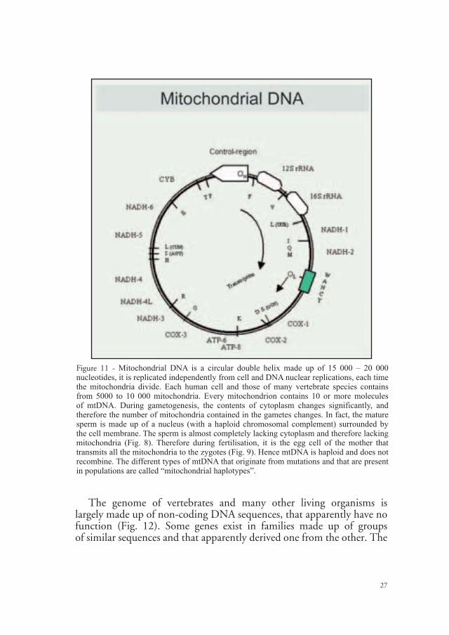
Mitochondrial DNA is generally circular in shape (Fig. 11). It is a circular double helix made up of 15 000 - 20 000 nucleotides, depending on the species. Mitochondrial DNA (mtDNA) is replicated, independently from cell and DNA nuclear replications, each time the mitochondria divide. Each human cell and those of many vertebrate species contains from 5000 to 10 000 mitochondria. Every mitochondrion contains 10 or more molecules of mtDNA. During gametogenesis, the contents of cytoplasm changes significantly, and therefore the number of mitochondria contained in the gametes changes. Mitochondria are provide entirely by the cell eggs. Therefore during fertilisation, it is the egg cell of the mother that transmits all the mitochondria to the zygotes. Hence mtDNA is haploid and does not recombine. The different types of mtDNA that originate from mutations and that are present in populations are called “mitochondrial haplotypes”.

Figure 10 - During meiosis, the chromosomes of every each pair, of which one is of maternal origin and the other of paternal origin, are paired and can exchange fragments through the genetic phenome-non of crossing-over. Crossing-over produces recombination. Recombination is an important process of genetic variability generation, as it produces new sequences of nucleotides that originate from the assortment of DNA segments, inherited partly from the mother and partly from the father.

27

The genome of vertebrates and many other living organisms is largely made up of non-coding DNA sequences, that apparently have no function (Fig. 12). Some genes exist in families made up of groups of similar sequences and that apparently derived one from the other. The

Figure 11 - Mitochondrial DNA is a circular double helix made up of 15 000 – 20 000 nucleotides, it is replicated independently from cell and DNA nuclear replications, each time the mitochondria divide. Each human cell and those of many vertebrate species contains from 5000 to 10 000 mitochondria. Every mitochondrion contains 10 or more molecules of mtDNA. During gametogenesis, the contents of cytoplasm changes significantly, and therefore the number of mitochondria contained in the gametes changes. In fact, the mature sperm is made up of a nucleus (with a haploid chromosomal complement) surrounded by the cell membrane. The sperm is almost completely lacking cytoplasm and therefore lacking mitochondria (Fig. 8). Therefore during fertilisation, it is the egg cell of the mother that transmits all the mitochondria to the zygotes (Fig. 9). Hence mtDNA is haploid and does not recombine. The different types of mtDNA that originate from mutations and that are present in populations are called “mitochondrial haplotypes”.

28

mechanisms that generate families of genes are called duplication and genetic conversion. The pairs of a duplicated gene start to evolve independently and accumulate different mutations. The effect of these mutations can be twofold: the duplicated gene remains active and acquires new functions (for example, it codes for a new protein), or else it is inactivated by the mutations that block its functionality. In this case the pair becomes a pseudogene. There are other families of repeated sequences that are probably generated by reverse transcriptase processes. RNA molecules are present in cells that are transcribed in DNA (through an enzyme, analogous to DNA polymerases, that are called reverse polymerases) and are in turn inserted into the chromosomes. This DNA seems to have an exogenous origin, for example it could derive from the reverse transcriptase of viral RNA. Once inserted into the genome, these sequences evolve by gene duplication. Currently, it is not clear whether these sequences have a certain function or whether they are simply made

Figure 12 - The genome of vertebrates and many other living organisms is largely made up of non-coding DNA sequences, that apparently have no function. Some genes exist in families made up of groups of similar sequences and that apparently derived one from the other. Repetitive DNA includes: satellite DNA, minisatellites (Fig. 14) and microsatellites (Fig. 15).

29

up of parasitic DNA which, once inserted into the genome, simply auto-preserve themselves by duplicating themselves incessantly without damaging the host genome. However recent data illustrates that certain repeated sequences do have a certain function, for example as crossing-over and recombination regulation sites.

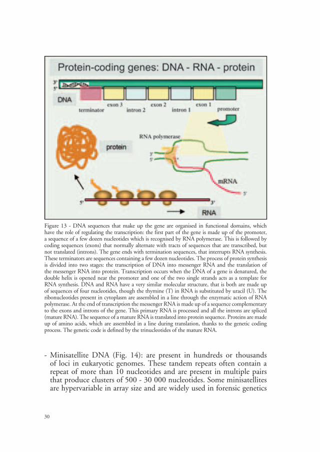
Genes, sequences present in a single copy or in a families made up of a small number of copies of the same gene, constitute the functional, non-repetitive DNA and codify for proteins (Fig. 13). DNA sequences that make up the gene are organised in functional domains, have the role of regulating the transcription: the first part of the gene is made up of the promoter, a sequence of a few dozen nucleotides which is recognised by RNA polymerase. This is followed by coding sequences (exons) that normally alternate with tracts of sequences that are transcribed, but not translated (introns). The gene ends with termination sequences, that interrupts RNA synthesis. These terminators are sequences containing a few dozen nucleotides. The process of protein synthesis is divided into two stages: the transcription of DNA into messenger RNA and the translation of the messenger RNA into protein. Transcription occurs when the DNA of a gene is denatured, the double helix is opened near the promoter and one of the two single strands acts as a template for RNA synthesis. DNA and RNA have a very similar molecular structure, that is both are made up of sequences of four nucleotides, though the thymine (T) in RNA is substituted by uracil (U). The ribonucleotides present in cytoplasm are assembled in a line through the enzymatic action of RNA polymerase. At the end of transcription the messenger RNA is made up of a sequence complementary to the exons and introns of the gene. This primary RNA is processed and all the introns are spliced (mature RNA). The sequence of a mature RNA is translated into protein sequence. Proteins are made up of amino acids, which are assembled in a line during translation, thanks to the genetic coding process. The genetic code is defined by the trinucleotides of the mature RNA.

Non-coding, tandemly repeated DNA exists in the genome of every species (repetitive DNA). Tandemly repetitive sequences, commonly known as “satellite DNAs” are classified into three major groups:

- Satellite DNA: highly repetitive sequences with very long repeat lengths (up to 5 000 000 nucleotides) that are usually associated with centromeres (the areas to which the fibres of the mitotic fuse attach themselves and that control the repartition of chromosomes in the two daughter cells during every somatic and gametic division). The satellite DNA is not used in population genetics or in forensic genetics.

30

- Minisatellite DNA (Fig. 14): are present in hundreds or thousands of loci in eukaryotic genomes. These tandem repeats often contain a repeat of more than 10 nucleotides and are present in multiple pairs that produce clusters of 500 - 30 000 nucleotides. Some minisatellites are hypervariable in array size and are widely used in forensic genetics

Figure 13 - DNA sequences that make up the gene are organised in functional domains, which have the role of regulating the transcription: the first part of the gene is made up of the promoter, a sequence of a few dozen nucleotides which is recognised by RNA polymerase. This is followed by coding sequences (exons) that normally alternate with tracts of sequences that are transcribed, but not translated (introns). The gene ends with termination sequences, that interrupts RNA synthesis. These terminators are sequences containing a few dozen nucleotides. The process of protein synthesis is divided into two stages: the transcription of DNA into messenger RNA and the translation of the messenger RNA into protein. Transcription occurs when the DNA of a gene is denatured, the double helix is opened near the promoter and one of the two single strands acts as a template for RNA synthesis. DNA and RNA have a very similar molecular structure, that is both are made up of sequences of four nucleotides, though the thymine (T) in RNA is substituted by uracil (U). The ribonucleotides present in cytoplasm are assembled in a line through the enzymatic action of RNA polymerase. At the end of transcription the messenger RNA is made up of a sequence complementary to the exons and introns of the gene. This primary RNA is processed and all the introns are spliced (mature RNA). The sequence of a mature RNA is translated into protein sequence. Proteins are made up of amino acids, which are assembled in a line during translation, thanks to the genetic coding process. The genetic code is defined by the trinucleotides of the mature RNA.

31

to obtain DNA fingerprinting. Profiling of these loci is done using multi-locus probes (MLP). Through molecular analysis, several loci that make up minisatellites have been identified (VNTR loci). These loci can be individualised and profiled through the use of specific probes (single -locus probes - SLP).

- Microsatellite DNA (Fig. 15): present in many thousands of loci in eukaryotic genomes. Microsatellites are made up of very short repeats (from 2 to 8 nucleotides) that are repeated only a few times and produce clusters of a few dozen or few hundred nucleotides at every locus. Microsatellites are used extensively in forensic genetics and are profiled through PCR.

The different categories of functional or non-functional tandemly repeated DNA evolve through different mutational processes that are associated with DNA structure and function.

Figure 14 - Minisatellite are present in hundreds or thousands of loci in eukaryotic genomes. These tandem repeats often contain a repeat of more than 10 nucleotides and are present in multiple pairs that produce clusters of 500 – 30 000 nucleotides. Some minisatellites are hypervariable in array size and are widely used in forensic genetics to obtain DNA fingerprinting. Profiling of these loci is done using multi-locus probes (MLP).

32

Figure 15 - Microsatellites are present in many thousands of loci in eukaryotic genomes. Microsatellites are made up of very short repeats (from 2 to 8 nucleotides) that are repeated only a few times and produce clusters of a few dozen or few hundred nucleotides at every locus. Microsatellites are used extensively in forensic genetics and are profiled through PCR. The lower part of this figure shows the structure of four different microsatellite alleles, and the results of their electrophoretic separation.

33

- Nucleotide and amino acid substitution (Fig. 16). The simplest type of mutation is the substitution of a nucleotide with another at a certain point in the DNA strand. Nucleotide substitutions are also called point mutations. A point mutation can occur in the non-coding regions of genes. The mutations that do not change the amino acid sequences are the so-called silent (synonymous) mutations. Mutations that modify the genetic code and cause amino acid substitution are non-synonymous mutations.

Figure 16 - Mutations. The simplest type of mutation is the substitution of a nucleotide with another at a certain point in the DNA strand. Nucleotide substitutions are also called point mutations. A point mutation can occur in the non-coding regions. The mutations that do not change the amino acid sequences are the silent (synonymous) mutations. Mutations that modify the genetic code and cause amino acid substitution are non-synonymous mutations. Insertion or deletion of a single nucleotide or a series of nucleotides can modify the reading frame of the gene-tic code or inactivate the gene. Crossing-over can be either symmetrical (Fig. 10) or asymmetrical. Asymmetrical crossing-over occurs more frequently between sequences of satellite or minisatellite DNA, that is, between tandemly repeated DNA that do not align themselves precisely. Asymme-trical crossing-over gives rise to the deletion of a DNA fragment from a chromatid and its inser-tion into another chromatid. Asymmetrical crossing-over may occur between two chromatids of the same chromosome or between two different chromosomes.

34

- Insertion or deletion of a single nucleotide or a series of nucleotides (Fig. 16). These mutations can modify the reading frame of the genetic code or inactivate the gene.

- Crossing-over and recombination. Crossing-over can be either symmetrical (Fig. 10) or asymmetrical (Fig. 16). Symmetrical crossing-over produces exchanges of corresponding sequences between two chromosomes and produces genetic recombination (Fig. 17). Asymmetrical crossing-over occurs more frequently between sequences of satellite or minisatellite DNA, that is, between tandemly repeated DNA that do not align themselves precisely. Asymmetrical crossing-over gives rise to the deletion of a DNA fragment from a chromatid and its insertion into another chromatid. Asymmetrical crossing-over may occur between two chromatids of the same chromosome or between two different chromosomes.

- DNA slippage (Fig. 18). Slippage occurs during replication when the nascent DNA separates and reassociates itself temporarily from the DNA template. During replication of non-repetitive sequences, the possible disassociation of the sister chromatid does not usually generate mutations, because the nascent DNA can reassociate only and exactly in the complementary point of the DNA template. Instead, during tandemly repeated DNA replication, the single strand nascent DNA can pair in another point of the DNA template. When replication continues, the nascent DNA is found to be longer or shorter than the template.

- Gene conversion (Fig. 19). Gene conversion produces the transfer of a DNA sequence from one allele to another.

Genetic mutations and polymorphisms

Mutations generate genetic variability in individuals and populations. A variable gene is defined as polymorphic. Polymorphisms indicate the presence of two or more variants of a DNA sequence. Obviously, gene coding polymorphisms can generate protein polymorphisms (for example, alloenzymes, blood groups, immunoglobulins, etc), apart from phenotype polymorphisms (colour of the eyes, skin, hair structure, fingerprints, etc). All these characters can be used as markers in the identification and individualisation of samples in forensic science. The highly variable non-coding DNA sequences, that apparently are not subjected to strong pressure from natural selection and therefore evolve

35

rapidly and neutrally, make up the most useful and reliable genetic markers in acquiring evidence in forensic genetics.

Mutations in minisatellites. Minisatellites are hypervariable, with mutation rates reaching 10¯3 per fragment per gamete. Every allele muta-tes once in about every thousand cycles of gametogenesis, which means that one can expect to find a mutation at every gametogenesis analysing

Figure 17 - Crossing-over and recombination. Symmetrical crossing-over produces exchanges of corresponding sequences between two chromosomes and produces genetic recombination.

36

about a thousand independent alleles in a multi-locus profile. These rates of mutation generate the large number of alleles that are necessary for individualisation, but can also generate aspecific fragments that are dif-

Figure 18 - Slippage occurs during replication when the nascent DNA separates and reassociates itself temporarily from the DNA template. During replication of non-repetitive sequences, the possible disassociation of the sister chromatid does not usually generate mutations, because the nascent DNA can reassociate only and exactly in the complementary point of the DNA template. Instead, during tandemly repeated DNA replication, the single strand nascent DNA can pair in another point of the DNA template. When replication continues, the nascent DNA is found to be longer or shorter than the template.

37

ficult to assign. For example, pos-sible somatic mutations can gene-rate different DNA fingerprints in DNA samples extracted from dif-ferent tissues of the same indivi-dual. In this case, identification could be problematic. Moreover, gametic mutations can generate differences between parents and offspring. In both cases these muta-tions could generate false negati-ves and therefore produce a false exclusion diagnosis. However, in the space of a generation, these mutations are always rare, and in practice should not interfere in results of genetic analysis. A paren-tal test is based on the analysis of

multi-locus profiles transmitted from parents to offspring in a genera-tion. With mutation rates in the order of 10-3 per fragment per gamete, there would be a probability of finding a mutation if the maternal pro-file was composed in total of a thousand diagnostic alleles. In parental testing, 20 to 40 fragments for every pair of parents are used, therefore the probability of a new mutation remains quite small. Moreover, a soma-tic or gametic mutation would modify the profile of a single fragment or of a single allele in a multi-locus system. For example, if on the basis of data obtained from a single locus, an allele that was not present in the putative father appears following a mutation in the offspring’s profile, that father could be incorrectly excluded. It is very unlikely that other mutations modified the profiles of other independent loci contempora-neously, or in multi-locus profiles obtained by using other restriction enzymes. Hence a single mutation cannot be used as proof of exclusion. The significance of a single mutation must be evaluated by analysing dif-ferent loci in single locus systems, or utilising two or more restriction enzymes in multi-locus systems.

Mutations in microsatellites. Microsatellites are sequences made up of a simple motif of 2-8 nucleotides, that is repeated in tandem for a certain number of times, with or without interruptions due to the insertion of

Figure 19 - Gene conversion. Gene conversion produces the transfer of a DNA sequence from one allele to another.

38

other nucleotides or other sequences. Microsatellites have high levels of polymorphism. Microsatellites have been identified in the genome of all organisms analysed up to now, and are distributed in a more or less random way in chromosomes. They are not usually present in coding sequences of genes (exons), while they may be present in introns. The composition of microsatellites sequences is variable: the poli(A)/poli(T) motifs are very common in vertebrates, but cannot be used as genetic markers because they are extremely unstable during PCR. The CA/GT motifs are among the most common dinucleotides. Other dinucleotides are AT/TA and AG/TC. Then there are microsatellites made up of repeated sequences of trinucleotides (for example CAG, or AAT) or even tetranucleotides. In some cases the flanking sequences are preserved in the course of evolution. It is possible to use conserved PCR primers to amplify and analyse microsatellites in different species. Mutations that determine an addition or a loss of one or more repeat units are much more frequent than nucleotide substitutions. The estimated mutation rates in microsatellites of invertebrates are 10-4 - 10-5 mutations per locus for every generation. These mutations are therefore one or two orders of magnitude less than the mutation rate of minisatellites. The mutation processes that determine the variation in the number of repeats and therefore the variation of the molecular weight of the alleles at microsatellite loci is slippage and asymmetrical crossing-over. Some experimental results suggest that slippage is probably the main mechanism responsible for mutations of microsatellites.

Nucleotide substitution. DNA sequences of exons are preserved by natural selection, that eliminates all those mutations that produce malfunctioning proteins or that impede protein synthesis. However the genetic code is degenerated, that is, there are more triplet nucleotides (codons) that codify for the same amino acid. Redundancy is caused particularly by the nucleotide in third position in every codon. Hence, many nucleotide substitutions that occur in the third position of condons are synonymous. Synonymous mutations are much more frequent than non-synonymous nucleotide substitutions. Nucleotide substitutions and rearrangements (insertions and deletions) are much more frequent in non-coding DNA sequences and in repetitive DNA. In particular, DNA sequences in the control-regions in mtDNA replication are much more variable. Nucleotide sequences of non-coding DNA, introns and above all the control-region of mtDNA, are hypervariable in populations and are used in forensic genetics.

39

GENETIC VARIABILITY IN INDIVIDUALS AND POPULATIONS

The process of heredity: Mendel’s laws

Studies by Gregor Mendel published in 1866 gave rise to modern genetics. In his experiments, Mendel used pure lines of pea plants that displayed well identified phenotype characters. For example, some lines always had yellow seeds, while in others the seed colour was green. Mendel carried out experiments of cross-fertilisation, describing the frequency of the phenotype characters that appeared in successive generations of crosses and backcrosses, and developed a genetic model that could explain the results of hybridisation. The objective of Mendel’s experiments was to determine the laws that control the hereditary transmission of phenotype “characters”. Mendel hypothesised that the phenotype expression of each character was determined by discrete “genetic factors”, that later would be called “genes”, that are transmitted unaltered in the course of generations from parents to their offspring. For example, from cross-fertilisation between two pure parental lines of peas, one with green seeds and the other with yellow seeds, Mendel obtained a first generation (F1) that displayed 100% yellow seeds, due to the effect of the dominating yellow character over the green character. By cross breeding F1 plants among themselves, Mendel obtained a successive generation (F2) in which the green seed character reappeared, though it had apparently disappeared in F1, with a frequency that is precisely foreseeable if the Mendelian model of heredity is applied (Fig. 20).

Mendel’s first law, the “law of independent segregation of the alleles”, established that during meiosis, the two alleles are separated (segregated) independently in different haploid cells. Mendel’s second law, the “law of independent assortment of different genes”, establishes that alleles found at different loci, placed on different chromosomes are associated (assorted) independently during meiosis. Mendel’s law allows one to estimate the proportion of different genotypes that are produced with each generation, as a simple and direct consequence of segregation and independent assortment of the alleles in one or more loci (Fig. 21).

Today we know that every individual inherits one chromosome of every pair from the mother and one from the father. Each gene is placed at a particular location of the chromosome (“locus”, plural “loci”), and is present in two forms, each of which is called “allele” (Fig. 4). The location of the gene loci in the chromosomes allows the chromosomal map to be traced. The identification of the alleles present at polymorphic loci

40

allow individual genotypes to be identified and to estimate the genetic variability in populations. Two alleles at a particular location can have identical genetic characteristics (the locus is “homozygous”) or else possess different characteristics (the locus is “heterozygous”; Fig. 17). In this case the locus is "polymorphic". Alternatively, the locus is called "monomorphic". A diploid individual can have two different alleles (at

Figure 20 – A Mendelian cross. Cross-fertilisation between two pure parental lines of peas, one with green seeds and the other with yellow seeds. The first generation (F1) displayed 100% yellow seeds, due to the effect of the dominating yellow character over the green character. By cross breeding F1 plants among themselves, Mendel obtained a successive generation (F2) in which the green seed character reappeared, though it had apparently disappeared in F1, with a frequency that is precisely foreseeable if the Mendelian model of heredity is applied.

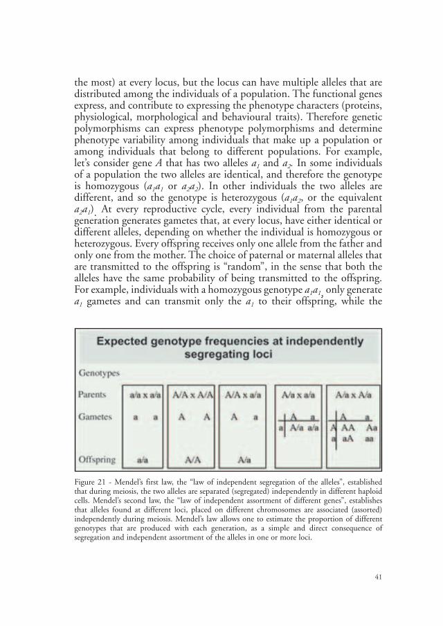
41

the most) at every locus, but the locus can have multiple alleles that are distributed among the individuals of a population. The functional genes express, and contribute to expressing the phenotype characters (proteins, physiological, morphological and behavioural traits). Therefore genetic polymorphisms can express phenotype polymorphisms and determine phenotype variability among individuals that make up a population or among individuals that belong to different populations. For example, let’s consider gene A that has two alleles a1 and a2. In some individuals of a population the two alleles are identical, and therefore the genotype is homozygous (a1a1 or a2a2). In other individuals the two alleles are different, and so the genotype is heterozygous (a1a2, or the equivalent a2a1). At every reproductive cycle, every individual from the parental generation generates gametes that, at every locus, have either identical or different alleles, depending on whether the individual is homozygous or heterozygous. Every offspring receives only one allele from the father and only one from the mother. The choice of paternal or maternal alleles that are transmitted to the offspring is “random”, in the sense that both the alleles have the same probability of being transmitted to the offspring. For example, individuals with a homozygous genotype a1a1, only generate a1 gametes and can transmit only the a1 to their offspring, while the

Figure 21 - Mendel’s first law, the “law of independent segregation of the alleles”, established that during meiosis, the two alleles are separated (segregated) independently in different haploid cells. Mendel’s second law, the “law of independent assortment of different genes”, establishes that alleles found at different loci, placed on different chromosomes are associated (assorted) independently during meiosis. Mendel’s law allows one to estimate the proportion of different genotypes that are produced with each generation, as a simple and direct consequence of segregation and independent assortment of the alleles in one or more loci.

42

heterozygous individuals (for example a1a2) generate gametes that are both a1 and a2, and can transmit both alleles a1 and alleles a2.

Mendel’s laws allow genotypes frequencies to be calculated even in populations that are not made up of pure lines (each of which consists of individuals that are identical for the character in question), but of individuals that present one or the other of the two forms, and that are found in the population at a certain frequency. For example, in a population made up of individuals reproducing randomly, in which at locus A (with two alleles a1 and a2) allele a1 is present with a frequency p = 0.60 (that is, that allele a1 is present in 60% of individuals and therefore in 60% of gametes), the frequency of the homozygous genotype a1a1 will simply be 0.60 x 0.60 = 0.36. Obviously, the frequency of allele a2 will be q = 1 - p = 0.40. Therefore, the frequency of the homozygous genotype a2a2 will be 0.40 x 0.40 = 0.16. The frequency of the heterozygous a1a2 will be 0.60 x 0.40 = 0.24, that is, equal to the frequency heterozygous a2a1. Hence, the total frequency of heterozygous will be 2 x 0.60 x 0.40 = 0.48. The proportions of the genotypes at locus A will therefore be = p² + 2pq + q² = 0.36 + 0.48 + 0.16 = 1.00.

Genotypes and genotype frequencies calculated on the basis of Mendel’s laws are still at the basis of parental testing today. For example, if a mother with a genotype a1a2 has a child with genotype a1a3 then allele a3 must have been transmitted by the father. In this case, the putative fathers with genotypes a1a1, a1a2 or a2a2, can be excluded as biological fathers of that child. A putative father that has allele a3 has a certain possibility of being the biological father. This probability can be estimated quantitatively using information on the allele a3 frequency in the population and using the appropriate statistical procedures.

The processes of heredity: association between genes (linkage)

Chromosomes are transmitted from parent to offspring as intact units, therefore the genes that are located on different chromosomes are inherited independently one from one another (random assortment). On the contrary, genes mapping near each other on the same chromosome tend to be inherited together and therefore exhibit genetic linkage. However, during meiosis, crossing-over produces recombinations that break the linkage groups (Fig. 17). The closer two genes are physically near each other on the chromosome, the more likely it is that they will be inherited as a single unit. Linkage is one of the exceptions to Mendel’s laws. When two loci are in linkage equilibrium (LE), the frequencies of all

43

the possible allelic combinations depend solely on the allele frequencies in the population. The frequencies of allelic combinations are obtained by calculating the product of the frequencies of all the possible alleles pairs. If certain allelic combinations are more frequent than expected, then the locus is in linkage disequilibrium (LD).

Let’s consider two loci: A (with two alleles a1 and a2) and B (with two alleles b1 and b2). The two loci reside on the same chromosome, but are not near one another. Every individual can have one of the following genotypes at locus A: a1a1, a1a2 or a2a2; and at locus B: b1b1, b1b2 or b2b2. Considering the two loci together, it is possible to generate nine different groups:

a1a1, b1b1

b1b2

b2b2

a1a2, b1b1

b1b2

b2b2

a2a2, b1b1

b1b2

b2b2

These genotypes can generate four possible types of gametes (haplotypes):

a1 b1

a1 b2

a2 b1

a2 b2

The individuals that are homozygous at both loci (double homozygotes) can only transmit one type of gamete (for example, a1a1, b1b1 can only transmit the haplotype a1 b1). Homozygous individuals at only one locus can transmit two types of gametes (for example, a1a1, b1b2 can transmit the haplotyes a1a1 and b1b2). The double heterozygotes a1a2, b1b2 can transmit only two types of gametes, that is, two parental haplotypes, for example a1b1, and a2b2, in the absence of recombination, or four types of gametes, and that is, two parental haplotypes plus two recombinant hapotypes, a1b1, a1b2, a2b1 and a2b2, in the presence of recombination. If the probability of recombination is c, every recombinant gamete is transmitted with probability c/2 and every parental gamete with probability (1 - c)/2. All the loci that reside on different chromosomes are not associated, segregate independently and therefore transmit four

44

gametic haplotypes with equal probability. The double heterozygotes at these loci produce four types of gametes with equal probability, corresponding to c = 0.5. Therefore, the values of c are comprised between a minimum of c = 0.0 (for pairs of loci near each other on the same chromosome, with no probability of recombination) and c = 0.5 (for pairs of loci that reside on different chromosomes and that segregate in a completely independent manner). Linkage disequilibrium (LD) indicates that the probability that an individual inherits an allele at locus A, also depends on the probability that it inherits an allele at locus B. The LD coefficient between alleles a1 and b1 is given by the difference between the frequency observed of the haplotype a1b1, p(a1b1), and its expected frequency, that corresponds to the product of the two allele frequencies p(a1) and p (b1):

LD = p(a1 b1) - p(a1) p (b1)

For example, if the allele frequencies are:

a1 = 0.9a2 = 0.1b1 = 0.6b2 = 0.4

the expected frequencies of the four gametic combinations are:

a1 b1 = 0.54a1 b2 = 0.36a2 b1 = 0.06a2 b2 = 0.04

If the observed frequencies of these four haplotypes are different, and certain combinations are more frequent than expected, then it is possible that a linkage disequilibrium exists. The meaning of this discrepancy between the frequencies observed and expected can be determined through appropriate statistical analysis, including the chi-square significance test.

In forensic genetics, it is important to utilise independent loci that are not in LD in the reference population. In fact, the basic procedures to find multi-locus genotype frequencies starting from the allele frequencies at single loci is based on the product rule that requires independence of the factors (the loci).

LD can be produced by recent mutations that have not yet been randomised through genome recombination, or through natural selection,

45

which favours the permanence of certain allelic combinations that have functional and adaptive roles. A population subject to migration, or which originated from the admixture of two genetically distinct subpopulations, can be in linkage disequilibrium, even if both subpopulations are in linkage equilibrium. The value of LD in mixed populations is proportional to the differences between the allele frequencies of the two subpopulations. One can demonstrate that:

LD = mImII (p(a1)I - p(a1)II)(p(b1)I - p(b1)II)

With p(a1) and p(b1) = allele frequencies in subpopulations I and II; mI and mII = proportion of the two subpopulations in the total population.

In theory, LD is eliminated rapidly through recombination. The value of LD declines in the course of generations, with a rate of decline from one generation to the next that corresponds to:

LD’ = (1 - c)LD

The decline of LD is at its greatest if c = 0.5, that is if the genes are not linked. In the case of mixed populations LD declines to LD’ = (1 - 0.5)LD = 0.5LD, that is, it is halved after the first generation of random reproduction in the subpopulations.

Genes in populations

The aim of population genetics is to describe the genetic composition of populations and to understand the causes that determine changes (evolutionary forces). Every species is made up of one or more populations that contain a certain quantity of genetic variability, originating from mutations, that cause the disappearance of numerous alleles at different loci. Genetic variability in populations is described through allele frequencies. Allele frequencies at each locus can vary in the course of generations due to mutations, natural selection, migration or genetic drift. The different combinations of alleles present at each locus determine individual genotypes, whose frequency in populations can be calculated. In an ideal population, in which evolutionary forces are not active, genotype frequencies remain constant from one generation to the next. Population genetics is based on an abstract, ideal population model, supported by a series of assumptions. The model must be simple, in such a way to render mathematical analysis possible, but consequently will not be very realistic. Every model must reach a compromise between

46

simplicity and reality. In genetics, the ideal population has infinite size, the individuals mate and reproduce “at random”, that is, every individual has the same probability to reproduce with any other individual of the population and the mating choice of an individual is not influenced by the mating choice of other individuals. Real populations have finite size and can be considered replicates of an ideal population, that differ one from another according to the number (finite) of alleles of the ideal population (infinite) that were included in every random sampling (genetic sampling). In practice, we analyse samples of limited size (the size of the sample is indicated by n) that were obtained through genetic sampling of real populations. These samples are different from each other because of the limited number of individuals that are effectively sampled each time (statistic sampling). The Hardy-Weinberg law (1909) defines the relationship that exists between allele and genotype frequencies at each locus in a population. It states that in a Mendelian population, the proportion of genotypes remains constant from one generation to the next. In a locus with two alleles (a1 and a2), with frequencies p and q, with p + q = 1, the genotype frequencies are obtained from the proportion: a1a1:2a1a2:a2a2 = p2:2pq:q2. The Hardy-Weinberg proportions can be found simply from analysing a table that contains the results of all the possible combinations between maternal and paternal genotypes present in a Mendelian population at a polymorphic locus with two alleles (Fig. 22).

It is possible to estimate the genotype frequencies of a population in Hardy-Weinberg equilibrium (HWE) using the observed allele frequencies. For example, if we know that allele a1 has a frequency p = 0.2, then the genotype frequencies will be:

homozygous genotype: p(a1a1) = p2 = (0.2 x 0.2) = 0.04heterozygous genotype: p(a1a2) = 2pq = 2 x (0.2 x 0.8) = 2 x 0.16 = 0.32

Obviously, the estimated genotype frequencies, calculated through allele frequencies, are representative of the genotype frequencies of the population, only if the population is in HWE. The same Hardy-Weinberg law states that genotype and allele frequencies do not change after the first generation of random reproduction. The population is, and remains in HWE equilibrium after a generation and for all the following generations, in the absence of evolutionary forces. However, in certain cases a population remains in HWE equilibrium even if there is a certain pressure of natural selection or if a proportion of mating does not occur randomly.

47

In calculating the genotype frequencies, one applies the product law, which implies that every event is random and independent from another. If a population is not in HWE (something that may evaluate by applying the chi-square test) an estimate of the genotype frequencies, starting from the allele frequencies, may be wrong. Deviations from HWE may be caused by non-random mating, gene flow, founder effect, bottleneck and random drift.

Figure 22 - The Hardy-Weinberg equilibrium in a population with two alleles (a1 and a2), with frequencies p and q, with p + q = 1, at a locus A. The genotype frequencies are obtained from the proportion: a1a1:2a1a2:a2a2 = p2:2pq:q2.

48

In forensic genetics, either non-coding DNA sequences or DNA tandem repeats are usually used. The effects of natural selection on these sequences are usually irrelevant. Moreover, the aim of forensic genetic analysis is to establish correspondences between a sample and an individual from which the sample derived, or to establish the parental relationship in family nuclei. In these cases the effects of mutations are irrelevant. On the contrary, the consequences of migration and reduction in population size could have important consequences, determining mixed populations or populations with high levels of inbreeding, that can be in Hardy-Weinberg disequilibrium (HWD).

Migration and the admixture of differentiated populations, causes stratified populations that are genetically heterogeneous. If a population is subdivided into genetically distinct subgroups, with random reproduction within the subgroups, but with a limited gene flow among them, then it is possible to calculate the allelic and genotype frequencies separately in the subgroups. Otherwise the frequencies are calculated in the mixed population. If the allele frequencies are different in the subgroups, then the total population may be in HWD. This phenomenon is known as the Wahlund Effect: the homozygosity observed in a population made up of subgroups that have recently admixed and that are not panmitic, is significantly higher than the homozygosity estimated on the basis of HWE in the total population. Methods to analyse admixed populations that identify the subgroups present and assign every individual to the subpopulation of origin are available (Pritchard et al. 2000).

Inbreeding

Individuals of a real population can reproduce non-randomly because they choose each other on the basis of certain phenotypes, behavioural and social criteria (non-random mating), or else because they are related. Reproduction between individuals that are related is called “inbreeding”. In real populations, all individuals are in some way related, if one goes back a certain number of generations. However, conventionally, two individuals are considered inbred if they derive from parents related to each other in the previous three or four generations. The consequences of non-random mating and inbreeding are similar: an increase in frequency of the homozygous individuals in the population. Therefore, homozygosity increases with respect to a population that is in HWE. In forensic genetics it may be important to know the degree of kinship among the individuals analysed, because inbreeding can significantly change the probability of identity between two genotypes.

49

Inbreeding in individuals. Two individuals who have a recent ancestor in common are related and their offspring are “inbred”. The genetic consequences of inbreeding derive directly from Mendel’s laws. Every individual receives half its alleles from each parent and transmits half of the alleles to each of the offspring. The probability of receiving or transmitting one or the other of the two alleles present at each locus is the same. An individual born from two related parents has a certain probability of receiving both the alleles at a locus that are copies of the same alleles, that is, they are identical by descendence (identity by descent: ibd). The probability that an individual receives copies of the ibd alleles from his/her parents corresponds to the “inbreeding coefficient” F. Hence, F is an estimate of the probability of homozygosity due to ibd alleles. It is possible to estimate the individual inbreeding coefficient by assuming that an initial reference population exists, in which all the individuals are not inbred. If all the births that occurred in this population have been registered, then a “pedigree” exists which can be used to calculate the individual values of F. For example, the inbreeding of an individual born from the union of two brothers, that have both their parents in common, is F = 0.25, equivalent to the probability that the individual receives a pair of alleles ibd (Fig. 23). Inbreeding of an individual born from the union of two half-brothers, that have only one parent in common, is F = 0.125 (Fig. 24).

Methods exist which, when implemented in computer programmes, allow the individual values of F to be established, through the analysis of complex pedigrees. In the case of a simple pedigree, the inbreeding coefficient values between pairs of related individuals can be found directly from table 1.

The coancestry coefficient (θ) is another measure of inbreeding, that corresponds to the probability that two alleles at a locus in two individuals taken at random from the population are ibd. The inbreeding coefficient F estimates the probability that an individual randomly chosen from the population receives two ibd alleles for every locus; the coancestry coefficient θ estimates the probability that two individuals randomly chosen have two ibd alleles, and therefore it is a measurement of inbreeding among individuals. The inbreeding coefficient F and the coancestry coefficient θ are correlated. If two individuals, X and Y have an offspring I, FI = θXY, that is, the inbreeding coefficient of the offspring corresponds to the coancestry coefficient between his/her parents, because the probability that a locus of the offspring is homozygous for ibd alleles is the same as the probability that his/her parents have two ibd alleles per

50

locus. Therefore, θ = 1/4 for the offspring of the two brothers (that have F = 0.25), 1/8 for the offspring of two half-brothers (that have F = 0.125) and 1/16 for the offspring of two first cousins (that have F = 0.0625).

Inbreeding in populations. In a population, the average inbreeding coefficient corresponds to the probability that two alleles at a locus of a randomly chosen individual is ibd. In a population of finite size there is a probability that increases with time that a pair of alleles are ibd, simply because with every generation some alleles are not transmitted to the following generation, while others are transmitted in multiple copies. If a population has inbreeding F, what will the value of F be in the following generation? Let’s assume we have a population made up of N individuals. The probability that an individual of the following generation has two distinct parents is 1 - 1/N and the probability of receiving two ibd alleles

Figure 23 – The inbreeding coefficient of an individual born from the union of two brothers, that have both their parents in common, is F = 0.25.

51

correspond to the valore of θ. One can demonstrate that after one generation, the inbreeding coefficient of the populations will be:

F’ = θ’ = 1/2N + (1 - 1/2N)θTo the generation t:

θt = 1 - (1 - 1/2N)t

In figure 25 the values of F = θ are shown for t generations of populations of N = 100 000, 10 000, and 1000 individuals

Figure 24 - The inbreeding coefficient of an individual born from the union of two half-brothers, that have only one parent in common, is F = 0.125.

Table 1 - Inbreeding coefficient.

Relationship Degree F

Monozygotic twins IdenticalDizygotic twins First 1/4Brothers First 1/4Parents - child First 1/4Uncle - nephew Second 1/8Half - brothers Second 1/8First cousins Third 1/16Second cousins Fifth 1/64

52

(from Evett and Weir, 1998). The increase of inbreeding is accompanied by a decrease in genetic variability in the population, due to drift. Clearly, both the increase of F and the decrease of genetic variability are slight in case of large N. Inbreeding will reach the values of 1 after about 10 000 generations in a population of N = 1000 individuals, and after about 10 000 000 in a population of N = 100 000.

It is necessary to state that N is the “effective size” of the population, that corresponds to the number of individuals that actually reproduce and that transmit their genes to following generations. The effective population is almost always much smaller or very much smaller than the surveyed size, that is, the number of individuals that are present in the population. This occurs because not all the individuals in a population fall within the reproductive age at the same time, the sex ratio of reproductive individuals does not always correspond to one male for

Figure 25 - Values of F = θ are shown for t generations of populations of N = 100 000, 10 000, and 1000 individuals. The increase of F is slight in case of large N. Inbreeding will reach the values of 1 after about 10 000 generations in a population of N = 1000 individuals, and after about 10 000 000 in a population of N = 100 000.

53

each female, fertility and fecundity of individuals are not identical, the survival of siblings is not identical, and so on. The effective size can be 2 to 20 times lower than the observed size of the population. Small and isolated populations (that do not receive “immigrants”) are subject to “genetic drift”: the allele frequencies fluctuate from one generation to the next. In the long term, drift produces a loss of alleles and therefore a decrease of genetic variability in the population. In fact, random fluctuations of allele frequencies cause loss of alleles, with the consequent fixing of alternative alleles. The fixed loci become monomorphic and the value of heterozygosity is reduced to zero.

Drift inevitably produces an increase of F in real populations, which always have finite size and in effect, are often smaller in size than the observed size. To make the population genetic model more realistic, it may be opportune to express the estimated HWE genotype frequencies, both in terms of allele frequency and the inbreeding coefficient. Inbreeding causes an increase in homozygous genotype frequencies and a decrease in heterozygous genotype frequencies, that is, a decrease of heterozygosity H. A homozygous individual receives two pairs of the same allele a from his parents. However, in a finite population, there is a probability F that these allele a are ibd. The possibility that the a are non-ibd will consequently be = (1 - F). Therefore, the frequency of this genotype can be expressed as the estimated HWE frequency, weighed by a component due to drift (or due to any other cause that increases inbreeding). The inbreeding coefficient F measures the decrease of H with respect to the estimated heterozygosity of a population in HWE, that is:

F = (2pq - H)/2pq

From which the following derives:

H = 2pq(1 - F).

In an inbred population the estimated frequencies of three genotypes at a locus with two alleles are:

p(a1a1) = Fp + (1 - F) p2

p(a1a2) = 2pq(1 - F) p(a2a2) = Fq + (1 - F) q2

For example: if allele a1 has frequency p = 0.05, the frequency of the homozygous genotype in a population in HWE will be p2 = 0.0025. However, in a group of individuals born from mating cousins, with F = 1/16 and (1 - F) = 15/16, the homozygous frequency will be:

54

1/16 x 0.05 + 15/16 x 0.0025 = 0.003 + 0.0023 = 0.0053

that is, it will be more than doubled with respect to a population in HWE.

If the population is in HWE and F = 0 (there is no inbreeding), the three precedent equations become the same as the expected allele frequencies for the three genotypes: p2, 2pq, q2. On the contrary, if F = 1, the population will be made up exclusively of two homozygous genotypes with frequencies p and q, respectively.

From this model that calculates inbreeding, it is possible to develop more complex derivations. We can consider the relationship between pairs of related individuals, for example siblings, between individuals that belong to distinct subpopulations, etc. It is possible to estimate the probability that two non-inbred individuals have 0, 1, 2, etc. pairs of ibd alleles, the probability that individuals have two loci which are both homozygous, or that have a homozygous locus and a heterozygous one, or that they have the same or different heterozygous genotypes at two loci. Moreover, it is possible to estimate that probability that two related individuals derived from non-inbred and unrelated parents, have the same genotype.

MOLECULAR GENETICS:METHODS OF ANALYSING DNA VARIABILITY

The procedures of molecular analyses used in population genetics and forensic genetics consist in: collection and conservation of biological samples; DNA extraction; digestion of DNA through restriction enzymes; DNA fragment separation through electrophoresis in agarose or acrylamide gel; immobilisation of DNA fragments through Southern blotting; preparation of labelled nucleotide probes; hybridisation and identification of restriction fragments; DNA amplification through PCR; nucleotide sequencing; automated sequencing, microsatellite and DNA fragment analyses (Fig. 26).

Collection of biological samples

Molecular analysis techniques that are based on PCR require small quantities of DNA, and therefore any type of biological sample can be utilised. However, these techniques are greatly exposed to the risk of

55

Figure 26 - The procedures of molecular analyses used in population genetics and forensic genetics consist in: collection and conservation of biological samples; DNA extraction; digestion of DNA through restriction enzymes; DNA fragment separation through electrophoresis in agarose or acrylamide gel; immobilisation of DNA fragments through Southern blotting; preparation of labelled nucleotide probes; hybridisation and identification of restriction fragments; DNA amplification through PCR; nucleotide sequencing; automated sequencing, microsatellite and DNA fragment analyses.

56

contamination. Instead the more traditional techniques (for example, restriction fragment analysis) require greater quantities of DNA that can be obtained only from biological samples that are not too small or too degraded. In any case, analysis procedures and the quality of the results are dependent on the quality of the samples and possible contamination. It is therefore necessary to collect and preserve the biological samples in the best possible manner.

Samples of animal origin that are most commonly utilised are the following:

Blood samples taken from live animals. Nuclear DNA is extracted from white blood cells, that contain a nucleus, or from red blood cells of amphibians, reptiles and birds as they contain a nucleus. Mammals have anucleated red blood cells. Most mitochondrial DNA (mtDNA) is extracted from white blood cells. The necessary amount of DNA to perform molecular testing used in forensic genetics can be taken from 10 - 100 microlitres (µl) of amphibian, reptile, and bird blood, or else from about 0.5 - 1.0 millilitres (ml) of mammal blood. The mtDNA is present in multiple copies in the cytoplasm of white blood cells and can be extracted from a few µl of blood, no matter what species. Total DNA (that contains both mtDNA and DNA nuclear) is normally extracted from blood samples. Nuclear or mitochondrial genes are then selectively amplified through PCR, selectively individualised through the use of specific nucleotide primers. Blood can be extracted simply by pricking a vein and collecting the drops with a capillary, or with an insulin-type sterile syringe. The insulin type syringes can draw from a few µl up to 1 ml of blood, using a needle with a very small diameter. Blood can be taken from any vein that is easily accessible. It must be carried out with care, avoiding harmful consequences for the animal. In any case, this operation must be preceded by disinfecting the skin, and a new, sterile syringe and not a recycled one must be used. Blood sampling for CITES analyses must be carried out by a veterinarian chosen by the owner of the animals. The blood sampling costs are to be paid by the owners. Blood sampling may be carried out using anticoagulant solutions. EDTA bisodic salt (EDTA.Na2) is an anticoagulant solution that is recommended, as it does not interfere with sampling procedures nor DNA analysis. A few drops of a solution at 10% of EDTA.Na2 (obtained by dissolving 10 grams of EDTA.Na2 in 100 ml of warm, sterile double distilled water) are sufficient for a blood sample of 1 ml taken using an insulin syringe. Blood samples are preserved in Longmire buffer (LongBuffer).

57

Samples of solid tissue taken from living (via biopsies) or dead animals. Small biopsies, for example, taken from the ear, or else samples of about 0.5 - 2.0 gr of tissue taken from carcasses of dead animals, are sufficient to carry out DNA analysis. Tissue samples of any type must be preserved in sterile, plastic test tubes that are hermetically sealed, containing ethanol (ethyl alcohol) at 90-100% (EtOH 100%). It is extremely important to use pure ethanol, and not denatured ethyl alcohol. Denaturing substances, that colour the alcohol pink, can contaminate the DNA and make genetic analyses impossible. It is also extremely important to preserve the samples in volumes of ethanol al least 10 times greater than the tissue weight (for example, 1 gr of tissue must be preserved in at least 10 ml of ethanol). Ethanol dehydrates the tissues, and in this way blocks the biochemical reactions that could degrade the DNA. Tissues contain water that, during dehydration, dilutes the ethanol. Therefore to avoid excessive dilution, it is necessary to use abundant volumes of ethanol at 90 - 100%. DNA is stable in ethanol at room temperature. Hence, samples in ethanol can be preserved at room temperature or else refrigerated at any temperature inferior to room temperature. Dead animals to be used for DNA analysis must be immediately frozen and the bodies must be preserved at the lowest possible temperature. Freezing at temperatures of -10/-15°C normally guarantees the conservation of DNA for several months, while freezing at -80°C, or else in liquid nitrogen, allows DNA to be preserved for many years. In any case, it is important to know that freezing large animal bodies is a slow process, starting from the external surface inwards. DNA of internal tissues may be subject to decay if the freezing process is extended over a long time. It is worthy keeping in mind that freezers are subject to breakage and that electricity could be cut off. Prolonged and repeated defreezing of tissues produces DNA degradation. Hence, the necessary aliquot of tissue for genetic analysis should be taken as soon as possible rather than freeze the bodies for a long period. The aliquots of tissue to be used for genetic analysis must be preserved in ethanol. Biopsies and samples must be carried out with extreme caution avoiding contamination. It is necessary to work on clean surfaces, disinfecting or washing the parts of the body where samples are to be taken from, using clean, sterilised (the disposable type) scalpels, scissors and forceps, and avoid touching samples with fingers unless wearing sterile, latex, laboratory gloves.

Hair and feather samples. Sufficient quantities to carry out DNA analyses can be obtained through PCR, using the cells that are present in hair bulbs and quills (roots) of feathers. In this case it is necessary to

58

take 10-20 hairs with bulbs, or else 2-4 feathers or feather down from each specimen. They must be extracted using laboratory gloves, or with forceps, being careful not to touch or soil the hair roots or the feathers in any way. Hairs and feather from dead and frozen animals can also be used as long as the freezing conditions are good, as specified above. Samples from hairs and feathers collected from the ground or cages that house the animals can also be used. Hair and feather samples are preserved in EtOH 100%.

Bone, scales and squama samples. Samples weighing approximately 2 - 4 gr of bone, scale or squama tissue can be used for analysis. Samples should be extracted and treated as for tissue, hair and feather samples. These samples can be preserved in a freezer or in EtOH 100%.

Non-invasive samples. PCR allows DNA extraction from samples of excrement saliva, etc., to be selectively amplified. These samples are subject to rapid DNA degradation and contamination, and must be collected with great care.

Methods to collect biological traces

Biological traces (samples of blood or other biological fluids deposited on solid surfaces, such as fabrics, leaves, rocks, bark etc.), or other samples collected during investigations and controls, are often dried and not recent. These samples contain little DNA, which is often degraded or contaminated by exogenous DNA. These traces can be collected directly or through the use of an appropriate support. A trace can be collected directly by using, for example, sterile forceps and gloves and deposited in an appropriate container (a well-sealed, sterile plastic bag, sterile laboratory test tubes). The DNA contained in biological fluids is always exposed to degradation and therefore to the risk of contamination. Therefore, in collecting these samples all possible precautions must be taken to avoid contamination, particularly with the skin, hair, saliva, etc., of the person collecting the sample. Old biological fluids or traces can be preserved in sterile plastic bags or containers, frozen at -20°C. Fresh traces probably contain non-degraded DNA and therefore must be placed in test tubes or other containers with EtOH 100%. These in ethanol can be preserved at room temperature, or else refrigerated at any temperature inferior to room temperature. The DNA contained in biological fluids and other substances are stable for years in EtOH 100% when maintained at room temperature or refrigerated. If the sample can not be collected directly, traces of it can be removed and transferred to a more suitable substrate,

59

such as absorbent paper. The substance can be scraped from a substrate using the sterile blade of a disposable scalpel, or else rehydrated using a few drops of sterile water or physiological solution, and then soaked onto absorbent paper or a cotton swatch. A substance, rehydrated in water is much more exposed to DNA degradation than a dried up substance. A substance rehydrated in water must be transferred to a freezer as soon as possible, or else in a LongBuffer type buffer. The DNA of a rehydrated trace is stable in an appropriate buffer solution. LongBuffer preserves the DNA intact at room temperatures for a certain period (several weeks) or if frozen (forever). When collecting the traces in question, it is a good rule to collect several unstained samples from an adjacent area to the obvious trace or fluid. The purpose is to determine what was on the substrate before the biological substances were deposited there, which can facilitate the identification of possible contaminated DNA.

Preservation of samples

Every biological sample is subject to degradation unless collected and preserved correctly. Though DNA is much more stable than proteins and enzymes, it is however subject to degradation, firstly due to the digestive activity of endonuclease, lytic enzymes that are usually present in cells that are activated during cellular death, and secondly due to external agents (biological agents: mould fungus, bacteria; physical agents: both sunlight and UV light, temperature, humidity). The quantity and the quality of DNA essentially depend on the preservation conditions of the biological samples from which DNA is extracted. Following degradation, the extremely long integral strands of DNA in the chromosomes (each chromosome might be metres long) are fragmented into segments of only a few dozen or few hundred nucleotides. Degraded and fragmented DNA cannot be analysed using methods such as RFLP, while this can be done through PCR within certain limits. It is important to note that degradation however will not change the characteristics of DNA sequences. Degradation limits the possibility of analysing DNA, but it does not invalidate the results, where results are possible to attain. Nevertheless, analysis of degraded DNA are more exposed to contamination with exogenous DNA and to the production of artefacts. For example, it is possible that the PCR of a degraded DNA sample amplifies only one of the two alleles present at a heterozygous locus (allelic dropout). It is possible that the allele which has a greater molecular weight, determined by a longer DNA sequence is degraded, that is

60

fragmented, and so cannot be amplified. In this case a heterozygous locus is mistaken for a homozygous one. Quality control procedures are available that detect and correct allelic dropout.

Preservation of plant samples. Several plant species produce compounds such as tannins, phenols and other secondary metabolites that interfere with DNA extraction. It is possible to extract DNA from plants preserved in herbariums, but it is undoubtedly advisable to use material that is as fresh as possible. Plant samples, usually consisting of leaves or sprouts, freshly gathered, should be preserved in cool, humid places, for example on a block of ice or immediately frozen at -20°C, at -80°C or in liquid nitrogen. Frozen samples must not be de-frozen until DNA extraction actually begins. Where freezing is not possible, samples can be dried rapidly in individual containers that hold silica gel (Sigma S7500 or S7625 type). To preserve samples of approximately 1 gr of leaf tissue, it is possible to use 15 ml plastic tubes containing about 5 gr of silica placed under cotton wool. It is necessary to check that the silica is not saturated by the humidity of the sample. Saturation is signalled by the change of colour in the silica granules, from blue to pink. Plant tissues preserved in silica can be maintained at room temperature for an indefinite period. Desiccation is probably one of the best methods of preserving plant samples. Moreover there is at least one chemical method that allows DNA to be extracted well from leaf samples of species such as oaks that contain tannins and phenols. These compounds are not degraded by freezing and can be co-purified with DNA, interfering with the successive molecular analyses. This method uses a solution of NaCl-CTAB: a solution of distilled water is saturated with sodium chloride (NaCl). NaCl is added until an insoluble precipitate of about 1 cm is formed. Then (CTAB) hexadecyl trimethyl ammonium bromide is added slowly and stirred until the solution acquires a density similar to motor oil (this operation takes a few hours). Approximately 30 - 40 gr per litre of solution saturated with NaCl is needed. The exact quantity of CTAB is not important. The leaves are cut into pieces of about 1 cm2 and immediately immersed in the solution, respecting the ratio of one part leaves for every three parts of solution. The plant samples in CTAB can be preserved at room temperature for at least a month and for an indefinite period if frozen at -20°C.

Methods of preserving animal samples. Tissues of animal origin can be preserved by freezing them immediately at -20°C, at -80°C, or in liquid nitrogen. Alternatively, tissues can be preserved for an indefinite period, at room temperature or else refrigerated at any temperature inferior

61

to room temperature, in ethanol 95% - 100%, or in DMSO buffer 20%. This buffer is prepared by dissolving approximately 200 gr of DMSO (dimethylsulphoxide) in a litre of water saturated with NaCl (see preparation for CTAB buffer). The ratio between the volume of tissue and volume of EtOH 100% or DMSO 20% is 1:10. Blood samples are drawn from live animals using an anticoagulant substance (for example, EDTA.Na2 10%). Total blood can be preserved at room temperature or else refrigerated in Longmire buffer. To prepare a litre of LongBuffer, 37.2 gr of EDTA.Na2, 0.58 gr of NaCl, 5 gr of SDS (sodium dodecyl sulphate) are dissolved in 100 ml of 1M Tris/HCl, at pH 8.0. When all these substances are in solution, sterile, distilled water is added until reaching 1 litre in volume. The preservation of DNA is based on the chelating effects of EDTA and on the proteolytic action of SDS. The ratio between volume of blood and volume of LongBuffer must be 1:5. CTAB, DMSO and LongBuffer are stable and can be kept at room temperature for at least a year. CTAB and DMSO are toxic and irritating substances and must be handled with care. EtOH 100% and LongBuffer are non-toxic. The Laboratory of Genetics at the National Institute for Wildlife Biology (INFS - Laboratorio di Genetica dell’Istituto Nazionale per la Fauna Selvatica), Via Cà Fornacetta n. 9, 40064 Ozzano dell’Emilia, Bologna; telephone: 051 6512111; fax: 051 796628; e-mail: met0217@iperbole.bo.it, furnishes (free of charge) test tubes with EtOH 100% and LongBuffer ready for preserving blood and tissue samples, to whoever motivates their request.

Contamination. There are several types of contamination that can interfere and affect the results of analyses. Non-biological substances (dyes, soaps and other chemicals) can inhibit the activity of restriction enzymes or Taq polymerase, and therefore impede molecular analyses. Contamination of biological origin is due to the presence of micro-organisms or biological substances of other origin that may mix with samples in the various phases of testing procedures (at the time of sample collection, DNA extraction, or during the various phases of the analyses in laboratory). The procedures in PCR-based testing are particularly sensitive to laboratory contamination. The laboratory organisation and the care of the analysts can greatly minimise laboratory contamination.

DNA extraction

Biological samples in ethanol, in buffer solution or dried, are always preserved in freezer upon reaching the laboratory of forensic genetics.

62

Sample aliquots are immediately used for DNA extraction. DNA in sterile TrisEDTA (TE) buffer solution is very stable at room temperature, or refrigerated at any temperature inferior to room temperature.

DNA can be extracted from any type of biological sample. In forensic genetics, the main problems derive from DNA degradation and contamination with exogenous DNA of the sample to analyse. Extractions methods must obtain solutions of DNA without contaminants and impede further degradation during laboratory procedures. The most common approach used is to extract the total DNA contained in a sample, which includes nuclear DNA and mitochondrial DNA, plus possible exogenous DNA due to the presence of viruses and bacteria and contaminating DNA of various origins. During the successive laboratory procedures, sequences for analysis are detected or selected through the use of specific probes or through PCR. There are methods which separate mitochondria from the cell nucleus and purify the mitochondrial DNA. It is possible to isolate single chromosomes and analyse the genes that map in particular chromosomal regions. However these methods require good quality DNA or the use of integral cells, which are rarely available in forensic genetics.

The are numerous procedures that can be used to extract total DNA. One of the first treatments carried out in extracting DNA is the lysis the cell membranes and proteolysis. These treatments disintegrate all the protein structures of the cells and free the DNA in solution. A second series of treatments separates the DNA from all the residues of the degraded protein structures in order to obtain a solution of DNA that is free from other biological substances. At this point DNA can be collected and resuspended in buffer solution at certain concentrations. The buffer solutions used for extraction and preservation of DNA are based on Tris, and maintain a constant pH value that inhibits the activity of the enzymes that degrade DNA. For example, the Dnase, the cellular enzymes that degrade DNA, have an optimum pH level of around 7.0, therefore the extraction buffers are prepared in such a way as to maintain pH levels from 8.0 to 9.0. These buffers contain EDTA that acts as chelants of bivalent calcium and magnesium ions, and therefore contribute in further inhibiting the activity of DNase (that requires the presence of these ions). Digestion buffers contain Proteinase K, an enzyme that produces the enzymatic digestion of protein structures, or GUS (guanidine thiocyanate) that produces the chemical disintegration of protein structures. The activity of Proteinase K or GUS is assisted by the presence of SDS, an anionic detergent that solubilises the cell membranes and denatures the proteins.

63

In forensic genetics it is very important to use methods that guarantee the extraction and collection of a large part of the DNA present in biological samples. The choice of the best extraction method may be influenced by what DNA is intended for. For example, if DNA has to be amplified via PCR, then the extraction may be oriented towards the use of small samples to obtain those small quantities of DNA that are sufficient for amplification reactions. Other techniques, like RFLP analysis through digestion with restriction enzymes and Southern blotting, require much larger quantities of good quality DNA, that is integral. A comparative chart of some of the most common extraction methods is given in table 2. Details of techniques can be provided by the many manuals available.

Simply boiling samples does not eliminate residual cells or molecules that can inhibit the PCR. DNA freed in solution is a small fraction of the total DNA contained in the sample and is definitely not very clean. This technique must be used only for tissue samples in good conditions of conservation, that must be analysed very rapidly using particularly robust testing techniques, such as the amplification of a sequence that amplifies well under any circumstance and which is not sensitive to the presence of contaminants. Chelex is a rapid and economical method that allows good quality DNA to be extracted but is exposed to a very rapid fragmentation produced by the chelating resins. Hence, Chelex extraction should only be employed on DNA samples that must be used immediately and that need not be preserved for a long period. Chelex can be particularly useful in preparing samples of DNA extracted from traces of blood or single hair roots, that is, from samples that in any case contain little DNA that will be completely used for immediate analysis via PCR. If it is necessary to archive samples in DNA banks, or it is foreseeable that analysis must continue for a certain period, then it is advisable to use other extraction

Table 2 - DNA extraction methods.

Protocol Tissue Quantity of DNA

Boiling Cells; soft tissues Denatured and contaminatedChelex Any type; skins; feathers DenaturedCTAB Plant GoodProteinase/phenol/chloroform Any type GoodGUS/silica Any type; forensic, non-invasive Good

64

methods. Extractions in CTAB are particularly useful in eliminating secondary metabolites of plant origin. These protocols are therefore used to extract DNA from fresh plant samples and can also be used for animal samples, such as excrements, that contain abundant plant residue from food intake. The classic method of tissue digestion with Proteinase K, in which DNA in solution is repeatedly purified by extracting phenol and chloroform, produces excellent quality DNA in almost all cases. However, phenol and chloroform are toxic substances and must be handled with care. The digestion method of tissues with GUS and the extraction and purification of DNA with micro-granules of silica, works very well with all types of tissue, permitting the extraction and collection of almost all the DNA present and does not use toxic substances. Methods that use GUS are excellent substitutions of the classic method. These methods produce optimum quality and quantity DNA and are the methods chosen to extract from problematic samples. These protocols are supplied in commercial kits, some of which are specific for extracting DNA from certain tissues, for example: blood, excrements or museum samples.

The following protocols for DNA extraction are currently used in the INFS Laboratory of Genetics.

(1) Chelex extraction from feather and hair roots

Preparation of solutions:- Chelex 5%: 2.5 gr of Chelex is suspended in 50 ml of sterile double-

distilled water (ddH2O);- Proteinase K: 10 mg of Proteinase K is dissolved for every ml of

ddH2O;

Preparation of samples:1. “eppendorf” type test tubes of 1.5 ml are marked with the sample

number;2. 300 µl of Chelex 5% + 20 µl of Proteinase K are placed into each test

tube;3. the quill of a feather is washed (approx. 1 cm), or 1 - 10 hairs with

root, with ddH2O; the feather is cut in half lengthways; excess EtOH and H2O is removed.

Digestion of samples:- Samples are placed in a thermostat at 56°C (without shaking)

overnight;- Digestion is completed at 95°C for 8 min.

65

Collection of DNA:- Test tubes are centrifuged for 10 min at the speed of 17 000 rpm (revolutions per minute), at room temperature, and approx. 100 - 150µl of supernatant is collected, being careful not to collect Chelex or sample residue;

- Samples of DNA in solution are transferred into new “eppendorf” test tubes that must be frozen at -20°C.

(2) Phenol-chloroform DNA extraction from blood samples

Preparation of solutions:Lysis buffer: TNE 1X (50mM TRIS-HCl pH 7.5; 10mM NaCl; 5mM EDTA): 50 mM TRIS-HCl pH 7.5: 10ml NaC1: 0.11gr 5mM EDTA: 5 ml in 200 ml of total volume of ddH2O.

Preparation of samples:- a small quantity of blood is transferred into a “eppendorf” test tube of

2 ml; the blood is washed two or more times with the addition of 800 µl of ddH2O (water lyses the cells and allows the haemoglobin to be extracted which otherwise bonds with DNA and does not allow a good digestion); centrifuged for 1 min; the supernatant is eliminated;

- the lysis solution is added to the pellet: 850 µl of TNE 1X 57 µl of Proteinase K (10 mg/ml) 83 µl of SDS 10%.

Digestion of the samples:- shaken at 57°C overnight.

DNA extraction:The digested samples are transferred into an “eppendorf” test tube

containing silicon, that separates the organic phase, containing phenol, from the watery phase, containing DNA. The following extractions are carried out:- 1st extraction with phenol: a volume of phenol equal to that of the

sample is added; agitate delicately until the due phases are mixed; centrifuge for 5 min at 10 000 rpm at room temperature; the upper phase is transferred to a new “eppendorf” test tube with silicon;

- 2nd extraction with phenol: the first extraction is repeated; the cleaned sample is transferred to an “eppendorf” test tube of 2 ml;

66

- 3rd extraction with phenol-chloroform-isoamyl alcohol: a volume of phenol-chloroform-isoamylic/isoamilico alcohol equal to that of the sample is added; agitate delicately until the two phases are mixed; centrifuge for 1 min at 10 000 rpm at room temperature; the upper phase is transferred to a “eppendorf” test tube of 2 ml;

- 4th extraction with chloroform-isoamyl alcohol: a volume of chloroform-isoamyl alcohol equal to that of the sample; agitate delicately until the two phases are mixed; centrifuge for 1 min at 10 000 rpm at room temperature; the upper phase is transferred to a “eppendorf” test tube of 1.5 ml.

Purification of DNA via dialysis:- Prepare 2 litres of TE in a beaker (20 ml of TRIS 1M, pH 8.0; 4 ml

of EDTA 0.5 M, pH 8.0; add ddH2O until reaching 2 litres); prepare tubes for dialysis, that are washed with ddH2O;

- DNA solution is transferred to the tube, which is sealed and immersed in the becker containing TE. Refrigerate for approximately 20 -24 hours.

(3) DNA extraction with GUS

Preparation of the solutions:GUS, stock solution (7.05M thiocyanate guanidine): 500 gr of GUS dissolved in 200 ml of ddH2OGUS, lysis buffer (0.05M TRIS-HCl pH7; 0.025M EDTA pH 8.0;1.25%

Triton X100; 4.23M GUS): 1M TRIS-HCl, pH 7.0: 12.5 ml 0.5M EDTA, pH 8.0: 12.5 ml Triton X100: 3.125 ml ddH2O: up to 100ml GUS solution stock: 150 ml (final volume: 250 ml)GUS, binding solution (0.05M TRIS-HCl pH 7.0; 0.025M EDTA pH

8.0; 4,23M GUS; diatoms 1%): 1M TRIS-HCl, pH 7.0: 12.5 ml 0.5M EDTA, pH 8.0: 12.5 ml ddH2O: up to 100ml GUS stock solution: 150 ml Diatoms (Sigma): 2.5 gr final volume: 250 mlGUS, washing solution (0.05M TRIS-HCl pH 7.0; 4,23M GUS) 1M TRIS-HCl, pH 7.0: 25 ml ddH2O: up to 200ml

67

GUS stock solution: 300 ml final volume: 500 mlTE (TRIS-HC1 10mM pH8.0; EDTA 0.1 mM pH 8.0) 1M TRIS-HCl, pH 8.0: 1 ml 0.5 EDTA, pH 8.0: 0.02ml ddH2O: up to 100ml of final volume.

Preparation of the samples:- A piece of tissue weighing approx. 50 milligrams (mg) is cut and

transferred into an “eppendorf” test tube of 1.5 ml containing 500 µl of GUS lysis buffer; flame-sterilised scalpels and forceps are used.

Digestion of the samples:- in rotation at 57°C overnight.

Collecting DNA:- centrifuge at room temperature for 10 minutes; collect the

supernatant;- add 500 µl of GUS binding solution; in rotation for 1 hour;- centrifuge at room temperature for 1 minute; eliminate the

supernatant.

DNA is now bound to micro-granules of pelleted silica at the bottom of the test tube. The pellet/s is/are washed twice, each time with 500 µl of GUS washing solution; then centrifuged at room temperature for 1 minute; the supernatant is eliminated, then washed again twice, each time with 1 ml of EtOH 70%; then centrifuged at room temperature for 3 minutes; the pellet is dried in open “eppendorf” in a thermostatic multiblock at 56°C for 10 minutes.

Elution of DNA: the pellet is re-suspended in 200 µl of TE for 15 min at 56°C; centrifuged at room temperature for 10 minutes; the supernatant with the DNA is transferred into a new “eppendorf”.

The DNA samples are preserved in freezer at -20°C.

DNA extraction control

Extraction controls are carried out through the electrophoresis of an aliquot of extracted DNA in agarose minigel (Fig. 27). The DNA is stained by putting the gel in a solution of Ethidium bromide (EtBr), that binds with double-stranded DNA and which emits light when exposed to ultraviolet rays of a transilluminator. Total DNA is visualised as a single, compact band of high molecular weight. Degraded or digested

68

DNA is visualised as a band made up of a myriad of fragments of variable molecular weight. It is possible to quantify the concentration of DNA present in solution, through spectrophotometry, or else through quantitative PCR techniques.

Restriction enzymes and restriction fragment length polymorphism analysis (RFLP)

DNA sequences can be partially and indirectly determined through RFLP techniques. Total DNA is extracted, cut (that is, digested, or restricted) with restriction enzymes. Fragments originating from restriction are separated through electrophoresis in agarose gel, transferred via Southern blotting and fixed to a membrane. Specific DNA fragments are then individualised with labelled DNA probes. The probes are made up of DNA sequences complementary to the fragments that are to be analysed. This method is used for multi-locus DNA fingerprinting, individualised through hybridisation with multi-locus probes.

Figure 27 - DNA electrophoresis in agarose minigel. The DNA is stained by putting the gel in a solution of Ethidium bromide (EtBr), that binds with double-stranded DNA and which emits light when exposed to ultraviolet rays of a transilluminator. Total DNA is visualised as a single, compact band of high molecular weight. Degraded or digested DNA is visualised as a band made up of a myriad of fragments of variable molecular weight.

69

Restriction enzymes are proteins with enzymatic behaviour that cut the DNA at specific points, characterised by specific nucleotide sequences (Fig. 28). The first restriction enzyme was identified in 1970, and was called Hind II, from the Latin name of the bacteria Hemophilus influenzae from which it was purified. Restriction enzymes are produced naturally and utilised by bacteria to cut, inactivate and eliminate exogenous DNA (for example viral DNA) that enters the cell. Restriction enzymes are natural defence systems used by bacteria to defend themselves from extraneous DNA that is invasive. Up to today, hundreds of restriction enzymes from more than 200 different bacterial strains have been isolated. Restriction sites are palindromic, that is, the order of nucleotides in the segment of a DNA strand is the reverse of the ones in the complementary strand. Therefore the DNA sequence can be read in both directions and the restriction site is found in both strands of the double helix. The length of the restriction site is variable, usually from 4 to 6 nucleotides. Restriction enzymes are utilised to digest the DNA extracted from the samples. High molecular weight DNA extracted from samples is placed in a solution that contains an appropriate buffer to optimise the activity of a particular restriction enzyme at the correct temperature. The restriction enzyme is added to the solution and the reaction proceeds for several hours (usually from 1 to 12 hours). The restriction enzyme reads the DNA, and every

Figure 28 – Restriction enzymes and restriction sites.

70

time that it meets its own restriction site, it cuts the DNA. At the end of this reaction the DNA is digested, that is “restricted”. The solution is no longer composed of long-stranded, native DNA molecules, but rather of a collection of small, digested DNA fragments. The optimum reaction conditions for digestion vary according to the restriction enzyme, and are usually indicated by the manufacturer who supplies the enzymes. Critical parameters in obtaining a good digestion are temperature and saline concentration of buffers. It is almost always possible to proceed using three types of buffer: at low, average and high ionic strengths (i.e. 0 mM, 50 mM and 100 mM NaCl). Buffers are usually prepared at a 10x concentration, and preserved frozen at -20°C before use. A unit of restriction enzyme is defined as the quantity of enzyme needed to digest 1µg of DNA of phage lambda in an hour. However, in laboratory procedures, both the concentration of the enzyme and the digestion time are increased to assure complete digestion. The reactions usually contain at least double the quantity of enzymes theoretically necessary, and the digestions continue for 10 - 12 hours. The restriction enzymes are preserved in buffers containing glycerine, at -20°C and must be defrozen as little as possible to avoid inactivation. The concentrated solutions of restriction enzymes must be diluted at least 10 times the volume, to dilute the glycerine that inhibits enzymatic activity. At the end of digestion an aliquot of the solution is removed and used for the quality control of the digestion on agarose minigel. Digested DNA results as a series of fragments of defined and discrete molecular weight. These fragments can be separated in electrophoresis through agarose gel and visualised via Southern blotting and hybridisation with a labelled probe.

Nucleotide mutations, as well as insertions/deletions or translocations, can modify the restriction sites in particular samples. The analysis of restriction fragments in a collection of samples can highlight genetic variability (Fig. 29).

RFLP is a classic method of multi-locus DNA fingerprinting. In DNA fingerprinting analysis it is important to choose enzymes that have restriction sites that are outside the repeat, so that digestion does not fragment the repeat. Repeated restriction sites within the repeats could fragment the repeats into segments too small to be individualised.

Analysis of DNA fragments with agarose gel electrophoresis

Because DNA carries an overall negative charge, the DNA fragments will migrate within an electric field toward the positive pole (Fig. 30).

71

Figure 29 - Total DNA is extracted, cut (restricted) with restriction enzymes. Fragments originating from restriction are separated through electrophoresis in agarose gel, transferred via Southern blotting and fixed to a membrane. Specific DNA fragments are then individualised with labelled DNA probes. The probes are made up of DNA sequences complementary to the fragments that are to be analysed. This method is used for multi-locus DNA fingerprinting, individualised through hybridisation with multi-locus probes.

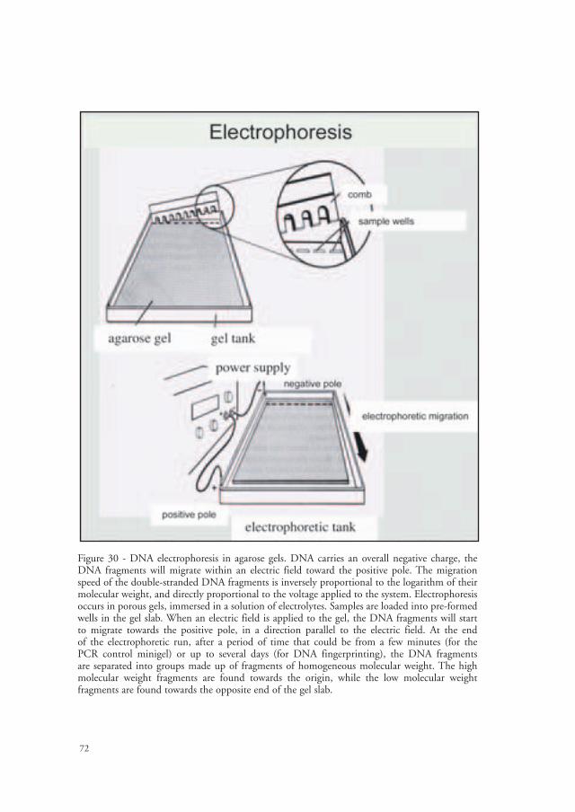
72

Figure 30 - DNA electrophoresis in agarose gels. DNA carries an overall negative charge, the DNA fragments will migrate within an electric field toward the positive pole. The migration speed of the double-stranded DNA fragments is inversely proportional to the logarithm of their molecular weight, and directly proportional to the voltage applied to the system. Electrophoresis occurs in porous gels, immersed in a solution of electrolytes. Samples are loaded into pre-formed wells in the gel slab. When an electric field is applied to the gel, the DNA fragments will start to migrate towards the positive pole, in a direction parallel to the electric field. At the end of the electrophoretic run, after a period of time that could be from a few minutes (for the PCR control minigel) or up to several days (for DNA fingerprinting), the DNA fragments are separated into groups made up of fragments of homogeneous molecular weight. The high molecular weight fragments are found towards the origin, while the low molecular weight fragments are found towards the opposite end of the gel slab.

73

The migration speed of the double-stranded DNA fragments is inversely proportional to the logarithm of their molecular weight, and directly proportional to the voltage applied to the system. Electrophoresis occurs in porous agarose or acrylamide gel, immersed in a solution of electrolytes. Each sample is loaded into its own pre-formed wells in the gel slab. When an electric field is applied to the gel, the DNA fragments will start to migrate towards the positive pole, in a direction parallel to the electric field. At the end of the electrophoresis run, after a period of time that could be for a few minutes (for the PCR control minigel) or up to several days (for DNA fingerprinting), the DNA fragments are separated into groups made up of fragments of homogeneous molecular weight. The high molecular weight fragments are found towards the origin, while the low molecular weight fragments are found towards the opposite end of the gel slab. The concentration of agarose or acrylamide influences the migration speed, but above all the focalisation and the resolution of the fragments in relation to their molecular weight. Gel with a concentration of 1% - 2% agarose is usually used. The gel is soaked in ethidium bromide dye (EtBr) that binds exclusively to double-stranded DNA and makes it temporarily visible under ultraviolet light. DNA appears as a fluorescent compact band if the sample is not degraded or as a smear if the sample is degraded (Fig. 27). Highly degraded DNA may not be visible in agarose minigel. It is important to note that EtBr highlights all the DNA present in the minigel, that is, the DNA of the sample as well as any possible contaminant DNA. Electrophoresis through agarose gel is used to control DNA extraction, digestion and amplification, as well as for RFLP analysis. Microsatellite and nucleotide sequence analysis is carried out through acrylamide gel.

Southern blotting

Agarose gel is delicate and creates problems in carrying out hybridisation, washes and autoradiography. Moreover, DNA fragments tend to spread rapidly in agarose when, at the end of electrophoresis, the electric current is cut off. These problems are resolved through a technique known as Southern blotting (Southern 1975), which consists in transferring the DNA from agarose gel to a nylon membrane. The procedure for Southern blotting is illustrated in figure 31. Double-stranded DNA is denatured by immersing the agarose gel in an alkaline solution, then the gel is neutralised in a high saline concentration

74

solution, to maintain the denatured DNA. A piece of nylon membrane is placed on top of the gel and layers of absorbent material on top of that. The absorbent material draws up the liquid from the gel and the DNA fragments along with it. The membranes are strong, chemically resistant, and have a positive charge, which facilitates the absorption and contact with DNA fragments that have a negative charge. When blotting is completed, the DNA fragments adhere permanently to the membrane, as they are exposed to UV rays for a few minutes in a transluminator.

Figure 31 - Southern blotting consists in transferring the DNA from agarose gel to a nylon mem-brane. Double-stranded DNA is denatured by immersing the agarose gel in an alkaline solution, then the gel is neutralised in a high saline concentration solution, to maintain the denatured DNA. A piece of nylon membrane is placed on top of the gel and layers of absorbent material on top of that. The absorbent material draws up the liquid from the gel and the DNA fragments along with it. The membranes are strong, chemically resistant, and have a positive charge, which facilitates the absorption and contact with DNA fragments that have a negative charge. When blotting is completed, the DNA fragments adhere permanently to the membrane, as they are exposed to UV rays for a few minutes in a transluminator.

75

Molecular hybridisation

Once Southern blotting is completed the membrane, containing the fixed DNA fragments is used for hybridisation with oligonuclotide probes (Fig. 32). These probes are designed to match sequences in the genome that are well-characterised and highly polymorphic. DNA strands that match will bind into a double-stranded form (annealing) and any probe fragments that have not bound specifically are washed away so as not to interfere with the signal. This process is called hybridisation. The labelled fragments signal where they have hybridised and this signal is recorded on a sheet of X-ray film. The pattern recorded on the exposed film is

Figure 32 - Once Southern blotting is completed the membrane, containing the fixed DNA fragments is used for hybridisation with oligonucleodite probes. These probes are designed to match sequences in the genome that are well-characterised and highly polymorphic. DNA strands that match will bind into a double-stranded form (annealing) and any probe fragments that have not bound specifically are washed away so as not to interfere with the signal. This process is called hybridisation. The labelled fragments signal where they have hybridised and this signal is recorded on a sheet of X-ray film.

76

called an autoradiogram. Different hybridisation protocols are calibrated to optimise the signal in relation to the probes that are utilised. It is necessary to standardise hybridisation conditions for every type of probe. The following protocol is used at the INFS Laboratory of Genetics.

INFS protocol for DNA fingerprinting analysis

(1) Phenol-chloroform DNA extraction of blood samples:

Blood samples are often used for multi-locus DNA fingerprinting analysis. DNA is extracted with the phenol-chloroform method, following the protocol described above.

(2) Spectrophotometric DNA quantification:

Extracted DNA is run through agarose minigel, to verify the total DNA that has been obtained. Then the concentration of DNA is controlled through spectrophotometry analysis. It is necessary to digest approximately 10 - 12 µg (1 µg = 1 γ) of DNA per sample to obtain good quality autoradiograms. Spectrophotometric concentrations of extracted DNA must be about 50 (minimum) - 300 (maximum) µg/ml.

(3) Digestion with restriction enzymes:

To assure that digestion is complete, two consecutive digestions are carried out for each sample. The first digestion takes place at 37°C overnight, in a total volume of 200 µl, that includes:- no more than 175 µl of DNA in solution, corresponding to approx.

10 - 12 γ of DNA;- 3 - 5 µl of restriction enzyme;- 20 µl of digestion buffer;- addition of sterile ddH2O up to the necessary volume.

The second digestion takes place at 37°C for about 4 - 5 hours, adding 100 µl of digestion solution for each sample (1 µl of restriction enzyme; 10 µl of digestion buffer, 89 µl of ddH2O).

At the end of the second digestion a control should be made through minigel that the DNA was digested well, that is, that no high molecular weight fragment are present, and that it is visualised as a homogeneous band. Digestion control is done by placing 5 µl of digested DNA + 5 µl of EtBr that runs through agarose minigel via electrophoresis at 150 - 200 volts for a few minutes. Digested DNA can be preserved in freezer at -20°C.

77

(4) Precipitation and re-suspension of digested DNA:

Approx. 30 µl of 3M sodium acetate (NaAc), that is about 1/10 of the volume of digested DNA solution, are added to digested DNA. Then the following procedures are done:- add about 2.2 volumes of ethanol 100% (about 700 µl), better if cold; - mix delicately and place the solution at - 20°C for 30 min;- centrifuge at 17,000 rpm for 30 min at 4°C; in this way DNA forms a

pellet;- eliminate the supernatant without detaching the pellet;- add 1 ml of ethanol at 70%;- centrifuge at 17,000 rpm for 15 min at 4°C;- dry samples at room temperature;- re-suspend the DNA pellet in 20 - 25 µl of TE.

(5) Electrophoresis through agarose gel:

Agarose gel is prepared at a concentration of 1% or 0.8% in TBE buffer; 5 µl of bromophenol blue + glycerine at 30% is added for every sample (the blue forms a clearly visible line that migrates faster than any DNA fragment and is necessary to control electrophoresis; glycerine is needed to thicken the samples and facilitate their loading into the wells in the agarose gel).

Loading the samples on the gel. The order in which the samples are loaded on the gel is very important, because the evaluation of DNA fingerprinting is done by directly comparing the electrophoretic migration speed of the various DNA fragments among the different samples. When parental testing is carried out, the following loading procedure is used:1 = standard molecular weight (lambda DNA digested with Hind III, or

other molecular weights)2 = control sample3 = putative father4 = offspring 15 = offspring 26 = putative mother7 = molecular weight

The electrophoresis run is carried out at 25 - 30 volts for 2 - 3 days. Buffer TBE 1X in the buffer reservoirs are completely substituted every 24 hours.

(6) Southern blotting:

Once electrophoresis is terminated, the DNA fragments on the agarose

78

gel are denatured through a series of washes. The first wash is done with a depurination solution (27.33 ml/lt HCl) for 15 min on a shaker. Depurination breaks the bonds between one purine and the next, and aids the blotting of DNA fragments from the gel to the membrane. The gel is washed in ddH2O. Then the gel is immersed in denaturant solution (0.5 M NaOH = 20 gr/lt; 1.5 M NaCl = 88 gr/lt) twice for 15 min. The gel is washed again in ddH2O. Then the gel is immersed in neutralising solution (0.5 M Tris = 60.55 gr/lt; 1.5 M NaCl = 88 gr/lt; EDTA.Na2 = 0.4 gr/lt; pH 7.2) twice for 15 min.

Blotting, that is, the transfer of DNA fragments from agarose gel to a nylon membrane, is carried out in a blotting solution (20x SSC: 3 M NaCl = 175.33 gr/lt; 0.5 M Na tribasic citrate dihydrate 88.23 gr/lt; pH 7.0 - 7.5. Then the necessary equipment for Southern blotting is prepared (Fig. 31). Blotting takes place overnight.

(7) Pre-hybridisation and hybridisation:

Once blotting has terminated, the membrane is prepared for hybridisation with a labelled probe. The membrane is washed in 5x SSC (50 ml in 200 ml H2O), then the DNA is fixed via exposure to UV for three min on the transilluminator. The membrane is then washed in 1x SSC (10 ml in 200 ml of ddH2O) at 50°C in rotation.- Pre-hybridisation. The membrane is pre-hybridised once at 50°C in

rotation for 20 min, in 50 ml of pre-hybridisation solution (49.5 ml of 0.5 M Na2HPO4; pH 7.2 = 71 gr/lt; 0.5 ml SDS 10% = 100 gr/lt).

- Hybridisation. The membrane is pre-hybridised once for 20 min at 50°C in rotation, in 20 ml of hybridisation solution, prepared with:

18 ml of pre-hybridisation solution 2 ml of block solution (10 gr of casein in 100 ml of washing

solution #2), to which 10 µl of labelled probe is added.At the end of hybridisation the membrane is washed repeatedly:

- 1st wash: twice for 10 min at 50°C, in rotation, with 100 ml of washing solution #1 each time:

166 ml ddH2O32 ml 0.5 M Na2HPO4; pH 7.2 (0.71 gr/lt)2 ml SDS 10%

- 2nd wash: twice for 10 min at room temperature, on a shaker, with 200 ml of washing solution #2 each time:

100 ml of 4x washing solution #2 (maleic acid: 55.2 gr/lt; NaCl: 34.8 gr/lt; pH 7.5 with NaOH) in 400 ml of ddH2O.

79

(8) Incubation with detector. Exposure and development of autoradiography film:

The INFS DNA fingerprinting protocol uses two Jeffreys multi-locus probes. The first, the 33.6 probe, has an incubation period of about 18 hours in man and primates, and about 2 - 3 days in other mammals and in birds. The second, 33.15 probe, has an incubation period of 3 hours in man and primates and about 1 day in other mammals and birds. These two probes are protected by a patent (UK Patent No. 2166445) and are manufactured by Cellmark Diagnostic (PO Box 265, Abington, Oxon OX14 IYX, UK; cellmark@orchidbio.co.uk.). The Cellmark probes are labelled with the alkaline phosphatase enzyme and manufactured as “NICETM non-isotopic probe system”, a product which eliminates the use of radioactive isotopes and the need of labelling probes in the laboratory as well as guaranteeing high quality results. By applying reagents Lumi-PhosTM or the more recent CDP-StarTM to the membrane, it is possible to visualise the response of alkaline phosphatase. These reagents activate the alkaline phosphatase enzyme that starts the chemioluminescent reaction. Light is emitted for at least 5 days, and allows X-rays photographic film to be exposed rapidly. Alternatively, it is possible to clone, purify and label the probes in one’s own laboratory. Oligonucleotide probes can be labelled with radioactive isotopes, for example, binding phosphorous atoms to a nucleotide (for example: a-32PdCTP), or incorporating, for example, alkaline phosphatase in non-radioactive labelled probes.

Once the washing phase is completed, the membrane is covered with Lumi-PhosTM or CDP-StarTM, sealed in a plastic bag and placed in a container for autoradiography. At this point one enters the dark room and places an autoradiographic film in contact with the membrane. The autoradiographic container is then closed and the film is exposed for the necessary time. This autoradiographic film is then processed. The developed film is then washed with water and left to dry.

If necessary, the membrane can be re-hybridised. The probes, fixed to the complementary DNA fragments, can be washed with SDS 0.1% (0.5 ml SDS; 49.5 ml H2O) for 15 min at 80°C in rotation, and then with 1x SSC (10 ml in 200 ml H2O) at 50°C in rotation. At this point the membrane can be re-hybridised, repeating the procedures for pre-hybridisation, hybridisation, washing, etc., using the same probe or another. Seven to nine working days are necessary to complete all the procedures in the INFS protocol for multi-locus DNA fingerprinting.

80

Structure of multi-locus probes used in forensic genetics

The probes used in forensic genetics are made up from single or double stranded DNA or RNA that contain the complementary sequences of the repeated sequences of loci used to obtain DNA fingerprinting. These genetic markers have been chosen because they are very polymorphic, and because they can be typed in almost all vertebrate species, hybridising the multi-locus probes to the DNA of samples at low stringency conditions. Minisatellites are regions of genomic DNA made up of short tandemly repeated sequences. Polymorphism derives from the differences in molecular weights among different alleles. The difference in molecular weight depends on the different number of repeats that make up the alleles. Every minisatellite locus has numerous alleles in each population, and therefore the values of heterozygous individuals are very high. The variability among alleles probably derives from asymmetric crossing-over or from DNA slippage during meiosis. The variability in allele lengths at minisatellite loci can be detected by digesting the DNA with restriction enzymes, that cut the minisatellite at the flanking region, and not within it. Numerous minisatellite loci have been identified that map within or in proximity of genes, such as the gene for human insulin, several genes for the globins and others for oncogenes. The first minisatellite was discovered and characterised by Alec Jeffreys and his collaborators in 1985. This minisatellite, identified in the first intron of the human mioglobin gene (Fig. 14) is made up of four repeated of a sequence 33 nucleotides long. The minisatellite is flanked by non-repeat sequences that contain two restriction sites for the endonuclease HinfI. Digestion with HinfI permits a segment of the intron that is 169 nucleotides long, containing all the minisatellite, to be isolated. Digesting this segment with other endonucleases that have restriction sites within the repeat, it was possible to isolate and clone the monomer 33 nucleotides long. This sequence, the so-called “core” sequence, was used to create the multi-locus 33.7 probe. By cloning minisatellite loci identified through probe 33.7, it was possible to identify new loci, each containing from 3 to 29 copies of a repeat identical or similar to the core sequence of the minisatellite contained in the first intron of the human mioglobin gene. Each of these loci map into a unique region in the human genome. Multi-locus probe 33.15 and 33.6 were obtained from two of these loci. These probes are hypervariable, that is, they contain multiple alleles in human populations and in many other vertebrates species.

Jeffrey’s multi-locus probe 33.15 is made up of 32 nucleotides that are subdivided into two repeated sequences of 16 nucleotides:

81

MLP 33.15 = (TCTCCACCCGTCCACC)2

This probe is complementary to the repeat AGAGGT-GGGCAGGTGG.- Probe 33.6 is made up of 37 nucleotides that include three repeated

sequences of 11 nucleotides each:

MLP 33.6 = (TCCCGACCTCC)3

This probe is complementary to the repeat AGGGCTGGAGG.The underlined nucleotides correspond to the “core” sequence:

GGGCAGGAxG, that is present, though not perfectly conserved, in all the repeats of each minisatellite detected by Jeffrey’s probes.

Every autoradiographic or fluorographic film identifies individual profiles that are usually composed of 10 to 30 DNA fragments, each representing an allele. Though Jeffrey’s probes have been developed and principally utilised for human DNA analysis, they are also useful for DNA fingerprinting analysis in other animal species. Good quality DNA fingerprinting has been obtained in many vertebrate species including canines, felines, birds, and fish. Other probes have been cloned that can be used not only in human forensic genetics but also in plant and animal species, such as, the α-globulin minisatellite and the repeat contained in the bacteriophage M13. Oligonucleotide probes that have been synthesised chemically are also used.

The mutation rate of minisatellites identified by Jeffreys has been calculated as 1 x 10-4 new alleles per gamete per generation, which means that there is an allelic mutation every 10 000 gametes. This mutation rate is at least one order more than the rate of symmetrical recombination, and is several orders than the rate of nucleotide substitution at selectively neutral loci.

Interpretation of DNA fingerprinting

Autoradiograph analysis (autorad) is complicated because of the great number of fragments (alleles) that are present in individual profiles and because of the great inter-individual variability of DNA fingerprinting. The problem lies in identifying which fragments of every profile are “identical” and which are “different” from one individual to another. Determining the correspondence between individual fragments can be done visualy, or through a computerised systems. In any case, it is necessary to consider the procedural factors that can create approximations in the identification of DNA fingerprinting profiles, such as width and intensity of fragments,

82

quality of the electrophoresis resolution, variations of electrophoresis mobility within a gel, possible deformations of electrophoresis migration to different areas of the gel. These errors in the various phases of analysis could create a situation in which two identical fragments are visualised as different, or vice versa, that two fragments of different molecular weight are visualised as identical. Hence it is necessary to establish the identification criteria for mobility and to assign the molecular weight of fragments, that take account of these errors. Usually, two fragments are identified as identical if they have a molecular weight that is determined within 3 units of the standard deviation in any migration direction. In well-calibrated electrophoresis systems, every fragment has a standard deviation that corresponds to about 0.6% of its molecular weight. For example, the definition of a fragment of 4000 nucleotides can vary 25 nucleotides x 6, and therefore fragments of 4000 +/- 150 nucleotides are assigned to the same allele and are considered identical.

Apart from technical problems, deriving from the quality of the laboratory procedures and from the identification of fragments in DNA fingerprinting, MLP systems present other problems. Normally, the variability of MLP systems is so high that it is extremely improbable, but not impossible, that two individuals have the same DNA fingerprinting. It is difficult to estimate what the probability of identity (PID) is between two individuals chosen randomly in a reference population, because the genetics of fragments (that is, the number of loci that were identified, the number of alleles at every locus, the number of homozygous or heterozygous loci in the analysed sample, etc.) that make up a DNA fingerprinting is unknown. It is not simple to estimate the linkage relationship between the “alleles” of a MLP system. If a subgroup of MLP “alleles” are linked, then they were inherited as a single group from the parents, hence the power of identification can be much less than it seems if all the system were composed of non-linked “alleles”.

SLP probes locate specific, single minisatellite loci. Therefore every individual can be characterised by one (homozygous) or two (heterozygous) DNA fragments at each locus, and not by a system of multiple bands as in MLP systems. These VNTR loci have many alleles and present very high heterozygosity values. The multi-locus individual genotype is determined by separately analysing several loci (usually 4 - 6) and cumulating the data, that is, forming multi-locus genotypes that correspond to DNA fingerprinting in MLP systems. VNTR loci have the advantage of being well identifiable, in that they have a maximum of two alleles per individual, though many alleles in the population.

83

DNA amplification

Restriction fragment analysis through Southern blotting requires 1 to 10 gamma of total, high molecular weight DNA. However, biological samples available for forensic genetic analysis often contain little DNA, which is sometimes degraded. Therefore DNA amplification becomes a necessary procedures in obtaining sufficient sample quantity for molecular analyses. DNA sequences made up of a few dozen or few thousand nucleotides can be amplified effectively using PCR (polymerase chain reaction). PCR allows several micrograms of DNA in a test tube to be synthesised starting from a few picograms of the sample. In theory, it is possible to use a single molecule of target DNA (that is, the gene or the DNA sequence that must be analysed and which therefore must be amplified). Sequences present in a single copy in DNA samples can be amplified up to 10 million times in a few hours. Amplified DNA consists of multiple copies of the target sequence, and is sufficiently pure to be directly sequenced or analysed through other molecular techniques. PCR (Fig. 33) occurs by reconstructing the chemical conditions necessary to obtain DNA synthesis in vitro. First, it is necessary to identify the gene or DNA sequence that one wishes to amplify (for example, the control-region of mitochondrial DNA, or a microsatellite locus). The sequence to amplify is flanked on either side by sequences that must be at least partially known. In fact, to start off PCR, it is necessary to synthesise a pair of oligonucleotides “primers” that are at least partially complementary to the flanking sequences. The oligonucleotides used as primers are chemically synthesised, and are usually produced by specialised, commercial laboratories that use automated instruments. It is necessary to supply the commercial laboratory with the primer sequences, which must be carefully determined. The primers bind to the flanking complementary sequences, which allows the duplication process of the target sequence to start. Every PCR consists of a cycle, repeated many times, made up of the following steps: denaturation of the DNA sample; binding of the primers to the flanking sequences; extension of the primers through the enzymatic action of a DNA polymerase, which ends in the complete replication of both strands of the target sequence. PCR occurs in a test tube that contains: the DNA sample, the two primers, the DNA polymerase enzyme, a certain quantity of free nucleotides, all this in a buffer solution that optimises DNA synthesis. Every test tube for PCR is placed in a thermal cycler that carries out a prefixed thermal cycle with great precision, shifting rapidly from the denaturation temperature (above 90°C, for a few

84

seconds) to primer binding temperatures (which vary from 40 to 55°C, for a few seconds) to extension temperature (72°C for several seconds), only to start again with the denaturation temperature, and so on, from 20 to 40 times. The thermal cyclers are designed to accommodate test tubes or 96 well “microtiter” plates, in which the PCR reagents are mixed. As the thermal cycle can be carried out rapidly, it is possible to amplify up to 96 samples in one to two hours. Firstly, the DNA sample is denatured thermally, that is, raising the reaction temperature up to 90 - 95°C. When the DNA is denatured, that is, when the double helix is completely dissociated in the two single strands, each of the primers attach themselves (annealing) to the complementary sequence that flanks the sequence of the target DNA. The annealing temperature depends on the length of the primers and their sequence. This usually varies from 40 to 55°C,

Figure 33 - The polymerase chain reaction (PCR).

85

and must be determined and checked carefully to make sure that the primers do not anneal to themselves or to non-target sequences, and consequently produces aspecific amplifications. When annealing is complete, a thermoresistant DNA polymerase (Taq polymerase) intervenes, which starts the duplication of the target DNA starting from the priming sites. The polymerisation reaction occurs in a buffer solution that maintains the correct pH level, an optimum concentration of Mg++ ions, and which contains free nucleotides in an active form (dATP, dCTP, dGTP and dTTP) that can be incorporated during DNA synthesis. Synthesis occurs via extension of both primers. The Taq polymerase catalyses the extension of the primer and produces two new DNA strands, which are complementary to the target strands. Primer extension occurs at an optimum temperature for DNA synthesis, usually at 72°C. Therefore PCR proceeds thanks to a cycle of three temperatures: the DNA denaturation temperature, the annealing temperature of the primers to the target sequence (40°C - 55°C), the extension of the primers temperature (72°C). The time necessary for the PCR reaction at these three temperatures can vary, but isusually quite short, that is, a few seconds each. By the end of the first cycle, every form of the target sequence present in the sample is replicated once, at this point the cycle is repeated a second time, the thermal cycle of the PCR is repeated many times (usually 20 to 40 times), and so produce an exponential replication of the target sequence. In fact, with every successive cycle the synthesised DNA is doubled (Fig. 34).

PCR efficiency depends on the capacity to faithfully amplify the target DNA, and only the target DNA. If the sequence of the target DNA is amplified by inserting wrong nucleotides, then the PCR would generate false “mutations”, which in reality are not present in the sample. If the primers anneal not only to the target sequence but also to other sequences present in the DNA samples then the PCR would amplify “aspecific” sequences which would made the analysis and interpretation of the results problematic and even impossible. Efficiency and specification of PCR can be checked and improved by optimising the experiment conditions in each case. It is very important to use top quality Taq polymerase. These polymerases are also stable at high temperatures, therefore are not degraded when subjected to repeated cycles of denaturation. It is also very important to identify extremely specific primers, which are strictly complementary to the flanking sequences of the targets. The use of specific primers avoids amplification of contaminating DNA. One of the fundamental advantages of PCR is

86

that it allows very small quantities of the target DNA to be amplified. Nonetheless, PCR in the presence of small quantities of target DNA is exposed to contamination with exogenous DNA. Contamination may occur on biological samples before the DNA is extracted in the laboratory, or in the laboratory during DNA extraction and amplification procedures. It is necessary to equip the laboratory and apply stringent quality controls to avoid contamination, or to locate it once it has occurred. PCR efficiency can be limited by the presence of Taq inhibitors that are present in the samples. It is possible set up PCR to amplify more than one locus at the same time (PCR multiplex).

Random Amplified Polymorphic DNA (RAPD )

Other PCR techniques have been developed recently that can be used in forensic genetics. The RAPD technique (Random Amplified

Figure 34 – Exponential amplification of the target DNA during a PCR.

87

Polymorphic DNA) allows random amplification of DNA genome fragments through the use of random sequencing primers. The sequences and the choice of primers are random in the sense that the information concerning the presence of possible complementary annealing sites in the genome of analysed samples is unknown. The primers are about 10 nucleotides long and have random sequences. The RAPD method is a PCR that uses only one primer and a low annealing temperature. In fact, the RAPD primers are not very specific and only attach to the complementary sequences at low annealing temperatures. When two RAPD primers identify two complementary sequences within about 2000 nucleotides of each other, then PCR amplifies the double-stranded DNA fragments, which correspond to the DNA region included among the annealing sites of the two primers. Amplified DNA fragments are then separated in agarose gel at 4% and detected using EtBr, or in an acrylamide gel at 3 - 5%, stained with silver staining. The RAPD method usually works better in plant than in animal DNAs. Every single RAPD primer can generate a large number of fragments, which are often hypervariable and polymorphic. However this method does have some limitations. RAPD genotypes do not usually correspond to DNA fingerprinting, because the single individuals are not distinguishable. The number and the quality of the amplified fragments vary according to the quantity and quality of the DNA sample. The RAPD method is very sensitive to slight variations of a series of experimental factors which include DNA extraction, PCR procedures and electrophoresis. Interpretation of RAPD results may require subjective choices. This technique amplifies the DNA sample as well as the contaminant DNA. From a genetic point of view, RAPD fragments cannot, by definition, be traced back to specific loci, therefore it is either impossible or very difficult to identify possible alleles. Another complication derives from the relation of dominance among RAPD fragments: a fragment that amplifies on a chromosome is dominant on the fragment that it does not amplify and, therefore heterozygotes cannot be identified. The RAPD technique can be used for molecular sexing.

Amplified Fragment Length Polymorphism (AFLP)

In the AFLP (Amplified Fragment Lenght Polymorphism) method the DNA is cut by two restriction enzimes, usually EcoRI e MseI. Then the restriction enzimes are bound to oligonucleotides that serves as primers annealing sites (adapters). Two specific adapters are bound to the two

88

fragment estremities (5', 3') by ligase enzime. The fragment with the adapters are reamplified using pairs of primers that are complementary to the adapters. At the latters, at the 3' extremity, are added one to three random nucleotides (selective nucleotide). The number of primer combinations that can be used to perform selectives PCRs is very high, and they have to be optimized to obtain repeatable amplification of 50-100 fragments. The fragments are separate by sequencing gel electrophoresis that can separate fragments in a size range of 400-500 nucleotides. The AFLP fragments can be visualised by radioactively labelled primers (manual electrophoresis), or by fluorescent labelled primers (automated electrophoresis). Now forensic genetic AFLP application is limited to cases of species and hybrid identifications starting from DNA extracted from tissue samples or from specimens from animals derived of unknown origin. AFLP techniques can be used for molecular sexing.

DNA sequencing

Methods used today for DNA sequencing were developed by Maxam and Gilbert, and Sanger and collaborators in 1977. These methods use two different approaches to determine DNA sequences. Most DNA sequencing today is performed using automated platforms that are based on the Sanger method. The DNA fragment that needs to be sequenced is denatured. An oligonucleotide primer complementary to one of the two DNA strands to be sequenced is used to start DNA duplication. In the synthesis reaction four deoxynucleotides (dATP, dGTP, dCTP, dTTP) are added as well as four dideoxynucleotides (ddATP, ddGTP, ddCTP, ddTTP). The dideoxynucleotides are modified base analogues of deoxynucleotides. When the dideoxynucleotides are incorporated in the DNA, the extension is interrupted, generating fragments that terminate with one of the four dideoxynucleotides. The fragments are then separated by electrophoresis through acrylamide gel or in automated capillary sequencers (Fig. 35).

Sequencing reactions are PCR reactions carried out using only one primer, that is, the sequence primer, and by adding predetermined quantities of dideoxynucleotides to the reaction. The choice of sequence primer determines the sequence that is obtained, which corresponds to approximately 300 - 800 nucleotides that are in 3’ position compared to the primer (DNA duplication and therefore extension of the primer occurs at 5’ -> 3’). In PCR sequencing only one primer is used and

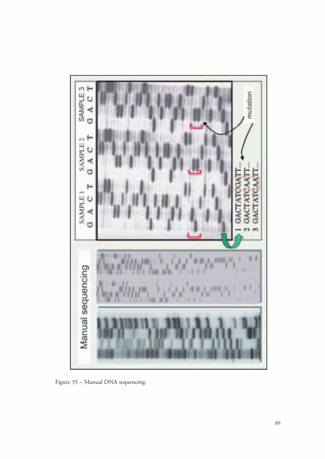
89

Figure 35 – Manual DNA sequencing.

90

the amplifications of the product will be linear and not logarithmic, as happens in reactions of PCR amplification. The number of cycles of PCR sequencing depends on the quantity of DNA used, but it does not usually present serious problems. Before electrophoresis in an automated sequencer, the product of PCR sequencing must be purified to remove the primer or the unused terminators. A simple precipitation of DNA through ethanol is usually sufficient to obtain good purification. DNA sequences can be preserved lyophilised or frozen at -20°C for several months. Before electrophoresis, samples are re-suspended in sequencing buffer, that contains formammide, a denaturing substance. DNA solution is denatured at a high temperature and immediately loaded into the sequencer.

Automated sequencing exploits fluorescent-based detection of sequencing products. The automated sequencers are used not only to sequence DNA, but also to visualise and analyse microsatellites, fragments generated via RAPD and AFLP techniques, VNTR loci (minisatellites) and single-stranded conformational polymorphisms (SSCP). Automated sequences have a series of multiple capillary columns (usually from 16 to 96) and are perfectly adapted to automatically load the reactions to analyse, directly from the microtiter plates. The capillary sequencers do not use radioactive markers, or other toxic substances like acrylamide, therefore eliminate this health risk in the work place. Fluorescent markers systems use molecules called “fluorescent dyes” that are more sensitive than marking systems that use radioisotopes and are much more sensitive than silver staining systems. Fluorescent dyes are incorporated in the DNA during PCR amplification or sequencing, utilising primers labelled beforehand with a fluorescent dye, or incorporating a labelled nucleotide in the DNA. The labelled DNA is detected during electrophoresis performed by the automated sequencer: when the labelled DNA fragment passes a pre-set location, the fluorescent dye is picked up by a laser, and the emission of fluorescence is detected and measured. There are different types of fluorescent dyes that emit different wave lengths that are read as different colours (Fig. 36). Therefore it is possible to label DNA fragments with different colours that are detected and analysed at the same time. In this way it is possible to mark the four nucleotides with four different colours and analyse the results of the sequence reactions in a single capillary column. It is possible to mark the primers for microsatellite amplification with different colours and analyse many microsatellites of different molecular weights in a single capillary column, at the same time. A molecular weight standard is added to every capillary, labelled

91

with a colour that is not used to mark the primers or the nucleotides. This permits precise regulation of molecular weights and fragments analysed within every capillary.

Acrylamide gel (usually a denaturing gel at 6% concentration) is used in first generation sequencers. A thin layer of gel, 0.2 - 0.4 mm thick, is an essential condition needed in obtaining good results from electrophoresis sequencing. It is also extremely important that the glass plates used to prepare the template for the gel are absolutely clean, and that all the products, including water, used to prepare the gel are as pure as possible. Impurities present in the glass plates and in the gel can produce background colours, which can mask the signals of the fluorescent tags and therefore make the reading of sequences impossible. The second generation capillary sequencers do not require the gel preparation. In fact, the sequencer automatically injects the gel in the capillaries. In this way all the problems regarding the manual sequencing method are eliminated including impurities. Every set of capillaries must be substituted after approximately 100 - 200 electrophoreses. Electrophoresis is programmed through particular computer software that activates and controls all the operations performed by the automated sequencer. When electrophoresis of the samples is completed, the sequencer creates files in the computer that contain all the necessary information to accurately determine the sequences.

Figure 36 - Automated DNA sequencing: the electropherogram.

92

During each electrophoresis, the computer reconstructs one or more image files from real-time laser detection of the colour-specific fragments. Once the electrophoresis has terminated, these files are permanently saved (Fig. 37). Sequencing results are saved in the form of “electropherograms” (Fig. 36) when a fluorescent dye picked up by a laser produces a luminous emission that is registered as a peak. The height of the peak indicates the intensity of the emission and the colour indicates the colour of the fluorescent dye. As every colour is associated with a specific termination reaction, the sequence of coloured peaks in the electropherogram corresponds exactly to the DNA sequence. The electropherogram file contains the DNA sequence written with the four letters that correspond to the four nucleotides. The positions of the nucleotides are numbered in groups of ten from the beginning of the sequence. In the case that a particular peak cannot be univocally

Figure 37 - Automated DNA sequencing: image of the sequencing procedure. During each electrophoresis, the computer reconstructs one or more image files from real-time laser detection of the colour-specific fragments. Once the electrophoresis has terminated, these files are permanently saved.

93

determined, the software signals the presence of an ambiguity (sequence not determined = N). The sequence furnished by the electropherogram can be adjusted through software programme that allows one to manually assign any possible ambiguous nucleotides. Portions of the sequence that have not been determined accurately can be eliminated. This usually occurs in the first and final part of every electropherogram. The correct sequences are then transcribed in written files. The written files are aligned with other reference sequences that are included in the database and analysed.

PCR products are usually sequenced directly. To obtain good sequences, it is important that the DNA is purified and does not contain contaminants that inhibit the PCR (for example residue of organic products such as phenol and chloroform that inactivate the Taq polymerase). PCR products must be specific and must not contain aspecific fragments that produce multiple or illegible sequences. If PCR products contain contaminants or aspecific fragments they must be purified by electrophoresis through agarose minigel. The specific fragment is recovered, by cutting the portion of gel that contains it. The fragment is then separated from the agarose by electro-elution, or by digestion from the agarose with an agarose enzyme. Before sequencing, the PCR products must be purified, that is, it is necessary to eliminate the nucleotides and the PCR primer that were not used and that could interfere with PCR sequencing.

It may be necessary to clone the amplified fragments that contain two alleles (heterozygous fragments) and sequence the clone to determine the differences between the two alleles. The presence of dimers among PCR primers can produce sequencing artefacts, above all if one of the PCR primers is used as a sequencing primer. To eliminate or reduce these artefacts it is possible to use “hot start” PCR techniques, that is, PCR that begins at high temperatures. High temperatures impede the formation of dimers and make the interaction between the primer and the target DNA more specific. The hot start PCR is carried out using modified Taq polymerases that are activated only at high temperatures, that is, when weak interactions between dimers and aspecific interactions are no longer possible.

Mitochondrial DNA structure and sequencing

The mitochondrial genome, the mitochondrial DNA, is a simple, haploid molecule that apparently does nor recombine (though in some

94

cases may recombine). The mtDNA is a double-stranded circular molecule, generally made up of several thousand nucleotides. It is only inherited from the mother (though exceptions have been documented). Every mtDNA sequence, defined as an “haplotype”, is transmitted intact from one generation to the next, and therefore can be used to reconstruct the genealogy of populations and to identify individuals that belong to different populations, subspecies and species. Mitochondrial genes evolve more rapidly, on average, than nuclear genes and therefore rapidly accumulate genetic differences among populations of conspecific organisms. Mitochondrial DNA analysis is very useful in identifying populations that evolve independently, taxonomically distinct population groups, cases of hybridisation and gene flow.

The organisation of mtDNA is quite stable. All metazoan mitochondrial DNA contain genes that codify for enzymatic proteins, other genes that codify for two ribosomal RNA, and some that codify for RNA transfer (Fig. 11). Moreover, the mitochondrial genomes possess at least one control-region, that does not codify for proteins nor for RNA, but has the role of controlling replication and transcription of the entire mitochondrial genome. The order of the genes in mtDNA is quite conserved. But numerous rearrangements exist. Mitochondrial DNA evolves 5 - 10 times more rapidly than nuclear genes. In particular, the control-region evolves much more quickly than nuclear sequences. The control-region contains several short hypervariable sequences that evolve very rapidly and that are extremely useful in population genetics and in forensic science. Normally, mitochondrial sequences are analysed by nucleotide sequencing.

Amplification and analysis of microsatellites

Repeated sequences of microsatellites are flanked by unique sequences. Hence it is possible to design PCR primers that selectively amplify microsatellite loci. Genotype analysis is done to identify the molecular weight of the alleles present at each locus via electrophoresis. As in the case of VNTR loci, individual genotypes are determined by separately analysing a certain number of microsatellites (usually 5 - 6), and accumulating the data, that forms multi-locus genotypes that correspond to DNA fingerprinting of MLP and SLP systems. Microsatellites have the advantage of being genetically well identifiable, having a maximum of two alleles per individual, but many alleles in the population. Microsatellites have a further advantage over VNTR loci: they can be

95

amplified through PCR and therefore typed from any kind of biological sample, independently from the concentration of DNA or its state of degradation.

Microsatellites present in the genome of a species are individualised by cloning techniques, that allow DNA sequences to be isolated which contain the microsatellite as well as the flanking sequences. The two flanking sequences and the structure of the microsatellite can be identified by nucleotide sequencing. Analysis of the flanking sequences consists in designing the PCR primers. The variability expressed by each new microsatellite locus must be characterised in a sample survey of individuals taken from the reference population. In fact not all microsatellite loci are polymorphic. Microsatellite analysis is done by separating the alleles by electrophoresis in a denaturing gel (sequencing gel), which clearly separates the two alleles present at the heterozygous loci (Fig. 15). Electrophoresis must be carried out with extreme technical precision, as the difference in molecular weight of the alleles depends frequently on two (in dinucleotide microsatellites), four or six nucleotides. Not all microsatellite alleles are made up of a perfect repeat, and sometimes, the difference between the two alleles is due to a single nucleotide. Therefore the electrophoresis system must be capable of separating and identifying fragments (alleles) that differ by only one nucleotide, exactly as in sequencing gel. In forensic genetics it is advisable to analyse the microsatellites using automated sequencers on acrylamide gel or in capillary systems.

Analysis of microsatellites in automated sequencers

In automated sequencers, it is possible to analyse several microsatellite loci in the same capillary column simultaneously. The analysis of multi-ple loci can be done via multiplexed PCR or via electrophoresis of mixtu-res of single PCR (electrophoresis multiplex). In multiplex systems (both PCR and electrophoresis systems), it is necessary to choose microsatellite loci that produce clean and clear signals (electropherograms), with the fewest number of aspecific signals as possible. In the automatic analysis of microsatellites, one of the two PCR primers is labelled with a fluorescent dye. In multiplex systems it is necessary to label primers at different loci with different colours. Currently, three colours are used (yellow, green and blue) to label the primers, while the fourth colour (red) is used to label the standard molecular weight. Synthesis and labelling of primers are carried out by commercial laboratories. Microsatellites whose alleles

96

have different molecular weights are combined in multiplex systems. Therefore PCR products are separated in different areas of the gel or capillary and identification of the alleles is facilitated by reading the coloured signals that do not overlap (Fig. 38). Microsatellites that have alleles with molecular weights that differ by at least 50 nucleotides can be labelled with the same colour. Software that analyses the results of electrophoresis generates an image file (Fig. 38) and an electropherogram (Fig. 39). Electropherograms of microsatellite analyses are evidently more simple than sequence electropherograms. The molecular weight of the alleles is determined with precision through the use of internal standards. Every allele may be made up of a single band (that appears as a single peak in an electropherogram) or of a main band plus a series of secon-dary bands that represent aspecific amplification products. Therefore it is

Figure 38 - Automated analysis of four different microsatellite loci, labelled in green, yellow and blue.

97

necessary to manually or auto-matically correct the results of the automated analysis, by iden-tifying the signal produced by the main band and assign the res-pective molecular weight. Sof-tware is now available that automatically assigns the cor-rect molecular weight. It is necessary to define the varia-tion range of molecular weight and of the main peak of the electropherogram as well as the colour of the locus. The pro-gramme therefore uses an algo-rithm to filter that information which ignores the secondary signals and assigns the correct molecular weight to the prin-ciple signal of the allele. The final result can be visualised as a correct electropherogram, or else the data, that contains the values of molecular weight assi-gned to each allele, can be exported to database Microsoft Excel-type format, or to input formats of various data elabora-tion software. Estimated mole-cular weights are expressed as fractional numbers (for exam-ple 110.53). However, the dif-ferences in molecular weight among the alleles are determi-

ned by the number of repetitions of the repeat. Thus, the molecular wei-ghts cannot be fractional and must vary in steps of twos (or multiples of two) or fours (or multiple of four) in microsatellites made up of di- or tetra-nucleotides, respectively. Assigning fractional molecular weight depends on the extremely precise assigning of standard and concomitant variations of molecular migration speed through the gel. The entity of

Figure 39 - Electropherograms of microsatellite analyses. The alleles of the two parents are present, in different combinations, also in the offspring.

98

these variations enables the same allele to migrate with differences that correspond to ± 1 nucleotide in repeated runs through the same gel. Hence it is important to adjust the molecular weight identified from the electropherogram, establish a variation range and assign the alleles by incorporating them into classes of varying molecular weights (bins). In this way each allele is assigned an electropherogram that presents a deter-mined variation range. This system is analogous to “binning” used to determine the molecular weight of fragments in MLP and VNTR DNA fingerprinting.

Sex chromosomes and gender identification

Tissue cells contain a stable number of chromosome pairs that have defined forms and which are recognisable under a microscope. The karyotype of every individual includes a certain number of chromosome pairs that are similar to each other (autosomes) and a single pair of chromosomes that have a clearly distinct form (heterochromosomes). Heterochromosomes are also called the sex chromosomes because they contain the DNA sequence that determines the sex of the individual. Sex chromosomes of mammals are called X and Y, those of birds W and Z. In mammals, males have one X and one Y chromosome (XY is the heterogametic karyotype), while females have two X chromosomes (XX is the homogametic karyotype). On the contrary, male birds have the ZZ karyotype (homogametic karyotype) and females have ZW (heterogametic karyotype). Egg cells of mammals only contain X chromosomes, while half of the spermatozoa contain the X chromosome and the other half only the Y chromosome, therefore the sex of mammals is determined by the father and the Y chromosome is only inherited paternally. On the contrary, mitochondrial DNA is only inherited from the mother. Chromosomal determination of the sex in birds works exactly the opposite in mammals.

The presence of unique DNA sequences, present only in sex chromosomes, allows molecular determination of the sex to be carried out, and therefore assign a sex to biological samples of unknown origin. In many reptiles (in all crocodile species, in most tortoises and in some lizard species) sex determination is controlled by the environment, mainly by temperature, and therefore there are no DNA sequences that determine molecular sex identification. Some fish species do not have distinct sexes: the same individual can act as a male or a female. These species do not have genetic sex markers. However, in the future it may be

99

possible to determine the sex through molecular testing of most species of fish, reptiles and amphibians. In mammals and birds there are always morphologically distinct sex chromosomes, therefore it is possible to locate genes and non-coding DNA sequences linked to the sex. In species where genetic determination of the sex is clear, the heterochromosomes are usually morphologically distinct and have DNA sequences in different parts. Obviously, DNA sequences associated with the homogametic sex (determined by chromosomes X and Y in mammals and birds respectively) will also be present in the heterogametic sex karyotype, while the sequences associated with the Y and W chromosomes in mammals and birds will only be present in male mammals and female birds, and therefore can be used as molecular markers. Sequences linked to the Y or W chromosomes can be: coding gene sequences that act directly in determining the sex during embryonic development and growth, anonymous non-coding sequences, or repeat DNA sequences, that is, micro or minisatellites. Coding gene sequences are often conserved and therefore can be identified in phylogenetically similar species groups. Anonymous sequences can be identified using RAPD or AFLP methods, comparing the amplified fragments that one obtains in male and female individuals, and searching for the presence of fragments that are univocally associated with one of the two sexes. These fragments must not be variable within the sex, that is, they must always be present, for example, in all males and always be absent in all females. Repeat DNA sequences can be detected via PCR (for the microsatellites that map the Y or W chromosome), via Southern blotting (for minisatellites). The probability that the marker is specific for the sex and not simply a polymorphic marker in the species, is determined by the following formula:

p = qm (1 - q) f

where: m = number of males analysed; f = number of females analysed; q = m/(m + f). For example, in the case that four males and four females were correctly identified, the probability that the marker is specific for sex is p = 0.996.

DNA analysis procedures through PCR used for molecular sexing must include both negative controls, that is, PCR carried out without DNA in the sample, to exclude that contaminant DNA was sexed, and for positive controls to guarantee that the PCR works. For example, if a test foresees amplification of a DNA fragment in males, and no fragment in females, a PCR that hasn’t worked would be classified as a female

100

even though the sample was that of a male. A positive control requires planning of PCR testing that includes primers to amplify a DNA fragment, usually a mtDNA sequence, that is present in every sample independently from the sex.

It is possible to carry out molecular sexing through the RAPD method. A RAPD fragment that is present in all males (in mammals) or in all females (in birds) could be linked to chromosomes Y and W, and could be used as a marker for molecular sexing (Fig. 40). Every RAPD primer usually produces the amplification of 1 - 10 DNA fragments. It is unlikely that a single primer identifies fragments linked to sex. Therefore it is necessary to analyse the results of a certain number of primers (10 - 40) to detect possible sex markers. As the RAPD method notoriously provides results that are influenced by variability in samples used for

Figure 40 - Molecular sexing.

101

DNA extraction, DNA extraction methods, quality and concentration of the DNA, PCR conditions as well as electrophoresis, it is necessary to standardise laboratory protocols, and check that the results obtained are repeatable. The results of an electrophoresis of RAPD fragments should be confirmed by at least two people that have examined the gel independently. The AFLP method is more complicated and more expensive than the RAPD method, but permits the amplification of a greater number of DNA fragments, therefore offering greater possibility of identifying fragments linked to sex. RAPD and AFLP sex markers should amplify well and produce fragments that are clearly distinguishable using the transilluminator or in the electropherogram. In both methods, control fragments of non-polymorphic RAPD or AFLP fragments should be identified, that always amplify the sex markers with similar intensity. RAPD and AFLP sex markers can be cloned and sequenced in order to detect sequences to design PCR primers. Through PCR it is possible to selectively amplify DNA fragments linked to sex. Diagnosis of molecular sexing can be carried out directly without using the RAPD or AFLP methods.

Genes linked to chromosome Y in mammals. Genes that determine the male sex in man have recently been discovered. These genes map in the Y chromosome, even though the X chromosome may present structurally similar genes. The human genes SRY (sex-determining region Y), ZFY (zink-finger Y) and AMGY (amelogenine Y) are present also on the Y chromosome of other mammal species. These genes have modified counterparts (SRX, ZFX and AMGX) in the X chromosome of humans and other mammal species.

Genes linked to the W chromosome in birds. Birds have two genes CHD1 (chromo-helicase-DNA binding), that map on W chromosomes (CHD1 W) and Z (CHD1 Z), respectively. Genes ATPase W and EEO.6 have also been identified. PCR primers exist for all these genes which allow molecular sexing diagnosis to be carried out.

Similarity determination between DNA fragments, alleles, genotypes and individuals

Molecular testing procedures produce DNA fragments that are often identifiable as alleles of anonymous or well identified loci, from which genotypes can be profiled (for example, mtDNA haplotypes or multi-locus genotype sequences), that are associated to individuals from which the analysed samples were taken. All these stages, that go from the

102

identification of single DNA fragments to the individualisation of the samples presume that a multitude of identification operations must be carried to establish the degree of correspondence “match” between alleles, genotypes and individuals. In forensic genetic analysis, the word “match” means that no differences have been observed between the samples tested. It is certainly possible that two samples are different, but the tests utilised have not revealed the differences. As genetic analysis examines a very small part of the genome, further analyses would reveal differences and lead to different conclusions. Individualisation does not have an absolute value. The conclusion of a “match” (similarity, genetic concordance) simply describes the fact that, in particular tests that were conducted, no differences were observed between two samples. Obviously genetic testing must carry out analyses of variable DNA sequences to “guarantee” that two different individuals are always identifiable. Therefore, in forensic genetics it is of fundamental importance to evaluate the individualisation potential of genetic markers and the power of the procedures used.

Identification of DNA fragments in DNA fingerprinting analysis with multi-locus probes (MLP)

Electrophoresis in agarose gel and autoradiography may not differentiate DNA fragments that differ by only a few nucleotides. Moreover, numerous technical causes can generate variations in electrophoresis migration. In multi-locus systems analysis via hybridisation of genomic DNA digested with endonucleases using a labelled probe, it is difficult to detect individual genotypes with precision because it is difficult to identify the exact number of repeats which makes up each fragment. Single loci are not individualised in these systems, the alleles at each locus can be numerous and can differ very slightly one from the other. For example, an allele that contains 99 repetitions of a repeat unit made up of 20 nucleotides, can be indistinguishable from an allele that contains 100 repetitions of the same unit. Measuring fragment size, that is their molecular weight (MW), can be done visually or through computer analysis. With visual analysis it is possible to determine whether two DNA fingerprinting are clearly different or similar. If they are clearly different, there is no need to proceed with further analyses and one can conclude that the two samples do not match. If two profiles are similar, then single fragments can be analysed by computer to precisely identify concordance. The computer analyses the image and determines the MW of every fragment; the estimated MW is then associated to it, as with every measurement, to a certain degree of

103

imprecision. Therefore, when two fragments are defined as “matching”, this does not mean that they are identical, but that they are identical within a certain margin of error associated with MW determination. MW is determined by comparing the MW of each fragment to the MW of a reference fragment with a known MW, and to one or more molecular weight standards. The match between the MW of the sample and those of the reference standard will never be exact, but will more or less match within a certain range, defined by the MW deviation of the reference fragment. Measurements of fragments are precise within a pre-defined percentage range. On the basis of quality controls of procedures used in the forensic genetics laboratory, it is necessary to define what the acceptable range is. For example two fragments are considered as a match if they have the same MW deviation of ± 2.5% from their MW mean (Fig. 41). Two matching fragments are assigned the same “allele”. DNA fingerprinting MLP of two samples are considered a match if all their fragments are assigned to the same alleles.

Estimating allele frequency by binning in multi-locus systems

In RFLP systems, it is not possible to define the allele with precision, and therefore it is impossible to define the allele frequencies in the reference populations. The binning system is used to define the allele frequencies in MLP systems. Bins are the pre-set intervals of MW variation of every fragment, that defines the classes of alleles: all the fragments (alleles) that are included within a determined variation interval, are assigned to a single bin. Two DNA fragments, in two samples, that migrate within the pre-set variation interval, are assigned to the same bin. All the fragments assigned to the same bin are considered in calculating the frequency distribution of the bins in the reference populations (Fig. 41). In calculating the probability of identity one must consider the frequency of the bin to which the alleles belong, and not the frequency of the alleles. In human forensic genetics every bin contains at least 5 different alleles. In forensic genetics of CITES species adequate databases of reference populations are almost always lacking. Therefore it is difficult to create a binning system. Hence, alleles are identified on the basis of variation intervals of single fragments, each allele so defined corresponds to a bin, the allele frequencies and the bin frequencies in reference populations are equivalent. In human forensic genetics, MLP systems were replaced in 1990 by minisatellite analysis using single locus probes (VNTR- SLP).

104

Figure 41 – DNA fingerprinting using multilocus probes. The identification of allele molecular weights is done by “binning”.

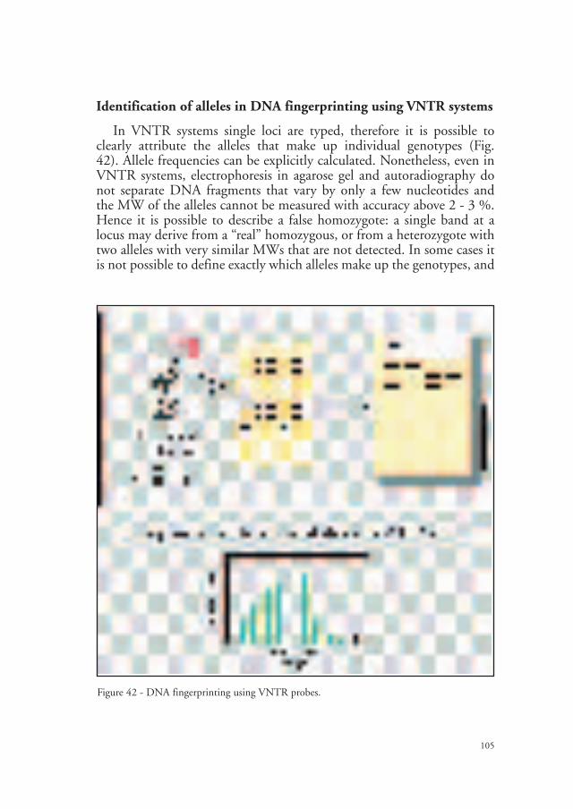
105

Identification of alleles in DNA fingerprinting using VNTR systems

In VNTR systems single loci are typed, therefore it is possible to clearly attribute the alleles that make up individual genotypes (Fig. 42). Allele frequencies can be explicitly calculated. Nonetheless, even in VNTR systems, electrophoresis in agarose gel and autoradiography do not separate DNA fragments that vary by only a few nucleotides and the MW of the alleles cannot be measured with accuracy above 2 - 3 %. Hence it is possible to describe a false homozygote: a single band at a locus may derive from a “real” homozygous, or from a heterozygote with two alleles with very similar MWs that are not detected. In some cases it is not possible to define exactly which alleles make up the genotypes, and

Figure 42 - DNA fingerprinting using VNTR probes.

106

the binning system becomes necessary. As of 1994 the SLP systems have been progressively substituted by microsatellite analysis.

Identification of alleles in DNA fingerprinting analysis with microsatellites

STR systems, amplified with PCR and typed by electrophoresis through acrylamide gel, permit the identification of the MW of each allele present at each locus with greater precision, above all if electrophoresis is done through automated sequencers. Electropherograms (see DNA analysis using automated sequencers) determine the MW of STR alleles with great precision. Microsatellite loci usually have a number of alleles per locus that is inferior to the alleles present at minisatellite loci. Moreover, STR alleles are better characterised: they vary by two, four or six nucleotides, in loci made up of a repeat unit of dinucleotides, tetranucleotides or esanucleotides. Therefore, STR loci are well characterised: the genetic structure of the repeat can be described through nucleotide sequencing, the alleles present in the population can be characterised exactly indicating the number of repeats that they are made up of, and therefore defining their length and MW precisely; the loci can be mapped on chromosomes, and therefore their reciprocal linkage relationship can be defined with precision. The risk of contamination is one of the drawbacks, though in MLP systems it is virtually non-existent, and the problem of allelic dropout is another.

STATISTICAL ANALYSIS OF DATA

Frequency distribution

Results of forensic genetic analysis (identification of individual genotypes) are used to determine the probability of individualisation in samples and to reconstruct the distribution of allele frequencies in populations from where the samples were taken. Several problems may arise in evaluating these results. For example: What is the uncertainty associated with the estimated allele frequencies in reference populations? In what manner can allele frequencies be used to correctly calculate genotypes frequencies? Are the observed genotype frequencies a good estimate of the frequencies in reference populations? What is the probability of observing a genotype G in an individual sampled at

107

random in the reference population? The theory of probability and statistical analysis methods furnish the instruments to correctly perform these calculations. Statistical analysis provides the arithmetic procedures to correctly estimate the parameter values of the population using data obtained from sample. A sample survey should be random, representative, stratified and have the appropriate size. Nonetheless, during forensic genetic procedures it is seldom possible to work on representative samples from well characterised reference populations. Data available from databanks are often used.

Statistical data are always obtained from limited samples extracted from populations that include all living individuals. A random sampling is a collection of individuals selected at random, that is chosen in such a way that each of the components of the population has the same probability of being included in the sample. The size of the sample is indicated with an n. The sample is measured to obtain the values of certain set characters Xi (for example, the allele frequencies at a panel of microsatellites). The values of character X takes in the sample survey are the so-called observations, and are indicated by x1, x2, x3, …, xn. Observations and statistical data are represented in graphic or tabular forms. An allele frequency table can be represented graphically as a bar graph or a histogram (Fig. 43). Observations have a frequency distribution that is described in mathematical terms (for example: normal distribution, Poisson distribution). Every distribution frequency is described in terms of the estimated “parameters” of the population

Figure 43 – Frequency distributions.

108

from where the data were extracted: the central value of a series of values (mean, median, mode), the dispersion measurements of observations that differ from the mean (variance, standard deviation, percentiles).

Procedures of statistical analysis allow one to estimate the parameters of a distribution, to evaluate the precision of the estimates, and to test the significance of hypotheses. Estimates of the parameters are obtained through analysis of the samples. Statistics serve to compare the values observed with the expected values obtained from frequency distributions. A frequency distribution assigns a probability to every possible value of variables. For example, in throwing a coin one assumes that the probability of it coming up “heads” is the same probability of it coming up “tails” (50%). In population and forensic genetics, one assumes that the observed alleles and genotypes were taken from a population with a binomial distribution (Bernoulli distribution), that describes the frequency distribution of a series of independent events, each of which has two possible results: a1 (with probability p) or a2 (with probability q = 1 - p). If p = q = 0.50, we can calculate the probability of obtaining the events : a1 a1 = p x p = 0.25; a1 a2 = a2 a1 = 2 x p x q = 0.50; and a2 a2 = q x q = 0.25, that correspond to the proportion of estimated genotypes on the basis of Mendel’s laws. If p # q, the binomial distribution describes the estimated genotype proportions in a population in Hardy-Weinberg equilibrium. A binomial distribution B is defined by its probability density function (pdf ):

Pr(x|n, p) = [n ! / x !(n - x)!]px(1 - p) (n-x)

The probability (Pr) that an event (that has probability p) occurs x times in a sample size n, is equal to pdf, with :

n!, x! and (n - x)! = n, x, and (n - x) factorial (for example, if n = 3, 3! = 3 x 2 x 1 = 6).

A binomial distribution B(n, p) and its pdf are described by the “parameters” n and p. The mean of B(n, p) is µ = np. The variance of B(n, p) is σ2 = np(1 - p). The standard deviation (SD) is the square root of the variance. If we sample n = 100 individuals from a population in which the genotype G has the frequency p = 0.20, one expects to obtain approximately m = np = 20 G, with variance σ2 = np(1 - p) = 20 x 0.8 = 16, and with SD = 4.

For example: laboratory analyses have compiled a list of genotypes, obtained by identifying the alleles a1 that are present in a sample of n = 50 individuals at locus A (VNTR or STR). The results are presented

109

in a tabular format or as a frequency distribution. Let’s consider that in the sample analysed, 11 individuals were present with genotype a1a2. The genotype frequency in the sample is calculated as a proportion: 11/50 = 0.22. Is this frequency a correct estimate of the genotype frequency of a1 a2? If the genotype G = a1a2 has frequency p = 0.22, the probability of observing x = 11 G out of n = 50 individual sampled is given by binomial pdf B(50, p):

Pr(x = 11|p) = [50! /11! (50 - 11)!]p11(1 - p)(39) = 0.22

If the probability of an event is very small, the binomial distribution corresponds to the Poisson distribution:

Pr(x|λ) = λxe-λ/x!

In this distribution the mean equals the variance: m = σ2 = λ. If every event has more than two possible results, the distribution becomes multinomial.

A binomial distribution with B(n, 0.5) is symmetrical. If n is great the binomial distribution becomes normal: N(µ,σ2) (Fig. 43). When a normal distribution is continuous, the areas under the distribution curve is equal to 1, that is, the probability that all the events occur is 100%. There are infinite normal distributions that correspond to all the possible means and variances, but they can be standardised to have mean = 0 and variance = 1. Standardisation is obtained by transforming the values of x, belonging to N(µ,σ2), in the variable z = (x - µ)/σ2. A standardised normal distribution N(0, 1) has 95% of its values within two SD of the mean. The values of z = +/- 1.96 includes 95% of the normal distribution. Therefore, there is a 5% probability that a standardised variable normally distributed has values > or < than 1.96, i.e. outside the two SD of the mean (Fig. 43). The pdf of a standardised binomial variable is: z = (x - np) / √np(1 - p).

This formulation allows us to calculate the probability of binomial events. However, in order to apply the binomial distribution to forensic genetics it is necessary to calculate the distribution parameters starting from the sample. Therefore it is not necessary to deduce the probability of an event given by a theoretical distribution where the value of the parameters are known, but rather estimate the value of the parameters of a frequency distribution to which the observed events belong.

In a pdf form the probability of x has been conditioned by p:

Pr(x = n|p)

It is possible to estimate the probability of p, conditioning on a fixed value of x:

110

L(p|x) = k(p)(x) (1 - p)(n - x)

In this form the function is called: “likelihood” of p given x = 11, with k = proportional constant that substitutes the expression [50! / 11! (50 - 11)!]. The distribution of L is equal to a binomial distribution, but the vertical scale depends on the value of k. In this case, the distribution of L has a maximum at p = 0.22, that is to say 0.22 is the most probable value of parameter p on the basis of the data. Utilising the maximum likelihood (ML) method, one can identify this value as an estimate of the parameter. In general, L (p) = x | n, if the parameter to estimate p belongs to a binomial pdf. Therefore 11 / 50 = 0.22 is a good estimate of the frequency of the genotype G in a population. There are also more complicated situations in which the parameter does not belong to a binomial distribution and therefore must be estimated through ML.

Estimation of confidence intervals

Confidence intervals indicates the accuracy of point parameter estimates, and are calculated in such a way that, when an experiment is repeated several times, the true parameter value is comprised within an interval a pre-specified percentage of times. For example, a confidence interval of 95% affirms that the parameter value is comprised within the interval in 95% of the samples. In forensic genetics it is important to calculate the variation intervals of allele frequencies: the rarest allele frequencies can be determined accurately only be examining hundreds, or thousands of samples, which is something that seldom occurs. Therefore it is necessary to indicate the confidence interval of the estimates. Any standardised variable, normally distributed with mean m and variance σ2 = np(1 - p), has values comprised between m +/- 1.96 with 95% of probability. The standard error of the mean, that indicates how much the estimate varies from the mean is: sem = s / √n. The confidence interval that includes 95% of the mean values of a variable that, with probability p, occurs x times out of a total of n events is:

m +/- 1.96√ p(1 - p)/n

This formula is valid only if the sample is sufficiently large, that is, if both np and n(1 - p) > 5.

The formulas for confidence levels can be used to determine the necessary size of the sample in order to obtain a prefixed level of precision in the estimates:

111

n = (1.96 / L)2p’(1 - p’)

It is necessary to analyse n individuals, if one wishes to obtain an allele frequency estimate that is accurate with a 95% confidence of +/- L. The expected frequency in the population is p’.

When a locus has multiple alleles, the confidence intervals of single alleles are not equivalent to the multiple interval. To obtain a correct simultaneous calculation of the confidence intervals for multiple alleles, the Bonferroni correction must be applied. If the estimated frequencies of k alleles at a locus with a confidence of (1 - α ) x 100% (α = significance level = 1- p; usually p = 95% or 99%), the Bonferroni correction is = (1 - α/k) x 100%.

Hypothesis testing

Procedures to calculate significance tests are based on the comparison between the expected results given a null hypothesis (HO), and the observed results. The simplest test for categorical data is the chi-square test:

χ2 = Σ(0 - E)2 / E

with:

0 = number of observations;

E = number of expected observations given HO

HO is rejected if the value of χ2 is greater than a reference value calculated by the theoretical distribution χ2, with M degrees of freedom (df) and at the prefixed significance level (α). For example, in the distribution of χ2 with 1 df, a value > 3.84 occurs < 5% of the times if the null hypothesis is true. Values greater than 3.84 would lead to the rejection of the null hypothesis at a 5% significance level, that is with a P value of 5%. The χ2 test can give false results when the number of expected events is low. In these cases it is better to use the exact test. The exact test assume that the null hypotheses is true and calculate the probability of the observed result or of the most extreme values (and therefore less probable) than the observed result. If the probability of these values is low, the null hypothesis is false. Statistical analysis of allele frequencies in population genetics and forensic genetics can test if a reference population is in HWE and LE. These analyses can be carried out using any of the numerous softwares available on the market.

112

Estimating allelic and genotype frequencies

The aim of forensic genetics is to verify the hypothesis that a DNA fingerprinting is univocally associated with a certain individual, or that the DNA fingerprinting of an offspring derives from DNA fingerprinting of two hypothetical parents. DNA analysis allows us to draw the following conclusions:• it is not possible to state with certainty whether the samples have

identical DNA fingerprinting (inconclusive results). This may occur for different reasons: the samples could be degraded, contaminated, the genetic variability could be insufficient. The analyses can be repeated with the same or different methods in an attempt to improve the results. The results of an inconclusive analysis cannot be utilised; it is as if the analyses were not carried out;

• the fingerprinting is different and therefore must have originated from different individuals (exclusion); an exclusion has an absolute value and does not require further analyses nor discussion;

• the DNA fingerprintings are matching (inclusion) and can confirm the hypothesised associations.In the third case the problem becomes the following: What is the

meaning of matching? In other words: What is the probability that two different individuals in a reference population have identical DNA fingerprints by chance? If, for the sake of argument, samples submitted for genetic testing are from individuals belonging to a small population, reproductively isolated for many generations, therefore with high values of inbreeding and reduced genetic variability, the two individuals could have a significant probability of sharing the same DNA fingerprints. In this case, a conclusion of genetic identity (inclusion) could be wrong.

Two samples may appear genetically similar for the following reasons:• because the two samples come from the same individual;• by coincidence: the two samples come from two individuals that are

genetically similar by chance;• by mistake: the two samples come from two individuals that are

genetically different, but resulted similar in consequence of errors made during the analyses (samples identified badly, errors of analysis, inadequate laboratory methods, etc.).How can one distinguish these three possibilities from each other?

Quality control of analyses carried out in the forensic genetics laboratory can exclude the third case. Considerations regarding population genetics may exclude the second case. If only one or a few individuals in a

113

population can have by chance the identified DNA fingerprinting, then a coincidence is extremely improbable. If, on the contrary, a part of the population shares the same DNA fingerprints, then two individuals can be identical by coincidence. For example, a false parent could have by chance the same genotype as the biological father. The problem becomes: What is the probability that two individuals of a population have the same DNA fingerprints by chance? Or, one may ask: What is the probability of finding that particular DNA fingerprinting if the putative father is the true father, compared to the probability of finding the same DNA fingerprinting in someone else, and not the putative father, is the true father? The answer depends on the frequency of that particular DNA fingerprint in the reference population.

To determine the frequency of a DNA fingerprinting it is necessary to analyse a representative sample of individuals of the reference population, and count the number of times in which each genotype, that is, every DNA fingerprinting occurs. If loci with few alleles are examined, identical genotypes would appear quite frequently. For example, if a locus has only two alleles, there will be only three genotypes in a population, each of which will probably be shared by many individuals. In this case it is sufficient to examine a small sample survey of individuals to obtain a precise estimate of the frequency of the three genotypes. If loci with many alleles are examined, the number of possible genotypes would increase. In this case it is necessary to make a much bigger sample survey to obtain precise estimates of the genotypes frequencies. When DNA fingerprinting is composed of hypervariable multiple loci, the number of possible genotypes becomes very high and it is improbable, if not impossible to find them all in the individuals of the population. In this case an estimate of the allele frequencies becomes difficult and the estimate of genotype frequencies becomes impossible even if examining a very large sample size. For example, if human minisatellites are studied with MLP, each locus can have up to 50 alleles, that can combine and produces 1275 different genotypes. If four loci each with 50 alleles were examined, the number of possible genotypes would be (1275)4, that is, about 2.6 trillion. As there are presently about 6 billion human beings, it is evident that the majority of these genotypes simple do not exist. A direct estimate of the frequency of these genotypes is not possible.

Therefore it is necessary to obtain indirect estimates of (expected) genotype frequencies. These estimates can be calculated on the basis of the theory of population genetics. If we presume that a population is in HWE and in LE, then it is possible to estimate the genotype frequencies on the

114

basis of allele frequencies that have been observed in the population. The total number of alleles present in the population is much smaller than the number of genotypes. Thus, it is much simpler to estimate the allele frequencies. Real populations always have a finite size that, in some cases, can be very small. Mating is often not random, but occurs on the basis of certain criteria regarding choice of partners (for example, in human beings, the choices can be made on the basis of social class, religion, ethnic group; in animal species, the choice of partners is often made on the basis of morphological characters that signal the fitness of the reproducers), there can be migration and exchange of individuals among differentiated populations. Most human populations and many “populations” of animals reproduced in captivity, are in reality admixture of individuals who originate from different and genetically differentiated populations. In these cases, the populations are not indistinct groups of individuals but are stratified, that is, they are structured in subgroups that can be genetically differentiated from each other. It is possible that a structured population, that is divided into subpopulations, is not in HWE. Obviously, individuals that belong to each subgroup will be less genetically differentiated among themselves than what one could expect from a population if it was not structured. Individuals in a subgroup may not be in LE.

Estimates of genotype frequencies in structured populations do not necessarily present practical problems. In fact:• deviation from HWE and LE may be slight and not invalidate the

estimates of genotype frequencies calculated utilising estimates of allele frequencies;

• the effects of structure in populations are foreseeable and can be corrected mathematically. In a structured population one expects to find more homozygotes and fewer heterozygotes, than expected in a Mendelian population. The effect of structure in a population on LE is to increase the correlation among some loci and diminish it among others. After having collected empirical data on genetic variability in a population, one can quantify the deviation between HWE and LE, and therefore correct errors made in estimating genotype frequencies. It is possible to reconstruct subgroups present in a population, even without knowing the composition beforehand.

Estimates of the allele frequencies at codominant loci

Mendel derived his laws from observations on the frequencies of phenotype characters whose expression is controlled by relationships of

115

dominance/recessivity. The dominant alleles impede the expression of recessive ones, which cannot be directly observed. There are statistical methods that can be used to estimate the allele frequencies of loci with dominant/recessive alleles. However, direct analysis of DNA allows both the alleles present at heterozygous loci to be detected (with the exception of DNA multi-locus fingerprinting where identification of single alleles is problematic), which can be treated as codominant loci. The analysis of codominant loci permits the calculation of allele frequencies directly from counting the genotypes present in the sample, with the following formula:

p(a1) = p(a1a1) + 1/2Σpaxa1

with :

p(a1) = frequency of allele a1

p(a1a1) = frequency of homozygous genotype a1a1

p(axa1) = frequency of heterozygous genotypes that contain the allele a1

If a locus only has 2 alleles, a1 and a2, there will only be one heterozygote genotype; a1a2. However, if the locus has more than two alleles (multiple alleles) there will be two or more possible heterozygte genotypes. The homozygotes contain two copies of the same allele, while the heterozygotes contain only one copy of every allele. Therefore it is necessary to divide the frequencies of the heterozygotes by 2.

In a system with two codominant alleles, this formula is the same as the following:

p(a1) = [2(a1a1) + (a2a1)]/2n = pp(a1) = 1 - p(a1) = q

with: (a1a1) = number of homozygotes in the sample; (a2a1) = number of heterozygotes in the sample; n = total number of individuals analysed. The standard error of the estimates is: √(pq/2n)

Estimates of allele frequencies in minisatellites analysed with MLP systems

In DNA multi-locus fingerprinting, identification of single alleles is problematic. In practice, two fragments are identified as “matching” if they have molecular weight that is determined within 3 units of standard deviation in either direction. In well-calibrated electrophoresis systems, every fragment has a standard deviation that corresponds to

116

approximately 0.6% of its molecular weight. Therefore two fragments are matching if they have the same MW ± 2.0 - 2.5% of deviation from the mean MW. Two matching fragments are assigned to the same “allele”. In human forensic genetics the “alleles” of similar MW are grouped into the same bin. Every bin must contain at least 5 different alleles. Then a calculation is made of the bins frequency to which the “alleles” belong. In forensic genetics of CITES species, an adequate database of reference populations is almost always missing. Every so defined “allele” corresponds to a bin. The allele frequencies and the bin frequencies in reference populations are equivalent. The frequency of every fragment is simply calculated as a proportion: number of samples in which the fragment is present / the total number of samples analysed.

Estimates of genotype frequencies at multi-locus systems

The Hardy-Weinberg law calculates the expected genotype frequencies at a single locus, utilising the allele frequencies estimated in the sample:• homozygous genotypes: p(a1a1) = p(a1)2: the frequency of the

homozygous genotype a1a1 is the same as the square of the allele frequency a1

• heterozygous genotypes: p(axa1) = 2p(a1)p(ax): the frequency of the heterozygous genotype that contains allele a1 is the same as double the product of the allele frequencies.The genotype frequencies calculated through allele frequencies match

the genotype frequencies of the population only if the population is in HWE. In a population in equilibrium, the allelic and genotype frequencies do not change from one generation to the next. Evolution (selection, mutation, migration) can changes allele frequencies from one generation to the next. In an evolving population, the expected genotype frequencies cannot be estimated directly through the allele frequencies and the Hardy-Weinberg law.

DNA fingerprinting profiles used in forensic genetics are almost always determined using multi-locus systems. It is possible to estimate the frequency of a multi-locus genotype as a product of alleles frequencies that are present at each locus that makes up the profile. If the multi-locus system is made up of loci A (with alleles a1 and a2), B (with alleles b1 and b2), and C (with alleles c1 and c2), the frequency of the multi-locus genotype is calculated through the “product rule” that generalises the Hardy-Weinberg law:

p(ABC) = 2H p(a1)p(a2)p(b1)p(b2)p(c1)p(c2)

117

That is, the frequency of the genotype ABC is the same as the product of the frequencies of the alleles that it is made up from, multiplied by 2H, with H = number of loci that are heterozygous in the profile. This estimate is correct only if the segregation between all alleles present in the profile is independent, that is, if the population is in HWE and if all alleles are in LE. These assumptions are seldom satisfied (and also quite problematic to verify) in real populations of finite size. Nonetheless, deviations from HWE and LE are not so great as to invalidate the estimate of the genotype frequencies.

Stratification. If a population (not in HWE) is made up of differentiated subpopulations, each of which is in HWE, then the genotype frequencies can be calculated by the allele frequencies in the total population introducing the correction factor q. If the allele frequencies of the subpopulations are known, then the genotype frequencies are calculated exactly as above without having to introduce any correction.

Confidence intervals for multi-locus genotypes. If the size of the sample survey is large and if the genotype frequency at locus P is not very much smaller than 0.5, then the binomial distribution B(n, P) of P tends to a normal distribution and the confidence interval at 95% for P is calculated:

P +/- 1.96√P(1 - P) / n

However the confidence intervals of genotypes at single loci are of limited use, as we are interested in defining the characteristics of the frequency distributions of multi-locus genotypes. The multi-locus confidence intervals require the application of complex statistics, and can be calculated through specific software. If the frequency of the multi-locus genotype P is small, confidence intervals can often be (P/10, 10P). Therefore it is impossible to estimate small frequencies in small samples with precision.

PROBABILITY

Calculations that provide estimates of genotype frequencies are based on the concepts of probability. What is the probability that two samples that have similar genetic profiles belong to the same individual? What is the probability that a putative father is the biological father when all the alleles of the child have been identified in the mother and in the putative father? The theory of probability is used to answer these questions. The objective of calculating the probability is to quantify uncertainty, that is to assign a value of probability to an uncertain event through statistical

118

analysis. Uncertainty derives from complexity, which makes it impossible to check all the cause-effect connections and to have all the necessary information available to understand the true processes. Probability is a measure of uncertainty expressed as a number that varies from 0 to 1. There are different concepts of probability. Probability can be determined subjectively, objectively or empirically. Subjective probability is based on experience, which allow a likelihood ratio to be assigned to events. Objective probability is based on data from experiments that allow the frequency of an event to be calculated. Empirical probability is based on information acquired from an analysis of the data already available.

The frequency theory of probability

The probability p of an event H depends on the number of times (n) the event occurs on the total number of tests (N). The probability p of H corresponds therefore to its frequency:

pH = n(H) / N

This definition is based on the assumption that all the events are equally probable. Obviously, if the number of tests is small, the estimate of pH will be uncertain. The “law of large numbers” guarantees that repeating the tests many times (tending to infinite), pH will be determined precisely. In classic statistics the value H can be determined only experimentally, because there are no laws of universal nature that guarantee the equiprobability of events. Even in the tossing of a coin, there are no laws of physics that guarantee that p “heads” = p “tails” = 50%.

If we toss a coin only a few times, ph # pt (h = heads; t = tails). If we toss a coin a great number of times (tending to infinite), ph = pt (but this must be experimentally verified). The result of an event (random variable), can has two values (true or false) or more numeric values. Classic statistics is of little use in determining the uncertainty of events that cannot be experimented. For example: What is the probability that it will rain tomorrow? What is the probability that the genotype of this sample corresponds to this individual?

The subjective theory of probability (Bayesian statistics)

The probability p is an estimate of likelihood that the event H occurs. We can have convictions (subjective) or information (objective, even though not exactly quantifiable) that an event may more or less occur frequently.

119

Circumstances, that do not correspond to the frequencies determined experimentally, allow the probability of an event to be assigned. From this point of view, the probabilities assigned to an event are conditional, that is, they are valid only in the presence of certain circumstances. For example: ph = pt = 0.5, only if we know that a coin has heads on one face and tails on the other, that the two sides are of the same weight, that the coin is tossed in such a way as to randomise the events (randomisation: procedure of maximising uncertainty; maximum uncertainty: when all the events have exactly the same possibility of occurring, that is they have the same likelihood). If we know that ph = pt = 0.5, then we can expect that in reality ph is equal to pt if we toss a coin a great number of times. Prediction of the result from tossing a coin does not depend on a law of physics, but on the conditions associated with the toss.

In what way can we determine the probability of an uncertain event in which its frequency cannot be experimented? That is, what is the Pr(H|E) = the probability that an event H occurs given the evidence E? The factors that influence PrE can be many, for example: Pr(H|S,C, I), where S, C and I indicate the data (that is, the quantifiable observations) and the information (that is, data that is not exactly quantifiable) that are important in determining PrH. The data and information constitute the evidence. If we consider that all the probabilities can be influenced in some manner, then Pr(H|E) = Pr(E), and the two notations are equivalent.

The laws of probability

• The first law of probability: "the values of probability range from 0 to 1".

0 > Pr(H|E) < 1

The complementary probability of Pr(H|E) is: 1 - Pr(H|E). If E occurs (occurred or certainly will occur), then Pr = 1, and its complementary probability will be 1 - 1 = 0.

• The second law of probability: "two events are reciprocally exclusive if the occurrence of one (h = heads) excludes the occurrence of the other (t = tails; the result of the coin toss is either heads or tails)". The probability that either one or the other of the two mutually exclusive events occurs, is given by the total of their respective probability (addition rule):

Pr(h or t|E) = Pr(h|E) + Pr(t|E) = 1.

120

The complementary probability of an exclusive event is:

Pr(t|E) = 1 - Pr(h|E).

The two events are exhaustive.

• The third law of probability: "two events are independent if the occurrence of one does not influence the occurrence of the other". The probability that both occur (one and the other) is given by the product of their respective probability (product rule):

Pr(A and B|E) = Pr(A|E)Pr(B|A, E).

The following formulas are equivalent:

Pr(A and B) = Pr(A)Pr(B|E) = Pr(B)Pr(A|E) = Pr(A)Pr(B)

In this case the two events are statistically independent (conditional on E). Two events can be independent assuming one hypothesis, but dependent by assuming another.

Example: Locus A has allele a with frequency p = 0.2; locus B has allele b with frequency p = 0.3. The two loci are independent. The probability of obtaining a genotype with both alleles a and b is calculated by the product rule: Pr(a and b) = Pr(a)Pr(b) = 0.2 x 0.3 = 0.6.

Example. A population made up of two subpopulations: 25% A and 75% C. The genotype G is present in 4.8% of the individuals in the population A. What is the probability that a person chosen at random from the total population comes from the subpopulation A and has the genotype G? the probability is: Pr(A and G) = Pr(A)Pr(G|A) = 0.25 x 0.048 = 0.012.

• Events partially associated. Two events can be only partially independent and have something in common in this case:

Pr(A or B) = Pr(A) + Pr(B) - Pr(A and B), that is, the probability an event partly depends even on the occurrence of the other event. The probability that both events will occur is:

Pr(A and B) = Pr(A|B)Pr(B) = Pr(B|A)P(A), where Pr(A|B) is the conditional probability that A will occur if B has occurred.

Example. The probability of obtaining a genotype with only allele a or only allele b or with both allele a and b, at locus A is: Pr(a or b) = Pr(a) + Pr(b) - Pr (a and b) = 0.2 + 0.3 - 0.06 = 0.44.

121

• The law of total probability. If two events A and B are mutually exclusive and absolute (B =1 - A), the probability of an event H that depends on A and B is:

Pr(H) = Pr(H|A)Pr(A) + Pr(H|B)Pr(B)

Example. A population is made up of three subpopulations: 83.47% A, 12.19% B, 4.34% C. The genotype G is present in the three subpopulations with the frequencies 0.013, 0.045 and 0.039, respectively. What is the probability of finding G in an individual taken at random from the total population? The probability is = 0.013 x 83.47 + 0.045 x 12.19 + 0.039 x 4.34 = 0.018.

Bayes’ Theorem

We have 52 playing cards and we want to calculate the probability of extracting a King. There are 4 Kings in each set of cards, so the probability of extracting a King is 4/52. Now let’s calculate the probability of extracting a Red card which is also a King. That is: if the card is a King, what is the (conditional) probability that it is Red: Pr(Red card|King). A set of cards is made up of 50% Red cards and from 50% of Black cards, therefore Pr(Red card|King) = 2/4 = 0.5. The inverse probability is the possibility of extracting a King in a set of cards that are all Red: Pr(King|Red card) = 2/26.

Bayes’ theorem (formulated by Reverend Thomas Bayes; 1702 - 1761) puts these two probabilities in relation with each other. Let’s identify the cards: A = Red card, B = King. Bayes’ theorem states that :

Pr(B|A) = Pr(A|B)[Pr(B) / Pr(A)]

In this formula the Bayes’ theorem requires knowledge of two non-conditional prior probabilities, that are: Pr(A) = Pr(Red card) = 50% = 26 Red cards/52 cards in a set; Pr(B) = 4 Kings/52 cards in a set. Moreover, it is necessary to know the value of a prior conditional probability, that is: Pr(A|B) = Pr(Red card|conditioned by the fact that it is a King) = 2/4. By applying Bayes’ theorem we can calculate the probability of extracting a King conditioned by the fact that the card is Red:

Pr(B|A) = (2/4) [(4/52) / (26/52)] = 2/26

The unknown conditional probability (posterior) can be calculated by the conditional probability and by the two non-conditional prior

122

probabilities. In this case the unknown probability could have been calculated directly, knowing that 50 % of the cards are Red, including the two Kings out of four. There are numerous cases in which posterior probabilities are not known, while prior probabilities are either known or hypothesised. Bayes’s theorem estimates the values of probability and update them on the basis of information provided by the evidence. We have a prior estimate of the probability of an event occurring, that is combined with the conditional (likelihood) probability of the evidence in the case an event occurs, to obtain an updated probability (posterior) of the event given the evidence. The information known prior to the event is called “prior probability”; the information known after the event is called “posterior probability”.

Bayes’ theorem can be expressed in the following form:

Pr(Hp|E, I) / Pr(Hd|E, I) =[Pr(E|Hp, I) / Pr(E|Hd, I)] x [Pr(Hp|I) /Pr(Hd|I)]

with: E =evidence; I =other information that influences the Pr of the event Hp and the Pr of the alternative event Hd.

In this way, Bayes’ theorem is written in the form of odds. If we know that the probability of H is Pr(H), the odds O is in favour of H is:

O(H) = Pr(H) / {1 - Pr(H)}

We know that Pr(H) + {1 - Pr(H)} = 1; O(H) may vary between 0 (if H is false) to infinite (if H is true). When the odds are down (e.g.: 1 to 5) it inversely corresponds to the odds that are up (e.g.: 5 to 1). When the odds one way or the other are equal = 0.5, then we say they are “even”. The conversion of odds into probability is:

Pr(H) =O(H) / 1 + O(H)

Example: if O(H) = 1/5, Pr(H) = 1/5/1+1/5 = 0.17

Bayes’ theorem expressed in the form of odds allow the posterior probabilities of an event to be calculated [posterior odds = Pr(Hp|E, I) / Pr(Hd|E, I)], as the product of two relationships:

• the relationship between conditional probabilities of the evidence, given the event and an alternative event, which is called the likelihood ratio = [Pr(E|Hp, I) / Pr(E|Hd, I)];

• the relationship between two prior probabilities = [ Pr(Hp|I) / Pr(Hd| I)].

123

APPLICATIONS OF BAYESIAN STATISTICSTO FORENSIC GENETICS

The Bayesian approach is either explicitly on implicitly understood in resolving questions regarding forensic genetics (see, for example, the technical report U.S.A. National Research Council - NRC, 1966). We have followed the text by Evett and Weir (1998) in presenting the applications of the Bayesian model.

Identification

Let’s assume that a forest warden finds the remains of a deer carcass, apparently killed out of the hunting season (or in a protected area), and then confiscates portions of the meat kept in a freezer by a hypothetical poacher. On the basis of a series of information, the forest warden believes that the hypothetical poacher is the person responsible for killing the deer. Biological samples from the deer carcass are taken (material evidence) as well as from the frozen meat (the suspect). DNA fingerprinting profile analyses are carried out on both these samples. The samples indicate identical DNA fingerprinting profiles. The problem is to establish whether the two samples belong to the same individual and whether, as a consequence, the hypothetical poacher can be accused of a crime. Obviously, whatever the results provided by the genetic testing procedures, they do not constitute evidence that the accused effectively committed the crime. The suspect could furnish plausible explanations for having had in some manner and in good faith the confiscated meat in his freezer.

The Bayesian model allows evaluating two alternative hypotheses, mutually exclusive and absolute:• Hp: the frozen meat belongs to the deer carcass;• Hd: the frozen meat does not belong the deer carcass;

Genetic evidence G is provided by DNA fingerprinting:• Gs: the DNA fingerprinting of the frozen meat (suspect);• Gc: the DNA fingerprinting of the carcass (material evidence);

In this case the laboratory analyses state that: Gs = Gc.The next step is to evaluate the non-genetic information I, that is all

the other information that can sustain the accusation (Hp).Before the DNA analyses, the probability of Hp was conditioned

only by I: Pr(Hp|I). After the DNA analyses, the probability of Hp is conditioned by Gs, Gc and I: Pr(Hp|Gs, Gc, I). To estimate Pr(Hp) it is

124

necessary to have at least one alternative hypothesis Hd. To calculate the probability of the two alternative hypotheses we can use Bayes’ theorem, expressed in the form of odds. Therefore we must evaluate:• The prior odds in favour of Hp: Pr(Hp|I) / Pr(Hd|I);• The posterior odds in favour of Hp: Pr(Hp|Gs, Gc, I) / Pr(Hd|Gs, Gc, I).

The prior probabilities must be known beforehand. The posterior probabilities can be calculated using Bayes’ theorem. Let’s define evidence as E = (Gs, Gc):

Pr(Hp|E, I) / Pr(Hd|E, I) =[Pr(E|Hp, I) / Pr(E|Hd, I)] x [Pr(Hp|I) / Pr(Hd|I)]

This formula means that one must calculate:• What is the probability Pr(E|Hp, I) of the evidence (DNA fingerprinting)

given that Hp is true?• What is the probability Pr(E|Hd, I) of the evidence (DNA fingerprinting)

given that Hd is true?The relationship between the two posterior probabilities is the

likelihood ration LR = Pr(E|Hp, I) / Pr(E|Hd, I). The posterior probabilities are calculated by multiplying the prior probabilities by LR.

LR = Pr(E|Hp, I) / Pr(E|Hd, I) =Pr(Gs, Gc|Hp, I) / Pr(Gs, Gc|Hd, I)

By applying the third law of probability LR ca be extended, that becomes:

LR = Pr(Gc|Gs, Hp, I) / Pr(Gc|Gs, Hd, I) x Pr(Gs|Hp, I) / Pr(Gs|Hd, I)

The terms: Pr(Gs|Hp, I) and Pr(Gs|Hd, I) indicate the probabilities of observing the genotype Gs independently from genotype Gc. Therefore: Pr(Gs|Hp, I) = Pr(Gs|Hd, I), as the likelihood of the two alternative hypotheses does not provide information regarding the likelihood of the genotype Gs. Therefore:

LR = Pr(Gc|Gs, Hp, I) / Pr(Gc|Gs, Hd, I) x 1 = Pr(Gc|Gs, Hp, I) / Pr(Gc|Gs, Hd, I)

As we are certain that the genotype is Gc in the case that Hp is true, then Pr(Gc|Gs, Hp, I) = 1, therefore:

LR = 1 / Pr(Gc|Gs, Hd, I)

All that remains to do is to assign the probability of Gc in the case that the sample belongs to another individual and not to the dead deer

125

that was found by the forest warden. This probability depends on I (the circumstances). If we assume that Gs does not influence the uncertainty of Gc, given that in the hypothesis they belong to two different individuals (an assumption that in some cases can be false, for example if the two samples come from related individuals), then:

Pr(Gc|Gs, Hd, I) = Pr(Gc|Hd, I), and therefore:

LR = 1 / Pr(Gc|Hd, I)

How can a value be assigned to a denominator? What is the probability of observing the genotype Gc = Gs = G, if the two analysed samples do not belong to the same individual? The answer depends entirely on I. In this case it is necessary to identify the group of individuals from where G originates, that is, the population from where the deer came from. It is then necessary to obtain genetic information on a representative group of individuals of the reference population, and use this information to estimate the population parameters, using statistical methods. Let’s presume that all the above has been done and that we know that the genotype G is present in the population with of frequency P, that corresponds to the probability of the denominator. Then:

LR = 1 / P

For example, if P = 0.01 = 1/100, then LR = 100, which means: “the evidence is 100 times more probable if the sample of meat and the sample taken from the carcass belong to the same deer than it is if they belonged to two distinct deer (not related) from the same population”. This conclusion is based on the information than conditions it: If the two samples come from two different individuals, are they or are they not related? How do we define the population from where the suspect sample came from? Is it a genetically homogeneous population or made up of subpopulations? Does every individual of the population have the same probability of being killed? The assumptions used to condition the calculation of the probability must be made explicit, and if new circumstances require it, they must be modified. One arrives at the same conclusion (LR = 1 / P) using a frequency model, but in this case the underlying assumptions are not explicit, and therefore it is not possible highlight the subjective elements that condition a calculation of the probability

The three principles of interpreting evidence (Evett and Weir, 1998)• To evaluate the uncertainty of every hypothesis, it is necessary to

consider at least one alternative hypothesis.

126

• The interpretation of scientific evidence is based on the answer to the question: “What is the probability of observing the evidence given the hypothesis?”

• Interpretation of the evidence is conditioned not only by alternative hypotheses, but also by the circumstances regarding the evidence that must be evaluated.The available information I on the size and isolation of a population

can significantly influence the interpretation of evidence. Let’s suppose, for example, the killed deer and the suspect sample originate from a small isolated population, made up of N individuals that do not receive immigrants for some time. The two DNA fingerprints are identical and present the genotype G. The genotype G has a frequency P in the population, that is the probability that a deer chosen at random from the population has the genotype G is = P. The prior probability that every deer of the population has been killed is Pr(Hp|I) = 1/ N, and LR = 1 / P.

The posterior probability is:

Pr(Hp|E, I) / Pr(Hd|E, I) = (1 / P) x (1 / N ) = 1 /NP

which is likely if every individual of the population has the same probability of identity P, but is unlikely if we consider possible parental relationships in a small population. Consequently, it is convenient to modify the previous formula to estimate the posterior probability as follows:

Pr(Hp|E, I) / Pr(Hd|E, I) = 1 / ΣiwiPiwhere: i = 1, N; wi are the probabilities that every individual i of the population the size N, has the same genotype of the killed deer, independently from the evidence provided by DNA, regarding the genotype probabilities of the material evidence; Pi are the individual probabilities of identity with genotype G. If all the wi are = 1 and all the P are =1, then the inverse probabilities are the same as 1 / NP, as above. Though if we know that two deer exist, that are brothers, then the probability that they have the same genotype G = 1/4 (see: Inbreeding). Presuming that all the other individual identity probabilities are = 1/100, the inverse probability becomes:

1 / (1/4 + 1/100) = 4

From the conclusion: “the evidence is 100 times more probable that the meat sample and the sample taken from the carcass belong to the

127

same deer than it is if they belonged to two distinct deer (unrelated) from the same population”, we can have the following extrapolations that are not justifiable:• the probability that the two samples come from two distinct individuals

is 1 out of 100, therefore there is 99% probability that they derive from the same individual;

• if the population is made up of 1000 individuals and P = 0.01, then one can expect to find 10 individuals with the same DNA fingerprints; this does not mean to say that each of these 10 individuals has the same probability (1 / 10) of being killed;

• is one expects to find an individual with a DNA fingerprint that has P = 0.01 in a population of 100 individuals, it does not mean to say that it is the killed deer.

Probability of exclusion

Every marker system used in forensic genetics must be sufficiently variable to allow the individualisation of the samples, but also sufficiently stable so as not to introduce mutations from one generation to the next (from parents to offspring). The probability of individualisation, that is of identifying a genotype that is unique in the reference population, increases by increasing the number of loci that are used in a multi-locus system. At the same time, the probability of exclusion increases. In a codominant system with k alleles, each of which with frequency pj in the population (i = 1, k), the mean probability of exclusion PE is given by the formula:

PE =Σk[ pi(1 - pi)]2 +ΣiΣj(i> j) pi pj {(1 - pi)3 + (1- pj) 3 + (pi + pj)[1 - (pi + pj)] 2}

In paternity testing the exclusion probability at each locus with two codominant alleles depends on the allele frequencies and on the paternal alleles that are present in the genotypes of each offspring. The exclusion test of paternity can be used to exclude that the putative father is the biological father, exclusion can be done directly when the putative father does not have the paternal alleles of the offspring at least one of the analysed loci, or if the allele patterns cannot be defined, he does have any of the offspring’s alleles. The paternal allele at each locus is identified as that allele that the offspring does not receive from the mother, and is easily identifiable with the exception of cases in which the mother and child are heterozygotes for the same two alleles. In this case, if the locus

128

has only two alleles, no male can be excluded at this locus. It is possible to calculate the exclusion probability in relation to the genotypes of three individual involved in the test: mother, child and putative father.

The exclusion probabilities are given in table 3 of paternal genotypes for every pair of mother-offspring types for codominant systems with two alleles. In these cases, the mean exclusion probability is:

PE = pq(1 - pq)

The exclusion probability of parental genotypes for every pair of mother-offspring genotypes for codominant systems with any number of alleles are contained in table 4.

The value of PE depends on the allele frequency in the markers used. Evidently, if p = 1, the gene is monomorphic and PE = 0. If p # 1, the exclusion probability increases until a value that, in a system of two codominant alleles, it reaches the maximum when p = q = 0.5. PE increases with the increase of allelic numbers. The maximum values of PE in codominant systems with k alleles with equal frequencies (l/k), are given in table 5.

If PE is estimated in multi-locus systems (each with the mean exclusion probability PE1), the mean exclusion value is (product rule):

PEm = 1 - (1 - PE1) (1 - PE1) …(1 - PEi)

This formula is valid if the markers used are statistically independent.

Table 3 - Exclusion probability for a locus with two codominant alleles. np = not possible allelic combination.

Genotypes Allele Paternal genotyes Exclusion mother/child frequencies AA Aa aa probability

AA - AA p3 0 0 x p3q2

Aa - AA p2q x 0 0 p4qaa - AA np -- -- -- --AA - Aa p2q 0 0 x p2q3

Aa - Aa p2q+pq2 0 0 0 --aa - Aa pq2 x 0 0 p3q2

AA - aa np -- -- -- --Aa - aa pq2 0 0 x pq4

aa - aa q3 x 0 0 p2q3

129

Match probability

It is the probability that a genotype corresponds to the genotype of an individual chosen at random from the reference population. When the genotypes obtained from two samples are identical: Gc = Gs = G, it is necessary to verify the probability that, given all the surrounding conditions, they belong to the same individual. Therefore we must confront the probability of two alternative hypotheses:

• Hp: Gc and Gs belong to the same individual• Hd: Gc and Gs belong to two different individuals

The relative likelihood of the two alternative hypotheses is evaluated by the LR. A database of allele frequencies of the reference population or subpopulation, can be used to estimate the genotypes frequencies. The

Table 4 - The exclusion probability of parental genotypes for every pair of mother-offspring genotypes for codominant systems with any number of k alleles.

Mother Child Exclusion Pr father Genotype Pr Genotype Pr Genotype Pr

aiai pi2 aiai pi awax (w, x # i) (1-pi)2

aiaj pj awax (w, x # j) (1-pj)2

aiaj 2pipj aiai pi/2 awax (w, x # i) (1-pi)2

ajaj pj/2 awax (w, x # j) (1-pj)2

aiaj (pi+pj)/2 awax (w, x # i, j) (1-pj -pi)2

aiak pk/2 awax (w, x # k) (1-pk)2

ajak pk/2 awax (w, x # k) (1-pk)2

Table 5 - Maximum exclusion probability (no paternity) for codominant genetic systems with k alleles

k Maximum Pr

2 3/16 0.188 3 30/81 0.370 4 129/256 0.504 5 372/625 0.595 6 855/1296 0.660 7 1698/2401 0.707 8 3045/4096 0.743 9 5064/6561 0.772 10 7947/10000 0.795

130

value of LR depends on a series of assumptions: the two individuals are or are not related; the sample used to estimate the allele frequency in the reference population is a random representative sample of the population; the estimate of the genotype frequencies is obtained through the product rule, that is valid if the allele frequencies are reciprocally independent; the population may or may not be structured. If the two genotypes are statistically independent, then LR = 1 / Pr(Gc| Hd, 1) = 1 / P.

Estimating the match probability of a single bi-allelic locus. If the sample was taken from a population in HWE, the match probability at a locus is calculated in the following manner:

1 / P = p2: if the locus is homozygote1 / P = 2pq: if the locus is heterozygote

Estimating the match probability of a multi-locus genotype. If the sample was taken from a population in HWE, the match probability of a multi-locus genotype is calculated through the product rule.

In some cases the two genotypes are not independent because of family ties, or because of inbreeding within the population or subpopulation. In confronting the genotypes of two individuals 4 alleles at each locus are involved (two maternal alleles and two paternal ones), that may, partly or totally be ibd. Assuming that the parents are not inbred, it is possible to calculate the ibd probability for couples of related individuals. From these probabilities it is possible to find the equation to calculate the match probability between the two samples (G1 and G2), that have the same homozygote genotype (aiai) or heterozygote (aiaj) in the case they are related (Tab. 6).

Effect of inbreeding in the population.If the population is small in size, or else made up of small, distinct

subpopulations, then two unrelated individuals chosen at random are in some way inbred. The match probabilities in the case of two individuals having the same homozygote or heterozygote genotype are calculated through the Balding and Nichols equations (1994):

• homozygote genotypes: Pr(G1 = aiai|G2 =aiai) = [2θ + (1 - θ)pi][3θ + (1 - θ)pi] / (1 - θ)(1 - 2θ)

• heterozygote genotypes: Pr(G1 = aiaj|G1 =aiaj) = 2[θ + (1 - θ)pi][θ + (1 - θ)pi] / (1 - θ)(1 - 2θ)

The quantity θ describes the degree of inbreeding between members of a subpopulation relative to the total population. The equation presumes HWE in the subpopulation, but variations from equilibrium

131

in the total population. To calculate θ it is necessary to have a database of the allele frequencies in the subpopulations of the genetic markers used. This information, however, is rarely available. The 1996 NCR report recommended using values of θ = 0.01 - 0.03 in human populations.

The numeric effects of the θ correction are usually small, unless the allelic frequencies are small and θ is large (Tab. 7). The product rule is often used even if the independence test is significant, that is, if the null hypothesis of independence is false, presuming that the effect of dependence on the estimated genotype frequencies is small.

Table 6 - Probability that two related individuals (1 and 2) have the same homozygote (aiaj) or heterozygote (aiaj) genotype (G1 or G2).

Relationship Genotype G1 = aiai Genotype G2 = aiaj

Parent - child pi (pi+pj)/2Brothers (1 + pi)2/4 (1 + pi + pj + 2pipi)/4Grandfather - grandson pi(1 + pi)/2 (pi + pj + 4pipi)/4Half brothers pi(1 + pi)/2 (pi + pj + 4pipi)/4Uncle - nephew pi(1 + pi)/2 (pi + pj + 4pipi)/4First cousins pi(1 + 3pi)/4 (pi + pj + 12pipi)/8

Table 7 - Effect of the Balding and Nichols equation (1994) of the estimate of match proba-bilities. Values of LR for heterozygote genotypes in a population with allele frequencies pi and structure θ. Values of LR for homozygote genotypes.

θ = 0 θ = 0.001 θ = 0.01 θ = 0.03

G heterozygote

pi = 0.01 5.000 4.152 1.295 346pi = 0.05 200 193 145 89pi = 0.10 50 49 43 43

G homozygote

pi = 0.01 10.000 6.439 863 157pi = 0.05 400 364 186 73pi = 0.10 100 96 67 37

132

The probability of identity (PID)

This is the probability that two randomly chosen individuals from the same population have the same multi-locus genotype. PID corresponds to the square sum of the match probability for each of the loci that make up the multi-locus genotype.

The expected PID at each locus is calculated using the estimated allele frequencies p from a sample of the population:

PID = Σ pi4 + ΣΣ(2pi pj)2

This formula can easily be modified to calculate the expected PID among brothers:

PIDsib = 0.25 + (0.5 Σ pi2) + [ 0.5 (Σ pi

2)2] - (0.25 Σ pi4)

PID and PIDsib can be calculated for any number of loci using the software Prob-ID3 (G. Luikart).

In MLP systems of DNA fingerprinting, an estimate of the probabi-lity of identity is calculated differently. The probability that each allele of a DNA fingerprint present in an individual A is also present in an individual B chosen at random from the population to which A and B belong, depends on the allele frequency in the population. If the allele frequency is q, then the probability that an individual chosen randomly from the population contains this allele is x = 2q - q2 (match probability), a formula that derives from the Hardy-Weinberg law. The heterozygosity, that is, the proportion of individuals that possess heterozygote allele is h = (2q - 2q2)/(2q - q2) = 2(1 - q)/(2 - q). DNA fingerprinting of a series of samples must be determined to estimate x. Fragments of individual genetic profiles must be identified, and a calculation is made of the proportions of samples that possess each of the fragments. The mean of these proportions is the estimate of the mean match probability x = 2q - q2, or x = 2q, if the frequency q is sufficiently small and q2 is much less than q. From this value one calculates the allele frequency q in order to get the heterozygosity h. The mean number of fragments m of a DNA fingerprint is given by the total number of fragments individualised divided by the number of individuals analysed. The probability that an individual chosen at random has the identical DNA fingerprints of the individual analysed is xm.

The probability of identity is not equivalent to the probability of match. In fact PID refers to the comparison of two samples, and is the probability that two individuals chosen at random have the same genotype. Instead, the probability of match refers to the comparison of

133

a single individual to a series of genotypes, and is the probability that a certain individual is identical to a series of genotypes.

The probability of discrimination: Pdis = 1 - PID is the probability that two individuals chosen at random from the same population are distinguishable using the same series of genetic markers. The maximum values of Pdis are obtained when the allele frequencies at every locus are the same (l/k), in this case, the maximum Pdis = 1 - (2k -1)/k3.

Paternity testing

Bayes’ theorem is very useful in paternity or parental testing. An hypothesis of paternity represents an uncertain event (H). Some information (I) is available that can condition the uncertainty and other information (E) that constitutes evidence. In forensic genetics evidence consists in DNA fingerprinting. Let’s evaluate how evidence E can contribute to estimating the probability of H. The probability that an “included” male, following DNA fingerprinting analyses, is the biological father, is the probability of paternity (assuming that the mother and her children are genotyped). The probability is conditional and is applied only to those males that were not excluded as possible fathers following genetic analyses. An individual that is not excluded, is automatically included and considered as a possible parent.

The Bayes’ theorem permits the evaluation of two alternative hypotheses:• Hp = probability that the putative father (not excluded) is the

biological father, given H and I• Hd = probability that the putative father (not excluded) is not the

biological father, given H and IThe Bayes’s theorem can be written in the following form:

• Pr(Hp|E, I) / Pr(Hd|E, I) = Pr(E|Hp,I) / Pr(E|Hd,I) x Pr(Hp|I) / Pr(Hd|I)

To calculate the probability of paternity it is necessary to know two conditional probabilities:• Pr(E|Hp,I): the Pr that the putative father (not excluded) is the

biological father, presuming that he is the biological father = Pr(not excluded|biological father)

• Pr(E|Hd,I): the Pr that the putative father is any individual (random with respect to his genotype) that randomly was not excluded: = Pr(not excluded|random)

134

And the two prior probabilities:• Pr(Hp| I): the Pr that another individual is the biological father,

independently from genetic evidence = Pr (biological father)• Pr(Hd| I): the inverse probability: Pr(random) = 1 - Pr(biological

father), that is, the probability that the putative father is an extraneous person chosen at random, independently from his genotype.Bayes’ theorem is equivalent to the following form:

• Posterior probability = LR x prior probability

Let’s presume that the putative father (not excluded) is the biological father. Then the Pr(not excluded|biological father) can be calculated by comparing the alleles of the putative father and the paternal alleles present in theoffspring. An offspring must have an allele that is at least identical to one maternal allele and the other allele must come from the father. In a bi-allele codominant system, if the putative father is homozygous, he has Pr =1 of having transmitted his allele to the offspring; if he is heterozygous he has a Pr = 0.5. The product of Pr at each of the loci that makes up the multi-locus profile corresponds to the total Pr that the putative father transmitted the non-maternal alleles to the offspring = Pr(not excluded|biological father). This is the probability that the putative father has produced the paternal genotype of the offspring (Tab. 8).

Presuming that the putative father is not the biological father, but another individual that was not randomly excluded, that is, he has by chance a genotype that is compatible with the putative father. In some cases it is possible to identify alternative putative fathers, that is, individuals that could be the biological father. Hence, the probability of alternative individuals, or of the putative father and an individual chosen at random, can be compared. The meaning of this comparison is to ascertain what the probability is that the putative father is the biological father. The calculation of the probability of paternity does not constitute an absolute value, it is relative to the comparison with alternative putative fathers, or with an individual chosen at random from the reference population. This probability is obtained by calculating the product of the paternal allele frequencies observed in the offspring. The allele frequencies are those of the reference population.

The relationship between these two conditional probabilities is the ratio of paternity:

r = Pr(not excluded|biological father) / Pr( not excluded|random)

135

The greater the r, the more likelihood there is that the putative father is in fact the biological father. If alternative putative fathers exist, r is calculated for every pair of alternative fathers and the greatest value indicates who is the most likely biological father. It is not necessary to consider a random individual.

For values of r > 40 the probability of paternity is practical 1, when there are equal prior probabilities. Presuming the prior probability of the putative father of being the biological father is 0.75 (and therefore the probability of any individual is 0.25), the probability of paternity tends to one (1), even using few diagnostic loci.

The two prior probabilities must be determined independently from the genetic evidence. It is often difficult to establish these prior probabilities. If it is not possible to make prior assumptions, then one presumes that: Pr(biological father) = Pr (random) = 0.5. In having prior probabilities, it is possible to calculate the posterior paternal probability using Bayes’ theorem:

Pr(biological father|not excluded) = [Pr(not excluded|biological father)Pr(biological father)]/ Pr(random)

Table 8 - Probability of the offspring’s genotype, presuming that the two hypotheses: Hp = Pr(not excluded|biological father) = (GC|GM, GAF, Hp), and Hd = Pr(not excluded|random) = (GC|GM, GAF, Hd), are true. For example, the values of LR = Hp/Hd = Pr(GC|GM, GAF, Hp) / Pr(GC|GM, GAF, Hd), for allele frequencies pi = pj = 0.1.

GC GM GAF Hp Hd LR LR; pi = pj = 0.1

aiai aiai aiai 1 pi 1/pi 10 aiaj 0.5 pi 1/2pi 5 aiak 0 pi 0 0 aiaj aiai 0.5 pi/2 1/ pi 10 aiaj 0.25 pi/2 1/2pi 5 aiak 0 pi/2 0 0aiaj aiai ajaj 1 pi 1/pj 10

ajak 0.5 pi 1/2pj 5 akal 0 pi 0 0 aiaj aiai 0.5 (pi + pj)/2 1/(pi + pj) 5 aiaj 0.5 (pi + pj)/2 1/(pi + pj) 5 ajak 0.25 (pi + pj)/2 1/2(pi + pj) 2.5 akal 0 (pi + pj)/2 0 0 ajak ajaj 0.5 pi/2 1/pj 10 ajal 0.25 pi/2 1/2pj 5 akal 0 pi/2 0 0

136

This formulation can be transformed into:Pr(biological father|not excluded) = 1/ {1 + [Pr(random) / Pr(biological father)] x [Pr(non excluded|random) / Pr(not excluded|biological father)]

If the assumptions of the prior Pr are equivalent, the formula becomes:

• Pr(biological father|not excluded) = 1 / {1 + [Pr(non excluded|random) / Pr(not excluded|biological father)] = 1 / (1 + 1 / r) The ratio of paternity can also be formulated as:

• LR = Pr(GC|GM, GAF, Hp) / Pr(GC|GM, GAF, Hd)

With:

GC = genotype of child CGM = genotype of biological mother M of CGAF = genotype of putative father AF of CHp = the putative father AF is the biological father of CHd = someone else (not related to AF) is the father (alternative) of CAF and M are not related

If the hypothesis Hd is that the alternative putative father is related to the suspected father, then the probability of the denominator of LR changes. It is necessary to introduce ibd and coancestry (θ) calculation probabilities to the alleles and to the genotypes of the two possible fathers. If one presumes that the alternative father is not inbred, then ibd = F = 0. The values of LR must take the coancestry effect calculated by θ into account.

It is possible to estimate the values of LR when the genotype of the putative father does not exist, but the genotype of his relative R does. In this case the hypotheses become:• Hp = the father of C is related to R• Hd = the father of C is not related to R

One can demonstrate (in the absence of inbreeding):

• LR = (1 - 2θAR) + 2θARr

Where:r = ratio of paternity; θAR = coancestry coefficient for the putative father and the relative whose genotype exists, which gives the following values: 1/4 for full brothers and for father and son; 1/8 for half brothers and for uncle and nephew; 1/16 for first cousins.

137

Structured populations. In structured populations one cannot presume that individuals are not related, though it is necessary to presume that a certain level of relationship exists among them. Therefore the mother, the putative father and the alternative father are in some way genetically interrelated, even though they do not belong to the same family. If the allele frequencies are available of the subpopulation of the family to be tested, then the values of LR can be established exactly as above (Tab. 8). However if we only know the values of the allele frequencies in the total population, then it is necessary to evaluate the genetic divergence among subpopulations. In the formula to calculate LR = Pr(GC|GM, GAF, Hp) / Pr(GC|GM, GAF, Hd), the numerator does not change, though in estimating the denominator it is not possible to assume that the maternal and paternal genotypes are independent.

CASE STUDY

Forensic genetic analysis in application of the CITES is currently being conducted at the INFS Laboratory of Genetics, under an agreement with the Italian Ministry of the Environment, Division II, Nature Conservation Division. The graph in figure 44 illustrates the number of genetic analyses requested and carried out for CITES born in captivity certification, in bird species. Parental tests in birds are performed using two methodologies.

Parental testing performed by DNA fingerprinting MLP

Microsatellites are not available in some Psittaciforms and Strigiforms species, therefore it is necessary to carry out parental analyses through MLP DNA fingerprinting. In figure 45 an inclusion case is explained, in which two putative parents were identified as the probable biological parents of two offspring, and an exclusion case, in which one of the putative parents was excluded as the possible parent.

Genetic variability in DNA fingerprinting systems is identified through the DNA digestion of samples with restriction enzymes AluI and HaeIII, after which follows hybridisation with Jeffreys 33.15 and 33.6 multi-locus probes. These probes locate from 20 to 30 fragments per individual, that are polymorphic in all Psittaciforms species and other birds, in a range of molecular weights from 3.5 to 20 kb. Only

138

Figure 44 - Genetic analyses requested and carried out for CITES born in captivity certification in bird species

Figure 45 - Paternity testing in two parrot families. an inclusion case is explained, in which two putative parents were identified as the probable biological parents of two offspring, and an exclusion case, in which one of the putative parents was excluded as the possible parent.

139

about 1-2% of fragments are co-identified by both probes, and the fragments are usually in LE. Heterozygosis and the values of probability of identity have been calculated in three Psittaciforms species in which it was possible to obtain at least 10 individuals (bred in captivity) presumably not related, using the Jeffreys method. The results are reported in table 9 and 10.

The values necessary to calculate the probability of identity are:

Table 9 - DNA fingerprinting variability assessed on 30 samples.

1 1 1 0.152 1 1 1 1 0.313 1 1 0.154 1 1 1 1 0.315 1 0.086 1 0.087 1 0.088 1 1 1 1 1 1 1 1 1 1 1 1 0.929 1 1 0.15

10 1 1 1 1 1 1 1 1 1 1 1 1 1 111 1 1 1 1 1 1 1 1 1 1 1 1 1 112 1 1 1 1 0.3113 1 0.0814 1 0.0815 1 1 1 0.2316 1 1 1 0.2317 1 1 1 1 0.3118 1 1 0.1519 1 1 1 1 0.3120 1 0.0821 1 1 1 1 1 0.3822 1 1 1 1 1 0.3823 1 1 1 1 1 1 1 1 1 0.7724 1 1 1 1 1 1 1 1 0.6125 1 1 0.1526 1 0.0827 1 1 1 1 1 1 1 1 0.6128 1 1 0.1529 1 1 1 1 1 1 0.4630 1 1 1 0.23

Sam

ple\

Frag

men

t

1 2 3 4 5 6 7 8 9 10 11 12 13

Freq

uenc

y

140

1) the mean number of fragments per individual is m = no. of total fragments / no. of individuals (which in the example under consideration is m = 128/13 = 9.85);

2) the mean probability of identity x = ∑ frequency of every fragment / no. of fragments (in the example is x = 9.85 /30 = 0.33).In the examined example, the probability that two individuals

randomly have the same genetic profile is xm = 0.339.85 = 1.72 x 10-5. The mean allele frequency can be calculated by resolving the equation (2q - q2) = 0.33, therefore q = 0.18. The observed heterozygosity is h = 2(1 - q) / (2 - q) = 2(1 - 0.18) / (2 - 0.18) = 0.90.

Parental testing performed by microsatellites

In other Psittaciforms and Falconiforms species there are specific microsatellites that can be used in paternity testing. An example of electrophoresis for microsatellite analysis in family groups of Psittaciforms and in Falconiforms is presented in figure 46.

Subspecies identification by mtDNA analysis

Nucleotide sequences of the mitochondrial DNA control region allow the chimpanzee subspecies (maternal) identification.

Sequences obtained from unknown specimens are alligned to the reference sequences. The allignment is used to produce a phylogenetic tree that can be used to identify subspecies (Fig. 47).

Enzyme A1uI Enzyme HaeIII Species Amazona Cacatua Ara Amazona Cacatua Ara viridiginalis moluccensis macao viridiginalis moluccensis macao

m 9.84 10.25 9.75 11.09 10.10 8.33x average 0.33 0.23 0.25 0.44 0.37 0.33PID 1.72 x 10-5 2.60 x 10-7 1.35 x 10-6 1.22 x 10-4 4.86 x 10-5 1.06 x 10-4

q average 0.18 0.12 0.13 0.25 0.21 0.18h average 0.90 0.93 0.93 0.85 0.88 0.90

Table 10 - Probability of identity in psittaciformes species.

141

Figure 46 – Parentage testing in a family of tiger, performed by automated analysis of a microsatellite locus.

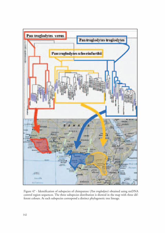
142

Figure 47 - Identification of subspecies of chimpanzee (Pan troglodytes) obtained using mtDNA control region sequences. The three subspecies distribution is showed in the map with three dif-ferent colours. At each subspecies correspond a distinct phylogenetic tree lineage.

143

EXECUTIVE SUMMARY

Randi E., C. Tabarroni e S. Rimondi (eds.), 2002 - Forensic genetics and the Washington Convention - CITES. Quad. Cons. Natura, 12, Min. Ambiente - Ist. Naz. Fauna Selvatica.

CITES (Convention on International Trade in Endangered Species of Wild Fauna and Flora), is an international agreement which aims at regulating the trade of plants and animals. It is based on the principle that control over the sustainable trade of fauna and flora and their products, constitutes a conservation measure of the wild populations, above all if the concept of sustainable use of living species, forms the basis of international and national legislation. In fact, the correct application of the CITES means that the dynamics of threatened species and populations subject to trade is constantly controlled. CITES works by authoring the issue of import and export permits of living specimens and their products that are among the protected species listed in Appendices I and II. The species in Appendix I are afforded total protection, and trade in specimens of these species is only permitted under exceptional circumstances. Trade of species listed in Appendix II is possible though must be closely controlled. CITES also regulates the detention and trade of fauna and flora repro-duced in captivity and then possibly used for travelling collections or exhibitions. In these cases, CITES permits are issued only when there is proof that these specimens were born and bred in captivity. The EC Commission Regulation No. 1808/2001, regarding the protection of wild fauna and flora through trade regulations establishes that the Management Authorities of the State can avail themselves of genetic testing to determine the origin and the degree of kinship of plants and animals detained and reproduced in captivity. As a consequence of these norms, the Management Authority can issue export permits for commercial purposes of specimens listed in Appendix I reproduced in captivity, only after certification that the specimens in question where actually born in captivity.Forensic genetics is going through a period of rapid progress thanks to the develop-ment of DNA molecular testing methodologies that have reached levels of precision, repeatability and reliability that were unthinkable until recently. The concept of DNA fingerprinting has rapidly become part of everyday speech. Molecular method-ologies have an elevated capacity of identification (every individual, except for iden-tical twins, has a unique genetic profile, that differs from any other individual). The results of laboratory tests can be interpreted in the context of population genet-ics and the theory of probability. In this manner the results of laboratory tests can be expressed in a quantitative manner (probabilistically) and evaluated through sta-tistical analysis. The principal aim of forensic genetic testing is to verify the hypoth-esis that a specific DNA fingerprinting is univocally associated to a particular indi-vidual, or that the DNA fingerprinting of an offspring is derived from the DNA

144

fingerprinting of the two putative parents. The DNA testing methods permit the identification of every individual present in a population and the reconstruction of the degree of relationship within a family unit. The results of DNA tests provide information that can be used as evidence during legal proceedings in law courts. Forensic genetic procedures must guarantee high quality results, that must be evalu-ated accurately and be comprehensible also to those who are not geneticists by pro-fession. Forensic genetic testing is used to provide the competent authorities with objective information that can assist them in making decisions and resolving legal disputes. The methods used in molecular testing which allow the reconstruction of DNA fin-gerprinting are based on observations of the presence of very complex and variable DNA segment arrangements within genomes that are associated exclusively to each individual. The structure of DNA fingerprinting is caused by genetic mutations of the genes that are, almost always, well identified. The variability of DNA finger-printing is rigorously analysed using models of population genetics and statistic pro-cedures. The use of molecular genetics in forensic science is based on strong biological and statistical data. DNA fingerprinting is widely used in forensic genetics as well as in criminology, and is applied in decisions regarding paternity, identification of animal and plant species and individuals, poaching and trade of living specimens and their products. DNA fingerprinting testing can considerably reduce the level of subjectivity that is inherent in all identification procedures, as long as it is carried out and evaluated correctly. It is opportune to limit the definition of DNA finger-printing to those methods of molecular testing that permit the identification of sam-ples. These methods include: “DNA fingerprinting” recognition of typical multi-loci, achieved by means of multi-locus probes; multiple single locus (each one consisting of a variable number of tandem repeats); “DNA fingerprinting” recognition, attained by means of specific single locus probes; PCR analysis of micro-satellite loci (short tandem repeats). Independently from which method is used, the pattern of DNA segments identified in each sample results in an individual genetic arrangement sample-specific.At the INFS (National Institute for Wild Fauna) Genetic Laboratory, in concord-ance with the Ministry of the Environment, Nature Conservation Department, forensic genetic testing is currently underway in application of the CITES. The test-ing that is being carried out is principally for CITES certification of species born in captivity, and regard numerous bird and mammal species.

145

REFERENCES

BALDING D. J. and R. A. NICHOLS, 1994 - DNA profile match probability calcu-lation. Forensic Sci. Int., 64: 125-140.

EVETT I. W. and B. S. WEIR, 1998 - Interpreting DNA evidence. Sinauer, Sun-derland, MA.

NRC - NATIONAL RESEARCH COUNCIL, 1966 - The Evaluation of Forensic DNA Evidence. http://bob.nap.edu/html/DNA/

JEFFREYS A. J., V. WILSON and S. L. THEIN, 1985 - Hypervariable “minisatellite” regions in human DNA. Nature, 314: 67-73.

PRITCHARD J. K., M. STEPHENS and P. J. DONNELLY, 2000 - Inference of popu-lation structure using multilocus genotype data. Genetics, 155: 945-959.

SOUTHERN E. M., 1975 - Detection of specific sequences among DNA fragments separated by gel electrophoresis. Journal of Molecular Biology, 98: 503-517.

Finito di stampare nel mese di maggio 2003dalla Tipolitografia F.G. Savignano s/Panaro - Modena