PROTODRIVE: SIMULATION OF ELECTRIC VEHICLE POWERTRAINS

NSF Summer Undergraduate Fellowship in Sensor Technologies

Stephanie Diaz (Electrical & Computer Engineering) – Binghamton University

Advisor: Dr. Rahul Mangharam

Summer 2012

ABSTRACT

Electric vehicles are a promising alternative to vehicles powered by fossil fuels due to their

cleaner energy emission, but current limitations in battery technology are preventing electric

vehicles from burgeoning in the mass consumer market. Therefore, simulating and prototyping

various power trains become paramount for finding different energy efficient models. A portable

power train platform, known as Protodrive, is here to provide a stage in between pure software

simulation and full-scale hardware simulation. This platform allows energy to transfer between

the vehicle power train and the load power train through the use of regenerative braking.

Protodrive is also able to accept a plethora of drive cycles and trajectories to help determine the

forces acting on the vehicle. Through the use of mathematical models of these forces, the

platform is capable of applying the proper load on the vehicle power train to determine the power

consumption. Additionally, introduction of a super capacitor to the vehicle power train model

allows for the analysis of various charging schemes to better manage the power consumption.

The resulting simulated drive data can be viewed in real time through an intuitive web

application that will allow users to enter drive cycles and define trajectories using Google Maps.

The platform data can then be validated by comparing it with actual vehicle drive data.

2

Table of Contents

1. INTRODUCTION .....................................................................................................................3

2. BACKGROUND .......................................................................................................................4

2.1 Electric Vehicles Today .................................................................................................4

2.1.1 Types of Electric Vehicles ...........................................................................4

2.1.2 Consumer Acceptance .................................................................................4

2.1.3 Charging and Regenerative Braking ............................................................4

2.2 Super capacitors in Electric Vehicles ............................................................................5

2.3 Overview of Protodrive..................................................................................................5

3. DRIVE CYCLES ON PROTODRIVE ......................................................................................7

3.1 Understanding the Vehicle Model .................................................................................7

3.2 Using MATLAB for Drive Cycle Simulations ............................................................10

3.2.1 Initial MATLAB Setup ..............................................................................11

3.2.2 Creating and Using Trajectories ................................................................11

3.2.3 Simulating Drive Cycles ............................................................................12

4. HARDWARE ..........................................................................................................................15

4.1 Initial Hardware Setup .................................................................................................15

4.2 Hardware Modifications ..............................................................................................16

4.2.1 Motors and Power Supply ..........................................................................16

4.2.2 Current Sensing ..........................................................................................16

4.2.3 Current Flow ..............................................................................................16

5. CONTROLS ............................................................................................................................18

5.1 Naïve Charging Scheme ..............................................................................................18

5.2 Prescient Charging Scheme .........................................................................................19

6. WEB APPLICATION .............................................................................................................20

6.1 Using the Google Maps API ........................................................................................20

6.2 Future Goals .................................................................................................................20

6.2.1 Energy Efficient Routes .............................................................................20

7. DISCUSSION & CONCLUSION ...........................................................................................21

8. RECOMMENDATIONS .........................................................................................................21

9. ACKNOWLEDGEMENTS .....................................................................................................21

10. REFERENCES ........................................................................................................................22

11. APPENDIX ..............................................................................................................................23

3

1. INTRODUCTION

On July 29, 2011, the Obama Administration announced a plan aimed to increase fuel

economy, decrease oil dependence, and reduce pollution. Model year 2016 vehicles are to

have an average fuel efficiency of 35.5 mpg, and model year 2025 vehicles are to have an

average of 54.5 mpg, cutting greenhouse gas emissions by more than 6 billion metric tons

[1]. To help fulfill the administration's goals, thirteen major automakers have agreed to

actively pursue the research and development of electric vehicles [1].

Electric vehicles provide an alternative to vehicles powered by fossil fuels, leading to a

dramatic decrease in dependence on gasoline. However, limitations such as low energy

density, high costs, and long battery recharging time prevent mass consumer acceptance [2].

There are various ways to optimize the efficiency of electric vehicles. For example, the

powertrain system and fuel control could be managed to reach an optimal range. The electric

vehicle powertrain can be modeled using a battery, motor, motor controller, and gearbox.

The mLAB at the University of Pennsylvania has developed a small scale electric vehicle

prototyping platform known as Protodrive [2]. The Protodrive provides a step in between

software simulation and full-scale prototyping. The most important aspect is that the

Protodrive is a physical hardware system that implements a small scale powertrain capable of

fitting on a desktop. It will be able to simulate certain power optimization algorithms while

capturing most hardware problems.

This paper will focus on the development of a method to accurately model vehicles on

Protodrive, as well as the implementation of various charging schemes to better distribute

power consumption among batteries and super capacitors.

4

2. BACKGROUND

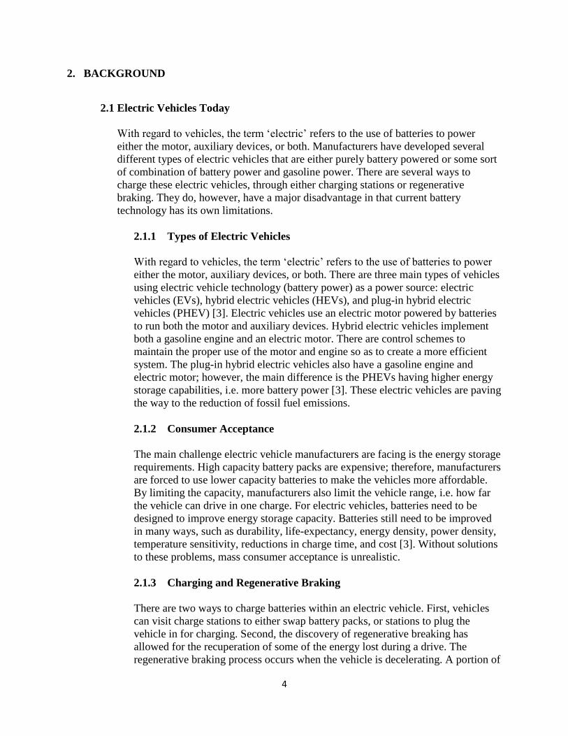
2.1 Electric Vehicles Today

With regard to vehicles, the term ‘electric’ refers to the use of batteries to power

either the motor, auxiliary devices, or both. Manufacturers have developed several

different types of electric vehicles that are either purely battery powered or some sort

of combination of battery power and gasoline power. There are several ways to

charge these electric vehicles, through either charging stations or regenerative

braking. They do, however, have a major disadvantage in that current battery

technology has its own limitations.

2.1.1 Types of Electric Vehicles

With regard to vehicles, the term ‘electric’ refers to the use of batteries to power

either the motor, auxiliary devices, or both. There are three main types of vehicles

using electric vehicle technology (battery power) as a power source: electric

vehicles (EVs), hybrid electric vehicles (HEVs), and plug-in hybrid electric

vehicles (PHEV) [3]. Electric vehicles use an electric motor powered by batteries

to run both the motor and auxiliary devices. Hybrid electric vehicles implement

both a gasoline engine and an electric motor. There are control schemes to

maintain the proper use of the motor and engine so as to create a more efficient

system. The plug-in hybrid electric vehicles also have a gasoline engine and

electric motor; however, the main difference is the PHEVs having higher energy

storage capabilities, i.e. more battery power [3]. These electric vehicles are paving

the way to the reduction of fossil fuel emissions.

2.1.2 Consumer Acceptance

The main challenge electric vehicle manufacturers are facing is the energy storage

requirements. High capacity battery packs are expensive; therefore, manufacturers

are forced to use lower capacity batteries to make the vehicles more affordable.

By limiting the capacity, manufacturers also limit the vehicle range, i.e. how far

the vehicle can drive in one charge. For electric vehicles, batteries need to be

designed to improve energy storage capacity. Batteries still need to be improved

in many ways, such as durability, life-expectancy, energy density, power density,

temperature sensitivity, reductions in charge time, and cost [3]. Without solutions

to these problems, mass consumer acceptance is unrealistic.

2.1.3 Charging and Regenerative Braking

There are two ways to charge batteries within an electric vehicle. First, vehicles

can visit charge stations to either swap battery packs, or stations to plug the

vehicle in for charging. Second, the discovery of regenerative breaking has

allowed for the recuperation of some of the energy lost during a drive. The

regenerative braking process occurs when the vehicle is decelerating. A portion of

5

the kinetic energy stored in the vehicle’s translating mass is regained and can be

stored in a battery or capacitor. This is generally done by allowing the traction

motor to act as a generator, giving the proper braking torque to the wheels and

recharging the traction batteries [4]. This recovered energy can then be used for

either the motor or auxiliary devices.

1.1 Super capacitors in Electric Vehicles for Buffering

A driving cycle can place different types of strains on the vehicle. These strains

include traffic, especially stop-and-go traffic, sudden acceleration due to driver

behavior, and varying terrains. Because of these electric loads on the vehicle, the

current surges traveling in and out of the battery tend to generate extensive heat inside

the battery. This leads to increased battery internal resistance, which results in lower

efficiency and eventually premature failure. This poses a problem when regenerative

braking occurs because the process produces a sudden increase in the amount of

current entering the batteries. These current spikes can lead to the degradation of the

batteries [5]-[7]. A super capacitor, however, has a high power density, meaning it

can rapidly charge and discharge. Therefore, it is effective ad a buffer for the batteries

[8].

2.2 Overview of Protodrive

Fig. 1. [2] Protodrive platform

6

Protodrive was previously developed by University of Pennsylvania students William

Price and Anthony Botelho [2]. Most powertrain simulations are currently done

strictly on software and then created on a full-scale prototype vehicle [2]. This

process can be quite costly and very time consuming since it requires putting together

so many components. However, Protodrive is a small, portable, and easily modifiable.

The platform consists of two models: the vehicle model, and load model. Both of

these models are controlled by a microcontroller. The vehicle model is comprised of a

brushed DC motor, motor controller with regenerative braking capabilities, lithium

ion cells used in the Tesla Roadster, and a super capacitor. There is currently a relay

to switch between the super capacitor and battery pack, giving the user control over

when to charge and discharge the super capacitor. This model represents a vehicle’s

energy consumption [2].

The load model is also comprised of the same lithium ion cells, a brushed DC motor,

and a motor controller with regenerative braking. The two motors (vehicle and load)

are rigidly coupled together. This way, the load motor can act against the vehicle

motor to simulate the proper load in a real-world situation [2]. There will be a more

detailed explanation of how these loads are modeled and simulated in Section 3.

7

3. DRIVE CYCLES ON PROTODRIVE

The first step in being able to model the vehicle and the load acting upon it is finding a

proper mathematical model for all the forces both driving the motor and acting against the

motor. These models are then used in MATLAB to create the proper input voltage for each

motor.

3.1 Understanding the Vehicle Model

The platform is comprised of the

load and the vehicle model. They

are rigidly coupled as shown in

Fig. 2. According to W. Price and

A. Botelho, the total force acting

on the vehicle at any moment in

time is split up into several

different forces [2]:

Where,

Total tractive force at the wheels

Force due to acceleration

Force due to gravity

Force due to aerodynamic drag

Force due to rolling resistance of the tires

These individual forces can be calculated by using vehicle specific parameters:

( )

( )

Where,

Total mass acting on the wheels

Acceleration of the vehicle

Mass of the vehicle

Gravity

Angle of inclination of the

vehicle

Frontal area of the vehicle

Coefficient of drag

Velocity of the vehicle

Coefficient of rolling resistance

The total mass of the vehicle represents the combination of the vehicle mass and

the mass added due to the inertia of all the rotating components. In general, the

moment of inertia can be converted into mass using:

Vehicle Motor Load MotorCoupler

Fig. 2. Vehicle and load motor coupling

8

Where,

Torque

Moment of inertia

Angular acceleration

Wheel radius

Force

Mass

Acceleration

Using this equation it is possible to find the mass due to the moment of inertia:

Where,

Mass due to moment of inertia

Mass due to moment of inertia of wheels

Mass due to moment of inertia of gearbox and motors

Radius of wheels

Moment of inertia of wheels

Gearbox ratio

Moment of inertia of gearbox and motors

The total mass of the vehicle can now be written as:

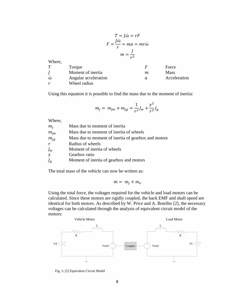
Using the total force, the voltages required for the vehicle and load motors can be

calculated. Since these motors are rigidly coupled, the back EMF and shaft speed are

identical for both motors. As described by W. Price and A. Botelho [2], the necessary

voltages can be calculated through the analysis of equivalent circuit model of the

motors:

Vl

L

R

Coupler

R

VdVemf

L

Vemf

Vehicle Motor Load Motor

Fig. 3. [2] Equivalent Circuit Model

9

Through this model, the vehicle motor voltage and load motor voltage are described

by:

Where,

Vehicle motor voltage

Resistance

Vehicle motor current

Inductance

Back EMF

Speed constant

Load motor voltage

Load motor current

Angular velocity

Torque

Current

Torque constant

Using the mechanical coupling equation, they described the torque as:

Where,

Moment of inertia of both motors and a coupler

Vehicle motor torque

Load motor torque

Torque to overcome friction

The electrical and mechanical equations can be combined to calculate the proper

motor voltages (the inductance has been set to zero to make it simpler):

( )

Where,

Torque scaling between actual vehicle and Protodrive

Necessary torque

10

Necessary angular velocity

Necessary angular acceleration

These equations can now be used to run a simulation on the platform. They are used

in MATLAB, which communicates with an mbed NXP LPC1768 microcontroller for

PWM control. The function, calculate_Vd_Vl, outputs and using a set of vehicle

and motor parameters, as well as the angle of inclination, velocity, and acceleration of

the vehicle.

3.2 Using MATLAB for Drive Cycle Simulations

Vehicle drive cycles contain information about how quickly a vehicle is traveling

along a path. This information provides the velocity and acceleration required for

voltage calculations. Several drive cycles were used for testing the platform. The first

set of drive cycles was created in MATLAB for testing various trajectories, as well as

how the platform reacts to a certain range of velocities.

The second set of data was the federal drive cycle obtained from the U.S.

Environmental Protection Agency as shown in Fig. 4.

Fig. 4. [9] EPA Urban Dynamometer Driving Schedule

This drive cycle demonstrates a vehicle’s stop-and-go characteristics as well as high

speed characteristics. This is important because stop-and-go drive cycles exemplify a

vehicle’s ability to regenerate some of its energy through braking. However, there is

no GPS data for obtaining a trajectory for the vehicle.

The third set of drive cycles was obtained from the Charge Car project at Carnegie

Mellon University. There are numerous trips available with GPS and velocity data.

This was used to simulate a drive cycle involving both the trajectory data, mainly

used to calculate the angle of inclination, and the velocity data. This combination

provides all the necessary data to run a full simulation that accounts for all the forces

acting on the vehicle.

11

3.2.1 Initial MATLAB Setup

The initial MATLAB GUI contained two different trajectories with

predefined duty cycles (voltages) for each motor. The first trajectory is a

trapezoidal path showing how the motors would react to uphill, straight,

and downhill paths. This was used mainly for debugging purposes since

the current drawn for the vehicle motor can be easily predicted and then

tested on this path. The second trajectory is a sinusoidal path showing how

the motors would react to multiple hills. This is mainly used to

demonstrate the regenerative capabilities of the system. However, it is

necessary for the platform to demonstrate an array of diverse paths, as

well as real-world routes.

3.2.2 Creating and Using Trajectories

The first set of trajectories was created using two dimensional paths for

simplicity. Various trajectories could be created using piecewise linear

equations; however, having a discontinuous path is nonrealistic since real

driving paths have smooth transitions. Therefore, Bezier curve principles

were used to provide continuous paths. The Bezier function created in

MATLAB would accept an array of points for the path to follow, the total

horizontal distance of the path, and the sampling rate with respect to the x-

axis. With this, a set of fundamental paths was created: hill, multiple hills,

straight, and steep downhill.

These trajectories were then passed through a second function called,

response_to_path. This takes in the x and y coordinates of the path, as well

as the length of the vehicle (l_v), and the drive cycle. The most important

information necessary from the trajectory is the slope of the vehicle at

each instant in time. Therefore, a series of steps need to be taken in order

to extract this data successfully. First, the length of the path at each x-

coordinate is calculated. This information is then used to calculate the

slope between every l_v in order to find the angle of inclination of the

vehicle with respect to the x-axis. Second, the vehicles acceleration and

position are calculated with respect to time. This is done using the drive

cycle entered as an input to the function. Third, the angle of inclination

with respect to time is found using the position of the vehicle. All of this

information is entered into the calculate_Vd_Vl function to obtain the

required voltages at each time instant.

Since this was initially done using only two dimensional trajectories, the

next objective was to create three dimensional trajectories and a way to

analyze them for calculating the voltages. This was done easily by creating

a Bezier function that would create three dimensional paths by accepting

an array of yz-coordinates (z being in the upward direction) for the path to

12

follow. The paths created with this function can then be analyzed by an

improved response_to_path function. This function is different in that the

calculations for the angle of inclination are done using vector calculus.

With these functions, drive cycles on trajectories can be simulated on

Protodrive.

3.2.3 Simulating Drive Cycles

The duty cycles obtained from the voltage calculations have to be sent to

the microcontroller, which communicates these values to the motor

controllers. This is done using the RPC interface library for MATLAB that

is provided by mbed, the microcontroller manufacturer. MATLAB

variables can be easily linked to variables used in the microcontroller

code. The microcontroller then scales the duty cycles appropriately to stay

within the operating range of the motors. However, high velocity drive

cycles require high voltages for the motors. Since these voltages were out

of range, it is necessary to scale the velocity down. This will then be

accounted for when scaling back up to the energy consumption of an

actual vehicle.

Speed and current data was retrieved from sensors for a drive cycle on a

hill, as shown in Fig. 5. The velocity remained constant at 7 m/s to test

whether the platform was responding to the hill.

Fig. 5. Trajectory for the vehicle to follow

0 100 200 300 400 500 600 700 8000

5

10

15

20

25

30

35

40

45Path for Vehicle

Distance (meters)

Heig

ht

(mete

rs)

13

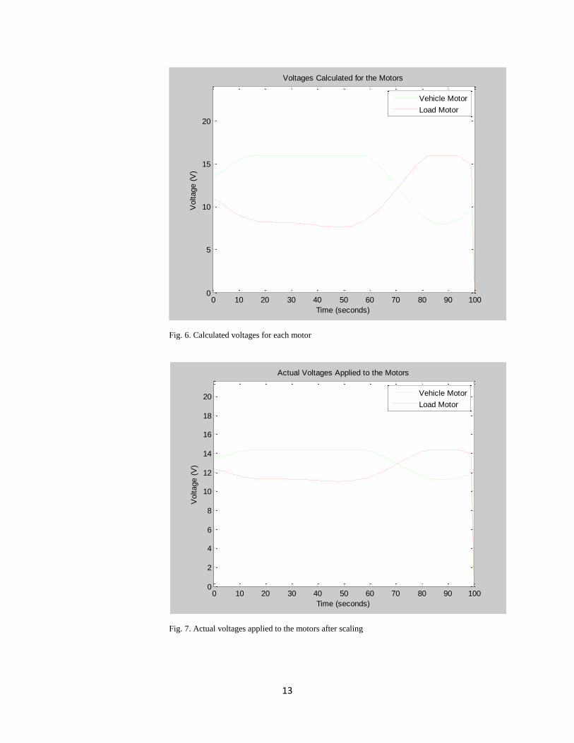
Fig. 6. Calculated voltages for each motor

Fig. 7. Actual voltages applied to the motors after scaling

0 10 20 30 40 50 60 70 80 90 1000

5

10

15

20

Voltages Calculated for the Motors

Time (seconds)

Voltage (

V)

Vehicle Motor

Load Motor

0 10 20 30 40 50 60 70 80 90 1000

2

4

6

8

10

12

14

16

18

20

Actual Voltages Applied to the Motors

Time (seconds)

Voltage (

V)

Vehicle Motor

Load Motor

14

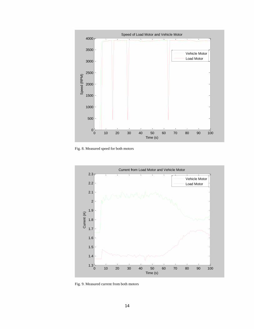
Fig. 8. Measured speed for both motors

Fig. 9. Measured current from both motors

0 10 20 30 40 50 60 70 80 90 1000

500

1000

1500

2000

2500

3000

3500

4000Speed of Load Motor and Vehicle Motor

Time (s)

Speed (

RP

M)

Vehicle Motor

Load Motor

0 10 20 30 40 50 60 70 80 90 1001.3

1.4

1.5

1.6

1.7

1.8

1.9

2

2.1

2.2

2.3

Current from Load Motor and Vehicle Motor

Time (s)

Curr

ent

(A)

Vehicle Motor

Load Motor

15

As shown in Fig. 6, the voltage for the load motor exceeds the voltage for

the vehicle motor as the vehicle drives downhill. This represents

regeneration because the load motor will actually be spinning the vehicle

motor, generating current on the vehicle side. Fig. 7 is a scaled version of

the calculated voltages. This scaling was done to place the calculated

voltages within the range of the motors’ voltage requirements. Fig. 8 and

Fig. 9 show the measured speed and current readings. The speed is fairly

constant due to the constant velocity drive cycle entered. There are minor

fluctuations due to the motor’s direction changes. The current readings are

directly correlated with the power consumption on each battery pack. The

current readings demonstrate the vehicle is using more current as it goes

uphill and less current as it travels downhill.

Fig. 10. MATLAB GUI simulating the hill trajectory

4. HARDWARE

4.1 Initial Hardware Setup

Protodrive consists of two brushed DC motors that are rigidly coupled so they put a

load on each other. These motors are controlled by two SyRen 10A motor controllers

that are capable of regenerative braking. The motor controllers are set in analog

mode, where it accepts an analog signal for PWM control and accepts a signal for

changing directions. These signals are controlled by the microcontroller. The two

motors and motor controller are powered by 14.8V lithium ion batteries, the same

16

ones used in the Tesla Roadster vehicles. The power on the vehicle motor can be

supplied by either a super capacitor or the batteries. The switching is done by a relay

controlled by the microcontroller.

4.2 Hardware Modifications

4.2.1 Motors and Power Supply

The battery packs had initially provided a total of 7.4V, limiting the speed

of the motors to about 300 RPM. This became an issue since high velocity

drive-cycles are impossible to simulate without any extreme velocity

scaling. However, the motors are capable of reaching 6800 RPM. The

power supply was then doubled to 14.8V for better simulations.

4.2.2 Current Sensing

Two changes have been made to the current sensing set up. First, the

current sensor initially was not sensitive enough for the system. Current

readings from an ammeter indicate current varying from about -0.4A to

2A. Therefore, a sensor with a smaller reading range replaced the original

current sensor. Second, current sensing was initially done solely on the

vehicle motor side, in between the vehicle battery pack and motor

controller. However, it is necessary to analyze the current on the load

motor as well. An additional current sensor has been placed in between the

load battery pack and motor controller.

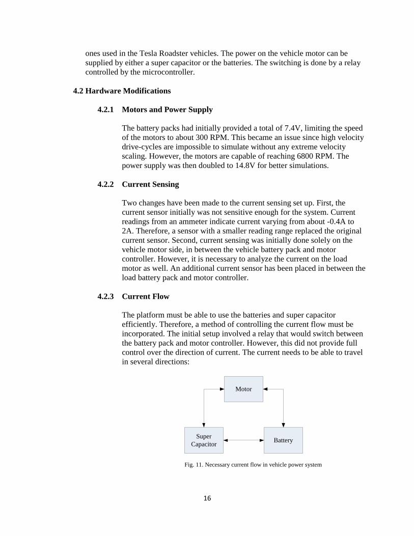
4.2.3 Current Flow

The platform must be able to use the batteries and super capacitor

efficiently. Therefore, a method of controlling the current flow must be

incorporated. The initial setup involved a relay that would switch between

the battery pack and motor controller. However, this did not provide full

control over the direction of current. The current needs to be able to travel

in several directions:

Motor

BatterySuper

Capacitor

Fig. 11. Necessary current flow in vehicle power system

17

As seen in Fig. 10, there must be bidirectional current flow between each

component in the vehicle power model. This application will allow

various charging schemes to be implemented in the system. Therefore, a

new circuit is being introduced to help control the current flow.

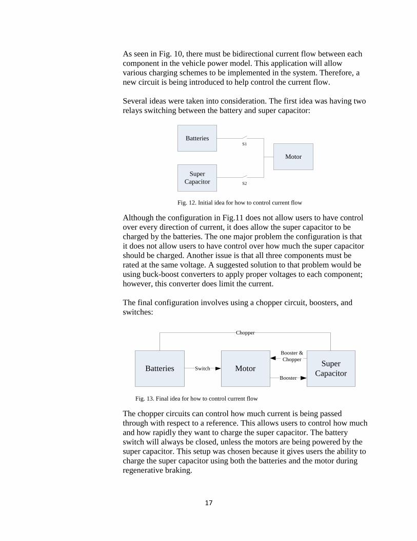
Several ideas were taken into consideration. The first idea was having two

relays switching between the battery and super capacitor:

Batteries

Motor

S1

S2

Super

Capacitor

Fig. 12. Initial idea for how to control current flow

Although the configuration in Fig.11 does not allow users to have control

over every direction of current, it does allow the super capacitor to be

charged by the batteries. The one major problem the configuration is that

it does not allow users to have control over how much the super capacitor

should be charged. Another issue is that all three components must be

rated at the same voltage. A suggested solution to that problem would be

using buck-boost converters to apply proper voltages to each component;

however, this converter does limit the current.

The final configuration involves using a chopper circuit, boosters, and

switches:

Batteries MotorSuper

Capacitor

Booster &

Chopper

Booster

Switch

Chopper

Fig. 13. Final idea for how to control current flow

The chopper circuits can control how much current is being passed

through with respect to a reference. This allows users to control how much

and how rapidly they want to charge the super capacitor. The battery

switch will always be closed, unless the motors are being powered by the

super capacitor. This setup was chosen because it gives users the ability to

charge the super capacitor using both the batteries and the motor during

regenerative braking.

18

5. CONTROLS

There are several control policies that need to be implemented on the platform. The controls

aspect involves finding the most energy efficient charging scheme given the path and drive

cycles. This is done by switching between the super capacitor and batteries for different

conditions. For example, going uphill puts a strain on low power batteries, but is fine for a

high power super capacitor. During these times, the super capacitor should be used to

increase battery life.

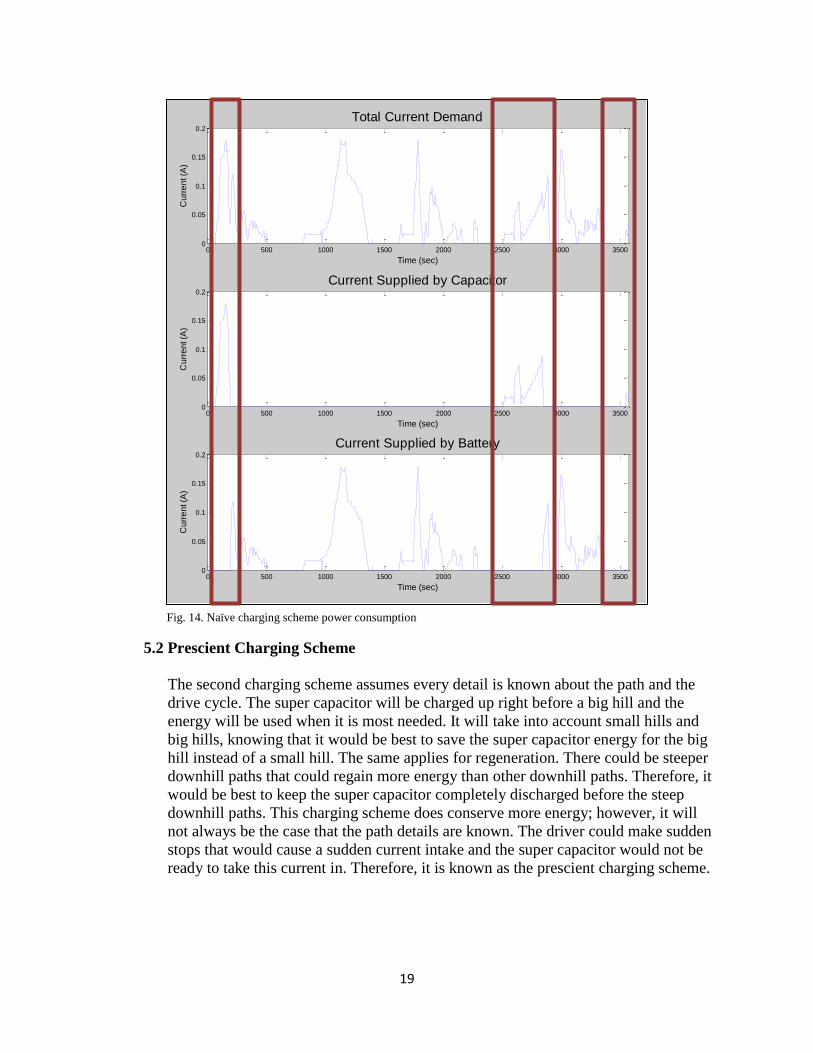
5.1 Naïve Charging Scheme

The first charging scheme is simple but not the most energy efficient. The super

capacitor is charged by regeneration from the motors whenever it occurs. This is good

for the batteries because the sharp current intake can harm and degrade them. As soon

as the capacitor is finished charging, the microcontroller checks whether the voltage

is within the operating range of the motor. If the super capacitor has the proper

voltage, the energy will be used to power the motors. Otherwise, the batteries will

continue running the motors. As seen in Fig. 13, about an 8% improvement can be

seen in the battery current consumption. The problem with this charging scheme is

that the energy in the super capacitor is not being used during crucial moments, for

example going uphill. Therefore, it is known as the naïve charging scheme.

19

5.2 Prescient Charging Scheme

The second charging scheme assumes every detail is known about the path and the

drive cycle. The super capacitor will be charged up right before a big hill and the

energy will be used when it is most needed. It will take into account small hills and

big hills, knowing that it would be best to save the super capacitor energy for the big

hill instead of a small hill. The same applies for regeneration. There could be steeper

downhill paths that could regain more energy than other downhill paths. Therefore, it

would be best to keep the super capacitor completely discharged before the steep

downhill paths. This charging scheme does conserve more energy; however, it will

not always be the case that the path details are known. The driver could make sudden

stops that would cause a sudden current intake and the super capacitor would not be

ready to take this current in. Therefore, it is known as the prescient charging scheme.

0 500 1000 1500 2000 2500 3000 35000

0.05

0.1

0.15

0.2

Total Current Demand

Time (sec)

Cu

rre

nt (A

)

0 500 1000 1500 2000 2500 3000 35000

0.05

0.1

0.15

0.2

Current Supplied by Capacitor

Time (sec)

Cu

rre

nt (A

)

0 500 1000 1500 2000 2500 3000 35000

0.05

0.1

0.15

0.2

Current Supplied by Battery

Time (sec)

Cu

rre

nt (A

)

Fig. 14. Naïve charging scheme power consumption

20

6. WEB APPLICATION

Users should be able to easily choose paths for simulations, as well as enter in a drive cycle

and vehicle parameters. Although this can be done in MATLAB, not all users will have

access to MATLAB. Therefore, a web application is being developed to provide a more

intuitive user interface. The front end of the application is created using Javascript and

HTML in conjunction with the Google Maps API. The MATLAB functions will all be

deployed as an ASP.NET component to be stored onto a server. These functions will be

accessed using ASP.NET and called in the application using Visual Basic C#.

6.1 Using the Google Maps API

The Google Maps Javacript API V3 was used mainly to retrieve map data including

longitude, latitude, and elevation. The user will enter in an origin and a destination,

and the application will display directions for the fastest route. This route will then be

used as an input to for finding the longitude, latitude, and elevation along the path.

The one disadvantage is that each request will only output 512 samples. For long

routes, such as from New York, NY to Philadelphia, PA, this sample size is too small.

Therefore, a quick solution would be to split the route up into n number of paths and

send a request for each path. This will result in a total of 512*n samples. This data

then can be used as inputs to the deployed MATLAB functions.

6.2 Future Goals

The web application will be interactive and allow users to put in any path and drive

cycle. It will communicate with Protodrive and run these drive cycles in real-time,

displaying a video feed of the platform in action. There will be multiple graphs

updating the speed, current, and elevation data as the vehicle drives along the path.

6.2.1 Energy Efficient Routes

Once data has been collected for different drive cycles, there will be an

option under directions for the most energy efficient path. This will route

the vehicle through trajectories that will elongate the battery life of electric

vehicles. For example, the routing algorithm will find paths without steep

uphill paths. This will be done once Protodrive has energy consumption

data along segments throughout a region.

21

7. DISCUSSION & CONCLUSION

The purpose of this project was to simulate various drive cycles and trajectories using

different control policies. The drive cycles were communicated to the platform using an

mbed microcontroller that translates the duty cycles calculated in MATLAB. The trajectories

created in MATLAB started with simple paths involving hills. These were used for testing to

see if the proposed voltages for the motors matched the theoretical values. As shown in Figs.

6-7, the voltages for each motor changed as expected for varying slopes. Some of these drive

cycles were initially difficult to simulate due to having high velocities. However, once the

power supply was doubled, the motors were able to run at higher speeds and were consuming

more current as expected. There were some issues with sensing current since the current

sensor already in place was for reading much higher current values. This was soon replaced

with sensors that could read currents at around 0.5A to 1A with sufficient sensitivity. There

is still future work that needs to be done to perfect Protodrive and have it efficiently run

using many different control policies.

8. RECOMMENDATIONS

Protodrive could be linked with another project being worked on in the lab called Groovenet.

Groovenet is a vehicle simulation program that includes map data. Instead of using the

Google Maps API, the platform could be used in conjunction with Groovenet. Groovenet

provides the user with more freedom when choosing drive cycles and trajectories. Traffic

information such as stop signals and speed limits can be easily added to help with the energy

efficient routing algorithm. This platform can also be validated for different vehicles. By

collecting drive data from different electric vehicles, the platform data can be compared to

see how well it is modeling the vehicle.

9. ACKNOWLEDGEMENTS

I would like to thank Professor Rahul Mangharam for his continuous support, guidance, and

advice throughout the program. Many thanks also to Yash Pant and Harsh Jain for their hours

of work and contribution to this project, as well as their support and guidance during the

program. I would like to thank the mLab for all of their help. Also, I would like to thank Dr.

Jan Van der Spiegel and the rest of the SUNFEST committee for organizing this program and

making it possible. Finally, I would like to thank the National Science Foundation for their

support and financial contribution that provided her with this great opportunity.

22

10. REFERENCES

[1] Obama Administration, "Driving Efficiency: Cutting Costs for Families at the Pump and

Slashing Dependence on Oil." 2012.

[2] W. Price and A. Botelho, "Protodrive: Rapid prototyping and simulation for EV

powertrains," University of Pennsylvania, 2012.

[3] L. Fulton, J. Ward, P. Taylor and T. Kerr, "Technology roadmap: Electric and plug-in

hybrid electric vehicles," International Energy Agency, 2011.

[4] J. Guo, J. Wang and B. Cao, "Regenerative braking strategy for electric vehicles," in 2009

IEEE Intelligent Vehicles Symposium, June 3, 2009 - June 5, 2009, pp. 864-868.

[5] S. Pay and Y. Baghzouz, "Effectiveness of battery-super capacitor combination in electric

vehicles," in 2003 IEEE Bologna PowerTech Conference, June 23, 2003 - June 26, 2003, pp.

728-733.

[6] P. T. Moseley, "High-rate, valve-regulated lead-acid batteries-suitable for hybrid electric

vehicles?" in Electrochemical Energy Conversion and Storage Systems for Mobile

Application, 1999, pp. 237-42.

[7] Electrosource, Battery Handbook, Horizon C2M Batteries, 1999.

[8] A. Styler, G. Podnar, P. Dille, M. Duescher, C. Bartley and I. Nourbakhsh, "Active

management of a heterogeneous energy store for electric vehicles," in 2011 IEEE Forum on

Integrated and Sustainable Transportation Systems (FISTS 2011), 2011, pp. 20-5.

[9] U.S. Environmental Protection Agency, "Federal Test Procedure Revisions,"

http://www.epa.gov/oms/sftp.htm

23

11. APPENDIX

Trajectories and Drive Cycles:

Steep Downhill with Constant Velocity:

0 50 100 150 200 250 300 350 400 450 5000

5

10

15

20

25

30

35

40

45

50Path for Vehicle

Distance (meters)

Heig

ht

(mete

rs)

0 10 20 30 40 50 60 70 80 90 100-0.5

0

0.5

1

1.5Direction Required for the Motors

Time (seconds)

Duty

Cylc

e

Vehicle Motor

Load Motor

0 10 20 30 40 50 60 70 80 90 1000

0.5

1Duty Cycle Required for the Motors

Time (seconds)

Duty

Cylc

e

Vehicle Motor

Load Motor

24

Multi-Hill with Constant Velocity:

0 200 400 600 800 1000 1200 1400 1600 1800 20000

20

40

60

80

100

Path for Vehicle

Distance (meters)

Heig

ht

(mete

rs)

0 50 100 150 200 250 300-0.5

0

0.5

1

1.5Direction Required for the Motors

Time (seconds)

Duty

Cylc

e

Vehicle Motor

Load Motor

0 50 100 150 200 250 3000

0.5

1Duty Cycle Required for the Motors

Time (seconds)

Duty

Cylc

e

Vehicle Motor

Load Motor

25

Straight Path with EPA Urban Dynamometer Driving Cycle:

0 100 200 300 400 500 600 700 800 900 10000

2

4

6

8

10

12

14Path for Vehicle

Distance (meters)

Heig

ht

(mete

rs)

0 200 400 600 800 1000 1200-0.5

0

0.5

1

1.5Direction Required for the Motors

Time (seconds)

Duty

Cylc

e

0 200 400 600 800 1000 12000

0.5

1Duty Cycle Required for the Motors

Time (seconds)

Duty

Cylc

e

Vehicle Motor

Load Motor

Vehicle Motor

Load Motor

26

Seattle Trip using Charge Car Project GPS Data:

0

2000

4000

6000

0

1000

2000

3000

4000

0

50

100

150

x (meters)

Path for Vehicle

y (meters)

z (

mete

rs)

0 1000 2000 3000 4000 5000 6000 7000 8000 9000

0

20

40

60

80

100

120

140

Elevation vs. Distance

Distance (meters)

Ele

vation (

mete

rs)

27

0 100 200 300 400 500 600 700 800 900-0.5

0

0.5

1

1.5Direction Required for the Motors

Time (seconds)

Duty

Cylc

e

Vehicle Motor

Load Motor

0 100 200 300 400 500 600 700 800 9000

0.5

1Duty Cycle Required for the Motors

Time (seconds)

Duty

Cylc

e

Vehicle Motor

Load Motor

28

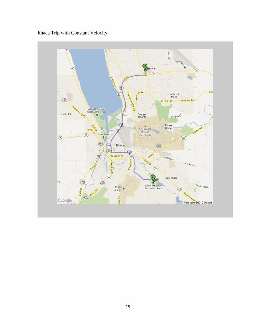
Ithaca Trip with Constant Velocity:

29

0 1000 2000 3000 4000 5000 60000

2000

4000

150

200

250

300

350

400

450

500

Path for Vehicle

x (meters)

y (meters)

z (

mete

rs)

0 1000 2000 3000 4000 5000 6000 7000 8000 9000

100

150

200

250

300

350

400

Elevation vs. Distance

Distance (meters)

Ele

vation (

mete

rs)

30

0 100 200 300 400 500 600 700 800 900-0.5

0

0.5

1

1.5Direction Required for the Motors

Time (seconds)

Duty

Cylc

e

Vehicle Motor

Load Motor

0 100 200 300 400 500 600 700 800 9000

0.5

1Duty Cycle Required for the Motors

Time (seconds)

Duty

Cylc

e

Vehicle Motor

Load Motor

31

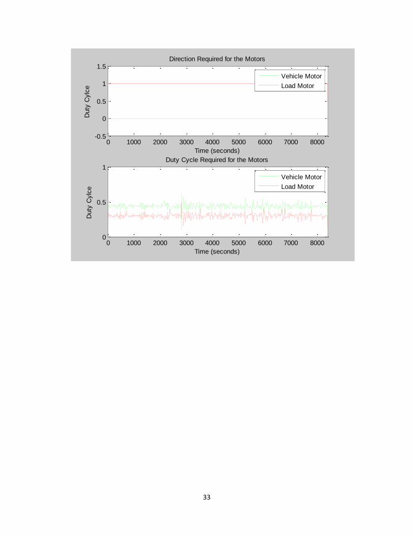
New York, NY to Philadelphia, PA Trip with Constant Velocity:

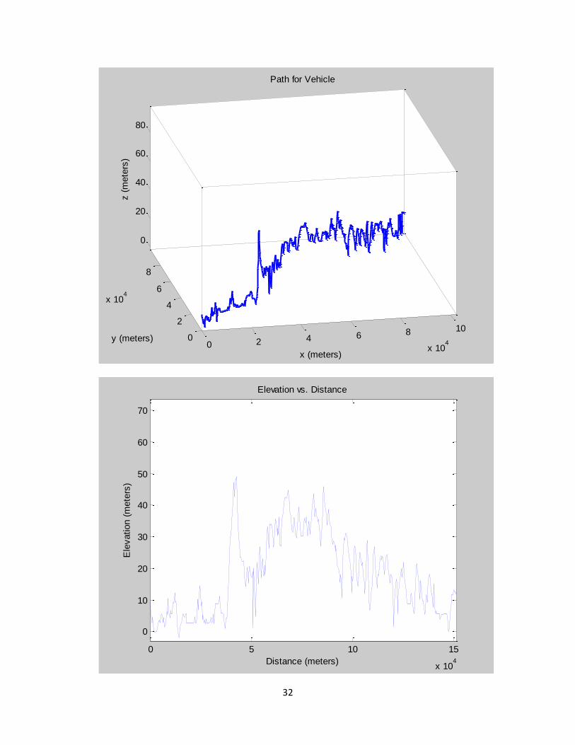
32

0 2 4 6 8 10

x 104

0

2

4

6

8

x 104

0

20

40

60

80

Path for Vehicle

x (meters)

y (meters)

z (

mete

rs)

0 5 10 15

x 104

0

10

20

30

40

50

60

70

Elevation vs. Distance

Distance (meters)

Ele

vation (

mete

rs)

33

0 1000 2000 3000 4000 5000 6000 7000 8000-0.5

0

0.5

1

1.5Direction Required for the Motors

Time (seconds)

Duty

Cylc

e

Vehicle Motor

Load Motor

0 1000 2000 3000 4000 5000 6000 7000 80000

0.5

1Duty Cycle Required for the Motors

Time (seconds)

Duty

Cylc

e

Vehicle Motor

Load Motor