influence of driving patterns on life cycle cost and ... · of hybrid and plug-in electric vehicle...

Energy Policy ∎ (∎∎∎∎) ∎∎∎–∎∎∎

Contents lists available at SciVerse ScienceDirect

Energy Policy

0301-42http://d

n CorrE-m

jmichale1 Te

Pleasin el

journal homepage: www.elsevier.com/locate/enpol

Influence of driving patterns on life cycle cost and emissionsof hybrid and plug-in electric vehicle powertrains

Orkun Karabasoglu a,1, Jeremy Michalek a,b,n

a Mechanical Engineering, Carnegie Mellon University, 5000 Forbes Avenue, Pittsburgh, PA 15213, USAb Engineering and Public Policy, Carnegie Mellon University, Scaife Hall 324, 5000 Forbes Avenue, Pittsburgh, PA 15213, USA

H I G H L I G H T S

� Electrified vehicle life cycle emissions and cost depend on driving conditions.
� GHGs can triple in NYC conditions vs. highway (HWFET), cost +30%.� Under NYC conditions hybrid and plug-in vehicles cut GHGs up to 60%, cost 20%.� Under HWFET conditions they offer few GHG reductions at higher costs.� Federal tests for window labels and CAFE standards favor some technologies over others.
a r t i c l e i n f o

Article history:Received 30 January 2012Accepted 25 March 2013

Keywords:Driving conditionsLife cycle assessmentPlug-in hybrid electric vehicles

15/$ - see front matter & 2013 Elsevier Ltd. Ax.doi.org/10.1016/j.enpol.2013.03.047

esponding author. Tel.: +1 412 268 3765; fax:ail addresses: [email protected] (O. [email protected] (J. Michalek).l.: +1 412 268 3606; fax: +1 412 268 3348.

e cite this article as: Karabasoglu, O.,ectric vehicle powertrains. Energy Po

a b s t r a c t

We compare the potential of hybrid, extended-range plug-in hybrid, and battery electric vehicles toreduce lifetime cost and life cycle greenhouse gas emissions under various scenarios and simulateddriving conditions. We find that driving conditions affect economic and environmental benefits ofelectrified vehicles substantially: Under the urban NYC driving cycle, hybrid and plug-in vehicles can cutlife cycle emissions by 60% and reduce costs up to 20% relative to conventional vehicles (CVs). In contrast,under highway test conditions (HWFET) electrified vehicles offer marginal emissions reductions athigher costs. NYC conditions with frequent stops triple life cycle emissions and increase costs ofconventional vehicles by 30%, while aggressive driving (US06) reduces the all-electric range of plug-invehicles by up to 45% compared to milder test cycles (like HWFET). Vehicle window stickers, fueleconomy standards, and life cycle studies using average lab-test vehicle efficiency estimates are thereforeincomplete: (1) driver heterogeneity matters, and efforts to encourage adoption of hybrid and plug-invehicles will have greater impact if targeted to urban drivers vs. highway drivers; and (2) electrifiedvehicles perform better on some drive cycles than others, so non-representative tests can bias consumerperception and regulation of alternative technologies. We discuss policy implications.

& 2013 Elsevier Ltd. All rights reserved.

1. Introduction

The Obama Administration's New Energy for America agendaset a target of achieving 1 million plug-in vehicles on U.S. roads by2015 (Obama and Biden, 2009–04–11). Plug-in vehicles, includingplug-in hybrid electric vehicles (PHEVs) and battery electricvehicles (BEVs), may play a key role in cutting national gasolineconsumption, addressing global warming, and reducing depen-dency on foreign oil in the transportation sector. Plug-in vehiclesoperate partly or entirely on inexpensive electricity that can be

ll rights reserved.

+1 412 268 3348.asoglu),

Michalek, J., Influence of drlicy (2013), http://dx.doi.or

potentially obtained from local, renewable, and less carbon-intensive energy sources than gasoline (Bradley and Frank, 2009;Samaras and Meisterling, 2008). Based on the 2009 NationalHousehold Travel Survey (NHTS) (U.S. Department ofTransportation, 2009), approximately 60% of U.S. passenger vehi-cles that drove on the day surveyed traveled less than 30 mi, adistance that could be powered entirely by electricity using plug-in vehicles. Thus, plug-in vehicles have the potential to offset asubstantial amount of gasoline consumption even when chargedonly once per day.

The fuel economy and emissions of vehicles depend on the waythey are driven, including daily driving distance (Shiau et al., 2010;Traut et al., 2012; Kelly et al., 2012; Neubauer et al., 2012, 2013;Raykin et al., 2012a,b) and driving conditions. Official fuel economyratings are based on standard test driving conditions – called

iving patterns on life cycle cost and emissions of hybrid and plug-g/10.1016/j.enpol.2013.03.047i

www.elsevier.com/locate/enpol

www.elsevier.com/locate/enpol

http://dx.doi.org/10.1016/j.enpol.2013.03.047



mailto:[email protected]

mailto:[email protected]





O. Karabasoglu, J. Michalek / Energy Policy ∎ (∎∎∎∎) ∎∎∎–∎∎∎2

a driving cycle – but real-world driving patterns can vary sub-stantially from standard test cycles (Patil et al., 2009; Berry, 2010),leading real-world costs and emissions to deviate from thoseestimated on window stickers or in life cycle studies. In theliterature, vehicle life cycle assessment and design optimizationstudies are typically conducted using efficiency estimates fromfederal test cycles, with results that favor certain powertrains overothers. In this paper, we investigate variation in life cycle cost andemission benefits of hybrid and plug-in vehicles under a range ofdriving conditions with a sensitivity analysis to critical factors suchas gasoline prices, vehicle costs and electricity grid mix. Specifi-cally, we compare conventional vehicle (CV), hybrid electricvehicle (HEV), PHEV, and BEV powertrain technologies and iden-tify changes in all-electric range (AER), vehicle efficiency, andbattery life, under a variety of driving patterns to determine themost cost effective and lowest GHG-intensive powertrains. Thenwe discuss the energy policy implications of our findings con-sidering multiple scenarios related to market, vehicle technology,and electricity grid mix.

1.1. Electrified vehicle powertrain alternatives

Electrified powertrains include HEVs, which use a small batteryto improve gasoline fuel efficiency but do not plug in; PHEVs,which use both gasoline and electricity; and BEVs, which use onlyelectricity and not gasoline. All three powertrains share anadvantage over conventional vehicles: each is capable of regen-erative braking. When a conventional car brakes, the vehicle'skinetic energy dissipates mostly as heat. In contrast, an electrifiedvehicle with regenerative braking capability can capture and storesome of this energy in its battery. In addition, HEVs and PHEVs areable to manage engine operating conditions to improve efficiency,turn off the gasoline engine at idle, and make use of higherefficiency, lower torque thermodynamic cycles.

Fig. 1 demonstrates the relationship between the battery andthe different operation modes of plug-in vehicles. For safety,reliability, and longevity reasons, electrified vehicle powertrainsuse only a certain portion of the full energy capacity of its battery,limited by the specified maximum and minimum battery state ofcharge (SOC) values. Operation of PHEVs can be categorized intotwo modes as seen in Fig. 1: charge-depleting (CD) mode refers tothe phase where the SOC is above the target SOC and the vehiclereceives some or all of its net propulsion energy from the battery

Fig. 1. Operation modes of a PHEV (figu

Please cite this article as: Karabasoglu, O., Michalek, J., Influence of drin electric vehicle powertrains. Energy Policy (2013), http://dx.doi.or

pack. Once the battery is depleted to a target SOC, the vehicleswitches to charge-sustaining (CS) mode, in which gasoline is usedto provide all net propulsion energy and the electrical system isused only as momentary storage to improve fuel economy, similarto a grid-independent HEV. Some PHEVs operate CD-mode usingonly electrical energy. Such a configuration, referred to as an all-electric control strategy or an extended-range electric vehicle(EREV), enables short trips to be driven without any gasolineconsumption but requires electric motor and battery designs thatcan deliver the vehicle's maximum power demands. Other PHEVdesigns operate CD-mode using a mixture of gasoline and elec-trical energy. Such a configuration, referred to as a blended controlstrategy, does not eliminate gasoline consumption even for shorttrips, but power demands on electrical components are lower,allowing smaller, cheaper components to be used. We focus onEREV PHEVs, since the performance of blended-operation PHEVsvaries substantially with control strategy parameters (Tulpuleet al., 2009; Sciarretta et al., 2004; Sciarretta and Guzzella, 2007;Moura et al., 2011). Operation of a BEV is similar to that of an EREVPHEV in CD mode, and operation of an HEV is similar to that of aPHEV in CS mode.

Hybridization can be based on 3 specific powertrain architec-tures: (1) series, where the engine turns the generator whichgenerates electricity to be used by the electric motor to turn thewheels; (2) parallel, which is capable of transmitting torque to thewheels from two different energy sources; and (3) split, whichuses a planetary gear device to operate both in series and parallel.For greatest flexibility, we adopt the split powertrain for HEV andPHEV designs, as shown in Fig. 2, which is currently used in theToyota Prius HEV and PHEV.

Current gasoline spark-ignition engine technology can typicallyprovide 20% efficiency under urban driving with a maximum of35% under the most optimal conditions (Heywood, 2006). Theselow efficiencies suffer even more under real world driving condi-tions, where closer to 10% of the chemical energy of each gallon ofgasoline acts to turn the wheels. The rest of the energy is lost inthe form of heat and sound. With the help of a planetary gear-based power-split device, hybridization allows the engine tooperate near its most efficient torque and speed values whileproviding excess power to recharge the battery or drawingremaining power needs from the motor. In this way large amountsof fuel might be saved, depending on the drive cycle. The motor issupplied with the electric energy from the battery, which is

re adapted from Shiau et al. (2010).





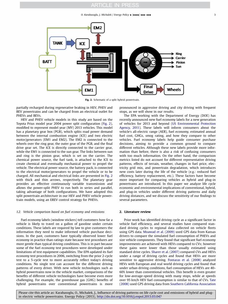
Fig. 2. Schematic of a split hybrid powertrain.

O. Karabasoglu, J. Michalek / Energy Policy ∎ (∎∎∎∎) ∎∎∎–∎∎∎ 3

partially recharged during regenerative braking in HEV, PHEV andBEV powertrains and can be charged from an electrical outlet forPHEVs and BEVs.

HEV and PHEV vehicle models in this study are based on theToyota Prius model year 2004 power split configuration (Fig. 2),modified to represent model year (MY) 2013 vehicles. This modelhas a planetary gear box (PGB), which splits road power demandbetween the internal combustion engine (ICE) and two electricmotor/generators (EM1 and EM2). The EM2 is connected to thewheels over the ring gear, the outer gear of the PGB, and the finaldrive gear set. The ICE is directly connected to the carrier gear,while the EM1 is connected to the sun gear. The links between sunand ring is the pinion gear, which is set on the carrier. Thechemical power source, the fuel tank, is attached to the ICE tocreate chemical and eventually mechanical power to propel thevehicle. The electrical power source, the battery pack, is connectedto the electrical motor/generators to propel the vehicle or to becharged. All mechanical and electrical links are presented in Fig. 2with thick and thin arrows, respectively. The planetary gearprovides an effective continuously variable transmission andallows the power-split PHEV to run both in series and parallel,taking advantage of both configurations. We have adopted thissplit powertrain architecture in our HEV and PHEV vehicle power-train models, using an EREV control strategy for PHEVs.

1.2. Vehicle comparison based on fuel economy and emissions

Fuel economy labels (window stickers) tell customers how far avehicle is likely to travel on a gallon of gasoline under certainconditions. These labels are required by law to give customers theinformation they need to make informed vehicle purchase deci-sions. In the past, customers have typically observed lower fueleconomy in practice than ratings state because test procedures aremore gentle than typical driving conditions. This is in part becausesome of the fuel economy test procedures were developed underlimitations of test equipment capabilities. The EPA updated its fueleconomy test procedures in 2006, switching from the prior 2-cycletest to a 5-cycle test to more accurately reflect today's drivingconditions. No single test can account for the different drivingpatterns of every driver. With new vehicle technologies such ashybrid powertrains now in the vehicle market, comparisons of thebenefits of different vehicle technologies have become even morechallenging. For example, the greenhouse gas (GHG) benefits ofhybrid powertrains over conventional powertrains is more


pronounced in aggressive driving and city driving with frequentstops, as we will show in our results.

The EPA working with the Department of Energy (DOE) hasrecently announced new fuel economy labels for a new generationof vehicles for 2013 and beyond (US Environmental ProtectionAgency, 2011). These labels will inform consumers about thevehicle's all-electric range (AER), fuel economy, estimated annualfuel cost, GHGs, smog rating, and how they compare to othervehicles. Fuel economy labels help guide consumer purchasedecisions, aiming to provide a common ground to comparedifferent vehicles. Although these new labels provide more infor-mation than before, there is also a risk of confusing consumerswith too much information. On the other hand, the comparisonmetrics listed do not account for different representative drivingpatterns, effects of terrain, weather, changes in fuel price, elec-tricity grid mix, and powertrain degradation, which introducesnew costs later during the life of the vehicle (e.g.: reduced fuelefficiency, battery replacement, etc.). These factors have becomemore important for comparing vehicles as hybrid and plug-inpowertrains are introduced. In this paper we analyze life cycleeconomic and environmental implications of conventional, hybrid,and plug-in vehicles under different driving patterns and dailydriving distances, and we discuss the sensitivity of our findings toseveral parameters.

2. Literature review

Prior work has identified driving cycle as a significant factor invehicle fuel efficiency, and several studies have compared stan-dard driving cycles to regional data collected on vehicle fleetsusing GPS data. Moawad et al. (2009) used GPS data from Kansasdrivers to compare the simulated fuel consumption of PHEVs andsize vehicle components. They found that significant fuel economyimprovements are achieved with HEVs compared to CVs; howeverthese gains were lower than those usually estimated usingstandard drive cycles. Sharer et al. (2007) compared CVs and HEVsunder a range of driving cycles and found that HEVs are moresensitive to aggressive driving. Fontaras et al. (2008) analyzedHEVs with European and real world driving cycles and found thatunder urban driving conditions, fuel consumption of HEVs are 40–60% lower than conventional vehicles. This benefit is even greaterfor low-average-speed driving with many stops, while at speedsover 95 km/h HEV fuel consumption is similar to that of CVs. Tate(2008) used GPS driving data from Southern California Association






of Governments (2003), which consists of 621 samples, to studyPHEV performance. The associated power and speed values of thedriving samples are found to be higher than those associated withthe UDDS driving cycle. The study also compares average energyconsumption per unit distance to that of UDDS and HWFET drivecycles and finds that 94% of vehicles function at higher energyconsumption under real-world driving conditions than they dounder UDDS and HWFET cycles. A 2001 report (Energy andEnvironmental Analysis, Inc December, 2001) states that impactof aggressive driving in city conditions varies greatly depending onthe type of vehicle: Powerful vehicles are robust, but low powervehicles show 6% reduction in efficiency compared to standarddrive cycles. However in highway conditions, characterized byhigh speeds, impact of aggressive driving was much higher: 33%penalty for the average car, and 28% for the powerful car. Berry andHeywood (Berry, 2010) analyzed the effect of driving patterns onthe fuel economy of CVs and found that the sensitivity of vehiclefuel economy to aggressive driving is a function of how wheelwork and efficiency vary with driving patterns. Whitefoot et al.(2010) optimized HEVs under different driving cycles for minimalfuel consumption, finding that vehicles designed for one drivingcycle show significantly lower performance on other drive cycles.Patil et al. (2010) optimized a series PHEV for naturalistic drivecycles and showed that the higher energy demands of real worldcycles require larger batteries to meet AER targets. The requiredoptimal battery size changed nonlinearly with desired AER. Fellahet al. (2009) found that if batteries of PHEVs are sized for the UDDScycle, only 22% of 363 trips from Kansas City can be driven in allelectric mode due to power limitations.

Despite the fact that standard cycles are not representative ofreal driving patterns, some of them can span a wide range. Patilet al. (2009) investigated the impact of real world driving cycleson PHEV component sizing using GPS data from southeasternMichigan. Simulations using the GPS driving data indicate thatabout 90% of the trips in the data are higher fuel-consuming permile than the UDDS and HWFET standard cycles, while about 90%of the trips are lower fuel-consuming per mile than the US06cycle. Similarly after examining the Southern California regionaltravel data (Southern California Association of Governments,2003), Tate (2008) found that the vast majority of the energydemanded by the drive cycles of the dataset is bounded by theenergy levels required by US06, a reasonable upper limit, andUDDS, a fair lower limit. Thus both studies agree that UDDS andUS06 appear to provide reasonable bounds to characterize theeffect of driving cycle variation over a population of drivers forconventional vehicles. The authors also emphasize the need forlarger electrical components when real world driving is consid-ered. All of these prior driving cycle studies focus on vehicleperformance and efficiency but do not assess the full lifetime costand life cycle implications of different powertrain technologies.

Life cycle assessment studies have shown that vehicle electri-fication has the potential to reduce GHGs; however, potentialbenefits depend on the source of electricity used to charge thevehicle. In 2009, the U.S. grid mix consisted of 45% coal, 23%natural gas, 20% nuclear, 7% hydroelectric, 4% other renewable, 1%petroleum, and 0.6% other (Administration, U.S.E.I. Annual EnergyReview, 2009). Lipman and Delucchi (2010) provide a review ofstudies. Weber et al. (2010) show that determining regional gridmix is nontrivial, and dispatch studies such as Sioshansi andDenholm (2009) highlight that the mix associated with marginaldemand for electricity varies widely depending on charge timing.Samaras and Meisterling (2008) find that under a high carbon-intensity electricity generation scenario life cycle GHGs of PHEVsare 9–18% higher than HEVs, while GHGs are30–47% lower under a low-carbon scenario. The Electric PowerResearch Institute (EPRI) together with the National Resources


Defense Council (NRDC) (Elgowainy et al., 2009) analyzed the GHGimpacts of PHEVs over the 2010 to 2050 timeframe for severalscenarios including different levels of CO2 intensity in the elec-tricity sector and fleet penetration of PHEVs. Some of the assump-tions include projections of vehicle time-of-day charging, plantdispatch, plant retirement and construction, and public policy.Each of the EPRI scenarios showed significant GHG reductions, andPHEV adoption reduces petroleum consumption significantly.Argonne's well-to-wheels report (Argonne National Laboratory,2009) states that PHEVs charging from the US average grid-mixproduce 20% to 25% lower GHGs than CVs but 10% to 20% higherGHGs than gasoline HEVs. They suggest that to receive significantreductions in emissions, PHEVs and BEVs must recharge from agrid-mix which consists of largely non-fossil sources. According totheir study, electric range decreases with real world driving.Michalek et al. (2011) estimate the economic value of life cycleoil consumption and air emissions externalities from conventional,hybrid and plug-in vehicles, finding that HEVs and PHEVs withsmaller battery packs provide the greatest benefits per dollarspent. Hawkins et al. (2012) provide a life cycle inventory of CVsand BEVs and find that BEVs decrease global warming potential by10–24% under a European grid mix.

A few studies have examined the role of driving patterns on lifecycle implications, primarily assessing the importance of variationin driving distance. Shiau et al., (2010) constructed an optimizationmodel to find the optimal allocation of CVs, HEVs, and PHEVs todrivers based on driving distance to minimize life cycle GHGemissions, finding that optimal allocation based on distance is asecond order effect. Traut et al. (2012) extended Shiau's study toinclude BEVs and workplace charging infrastructure whileaccounting for day to day driving variability. They identify gasolineand battery prices needed for plug-in vehicles to enter the cost-minimizing solution. Neubauer et al. (2012, 2013) investigated thesensitivity of PHEV and BEV to driving distance and chargingpatterns, accounting for factors such as battery degradation andthe need for a backup vehicle for BEVs when taking long trips.They find that changing the drive pattern can increase the PHEV-to-CV cost ratio by a factor of up to 1.6, and the cost of backupvehicles for BEVs can be substantial. Kelly et al. (2012) used NHTSdata and examined the effects of charging location, time, rate, andbattery size. Finally, Raykin et al. (2012a,b) analyzed the effect ofdriving patterns on tank-to-wheel energy use of PHEVs, using anestimated relationship between driving distance and drive cyclebased on a travel demand model and vehicle driving simulation.They find that PHEVs result in greater GHG reductions relative toCVs in city rather than highway conditions.

With the exception of Raykin et al. (2012a,b), those studies thatinvestigate variations in drive cycle focus on the effects onperformance or efficiency without examining the larger system(e.g.: full life cycle), and those studies that investigate life cycleimplications of electrified vehicles either ignore variation indriving conditions or confine scope to examining variation indriving distance and charge timing. Raykin et al. examine bothdrive cycle and distance in a study of the greater Toronto area,concluding that both matter in estimating life cycle implications.We build on this finding by examining a range of drive cycles anddistribution of driving distances for the United States and estimat-ing effects on life cycle emissions, gasoline consumption, lifetimeownership cost, battery degradation, and AER for CVs, HEVs, BEVs,and PHEVs of varying battery capacity.

3. Methodology

We use the Powertrain Systems Analysis Toolkit (PSAT) SP1Version 6.2, developed by Argonne National Laboratory (2008), to






model conventional, hybrid, plug-in hybrid, and battery electricvehicles with identical body characteristics, comparable controlstrategies, and comparable performance characteristics, and wesimulate each vehicle over a range of drive cycles to comparevehicle efficiency and life cycle implications (Fig. 3). We accountfor battery degradation, different daily driving distances anddifferent scenarios for costs, vehicle technology and electricitygrid. In this section we explain each model and their interactionsin detail. First, we discuss the choice and characteristics of drivingcycles and travel patterns. Then we describe engineering, batterydegradation, cost, and environmental models.

3.1. Driving cycles

Efforts to assess and improve the fuel economy and emissionsof vehicles are typically not conducted under real-world driving,since multiple noise factors such as various driving patterns, trafficconditions, weather, and terrain might affect the results. Instead,tests are done in a laboratory under controlled and repeatableconditions so that even small fuel economy improvements are notlost due to the noise in the environment. This enables designers,analysts and regulators to compare different vehicle designs toeach other on a common basis. A chassis dynamometer is thedevice used to simulate driving in laboratory conditions: thewheels are placed on rollers that simulate the road load bymatching the inertia of the car so that the propulsion system ofthe vehicle needs to work to rotate the wheels at a certainreference speeds. The speed reference used in this test is takenfrom a given drive cycle (test cycle) in the form of a series of targetvehicle speed values over time. During the test a driver tries tomatch the vehicle's speed to the reference speed at each momentin time using visual feedback by a computer screen. An emissionanalyzer is connected to the exhaust pipe of the vehicle to trackemissions and estimate fuel consumption. Different driving cycles

Bat

tery

siz

e

EngineeMode

GHG Mo

Cost M

PerformaAnalys

Range ofdrive cycles

Reference drive cycle (EPA combined 2008+)

e

PeInitial vehicle designs

Battery Degradation

Model

National Driving Data (NHTS)

Final Vehicle Designs

Range of Scenarios for Market,

Technology and Grid

Energy processed

Fig. 3. Framework of vehicle life cycle benefit


used during this test result in different performance demands andthus different fuel consumption and emissions. The performanceof some powertrain designs may be more sensitive to driving cyclethan others. EPA has been using standard driving cycles (FTP andHWFET) to report the fuel consumption and emissions of vehicles.When these test cycles were designed, chassis dynamometertechnology was not capable of simulating high acceleration anddeceleration (Austin et al., 1993), and the test cycles wereconstrained to conditions less aggressive than observed in prac-tice. Also because traffic patterns have changed since the 1960sand 1970s, when the FTP and HWFET drive cycles were created,they may fail to represent typical driving conditions today. In2006, EPA announced a new method to measure fuel economybased on a five-cycle testing method in an effort to better reflectreal world performance. According to this method, vehicles aretested on aggressive (US06), air conditioning on (SC03) and coldweather (Cold FTP) drive cycles in addition to city (FTP) andhighway (HWFET). Characteristics of these drive cycles are given inTable 1 (Berry, 2010). Weighted combinations of these test resultsare used to calculate the city and the highway fuel economy values(EPA, 2006). Alternatively, automakers could use unadjusted FTPand HWFET test results in some regression equations to approx-imate the 5-cycle city and highway fuel economies, with somerestrictions during 2008–2010. EPA (2006):

Five� cycle city fuel economy

¼ 10:003259þ ð1:1805Þ=ðFTP fuel economyÞ ð1Þ

Five� cycle highway fuel economy

¼ 10:001376þ ð1:3466Þ=ðHWFET fuel economyÞ ð2Þ

EPA combined MPG 2008þ½ �

ring l

del

odel

nce is

Fuel fficiencies

rformance criteria

Lifetime Cost

Itera

tion

GHG

Vehicle component technology

and size

Life Cycle GHGs

comparison for different driving patterns.





Table 2Driving cycle characteristics (Argonne National Laboratory, 2008).

Statistics Units UDDS HWFET US06 NYC LA92

Distance mi 7.45 10.27 8.01 1.17 9.82Max. speed mi/h 56.70 59.90 80.29 27.53 67.20Avg. speed mi/h 19.58 48.28 47.96 7.05 24.61Avg. acceleration m/s2 0.50 0.19 0.67 0.62 0.67Avg. deceleration m/s2 −0.58 −0.22 −0.73 −0.60 −0.75Time at rest (%) % 18.92 0.65 7.5 35.12 16.31Stop freq. (#/mi) mi�1 2.28 0.10 0.62 15.38 1.63

0%

100%

200%

300%

400%

500%

600%

700%

Ave. speed Ave. acc Stop freq.

UD

DS

Driving cycle characteristics

UDDS

HWFET

NYC

US06

LA92

Fig. 4. Driving cycle characteristics.


¼ 10:43=ð5−cycle city MPGÞ þ 0:57=ð5−cycle highway MPGÞ

ð3ÞFor MY2011 and beyond, the 5-cycle fuel economy method is

required to be used; however, if the five-cycle city and highwayfuel economy results of a test vehicle group are within 4% and 5%of the regression line, respectively, then the automaker is per-mitted to continue using the regression estimates. These regres-sion equations may be optimistic or pessimistic estimates ofmeasured 5-cycle fuel economy, depending on vehicle and power-train design. The equations were developed for gasoline vehicles;however, we also apply them to estimate reductions in electricalefficiency of plug-in vehicles for the 5-cycle fuel economyestimates.

While the new standards offer an improvement in estimatingreal-world fuel economy, test estimates can still differ from real-world driving, favoring certain vehicle designs and powertrainsover others and representing some driver habits and drivingconditions better than others. We can understand the effects ofdifferent driving styles by considering approximate upper andlower bounds on those styles. To evaluate how the relativebenefits of different vehicle technologies change with respect todriving cycles, we examine five different driving cycles plus theEPA combined estimate: (1) the Urban Dynamometer DrivingSchedule (UDDS) represents city driving conditions for light dutyvehicles which are characterized by relatively slow speed. UDDS isalso called LA4, FTP72 and FUDS and is related to the FTP cycle;(2) the Highway Fuel Economy Test (HWFET) which representshighway driving conditions under 60 mph; (3) the US06 cycle is anaggressive driving cycle with high acceleration and high engineloads; (4) the NYC cycle represents low speed urban driving withfrequent stops; (5) the LA92 cycle is an aggressive driving cycle incity conditions; and (6) the combined MPG computed by the EPAby weighting city and highway efficiency. We use regression Eqs.(1)–(3) to adjust fuel and electrical efficiency values of FTP, HWFET,and combined fuel economy. Table 1 and Table 2 summarize thecharacteristics of these driving cycles for comparison, and Fig. 4shows the statistics normalized to unadjusted UDDS, which isadopted by several life cycle and optimization studies in theliterature. We will summarize the adjusted and unadjusted effi-ciencies of vehicles in Table 4.

Patil et al. (2009) find that the US06 is more fuel-consumingthan 90% of real-world GPS cycles collected in southeast Michigan.The NYC cycle is low speed with frequent stops and relatively high

Table 1Characteristics of U.S. certification drive cycles (Berry, 2010).

Drive cycle FTP HWET US06

Description Urban/city Free-flow traffic onhighway

Aggresshighway

Regulatory use(2010)

CAFE & label CAFE & label Label

Data collectionmethod

Instrumented vehicles/specific route

Chase-car/naturalisticdriving

Instrumnaturali

Year of datacollection

1969 Early 1970s 1992

Top speed 90 kph (56 mph) 97 kph (60 mph) 129 kphAvg. velocity 32 kph (20 mph) 77 kph (48 mph) 77 kph (Max. accel. 1.48 m/s2 1.43 m/s2 3.78 m/sDistance 11 mi (17 km) 10 mi (16 km) 8 mi (13Time (min) 31 min 12.5 min 10 minStops 23 None 4Idling time 18% None 7%Engine start Cold Warm WarmLab. temp. 68–86 1F 68–86 1F 68–86 1FAir conditioning Off Off Off


acceleration and deceleration, serving as a reasonable bound onurban driving conditions. LA92 represents somewhat more aggres-sive and higher speed driving in city conditions. A recent study byAymeric et al. (2008) claims that this cycle is closer to real-worlddriving than the standard test cycles, partially due to the fact thatit was designed using data collected in 1992, after dynamometertechnology had improved.

3.2. Distribution of daily distance driven

Daily driving distance is an important factor in estimating thereal benefits of electrified vehicles since EREV PHEVs have thepotential to power daily trips entirely on electricity if the distancebetween charge points is shorter than the AER of the PHEV. If dailydistance driven is longer than the AER, there will be additionalgasoline consumption.

SC03 C-FTP

ive driving on AC on, hot Ambient temp. City, cold Ambient temp.

Label Label

ented vehicles/stic

Instrumented vehicles/naturalistic

Instrumented vehicles/specific route

1992 1969

(80 mph) 88 kph (54 mph) 90 kph (56 mph)48 mph) 35 kph (22 mph) 32 kph (20 mph)2 2.28 m/s2 1.48 m/s2

km) 3.6 mi (5.8 km) 11 mi (18 km)9.9 min 31 min5 2319% 18%Warm Cold95 1F 20 1FOn Off






The second implication of daily driving distance is that vehiclelife depends on use. Typical vehicle life is assumed to be approxi-mately 150,000 mi (EPA, 2005). Daily driving distance determinesthe life of the vehicle and the amount of time over which thepurchase cost is spread, which is important for computing netpresent value of lifetime vehicle ownership.

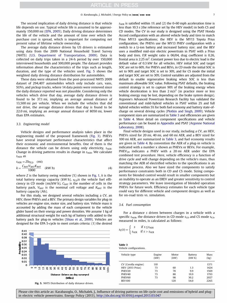
The average daily distance driven by US drivers is estimatedusing data from the 2009 National Household Travel Survey(NHTS) (U.S. Department of Transportation, 2009). Data iscollected on daily trips taken in a 24-h period by over 150,000interviewed households and 300,000 people. The dataset providesinformation about the characteristics of the trips such as length,duration, and the type of the vehicles used. Fig. 5 shows theweighted daily driving distance distribution for automobiles.

These data were obtained from the post-processed NHTS 2009dataset of 294,407 automobiles which only include cars, vans,SUVs, and pickup trucks, where 14 data points were removed sincethe daily distance reported was not plausible. Considering only thevehicles which drive that day, average daily distance driven isfound to be 37.1 mi, implying an average annual distance of13,500 mi per vehicle. When we include the vehicles that didnot drive, the average distance driven that day is found to be22.0 mi, implying an average annual distance of 8050 mi, lowerthan EPA estimates.

3.3. Engineering model

Vehicle designs and performance analysis takes place in theengineering model of the proposed framework (Fig. 3). PHEVshave several important performance characteristics that affecttheir economic and environmental benefits. One of them is thedistance the vehicle can be driven using only electricity, sAER.Change in driving patterns results in change in sAER. We calculatesAER as

sAER ¼ ZkηCD ðmiÞ

k¼ CBATVBATKBAT

1000ðkW hÞ ð4Þ

where Z is the battery swing window (%) shown in Fig. 1, k is thetotal battery energy capacity (kW h), ηCDis the vehicle fuel effi-ciency in CD mode (mi/kW h), CBAT is the number of cells in thebattery pack, VBAT is the nominal cell voltage and KBAT is thebattery capacity (Ah).

For this study, we designed several vehicles including a CV, anHEV, three PHEVs and a BEV. The primary design variables for plug-invehicles are engine size, motor size, and battery size. Vehicle mass isaccounted by adding the mass of each component to the vehicleglider based on their energy and power densities. We assume 1 kg ofadditional structural weight for each kg of battery cells added to thebattery pack for plug-in vehicles (Shiau et al., 2009). Vehicles aredesigned for the EPA 5-cycle to meet certain criteria: (1) the desired

Fig. 5. NHTS Distribution of daily distance driven.


sAER is satisfied within 1% and (2) the 0–60 mph acceleration time isless than 10.3 s (the reference set by the HEV model) in both CS andCD modes. The CV in our study is designed using the PSAT HondaAccord configuration with an altered vehicle body and tires to matchPrius MY13 specifications; the HEV is the MY13 Toyota Priusconfiguration; the PHEVs use the MY13 PHEV configuration with aswitch to a Li-ion battery and increased battery size; and the BEVuses a modified mid-size electric powertrain in PSAT with a Priusbody and tires. F/R weight ratio is 06/04, drag coefficient is 0.26,frontal area is 2.25 m2. Constant power loss due to electric load is thedefault value of 0.3 kW for all vehicles. HEV initial SOC and targetSOC are set to 60%. For PHEVs and BEVs, in CD mode the initial SOC isset to 90% and target SOC is set to 30%, and for CS mode the initialand target SOC are set to 30%. Control variables are adjusted from thedefault to enable regenerative braking when SOC is less thanmaximum allowable SOC value. Following PSAT defaults, the brakingcontrol strategy is set to capture 90% of the braking energy whenvehicle deceleration is less than 2 m/s2 (in practice more or lessbraking energy may be lost, depending on the brake system design).Argonne's Advanced Powertrain Research Facility has validated theconventional and mild-hybrid vehicles in PSAT within 2% and fullhybrid vehicles within 5% for both fuel economy and battery state-of-charge on several driving cycles (Plotkin and Singh, 2009). Vehiclecomponent sizes are summarized in Table 3 and efficiencies are givenin Table 4. More detail on component specifications and vehicleperformance can be found in Appendix and PSAT (Argonne NationalLaboratory, 2008).

Final vehicle designs used in our study, including a CV, an HEV,PHEVs sized for 20 mi, 40 mi, and 60 mi AER, and a BEV sized for100 mi AER, are summarized in Table 3, and fuel economy resultsare given in Table 4. By convention the AER of a plug-in vehicle isindicated with a number x shown as PHEVx or BEVx. For example,PHEV20 indicates a PHEV with a 20 mi AER under the EPAcombined test procedure. Here, vehicle efficiency is a function ofdrive cycle and will change depending on the vehicle's mass, thusmatching the AER of electrified vehicles to the specifications is aniterative process. Also we have sized the components to satisfyperformance constraints both in CD and CS mode. Sizing compo-nents for blended control would result in smaller components butan inability to operate as an EREV and greater sensitivity to controlstrategy parameters. We leave investigation of blended operationPHEVs for future work. Efficiency estimates for each vehicle typecould vary for different vehicle and component designs as well asfor on-road tests vs. simulation.

3.4. Fuel consumption

For a distance s driven between charges in a vehicle with aspecific sAER, the distance driven in CD mode sCD and CS mode sCS,measured in miles, is calculated as follows:

sEðsÞ ¼s if s≤sAER

sAER if s4sAER

(

Table 3Vehicle configurations.

Vehicle type Engine Motor Battery Mass(kW) (kW) (kW h) (kg)

CV (Corolla engine) 110 1371HEV (2013 Prius) 73 60 1.3 1424PHEV20 73 78 9.9 1569PHEV40 73 88 19.9 1793PHEV60 73 98 30.2 2027BEV100 120 54.0 2265





Table 4Efficiency and AER of each vehicle under each driving cycle. The label “2008+” refers to the regression-based adjusted fuel economy calculations used by the EPA between2008 and 2011 and beyond 2011 under some specific conditions (Eqs. (1)–(3)).

Vehicle type UDDS HWFET US06 NYC LA92 FTP EPA city(2008+) EPA highway(2008+) EPA Combined MPG (2008+)

CV mi/gal 32.1 52.8 29.8 16.4 28.9 32.8 25.4 37.2 31.0HEV mi/gal 69.5 59.7 43.9 48.0 54.1 67.8 48.4 41.8 44.4PHEV20

CD eff mi/kW h 6.2 5.7 3.2 4.2 4.2 6.0 3.3 3.6 3.4CD-mpg-eq mpg-eq 207.9 193.0 108.4 142.0 142.2 202.3 110.0 119.7 115.3CS eff mi/gal 69.4 58.6 41.0 45.7 52.3 67.3 48.1 41.1 43.8AER mi 36.8 34.1 19.2 25.1 25.2 35.8 19.5 21.2 20.4

PHEV40CD eff mi/kW h 6.0 5.7 3.2 4.1 4.1 5.8 3.2 3.5 3.4CD-mpg-eq mpg-eq 201.2 192.1 106.9 138.2 138.1 196.2 107.8 119.3 114.0CS eff mi/gal 68.0 58.2 40.2 43.1 50.0 66.0 47.3 40.8 43.4AER mi 71.2 68.0 37.8 48.9 48.9 69.4 38.1 42.2 40.3

PHEV60CD eff mi/kW h 5.7 5.6 3.1 3.8 3.9 5.6 3.1 3.5 3.3CD-mpg-eq mi/kW h 192.2 190.0 104.0 129.6 132.2 188.0 104.8 118.1 112.0CS eff mi/gal 65.8 57.8 39.2 40.3 48.0 64.0 46.1 40.5 42.7AER mi 103.5 102.3 56.0 69.8 71.2 101.2 56.4 63.6 60.3

BEV100CD eff mi/kW h 4.8 5.2 3.4 3.1 4.1 4.8 2.8 3.3 3.1CD-mpg-eq mi/kW h 162.2 176.4 113.5 103.8 136.9 160.9 94.4 111.0 103.2AER mi 155.9 169.6 109.1 99.8 131.6 154.7 90.7 106.7 99.2


sGðsÞ ¼0 if s≤sAER

s−sAER if s4sAER

(ð5Þ

The NHTS-averaged distance driven on electricity sE andaverage distance driven on gasolinesG is given by

sE ¼Z ∞

s ¼ 0sEf SðsÞds

sG ¼Z ∞

s ¼ 0sGf SðsÞds ð6Þ

where fS(s) is the probability distribution function (PDF) ofdistance driven for a randomly selected vehicle on a randomdriving day in the NHTS 2009 data, including those vehicles thatwere not driven on the day surveyed. We discretize this distribu-tion into 1-mi bins for numerical integration.

Average distance driven per day s is given as

s¼Z ∞

s ¼ 0sf SðsÞds ð7Þ

Gasoline consumption gðsÞ, given in gallons, and electricityconsumption eðsÞ, given in kW h, on a day with s miles of driving iscalculated by

gðsÞ ¼ maxð0; s−sAERÞηCS

eðsÞ ¼ minðs; sAERÞηCD

ð8Þ

where ηCS and ηCD values are fuel efficiencies in CD and CS modes,respectively, summarized in Table 4.

The average gasoline g and electricity e consumption in theNHTS data set given as

g¼Z ∞

s ¼ 0gðsÞf SðsÞds

e¼Z ∞

s ¼ 0eðsÞf SðsÞds ð9Þ

Typical vehicle life, sLIFE is assumed to be approximately150,000 mi (EPA, 2005). D is the number of days in the year(365). Vehicle life TVEH(s) in years is given by:

TVEHðsÞ ¼sLIFEDs

ð10Þ


and the NHTS average vehicle life is:

TVEH ¼ sLIFEDs

ð11Þ

3.5. Battery degradation model

We follow Peterson et al. (2010a) and Shiau et al. (2010) inmodeling battery degradation as a function of energy processed,based on data collected from A123 LiFePO4 cells. Energy processedwDRV in kW h while driving a distance s is:

wDRVðsÞ ¼ μCDsE þ μCSsG ð12Þwhere μCD and μCS are the energies processed per mile (kW h/mi)in CD and CS modes, respectively. Energy processed, given inkW h, while charging is:

wCHGðsÞ ¼ sEðηCDηBÞ−1 ð13Þwhere ηB is the battery charging efficiency, assumed to be 95%. Therelative energy capacity fade can be calculated as

rPðsÞ ¼αDRVwDRV þ αCHGwCHG

kð14Þ

where αDRV¼3.46�10−5 and αCHG¼3.46�10−5 are the relativeenergy capacity fade coefficients derived from the data set in(Peterson et al., 2010a). We define battery end of life (EOL) as thepoint when the portion of the remaining energy capacity equalsthe energy within the swing window under the original capacity.The relative energy capacity fade rEOL at the EOL becomes theoriginal total capacity minus swing (rEOL¼1−Z).

The NHTS average computed battery life, given in years, isfound by:

TBAT ¼kð1−ZÞ

ðαDRVðμCDsE þ μCSsGÞ þ αCHGsEðηEηCÞ−1ÞDð15Þ

We assume that the functional battery life in the vehicle θBAT isnever longer than vehicle life:

θBAT ¼minðTBAT; TVEHÞ ð16ÞWe ignore degradation effects for NiMH cells in the HEV

because HEV performance is far less sensitive to capacity fade(effectively an AER of zero); HEV economics are less sensitive topossible battery replacement; and our Li-ion degradation modelpredicts no replacement for the HEV configuration and use





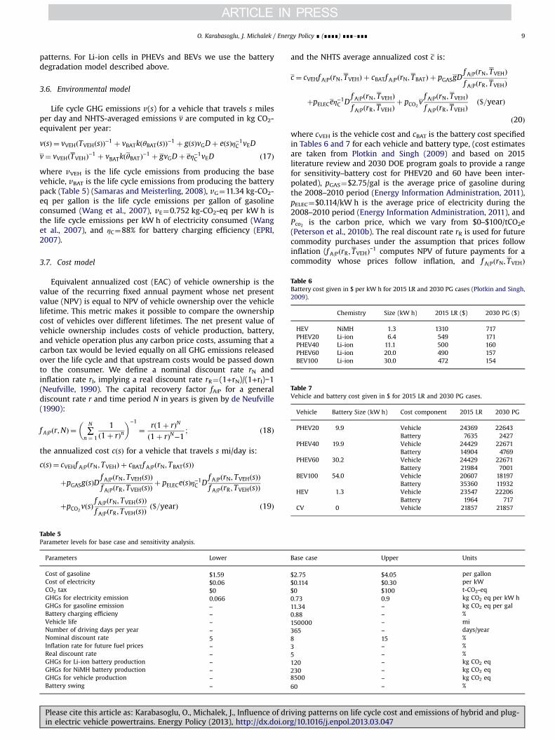
Table 6Battery cost given in $ per kW h for 2015 LR and 2030 PG cases (Plotkin and Singh,2009).

Chemistry Size (kW h) 2015 LR ($) 2030 PG ($)

HEV NiMH 1.3 1310 717PHEV20 Li-ion 6.4 549 171PHEV40 Li-ion 11.1 500 160PHEV60 Li-ion 20.0 490 157BEV100 Li-ion 30.0 472 154

Table 7Vehicle and battery cost given in $ for 2015 LR and 2030 PG cases.

Vehicle Battery Size (kW h) Cost component 2015 LR 2030 PG

PHEV20 9.9 Vehicle 24369 22643Battery 7635 2427



BEV100 54.0 Vehicle 20607 18197Battery 35360 11932

HEV 1.3 Vehicle 23547 22206Battery 1964 717

CV 0 Vehicle 21857 21857


patterns. For Li-ion cells in PHEVs and BEVs we use the batterydegradation model described above.

3.6. Environmental model

Life cycle GHG emissions v(s) for a vehicle that travels s milesper day and NHTS-averaged emissions v are computed in kg CO2-equivalent per year:

vðsÞ ¼ vVEHðTVEHðsÞÞ−1 þ vBATkðθBATðsÞÞ−1 þ gðsÞvGDþ eðsÞη−1C vED

v¼ vVEHðTVEHÞ−1 þ vBATkðθBATÞ−1 þ gvGDþ eη−1C vED ð17Þwhere vVEH is the life cycle emissions from producing the basevehicle, vBAT is the life cycle emissions from producing the batterypack (Table 5) (Samaras and Meisterling, 2008), vG¼11.34 kg-CO2-eq per gallon is the life cycle emissions per gallon of gasolineconsumed (Wang et al., 2007), vE¼0.752 kg-CO2-eq per kW h isthe life cycle emissions per kW h of electricity consumed (Wanget al., 2007), and ηC¼88% for battery charging efficiency (EPRI,2007).

3.7. Cost model

Equivalent annualized cost (EAC) of vehicle ownership is thevalue of the recurring fixed annual payment whose net presentvalue (NPV) is equal to NPV of vehicle ownership over the vehiclelifetime. This metric makes it possible to compare the ownershipcost of vehicles over different lifetimes. The net present value ofvehicle ownership includes costs of vehicle production, battery,and vehicle operation plus any carbon price costs, assuming that acarbon tax would be levied equally on all GHG emissions releasedover the life cycle and that upstream costs would be passed downto the consumer. We define a nominal discount rate rN andinflation rate rI, implying a real discount rate rR¼(1+rN)/(1+rI)−1(Neufville, 1990). The capital recovery factor fA|P for a generaldiscount rate r and time period N in years is given by de Neufville(1990):

f AjPðr;NÞ ¼ ∑N

n ¼ 1

1ð1þ rÞn

� �−1

¼ rð1þ rÞNð1þ rÞN−1

; ð18Þ

the annualized cost cðsÞ for a vehicle that travels s mi/day is:

cðsÞ ¼ cVEHf AjPðrN; TVEHÞ þ cBATf AjPðrN; TBATðsÞÞ

þpGASgðsÞDf AjPðrN; TVEHðsÞÞf AjPðrR ; TVEHðsÞÞ

þ pELECeðsÞη−1C Df AjPðrN; TVEHðsÞÞf AjPðrR ; TVEHðsÞÞ

þpCO2vðsÞ f AjPðrN; TVEHðsÞÞ

f AjPðrR ; TVEHðsÞÞð$=yearÞ ð19Þ

Table 5Parameter levels for base case and sensitivity analysis.

Parameters Lower

Cost of gasoline $1.59Cost of electricity $0.06CO2 tax $0GHGs for electricity emission 0.066GHGs for gasoline emission –Battery charging efficieny −Vehicle life −Number of driving days per year −Nominal discount rate 5Inflation rate for future fuel prices −Real discount rate −GHGs for Li-ion battery production −GHGs for NiMH battery production −GHGs for vehicle production −Battery swing −


and the NHTS average annualized cost c is:

c¼ cVEHf AjPðrN; TVEHÞ þ cBATf AjPðrN; TBATÞ þ pGASgDf AjPðrN; TVEHÞf AjPðrR ; TVEHÞ

þpELECeη−1C D

f AjPðrN; TVEHÞf AjPðrR ; TVEHÞ

þ pCO2vf AjPðrN; TVEHÞf AjPðrR ; TVEHÞ

ð$=yearÞ

ð20Þwhere cVEH is the vehicle cost and cBAT is the battery cost specifiedin Tables 6 and 7 for each vehicle and battery type, (cost estimatesare taken from Plotkin and Singh (2009) and based on 2015literature review and 2030 DOE program goals to provide a rangefor sensitivity–battery cost for PHEV20 and 60 have been inter-polated), pGAS¼$2.75/gal is the average price of gasoline duringthe 2008–2010 period (Energy Information Administration, 2011),pELEC¼$0.114/kW h is the average price of electricity during the2008–2010 period (Energy Information Administration, 2011), andPco2 is the carbon price, which we vary from $0–$100/tCO2e(Peterson et al., 2010b). The real discount rate rR is used for futurecommodity purchases under the assumption that prices followinflation (f AjPðrR ; TVEHÞ−1 computes NPV of future payments for acommodity whose prices follow inflation, and f AjPðrN; TVEHÞ

Base case Upper Units

$2.75 $4.05 per gallon$0.114 $0.30 per kW$0 $100 t-CO2-eq0.73 0.9 kg CO2 eq per kW h11.34 − kg CO2 eq per gal0.88 − %150000 − mi365 − days/year8 15 %3 − %5 − %120 − kg CO2 eq230 − kg CO2 eq8500 − kg CO2 eq60 − %






converts NPV to EAC). In the next section, we analyze the resultsand discuss their engineering and policy implications.

4. Results and discussion

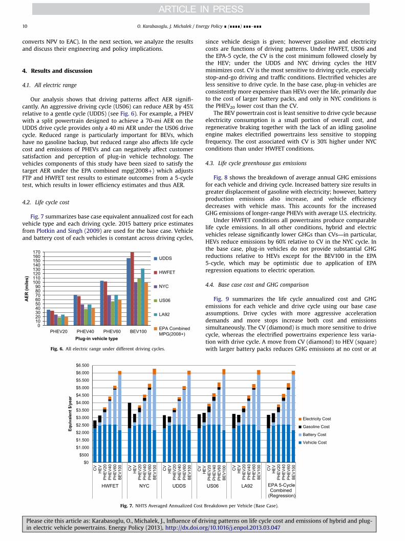
4.1. All electric range

Our analysis shows that driving patterns affect AER signifi-cantly. An aggressive driving cycle (US06) can reduce AER by 45%relative to a gentle cycle (UDDS) (see Fig. 6). For example, a PHEVwith a split powertrain designed to achieve a 70-mi AER on theUDDS drive cycle provides only a 40 mi AER under the US06 drivecycle. Reduced range is particularly important for BEVs, whichhave no gasoline backup, but reduced range also affects life cyclecost and emissions of PHEVs and can negatively affect customersatisfaction and perception of plug-in vehicle technology. Thevehicles components of this study have been sized to satisfy thetarget AER under the EPA combined mpg(2008+) which adjustsFTP and HWFET test results to estimate outcomes from a 5-cycletest, which results in lower efficiency estimates and thus AER.

4.2. Life cycle cost

Fig. 7 summarizes base case equivalent annualized cost for eachvehicle type and each driving cycle. 2015 battery price estimatesfrom Plotkin and Singh (2009) are used for the base case. Vehicleand battery cost of each vehicles is constant across driving cycles,

0102030405060708090

100110120130140150160170

PHEV20 PHEV40 PHEV60 BEV100

AER

(mile

s)

Plug-in vehicle type

UDDS

HWFET

NYC

US06

LA92

EPA Combined MPG(2008+)

Fig. 6. All electric range under different driving cycles.

$0

$500

$1.000

$1.500

$2.000

$2.500

$3.000

$3.500

$4.000

$4.500

$5.000

$5.500

$6.000

$6.500

CV

HE

VP

HE

V20

PH

EV

40P

HE

V60

BE

V10

0

CV

HE

VP

HE

V20

PH

EV

40P

HE

V60

BE

V10

0

CV

HE

VP

HE

V20

PH

EV

40P

HE

V60

BE

V10

0

CV

HWFET NYC UDDS

Equi

vale

nt $

/yea

r

Fig. 7. NHTS Averaged Annualized Cost


since vehicle design is given; however gasoline and electricitycosts are functions of driving patterns. Under HWFET, US06 andthe EPA-5 cycle, the CV is the cost minimum followed closely bythe HEV; under the UDDS and NYC driving cycles the HEVminimizes cost. CV is the most sensitive to driving cycle, especiallystop-and-go driving and traffic conditions. Electrified vehicles areless sensitive to drive cycle. In the base case, plug-in vehicles areconsistently more expensive than HEVs over the life, primarily dueto the cost of larger battery packs, and only in NYC conditions isthe PHEV20 lower cost than the CV.

The BEV powertrain cost is least sensitive to drive cycle becauseelectricity consumption is a small portion of overall cost, andregenerative braking together with the lack of an idling gasolineengine makes electrified powertrains less sensitive to stoppingfrequency. The cost associated with CV is 30% higher under NYCconditions than under HWFET conditions.

4.3. Life cycle greenhouse gas emissions

Fig. 8 shows the breakdown of average annual GHG emissionsfor each vehicle and driving cycle. Increased battery size results ingreater displacement of gasoline with electricity; however, batteryproduction emissions also increase, and vehicle efficiencydecreases with vehicle mass. This accounts for the increasedGHG emissions of longer-range PHEVs with average U.S. electricity.

Under HWFET conditions all powertrains produce comparablelife cycle emissions. In all other conditions, hybrid and electricvehicles release significantly lower GHGs than CVs—in particular,HEVs reduce emissions by 60% relative to CV in the NYC cycle. Inthe base case, plug-in vehicles do not provide substantial GHGreductions relative to HEVs except for the BEV100 in the EPA5-cycle, which may be optimistic due to application of EPAregression equations to electric operation.

4.4. Base case cost and GHG comparison

Fig. 9 summarizes the life cycle annualized cost and GHGemissions for each vehicle and drive cycle using our base caseassumptions. Drive cycles with more aggressive accelerationdemands and more stops increase both cost and emissionssimultaneously. The CV (diamond) is much more sensitive to drivecycle, whereas the electrified powertrains experience less varia-tion with drive cycle. A move from CV (diamond) to HEV (square)with larger battery packs reduces GHG emissions at no cost or at

HE

VP

HE

V20

PH

EV

40P

HE

V60

BE

V10

0

CV

HE

VP

HE

V20

PH

EV

40P

HE

V60

BE

V10

0

CV

HE

VP

HE

V20

PH

EV

40P

HE

V60

BE

V10

0

US06 LA92 EPA 5-Cycle Combined

(Regression)

Electricity Cost

Gasoline Cost

Battery Cost

Vehicle Cost

Breakdown per Vehicle (Base Case).





0.0

1.0

2.0

3.0

4.0

5.0

6.0

CV

HE

VP

HE

V20

PH

EV

40P

HE

V60

BE

V10

0

CV

HE

VP

HE

V20

PH

EV

40P

HE

V60

BE

V10

0

CV

HE

VP

HE

V20

PH

EV

40P

HE

V60

BE

V10

0

CV

HE

VP

HE

V20

PH

EV

40P

HE

V60

BE

V10

0

CV

HE

VP

HE

V20

PH

EV

40P

HE

V60

BE

V10

0

CV

HE

VP

HE

V20

PH

EV

40P

HE

V60

BE

V10

0

HWFET NYC UDDS US06 LA92 EPA 5-Cycle Combined

(Regression)

mt C

O2

eq/y

ear

Electricity Use Gasoline Use Battery ProductionVehicle Production

Fig. 8. NHTS-Averaged Annual GHG Emissions per Vehicle (Base Case).

0

1

2

3

4

5

6

7

$0 $2,000 $4,000 $6,000 $8,000

Ann

ualiz

ed G

HG

s (k

gCO

2eq/

yr)

Annualized Cost ($/yr)

CVHEVPHEV20PHEV40PHEV60BEV100

HWFET

UDDSUS06

LA92

NYC

Fig. 9. Annualized cost vs. annual GHG emissions for various vehicles and drive cycles.Shapes indicate vehicle powertrain. Colors indicate drive cycle.

0.2

0.3

0.4

0 50 100

Ave

rage

kgC

O2e

q/m

i

Daily Distance (miles)

HWFET

BEV100

0.2

0.3

0.4

0 50 100

Ave

rage

kgC

O2e

q/m

i


NYC

PHEV20PHEV40PHEV60

CV

HEV PHEV20

PHEV40HEV

BEV100

Fig. 10. Life cycle GHG per mile under HWFET and NYC driving patterns for avariety of daily driving distances (to show detail, y-axis does not cross at zero). TheCV has 0.75 kgCO2 eq/mi on the NYC cycle.

$0.2

$0.3

$0.4

$0.5

$0.6

0 50 100

Ann

ualiz

ed $

/mi


NYC

$0.2

$0.3

$0.4

$0.5

$0.6

0 50 100

Ann

ualiz

ed $

/mi


HWFET

Fig. 11. The net annualized cost per mile under HWFET and NYC driving patternsfor a variety of daily driving distances (to show detail, y-axis does not cross at zero).


modest cost, depending on the drive cycle. A move from HEV tothe plug-in powertrains with larger battery packs reduces orincreases GHGs, depending on the vehicle and drive cycle, butcomes at a substantial increase in costs.

4.5. Cost and GHGs per mile for different daily driving distances andpatterns

Fig. 10 shows average life cycle GHG emissions per lifetime mileand annualized cost per annual mile traveled as a function of dailydistance traveled for the two contrasting driving conditions:HWFET and NYC, assuming one charge per day and the samedriving distance every day. GHG emissions per mile vary withdaily distance traveled for PHEVs because distance driven betweencharges affects the portion of travel that can be propelled usingelectricity in place of gasoline. If a PHEV is driven further than itsAER, it will begin to consume gasoline. The resulting trends aresimilar to the trends identified by Shiau et al. (2009): PHEVs withsmall battery packs have lower emissions when charged

Please cite this article as: Karabasoglu, O., Michalek, J., Influence of driving patterns on life cycle cost and emissions of hybrid and plug-in electric vehicle powertrains. Energy Policy (2013), http://dx.doi.org/10.1016/j.enpol.2013.03.047i





frequently and driven primarily in CD mode but may have higheremissions if charged infrequently.

The cost curves in Fig. 11 show a decline of annualized cost/mile with daily driving distance, which results from capital cost ofinitial vehicle and battery purchase comprising a larger portion oftotal cost for short daily driving distances, which imply longvehicle life and discounted future fuel costs. The curves have lessoverlap in this case, and dominant vehicles align with NHTS-averaged estimates in Fig. 7. Under HWFET conditions the rankingof cost competitive vehicles (CV, HEV, PHEV20, PHEV40, PHEV60,BEV100) follows increasing battery capacity. Under NYC condi-tions, HEV and PHEV20 are lower cost than CV. In both cases, BEVsincrease the costs significantly.

5. Sensitivity analysis

Fig. 12 summarizes sensitivity of annualized cost to gasoline price,electricity price, vehicle and battery price, carbon tax price (GHGvalue), and discount rate. We focus on comparing two contrastingcases: HWFET which consists of high speed and low acceleration, andNYC which consists of low speed and stop-and-go city driving. Fig. 10ashows the HWFET and NYC EAC breakdown from the base case(Fig. 7). All other cases show the base case as faded bars and displayhow the results would change under alternative assumptions using

$0

$1,000

$2,000

$3,000

$4,000

$5,000

$6,000

$7,000

CV

HEV

PH

EV20

PH

EV40

PH

EV60

HWFET

$0

$1,000

$2,000

$3,000

$4,000

$5,000

$6,000

$7,000

CV

HEV

PH

EV20

PH

EV40

PH

EV60

BEV1

00 CV

HEV

PH

EV20

PH

EV40

PH

EV60

BEV1

00

HWFET NYC

Vehicle Cost

Battery Cost

Gas Cost

Elec. Cost

$0

$1,000

$2,000

$3,000

$4,000

$5,000

$6,000

$7,000

CV

HEV

PH

EV20

PH

EV40

PH

EV60

HWFE

$0

$1,000

$2,000

$3,000

$4,000

$5,000

$6,000

$7,000

CV

HEV

PH

EV20

PH

EV40

PH

EV60

BEV1

00 CV

HEV

PH

EV20

PH

EV40

PH

EV60

BEV1

00

HWFET NYC

Fig.12. Sensitivity analysis for life cycle equivalent annualized cost under HWFET and NY(e) GHG value and (f) Discount rate.


error bars. Fig. 10b shows that increasing gasoline prices affect CV costmost dramatically and makes plug-in technology more cost competi-tive; however, large battery pack vehicles remain higher cost. Fig. 10cshows that electricity price affects the cost of plug-in vehicles withlarge battery packs most; however, a five-fold increase in electric pricehas a notably smaller overall effect that does not change ranking.Fig. 10d emphasizes that vehicle and battery costs have a criticalimpact on the cost benefits of plug-in vehicles. Near term 2015 vehiclecosts estimated by Plotkin and Singh of Argonne National Laboratory(ANL2015) suggest that plug-in vehicles with large battery packs aremore expensive than HEVs regardless of driving cycle, but Departmentof Energy targets for costs in 2030 (DOE2030), which ANL calls “veryoptimistic” (Plotkin and Singh, 2009), would result in more compar-able costs. Fig. 10e reveals that while high carbon prices would havenon-negligible effects on life cycle costs, they would do little to changethe relative costs of the powertrain options except for the relativelylarge penalty to CVs in NYC conditions. Fig. 10f examines the effect ofvarying consumer discount rate. Higher discount rates are less favor-able to plug-in vehicles, whose savings are delayed to future years, butdo not change rank ordering.

Fig. 13 summarizes the effect of electricity source on life cycleGHG emissions. Electricity source varies substantially with locationand charge timing (Sioshansi and Denholm, 2009), is difficult toknow regionally with certainty (Weber et al., 2010), and is typicallynot under the consumer's control. Electricity from coal-fired power

BEV1

00 CV

HEV

PH

EV20

PH

EV40

PH

EV60

BEV1

00

NYC

BEV1

00 CV

HEV

PH

EV20

PH

EV40

PH

EV60

BEV1

00

T NYC

$0

$1,000

$2,000

$3,000

$4,000

$5,000

$6,000

$7,000

CV

HEV

PH

EV20

PH

EV40

PH

EV60

BEV1

00 CV

HEV

PH

EV20

PH

EV40

PH

EV60

BEV1

00

HWFET NYC

$0

$1,000

$2,000

$3,000

$4,000

$5,000

$6,000

$7,000

CV

HEV

PH

EV20

PH

EV40

PH

EV60

BEV1

00 CV

HEV

PH

EV20

PH

EV40

PH

EV60

BEV1

00

HWFET NYC

C drive cycles. (a) Base case, (b) Gasoline price, (c) Electricity price, (d) Vehicle data,





0

1

2

3

4

5

6

7C

VH

EV

PH

EV

20P

HE

V40

PH

EV

60B

EV

100

CV

HE

VP

HE

V20

PH

EV

40P

HE

V60

BE

V10

0

HWFET NYC

Vehicle ProductionBattery ProductionGasoline UseElectricity Use

0

1

2

3

4

5

6

7

CV

HE

VP

HE

V20

PH

EV

40P

HE

V60

BE

V10

0

CV

HE

VP

HE

V20

PH

EV

40P

HE

V60

BE

V10

0

HWFET NYC

mt C

O2

eq/y

ear

Fig. 13. Sensitivity analysis for life cycle GHG emissions. (a) Base case and (b) Grid mix.


plants lead to increased emissions from plug-in vehicles, whereaslow-carbon electricity sources such as nuclear, wind, hydro, and solarpower, result in substantial reductions in life cycle GHG emissionsfrom plug-in vehicles relative to today's U.S. average grid mix. Themarginal electricity used to charge plug-in vehicles will typically notbe nuclear, which is usually run as base load generation, and use ofrenewable energy is subject to constraints from the intermittent andvariable nature of renewable energy sources, so the zero-emissioncases (labeled “Nuclear”) serve as lower bounds.

6. Conclusions

Customer vehicle purchasing decisions are in part guided by EPAfuel economy and AER estimates based on standard laboratory testdriving cycles. However, diverse real-world driving conditions candeviate substantially from laboratory conditions, affecting whichvehicle technologies are most cost effective at reducing GHG emis-sions for each driver. As such, the choice of driving cycle for testingnecessarily preferences some vehicle designs over others. This effecthas become more pronounced with the introduction of hybrid andplug-in powertrains because factors like regenerative braking andengine idling affect the relative importance of aggressive and stop-and-go driving conditions on system efficiency. Compared to cycleslike NYC, test drive cycles UDDS and HWFET, used for corporateaverage fuel economy (CAFE) tests, underestimate relative cost andGHG benefits of hybrid and plug-in vehicles.

With the introduction of hybrid and plug-in vehicles, it has becomemore important that the right vehicles are targeted to the right drivers.Drivers who travel in NYC conditions could cut lifetime costs by up to20% and cut GHG emissions 60% by selecting hybrid vehicles instead ofconventional vehicles, while for HWFET drivers conventional vehiclesprovide a lower cost option with a much smaller GHG penalty. CVowners observe more variability in cost and emissions subject todriving conditions, while HEVs offer the most robust, cost effectiveconfiguration across the driving patterns tested.

When comparing HEVs to PHEVs under the average U.S. grid mix,it is clear that most of the GHG-reduction benefit of PHEVs comesfrom hybridization, and relatively little additional benefit can beachieved through plugging in. HEVs provide an optimal or nearoptimal economic and environmental choice for any driving cycle.However, given a substantially decarbonized electricity grid plug-invehicles could reduce life cycle GHG emissions across all drivingcycles, and lower battery costs combined with high gasoline priceswould make plug-in vehicles more economically competitive.


7. Policy implications

These results have several key policy implications. First, thebenefits of plug-in vehicles vary dramatically from driver to driverdepending on drive cycle (driving style, traffic, road networks, etc.).While hybrid and plug-in vehicles offer little GHG benefit at highercost for highway driving (HWFET), they can offer dramatic GHGreductions and cost savings in NYC driving with frequent stops andidling. Electrification will have more positive impact if targeted todrivers who travel primarily in NYC-like conditions rather thanHWFET-like conditions. Government could play a role through infor-mation campaigns, driver education, as well as modification to fueleconomy labels. The new labels already contain a lot of information,but several possibilities could help target the right drivers: First, thelabel could report several additional characteristic driving cyclesbesides the city and highway mileage reported now. The label designwould need to balance the need to avoid overwhelming the consumer,and more research on this would be needed to determine the bestbalance. Second, the smartphone QR code available on the new labelscurrently takes the consumer to a general website that describes thelabel in more detail. This website could instead offer interactiveinformation for a wider range of driving conditions and evenpotentially use in-vehicle or smartphone GPS to measure the con-sumer's driving style, VMT, and local gasoline prices, using thisinformation to give customized estimates for individual drivers.Privacy concerns would need to be addressed in such a system.Adoption by urban drivers may be limited by lower access todedicated off-street parking and a higher proportion of renters wholack authority to install charging infrastructure (Traut et al., 2013;Axsen and Kurani, 2012a,b).

Second, our results suggest that the choice of standardized testused to assess vehicle efficiency for window labels and for CAFEstandards can have an important effect on the measured benefit ofhybrid and plug-in vehicles relative to conventional vehicles.While choice of testing protocol has always had impact on therelative benefits of vehicles, the unique features of hybrid andelectric vehicle powertrains and their importance in certain typesof driving amplify this impact and the potential for bias that couldsystemically underestimate the benefits of hybridization andelectrification, influencing adoption rates and corporate strategyfor compliance with CAFE standards. Furthermore, vehicles opti-mized to score well on EPA tests may score less well in real-worlddriving. Our results suggest that with the presence of hybrid andelectric vehicles in the marketplace, the test cycles used to assessfuel efficiency – while substantially improved from the old teststhat are still used for CAFE standards – should be reexamined tominimize bias. This could be accomplished, for example, using anational collection of representative GPS data to assess a distribu-tion of driving conditions, followed by simulation, testing, andoptimization to identify a set of tests that produces fuel efficiencyestimates across powertrain types that most closely matchesestimates using a representative distribution of on-road GPS data.In particular, CAFE standards are still based on old UDDS andHWFET tests that produce estimates with about 20% lower fuelconsumption for CV, 30% lower for HEV, and 40% lower for plug-invehicles than the EPA 5-cycle regression tests. The CAFE measure-ment is about 60% lower fuel consuming for CVs and 30% lower forhybrid and electric vehicles than the NYC test. The CAFE testsartificially inflate fuel economy estimates and do so unevenly fordifferent vehicle technologies. Using a common test for CAFEstandards and window labels – one that is as representative aspossible of the resulting efficiency experienced by US driversacross vehicle technologies – would help reduce bias againstcertain technologies as well as confusion about why the high fuelefficiency standards cited by politicians fail to match the reality ofthe vehicle fleet observed by consumers.






Third, as suggested in prior studies (Shiau et al., 2010, 2009;Michalek et al., 2011; Traut et al., 2012; Peterson and Michalek, 2013),HEVs and small-battery PHEVs provide comparable GHG reductions atlower cost than large-battery PHEVs or BEVs with today's electricitygrid. This holds true across the driving cycles we tested. In particular,in NYC conditions HEVs show the lowest cost and GHG emissions. Thisis because hybridization (regenerative braking, efficient engine opera-tion, Atkinson cycle, engine off at idle, etc.) offers most of the GHGbenefit, and additional benefits of using electricity rather than gasolineas the energy source are dependent on grid decarbonization. Currentfederal and state policy favors large battery packs, but this ismisaligned with potential for GHG reductions (Michalek et al., 2011).In fact, given binding CAFE standards plug-in vehicle subsidies mayproduce no net benefit unless they succeed in stimulating a break-through that leads to cost competitive plug-in vehicles and sustainablemainstream adoption that would not have happened otherwise(Peterson and Michalek, 2013; Congressional Budget Office, 2012).

Table A1Vehicle component specifications.

Mass breakdown Units HEV PHEV

Vehicle glider/body mass kg 815 815Powertrain mass kg 609 754Vehicle curb mass kg 1424 1569Driver mass kg 80 80Total mass kg 1504 1649

EngineMax. power kW 73 73Engine scale 1 1Block mass kg 108 108Radiator mass kg 6 6Tank mass kg 20 20Fuel mass kg 43 43Total mass of engine block kg 177 177

MotorMax. power kW 60 78Motor scale 1.0 1.3Motor mass kg 35 46Controller mass kg 5 7Total mass of motor block kg 40 52

Motor 2Max. power kW 30 30Motor mass kg 20 20Controller mass kg 5 5Total mass of motor 2 kg 25 25

BatteryTechnology NiMH Li-ioParallel cell array 1 5Number of cells in series 168 92Total # cells 168 460Cell capacity Ah 7 6Nominal output voltage V 1.2 3.6Output voltage V 202 331Energy capacity kW h 1.3 9.9Packaging factor 1.3 1.3SOC min % 30 30SOC max % 90 90SOC init % 60 90/3SOC target % 60 30Battery swing % 0.6Mass of each cell kg 0.4 0.4Total mass of battery block kg 84 217

Other ComponentsElectrical accessories kg 18 18Exhaust mass kg 30 30Planetary gear mass/gear mass kg 40 40Mechanical accessories kg 35 35Wheel mass kg 140 140Final drive mass kg 20 20Torque coupling kgAlternator and controller kg


Finally, government fleet purchases should account for the antici-pated driving conditions of vehicles when selecting powertrain type.

8. Limitations and future work

There are many factors that may affect the lifetime cost and lifecycle emissions of vehicles. In this work we have addressed drivecycle and distance. Climate may also have a substantial effect onvehicle efficiency, range, and battery life due to climate control,battery thermal management, and sensitivity of battery degrada-tion to temperature (Barnitt et al., 2010). Terrain may also affectelectrified powertrain designs differently, although all drivingcycles presented here are on flat ground.

Vehicle design choices could also influence results. We focus onEREV PHEVs because the broad space of control parameters fordefining a blended operation PHEV makes results too dependenton assumptions (each control strategy will perform better on some

20 PHEV40 PHEV60 BEV100 CV

815 815 815 815978 1212 1450 5561793 2027 2265 137180 80 80 801873 2107 2345 1451

73 73 1101 1 1.5108 108 1666 6 620 20 2043 43 43177 177 234

88 98 1201.5 1.6 2.051 57 707 8 1059 65 80

30 3020 205 525 25

n Li-ion Li-ion Li-ion10 14 2592 100 100920 1400 25006 6 63.6 3.6 3.6331 360 36019.9 30.2 54.01.3 1.3 1.330 30 3090 90 90

0 90/30 90/30 90/3030 30 300.6 0.6 0.60.4 0.4 0.4435 662 1182 22

18 18 18 1830 30 3040 40 7535 35 0140 140 140 14020 20 20 20

10 107





120

140

160Engine Hot Efficiency Map (Torque) - Points

3.73754e-006

2.49

4.98

7.48

9.97

121517202225273032

35 37


drive cycles than others). But blended operation PHEVs could bemore competitive in some cases, especially for low-range PHEVs. Thebattery degradation model used in this study is based on laboratory-tested A123 LiFePO4 cells at room temperature. The data ignoretemperature variation and calendar fade, they do not account for thehigher c-rate implied by more aggressive driving cycles, and they donot examine other chemistries, which can have degradation char-acteristics more sensitive to state of charge and other factors.Degradation also affects vehicle performance (Markel and Simpson,2006), which can prevent the vehicle from satisfying some drivecycles and acceleration tests later in the vehicle's life.

We assume a single charge per day for the PHEV simulations, andwe ignore range limitations of the BEV100, which in practice can besubstantial (Neubauer et al., 2012). Multiple daily charges wouldincrease the benefits of PHEVs and extend the applicability of BEVs.Further, we ignore differences in maintenance, insurance and charginginfrastructure costs across vehicle types and focus only on the splithybrid drivetrain—results for series and parallel designs and forblended control strategies may vary somewhat. We also ignore anysalvage value of the battery pack at end of life as well as opportunitiesfor energy arbitrage in vehicle to grid applications, which are expectedto be small (Peterson et al., 2010). We account only for GHG emissionsand ignore other life cycle emissions and impacts, and we assume thatCO2 tax costs are passed through the supply chain to the vehiclecustomer. We ignore government subsidies, which reduce costsobserved by consumers but transfer these costs to taxpayers ratherthan eliminating them. With government subsidies, plug-in vehiclesare somewhat more attractive purchase options for consumers. Finally,

Table A2Performance of vehicles.

Acceleration time (s)

CV 10.2HEV 10.3PHEV20 CD mode 10.2

CS mode 9.3PHEV40 CD mode 10.1

CS mode 8.1PHEV60 CD mode 10.1

CS mode 8.3BEV100 CD mode 10.1

0 100 200 300 400 500 600-50

0

50

100

150

200

Speed (rad/s)

Torq

ue (N

m)

Engine Hot Efficiency Map (Torque) - Points

3.42034e-006

3.42034e-006

3.42034e-006 3.42034e-006

2.28

2.28 2.28

2.28 2.28 2.28

4.56

4.56 4.56

4.56 4.56 4.56

6.84

6.84 6.84

6.84 6.84 6.84

9.12

9.12 9.12

9.12 9.12 9.12

11

11 11

11 11 11

14

14 14

14 14 14

16

16 16

16 16 16

18

18 18

18 18 18

21

21 21

2121

21

23

23 23

2323

23

25

25 25

2525

25

2727

27

27

27

27 27

30 30

3030

30

30 32

32

32 32

32

34

Max TrqMin TrqMax Eff (Torque based)Max Eff (Power based)Eff. Map

Fig. A1. Engine efficiency map of CV (%) (Argonne National Laboratory, 2008).


advancements in technology and other changes, such as gasolineprices, grid mix, vehicle efficiency, driving patterns, and public policywill affect cost and environmental comparisons in the future.

Acknowledgements

Wewould like to thank to Elizabeth Traut for processing the NHTSdata, Norman Shiau and Nikhil Kaushal for their input on vehiclesimulation, and the members of Design Decisions Laboratory andVehicle Electrification Group at Carnegie Mellon for fruitful discus-sions and useful feedback. This work was supported in part byNational Science Foundation CAREER grant #0747911, Ford MotorCompany, and Toyota Motor Corporation. The opinions expressed arethose of the authors and not necessarily those of the sponsors.

Appendix

Tables A1 and A2Figs. A1–A5

0 50 100 150 200 250 300 350 400 450 500-20

0

20

40

60

80

100

Speed (rad/s)

Torq

ue (N

m)

3.73754e-006 3.73754e-0062.49 2.49 2.494.98 4.98 4.987.48 7.48 7.489.97 9.97 9.9712 12 1215 15 1517 17 1720 20 2022 22 2225 25 2527 27 2730 30

3032 32

32

3535

35

Max TrqMin TrqMax Eff (Torque based)Max Eff (Power based)Eff. Map

Fig. A2. Engine efficiency map of HEV (%) (Argonne National Laboratory, 2008).

-800 -600 -400 -200 0 200 400 600 800-600

-400

-200

0

200

400

600

Speed (rad/s)

Torq

ue (N

m)

Motor Efficiency Map (Torque)

3737

73

37

73

3740

4040

40

04

4044

4444

44

4444

4848

4848

84

48

25

5252

52

25

5256

5656

56

65

56

60

0660

06

6006

64

4664

64

6446

68

6868

68

6886

71

7117

71

7171

75

7575

75

7575

79

79

97

79

79

79

8383

38

38

8383

83 8383

38

87

87

8787

87

87

87

87

87

78

87

87

87

8787

87

87

87

87

87

91

91

9191

91

91

91

91

Propeling Max Torque CurveRegen Max Torque CurveEff. Map

Fig. A3. Motor efficiency map of HEV and PHEVs (%) (Argonne National Laboratory,2008).





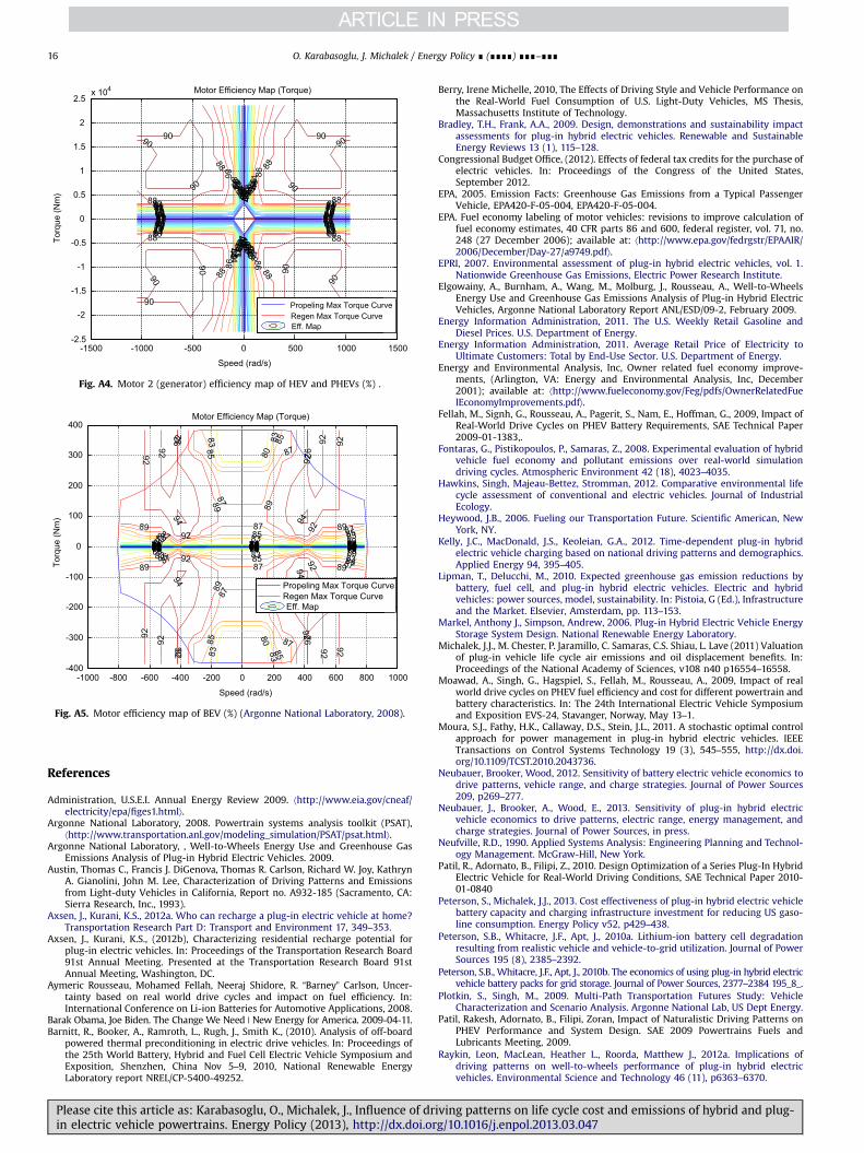
-1500 -1000 -500 0 500 1000 1500-2.5

-2

-1.5

-1

-0.5

0

0.5

1

1.5

2

2.5x 104

Speed (rad/s)

Torq

ue (N

m)


57

57

57

57

57

57

57

57

59

59

59

59

59

59

59

59

61

61

61

61

61

61

61

61

64

64

64

64

64

64

64

64

66

66

6666

66

66

66

66

68

68

6868

68

68

68

68

70

70

7070

70

70

70

7073

73

73

73

73

73

73

7375

75

75

75

75

75

75

75

77

77

7777

77

77

77

77

79

79

7979

79

79

79

79

81

81

8181

81

81

81

81

84

84

84

84

84

84

84

84

86

86

8686

86

86

86

86

88

88

88

88

88

88

88

88

90

90

90

90

90

90

90

90

90

90

90

90Propeling Max Torque CurveRegen Max Torque CurveEff. Map

Fig. A4. Motor 2 (generator) efficiency map of HEV and PHEVs (%) .

-1000 -800 -600 -400 -200 0 200 400 600 800 1000-400

-300

-200

-100

0

100

200

300

400

Speed (rad/s)

Torq

ue (N

m)


60 60 6060 60 6062 62 6262 62 6265 65 6565 65 6567 67 6767 67 6769 69 6969 69 6971 71 7171 71 7174 74 7474 74 7476 76 7676 76 7678 78 7878 78 78

80

80

80 80 8080 80 80

83 83

83 83

83 83 83

83 83 83

85

85

85

85

85 85 85

85 85 85

87

87

87

87

8787 87

8787 87

89

89

89

89

89

89

89

89

92

92

92

92

92

92

92

92

92 92

9292

92

9292

92

92

92

92 92

9494

94

94

Propeling Max Torque CurveRegen Max Torque CurveEff. Map

Fig. A5. Motor efficiency map of BEV (%) (Argonne National Laboratory, 2008).


References

Administration, U.S.E.I. Annual Energy Review 2009. ⟨http://www.eia.gov/cneaf/electricity/epa/figes1.html⟩.

Argonne National Laboratory, 2008. Powertrain systems analysis toolkit (PSAT),⟨http://www.transportation.anl.gov/modeling_simulation/PSAT/psat.html⟩.

Argonne National Laboratory, , Well-to-Wheels Energy Use and Greenhouse GasEmissions Analysis of Plug-in Hybrid Electric Vehicles. 2009.

Austin, Thomas C., Francis J. DiGenova, Thomas R. Carlson, Richard W. Joy, KathrynA. Gianolini, John M. Lee, Characterization of Driving Patterns and Emissionsfrom Light-duty Vehicles in California, Report no. A932-185 (Sacramento, CA:Sierra Research, Inc., 1993).

Axsen, J., Kurani, K.S., 2012a. Who can recharge a plug-in electric vehicle at home?Transportation Research Part D: Transport and Environment 17, 349–353.

Axsen, J., Kurani, K.S., (2012b), Characterizing residential recharge potential forplug-in electric vehicles. In: Proceedings of the Transportation Research Board91st Annual Meeting. Presented at the Transportation Research Board 91stAnnual Meeting, Washington, DC.

Aymeric Rousseau, Mohamed Fellah, Neeraj Shidore, R. “Barney” Carlson, Uncer-tainty based on real world drive cycles and impact on fuel efficiency. In:International Conference on Li-ion Batteries for Automotive Applications, 2008.

Barak Obama, Joe Biden. The Change We Need | New Energy for America. 2009-04-11.Barnitt, R., Booker, A., Ramroth, L., Rugh, J., Smith K., (2010). Analysis of off-board

powered thermal preconditioning in electric drive vehicles. In: Proceedings ofthe 25th World Battery, Hybrid and Fuel Cell Electric Vehicle Symposium andExposition, Shenzhen, China Nov 5–9, 2010, National Renewable EnergyLaboratory report NREL/CP-5400-49252.


Berry, Irene Michelle, 2010, The Effects of Driving Style and Vehicle Performance onthe Real-World Fuel Consumption of U.S. Light-Duty Vehicles, MS Thesis,Massachusetts Institute of Technology.

Bradley, T.H., Frank, A.A., 2009. Design, demonstrations and sustainability impactassessments for plug-in hybrid electric vehicles. Renewable and SustainableEnergy Reviews 13 (1), 115–128.

Congressional Budget Office, (2012). Effects of federal tax credits for the purchase ofelectric vehicles. In: Proceedings of the Congress of the United States,September 2012.

EPA, 2005. Emission Facts: Greenhouse Gas Emissions from a Typical PassengerVehicle, EPA420-F-05-004, EPA420-F-05-004.

EPA. Fuel economy labeling of motor vehicles: revisions to improve calculation offuel economy estimates, 40 CFR parts 86 and 600, federal register, vol. 71, no.248 (27 December 2006); available at: ⟨http://www.epa.gov/fedrgstr/EPAAIR/2006/December/Day-27/a9749.pdf⟩.

EPRI, 2007. Environmental assessment of plug-in hybrid electric vehicles, vol. 1.Nationwide Greenhouse Gas Emissions, Electric Power Research Institute.

Elgowainy, A., Burnham, A., Wang, M., Molburg, J., Rousseau, A., Well-to-WheelsEnergy Use and Greenhouse Gas Emissions Analysis of Plug-in Hybrid ElectricVehicles, Argonne National Laboratory Report ANL/ESD/09-2, February 2009.

Energy Information Administration, 2011. The U.S. Weekly Retail Gasoline andDiesel Prices. U.S. Department of Energy.

Energy Information Administration, 2011. Average Retail Price of Electricity toUltimate Customers: Total by End-Use Sector. U.S. Department of Energy.

Energy and Environmental Analysis, Inc, Owner related fuel economy improve-ments, (Arlington, VA: Energy and Environmental Analysis, Inc, December2001); available at: ⟨http://www.fueleconomy.gov/Feg/pdfs/OwnerRelatedFuelEconomyImprovements.pdf⟩.

Fellah, M., Signh, G., Rousseau, A., Pagerit, S., Nam, E., Hoffman, G., 2009, Impact ofReal-World Drive Cycles on PHEV Battery Requirements, SAE Technical Paper2009-01-1383,.

Fontaras, G., Pistikopoulos, P., Samaras, Z., 2008. Experimental evaluation of hybridvehicle fuel economy and pollutant emissions over real-world simulationdriving cycles. Atmospheric Environment 42 (18), 4023–4035.

Hawkins, Singh, Majeau-Bettez, Stromman, 2012. Comparative environmental lifecycle assessment of conventional and electric vehicles. Journal of IndustrialEcology.

Heywood, J.B., 2006. Fueling our Transportation Future. Scientific American, NewYork, NY.

Kelly, J.C., MacDonald, J.S., Keoleian, G.A., 2012. Time-dependent plug-in hybridelectric vehicle charging based on national driving patterns and demographics.Applied Energy 94, 395–405.

Lipman, T., Delucchi, M., 2010. Expected greenhouse gas emission reductions bybattery, fuel cell, and plug-in hybrid electric vehicles. Electric and hybridvehicles: power sources, model, sustainability. In: Pistoia, G (Ed.), Infrastructureand the Market. Elsevier, Amsterdam, pp. 113–153.

Markel, Anthony J., Simpson, Andrew, 2006. Plug-in Hybrid Electric Vehicle EnergyStorage System Design. National Renewable Energy Laboratory.

Michalek, J.J., M. Chester, P. Jaramillo, C. Samaras, C.S. Shiau, L. Lave (2011) Valuationof plug-in vehicle life cycle air emissions and oil displacement benefits. In:Proceedings of the National Academy of Sciences, v108 n40 p16554–16558.

Moawad, A., Singh, G., Hagspiel, S., Fellah, M., Rousseau, A., 2009, Impact of realworld drive cycles on PHEV fuel efficiency and cost for different powertrain andbattery characteristics. In: The 24th International Electric Vehicle Symposiumand Exposition EVS-24, Stavanger, Norway, May 13–1.

Moura, S.J., Fathy, H.K., Callaway, D.S., Stein, J.L., 2011. A stochastic optimal controlapproach for power management in plug-in hybrid electric vehicles. IEEETransactions on Control Systems Technology 19 (3), 545–555, http://dx.doi.org/10.1109/TCST.2010.2043736.

Neubauer, Brooker, Wood, 2012. Sensitivity of battery electric vehicle economics todrive patterns, vehicle range, and charge strategies. Journal of Power Sources209, p269–277.

Neubauer, J., Brooker, A., Wood, E., 2013. Sensitivity of plug-in hybrid electricvehicle economics to drive patterns, electric range, energy management, andcharge strategies. Journal of Power Sources, in press.

Neufville, R.D., 1990. Applied Systems Analysis: Engineering Planning and Technol-ogy Management. McGraw-Hill, New York.

Patil, R., Adornato, B., Filipi, Z., 2010. Design Optimization of a Series Plug-In HybridElectric Vehicle for Real-World Driving Conditions, SAE Technical Paper 2010-01-0840

Peterson, S., Michalek, J.J., 2013. Cost effectiveness of plug-in hybrid electric vehiclebattery capacity and charging infrastructure investment for reducing US gaso-line consumption. Energy Policy v52, p429–438.

Peterson, S.B., Whitacre, J.F., Apt, J., 2010a. Lithium-ion battery cell degradationresulting from realistic vehicle and vehicle-to-grid utilization. Journal of PowerSources 195 (8), 2385–2392.

Peterson, S.B., Whitacre, J.F., Apt, J., 2010b. The economics of using plug-in hybrid electricvehicle battery packs for grid storage. Journal of Power Sources, 2377–2384 195_8_.

Plotkin, S., Singh, M., 2009. Multi-Path Transportation Futures Study: VehicleCharacterization and Scenario Analysis. Argonne National Lab, US Dept Energy.

Patil, Rakesh, Adornato, B., Filipi, Zoran, Impact of Naturalistic Driving Patterns onPHEV Performance and System Design. SAE 2009 Powertrains Fuels andLubricants Meeting, 2009.

Raykin, Leon, MacLean, Heather L., Roorda, Matthew J., 2012a. Implications ofdriving patterns on well-to-wheels performance of plug-in hybrid electricvehicles. Environmental Science and Technology 46 (11), p6363–6370.


)http://www.eia.gov/cneaf/electricity/epa/figes1.html*

)http://www.eia.gov/cneaf/electricity/epa/figes1.html*

)http://www.transportation.anl.gov/modeling_simulation/PSAT/psat.html*

http://refhub.elsevier.com/S0301-4215(13)00225-5/sbref1





)http://www.epa.gov/fedrgstr/EPAAIR/2006/December/Day-27/a9749.pdf*

)http://www.epa.gov/fedrgstr/EPAAIR/2006/December/Day-27/a9749.pdf*







)http://www.fueleconomy.gov/Feg/pdfs/OwnerRelatedFuelEconomyImprovements.pdf*

)http://www.fueleconomy.gov/Feg/pdfs/OwnerRelatedFuelEconomyImprovements.pdf*


















http://dx.doi.org/10.1109/TCST.2010.2043736





























Raykin, Leon, Roorda, Matthew J., MacLean, Heather L., 2012b. Impacts of drivingpatterns on tank-to-wheel energy use of plug-in hybrid electric vehicles.Transportation Research Part D: Transport and Environment 17 (3), p243–250.

Samaras, C., Meisterling, K., 2008. Life cycle assessment of greenhouse gasemissions from plug-in hybrid vehicles: implications for policy. EnvironmentalScience & Technology 42 (9), 3170–3176.

Samaras, C., Meisterling, K.s.w., 2008. Life cycle assessment of greenhouse gasemissions from plug-in hybrid vehicles: implications for policy. EnvironmentalScience & Technology 42 (9), 3170–3176.

Sciarretta, A., Guzzella, L., 2007. Control of hybrid electric vehicles. IEEE ControlSystems 27 (2), 60–70, http://dx.doi.org/10.1109/MCS.2007.338280.

Sciarretta, A., Back, M., Guzzella, L., 2004. Optimal control of parallel hybrid electricvehicles. IEEE Transactions on Control Systems Technology 12 (3), 352–363,http://dx.doi.org/10.1109/TCST.2004.824312.

Sharer, P., Leydier, R., Rousseau, A., Impact of Drive Cycle Aggressiveness and Speedon HEVs Fuel Consumption Sensitivity, SAE Technical Paper 2007-01-0281,2007, http://dx.doi.org/10.4271/2007-01-0281.

Shiau, C.-S., Kaushal, N., Hendrickson, C.T., Peterson, S., Whitacre, J., Michalek, J.J.,2010. Optimal plug-in hybrid electric vehicle design and allocation for mini-mum life cycle cost, petroleum consumption, and greenhouse gas emissions.ASME Journal of Mechanical Design, Special Issue on Sustainability, v132 n9p091013 1-11.

Shiau, C.S.N., Samaras, C., Hauffe, R., Michalek, J.J., 2009. Impact of battery weightand charging patterns on the economic and environmental benefits of plug-inhybrid vehicles. Energy Policy 377, 2653–2663.

Shiau, Ching-Shin Norman, Kaushal, Nikhil, Hendrickson, Chris T., Peterson, Scott B.,Whitacre, Jay F., Michalek, Jeremy J., 2010. Optimal plug-in hybrid electricvehicle design and allocation for minimum life cycle cost, petroleum con-sumption, and greenhouse gas emissions. Journal of Mechanical Design 132091013—1 — 11.


Sioshansi, R., Denholm, P., 2009. Emissions impacts and benefits of plug-in hybridelectric vehicles and vehicle-to-grid services. Environmental Science andTechnology 43, 1199–1204.

Southern California Association of Governments; Year 2000 Post-Census RegionalTravel Survey, Fall 2003.

Tate, E.D., The Electrification of the Automobile. 2008.Traut, E., Hendrickson, C., Klampfl, E., Liu, Y., Michalek, J.J., 2012. Optimal design and

allocation of electrified vehicles and dedicated charging infrastructure forminimum life cycle greenhouse gas emissions and cost. Energy Policy 51,524–534.

Traut. E., Cherng. T.W., Hendrickson. C., Michalek. J. (2013) U.S. Residential ChargingPotential for Plug-in Vehicles, Working Paper, Department of MechanicalEngineering, Carnegie Mellon University.

Tulpule, P., Marano, V., Rizzoni, G., Effects of different PHEV control strategies onvehicle performance, American Control Conference, 2009. ACC ‘09., vol., no., pp.3950–3955, 10–12 June 2009 doi: 10.1109/ACC.2009.5160595\.

U.S. Department of Transportation, F.H.A., 2009 National Household Travel Survey.2009.

US Environmental Protection Agency, 2011, ⟨http://www.fueleconomy.gov/feg/label/⟩.

Wang, M., Wu, Y., Elgowainy, A., 2007. GREET 1.7 Fuel-Cycle Model for Transporta-tion Fuels and Vehicle Technologies,. Argonne National Laboratory, Argonne, IL.

Weber, C.L., Jaramillo, P., Marriott, J., Samaras, C., 2010. Life cycle assessment andgrid electricity: what do we know and what can we know? EnvironmentalScience & Technology , http://dx.doi.org/10.1021/es9017909.

Whitefoot, J.W., Ahn, K., Papalambros, P.Y. The case for urban vehicles: powertrainoptimization of a power-split hybrid for fuel economy on multiple drive cycles.In: ASME Conference Proceedings, 2010. (44120): p. 197–204.













http://dx.doi.org/10.1109/MCS.2007.338280






dx.doi.org/doi:10.4271/2007-01-0281





















)http://www.fueleconomy.gov/feg/label/*

)http://www.fueleconomy.gov/feg/label/*



http://dx.doi.org/10.1021/es9017909






influence of driving patterns on life cycle cost and ... · of hybrid and plug-in electric vehicle...

Documents