probability proportional to size sampling of douglas-fir

Probability Proportional to Size Samplingof Douglas-Fir from Aerial Photography

by

Roger Allan Rogers

A THESIS

submitted to

Oregon State University

in partial fulfillment ofthe requirements for the

degree of

Master of Science

June 1972

AN ABSTRACT OF THE THESIS OF

Roger Allan Rogers for the Masters of Science(Name of Student) (Degree)

Forest Management presented on(Major) (Date)

Title: PROBABILITY PROPORTIONAL TO SIZE SAMPLING OF

DOUGLAS-FIR FROM AERIAL PHOTOGRAPHY

Abstract approved by:Dr. David P. Paine

This experiment was designed to investigate the use of volume

estimations from aerial photography and probability proportional to

size (PPS) sample seLection in the development of a practical sam-

pling design for timber volume estimation on small land areas of

Pacific Northwest Douglas -fir (Pseudotsuga menziesii, Franco).

The major problem of measuring exact stand height to predict stand

volume from aerial photos was overcome by the development of two

new volume equations which use percent crown closure, visible

crown diameter and height classes as the independent variables. By

the use of height classes, the photo interpreter is required to sep-

arate stand heights as to tall, medium or short. Equations are

presented for both board- and cubic-foot volumes.

1 L

I

Two computer programs were developed which reduce office

calculations to a minimum. The programs compute photo volumes

per plot, total gross and net volume estimations per area, standard

errors and select the field plots to be sampled.

The sampling design was tested on four test areas, using both

quarter- and one-acre photo plots, and quarter-acre fixed-area and

variable-area field plots at four photo scales. Based on these results

a sample of about 20 field measured quarter-acre field plots com-

bined with a 100 percent photo cruise on 1:7,000 aerial photos would

be expected to produce gross volume estimations for a forty-acre

tract of + 10 percent. at a 68 percent confidence level.

S

S

Probability Proportional to Size Samplingof Douglas-Fir from Aerial Photography

by

Roger Allan Rogers

A THESIS

submitted to

Oregon State University

in partial fulfillment ofthe requirements for the

degree of

Master of Science

June 197Z

APPROVED:

Date thesis is presented

Associate Professor of Forest Managementin charge of major

Head of Department of Forest Management

Dean of Graduate School

Typed by Mona F. Luebbert for Roger Allan Rogers

1

TABLE OF CONTENTS

1. Introduction

2 Literature Review 3

PPS Sampling 3Aerial Photo Volume Tables 5Stand Height 7Scale 8

The Experiment 10Location 10Photography 10Calculation of the Photo Volume Equations 11Computer Programs 15Program AERPPS 15Program FIELD 17Conducting the Experiment 19

Results and Conclusions 28Quarter-Acre Photo Cruise of Test Area 2 28One-Acre Photo Cruise of all Test Areas at

Project Scale 1:7, 000 30Total Volume Estimations for Test Area 2

Using Quarter-Acre Photo and Field Plots 32Total Volume Estimations for Each Test Area

Using One-Acre Photo and Variable AreaField Plots 35

Summary 38Bibliography 40Appendix I 42Appendix II 44

2

LIST OF TABLES

Table Page

Height Classes 15

Quarter-acre photo cruise of test area 29

One-acre photo cruise of all test areas atproject scale 1:7, 000 31

Total volume estimations for test area 2using quarter-acre photo and field plots 33

Total volume estimations for each test areausing one-acre photo and variable areafield plots 36

LIST OF FIGURES

Figure Page

An example of AERPPS output. 18

FIELD output for an individual fixed-areaquarter-acre plot. 20

FIELD output for an individual variablearea plot. 22

FIELD summary table. 23

Test site 2 and quarter-acre grid. 24

Variable plot design. 27

IACKNOWLEDGEMENTS

The author would like to express his appreciation to the follow-

ing people without whose assistance this experiment could not have

been completed:

Dr. David P. Paine and Dr. John F. Bell of the School of

Forestry for their guidance, assistance and critical review.

Robert B. Pope of the Pacific Northwest Forest and Range

Experimental Station for the field data used in developing volume

equations.

Dr. Lyle Calvin and Dr. Norbert A. Hartman of the Statistics

Department for their assistance in the statistical analysis and cri-

tical review respectively.

Mr. Linn H. Scheurman of the Statistics Department for the

design of the random number generator.

Mr. Floyd Forristall for his assistance and guidance in ob-

taining the field measurements.

My wife, Friah, for her patience, support and encouragement

throughout the entire experiment.

I

S

PROBABILITY PROPORTIONAL TOSIZE SAMPLING OF DOUGLAS-FIRFROM AERLAL PHOTOGRAPHY

I. INTRODUCTION

Historically the practice of estimai;ing timber volumes has been

dependent upon some form of sampling design because of the large

populations involved. With the passing of the timber cruiser who

could walk through a forest and estimate the total volume by "eyeba1i,

many sampling methods have been used for volume estimation. The

earliest sampling procedure was strip cruising, where strips of a

given width were inventoried at specified intervals throughout the

forest tract. Later individual plots of many different shapes and sizes

located in some random or systematic manner were used and statisti-

cal analysis made. Most timber estimation is presently done with the

use of either fixed area or variable area plots with or without stratifi-

cation. However, in the case of small tracts of land, 100 percent in-

ventory is still conducted in many cases.

Since the advent of aerial photography, many foresters have be-

lieved that aerial photos should be used for some purpose other than

locating plots in the field. Although many attempts have been made to

incorporate the information presented by the aerial photo into some

practical sampling method for the estimation of timber volumes,

stratification of the forest types and double sampling have developed as

the only advantageous applications of the available information.

In the use of aerial photo plots, foresters can carry stratification

to its limits - each plot is considered as a separate stratum. Much of

the difficulty in incorporating the information available on the aerial

photo into a sampling procedure has been due to some inherent diffi-

culties in measuring three dimensional variables on a two dimensional

s ii r fa c e.

The objective of this experiment was to design and evaluate a

practical sampling procedure incorporating the concept of probability

proportional to size (PPS) sample selection and the variables easily

measured or estimated from modern aerial photos which would be

applicable to the estimation of total volumes of Douglas-fir (Pseudo-

tsuga menziesiiFranco) timber in the Pacific Northwest. Major em-

phasis was placed on application of the inventory to small land tracts.

S

S

II. LITERATURE REVIEW

PPS Sampling

Sampling designs employing probability of sample selection pro-

portional to size (PPS) are not new. The original concept of PPS sam-

pling was presented by Hansen and Hurwitz (1943).

Selection with pps means that, on the average, a primarysampling unit (psu), which is, for example, 5 times aslarge as another will be in the sample 5 times as frequentlyas the other psu. It might appear, at first, that this wouldintroduce a bias in the sample result with some psu's over-represented and others under-represented - and it would,in fact, if no special attention were given to the varyingprobabilities in the estimating or subsampling procedures(Hansen, Hurwitz, and Madow, 1953a, p342).

One of the advantages gained by the use of PPS sampling is that:

for many common populations, and with a fixed number ofprimary units in the sample, a smaller variance will beobtained by sampling with probability proportionate to sizethan by sampling with equal probability. (Hansen, et al.l953b)

Basically, the PPS sampling method consists of three major

steps:

List a quick, subjective estimate of the volume of each sample

unit in the population.

Select, based on probability proportional to size, from the list,

the sample units to be accurately measured.

Make precise measurement of the selected sample units to allow

accurate determination of the value being estimated.

S

S

4

In PPS sampling, 'selection with replacement is necessary in

order to keep the probabilities of selection proportional to the sizes.

(Cochran, 1963, p. 251).

Investigation has demonstrated that better results can be obtained

in PPS sampling with refinement of the subjective estimate of the pri-

mary sample units, Schreuder, Sedransk, and Ware (1968) stated:

It seems possible that inexpensive objective measurementof some concomitant variables might sometimes lead tomore reliable and efficient estimates via a functional re-lationship (between the variable of interest and a concomi-tant variable) than subjective ocular estimation.

In its original form, a major problem arose when PPS sampling

was applied for forest inventory. Schreuder, et al. (1968) explains:

Most of the ordinary procedures for sampling with pro-bability proportional to size require, prior to sampling,a list of sizes of all units in the population. However,for forest inventory, the cost of relocating and re-observing usually makes it inefficient to visit a treemore than once - i. e. to visit once to make a list andidentify trees, then to return to sample.

One method of avoiding the problem of relocating and revisiting the

primary sample unit is outlined in Grosenbaugh1s (1964) Three-P

sampling procedure. Another possible solution was assumed to lie in

the use of aerial photo interpretation of the primary sample units and

application of aerial photo volume tables to obtain an estimate of the

unit's volume.

S

Aerial Photo Volume Tables

Aerial photo volume tables are historically divided into two

classes; stand volume tables and tree volume tables. Stand volume

tables have made use of percent crown closure and height of the stand

as independent variables to predict stand volumes. The advantages of

stand volume tables are that volumes are given directly on a per acre

basis and they are less time-consuming to use, however no information

is given for individual trees and the measurement of stand height is

difficult to obtain.

Tree volume tables use the independent variables of visible

crown diameter and total tree height to predict individual tree volume.

Although information is available on each tree, and their use if more

easily applied to mixed-species and aid aged forests, tree volume

tables are very time-consun- ng to use and measurement of individual

tree height is both difficult and costly.

Aerial photo volume tables were first used in the late 1920!s and

early 193Os. Spurr (1954) sketches the early development of these

tables.

The first aerial photo-volume tables were stand volumetables. They were developed by students of ProfessorHugershoff in Germany between 1925 and 1933 and werebased on only one variable, either total stand height orstand density. In 1929, H. E. Seely, a Canadian, usedtree heights estimated from shadows on aerial photosand 'crude aerial photo stand-volume tables" to approx-imate timber volumes in forest survey work.

6

Pope (1950) was the first to develop stand aerial photo volume

tables for Douglas-fir in the Pacific Northwest. He used the indepen-

dent variables, average stand, total tree height, visible crown dia-

meter and percent crown closure, to predict stand volumes in board

and cubic feet. On four out of seven tests, his photo estimates were

within three percent of the ground estimates and for the remaining

three tests, his results were within ten percent. For the purposes of

these tests, he used the same site-index and density classes for the

construction of his aerial photo volume tables. However, further test-

ing showed that on poorer sites, the photo estimates were 25 to 45 per-

cent lower than the ground estimates, and with poorly-stocked stands,

the photo estimates were 10 to 20 percent higher than the ground esti-

mates.

Pope (1961) later published a new Bet of photo volume tables for

Douglas-fir. With the availability of computers and Grosenbaugh's

(1958) computer program, he was able to expand the possible combin-

ations of variables although he was still limited to nine variables. His

two best equations were:

V = 0. 9233HC + 0. 0070H2C 0. 0086HC2 - 179. 0

and

Vb 0. 9533C2 + 3. 2313HC + 0. 716H2C - 0. 00883HC2+ -3285. 0

where

V Volume per acre in cubic feet

S 7

Vb Volume per acre in board feet

C Percent crown closure of major canopy

H Average height of dominant and codominant trees

His results reflected a standard deviation about the regression line

of+ 3,777 cubic feet per acre and + 26, 312 board feet per acre or

+ 29. 2 and + 34. 8 percent respectively.

Stand Height

The major restriction in the use of aerial photo volume tables

is the requirement for measurement of the stand or tree height. In

measuring height from aerial photos, 'the measurement of parallax

differences is the most widely used method and, once mastered, yields

the most accurate results. " (Spurr, 1954) However, mastering the

measurement of parallax differences is both difficult and time-

consuming. Getchell and Young (1953) conducted experiments which

have shown "it takes between 12 and 18 hours to learn to become

reasonably proficient with height finders, " For many people, com-

plete mastery is never obtained. Studies by Moessner (1955), Spurr

(1960), and Mac Lean and Pope (1961) have found that besides the

inherent difficulties in measuring parallax differences, the major

errors in height measurement are the result of individual operator

ability and personal bias.

Another possible source of error in height measurement is the

effect of tilt in the aerial photos. Pope (1957) found that three degrees

of tilt along the line of flight results in an error of nine percent with

a six-inch lens and increases to 35 percent with a 24-inch lens.

A further complication of accurate height measurement is that

in dense stands of the Pacific Northwest, it is often im-possible to measure stand height at the plot because theground cannot be seen. Here the interpreter must exer-cise his ingenuity, estimating the ground reading byinterpolation or measuring nearby stands with a similarappearance (Pope, 1961).

Scale

Another factor which must be considered whenever aerial photos

are used is the photographic scale. There are several areas where

photo scale may be a possible source of error; accuracy of height

measurement, species identification and ground location may all be

affected. Pope (1957) found in tests of photo scales from 1:2, 500 to

1:20, 000 that errors in measuring tree height were more dependent

upon the individual interpreter than photo scale. However, he noted

indications that species identification became more accurate with the

use of larger scales. Young (1953) also demonstrated the difficulties

of species identification with increasing photo scales.

Errors in ground measurement and location can also be the

result of photo scale. Moessner (1963) found that using 1:16, 000

9

scale aerial photos as much as one-third the average error in direc-

tion and two-thirds the average error in distance experienced in

locating points on the ground can be due to the limitations of photo

scales and techniques.

IIII. THE EXPERIMENT

Lo cation

The test sites used in this experiment are located in McDonald

Forest, near Corvallis, Oregon. This area is typical of the inland

Douglas-fir stands found throughout the Pacific Northwest. Douglas-

fir is the predominant species and the stands range from almost pure

stands of Douglas-fir with a highly scattered population of true fir to

Douglas-fir, non-commercial hardwood mixtures. The majority of

the area is second-growth Douglas = fir, however, there are residual

blocks of old-growth present. The majority of the second-growth

stands are typed as small to large saw timber (i. e. D3 and D4), while

the old-growth is considered large old growth (i. e. D5). Stocking

within the forest ranges from poor to well stocked, with the major

portion being in the medium stocked class (i. e. 40 to 70 percent).

This area was selected because of the range of timber conditions pre-

sent which allow evaluation of the experiment for the commonly found

Douglas-fir stands of the Pacific Northwest.

Photography

The aerial photos used in this experiment were obtained from

H. G. Chickering, Jr. . Consulting Photogrammetrist, Inc., of Eugene,

Oregon. Four photo flights were required to provide complete cover-

10

11

age of the area at the project scales of 1:4, 000, 1:7, 000, 1:10, 000,

and 1:12, 000. For the purpose of calculating the project scale, the

mean elevation of the test areas was considered to be 1, 000 feet above

sea level. The photos were taken with an aerial camera using a

12-inch focal length lens and panchromatic film. The photo flights

were made in July, 1970 during the late morning hours to minimize

th loss of detail due to shadow effects.

The photos received were nine by nine inch format, semi-- -

matte finished on double weight paper. It was decided that these

were the most practical compromise between photos for office and

field use. Upon receipt of the photos, each scale coverage was

checked stereoscopically to insure that 100 percent photo coverage

of the area had been obtained. The photos were found to meet all

specifications and were considered to be of excellent quality.

Calculation of the PhotoVolume Equations

The volume formulas developed for the computer programs

written for this experiment were derived through the use of the com-

puter facilities at Oregon State University. The facilities primarily

used were the CDC 3300 computer and the library stepwise multiple

linear regression analysis program, *STEP. This program allows

for the input of up to eighty variables with up to eighty transformationsS

S

12

being performed on the input variables by the computer. The stepwise

procedure is that

at any stage of the stepwise procedure only one variableis either entered or removed from the equation and avariable to be removed takes priority over one to beadded. The contribution a variable makes in reducingthe variance is considered for all variables in theequation. If the contribution of a particular variableis insignificant, this variable is removed; otherwisethe variance reduction for all variables not in the re-gression is considered. The variable which most signi-ficantly reduces the variance is then added to the equa-tion. If there are no more variables to examine orboth of the above significance tests fail, the algorithmis terminated (OSU Statistical Analysis Program Library,1969).

The data used for calculating these volume equations were fur-

nished by Pope. 1 This was the original data used in 1961 to generate

his stand volume tab'es for Douglas-fir in the Pacific Northwest. One

of the advantages gained by the use of these data was the comparison

with the existing volume formulas to determine if improvement had

occurred.

The original design was to produce volume formulas based on

the use of two independent variables; percent crown closure and visible

crown diameter of the average dominant and codominant trees. It was

thought that visible crown diameter could replace the use of stand

height in previous stand volume tables and therefore all the difficulties

1Pope, Robert B. Unpublished data on aerial photo stand volumetables for Douglas-fir in the Pacific Northwest. Pacific NorthwestForest and Range Expt. Station, Portland, Oregon. n. d.

13

inherent in stand height measurement might be avoided. Twenty-two

linear and quadratic functions and combinations of percent crown clo-

sure and visible crown diameter were investigated. The best equa-

tion derived was:

Vb = 133. 609 - 0. 0068(CC.VCD2) + 9. 279x10 7(CC.VCDZ)Z

- 7. Z2lxlO(CCVCD2)3

where:

Vb = Volume per acre in hundreds of board feet

CC = Percent crown closure of conifers

VCD Average visible crown diameter of the dominant and

codominant conifers

The correlation coefficient of this equation was 0. 757 which

did not compare favorably with the 0. 918 reported by Pope (1961) based

on the same data but using average stand height in place of visible

crown diameter. When the formula was applied to variables outside

the upper bounds of the data, unrealistic results were also noted. It

became obvious that stand height was a significant variable and would

have to be included in the equation. With the inclusion of stand height

as an independent variable, the following Iormulas were derived.

Vb = 30. 5566 + 1. 99O3x1O5(HT CC.VCD)

and

IV 39. 363 + 7. 6999x10 4(HT CC) - 1. O766xlO(HTZ.

-5 2 -22CC) + 1. 0540x10 (HT CC.VCD) + 4. 0882xl0

2 3(HT CCVCD)

where

V Volume per acre in tens of cubic feet

HT = Average height of the dominant and codominant conifers,

and the other variables are those listed previously.

The correlation coefficient for this board-foot volume equation

was 0. 932 and for the cubic-foot volume equation, 0. 911. These com-

pare with the coefficients of 0. 918 and 0. 904 reported by Pope (1961).

While the increases in the correlation coefficients demonstrated that

these new volume equations were an improvement over existing for-

mulas, the addition of stand height as a variable had defeated the

original goal and increased the difficulty of obtaining the required

measurements.

One method available to reduce the difficult and time-consuming

requirement for measuring stand height was to substitute an estimate,

based on stereoscopic viewing, of stand height for the actual measure-

ment. This estimation was further simplified through the use of

height classes. Four height classes (including 0 for no trees present)

were finally selected. These are shown in Table 1.. There were two

major justifications for their use. The first was the belief that any

precision loss caused by grouping into height classes would be offset

14

15

TABLE 1. HEIGHT CLASSES

Height Class Range Midpoint

0 No trees on plot1 70 29. 9 feet 100 feet

2 130 - 189. 9 feet 160 feet3 190 250. 0 feet 220 feet

by reduced time and cost factors in comparison to photo measured

stand heights, and that any loss of accuracy would be relatively small.

The second justification was that the volumes produced by these

formulas were designed to replace the subjective estimates in the first

step of PPS sampling and although the desired goal was to produce

more accurate estimates, these volumes are only to be considered as

estimates in themselves.

Computer Programs

Two computer programs were written for this experiment;

AERPPS and FIELD. These programs are written in Fortran IV

machine language for use by the Oregon State University CDC 3300

computer.

Program AERPPS

Program AERPPS is a computer program designed to utilize

the input data from a 100-percent photo cruise of a designated area to

S

S

16

calculate individual plot and total area volumes, select plots for field

measurement by the PPS sampling method, and calculate the mean of

each variable, of the plot volumes, and the population variance and

coefficient of variation. The following limitations are placed upon the

program user:

Plot size must be between 0. 1 and 9 acres,

Total area size must be less than 1000 acres.

The maximum number of photo plots in the total area is 500.

The maximum desired sample size is 500 plots.

The program user must also select the unit of volume (i. e. board or

cubic feet) desired, and must indicate the estimated sample size

desired for further field measurement.

The input variables for each plot are percent crown closure of

the conifers present (expressed as real numbers, i. e. 27. 5% is entered

as 27. 5), visible crown diameter of the average dominant and codomi-

nant conifers (expressed in thousandths of an inch as measured from

the photo) and the height class of the average dominant and codominant

conifers on the plot. The input data are converted to their actual

values by the computer and the plot volumes calculated.

A random number generator is included in the program to create

the necessary random numbers required by the PPS sampling method.

The limitations placed upon the generator are that no number can be

larger than the total estimated volume of the area and any number

I

ii ii.E (x1Y1)ji=1

17

larger than the largest individual plot volume is replaced by a zero

which indicates automatic rejection for field measurement of any plot

with which it is paired. An example of the computer output of program

AERPPS is shown in Figure L

Program FIELD

Program FIELD is a computer program designed to utilize the

field measurement data with the 100-percent photo cruise data to ob-

tain the final estimated gross and net total volumes for each designated

area and calculate the standard error of each volume estimation. The

program user has several options available (i. e. fixed area or variable

area field plots, board-foot or cubic-foct volumes, and two types of

output listings discussed below). The field data inputs required for this

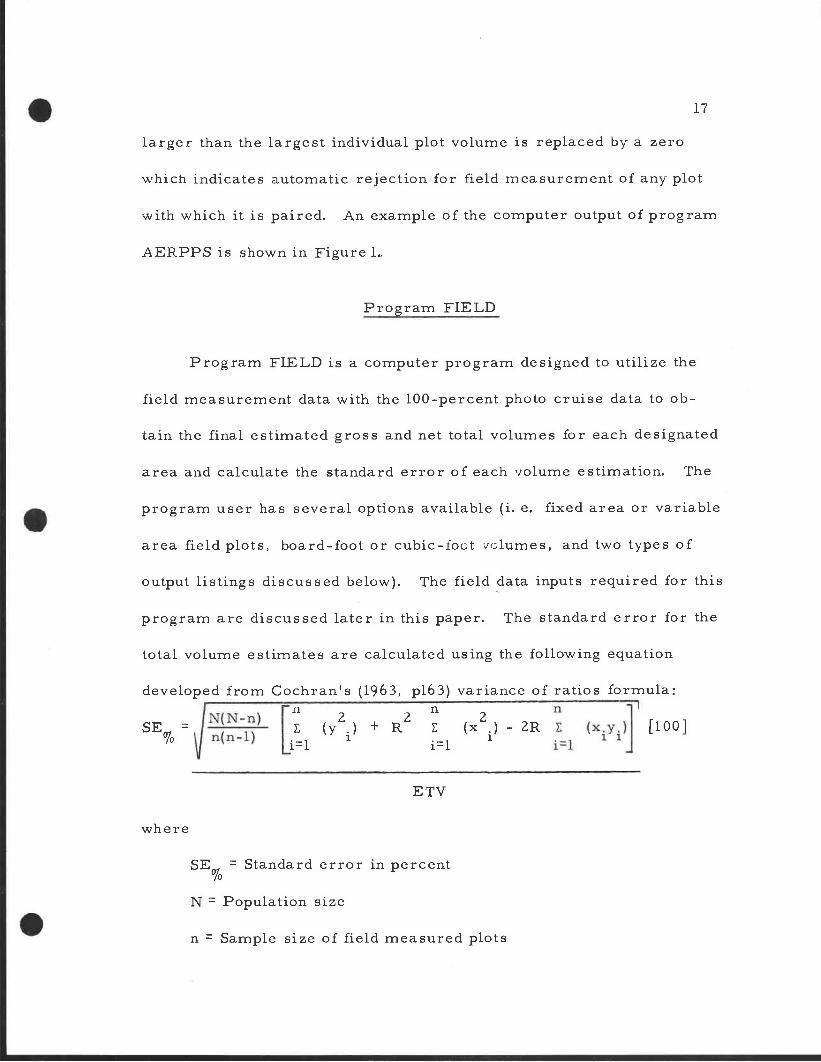
program are discussed later in this paper. The standard error for the

total volume estimates are calculated using the following equation

developed from Cochran's (1963, p16 3) variance of ratios formula:11 fl

SE (y) + RZ (x2.) - ZR [100]% . 1i-i i-1

ETV

where

SE = Standard error in percent

N = Population size

n = Sample size of field measured plots

NR:7-OS25 ACRE

TOTAL EST ii ME: 1529ZY MEAN PLOT VOLUME9MEAN CC34. MEAN V C MEAN MT CLASSZ.POP. VARIAN 9X 100, 000 ICIENT OF VARIATJON:68

Figure 1. e of AERPPS Output

MC DONALD FOREST, CORVALLIS, ORE T11S R 5W SECTION 8 TEST AREA 2SCALE 1: 6694 PHOTO U-843-70 2.46-1-6,1-8TEST AREA SIZE:40. 00 ACRES PLOT SIZE: . S

PLOT NO. %CC VCD HT CLASS EST BD FT VOLUME FIELD CHECKPER PLOT X 100

0101 20 22. 3 2 64.5 NO0 102 10 18. 1 2 30. 7 NO0103 5 16. 7 2 18. 3 NO0104 50 19. 5 2 132. 0 YES0105 55 20. 9 2 154, 2 NO0106 25 18. 1 2 65. 4 NO0107 35 18. 1 2 88. 5 NO1008 10 13. 9 2 25. 4 NO1009 10 13 9 25. 4 NO1010 15 13.9 1 18. 0 NO1011 10 13.9 2 25.4 NO10 12 20 15. 3 2 46. 7 NO1013 4 16, 7 2 16. 2 NO10 14 25 16. 7 2 60. 9 NO10 15 30 16. 7 2 7 1. 6 YES1016 40 15. 3 2 85. 8 NO

D FT VOLU 100 5. 6 BD FT X 1009 D17. 6FT 1

CE: 4345. 4 COEFF .97%

An Exampi

y. = Sampled plot field measured volume

x. = Sampled plot photo estimated volume

yii 1

R = Ratio of the means

19

ETV = Total estimated volume

The program user has the option of selecting one of two output

formats. One format lists the individual plot calculations and then

provides a summary table. The second option produces only the sum-

mary table. Figure 2 is an example of the individual plot data for a

fixed-area plot, Figure 3 is for a variable area plot and Figure 4 is

an example of a summary table.

Conducting the Experiment

Upon obtaining the photos, the general area was reviewed stereo-

scopically to determine the best locations for test sites which would

take advantage of the maximum variation within the forest. Each test

site was to be a square of forty acres. Each corner of the test sites

was located on the 1:12, 000 photos with a photo templet and then trans-

ferred to the larger scale photos by observation. Later measurement

in the field showed that the sites were not exactly forty acres in size,

because of the point differences in photo scale due to ground elevation

differences.

, x.1

i= 1

NET VOLBIDET

1 0

936439460739581284

011001085

049

1370

1632904

0386808981477413

1353842477

12165299BD FT

MC DONALD FOREST, CORVALLIS, ORE T11S ROSW SECTION 8 TEST AREA 2

TOTAL GROSS VOLUME: 16246BD FT TOTAL NET VOLUME: 1Figure 2. FIELD Output for an Individual Fixed-Area Quarter-Acre Plot

SCALE 1:

SP

6694

PLOT NR:07 08DBH HT

PHOTO NR:07-OSU-843-70 246- 1-6, 1-8

GROSS VOL %CULLBDFT

DF 25. 5 138 923 00DF 24.8 140 936 0DF 19,9 114 462 5DF 19. 1 130 460 0DF 22. 7 133 739 0DF 20,9 129 581 0DF 17. 0 105 284 0DF 9.0 37 0 0DF 26.6 138 1100 0DF 27. 3 136 1085 0DF 7.6 35 0 0DF 10. 8 76 50 2DF 13.6 85 137 0DF 8.1 42 0 0DF 31.9 142 1632 0DF 25. 4 135 904 0WF 10.4 44 0 0DF 19. 5 108 386 0DF 24. 1 132 808 0DF 26.2 134 981 0DF 20. 1 118 477 0DF 19.2 116 413 0DF 29. 3 136 1353 0DF 24. 1 138 842 0DF 20.0 118 477 0DF 27.8 142 1216 0

21

Initially, it was decided to investigate the use of fixed-area plots

within each test site. Because of the requirement of a 100-percent

ground cruise of the plots selected for field measurement, one-quarter

acre plots were selected. Each test site was divided into a 160 plot

grid utilizing 16 divisions in the east-west direction and 10 divisions in

the north- south direction. Each grid was drawn directly on the photo

and a standardized numbering system was employed. Figure 5 is one

test site and its associated grid with the grid lines darkened and

widened for emphasis.

Beginning with the smallest scale photos, the author conducted

a 100- percent photo cruise of each site at each photo scale, recording

the following variables for each plot; visible crown diameter of the

average dominant and codominant conifers, percent crown closure for

all conifers present and the estimated height class for the average

dominant and codominant conifers, percent crown closure for

all conifers present and the estimated height class for the average

dominant and codominant conifers. Visible crown diameter was mea-

sured in thousandths of an inch by the use of a crown dot wedge. Per-

cent crown closure was estimated using the standard method of "tree

cramming" to the nearest five percent. Height class was ocularly

estimated using the height class listed in Table 1.

MC DONA T, CORV uS RO5W SECTIONSCALE 1: HOTO NR:7-OStJ-843-PLO T:05- L TREE TOTAL POINTS: 5SP DBH GROSS V NET VOL GROSS

GROSS VOLUME PER ACRE: 71410BD FT NET VOLUME PER ACRE: 71043BD FT

Figure 3. FIELD Output for an Individual Variable Area Plot

LD FORES

669402 TOTA

HT

ALLIS, ORE TP

COUNT: 43OL %CtJLL

BDFT BDFT

8 TEST AREA 270 246-1-6, 1-8BAF:27. 2V-BAR NET V-BAR

DF 22.9 116 649 0 649 373.0 373.0DF 23.7 118 727 0 727 390. 1 390. 1DF 28. 2 129 1113 0 1113 421. 8 421. 8DF 18. 8 96 347 0 347 295. 9 295. 9DF 20. 3 108 439 0 439 321. 0 321. 0DF 31. 1 128 1297 0 1297 404. 1 404. 1DF 20. 6 110 50 1 0 501 355. 8 355. 8DF 32. 1 132 1522 0 1522 445. 1 445. 1DF 32. 5 134 1544 0 1544 440. 5 440. 5DF 21. 1 U5 522 0 522 353. 3 353. 3DF 22. 7 120 670 0 670 391. 8 39 1. 8WF 37. 2 138 2306 5 2191 502. 2 477. 1DF 14. 2 79 129 0 129 192.. 8 192. 8

TOTAL PHOTO VOL: 1924500 ED F!TOTAL GROSS VOL: 1562994 ED FTTOTAL NET VOL: 1360987 ED FTSTANDARD ERROR IN GROSS VOLUMSTANDARD ERROR IN NET VOLUME:

PLOT PHOTOVOL

GROSSVOL

01-07 41340 5402203-03 73400 3088103-07 111540 5787903-08 59010 3735404-03 49240 6763905-0? 58480 71410

*---:--****** SUMMARY TABLE FOR TEST AREA 2 *********

MC DONALD FOREST, CORVALLIS, ORE T11S RO5W SECTION 8SCALE 1: 6694 PHOTO NR:7-OSIJ-843-70 246- 1-6, 1-8TOTAL NUMBER OF PLOTS: 40

NETVOL

GROSSRATIO

NETRATIO

52545 1. 307 1. 27130355 .421 .41425052 . 519 . 22531799 . 633 . 53967 140 1.. 374 1. 36471043 1. 221 1. 215

E: 412942 BD FT 26. 420%5 18469 ED FT 38. 095%

Figure 4. FIELD Summary Table

'I

1.

vi

ri

-t.

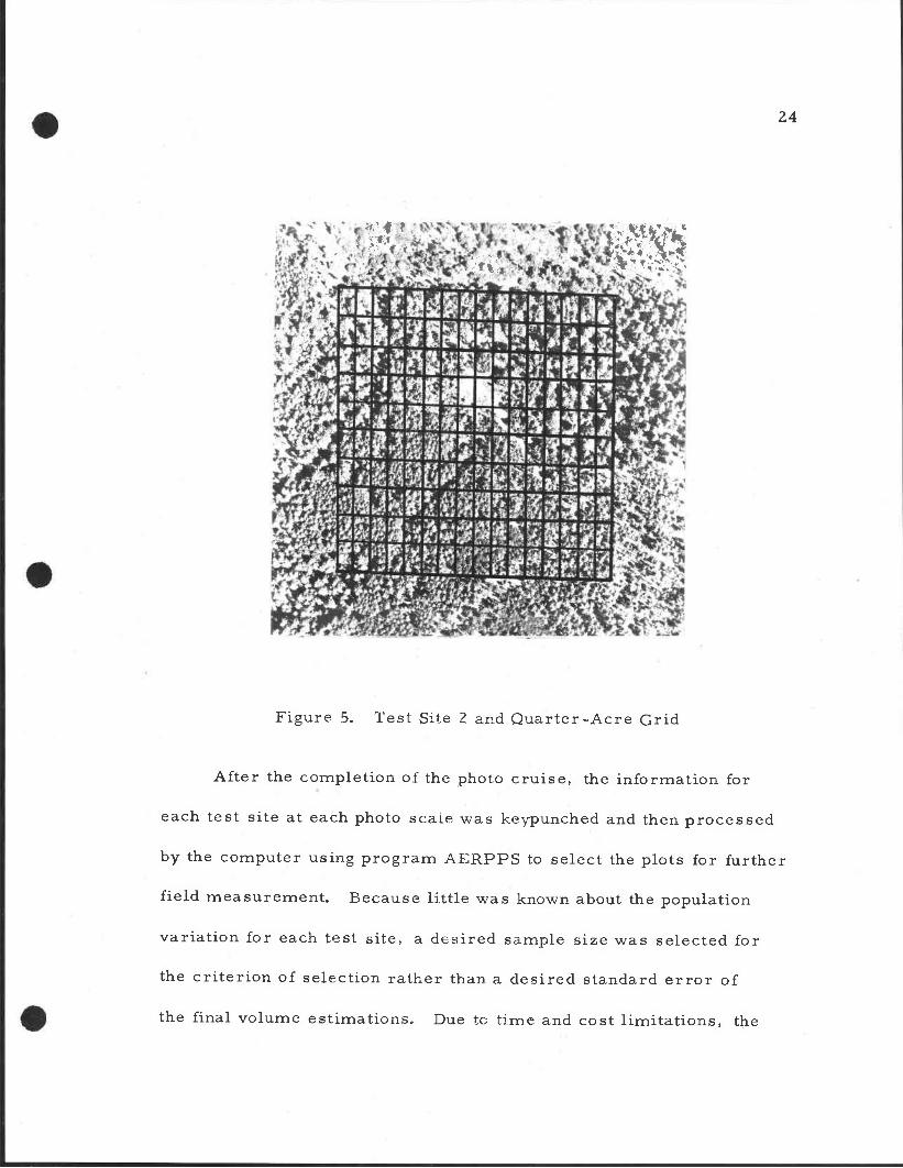
Figure 5. Test Site 2 and QuarterAcre Grid

After the completion of the photo cruise, the information for

each test site at each photo scale was keypunched and then processed

by the computer using program AERPPS to select the plots for further

field measurement. Because little was known about the population

variation for each test site, a desired sample size was selected for

the criterion of selection rather than a desired standard error of

the final volume estimations. Due to time and cost limitations, the

24

desired sample size was set at five plots per test site, per photo

scale.

At this point, the decision was made to expand the experiment

to include field measurements using variable area plots. To facilitate

this expansion, photo plots of one acre were selected. The photo

cruise information already gathered was adjusted to make each block

of four one-quarter plots into a one-acre plot by using the arithmetic

mean of the percent crown closure, and the maximum value of the

visible crown diameter and height class of the one-quarter acre plots.

The desired sample size was again set at five plots per test site and

computer selection of the plots to be field measured was made by the

computer program AERPPS.

Field measurement of the selected plots was conducted in the

following manner:

For test site 2, each set of selected fixed-area plots for each

photo scale were measured.

For all four test sites, each set of one-acre plots selected at

photo scale 1:7, 000 were measured.

To measure the fixed-area plots, each corner of the plot was

located and marked on the ground from interpretation of the photos

in the field. The plot was then systematically measured, recording

for each conifer, the species, diameter at breast height (DBH), total

height and percent cull. DBH was measured by a diameter tape and

total height was measured by a tape and clinometer. Percent cull

25

S

26was estimated from visible indicators and the prior knowledge and

experience of the cruisers.

For the variable plots to be measured in the field, a five point

sampling plot was established (see Figure 6).

In designing the five point layout, was established at 34°l2'

to insure that the four outer points fall within the one-acre photo plot

of this shape. The distance ID is a variable distance dependent upon

the average DBH of the stand. This is because the area of a variable

area plot is dependent upon DBH and thus, it insures that the trees

selected are within the photo plot being sampled. Tree counts were

made on every point and measurements were taken on the center point.

Tree selection for both tree count and measurement was made with a

wide.-angle Spiegel- Relaskop calibrated for a basal area factor of 27.2.

At each point, the trees were identified by species. At the center

point, the same measurements were made on the count trees as were

made on the fixed-area plots. Location of the center point in the field

was determined from interpretation of the photos in the field. Upon

completion of the field measurements, board-foot volumes were

assigned to each measured tree using the volume tables developed by

Bruce and Girard (n. d.). Cubic-foot volumes were assigned from

Table 2 in Agriculture Handbook No. 92 (1955). All the information

gathered on each field plot was then keypunched and program FIELD

was used to obtain the estimated total gross and net volumes for each

test site and photo scale combination measured.

NORTH

POINT 2 POINT 3

where

POINT 4 POINT 5VALUES FOR D

Average flRT-T nf t2nd ft

Figure 6. Variable Plot Design

27

12 inches 28 inches 100

32 inches 94

36 inches 87

40 inches 80

44 inches 7348 inches 66

tZ2 nrHrc (r (vtr-, An

IV. RESULTS AND CONCLUSIONS

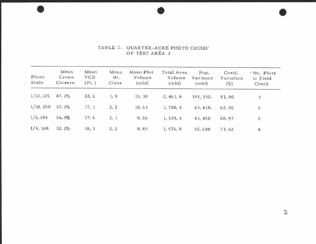
Quarter-Acre Photo Cruise of Test Area 2

The results of the photo cruise of test area 2 using fixed area

plots of one-quarter acre are presented in Table 2. This area was

measured at each photo scale, beginning with the smallest scale.

There are two major points of interest in these results. First, there

does not seem to be a noticeable effect of photo scale when the co-

efficients of variation are considered for the three larger photo scales.

However, there appears to be a noticeable increase in variation be-

tween the results of the 1:12, 125 scale photos and the other, larger

scales. There are two suspected sources of this difference. On

small scale aerial photos, it becomes increasingly difficult to distin-

guish between conifers and hardwoods on panchromatic film and cor-

rectly identify each species. This difficulty is reflected in the in-

creased mean percent crown closure at the smallest photo scale. The

second possible source is the difficulty in separating the intermixed

crowns of adjacent conifers. This is suggested by the relatively large

mean visible crown diameter noted at this photo scale.

When the 1:4, 348 scale results are analyzed, there are two

noticeable effects from interpretation of the larger scale photos.

There is a tendency to underestimate the percent crown closure and

overestimate the visible crown diameter, both of which are reflected

28

Cfl

LflIn

r

TABLE 2. QU ACRE PHOTO CRUISEOF REAZ

Mean Mean Mean Mean Plot Total Area Pop. Coeff. No. PlotsPhoto Crown VCD Ht. Volume Volume Variance Variation to FieldScale Closure (Ft. ) Class (mbf) (mbf) (mbf) (%) Check

i/iz, 125 47. 2% 22, 6 1. 9 15. 39 2, 46 L 8 155, 330. 8 1. 00

i/io, 250 37. 2% 17. 1 2. 2 10. 63 1,700. 4 43, 410. 62. 00

1/6,694 34. 9% 17, 6 2. 1 9. 56 1, 529. 4 43, 450 68. 97

1/4, 348 32. 2% 18, 3 2. 2 9. 85 1, 576. 8 52, 640 73. 62

30

in the means shown. These tendencies can be directly related to

overcompensation by the interpreter of the extreme parallax exper-

ienced in photos of this scale.

The second point of interest in these results is the actual num-

ber of plots to be field measured that were selected by the computer.

Although five plots had been requested for each photo scale, at only

two photo scales, were five plots selected. This is a result of using

the selection rule presented in Grosenbaugh's (1964) Three-P sampling

procedure and is dependent upon the random numbers generated by

the random number generator. Over a large number of selections

from the same population, Bell (1970) has shown that the average

selected number and the desired number will be nearly equal, although

in each individual selection the number may vary considerably. This

effect is most noticeable when the desired sample size is very small,

and each plot represents a large proportion of the total sample. One

methQd available to avoid this problem is the use of the selection

procedures outlined by Hartley (1966).

One-Acre Photo Cruise of AllTest Areas at Project

Scale 1:7, 000

The results of the photo cruise of all four test areas using

fixed area plots of one acre at a photo project scale of 1:7, 000 are

presented in Table 3.. The same effects of photo scale are noted

-N

)en

TABLE 3. ONE-ACRE PHOTO CRUISE OF ALL TEST AREASAT PROJECT SCALE 1:7, 000

MeanTest CrownArea Closure

MeanVCD(Ft. )

ManHt.

Class

Mean PlotVolume(mbf)

Total AreaVolume(mbf)

Pop.Variance

(mbf)

Coeff. No. PlotsVariation to Field

(%) Check

26. 0% 26. 5 2. 8 62. 08 2, 483. 1 614, 600. 39. 94

34. 9% 19. 7 2. 4 48. 11 1,924. 5 463, 740. 44. 76

32. 8% 18. 4 2. 0 34. 75 1, 390. 0 167, 540. 37. 25

22. 5% 15. 6 2. 2 25. 85 1, 034. 1 225, 588. 58. 13

I

I

32

in these results, and although valid, these are also the result of the

method used in gathering the data. These data were obtained by com-

bination of blocks of four one-quarter acre plots as explained earlier.

If comparison of the results for test area 2 at each plot size is

made, the following effects of plot size are noted. There is a slight

increase in the mean height class when one-acre plots are used,

however both methods would consider the mean height class to be

class 2. The increase in mean visible crown diameter for the one-

acre plots is due to the use of the average dominant and codominant

cLinifers for this measurement and the smaller opportunity for a

ItclumptT effect to occur on a one-acre plot. As would be expected,

there is a decrease in the population coefficient of variation when

one-acre plots are compared to the quarter acre plots, which can be

also explained by the lack of clumping.

In these results, there is also a noticeable difference between

the desired and actual number of plots selected for field measurement.

However in this case, three of the four computer runs produced

sample sizes in excess of the desired number.

Total Volume Estimations forTest Area 2 Using Quarter-Acre

Photo and Field Plots

The total gross and net volume estimations for test area 2 and

their related standard errors are presented in Table 4. These

. . .FOR TESFIELD p

TABLE 4.. TOTAL VOLUME ESTIMATIONS T AREA 2USING QUARTER-ACRE PHOTO AND LOTS

No. Plots Gross Standard Net StandardPhoto Field Total Photo Total Gross Total Net Error ErrorScale Checked Vol (mbf) Vol (mbf) Vol (mbf) mbf % mbf

i/iz, 125 2, 461. 8 1, 206. 5 705. 8 587. 7 48. 7 668. 9 94. 8

i/b, 250 1, 700. 4 1, 559. 6 1,468.9 333.6 21.4 324.0 22. 1

1/6, 694 1, 529. 2 1, 658. 7 1 , 60 1. 8 304. 9 18. 4 305. 3 19. 1

1/4, 348 1, 576. 8 1, 098. 2 1,024. 9 375. 7 34. 2 348. 1 34. 0

S

S

34

estimations are based on the use of one-quarter acre photo and field

plots at each of the photo scale.

The large standard error of both gross (48. 7%) and net (94. 8%)

total volume estimations at photo scale 1:12, 125 can be explained as a

combination of the inherent interpretation difficulties previously ex-

plained and the small number of field measured plots. The same con-

clusions can be made when considering the standard errors of 34. 2%

and 34. 0% for the gross and net total volume estimations made from

the 1:4, 348 scale photos. Consideration of these two standard errors

for net volume emphasizes one limitation of the use of aerial photos

for timber volume estimation and the small size of the sample

measured in the field. There is no recognized manner in which to

estimate net plot volume from the photos and therefore the selection

must be based upon the estimated gross volumes. When this is com-

bined with a small sample size, there is a greater probability of error

in net volume due to the random possibility of having large amounts of

cull present on the few plots selected. Increasing the sample size

will remove this possibility in most cases.

When the results at 1:10, 250 and 1:6. 694 scale photos are com-

pared, the differences in the standard error for both the gross and

net estimated total volumes are not significant. Although this one

test would suggest that the best photo scale would be the 1:6, 694 scale,

there are several related factors which must now be considered. Con.

35

sideration must now be given to characteristics which are not directly

related to the sampling design. These characteristics include the num-r

ber of test sites which can be covered by one set of stereo photos and

the resultant cost, and the ease of interpretation, and time reductions

in interpretation in both the office and the field which may arise from

use of the larger scale and their resultant cost benefits. These char-

acteristics, while important for consideration, are beyond the scope

of this experiment.

Total Volume Estimations forEach Test Area ijsing One-Acre

Photo and Variable Area Field Plots

The total gross and net volume estimations for each test area

and their related standard errors are presented in Table 5. These

estimations are based on the use of one-acre photo plots at a project

scale of 1:7, 000 and variable area field plots.

Although the use of variable area plots is the only economic

method of sampling one-acre plots in the field, there is a likelihood

of increasing the standard error of the total volume estimation be-

cause there is not a 100-percent enumeration of the plot population as

is the case when one-quarter acre plots are used. This can be seen

in the increase in the standard error of the total volume for test area

2 using variable area field plots as compared to one-quarter acre

plots (i. e. 26. 4% versus 18. 4% for total gross volume).

. . .IMATIONSVARIABL

TABLE 5. TOTAL VOLUME EST FOR EACH TEST AREAUSING ONE-ACRE PHOTO AND E AREA FIELD PLOTS

No. PlotsTest FieldArea Checked

4

Total PhotoVol (mbf)

2, 483. 1

1, 924. 5

1., 390. 0

1, 034. 1

Total GrossVol (mbf)

3, 498. 9

1, 563. 0

1, 338. 7

900. 0

Total NetVol (mbf)

1, 701. 9

1, 361. 0

1, 28 1. 8

764. 3

Gross StandardError

rnbf %

333.4 9. 5

412. 9 26. 4

199. 7 14. 9

403. 2 44. 8

Net StandardError

mbf

192. 7 11. 3

5 18. 5 38. 1

199, 0 15. 1

319. 6 41. 8

37

Another limitation in the use of variable area field plots arises

when consideration is given to the number of plots required to reduce

the standard error to a given percentage. If the practical estimate of

quadrupling the plot number to halve the standard error is applied and

the desired percentage of standard error is ten percent or less, then

it would take twenty one-quarter acre plots versus more than twenty-

four one-acre plots to achieve this goal. In the case of a forty acre

test site, this would require more than fifty percent of the ground area

to be field measured. It is doubtful that any type of justification could

be made for this intense a sampling scheme in the case of volume es-

timation.

V. SUMMARY

This experiment was designed to create and evaluate a procedure

for combining the use of aerial photo interpretation and the probability

proportional to size sampling method into a simple and efficient means

of estimating total gross and net timber volumes on small tracts of

land in the Pacific Northwest Douglas-fir region. One basic design

criterion was to use wherever possible modern computers to reduce

the amount of calculation time required. Through the se of aerial

photo interpretation, it was thought that the problem of visiting each

plot twice as would normally be required in a PPS sampling design

would be avoided.

The primary difficulty in past use of aerial photo interpretation

for estimating volumes has been the requirement in the photo volume

tables for measurement of tree height. Originally, it was thought

that this could be avoided by the use of other, more easily measured

variables, however it was found that the substitution of height classes

could be used in place of actual measured heights. Two new volume

equations, one for board-foot and one for cubic-foot volumes, were

developed by the use of stepwise multiple regression analysis. These

formulas require the interpreter to estimate percent crown closure,

and height class of the average dominant and codorninant conifers and

measure the average visible crown diameter of the average dominant

38

39

and codominant conifers on every photo plot. These are simple para-

meters for any photo interpreter to obtain from modern aerial photos.

The procedures and two computer programs developed in this

experiment are applicable throughout the Pacific Northwest Douglas-

fir region and provide the user with several alternatives. The user

can choose either board- or cubic-foot volumes, plot sizes ranging

from one-tenth to nine acres and either fixed area or variable area

field plots. Although the two computer programs were designed for

a CDC 3300 computer, they are written in Fortran IV language and

make use of common library subfunctions available on most modern

computers.

Evaluation of the procedure was conducted using four, forty acre

test sites simulating four timber sales. The results of this evaluation

indicate that the use of one-quarter acre photo and field plots and

photo scales between 1:7, 000 and 1:10, 000 provide the best volume

estimations among the scales and plot types examined. On the basis

of the field evaluations, approximately ZO one-quarter acre field plots

would be expected to produce gross timber volume estimations with

ten percent error at a 68 percent confidence level. -This corn-.

pares favorably with the present use of 40 to 80 field plots, dependent

upon the population coefficient of variation.

S

40

8p.

BIBLIOGRAPHY

Bell, John F. 1970. Sampling with unequal probabilities to estimatecubic-foot volume growth for immature Douglas-fir on perma-nent sample plots. Doctoral dissertation. Ann Arbor. Univer-sity of Michigan, 1970. 112 numb, leaves.

Bruce, Donald and James Girard. n. d. Board foot volume tablesbased on total height. Portland, Oregon. Mason, Bruce andGirard. 45p.

Cochran, William G. 1963. Sampling Techniques. 2d ed. New York.John Wiley and Sons. 4O3p.

Getchell, Willis A. and Harold E. Young. 1953. Length of time nec-essary to attain proficiency with height finders on air photos.University of Maine Forestry Department Technical NotesNo. 23. 2p.

Grosenbaugh, L. R. 1958. The elusive formula of best fit: A com-prehensive new machine program. Southern Forest Experimen-tal Station. Occasional Paper No. 158. 9p.

1964. STX-Fortran 4 Program--for estimates oftree populations from 3P sample-tree-measurements. U. S.Forest Service Research Paper PSWJ3?

Hansen, Morris H. and William N. Hurwitz. 1943. On the theoryof sampling fr-n finite populations. Ann. Math. Statist.14:330- 362.

Hansen, Morris H., William N. Hurwitz and William G. Madow.1953a. Sample survey Methods and Theory, Volume 1- Methodsand Applications. New York. John Wiley and Sons. 638p.

l953b. Sample Survey Methods and Theory,Volume 2- Theory. New York. John Wiley and Sons. 332p.

Hartley, H. 0. 1966. Systematic sampling with unequal probabilityand without replacement. American Statistical AssociationJournal. 61:739-748.

MacLean, Cohn D. and Robert B. Pope. 1961. Bias in the estima-tion of stand height from aerial photos. Forestry Chronicle37:160-161.

Moessner, Karl E. 1955. The accuracy of stand height measure-ments on aerial photos in the Rocky Mountains. IntermountainForest and Range Expt. Station. Research Note No. 25. Sp.

Pope, Robert B. 1950. Aerial Photo Volume Tables. Photo. Eng.6(3):325-327.

1957. The eflect of photo scale on accuracy offorest measurements. Photo. Eng. 869-873.

1961. Aerial photo volume tables for Douglas-firin the Pacific Northwest. Portland, Oregon. Pacific North-west Forest and Range Expt. Station. Research Paper No. 214.

41

1962. Constructing aerial photo stand volumetables. Portland, Oregon. Pacific Northwest Forest andRange Expt. Station. Research Paper No. 49. 25p.

Sçhreuder, Hans T., Joseph Sedransk and Kenneth D. Ware. 1968.3-P Sampling and some alternatives, L Forest Science14(4);429 -452.

Spurr, Stephen. 1954. History of forest photogrammetry and aerialmapping. Photo. Eng. 20:551-560.

1960. Photogramrnetry and Photo-Interpretation.Zd ed. New York. The Ronald Press. 472p.

U. S. Department of Agriculture. 1955. Volume Tables for PacificNorthwest trees. Washington. D. C. n. p. (AgriculturalHandbook No. 92).

yates, Thomas L. (ed.). 1969. OSU Statistical analysis programlibrary. Corvallis, Oregon. Department of Statistics. Ore-gon State University. Zd rev.

Young, Harold E. 1953. Tree counts on air photos in Maine. Photo.Eng. :111-116.

4

APPENDIX I

Data Deck for AERPPS

First Card - Total number of test areas and choice of volume

units.

Column

1 - 3 Total number of test areas.

5 1 - board foot volumes.

2 - cubic foot volumes.

Second Card - Test area header card.

Column

1 - 32 Location of test area.

33 - 35 Township.

37 - 39 Range.

41 42 Section.

44 - 45 Test area identification number.

47 - 5 1 Photo scale reciprocal.

53 - 80 Photo identification.

Third Card - Test area dimension card.

Column

Plot size in acres with implied decimal.

(i. e. 1/4 acre plot is 0025)

6 - 10 Test area size in acres with implied decimal.

42

lZ - 15

17 - 19

Fourth Card -

Colurri n

(i. e. 100. 50 acres is 10050)

Total number of plots in test area.

Desired size for field measured sample.

Plot data card.

1 4 Plot identification.

6 7 Percent crown closure to the nearest five

percent.

9 - 11 Average visible crown diameter measured

from the photo in thousandths of an inch.

(i. e. 0. 0405 inches is 405)

13 Height Class

Each new plot requires a new fourth card.

Each new test area begins with a new second card.

43

7

9

S

S

APPENDIX I I

Data Deck for FIELD

First Card Total number of test areas and option selection.

Column

1 - Number of test areas.

5 1 fixed area plots.

2 variable area plots.

1 board foot volumes.

2 cubic foot volumes.

1 individual plot information and summary.

2 summary only.

Test area header card.

Location of test area.

Town3hip.

Range.

Section.

Test area identification number.

Photo scale reciprocal.

Photo identification.

Third Card (fixed area plots only) - Test area dimension card.

44

Second Card

Column

1 32

33 35

37 - 39

41 - 42

44 - 45

47 - 51

53 - 80

2

3

Column

1 - Number of field measured plots.

4 - 10 Total estimated photo volume for test area.

12 16 Plot size in acres with implied decimal.

(i. e. 1/4 acre plot is 0025)

18 - 20 Total number of plots. (i. e. 50 plots is 050)

Fourth Card (fixed area plots only) - Individual plot data card.

Column

1 - 5 Plot identification.

6 - 10 Photo estimated plot volume. (nearest whole

unit of volume)

Fifth Card (fixed area plots only) - Individual tree data card.

Column

1 - 2 Species Identification.

4 - 6 DBH with implied decimal. (i. e. 10. 5 inches

is 105)

8 - 10 Total tree height to nearest foot.

12 - 14 Percent cull estimated.

16 - 19 Gross volume (nearest whole unit of volume).

Third Card (variable area plots) - Test area dimension card.

Co lum n

1 - Basal area factor with implied decimal.

(i. e. 27. 5 BAF is 275)

45

a

9

5

46

Total number of points counted in the test area.

Total number of points measured in the test

area.

Number of field measured plots.

Total estimated photo volume for test area.

Total number of plots in test area.

Fourth Card (variable area plots) - Individual plot data card.

Column

1 - Plot identification.

7 - 11 Photo estimated plot volume. (nearest whole

unit of volume)

13 - 14 Form class with implied decimal (i. e. 0. 78

is 78)

16 - 17 Total number of points per plot.

19 - 20 Tree count on point 1.








5-

8-

11 - 12

14 - 20

22 - 24



Fifth Card (variable area plots) - Individual tree data card.

Co lurn n

1 - Z Species identification.

4 - 6 DBH with implied decimal. (i. e. 10. 5 inches

is 105)

10 Total tree height to nearest foot.

12 - 14 Percent cull estimated.

16 - 19 Gross volume (nearest whole unit of volume).

The last card for every plot must be an end of file card.

Each new plot begins with a new fourth card.

Each new test area begins with a new second card.

47

probability proportional to size sampling of douglas-fir

Documents