1 Authors are Power Professor of Agribusiness, Associate Professor and Research Associate,respectively, in the Morrison School of Agribusiness, Arizona State University, Mesa, AZ. 85212. Contact author: trichards@asu.edu. Support for this project from the Food Systems Research Groupat the University of Wisconsin, Madison is gratefully acknowledged.

Price Promotion by Multi-Product Retailers

Timothy J. Richards, Paul M. Patterson, and Luis Padilla1

Paper presented at the

First Biennial Conference of the Food Systems Research Group

Madison, Wisconsin, June 26 - 27, 2003

Copyright 2003 by Timothy J. Richards, Paul M. Patterson, and Luis Padilla. All rights reserved. Readers may make verbatim copies of this document for non-commercial purposes by any means,

provided that this copyright notice appears on all such copies.

Price Promotion by Multi-Product Retailers

Abstract

This paper examines the rationale underlying periodic price promotions, or sales, for perishable foodproducts by supermarket retailers. Whereas previous studies explain sales in a single-product contextas arising from informational, storage cost, or demand heterogeneity, this study focuses on the centralrole of retailers as multi-product sellers of complementary goods. By offering a larger number ofdiscounted products within a particular category, retailers are able to offset the effect of lower marginson sale items by attracting greater volume for higher margin items. The implications that emerge fromthe resulting mixed-strategy equilibrium are tested in a product-level, retail-scanner data set of fresh fruitsales. Hypotheses regarding the rationale and effectiveness of sales are tested by estimatingeconometric models that describe: (1) the number of sales items per store, (2) the depth of a given sale,and (3) promotion effectiveness on product and category demand. The results of this econometricanalysis support the hypothesis that the breadth and depth of price promotions are substitute marketingtools, but show that promoting many products with small discounts is likely preferred to relying on afew loss-leaders.

keywords: mixed-strategy equilibrium, loss-leadership, price promotion, price dispersion, retailing,sales.

-1-

Price Promotion by Multi-Product Retailers

1. Introduction

Supermarkets use periodic price promotions, or “sales” on a regular basis for a variety of products.

Although the economic rationale underlying sales for fashion items (Pashigian; Epstein), consumer

durables (Varian; Blattberg, Eppen, and Lieberman) and storable food products (Pesendorfer) is well

established, relatively little is understood about why supermarkets promote perishable items such as

fresh fruits and vegetables, dairy products or meat. This relative lack of attention is particularly

surprising given the importance fresh produce plays in attracting consumers to an individual store

(Produce Marketing Association) and the average profitability of perishable items (Supermarket

News). Whether resulting from monopoly price discrimination, competitive equilibrium among

heterogeneous consumers, shifting inventory costs, or any of the other many explanations, few

theoretical models recognize the dominant feature of food retailing – supermarkets sell multiple products

that meet often complementary needs. Bliss shows that demand complementary can explain the

existence of loss-leaders in a retail environment, but does not offer an explanation for why retailers tend

to offer several products on sale at the same time. Indeed, it seems natural to focus on the size of the

discount as the means by which retailers compete through price promotions, but retailers rather use

both the depth and breadth of promotions to build category volume. The objective of this paper is to

demonstrate that sales among perishable food items are an equilibrium outcome of a general, multi-

product model of retailer behavior in which retailers choose both the size of the promotion and the

number of products to promote. Tests of the central hypotheses that follow from this model are

conducted against several plausible alternative hypotheses, while recognizing the endogeneity of both

promotions magnitude and the number of products offered.

-2-

2. The Rationale for Price Promotion

Theories of why retail firms may find it rational to periodically reduce prices, and then raise them again

shortly thereafter, revolve around a few key assumptions regarding either the structure of the market,

firm behavior, or consumer behavior. First, violations of the “law of one price” can arise within a

competitive equilibrium provided consumers differ in the cost of search (Stigler 1961; Rob 1985), the

degree of price-information they possess in an ex ante or buy in an ex post sense (Salop and Stiglitz

1977; Varian 1980; Burdett and Judd 1983; Carlson and McAfee 1983), their cost of inventory

holding (Blattberg et al. 1981; Aguirregabiria 1999), their loyalty to a particular store (Villas-Boas

1995; Pesendorfer 2002) or their intensity of demand (Jeuland and Narasimhan 1985; Pesendorfer

2002) or if firms differ in their costs of production (Reinganum 1979).

Second, sales can result if supermarket retailers behave as price-discriminating monopolists

maximizing revenue by allocating goods among high-value and low-value consumers either at one point

in time, or over time as low-valuation consumers accumulate prior to a sale (Stokey 1979; Conlisk,

Gerstner and Sobel 1984; Sobel 1984; Landsberger and Meilijson 1985). Third, promotions may

arise if retailers are uncertain regarding the level of demand so must reduce prices in order to attract

enough customers to clear their inventory (Rothschild 1974; Lazear 1986; Pashigian 1988). Fourth,

retailers may conduct sales for strategic reasons, perhaps as trigger strategies designed to implicitly

support a collusive oligopoly (Green and Porter 1984; Lal 1990) or out of a recognition that low prices

now will invite relatively benign punishments from rivals (Rotemberg and Saloner 1986). Fifth,

managers often regard price promotion as an essential part of introducing a new product (Bass 1980;

Spatt 1981). None of these explanations, however, are appropriate in a retail food marketing

environment where products are perishable, retailers sell multiple, possibly complementary, goods, and

2 Fresh fruit and vegetable sales comprised 10.4% of total store sales in 2001 (Produce MarketingAssociation).

-3-

individual stores tend to interact in highly competitive local markets.

Hess and Gerstner (1987), Bliss (1988), Epstein (1988), Lal and Matutes (1995), McAfee

(1995) and Hosken and Reiffen (2001) explicitly allow for multiple-product interactions typical of food

retailing, but do not provide convincing empirical evidence that loss-leaders, or even complementarity,

are significant factors driving price promotions among food products. Moreover, these papers do not

explain why, if retailers sell multiple-products, retailers tend to vary both the size of the discount and the

number of products offered.

While many of the theoretical explanations, and empirical tests of these theories, consider

fashion items, consumer durable or storable products, supermarkets often run sales on perishable items

that are purchased frequently on a regular basis and are typically not stored for long. This rules out

many existing explanations for sales among other types of goods. Nonetheless, other forms of price

discrimination are perhaps more plausible as many consumers are loyal to a particular store for reasons

of geographic proximity, product assortment, store attributes, or due to the effectiveness of a frequent

shopper program. Moreover, with the importance of fresh produce to overall supermarket sales,

motivations that exploit the complementarity of produce demand with other items may be particularly

important.2

In the extreme, retailers can use “loss-leaders” where the sale price is set below cost in the

hopes that increased demand for other products – through either higher store traffic or demand

complementarity – compensates for lost profit on the sale item and any substitution effects from within

the products’ category. Bliss (1988) explains the existence of loss-leaders by suggesting that retailers

price according to Ramsey taxation rules such that losses on one product are made up by profits on

-4-

others. Lal and Matutes (1994) specify a model in which loss-leader sales increase total firm profit by

generating higher store traffic. According to their logic, shopping involves significant economies of scale

so, once attracted to a store through loss-leading promotions, consumers minimize per unit search costs

by buying other items on the same trip. Hess and Gerstner (1987) develop a similar model in which

they show that demand complementarity can cause retailers to offer loss-leaders and “rain checks” that

allow consumers to receive the same deal in the future if the loss-leader sells out on a particular day.

Giulietti and Waterson (1997) offer a multi-product retail pricing model similar to Bliss (1988) which

admits the possibility of loss-leaders, but use this model to explain only continuous price variation and

not periodic sales. Epstein (1988), on the other hand, develops a multi-product version of van Praag

and Bode (1992) in which he maintains the dominant rationale for sales among fashion goods is the

ability of sales among some goods to increase demand for others. Without relying as explicitly on

potential complementarity, McAfee (1985) presents a multi-product version of Burdett and Judd’s

(1983) price dispersion model. In this model, cross-sectional price variation is driven by a lack of ex

post price information on the part of some consumers for commodities within a particular group, some

of which may, in fact, be loss-leaders. In the closest theoretical model to this research, Hosken and

Reiffen (2001) develop a model of perishable and non-perishable product sales in which increased

revenue from non-discounted perishables supports deep price discounts among non-perishable

products. Their model assumes, however, that retail managers price all products with cross-category

considerations firmly in mind. This is not the case in reality. Moreover, their empirical analysis provides

only weak support for the hypotheses of their model. Despite the theoretical importance of

complementarity, empirical support for the effectiveness of loss-leaders, however, is weak.

In fact, Pesendorfer (2002) tests the impact of promotional pricing for ketchup on the demand

for detergent, soup and yogurt sales in the same store and finds little empirical support for the sales

-5-

externalities that would be expected of a loss-leader. These other products, however, are sufficiently

unrelated to ketchup that we would expect the loss-leader impact to be of second-order magnitude if

present at all. Rather, any loss-leader evidence is more likely to be contained to the same general

product category within the store – among goods that are complementary and not independent in

demand. Nonetheless, Walters and McKenzie (1988) find results similar to Pesendorfer in a sample of

weekly supermarket sales and profit performance for two stores over a 131 week period. On a

weekly basis, only one of eight loss-leaders caused store traffic to increase and none were profitable,

while double couponing was more profitable, but not due to a traffic effect. These results are also

supported by findings by Arnold, Oum and Tigert (1983) in a broader study of the determinants of

supermarket choice, who find that store location, overall low prices, and cleanliness are more important

drivers of store traffic than weekly specials. It has yet to be determined, however, whether sales on

produce items are more effective in generating sufficient complementary sales to justify their use.

Given the array of theoretical and empirical models that have been developed to explain price

promotions for retail products, this study develops a new theoretical model that is consistent with the

idiosyncracies of perishable food products and current industry practice. Further, the study seeks an

alternative explanation to that which is commonly offered – the demand-complementarity, or loss-

leader model – and to test this explanation in a large-scale retail food marketing environment. The

empirical approach also recognizes that decisions regarding the depth of a promotion, the number of

products to offer on sale and the impact of each are jointly endogenous. Although there are a few

studies in the empirical industrial organization literature that test theories of price promotion (Villas-Boas

1995; Pessendorfer 2002), by far the majority of this work remains in the marketing field.

Consequently, it is hoped that this study represents somewhat of a synthesis of these two fields.

-6-

3. Determining the Effectiveness of Price Promotions

Empirical studies of retail price promotion measure the impact of sales along several different

dimensions. First, Blattberg, Eppen, and Lieberman (1981), Neslin, Henderson and Quelch (1985),

and Bucklin and Gupta (1992) each estimate the effect of promotion on some type of contemporaneous

consumer choice – what brand to choose, how much to buy, or when to buy it, while Gupta (1988)

estimates all three. Gupta (1988) is notable in that he finds most of the sales increment due to price

promotion for ground coffee comes from brand switching (84%), while only 14% is due to purchase

acceleration and 2% due to stockpiling (a 14/84/2 rule). Pauwels, Hanssens, and Siddarth (2002), on

the other hand, suggest that price promotions are likely to have significant dynamic components arising

from both adjustment effects or permanent impacts and find that a 39/58/3 breakdown is a better

description of long-run consumer response to a price promotion. Clearly, much more of the sales

impact comes from an increase in purchase incidence relative to brand switching while very little is due

to increased purchase volumes. Similar acceleration effects in highly perishable items, however, may

lead to greater overall consumption because inventories cannot be held for long. Nijs et al. (2001)

report evidence of superior promotion effectiveness for perishable products in a two-stage econometric

model in which they first estimate response parameters among a large number of product categories

using a VARX model and then explain differences in response in a second-stage generalized least

squares approach. Other recent studies of the impact of promotion on purchase behavior go beyond

estimation of the “primitive” elasticities of incidence, choice and quantity to conduct meta-analyses of

the response parameters themselves. Bell, Chiang and Padmanabhan (1999) use this approach to find

that storability has a positive effect on primary demand response to promotions (quantity, but not

incidence) as well as a positive effect on secondary demand, or brand choice.

3 Given the high markups characteristic of perishable products such as fresh fruits and vegetables (52%, onaverage: Supermarket News), deep discounts are possible without going below acquisition cost. The term loss-leader has developed a qualitative connotation independent of the technical definition.

-7-

A second group of studies evaluate whether price promotions change consumer decisions in the

future, such as a brand loyalty or price sensitivity (Lattin and Bucklin 1989; Guadagni and Little 1983)

and find that frequent promotions tend to reduce consumers’ sensitivity of price-response as they come

to expect and anticipate periodic price reductions. While both of these lines of research are of interest

to retailers seeking to increase category demand, few studies investigate the ultimate, bottom line effects

of price promotions on store traffic and profit. As described above, Walters and MacKenzie (1988)

constitutes one study in this area in that they estimate the effect of price discounts on aggregate store

sales and profitability. The theoretical model developed below, therefore, leads to an empirical

approach to testing the impact of promotions at both a product- and store-level. In this way, the

empirical model is able to separate promotion strategies that merely reallocate store-share among

different products from those that truly generate incremental store traffic.

4. Theoretical Model of Price Promotions for Perishable Products

To be consistent with the nature of perishable product retailing, a theoretical model of price promotion

must reflect the fact that sales are a competitive equilibrium outcome in a multi-product environment,

even when storage is not possible. In doing so, it explains the existence of “loss-leaders” although

selling below marginal cost is not a formal requirement of the model.3 Consumers buy a number of

goods from each part of the store on each visit. Those who have search costs sufficiently low to

warrant shopping (ie. benefits of finding a lower price are greater than the cost of time) will consider a

variety of goods prior to making their purchase decision. If all are offered at full retail price, then they

4 These consumers may differ in their willingness to pay due to store-loyalty (Pesendorfer 2002), degree ofprice information (Varian 1980), cost search (Stigler 1961; Rob 1985) or intensity of demand (Jeuland and Narasimhan1985). Of the sources of heterogeneity that have been advanced in the literature, the model developed here onlyrules out those that involve intertemporal concerns such as the cost of storage (Blattberg et al. 1981) or rate of timepreference (Epstein 1984). High valuation consumers also behave similar to the “impulse buyers” that Hess andGerstner (1987) use to motivate their block-pricing loss-leader scheme.

-8-

will not buy. However, if they can find enough of their chosen group, or close substitutes, that are

offered on sale, they will buy the entire assortment. In other words, demand accumulates across an

assortment of goods until a sale stops the process in a similar manner to the intertemporal allocation of

Sobel (1984) or Pesendorfer (2002) in non-perishables. If consumers were to buy only loss-leaders

and leave the other products, then they would have to incur the cost of going to another store and

repeating the process to fill their entire need. In this sense, shopping entails significant economies of

scale (Warner and Barsky 1995).

Considering the dominant form of perishable product retailing, the model developed here

consists of a static, multi-product generalization of Pesendorfer (2002). It differs from Pesendorfer

(2002) primarily in that perishability rules out intertemporal demand accumulation among low valuation

consumers or “shoppers.” Rather, a multi-product retail assortment ensures that demand builds

horizontally, or across consumers who vary in their intensity of demand. Specifically, assume each of j

= 1, 2, 3, ..., m retailers sells i = 1, 2, 3, ..., n products. The market consists of two groups of

consumers. High-valuation consumers do not shop for the lowest-price product, so purchase from

store i so long as the price is below their reservation price for that product, v1i. Retailers face a

random wholesale price, ci, for their produce. All consumers will purchase one of each of the n

products, so a proportion "i / m (0 < "i < 1) of the high valuation group will purchase a particular

product only from their chosen store at their reservation price.4 On the other hand, there are (1 - "i)

low valuation consumers for each product who will shop for the lowest price, but then buy their entire

-9-

(1)

basket of n products as soon as they find one member, j below their reservation price, v2i (v1i > v2i >

ci). In this sense, low-valuation consumers reduce the average price they pay for their entire basket by

searching for, and not buying until they find, the loss-leader. Retailers compete for these consumers

using the number of leader products offered at each point in time. As potential demand accumulates

within the category, competing retailers will offer more and more goods on sale until low-valuation

consumers are induced to buy. The “winning” retailer receives all of the low-valuation business, selling

part at the sale price (pi) and the remaining, non-sale products at the full list price. This mechanism

captures the implicit complementarity of leaders and regular-priced goods, but does not fully describe

the impact of demand complementarity in the sense of Bliss (1988) on store traffic.

Traffic refers to the total number of shoppers induced to buy from a particular store. Assuming

each consumer buys one unit of each product, store demand is determined by its share of each type of

consumer ("i) and the total number of consumers. The number of consumers, in turn, depends upon

whether the store is successful in its promotion (qsi) or a failure (qf

i), where qsi > qf

i. Assume also that

the proportion of each consumer-type, the total number of consumers and all prices are symmetric

among the goods. Given both share and traffic effects of a sale, therefore, aggregating over all products

yields a total profit during a successful promotion period of:

where N = max [N1, N2, N3, . . . Nm] is the number of sale-priced goods offered by the “winning”

retailer in equilibrium and Nj is the number of sale-priced goods offered by retailer j. In the absence of

a sale, however, retailers sell all n goods to only their high valuation consumers at their reservation, or

list price.

The intuition underlying this specification of the demand function is simple. Retailers charge a

5 Pesendorfer assumes all supply-side uncertainty comes through the wholesale price, but the source isimmaterial to the results of the model so we make a more general assumption that non-sale pricing decisions aredriven by a number of economic variables.

-10-

relatively high price for most goods, but recognize that the potential demand from low-valuation

consumers builds as they search over stores that do not offer a sufficient number of sale products to

attract them. Once a certain critical mass of shoppers is reached, it pays a retailer to cut his price on

more products, thereby attracting this entire group of low-valuation consumers. Clearly, the value of Ni

must be such that each retailer has an incentive to avoid offering all n products on sale, thus immediately

earning the entire market. On the other hand, if a firm’s market consists only of high valuation

consumers, Sobel (1984) shows that it effectively has a monopoly over this group, so derives a total

profit of qfn (" / m) (v1 - c).

Varian shows that there is no pure-strategy equilibrium to such a pricing game. Rather, he uses

the logic developed by Butters in arguing that price dispersion among stores can be supported as a

mixed strategy equilibrium. In order for a mixed strategy equilibrium (MSE) to exist, the amount of

expected profit earned by using a loss-leader strategy must be the same as that expected to be earned

from focusing entirely on high-valuation consumers. To solve for the price distribution underlying the

MSE, however, it is first necessary to describe the decision making process of produce retailers.

On the supply side, each retailer sets the price and promotion strategies for all products sold in

his or her store simultaneously. We assume the retail supermarket industry is monopolistically

competitive so stores are differentiated by location and other factors, but make zero economic profits

after competing in prices. Therefore, the decision is whether to price at the high-valuation consumers’

reservation price, or to set a “sale price” below this level. In setting this price, a retailer observes the

state of demand as summarized by qs and N and uncertain product costs, retailing costs, and other

components of the economic environment, Z.5 Retailers will only supply the product if the price they

-11-

(2)

are able to charge is greater than their marginal acquisition cost, c. Therefore, conditional on the vector

of “industry conditions,” assume the price of each product i offered by firm j is drawn from a marginal

probability density [distribution] function fij (pi | Z) [Fi

j (pi | Z)] in a manner similar to McAfee (1995).

Allowing for competition over the “low” customers, assume firms choose the price for each product at

random according to the marginal density function above. Following this strategy, firm j will offer the

lowest price on product i only if all other m - 1 firms offer a higher price. Assuming symmetric price

distribution, and suppressing the Z notation, this event occurs with a probability (1 - Fij (pi))m - 1.

Therefore, at least one of the other m - 1 firms will offer a lower price on product i with probability (1 -

(1 - Fij (pi))m - 1), and thereby count one product toward its total offering of “lowest priced products”

for that week. Assuming the marginal price distributions are symmetric over both products and firms,

the joint distribution over all N products offered on sale by each firm is (1 - (1 - Fij (pi))m - 1) N. This is

the distribution of the lowest price offered by firms other than firm j, which we denote as F -j (p) now

defined, of course, over the vector of prices. To solve for the specific form of the price distribution of

firm j, it is necessary to first solve for the profit of firm j in terms of F -j (p) and then solve for F j (p) in

terms of the parameters of the profit function. In this way, both the form and existence of a mixed

strategy equilibrium in loss-leaders is derived.

Taking the price distribution as given, the expected profit for firm j during a sale period

becomes the sum of profit from high-valuation and low-valuation consumers (shoppers) buying each

product multiplied by the probability of holding a successful sale:

But, the mixed strategy equilibrium requires this level of profit to equal the profit during non-sale periods

in which the firm sells only to high-valuation consumers, or:

-12-

(3)

(4)

(5)

Solving for the distribution of the minimum prices charged by all other m - 1 firms:

so firm j draws its sale prices from a joint distribution over N products on the support (v1, c) defined as:

The existence of this distribution as an equilibrium pricing strategy shows that retailers can maintain

pricing strategies in which they sell some products at a lower price than others, using shoppers attracted

for the low-price offerings to increase profit throughout the store. In practice, this equilibrium provides

a snapshot of one point in a process by which a retailer offers an increasing number of products for

sale, selling only to his loyal customers, until eventually offering the most discounted products in the

market. At this point, he captures all of the non-loyal shoppers in the market and sells this group both

the discounted and non-discounted products. If this distribution does indeed describe but one point in

an ongoing pricing competition between retailers, then a winning retailer maintains N goods on

promotion until another retailer offers more. Although this may appear to lead to a convergent process

whereby retailers offer more and more products on sale until every store follows an everyday-low-price

(EDLP) strategy, it may instead explain the movement of grocery retailers toward supercenter and

club-store formats, where one benefit is the ability to offer a wider assortment of products on sale each

-13-

(6)

week.

Because sales are driven by the multi-product nature of retailing, the model developed here is

as much one of promotional breadth as it is a rationalization for price dispersion. The breadth of a

promotion, defined as the number of products on sale in equilibrium, is found by solving for the level of

N where Fj(p) = 0:

So the number of sale products is directly related to the expected effectiveness of the promotion, the

margin earned on non-promoted products (assuming qs > qf) and the total number of products in the

category, but inversely related to the depth of the sale and the proportion of loyal customers. Finding

that the number of sale products falls with the proportion of loyals is similar to Raju, Srinivasan and Lal

who argue that the likelihood of promoting a single product is lower for products with stronger brand

loyalty. In addition, however, it is clear that rival strategies and the intensity of competitive behavior in a

particular market can also have an effect on the number of products offered for sale.

Differentiating (6) with respect to the equilibrium price shows that the number of sale products

rises in their price. Therefore, if the reservation price for a particular product, v1, is determined by fixed

attributes, while the equilibrium price varies with the set of competitive factors summarized by the

vector Z above, then shocks that cause p to rise will cause N to rise as well. For example, assuming

prices at rival stores are strategic complements (dpj/dp-j > 0), a price increase by a rival will cause the

number of sale products to rise. This illustrates the fundamental trade off between the depth of a

promotion and the number of promoted products that each retailer faces – if prices are reduced by a

greater amount during a sale, then a competitive retailer must offer fewer products at the sale price to

-14-

(7)

maintain a given level of profit. To the extent that a promoted product is very effective in generating

traffic within a particular category, then a deeper cut may mean that it alone suffices to serve the

objectives of the promotion. At the extreme, this is the definition of a loss-leader. Indeed, such a high

proportion of fresh produce consumers purchase bananas on each trip to the store, retailers seldom

need to promote anything else when bananas are on deal. The importance of loss-leadership in this

model suggests that the equilibrium promotion depth is another key metric of promotion intensity that

arises from this model.

Following the logic used in finding (6) above, the equilibrium “magnitude” of the sale, or the

depth of the promotion, is found by solving for the difference between the maximum price for each

product and the equilibrium sale price that causes the probability of a sale to equal zero:

Again, the tradeoff between depth and breadth is evident here as well. A retailer will reduce prices

further the fewer products are on sale relative to the entire size of the category. If loss-leaders are

offered, then retailers need have very few products on sale. Because this is an equilibrium model of

sales, it also suggests that there will be a high correlation among stores offering loss-leaders in a given

market. In other words, we are not likely to observe a market in which only one store offers a loss-

leader. Moreover, the deeper the sale, on average, the more effective it should be in increasing store

traffic above the non-sale case. Although (6) and (7) address questions of significant theoretical

research interest, on a practical level industry members are likely to be interested in the demand impact

of price promotions.

More specifically, much of the marketing research in this area focuses on differentiating

-15-

(8)

between the impact of price promotion on: (1) volume or market share of a particular brand or variety

and (2) overall store or category-level volume (Gupta 1988; Bell, Chiang and Padmanabhan 1999;

Pauwels, Hanssens and Siddarth 2002). To examine the implications of the current model for these

two measures, the equilibrium condition is solved for total number of consumers buying each product

relative to the non-sale case. Expressed as an increment to historical sales, the gain from holding a

price promotion on a per-product basis is written as:

Therefore, store traffic rises in the depth of the sale, as expected, but also in the number of products on

sale if the ratio of loyals to non-loyals is greater than the ratio of the sale markup to what we have

termed the depth of the promotion: ("/m) / (1 - ") > (p - c) / (v1 - p). If a firm has many loyal

consumers, it will need to increase the depth at which it promotes its sale products if it wants to

increase traffic by offering more products for sale. This result emphasizes the dual nature of the sales

decision – both depth and breadth must be considered jointly and is similar to the conclusion reached

by Raju, Srinivasan and Lal (1992) under a different set of assumptions. Although this condition is not

defined for the pure “loss leader” case, in the limit p = c and competitive retailers all maintain an EDLP

pricing strategy. Further, although not expressed explicitly as a matrix of cross-elasticities as in Bliss

(1988), equation (8) reflects the fundamental logic of demand complementarity that he describes. If a

sale in one product increases traffic through a particular part of the store, a certain number of

consumers will be tempted to buy another product that they do not necessarily need. As a result of this

“impulse purchase,” (Hess and Gerstner 1987) the demand for the second product rises when prices

for the first are reduced.

-16-

(9)

Given that the equilibrium is symmetric among both firms and goods, multiplying both sides of

(8) by the total number of goods offered by the store (n) gives the aggregate store-level demand, which

clearly depends upon the same factors as the per-product demand, but differs according to the store’s

incentives to carry a broader assortment of goods. To see this, write the increase in total demand for a

particular store as the sum of the increment to all individual product sales:

for all stores, j = 1, 2, ... m. Notice from (9) that the average depth of promotion has a greater

proportional impact on incremental sales at the store-level than the product level because consumers

who are loyal to one product offered by the store are often loyal to other products as well. By

aggregating over all of these “loyal groups,” the extent of the promotion becomes relatively more

important. Further, recall that the vector p for an individual store is a function of rival prices. If the

depth of a promotion is indeed relatively more important to store, as opposed to product-level sales,

rival prices are likely to become more important at the store-level to the extent that they affect the

perceived depth of a store’s promotion. Clearly, however, the relative impact of price promotions on

product or store-level sales is a critical empirical question – one that is addressed in the next section.

5. Empirical Approach

Overview

Although the conceptual model developed above demonstrates that price promotions can be explained

as mixed strategy equilibria among monopolistically competitive, multi-product retailers, the objective of

-17-

this paper is not to prove the underlying conditions for the existence of (5), but to test its empirical

implications. Whereas other empirical studies in this area seek to explain the probability that a single

product is offered for sale (Villas-Boas 1995, Pesendorfer 2002), this is clearly less relevant in a multi-

product context where at least one product is offered on promotion at all times. The empirical

contribution of this paper, therefore, is to (1) test among alternative hypotheses regarding the rationale

for retail price promotions, defined in a continuous, multi-product retail environment as the number of

products offered on sale each period, or its “breadth,” (2) determine the factors that explain the “depth”

of retail promotions, (3) use measures of the depth and breadth of a promotion to estimate their

respective impact on individual product and total perishable category sales.

In estimating these models, we account for the endogeneity of the decision to have a sale while

determining its effectiveness. In this way, we develop a synthesis of the empirical industrial organization

and marketing literatures on this issue, so hope to provide a more general empirical description of retail

sales than either. Moreover, these empirical objectives are all specific to the fresh fruit category in

order to highlight the idiosyncracies of a product category that is nearly “perfectly perishable.”

Conceptually, the econometric models consist of three inter-dependent regressions, which

together address the questions posed above. Each are described in more detail below, so this brief

overview serves to link them together into a coherent whole. The first model consists of a discrete,

count-data regression which explains the number of products on promotion at each retail chain.

Second, the depth of a store’s promotion is measured using a representative product from each store’s

“promoted set.” This approach is required because averaging over sale products necessarily obscures

the difference between normal price variation and a true price promotion. Because this representative

product is not discounted each period, the empirical model of promotion depth consists of a censored-

regression, or Tobit, specification. Auxiliary variables are then calculated from each of these first two

-18-

(10)

(11)

models and substituted into the third in order to account for the endogeneity of both aspects of the sales

decision while estimating the impact of price promotions on demand. This demand model includes both

lower-level, individual product demands (intra-store) as well as upper-level, product category demands

(inter-store) in order to separate product-specific from overall store effects. The upper level consists of

total chain-level sales of each of these product categories for each of six major U.S. metropolitan

markets. In this way, the empirical procedure accounts for both individual product as well as inter-

category and inter-store, or competitive, effects of a price promotion.

First Stage: Number of Sale Products

In the first stage, hypotheses regarding the determinants of the number of products offered for sale

each week by each chain in each market are tested. Because the number of sale products, N, is a

multi-variate discrete variable, it is necessary to use an approach that explicitly accounts for the count-

data nature of the dependent variable. More formally, the number of products on promotion during a

given week are assumed to arrive according to a Poisson process, which is written in general form:

where Nt is the number of products offered on promotion in week t by store i, and 8 is the average

number of products offered for sale during a typical week. Within this general framework, we test

hypotheses regarding the the number of sale products offered by retailer i by allowing 8 to vary with

the vector of explanatory variables, Z, according to:

-19-

(12)

where Zi consists of the arguments of (6) above, namely the total number of products sold by retailer i,

the change in sales from the previous non-sale period, an estimate of the average margin obtained on

non-sale products, the depth of the discounts offered, the number of products offered for sale by rivals,

and wholesale price volatility. In this basic form, however, the Poisson model has been criticized for

the over-simplistic assumption that its conditional mean and variance are equal. In practice, researchers

typically reject this maintained hypothesis, finding instead that the variance is greater than the mean – a

condition called “overdispersion.” Overdispersion leads to inconsistent estimates of the vector of

parameters, $$. Consequently, generalizations of the basic model take this into account, wherein the

distribution of ,t determines the specific form of the alternative model. Specifically, if g(,t ) is gamma

distributed, then Nt follows a negative binomial distribution with density:

where is the mean of the process, v t is the precision parameter, and ' is the gamma density function

(Cameron and Trivedi). Cameron and Trivedi develop a simple regression-based test for

overdispersion that is useful in selecting between a Poisson and the more general negative binomial

models. Under the null hypothesis of no overdispersion, the variance of Nt is equal to its mean, but

under the alternative, the variance is some function of the mean:

where Cameron and Trivedi assume simple linear or quadratic functional forms for . With either

-20-

of these assumptions, testing for overdispersion then involves running linear regressions of the variance

of Nt on each and conducting t-tests for the significance of (. If this parameter is significantly

different from zero, the Poisson specification is rejected in favor of the negative binomial. Store

profitability, however, is likely to be affected by the magnitude of the price promotion as well as the

number of products offered on sale. This question is addressed in a second-stage econometric model.

Second Stage: Depth of Promotion

In single-product models of retail promotion, the magnitude of a discount is typically regarded as

determined simultaneously with its frequency (Villas-Boas and Lal; Narasimhan and Jeuland). In a

multi-product context, however, equation (7) shows that the depth of a promotion is related to the

proportion of a store’s products offered for sale, as well as competitive factors that describe the relative

costs and benefits of promoting each product. To test the individual impacts each of these variables has

on promotional depth, a reduced-form version of (7) is estimated on a product-level basis. However,

because each store typically offers many sale products on any given week, it is not possible nor

necessary to explain the price of each product offered on sale. Rather, one product is chosen as a

“representative sale product” from within each of K sub-categories (ie. apples, grapes and oranges)

and the depth of its discount is estimated as a function of the variables in Z and the magnitude of the

promotion offered on representative products from other sub-categories and other stores. In this way,

model accounts for any potential substitute or complementary relationships both within and among

stores.

By definition, however, the dependent variable in this model is not continuous. Rather, the

variable measuring promotional depth is usually zero, but is non-zero during sale periods. Because

each dependent variable is censored at zero, the sale-depth model is estimated as a set of simultaneous

-21-

(14)

Tobit models – one equation representing the promotion of each representative product. Defining the

depth of a promotion for product i = 1, 2, .... K offered by store j = 1, 2, ... m as dij = (v1ij - pij), the

set of Tobit equations is written:

for all m stores and K sale products. Following the theoretical model above, equation (7) suggests that

the vector Z consists of the ratio of products stocked by the store (n) to total sale products (N), the

change incremental sales volume during the promotion week for the sale product (qs - qf), and the

average margin obtained on non-sale products (v1 - c), total volume of the reference product (qs) and

other competitive variables. By estimating the entire set of equations using Full Information Maximum

Likelihood (FIML), the second-stage model captures both the effect of product and store

characteristics as well as interaction effects between products and stores. From equation (8), the depth

of promotion is of interest both in its own right and as a determinant of promotion effectiveness. This

problem is addressed in the third-stage model.

Third Stage: Promotion Effectiveness

A third econometric model estimates the impact of each of these measures of “promotion intensity” –

the number of products offered on sale and the depth of promotion – on individual product and

category volume. In doing so, we explicitly recognize that each of these outcomes is determined

simultaneously. As such, it would clearly be preferable to estimate all three stages together in one

model. However, given the inherent complexity of the retail-sales decision framework, there is no

representation sufficiently parsimonious to lend itself to a single model. Consequently, we use fitted

-22-

values of the Poisson intensity parameter from the first stage and fitted promotional-depth values from

the second-stage Tobit model as instrumental variables in the model of promotional effectiveness.

If perishable products are offered for sale as loss-leaders, it is expected that their impact will be

felt in two ways: (1) directly on own-product sales volume, and (2) indirectly on category, or more

specifically, store volume. Given the depth of a typical promotion, however, it is typically argued that

the greatest impact on store profitability derives from the leader’s effect on store volume.

Consequently, the econometric model accounts for both individual product and store choice effects.

Typically, studies that seek to decompose promotion impact into purchase incidence / brand

choice / purchase quantity effects do so using household-level panel data (Boizot, Robin and Visser;

Bell, Chiang and Padmanabhan, for recent examples). Such a perspective provides important

information to manufacturers interested in product-level competition, but is less relevant to retailers who

are interested in store profitability. Therefore, the third-stage model is cast in terms of a two-level

demand system, consistent with both consumer budget-allocation behavior and endogeneity of the

promotion decision.

In a typical two-level demand system, the lower-level consists of individual product choice, or

budget share equations (wi), within a given product category, while the upper-level equations (Q)

consist of category choice equations. However, given the effect of price-promotions outlined above,

namely as loss-leaders within a multi-product, imperfectly competitive environment, here we model the

upper-level equations as describing consumers’ choice among stores, not product categories. At the

lower-level, on the other hand, the empirical model estimates the extent to which consumers substitute

among different products once attracted to a particular store. Consequently, the upper-level equations

here consist of the sales of each store, or chain more specifically, relative to others in a particular

market. Taken together, the response model forms a theoretically consistent two-level demand system

-23-

(15)

with strategic elements. Theoretical consistency in this context means that the demand system describes

budget allocation within one branch of an S-branch utility tree in a way that adheres to the restrictions

implied by constrained consumer utility maximization (Gorman 1959; Anderson 1979).

Specifically, at the lower-level, the demand system consists of six share equations, representing

the three sale products and “all others” within each fruit subcategory, while the upper-level consists of a

single equation representing all fresh fruit sales. Selection of the forms of this two-level system is

constrained by the requirement that either: (1) the upper-level (among category allocation) is weakly

separable and the lower-level (within category allocation) is homothetic-separable, or (2) the upper-

level is additive (block) separable and the lower-level is of general form (Anderson 1979). Because

the restriction of homothetic-separability on the individual product demands is unrealistic, we choose

the latter and specify the upper-level demand equation as a linear-expenditure system (LES) (Stone)

and the lower-level demands as a linear-approximate Almost Ideal Demand System (LAIDS) (Deaton

and Muellbauer).

In addition, this model also accounts for the simultaneity of sales-response, the decision to

promote products within each category and the depth of the promotion. To accomplish this in a

straightforward way, a generalized Heckman approach is used wherein index values for each of the

discrete variables in the prior stages are substituted into the third-stage model prior to estimation. As

such, this method is similar to the class of simultaneous equations models with discrete / continuous

selectivity developed by Lee, Maddala and Trost 1980. Given each of these considerations, the LES

upper-level demands are written:

while the LAIDS, lower-level demands are given as:

-24-

where :1 and :ij2 are iid normal error terms, j indexes a particular store, r indexes all stores in a given

market, Dj is the average markdown among sale products in store j, Y is total consumer income, Xj is

total fruit expenditure within store j, Nj is the number of sale products offered by store j, and Zs is a set

of s exogenous store-demand variables. At the lower-level, wij is the store-expenditure share of each

product, pij is the shelf-price of each product i in store j, djk is the depth of promotion for each

representative sale item, Nj is the total number of products offered for sale in store j, and Zjt is a set of t

store-level demand variables. Products in this model are defined to include a “sale” and “non-sale”

aggregate within each fruit type. While the definition of a “sale” product is provided in more detail

below, the “non-sale” aggregate consists of all product codes of each type of fruit that are not chosen

as the representative, or sale item. Its price, therefore, is a Stone’s price index calculated across all

component items. Because the size of the discount and the number of products offered on promotion

are endogenous, instruments for each variable are created by calculating the Poisson and Tobit indices,

respectively, from equations (11) and (14) above and substituting them into (15) and (16):

By accounting for the simultaneity of each decision in this way all parameter estimates will be consistent,

but not as efficient as they would be if they were all estimated in one step. Due to the complexity of the

empirical model, however, doing so is not feasible. Further, note that in the LAIDS model, lnPj is a

Stone price index calculated as:

(16)

(17)

-25-

for all j = 1, 2, ... m stores. At the lower-level the restrictions of symmetry and homogeneity are tested

and imposed with the following parameter restrictions:

As is well known, however, the LAIDS parameters lack a direct interpretation, so price elasticities are

calculated as:

while the expenditure elasticity for each store is:

for all i = 1, 2, ....n products, where *i is Kronecker’s delta and all other parameters are defined in

(18).

At the upper-level, own-price elasticities provide a measure of market power for each store,

while the cross-price elasticities are interpreted as strategic response parameters. In terms of the

parameters of (18), the LES own-price elasticities are written:

while the cross-price elasticities are:

-26-

for all rival stores in the same market, indexed by -j. Own and cross-elasticities can also be defined for

the promotion magnitude and number of sale products in an obvious way. Estimating this entire set of

equations is only possible with a broad, panel data set of high-frequency scanner data, which are

described more fully in the next section.

6. Data and Methods

The data for this study consists of two years of weekly store-level scanner data supplied by Fresh Look

Marketing, Inc. of Chicago, IL. Product-level (UPC or PLU code) price and quantity data are

provided for each chain in six regional markets, for a total of 20 cross-sectional observations, each of

104 weeks in length. Because of the volume of individual product codes involved, the sample consists

of a representative group of high-volume products within the fresh fruit category. Although the data

describe all varieties of fresh apple, navel and valencia oranges, and all varieties of table grape, we

capture the multi-product nature of produce retailing while maintaining analytical tractability by defining

one “sale product” from each category – apples, grapes and oranges. However, stores vary in their

offerings and product descriptions, so it is not possible to define one “standard” product from each

category across all chains and markets. Rather, we define a reference product according to the

following criteria: (1) the product must be offered in all 104 weeks of the sample, (2) it must be among

the top five products within the category in sales volume, (3) its price must change at least twice by at

least 10% on a week-to-week basis, and (4) if a bulk (bagged) product is chosen to represent one

chain in a particular market, then an equivalent bulk (bagged) product is chosen from other chains in the

same market. Defined this way, each sale product represents a key category-driver in each store and a

transparent point of reference for both consumers and all competing stores in the same market. For

-27-

each sale product, a price promotion is defined as a reduction in price greater than or equal to 10%

from the previous week’s average selling price. Sensitivity analysis with respect to the definition of a

promotion also considers 5% and 15% thresholds. For each category,“all other” price and quantity

indices are defined in order to represent all products that are not the sale product. All prices and

quantities are expressed in dollars per pound and pound-equivalents where bagged products are sold.

In addition to variables that can be calculated from the scanner data – such as the number of

products on sale, the total number of different products offered to consumers, the average depth of

promotion or rival activities – each model contains a set of exogenous factors that may otherwise

influence the decision in question. Exogenous variables in the first-stage, count-data model include an

estimate of the average margin, retailing costs and volatility of the wholesale price. Wholesale prices for

each product are obtained from NASS-USDA and represent category-average, shipping-point FOB

prices. As such, these prices do not exactly represent the variety of products offered at retail, but

changes a representative FOB price will be highly correlated with any more precise product definition.

Moreover, the volatility of this price, measured as the three-week moving coefficient of variation, will

be very highly correlated with a more exact product match. Retailing costs are measured by an index

of wages paid in the food-retail sector and are obtained from the Bureau of Labor Statistics on a

monthly basis. All variables are left in nominal, rather than real, terms. With these data, the empirical

models described above are estimated in three-stages using maximum likelihood. The final-stage

standard errors are corrected for the induced heteroskedasticity inherent in this estimation procedure in

the usual way (Greene 2001). Table 1 summarizes all of the data used in this analysis.

7. Results and Implications

-28-

Prior to testing the central hypotheses of the paper, a series of specification tests are conducted to

ensure that each model is, if not the best, then at least appropriate to the problem at hand. This section

presents the results from applying tests specific to each of the three models: (1) a count-data model for

the number of sale products, (2) a Tobit model for the magnitude of the discount offered on each

product, and (3) a two-level LES / LAIDS model to determine the relative impact of price discounts

and offering multiple products on promotion at the same time. Ultimately, the results compare the

relative effectiveness of the depth of promotions versus their breadth.

In the first-stage, the question is whether a Poisson model or Negative Binomial model is

preferred. Selecting between these two alternatives depends upon whether there is evidence of

overdispersion in the data. If so, then a Negative Binomial is appropriate. The regression-based

specification test of Cameron an Trivedi involves regressing the Poisson variance against the squared-

mean. A t-test finds that the resulting regression parameter, " in table 2, is significantly different from

zero at a 5% level of significance. Consequently, the remaining results in table 2 are found using a

Negative Binomial model. As equation (6) indicates, the number of sale products is expected to rise

with the total number of products in the category, the induced change in sales volume, and in non-sale

margins, but fall in the level of the discount. After controlling for several measures of retailing cost, it is

clear from these results that promotional breadth and depth are indeed substitutes. Specifically, the

larger the discount offered on any individual product, the fewer products need to be offered on sale.

Second, the number of sale products rises in the average non-sale margin over wholesale cost.

Intuitively, a store will benefit more by offering complementary loss-leaders if it earns higher margins on

impulse-buy products that are not offered on promotion. Third, the number of sale products rises with

high grape and orange sales volume, but the evidence on this point is less clear in apples and total

category volume. Fourth, the more different types of products (stock keeping units, or SKUs) sold by

-29-

a retailer, the more it will offer on promotion at any given time. This result is intuitive because a retailer

would have to offer a similar proportion of goods on sale to maintain a perception of promoting as

aggressively as a rival with fewer SKUs in total.

A fifth set of variables measures the strength of competitive reaction in terms of both prices and

number of sale products. These variables can be thought of as measuring the degree of loyalty to a

particular store as loyalty only has meaning relative to the strength or weakness of competitive

interaction. If rival stores sell high-margin products at relatively high non-sale prices, then there is less

pressure for a retailer to promote aggressively. The results in table 2 show that this is generally the

case, although grape margins represent a contradiction. Moreover, it is expected that more sale

products and total products offered by rivals will induce a like reaction from each store. However, the

estimates find that retailers rather adopt an accommodation or “puppy dog” strategy and reduce sale

offerings in the face of aggressive promotion by rivals. This result is similar to that predicted by

Narasimhan (1988) who suggests that retailers with larger loyal segments tend to promote less

frequently and with smaller discounts. If a retailer does enjoy a large loyal market segment, then he

need not sacrifice profit in order to maintain share in the face of a rival’s frequent promotions. Whether

this strategy is true of a second measure of promotion activity – the depth of the discount – is

considered next.

[table 2 in here ]

Table 3 presents several goodness-of-fit measures for each Tobit model. Both the likelihood

ratio chi-square statistic and the F-statistic of the overall model suggest that each model is preferred to

a null alternative. As these are, however, only weak tests, this table also offers a more direct test of the

-30-

Tobit specification. Namely, if the Tobit “normalizing” parameter, ", is significantly different from zero,

then we reject a non-censored alternative. Given that the Tobit is appropriate for these data, table 3

also presents the normalized MLE coefficients used to test each hypothesis regarding promotional

depth. Based on the theoretical model given in (7), the magnitude of any given promotion, or the depth

of the discount, will be positively related to the total number of products displayed, the product-specific

margin, the degree of customer loyalty and the expected incremental gains from the promotion. On the

other hand, the size of any discount is expected to fall in the number of products offered.

For each product, the substitutability between promotional breadth and depth appears to be the

most important factor in determining the size of a discount. However, the total number of products

offered is inversely related in two of the three cases, suggesting that stores with broad assortments do

not necessarily promote more intensively as expected. Further, high-margin retailers appear to offer

larger discounts in two of the three cases, although the third is not significant. Clearly, retailers use deep

promotions on loss-leaders in order to sell more of their high margin products. However, there is only

weak evidence that retailers respond to expected gains in category sales with larger discounts. sales

gains with Perhaps surprisingly, there appears to be little competitive interaction in either promotions or

pricing (margins), but some further evidence of accommodative behavior in response to total product

offerings. If rivals offer a greater array of products, it will be more difficult for consumers to determine

which are on sale and which are not. Such confusion allows each retailer to offer smaller discounts and

retain shoppers who would otherwise be induced to change stores. Whether or not either the number

of products offered on sale, or the size of the discount actually result in greater sales is explored next.

[table 3 in here]

-31-

The third estimation stage consists of one market-level LES equation that captures any potential

rivalry among stores, and five store-level LAIDS expenditure-share equations. According to the

goodness-of-fit statistics in table 4, the LES regression is highly significant and explains much of the

variation in store-level sales. In this table, all results are expressed as elasticities, so suggest that whole

category sales for an individual store are quite inelastic and only weakly substitutable with other stores

in the same market. More important to the thesis of this paper, however, note that total store sales rise

significantly in both the number of products offered on sale and the size of the associated discount. In

terms of their relative elasticity values, promotional breadth appears more effective than depth in

generating traffic. Thus, loss-leadership may not, in fact, be optimal. Instead, a store may be better off

by offering a broad array of small discounts compared to a few, more significant, deals. Given

marketing research that shows few consumers actually recall what constitutes a “normal” shelf price, the

announcement effect of crowding a food-page ad with many different sale products may indeed be an

effective strategy. Whereas the first two stages of the analysis – the number of sale products and the

size of discount – suggested that inter-store rivalry in produce marketing is nearly absent, this does not

appear to be the case at the market-level. Measured in terms of category-averages, prices between

retailers in the same market appear to be statistically significant, yet somewhat small, strategic-

substitutes. This result is consistent with industry observations that retailers, despite relatively low

national market shares, tend to compete in tight local oligopolies. At this level of analysis, however, it is

difficult to tell whether incremental volume is due to higher loss-leader sales or more profitable, high-

margin products.

[table 4 in here]

-32-

Estimates of a store-level LAIDS model can help answer this question. By dividing each

product into “sale” and “non-sale” sub-groups, the model is able to determine whether any positive

effect on volume accrues to higher margin, non-sale products or only to the products that are being

promoted. If discounts only serve to increase promoted product-share, then the higher store volumes

found in the market-level LES model will not likely lead to higher profit. In fact, the results in table 5

show that price discounts exhibit a nearly uniform pattern of increasing loss-leader share at the expense

of high margin items. However, increasing the number of products on sale has the opposite effect of

increasing high-margin product sales. Consequently, these results again suggest that increasingly

promotional breadth may be a more profitable strategy than investing in a few loss-leaders. Further, by

examining the own-price elasticities in this table, it appears as though virtually all products are nearly

unit-elastic. Therefore, it is not obvious that price reductions will either increase or decrease total

revenue for the promoted product. Neither does it appear to be the case that there is sufficient demand

complementarity for loss-leaders to be effective in the sense of Bliss (1988) in increasing overall store

profitability, although oranges and grapes do appear to be relatively strong complements. In general,

however, these results appear to challenge the standard loss-leader orthodoxy in favor of more broad-

based, yet shallow promotional strategies.

[table 5 in here]

8. Conclusions

This paper seeks to explain the frequency and depth of price promotions – sales – of perishable food

products by supermarkets and to determine their impact on overall store revenue. A theoretical model

-33-

of industry equilibrium under monopolistic competition shows that price promotions are mixed strategy

equilibria in a dynamic, multi-product environment with heterogenous consumers. This theoretical

model suggests a framework for an empirical model that is able to test hypotheses regarding: (1) the

number of products offered on promotion at any given time, (2) the depth of price discount offered, and

(3) the relative impact of each on store- and category sales volume. Importantly, the empirical

approach recognizes that each aspect of the sales decision is endogenous in a simultaneous equations

model with discrete / continuous selectivity. With this approach, the breadth of promotion across the

product line is estimated with a Negative Binomial count-data model, while promotional depth is

estimated using a Tobit framework. Ultimately, the impact of price promotion on product choice and

category volume are estimated in a theoretically consistent two-level demand system framework.

Estimates of this model in a store-level scanner data set consisting of two-years of weekly fruit sales

provide evidence in support of the substitute relationship between promotional depth and breadth, but

show that offering more products on sale at any given time is likely to be more profitable than relying on

a few loss-leaders in each category. There is little evidence that price-promotions are effective tools for

strategic interaction, but overall price levels are important in determining overall market share.

The implications of this research reach beyond the fresh fruit data that we use here. First, by

estimating a more general model of price promotions that nests several competing explanations, this

study provides guidance for future theoretical research that has tended to draw increasingly narrow

assumptions regarding the cause of retail sales. Second, the empirical results show that the primary

demand impacts of price promotions, both in terms of the number of promoted products and the size of

the discount, in perishable food products are stronger than previously believed to be the case.

Marketing managers, therefore, may find justification in using aggressive pricing tactics in conjunction

with their category management programs. Third, existing empirical approaches to testing theories of

-34-

price promotions in the industrial organization literature, or the effectiveness of promotions in the

empirical marketing literature, must recognize that the usual explanatory variables in both are jointly

endogenous so must be estimated as such.

Future theoretical research in this area would benefit from pursuing a more general approach

than that offered here. While this research explains the existence of promotions among an important

class of products, it may not be appropriate for others. However, this paper shows that promotional

breadth – a tool that had previously been ignored – does play an important role in food marketing

strategy, so may for other products as well. Second, future empirical research may consider a broader

selection of perishable products. Within fruit itself, including such items as bananas and strawberries

may provide a more general results, particularly considering the frequency with which bananas are both

purchased and promoted.

-35-

9. References

Aguirregabiria, V. 1999. “The Dynamics of Markups and Inventories in Retail Firms.” Review ofEconomic Studies 66: 275-308.

Anderson, R. W. 1979. “Perfect Price Aggregation and Demand Analysis.” Econometrica. 47: 1209-1230. Arnold, S., T. Oum, and D. Tigert. 1983. “Determinant Attributes in Retail Patronage: Seasonal,Temporal, Regional and International Comparisons.” Journal of Marketing Research 20: 149-157.

Bass, F. M. 1980. “The Relationship Between Diffusion Rates, Experience Curves and DemandElasticities for Consumer Durable Technological Innovations.” Journal of Business 53: S51-S67.

Bell, D., J. Chiang, and V. Padmanabhan. 1999. “The Decomposition of Promotion Response: AnEmpirical Generalization.” Marketing Science 18: 504-526.

Bell, D. R., G. Iyer, and V. Padmanabhan. 2002. “Price Competition Under Stockpiling and FlexibleConsumption.” Journal of Marketing Research 39: 292-303.

Blattberg, R., G. Eppen, and J. Lieberman. 1981. “A Theoretical and Empirical Evaluation of PriceDeals for Consumer Non-Durables.” Journal of Marketing 45: 116-129.

Blattberg, R. G. and A. Levin. 1987. “Modeling the Effectiveness and Profitability of TradePromotions.” Marketing Science 6: 124-146.

Bliss, C. 1988. “A Theory of Retail Pricing.” Journal of Industrial Economics 36: 375-390.

Boizot, C., J. M. Robin and M. Visser, 2001. “The Demand for Food Products: An Analysis ofInterpurchase Times and Purchased Quantities.” Economic Journal. 111: 391-419.

Burdett, K. and K. L. Judd. 1983. “Equilibrium Price Dispersion.” Econometrica. 51: 955-969.

Butters, G. R. 1977. “Equilibrium Distributions of Sales and Advertising Prices.” Review of EconomicStudies. 44: 465-491.

Epstein, G. S. 1998. “Retail Pricing and Clearance Sales: The Multiple Product Case.” Journal ofEconomics and Business 50: 551-563

Gerstner, E. and J. Hess. 1991. “A Theory of Channel Price Promotions.” American EconomicReview. 81: 872-887.

-36-

Giulietti, M. and M. Waterson. 1997. “Multiproduct Firms' Pricing Behaviour in the Italian GroceryTrade.” Review of Industrial Organization 12: 817-32.

Han, S., S. Gupta, and D. R. Lehmann. 2001. “Consumer Price Sensitivity and Price Thresholds.”Journal of Retailing 77: 435-456.

Hess, J. D. and E. Gerstner. 1987. “Loss Leader Pricing and Rain Check Policy.” Marketing Science6: 358-374.

Hosken, D., Reiffen, D. 2001. “Multiproduct Retailers and the Sale Phenomenon” Agribusiness: AnInternational Journal 17: 115-137.

Lal, R. “Pricing Promotions: Limiting Competitive Encroachment” Marketing Science 9(1990): 247-262.

Lal, R. and M. Villas-Boas. 1998. “Price Promotions and Trade Deals with Multiproduct Retailers.”Management Science. 15: 935-49.

Landsberger, M., and I. Meilijson “Intertemporal Price Discrimination and Sales Strategy UnderIncomplete Information” Rand Journal of Economics 16(1985): 414-440.

Lazear, E.P. “Retail Pricing and Clearance Sales.” American Economic Review 76(1986): 14-32.

Lee, L., G. S. Maddala, and R. P. Trost. 1980. “Asymptotic Covariance Matrices of Two StageProbit and Two Stage Tobit Models for Simultaneous Equations Models with Selectivity.”Econometrica 48: 491-504.

McAfee, R. 1995. “Multiproduct Equilibrium Price Dispersion.” Journal of Economic Theory. 67:83-105.

McMillan, J. and P. B. Morgan. 1988. “Price Dispersion, Price Flexibility and Repeated Purchasing.”Canadian Journal of Economics. 21: 883-902.

Mulhern, F.J. and R.P. Leone. 1991. “Implicit Price Bundling of Retail Products: a MultiproductApproach to Maximizing Store Profitability.” Journal of Marketing, 55: 63-76.

Narasimhan, C. 1984. “A Price Discrimination Theory of Coupons.” Marketing Science 3: 128-147.

Narasimhan, C. 1988. “Competitive Promotional Strategies.” Journal of Business 61: 427-449.

Nijs, V. R., M. G. Dekimpe, J.-B. E. M. Steenkamp and D. M. Hanssens. 2001. “The CategoryDemand Effects of Price Promotions.” Marketing Science 20: 1-22.

Pashigian, B. P. and B. Bowen. “Why are Products Sold on Sale? Explanations of PricingRegularities” Quarterly Journal of Economics 106(1991): 1015-1038.

Pauwels, K., D. M. Hanssens, and S. Siddarth. 2002. “The Long-Term Effects of Price Promotions onCategory Incidence, Brand Choice and Purchase Quantity.” Journal of Marketing Research 39: 421-439.

Pesendorfer, M. 2002. “Retail Sales: A Study of Pricing Behavior in Supermarkets.” Journal of

-37-

Business 75: 33-66.

Pratt, J. W., D. Wise, and R. Zeckhauser. 1979. “Price Differences in Almost Competitive Markets.”Quarterly Journal of Economics. 93: 189-211.

Produce Marketing Association. 2001. Fresh Tracks: Supply Chain Management in the Produceindustry Food Industry Management Program, Cornell University, Ithaca, NY.

Raju, J. S., Srinivasan, V. and R. Lal. 1990. “The Effects of Brand Loyalty on Competitive PricePromotional Strategies.” Management Science 16(1990): 276-304.

Reinganum, J. 1979. “A Simple Model of Equilibrium Price Dispersion.” Journal of PoliticalEconomy. 87: 851-858.

Rob, R. 1985. “Equilibrium Price Distributions.” Review of Economic Studies. 52: 487-504.

Rothschild, M. 1974. “A Two-armed Bandit Theory of Marketing Pricing.” Journal of EconomicTheory 9: 185-202.

Shilony, Y. 1977. “Mixed Pricing in an Oligopoly.” Journal of Economic Theory 14: 373-388.

Sorenson, A. T. 2000. “Equilibrium Price Dispersion in Retail Markets for Prescription Drugs.”Journal of Political Economy 69: 213-255.

Stokey, N. “Intertemporal Price Discrimination.” Quarterly Journal of Economics 93(1981): 112-128.

United States Department of Agriculture. National Agricultural Statistics Service. Market NewsService Washington, D.C. various issues.

United States Department of Labor. Bureau of Labor Statistics. Employment, Hours, and Earningsfrom the Current Employment Statistics Survey. Washington, D.C. various issues.

Van Praag, B. and B. Bode. 1992. “Retail Pricing and the Costs of Clearance Sales: The formation of arule of thumb.” European Economic Review 36: 945-962.

Varian, H. “A Model of Sales” American Economic Review 70(1980): 651-659.

Villas-Boas, J. M. 1995. “Models of Competitive Price Promotions: Some Empirical Evidence Fromthe Coffee and Saltine Crackers Markets.” Journal of Economics and Management Science 4: 85-107.

Walters, R. G. and S. B. McKenzie. 1988. “A Structural Equation Analysis of the Impact of PricePromotions on Store Performance.” Journal of Marketing Research 25: 51-63.

Warner, E. J. and R. B. Barsky “The Timing and Magnitude of Retail Store Markdowns: Evidencefrom Weekends and Holidays.” Quarterly Journal of Economics 110(1985): 321-352.

-38-

Table 1. Descriptive Statistics: Retail Fruit Scanner Data: 1998 - 1999

Variable Mean Std.Dev. Minimum Maximum Cases

Apple Price 1.02 0.19 0.50 1.42 2080

Apple Quantity 207.89 193.31 14.24 1412.53 2080

Sale Apple Price 0.86 0.32 0.20 1.59 2080Sale Apple Quantity 33.93 44.03 23.00 768.44 2080

Grape Price 2.04 0.71 0.39 5.92 2080

Grape Quantity 83.94 109.46 11.01 1118.95 2080

Sale Grape Price 2.09 0.70 0.59 4.99 2080Sale Grape Quantity 58.78 102.99 3.04 970.71 2080

Orange Price 0.91 0.33 0.27 1.99 2080

Orange Quantity 64.49 79.21 6.78 925.82 2080

Sale Orange Price 0.92 0.46 0.19 2.17 2080

Sale Orange Quantity 48.49 102.96 4.30 1043.34 2080Number of Product Types 50.53 14.66 20.00 108.00 2080

Number of Sale Products 2.83 2.98 0.00 22.00 2080

Apple FOB 0.26 0.04 0.19 0.33 2080

Grape FOB 0.16 0.06 0.09 0.38 2080Orange FOB 0.31 0.12 0.16 0.55 2080

a In this table, all prices are in $/lb and quantities are in millions of pounds. For each product, “sale” prices refer tothe average price of the representative sale product, not the discounted price.

-39-

Table 2. Negative Binomial Model: Number of Sale Products Per Store

Variable Estimate t-ratio

Constant 15.375* 3.251

Input Price 1 0.007* 2.439

Input Price 2 -0.010 -1.189Input Price 3 -0.006 -0.746

Input Price 4 -0.100* -4.140

Change in Category Sales 0.000 1.308

Number of Product Types 0.016* 7.932Rival Number of Sale Products -0.007 -1.863

Rival Number of TotalProducts

0.008* 5.544

Apple Discount -1.619* -5.815

Grape Discount -1.502* -7.117

Orange Discount -1.352* -7.952Apple Margin 1.008* 8.042

Grape Margin 0.446* 12.817

Orange Margin -0.061 -0.891

Rival Apple Discount -0.035 -0.812Rival Grape Discount 0.073 0.012

Rival Orange Discount 0.018 0.016

Rival Apple Margin -0.564* -4.001

Rival Grape Margin -0.004 -1.933Rival Orange Margin -0.055 -0.930

"" 0.307* 14.102

LLF -4228.892

Chi-Square 720.791

a In this table, a single asterisk indicates significance at a 5% level. Quantity coefficients are scaled by 106 forpresentation purposes and the product-number variables by 103. The significance of " indicates rejection of thePoisson model in favor of a negative-binomial alternative. All estimates are obtained using a negative-binomialmodel. Input price 1 is an index of wages in the food retailing industry, input price 2 is an index of wages in thefinance, insurance and real estate (FIRE) sector, input price 3 is an index of energy prices, and input price 4 is anindex of capital costs.

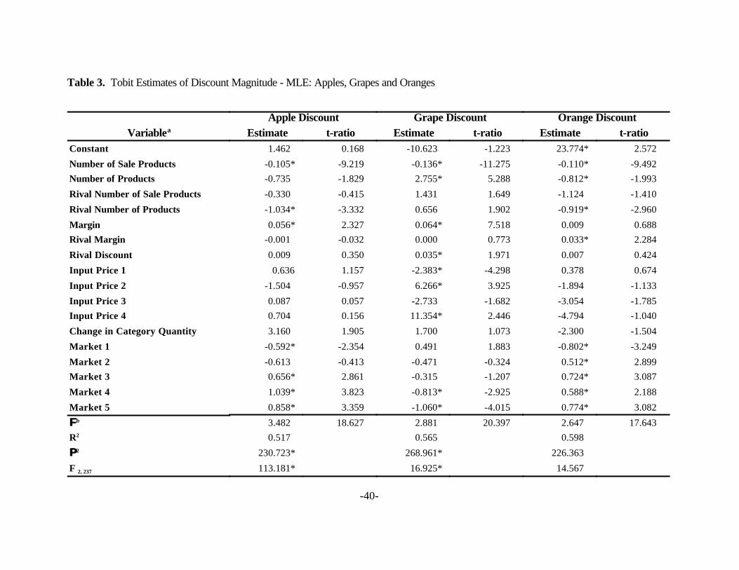
-40-

Table 3. Tobit Estimates of Discount Magnitude - MLE: Apples, Grapes and Oranges

Apple Discount Grape Discount Orange DiscountVariablea Estimate t-ratio Estimate t-ratio Estimate t-ratio

Constant 1.462 0.168 -10.623 -1.223 23.774* 2.572

Number of Sale Products -0.105* -9.219 -0.136* -11.275 -0.110* -9.492Number of Products -0.735 -1.829 2.755* 5.288 -0.812* -1.993

Rival Number of Sale Products -0.330 -0.415 1.431 1.649 -1.124 -1.410

Rival Number of Products -1.034* -3.332 0.656 1.902 -0.919* -2.960

Margin 0.056* 2.327 0.064* 7.518 0.009 0.688Rival Margin -0.001 -0.032 0.000 0.773 0.033* 2.284

Rival Discount 0.009 0.350 0.035* 1.971 0.007 0.424

Input Price 1 0.636 1.157 -2.383* -4.298 0.378 0.674

Input Price 2 -1.504 -0.957 6.266* 3.925 -1.894 -1.133

Input Price 3 0.087 0.057 -2.733 -1.682 -3.054 -1.785Input Price 4 0.704 0.156 11.354* 2.446 -4.794 -1.040

Change in Category Quantity 3.160 1.905 1.700 1.073 -2.300 -1.504

Market 1 -0.592* -2.354 0.491 1.883 -0.802* -3.249

Market 2 -0.613 -0.413 -0.471 -0.324 0.512* 2.899Market 3 0.656* 2.861 -0.315 -1.207 0.724* 3.087

Market 4 1.039* 3.823 -0.813* -2.925 0.588* 2.188

Market 5 0.858* 3.359 -1.060* -4.015 0.774* 3.082

FFb 3.482 18.627 2.881 20.397 2.647 17.643R2 0.517 0.565 0.598

PP2 230.723* 268.961* 226.363

F 2, 237 113.181* 16.925* 14.567

-41-

a Estimates are obtained using a two-stage, sample selection procedure with E[d* | s = 1] = $$ ’z + DF8 where d is the size of the price discount, s is a binaryindicator of a sale’s occurrence, 8 = N / M is the inverse Mill’s ratio calculated from the first-stage Probit equation, F is the standard deviation of the second-stage regression and D is the correlation between Probit and regression residuals.

b The P2 value is a likelihood-ratio test statistic comparing the estimated to a null model wherein all but the constant are restricted to zero. The critical value at 22degrees of freedom and a 5% level of significance is 32.67. The critical F value with 2 and 237 degrees of freedom at 5% is 3.00.

-42-

Table 4. SURE - LES Estimates of Category Promotion Impact: 1998 - 1999 Six Market ScannerData

Variable Estimate t-ratio

Own Pricea -0.070* -1.991

Rival Price 0.012* 26.201

Total Market Expenditure 0.568* 22.872

Number of Products -0.050 -1.462

Number of Sale Products 0.095* 5.192

Rival Products -0.100* -2.507

Rival Sale Products -0.003 -0.320

Own Discount 0.035* 4.573

Own Margin 0.046 1.431

Rival Discount -0.067 -1.434

Rival Margin 1.241* 26.124

R2 0.897

F 0.05, 16, 2043 1,116.400

a A single asterisk indicates significance at a 5% level. Table entries represent elasticities calculated at samplemeans. Other variables in model, for which elasticities are not relevant so are not presented, are: (1) anautoregressive term in category expenditures, and (2) five market-dummy variables.

-43-

Table 5. SURE - LAIDS Model Elasticity Estimates of Product-Level Promotion Impacts: 1998 -1999 Six Market Scanner Data

Product

Apples Grapes Oranges

Variable Non-Sale

Sale Non-Sale

Sale Non-Sale

Sale

Apple Price -1.071*(-56.421)

0.135*(3.277)

0.054*(2.158)

0.063*(1.986)

-1.292*(-44.055)

-2.968*(-56.250)

Apple Sale Price0.021*(2.953)

-0.956*(-30.942)

-0.032*(-3.122)

0.009(0.571)

-0.081*(-5.697)

-0.074*(-2.929)

Grape Price0.049*(3.400)

-0.088*(-2.520)

-1.055*(-36.039)

0.023(1.294)

-0.391*(-18.714)

-0.972*(-26.740)

Grape Sale Price0.038*(3.023)

0.037(1.069)

-0.038*(-2.465)

-1.155*(-32.494)

-0.175*(-7.015)

-0.388*(-8.619)

Orange Price-0.009

(-1.024)-0.076*(-2.919)

0.018(1.495)

0.004(0.224)

-1.022*(-36.654)

-0.432*(-8.850)

Orange Sale Price0.013

(1.908)0.012

(0.646)0.016

(1.393)0.008

(0.427)-0.073*(-3.719)

-0.113*(-28.809)

Category Expenditure0.959*

(160.533)0.936*

(67.638)1.021*

(146.788)1.048*

(75.012)0.929

(1.774)0.213*(7.905)

Number of Products0.022

(1.293)-0.124*(-3.139)

0.112*(3.122)

-0.045(-1.102)

0.051(0.026)

-0.506*(-2.267)

Number of SaleProducts

0.065*(2.515)

1.177(1.417)

0.341*(2.841)

-0.051*(-2.263)

0.900(1.789)

0.460(0.143)

Rival Products0.019*(2.750)

0.000(-0.032)

-0.020(-1.388)

-0.018(-1.093)

-0.077(-1.070)

0.772(0.433)

Rival Sale Products-0.017

(-1.062)0.104*(3.005)

0.018(0.575)

0.029(0.787)

-0.013(-1.350)

0.014(0.300)

Discount Magnitude-0.015

(-1.891)0.002*(2.857)

-0.002*(-2.557)

0.032*(3.667)

-0.001*(-3.843)

0.017*(4.200)

R2 0.736 0.776 0.551 0.596 0.846 0.675

F 438.832* 545.991* 193.525* 232.934* 867.841* 289.712

D.W. 2.644 2.359 2.779 2.412 2.359 2.188

a A single asterisk indicates significance at a 5% level. Values in parentheses are t-ratios. All models also include anautoregressive term in each product’s market share.