price determinants of the european carbon market and ... · price determinants on the european...
TRANSCRIPT

Price Determinants of the European Carbon Market and Interactions with Energy Markets
CLIMATE CHANGE
11/2012


Price Determinants of the European Carbon Market and Interactions with Energy Markets
by
Katja Schumacher Johanna Cludius Felix Matthes Öko-Institut
Jochen Diekmann Aleksandar Zaklan DIW Berlin
Joachim Schleich Fraunhofer-Institut für System- und Innovationsforschung, Karlsruhe
On behalf of the German Federal Environment Agency
UMWELTBUNDESAMT
| CLIMATE CHANGE | 11/2012
ENVIRONMENTAL RESEARCH OF THE GERMAN FEDERAL MINISTRY OF THE ENVIRONMENT, NATURE CONSERVATION AND NUCLEAR SAFETY
Project-no. (FKZ) 3709 41 503 Report-no. (UBA-FB) 001626/E

This publication is only available online. It can be downloaded from http://www.uba.de/uba-info-medien-e/4300.html.
The contents of this publication do not necessarily reflect the official opinions.
ISSN 1862-4359
Study performed by: Deutsches Institut für Wirtschaftsforschung (DIW) Öko-Institut Mohrenstraße 58 Schicklerstraße 5-7 10117 Berlin 10179 Berlin
Fraunhofer Institut für System- und Innovationsforschung ISI Breslauer Straße 48 76139 Karlsruhe
Study completed in: June 2011
Publisher: Federal Environment Agency (Umweltbundesamt) Wörlitzer Platz 1 06844 Dessau-Roßlau Germany Phone: +49-340-2103-0 Fax: +49-340-2103 2285 Email: [email protected] Internet: http://www.umweltbundesamt.de
http://fuer-mensch-und-umwelt.de/
Edited by: Section E 2.3 Reports, National Allocation Plan, Reserve Management Frank Gagelmann
Dessau-Roßlau, June 2012

Abstract
This report explores the determinants of short run price movements in the carbon market and their interaction with energy markets, in particular with the electricity market. Focusing on Phase 2 of the EU ETS we conduct econometric time series analysis based on continental EU and UK market data. Our findings suggest that market fundamentals have a dominant effect on the EUA price, but that non-fundamental factors may also play a role. We further found that the electricity price has a significant positive impact on the carbon price in the short run.

Price Determinants on the European Carbon Market and Interactions with Energy Markets
I
Table of Contents
List of Figures
List of Tables
List of Abbreviations
1 Introduction ........................................................................................................................................ 1
2 Descriptive Analysis ........................................................................................................................... 3
2.1 Carbon Prices .............................................................................................................................. 3
2.2 Energy Prices ............................................................................................................................... 4
2.3 Switching Price ........................................................................................................................... 4
2.4 Economic Activity ....................................................................................................................... 6
2.5 Weather Data .............................................................................................................................. 7
2.6 Overview of Relevant Variables ............................................................................................... 7
3 Model Specification ........................................................................................................................... 9
4 Methodology ................................................................................................................................... 11
5 Results ............................................................................................................................................... 13
5.1 Stationarity and Causality Tests ............................................................................................ 13
5.2 Carbon Price Equation ........................................................................................................... 13
5.3 Electricity Price Equation ....................................................................................................... 16
6 Extensions ........................................................................................................................................ 18
6.1 Spot Electricity Prices .............................................................................................................. 18
6.2 Peak Electricity Prices ............................................................................................................. 19
6.3 Relative Differences (Log-Returns) vs. Absolute Differences ............................................. 20
6.4 Analysis Using Data for the UK ............................................................................................. 21
7 Summary and Conclusion ............................................................................................................. 26
8 Data Sources .................................................................................................................................... 28
9 References ........................................................................................................................................ 29
Appendix A: Results of ADF Tests ......................................................................................................... 30
Appendix B: Granger Causality Tests ................................................................................................... 32
Appendix C: Literature Overview ......................................................................................................... 33

Price Determinants on the European Carbon Market and Interactions with Energy Markets
II
List of Figures
Fig. 1 Spot and Future prices of EUAs 2005-2010 (EEX) .................................................................. 3
Fig. 2 Development of EUA Phase 2 Future, Gas Future (Dutch price until 30/06/2007; German price from 01/07/2010), Coal Future and Base Electricity Future 01/01/2007-31/07/2010 (EEX, Energate, McCloskey) ............................................... 4
Fig. 3 EUA price (future year ahead) and switching price 2007-2010 (EEX, Energate, McCloskey, authors’ own calculations) ................................................................................... 6
Fig. 4 STOXX Euro 600 Index and EUA Futures (future year ahead) 2007-2010 (STOXX, EEX) ............................................................................................................................... 7
Fig. 5 EUA, electricity and energy prices on the continental and UK market (EEX, Energate, ICE, McCloskey) ...................................................................................................... 22
Fig. 6 Switching price: Continental Europe vs. UK (EEX, ICE, McCloskey, authors’ own calculations) ............................................................................................................................. 23
Fig. 7 Development of CO2 prices and their log-returns over time ............................................ 31

Price Determinants on the European Carbon Market and Interactions with Energy Markets
III
List of Tables
Table 1 Parameters for calculating the switching price .................................................................... 5
Table 2 Overview of relevant variables ................................................................................................. 8
Table 3 Expected signs of the coefficients in the carbon price equation .................................... 14
Table 4 Regression results for EUA price equations ........................................................................ 14
Table 5 Expected signs of the coefficients in the electricity price equation ............................... 16
Table 6 Regression results for the electricity price equation using single equation OLS and IV procedures ................................................................................................................... 17
Table 7 Regression results for the (base) spot electricity price equation ..................................... 18
Table 8 Regression results for the EUA equation using base or peak electricity prices as explanatory variable ............................................................................................................... 19
Table 9 Regression results for the base or peak electricity price equations ................................ 19
Table 10 EUA equation in log-returns vs. differences ........................................................................ 20
Table 11 Electricity equation in log-returns vs. differences .............................................................. 21
Table 12 Results for the carbon price equation with continental vs. UK electricity and gas prices .................................................................................................................................. 23
Table 13 Results for the electricity price equation with continental vs. UK electricity and gas prices .................................................................................................................................. 24
Table 14 Results for the carbon price equation including continental and UK electricity and gas prices .......................................................................................................................... 24
Table 15 Results of Augmented Dickey-Fuller Test on time series in levels ................................... 30
Table 16 Results of Augmented Dickey-Fuller Test on log-returns .................................................. 30
Table 17 Results of Granger Causality Tests ........................................................................................ 32

Price Determinants on the European Carbon Market and Interactions with Energy Markets
IV
List of Abbreviations
ADF Augmented Dickey Fuller Test
CER Certified Emission Reduction
CO2 Carbon Dioxide
DWD Deutscher Wetterdienst (German Meteorological Service)
ECM Error Correction Model
EEX European Energy Exchange
ERU Emission Reduction Unit
EU European Union
EUA European Union Allowance
EU ETS European Emissions Trading Scheme
ET Emissions Trading
ICE Intercontinental Exchange
IV Instrumental Variable
MWh Megawatt hour
TWh Terawatt hour
UK United Kingdom
VAR Vector Autoregressive
Price Determinants on the European Carbon Market and Interactions with Energy Markets
1
1 Introduction
Since the launch of the European Emissions Trading Scheme (EU ETS), there has been a growing interest in explaining the functioning of the carbon market. An increasing number of empirical studies have started to analyse the determinants of the price of allowances (EUAs) as well as the interrelations of the carbon market with energy markets. While the supply of EUAs is largely fixed – via emission caps of National Allocation Plans in Phase 1 (2005-2007) and Phase 2 (2008-2012) or from provisions in the modified EU ETS Directive from Phase 3 onwards – the demand for EUAs depends on a large set of variables related to the supply and demand of energy. These may include economic activity in EU ETS sectors, fuel prices, electricity prices, prices of “offsets” (ERUs, CERs), weather conditions (rainfall, wind speed or temperatures) as well as political and institutional factors (see Alberola et al., 2008; Keppler and Mansanet-Bataller, 2010; Fell, 2010; Hintermann, 2010). Besides current circumstances, known and expected future conditions may also affect currently observed carbon prices. Further, long-run and short-run effects need to be distinguished.
Empirical analyses can contribute to the assessment of the carbon market’s efficiency. The EU ETS operates by setting a cap on CO2 emissions, which generates a price that reflects the scarcity in the market. Only if a reliable and significant scarcity signal is generated, can the carbon market stimulate emissions reductions and investment decisions for sustainable structural change. The efficiency of the carbon market can at least in part be assessed on the basis of the development of the carbon price. The main question is whether the carbon price does indeed represent an effective scarcity signal and whether it is largely driven by market fundamentals (e.g. Rickels et al., 2010).
From a policy perspective, the relation between power and EUA prices is of particular interest since windfall profits and competitiveness effects depend on the extent to which carbon costs translate into higher power prices. It has been shown that the price of carbon is passed on to consumers in the form of higher electricity prices, but results from empirical analyses differ as to whether electricity prices also have a short term influence on CO2 prices. While Keppler and Mansanet-Bataller (2010) find that electricity prices influence the price of EUAs, Bunn and Fezzi (2007) reject this effect (for the UK market). Most studies, however, do not test whether power prices affect CO2 allowance prices and assume that this is not the case.
With the exception of Fell (2010),1 empirical findings suggest that fuel prices are the most important drivers of carbon prices, as fuel switching from coal to natural gas provides a short-term opportunity to reduce CO2 emissions for power generators (Bunn and Fezzi, 2007; Convery and Redmond, 2007; Mansanet-Bataller et al., 2007; Alberola et al., 2008; Frunza et al., 2010; Keppler and Mansanet-Bataller, 2010).
Researchers employ different estimation approaches depending on the research question and data at hand. Model specification is typically ad hoc (without economic foundation); only
1 Fell (2010) does not find a reaction of the EUA price to energy prices, but rather to the lagged EUA price (in
differences, lag 1), degree days and dummies for Phase 1 and 2.
Price Determinants on the European Carbon Market and Interactions with Energy Markets
2
Hintermann (2010) develops an economic model as a basis for subsequent econometric analysis. In terms of regional differences, Fell (2010) analyses the Nordic power market, Bunn and Fezzi (2007) the UK power market and Keppler and Mansanet-Bataller (2007, 2010) the French power market. Since electricity market structure, regulation, and fuel mix differ across regions, conducting separate analyses for different regions seems warranted.
Because of data availability several empirical studies are limited to analysing Phase 1 of the EU ETS (Bunn and Fezzi, 2007; Mansanet-Bataller et al., 2007; Alberola et al., 2008; Seifert et al., 2008, Hintermann 2010), while some studies have covered both Phase 1 and the start of Phase 2 (Frunza et al., 2010; Fell, 2010; Keppler and Mansanet-Bataller, 2010). At the time of writing this paper, only one other study we are aware of (Rickels et al, 2010) provides analysis for a time frame comparable to the one used in this study.2
A separate examination of the two phases seems warranted, as Phase 1 of the EU ETS exhibited features that were distinct from all following phases. First, it was characterised by the uncertainty regarding actual emissions and the information shock following the release of verified emissions in April and May 2006. As a consequence, the spot price for EUAs dropped to nearly 0 in 2007, not least because banking from 2007 was prohibited. However, from the second phase onwards, banking is unrestricted for all years, thereby stabilizing prices and making expectations on future developments potentially more relevant. This trend to a more stable carbon price was confirmed since the start of the second trading period, during which the carbon market has become largely established and professionalised. Therefore, findings from Phase 1 may not hold true for Phase 2 of the EU ETS.
The objective of this report is to analyse determinants of EUA prices with a focus on Phase 2 of the EU ETS and to explain its interactions with energy markets, and in particular with the electricity market. Findings will contribute to a better understanding of EUA price developments and market interactions, give an indication of the efficiency of the EU ETS and also provide a stronger empirical basis for projections.
The main research questions to be addressed in this context are:
1. What factors explain the development of EUA prices?
2. What is the relationship between EUA prices and electricity prices?
The remainder of the paper is structured as follows: Section 2 contains a descriptive analysis of the relevant variables in order to give a first indication of their relationship and as a preliminary to specifying the regression equations. Section 3 specifies our regression equations on the basis of economic rationale. Section 4 contains a discussion of methodological considerations and highlights our approach, taking into account special features of time series data. Section 0 presents regressions results and discusses them. Section 6 presents selected extensions to our basic model so that the insights gained can be put into perspective and as a basis for potential further analysis. Section 7 provides a summary of the results and concludes.
2 See Appendix C for an overview of the literature to date.

Price Determinants on the European Carbon Market and Interactions with Energy Markets
3
2 Descriptive Analysis
In the following the time series data used in our study are presented. We use daily data from 01/01/2007 through 31/07/2010.
2.1 Carbon Prices
The EUA price used in our analysis is the year-ahead future contract as traded on the EEX.3 The delivery date of the year-ahead future is December of the following year.
Fig. 1 Spot and Future prices of EUAs 2005-2010 (EEX)
As can be seen in Fig. 1 future and spot price have been tracking closely. Therefore, taking the price of futures as representative for the EUA price seems justified.4 The following trends can be observed:
In 2005 and 2006, the price of EUA futures for Phase 1 (Per 1) increased to € 30. After the publication of the verified emissions in April/May 2006 the EUA price dropped sharply.
In 2008, the price of EUA futures for Phase 2 (Per 2) approached € 30, but decreased in response to the global financial crisis. In February 2009, EUA prices reached their lowest point (€ 8) and stabilised at about € 15 until mid-2010.
3 Since EUAs are homogenous products (and can be traded at low cost), the prices of EUAs are virtually the same
across different exchanges.
4 Keppler and Mansanet-Bataller (2010) also point out that correlation between spot and future prices for EUAs is
close to 1.
0.00
5.00
10.00
15.00
20.00
25.00
30.00
35.00
01.01.2005 01.01.2006 01.01.2007 01.01.2008 01.01.2009 01.01.2010
Spot (CARBIX)
Future Per 1 (year ahead)
Future Per 2 (2008 or year ahead)
Future Per 3 (2013)

Price Determinants on the European Carbon Market and Interactions with Energy Markets
4
2.2 Energy Prices
The carbon market is closely linked to energy markets. The majority of CO2 emissions in the EU ETS are emitted on the basis of electricity generation. Power plant operators decide on production and abatement activities based on prices for natural gas, hard coal, CO2 and electricity. An important abatement option in the power sector is fuel switching, i.e. increasing power generation from gas-fired power plants and lowering generation from hard coal-fired plants (as the specific CO2 emissions of natural gas-fired power plants are lower than the specific emissions of hard coal-fired power plants). Fig. 2 presents the price development of the most important input factors for electricity generation and the electricity price on the continental market. We consider the baseload electricity year-ahead future and gas year-ahead future as traded on the EEX, as well as year-ahead coal futures, as published by EEX and McCloskey. The following trends can be observed:
Prices for natural gas and hard coal have increased since the beginning of 2007 and peaked in the middle of 2008. During the economic crisis the prices of fossil fuels decreased.
Electricity prices show a similar pattern. Prices have increased since the beginning of 2007 and peaked in the year 2008.
Fig. 2 Development of EUA Phase 2 Future, Gas Future (Dutch price until 30/06/2007; German price from 01/07/2010), Coal Future and Base Electricity Future 01/01/2007-31/07/2010 (EEX, Energate, McCloskey)
2.3 Switching Price
The switching price represents a theoretical carbon price above which electricity producers would profit from switching from coal-fired generation to gas-fired generation. It can be
0
10
20
30
40
50
60
70
80
90
100
01.2007 01.2008 01.2009 01.2010
€/M
Wh
; €/
EU
A;
ind
ex
EEX EUA Y+1
Energate TTF Y+1 and EEX NCG Y+1 (from 01/07/2007)
EEX/ Mc Closkey Coal Y+1
EEX Electricity Base Y+1

Price Determinants on the European Carbon Market and Interactions with Energy Markets
5
calculated taking into account efficiency and emissions intensity of the two types of power plants, the prices of coal and gas and solving for the carbon price.5 The thermal efficiencies of coal and gas are set to 36% and 50% respectively, and are widely used EU industry averages. The emissions factors are set to 0.96 t CO2/MWh for coal and 0.411 t CO2/MWh for natural gas. Hence, using these figures which are also shown in Table 1 the calculation would be:
Table 1 Parameters for calculating the switching price
Coal-fired power plant Gas-fired power plant
Efficiency 0.38 0.5 Emissions intensity factor 0.96 t CO2/MWh 0.411 t CO2/MWh
Source: Point Carbon (by subscription only); http://www.pointcarbon.com/
5 The switching price is the price of carbon at which the clean dark and clean spark spread are equal, i.e. economic
rents of coal-fired and gas-fired power plants are equal when taking into account the cost of carbon (i.e, the value of
the required EUAs). In this equation, the electricity prices (as part of the clean dark and clean spark spread) cancel
each other out. We decided to use only the switching price, and not the clean spreads themselves, because prices of
carbon and electricity linearly enter the calculation of the spreads and could thus cause perfect collinearity, while
this is not the case for the switching price.
411.096.0
38.0/5.0/
coalpricegasprice
priceswitching

Price Determinants on the European Carbon Market and Interactions with Energy Markets
6
Fig. 3 EUA price (future year ahead) and switching price 2007-2010 (EEX, Energate, McCloskey, authors’ own calculations)
Fig. 3 compares the price of EUA futures with the switching price. Accordingly, for most of the time considered, the EUA price was substantially lower than the switching price. Only since the beginning of 2010 has the EUA price approached or exceeded the switching price. However, lower prices for gas rather than higher prices for EUAs are responsible for this development. Fig. 3 also indicates a positive correlation between the switching price and the EUA price. This observation would be consistent with the hypothesis that the switching price is a determinant of the EUA price. In particular, a higher switching price is expected to increase the utilisation of coal-fired power plants, which increases the demand for EUAs and thus leads to a higher EUA price.
2.4 Economic Activity
As a proxy for economic activity in the sectors covered by the EU ETS, we use the STOXX Euro 600 Index.6 Fig. 4 plots the EUA price against this index (divided by 10 for better illustration). As a consequence of the global financial crisis, STOXX Euro 600 Index started falling at the end of 2007/beginning of 2008 and has recovered since the start of 2009.7
6 The STOXX Europe 600 Index is derived from the STOXX Europe Total Market Index (TMI) and is a subset of the
STOXX Global 1800 Index. With a fixed number of 600 components, the STOXX Europe 600 Index represents large,
mid and small capitalisation companies across 18 countries of the European region
(http://www.stoxx.com/indices/index_information.html?symbol=SXXP).
7 In earlier applications the Baltic Dry Index (BDI) was used as a proxy for economic activity in the EU ETS sectors. As
an index of prices of shipping of raw materials it seemed to be relevant for the sectors concerned. However, during
0
10
20
30
40
50
60
70
80
90
01.2007 01.2008 01.2009 01.2010
€/E
UA
; €/
MW
h
EEX EUA PII Y+1
Switching price

Price Determinants on the European Carbon Market and Interactions with Energy Markets
7
Fig. 4 STOXX Euro 600 Index and EUA Futures (future year ahead) 2007-2010 (STOXX, EEX)
2.5 Weather Data
Previous research has shown that weather variables, and in particular unanticipated, extreme weather events and temperature changes (cf. Alberola et al., 2008) influence prices on the carbon market and other energy markets. These variables may affect demand (e.g. heating or air conditioning of homes) and supply (e.g. from hydro power, output of condensing plants, output from windmills or photovoltaic modules). We use historical temperature data from a representative German weather station (Düsseldorf), which is available on the website of the German Meteorological Service (www.dwd.de). On days with average temperatures below 15°C (“heating days”) our variable “heating” is calculated as 20 minus average temperature on that day. On days when the maximum temperature is above 25°C (“cooling days”) our variable “cooling” takes a value of maximum temperature on that day minus 25.8
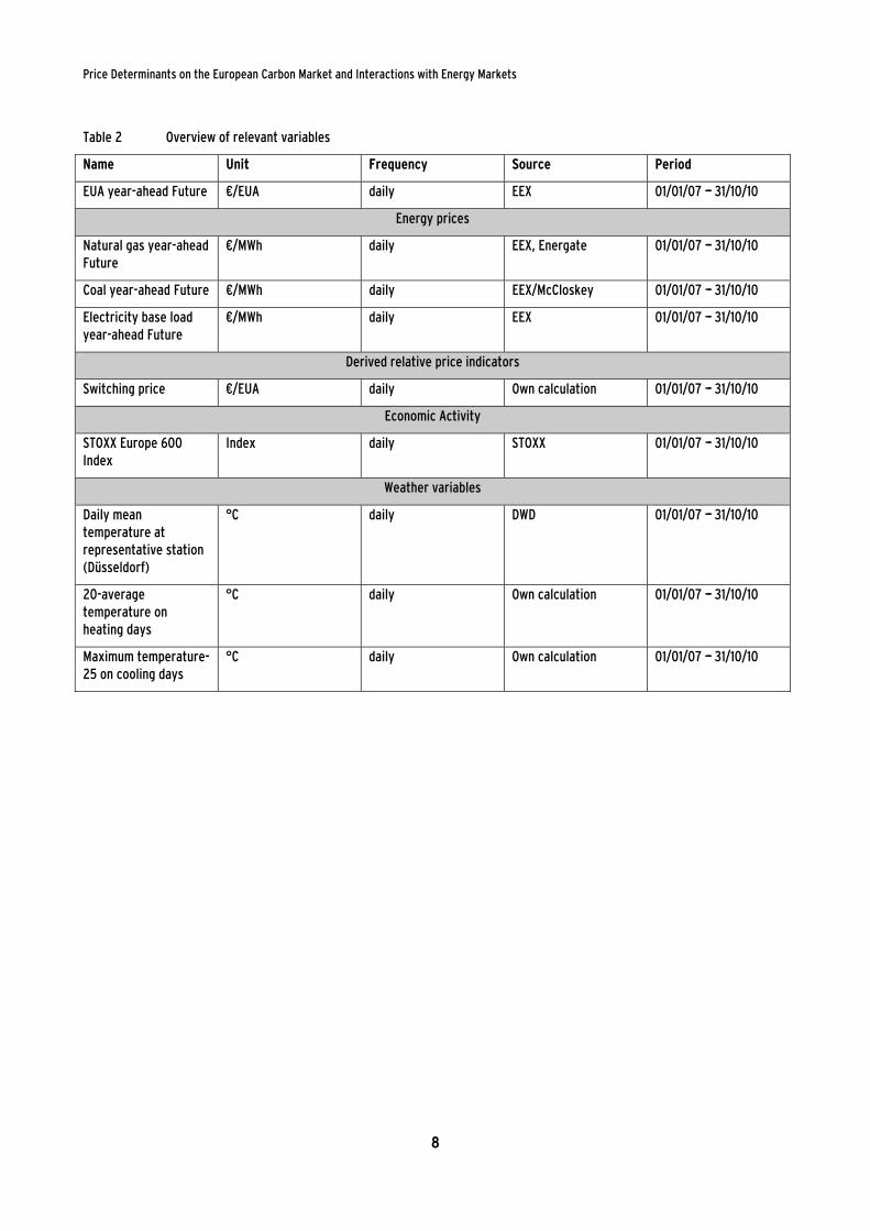
2.6 Overview of Relevant Variables
Table 2 provides an overview of all variables used in our analysis, indicating unit of measurement, frequency, source and time period considered.
the course of the estimation the BDI did not prove significant in the determination of the EUA price, while the
STOXX Europe 600 Index was deemed more appropriate. This might be related to the fact that EUAs are traded on
exchanges and possibly by agents that base their decisions on prominent stock market indices, such as the STOXX
Europe 600.
8 We also experimented with dummies for extreme temperatures. However, this does not alter results.
0
5
10
15
20
25
30
35
40
45
01.2007 07.2007 01.2008 07.2008 01.2009 07.2009 01.2010 07.2010
€/M
Wh
; S
tock
Ma
rke
t In
dex
Eurostoxx600/10
EUA future
Price Determinants on the European Carbon Market and Interactions with Energy Markets
8
Table 2 Overview of relevant variables
Name Unit Frequency Source Period
EUA year-ahead Future €/EUA daily EEX 01/01/07 --- 31/10/10
Energy prices
Natural gas year-ahead Future
€/MWh daily EEX, Energate 01/01/07 --- 31/10/10
Coal year-ahead Future €/MWh daily EEX/McCloskey 01/01/07 --- 31/10/10
Electricity base load year-ahead Future
€/MWh daily EEX 01/01/07 --- 31/10/10
Derived relative price indicators
Switching price €/EUA daily Own calculation 01/01/07 --- 31/10/10
Economic Activity
STOXX Europe 600 Index
Index daily STOXX 01/01/07 --- 31/10/10
Weather variables
Daily mean temperature at representative station (Düsseldorf)
°C daily DWD 01/01/07 --- 31/10/10
20-average temperature on heating days
°C daily Own calculation 01/01/07 --- 31/10/10
Maximum temperature-25 on cooling days
°C daily Own calculation 01/01/07 --- 31/10/10

Price Determinants on the European Carbon Market and Interactions with Energy Markets
9
3 Model Specification
In this section we present the regression equations to be estimated. As noted in the introduction, it is a point of disagreement whether or not the price of electricity affects the price of carbon. From a practical point of view, since both commodities are traded on the same platforms and potentially by the same people, there could well be causality running both ways.
Furthermore, there exist at least two possible theoretical explanations as to why the price of electricity could drive the price of carbon: First, if electricity prices rise as a response to higher electricity demand and if this demand is met by emissions-intensive power stations, the demand and hence the price of EUAs would increase accordingly. Second, if there is market power in the electricity market and hence economic rents can be generated, EUAs can be interpreted as an “entry ticket” to profits. If we assume, for example, that the price of electricity is 60€/MWh, while the price of variable inputs other than EUAs is 50€/MWh, and that a utility needs exactly 1 EUA to generate 1 MWh of electricity, then the utility would be willing to pay 10€/EUA. The higher the price of electricity, the higher the willingness to pay becomes. The prerequisite is, of course, that there is scarcity on the carbon market (cf. also Keppler and Mansanet-Bataller, 2010).
One of the aims of our study is therefore to establish whether or not there is empirical support for the mutual relation between carbon and electricity prices. Of course, our findings would not allow alternative theoretical explanations to be distinguished. We specify four alternative equation systems for the price of EUAs. First, a specification excluding the price of electricity as explanatory variable (Equations 1 and 2) and two equations including the electricity price as explanatory variable (Equations 3 and 4).
In the equations, “gas” refers to the natural gas price in €/MWh, “coal” to the coal price in €/MWh (our applications also included the coal price lagged by one period, taking into account the fact that information might take a day to filter through from the coal to the EUA market, more see Section 5). “Switch” is a variable indicating the level of the EUA price that would induce a fuel switch from coal to gas at the current gas and coal prices.
We alternatively include the prices of coal and gas (Equations 1 and 3) and the switching price (Equations 2 and 4). The fuel prices or the switching price, respectively, are expected to influence the carbon price since they determine the fuel mix of electricity generation, which is the biggest EU ETS sector. “Heating” and “cooling” designate heating and cooling degree days, which are expected to increase the carbon price via higher electricity demand for heating and cooling needs. “Stoxx” is the STOXX Europe 600 Index and captures economic activity in the EU ETS sectors. Finally, “elec” is the price of electricity in €/MWh. One crucial task is to determine whether the coefficients on the electricity price ( e and e) are non-zero.

Price Determinants on the European Carbon Market and Interactions with Energy Markets
10
Equation 5 then addresses the factors determining the electricity price.
In this equation, the EUA price is included because it represents production costs to electricity producers - at least opportunity costs (if EUAs are allocated free of charge). The prices of fuels are production costs for the electricity industry, “stoxx” captures economic development and therefore the demand for electricity, which in turn influences the price. “Heating” and “cooling” also potentially determine demand for electricity. The coefficient of the EUA price represents the pass-through effect to electricity prices. Economic theory and findings from previous studies suggest that CO2 prices have a positive effect on the electricity price (Mansanet-Bataller et al., 2007; Alberola et al., 2008; Fell, 2010;), i.e. we expect α1>0.

Price Determinants on the European Carbon Market and Interactions with Energy Markets
11
4 Methodology
Econometric time series analysis will be applied to assess the relationship between dependent and explanatory variables. When estimating time series models, attention has to be given to the dynamic nature of the variables under consideration. In particular, if variables are governed by a “non-stationary” process,9 Ordinary Least Squares (OLS) estimation procedures may lead to “spurious” regressions and would not be appropriate.10 This means that two variables may show a mathematical correlation although there is no economic meaning to it; for example, because both variables depend on a common third variable,11 or because they are both trending over time. This common trend or time trend can then be erroneously interpreted as an effect which one variable has on the other, when indeed it is a third variable/trend that is driving the results.
Hence, we first test whether the time series data are non-stationary – i.e. whether they exhibit a so-called “unit root” – by conducting the standard Augmented Dickey Fuller (ADF) test. If both the dependent and an explanatory variable are integrated of the same order, the time series of the dependent and explanatory variables can be co-integrated. Co-integration (of the same order) implies that the two integrated time series drift together and a long-run (“equilibrium”) relationship may be assumed. An example are trajectories of certain primary energy prices, e.g. oil and gas, which are partially substitutable and simultaneously determined by the global demand for energy. While we acknowledge the fact that cointegration relationships may exist between variables used in this study and discuss how those might impact on our results, we do not formally test for those relationships, as estimation of cointegration relationships and models exceed the scope of this paper.
If variables are found to be non-stationary and integrated (of order one),12 OLS may be applied to the first differences of the dependent and the explanatory variables. First differences are specified as the change from the previous to the current period, i.e. P(t)-P(t-1). We use those differences in log-form, i.e. ln(P(t)-P(t-1)) (cf. Keppler and Mansanet-Bataller, 2010). Using differences, however, comes at the cost of losing information on levels and possible long-run (co-integrating) relation between variables, because it can only be analysed how short-term changes in one variable (e.g. from one day to the next) impact on changes in another variable, rather than looking at longer-term developments of both variables. A vector auto regressive
9 In order to conduct most time series analysis, stationarity has to be assumed, i.e. the probability distribution of the
variable at each point in time is assumed to be identical.
10 This distinction not only has methodological, but also economic implications. For non-stationary processes, shocks
have permanent effects, while they are of transitory nature for stationary processes.
11 A well-known example is the correlation between the number of storks and the number of newborn babies. At
least historically, both were positively correlated in rural areas.
12 The order of integration is a time series concept specifying the number of differences that need to be taken in
order to obtain a stationary series. Integration of order one means that taking first differences is sufficient. Indeed,
most financial time series data is integrated of order one.

Price Determinants on the European Carbon Market and Interactions with Energy Markets
12
(VAR) or error correction model (ECM) could potentially capture short and long-run dynamics (e.g. Alberola et al., 2008; Fell, 2010). Advanced models could also perform the simultaneous estimation of EUA and electricity prices. Those models, however, are beyond the scope of this paper.
We also conduct so-called Granger causality tests to (stationary) time series. Findings from the Granger causality tests will give a first indication of the suitability of our theoretical model specified in Section 3. Rather than testing for a true causal link, Granger causality tests consider the precedence between two (stationary) time series. As argued by Keppler and Mansanet-Bataller (2010, p. 3329f) “testing for prior causalities is particularly important in the present case, given that economic theory allows for different possibilities of causal links between electricity, carbon and gas prices and their further determinants such as weather conditions or stock market evolutions.”
In principle, several approaches for estimating the suggested relationships are conceivable. We follow the approach of estimating the relations specified in log-returns via the Ordinary Least Squares method (OLS). In order to account for the possible bias induced by mutual influence of the carbon and electricity price on each other, we employ Instrumental Variable (IV) regression, which can correct for this problem, if appropriate instruments are available. If the relevant variable can be “instrumented”, we are left with only part of the variable, which is not affected by the mutual causality problem. That is why IV estimation is generally less precise than OLS. However, in case we can only find “invalid” instruments, the “cure may be worse than the disease“. That is, using IV estimation can lead to results that exhibit larger bias than OLS estimation, if no suitable instruments can be found.
While we find a valid instrument for the EUA price in the electricity equation (the stock market index), all variables that were available to us and could potentially have served as instruments for the electricity price in the carbon equation turned out to be inappropriate. This means that while theoretically a more robust and precise way of estimating the carbon equation should be available, practically we were not able to find adequate instruments. Under those circumstances and considering the concerns about IV regression in the presence of “invalid” instruments, we limit our analysis of the EUA price to OLS regression.

Price Determinants on the European Carbon Market and Interactions with Energy Markets
13
5 Results
5.1 Stationarity and Causality Tests
All time series were tested for stationarity, using the Augmented Dickey Fuller (ADF) test. A well documented stylized fact of financial time series data is their non-stationarity13 and, indeed, it emerges that all price variables as well as the stock market index contain a unit root (i.e. they are non-stationary) while the temperature variables are already stationary in levels. In order to render the series stationary, log-returns are taken. An ADF test on the log-returns reveals that they are stationary, meaning that changes of the variables fluctuate around a fixed mean, rather than exhibiting “random walk”. Detailed test results can be found in Appendix A.
As a second step, Granger causality tests were conducted, which present a way of examining the relationship between two variables, especially if one is not sure in which direction the causality runs. It should be kept in mind that Granger causality tests are not able to establish causality in a theoretical sense. The test examines the causality between two variables, only in a sense that a change in one variable precedes a change in the other. In effect, it is tested whether a forecast of the development of one variable can be improved significantly by adding past values of the other variable. Criticism has been expressed about the usefulness of Granger causality tests (cf. Schulze, 2004). The tests may be misleading if the variables of interest involve expectations, i.e. if future values of a variable are important rather than only past values. Simple tests most often consider only bi-variate relationships, while in our case several variables are likely to interact. Finally, “Granger causality” does not provide insights about the “strength” of the relationships, i.e. about the relevance in an economic sense. The latter can be analysed via appropriate regression analysis.
Keeping this criticism of Granger causality tests in mind, we find that gas and coal Granger cause the EUA price, while the switching price and economic activity do not seem to do so. The most interesting finding is that there seems to be mutual causality between the EUA and the electricity price.
5.2 Carbon Price Equation
We first estimate the four carbon price equations. Table 3 summarises the ex-ante expected signs of the coefficients. An increase in the price of gas (coal) leads to a higher (lower) switching price and hence to an increase (decrease) in coal use and a higher (lower) demand for EUAs. Economic activity in industry sectors is captured by the STOXX Europe 600 Index. Higher economic activity is expected to increase the price of carbon. Heating and cooling needs are expected to increase the demand for, and thus the price of, EUAs.
13 This non-stationarity property is related to the fact that most of financial time series data exhibit “random walk”
behaviour.

Price Determinants on the European Carbon Market and Interactions with Energy Markets
14
Table 3 Expected signs of the coefficients in the carbon price equation
Variable Expected sign
Gas +
Coal -
Switching price +
Stoxx +
Heating/cooling +
As noted above, the apparent mutual causality between carbon and electricity prices is a concern. Hence several instruments for the price of electricity were tested, but this did not produce satisfying results. Therefore, we first present OLS results for the different specifications. When interpreting the results, it should be kept in mind that the mutual causality between carbon and electricity prices might introduce a bias.14 Table 4 shows regression results for the four carbon equations specified in Section 3.
Table 4 Regression results for EUA price equations
Without electricity With electricity
1: Fuels 2: Switch 3: Fuels 4: Switch
Electricity 1.1179** (0.1110) 0.9857** (0.0851)
Gas 0.2947** (0.0755) -0.0478 (0.0854)
Coal 0.1928** (0.0562) -0.1151* (0.0589)
Lagged coal -0.0954** (0.0371) -0.1002** (0.0353)
Switch 0.0995** (0.0191) -0.0267 (0.0335)
Stoxx 0.2529** (0.0529) 0.4113** (0.0504) 0.2056** (0.0527) 0.1846** (0.0514)
Heating -0.0002 (0.0001) -0.0002 (0.0001) 0.0000 (0.0001) -0.0001 (0.0001)
Cooling -0.0012 (0.0007) -0.0014 (0.0007) -0.0007 (0.0006) -0.0007 (0.0006)
Constant 0.0017 (0.0012) 0.0019 (0.0012) 0.0007 (0.0011) 0.0007 (0.0011)
No. of observations 852 853 852 853
R-squared 0.2116 0.117 0.3516 0.3397
Green panels indicate ex-ante expected results. Orange panels indicate results contrary to ex-ante expectation.
** indicates significance at the 1% level * indicates significance at the 5% level ( Robust standard errors in parentheses)
Columns 1 and 2 present the results without the electricity price included in the regression equation. The coefficients can be interpreted as elasticities, meaning that a 1% increase of the
14 Arguably, there might not only be interrelations between the price of carbon and electricity, but also between
carbon and gas or coal prices, since they are simultaneously determined on international markets. In practice
though, this bias is likely to be small. Since the European fuel markets are rather small compared to world markets,
the effect of European CO2 prices on world market fuel prices should be negligible.

Price Determinants on the European Carbon Market and Interactions with Energy Markets
15
gas price will, when all else remains equal, increase the EUA price by 0.29% and accordingly for the other parameters.15 The coal price lagged by one period is included in the model, as it proved significant in explaining the EUA price (including lagged values of all other variables – or further lags of the coal price - did not alter results). The reasoning behind this fact may well be that the market for coal is not as established as the market for gas and that signals from the coal price might take a day to filter through to the carbon market.16
The positive coefficient on the gas and the switching price are as expected; however, the positive coefficient of the coal price is surprising. The lagged coal price, however, has a negative effect on the EUA price as expected. This is consistent with the assumption that the information from the market for coal takes longer to filter through to the EUA market. The European stock market index has the positive significant effect as expected while the temperature variables are insignificant across all specifications.
Turning to the specification including the price of electricity (columns 3 and 4), it can be observed that the coefficients of some variables are altered: The contemporaneous effect of coal is now significant and negative, the gas price and the switching price are negative (although insignificant, i.e. not necessarily different from zero) while the stock market index retains its significant positive influence. The coefficient of the electricity price is large and highly significant, indicating that the electricity price does indeed play a role in the formation of the carbon price (at least in the short term). One explanation for this could be that traders on the EUA market observe the electricity market for guidance on price development. Furthermore, as outlined in Section 3, heightened demand for electricity, if met by emissions-intensive plants, could also drive up demand and the prices of EUAs. As explained above, if there is market power in the electricity market and hence economic rents can be generated, EUAs can be interpreted as an “entry ticket” to profits. The prerequisite is, of course, that there is scarcity on the carbon market (Keppler and Mansanet-Bataller, 2010).
As noted above, it might be important to include additional lagged variables in the regression equations as the carbon price could take a while to adjust to changes in the other variables. However, since we are working with growth rates, lagged variables should be less important
15 If a model is specified in log-returns, the coefficients should be interpreted as constant elasticities. This means,
however, that pass-through rates depend on the level of prices and are not constant. As we expect pass-through rates
to be constant in reality (cost component), a specification in log-returns can be viewed as a good approximation for
small changes. See below for a numeric example.
16 The lagged value of the coal price is included additionally to the contemporaneous coal price, as both current and
day-before prices significantly influence the price of carbon. If only one of those prices were included one might
very well capture some of the effect of the other, which would bias the estimate and make disentangling effects of
prices from different points in time impossible. The two prices are likely to exhibit some level of collinearity.
However, this will always be the case when working with similar variables. Furthermore, multicollinearity does not
impact the point estimations of coefficients, but only the precision they are estimated with, i.e. estimation of
significant coefficients becomes impossible. As both variables are significant in our case, multicollinearity does not
seem to be a problem at this point.

Price Determinants on the European Carbon Market and Interactions with Energy Markets
16
than if we were working with levels. And indeed, in alternative specifications with additional lags of all variables, only the first lag of coal shows up as a significant influence on the price of carbon.17
Once a model is specified, it is still necessary to determine whether statistical inference (i.e. results of hypothesis testing via p-values) can be trusted. This depends on the standard errors of the regression “behaving correctly”. In particular, it is assumed that their variance is constant (no heteroscedasticity) and that they are uncorrelated over time (no autocorrelation). Heteroscedasticity and autocorrelation do not lead to biased coefficient estimates, but they may lead to erroneous statistical inference, i.e. hypothesis tests determining the validity of our estimates. That is why our regressions were carried out using those standard errors that are robust to heteroskedasticity and, where possible, autocorrelation.18
5.3 Electricity Price Equation
We now turn to the estimation of the electricity equation as specified in Section 3. Table 5 details the signs of the coefficients expected ex-ante.
Table 5 Expected signs of the coefficients in the electricity price equation
Expected sign
Gas +
Coal +
EUA +
Stoxx + ( used as instrument in IV regression)
Heating/cooling +
We present both OLS results and, in order to account for possible simultaneous determination of electricity and carbon prices, the results of an Instrumental Variable (IV) regression whereby
17 Naturally, increasing the number of explanatory variables by including an ever greater number of lags would
always increase the explanatory power of an econometric model, even if only marginally. At the same time, the
more variables we include, the less exact our estimation becomes as the model has to estimate more coefficients
with the same amount of observations, i.e. degrees of freedom are lost. In order to select a model with an adequate
lag structure, so-called information criteria can be employed. These test statistics decrease with a better model fit
while they increase when more variables are included, thus “punishing” the excessive use of explanatory variables.
In our case, the information criteria favour the above model in which only the first lag of coal is included (and no
additional lags of any other variable).
18 This “robustification” of standard errors is common practice in the literature. It is used even if one only suspects
that standard errors might not behave correctly, as such it is in the spirit of “better safe than sorry,” i.e. losing some
efficiency of estimation, but being able to trust standard error estimates.

Price Determinants on the European Carbon Market and Interactions with Energy Markets
17
the price of carbon is instrumented by the stock market index.19 As can be seen from Table 6, both procedures lead to similar results. This points to the robustness of our estimates.
Table 6 Regression results for the electricity price equation using single equation OLS and IV procedures
OLS IV
EUA 0.1589** (0.0160) 0.1673 (0.1047)
Gas 0.2595** (0.0418) 0.2570** (0.0525)
Coal 0.2448** (0.0216) 0.2432** (0.0435)
Lagged coal 0.0194 (0.0140) 0.0202 (0.0202)
Stoxx 0.0021 (0.0215)
Heating -0.0001* (0.0000) -0.0001* (0.0000)
Cooling -0.0002 (0.0002) -0.0002 (0.0002)
Constant 0.0006 (0.0004) 0.0006 (0.0004)
No. of observations 852 852
R-squared 0.7078 0.7076
Green panels indicate ex-ante expected results. Orange panels indicate results contrary to ex-ante expectation.
** indicates significance at the 1% level * indicates significance at the 5% level ( Robust standard errors in parentheses)
As expected, both gas and coal prices have a positive influence on the price of electricity and are highly significant. The stock market index and the indicator for cooling on hot days, however, are insignificant. The indicator for heating on cold days is significant and negative (which is surprising since heating demand should drive up the price of electricity); however, this coefficient is very small in magnitude.
Results of the IV regression are very similar, with coefficients exhibiting larger standard errors, which was to be expected.20 Results imply that a 1% increase in the price of carbon increases the electricity price by 0.16%. For example, if the carbon price increases from € 15 to € 16 (by 6.7 %), an electricity price of 50 €/MWh is expected to increase by 0.50 €/MWh (1 %). This estimate represents the lower end of common estimations predicting a price increase of between 0.50 €/MWh and 1 €/MWh per €/EUA.21
19 As explained in Section 4, using instruments, we can separate the part of the variable suitable for the regression
from the other part, which might introduce a bias.
20 As IV regressions only use part of the variable for estimation, the process is less precise, i.e. more observations
would be necessary to generate the same level of precision. Therefore, larger standard errors were to be expected.
21 E.g. Sijm et al. (2006) estimate pass-through rates for Germany and the Netherlands of between 60% and 100%, but
state that the true value may be underestimated.
Price Determinants on the European Carbon Market and Interactions with Energy Markets
18
6 Extensions
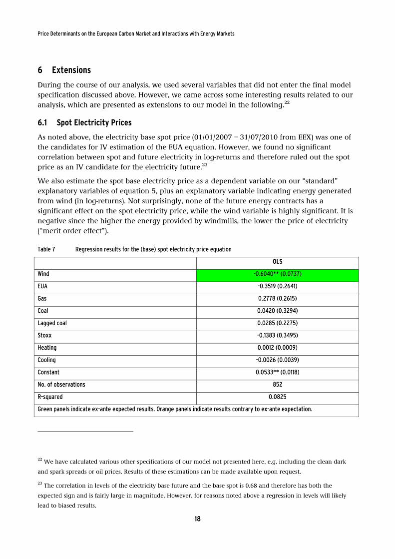
During the course of our analysis, we used several variables that did not enter the final model specification discussed above. However, we came across some interesting results related to our analysis, which are presented as extensions to our model in the following.22
6.1 Spot Electricity Prices
As noted above, the electricity base spot price (01/01/2007 – 31/07/2010 from EEX) was one of the candidates for IV estimation of the EUA equation. However, we found no significant correlation between spot and future electricity in log-returns and therefore ruled out the spot price as an IV candidate for the electricity future.23
We also estimate the spot base electricity price as a dependent variable on our “standard” explanatory variables of equation 5, plus an explanatory variable indicating energy generated from wind (in log-returns). Not surprisingly, none of the future energy contracts has a significant effect on the spot electricity price, while the wind variable is highly significant. It is negative since the higher the energy provided by windmills, the lower the price of electricity (“merit order effect”).
Table 7 Regression results for the (base) spot electricity price equation
OLS
Wind -0.6040** (0.0737)
EUA -0.3519 (0.2641)
Gas 0.2778 (0.2615)
Coal 0.0420 (0.3294)
Lagged coal 0.0285 (0.2275)
Stoxx -0.1383 (0.3495)
Heating 0.0012 (0.0009)
Cooling -0.0026 (0.0039)
Constant 0.0533** (0.0118)
No. of observations 852
R-squared 0.0825
Green panels indicate ex-ante expected results. Orange panels indicate results contrary to ex-ante expectation.
22 We have calculated various other specifications of our model not presented here, e.g. including the clean dark
and spark spreads or oil prices. Results of these estimations can be made available upon request.
23 The correlation in levels of the electricity base future and the base spot is 0.68 and therefore has both the
expected sign and is fairly large in magnitude. However, for reasons noted above a regression in levels will likely
lead to biased results.

Price Determinants on the European Carbon Market and Interactions with Energy Markets
19
OLS
** indicates significance at the 1% level * indicates significance at the 5% level ( Robust standard errors in parentheses)
6.2 Peak Electricity Prices
In a next step, we examined how far our results changed when taking future peak-load (01/01/2007 – 31/07/2010 from EEX) rather than base-load electricity prices as the basis for our analysis.
Table 8 Regression results for the EUA equation using base or peak electricity prices as explanatory variable
With Base Electricity Price With Peak Electricity Price
Fuels Switch Fuels Switch
Electricity 1.1179** (0.1110) 0.9857** (0.0851) 0.7132** (0.1362) 0.8599** (0.1013)
Gas -0.0478 (0.0854) 0.0452 (0.0813)
Coal -0.1151* (0.0589) 0.0552 (0.0620)
Lagged coal -0.1002** (0.0353) -0.0893* (0.0354)
Switch -0.0267 (0.0335) -0.0265 (0.0324)
Stoxx 0.2056** (0.0527) 0.1846** (0.0514) 0.2362** (0.0545) 0.2515** (0.0523)
Heating 0.0000 (0.0001) -0.0001 (0.0001) -0.0001 (0.0001) -0.0001 (0.0001)
Cooling -0.0007 (0.0006) -0.0007 (0.0006) -0.0009 (0.0007) -0.0009 (0.0006)
Constant 0.0007 (0.0011) 0.0007 (0.0011) 0.0013 (0.0011) 0.0012 (0.0011)
No. of observations 852 853 852 853
R-squared 0.3516 0.3397 0.2712 0.2644
Robust standard errors in parentheses
** indicates significance at the 1% level * indicates significance at the 5% level
Table 8 shows results for the EUA equation using base electricity prices and peak electricity prices, respectively. Again it can be observed that the results are largely similar while the effect that the peak electricity future has on the EUA price is somewhat smaller in magnitude than the effect of the base future.
Table 9 Regression results for the base or peak electricity price equations
Base Peak
EUA 0.1589** (0.0160) 0.1060** (0.0180)
Gas 0.2595** (0.0418) 0.3185** (0.0591)
Coal 0.2448** (0.0216) 0.1725** (0.0199)
Lagged coal 0.0194 (0.0140) 0.0016 (0.0151)
Stoxx 0.0021 (0.0215) -0.0034 (0.0210)
Heating -0.0001* (0.0000) -0.0001 (0.0000)
Cooling -0.0002 (0.0002) -0.0002 (0.0002)

Price Determinants on the European Carbon Market and Interactions with Energy Markets
20
Base Peak
Constant 0.0006 (0.0004) 0.0003 (0.0004)
No. of observations 852 852
R-squared 0.7078 0.6326
Green panels indicate ex-ante expected results. Orange panels indicate results contrary to ex-ante expectation.
** indicates significance at the 1% level * indicates significance at the 5% level ( Robust standard errors in parentheses)
Table 9 reveals that the determinants for the peak-load electricity price are largely similar to those for the base-load price: The effect of the gas price is slightly larger while the effect of the coal price is slightly smaller, which could be expected because gas is the marginal plant for a large share of the peak load hours, in contrast to base load where coal plants dominate as the marginal plant.
6.3 Relative Differences (Log-Returns) vs. Absolute Differences
Running the regressions in absolute differences rather than log-returns should not alter results fundamentally. However, coefficients have to be interpreted differently. While log-returns describe percentage changes, absolute differences describe changes in specific units of measurement. As shown in Table 10, estimating the EUA equation (without electricity prices) in differences qualitatively leads to the same results as using the specification in log-returns, i.e. parameter estimates exhibit the same signs and similar levels of significance.
Table 10 EUA equation in log-returns vs. differences
Log-Returns Differences
Fuels Switch Fuels Switch
Gas 0.2947** (0.0755) 0.2758** (0.0526)
Coal 0.1928** (0.0562) 0.3074** (0.0991)
Lagged Coal -0.0954** (0.0371) -0.1642* (0.0668)
Switch 0.0995** (0.0191) 0.0658** (0.0120)
Stoxx 0.2529** (0.0529) 0.4113** (0.0504) 0.0164** (0.0036) 0.0263** (0.0037)
Heating -0.0002 (0.0001) -0.0002 (0.0001) -0.0025 (0.0020) -0.0028 (0.0021)
Cooling -0.0012 (0.0007) -0.0014 (0.0007) -0.0223 (0.0133) -0.0276 (0.0160)
Constant 0.0017 (0.0012) 0.0019 (0.0012) 0.0265 (0.0230) 0.0335 (0.0248)
No. of observations 852 853 852 853
R-squared 0.2116 0.117 0.2633 0.2013
Green panels indicate ex-ante expected results. Orange panels indicate results contrary to ex-ante expectation.
** indicates significance at the 1% level * indicates significance at the 5% level ( Robust standard errors in parentheses)

Price Determinants on the European Carbon Market and Interactions with Energy Markets
21
Table 11 shows the corresponding comparison for the electricity equation. The effect of the EUA price on the electricity price is 0.52 €/MWh per €/EUA. This confirms the estimate given in section 5.2.24
Table 11 Electricity equation in log-returns vs. differences
Depvar.: Electricity Log-Returns Differences
EUA 0.1589** (0.0160) 0.5249** (0.0505)
Gas 0.2595** (0.0418) 0.6257** (0.0971)
Coal 0.2448** (0.0216) 1.6017** (0.1312)
Lagged coal 0.0194 (0.0140) 0.1040 (0.0908)
Stoxx 0.0021 (0.0215) -0.0015 (0.0045)
Heating -0.0001* (0.0000) -0.0006 (0.0054)
Cooling -0.0002 (0.0002) -0.0224 (0.0127)
Constant 0.0006 (0.0004) -0.0128 (0.0152)
No. of observations 852 852
R-squared 0.7078 0.734
Green panels indicate ex-ante expected results. Orange panels indicate results contrary to ex-ante expectation.
** indicates significance at the 1% level * indicates significance at the 5% level ( Robust standard errors in parentheses)
6.4 Analysis Using Data for the UK
As a final extension to our basic model, we turn to an analysis of the UK market based on the electricity base future and natural gas future as traded on the ICE. The relevant period is again 01/01/2007 – 31/07/2010. Those derivatives are traded in seasons. We depict both the winter and the summer future in our figures, while for our regressions we use the winter future because it does not contain gaps in the data series.
24 One has to keep in mind, however, that while the estimated 0.52 are a constant parameter, the coefficient in
Section 5.2 is dependent on the magnitude of the electricity and EUA prices. For average values this statement holds.

Price Determinants on the European Carbon Market and Interactions with Energy Markets
22
Fig. 5 EUA, electricity and energy prices on the continental and UK market (EEX, Energate, ICE, McCloskey)
Fig. 5 depicts the UK price series against the continental prices. Electricity prices are slightly higher in the UK than on the continental market, but they exhibit a similar pattern. In fact, the correlation between the two prices in levels is 0.98 while the correlation in log-returns is 0.61, which is a first indication that analysis based on British data might lead to similar results as the analysis conducted above. Similarly, the development of British and continental gas futures seems to be very harmonious. Fig. 6 depicts the theoretical switching price on the continental and UK markets. Owing to relatively higher gas prices in the winter season and lower gas prices in the summer, the switching price in the UK is higher in winter and lower in summer than on the continental market.
0
20
40
60
80
100
120
140
01.2007 01.2008 01.2009 01.2010
€/M
Wh
; €/
EU
A;
ind
ex
EUA Y+1UK Electricity Base Winter Y+1UK Electricity Base Summer Y+1EEX Electricity Base Y+1EEX/ Mc Closkey Coal Y+1UK Gas Winter Y+1UK Gas Summer Y+1Continental Gas Y+1

Price Determinants on the European Carbon Market and Interactions with Energy Markets
23
Fig. 6 Switching price: Continental Europe vs. UK (EEX, ICE, McCloskey, authors’ own calculations)
The main rationale for our analysis of data from the UK is to check whether the different fuel mix – i.e. more gas-fired power plants in the UK – would show up in the regressions and whether continental and British power prices might jointly influence the EUA price. Table 12 presents results for the EUA equation, comparing continental data with UK data; the columns 1 and two only differ from columns 3 and 4 with respect to the electricity and gas prices used. Coefficients are similar in terms of direction of the effect and significance; however, the British electricity price seems to have a smaller impact while the British gas price has a larger coefficient compared to the continental data.
Table 12 Results for the carbon price equation with continental vs. UK electricity and gas prices
Continental UK
Without electricity With electricity Without electricity With electricity
Electricity 1.1179** (0.1110) 0.4519** (0.1060)
Gas 0.2947** (0.0755) -0.0478 (0.0854) 0.4709** (0.0552) 0.1213 (0.0947)
Coal 0.1928** (0.0562) -0.1151* (0.0589) 0.1395* (0.0551) 0.1083 (0.0556)
Lagged coal -0.0954** (0.0371) -0.1002** (0.0353) -0.1079** (0.0366) -0.1234** (0.0354)
Stoxx 0.2529** (0.0529) 0.2056** (0.0527) 0.2665** (0.0516) 0.2484** (0.0517)
Heating -0.0002 (0.0001) 0.0000 (0.0001) -0.0001 (0.0001) -0.0001 (0.0001)
Cooling -0.0012 (0.0007) -0.0007 (0.0006) -0.0011 (0.0007) -0.0012 (0.0007)
Constant 0.0017 (0.0012) 0.0007 (0.0011) 0.0015 (0.0012) 0.0014 (0.0012)
No. of observations 852 853 850 837
R-squared 0.21 0.12 0.24 0.27
Green panels indicate ex-ante expected results. Orange panels indicate results contrary to ex-ante expectation.
0
10
20
30
40
50
60
70
80
90
100
01.2007 01.2008 01.2009 01.2010
€/E
UA
EEX EUA PII Y+1Continental SwitchUK Winter SwitchUKSummer Switch

Price Determinants on the European Carbon Market and Interactions with Energy Markets
24
Continental UK
** indicates significance at the 1% level * indicates significance at the 5% level ( Robust standard errors in parentheses)
Table 13 presents results for the electricity equation comparing continental data with UK data. As expected, the gas price has a larger effect on electricity prices in the UK, while the effect of the coal price is smaller. Furthermore, the coefficient of the EUA price is smaller, which reflects that the marginal power producer in the UK is less CO2-intensive than in Germany.
Table 13 Results for the electricity price equation with continental vs. UK electricity and gas prices
Continental UK
EUA 0.1589** (0.0160) 0.0714** (0.0124)
Gas 0.2595** (0.0418) 0.7395** (0.0217)
Coal 0.2448** (0.0216) 0.0518* (0.0245)
Lagged coal 0.0194 (0.0140) 0.0350* (0.0177)
Stoxx 0.0021 (0.0215) 0.0044 (0.0291)
Heating -0.0001* (0.0000)
Cooling -0.0002 (0.0002)
Constant 0.0006 (0.0004) -0.0001 (0.0003)
No. of observations 852 837
R-squared 0.71 0.75
Green panels indicate ex-ante expected results. Orange panels indicate results contrary to ex-ante expectation.
** indicates significance at the 1% level * indicates significance at the 5% level ( Robust standard errors in parentheses)
Finally, Table 14 presents results of a regression which include both continental and British electricity and gas prices. The results indicate that electricity prices on both markets do indeed have a high and significant influence on the prices of EUAs; the influence of the continental market seems to be more pronounced than that of the UK price. This result could be expected since the continental market is larger than the British one.
Table 14 Results for the carbon price equation including continental and UK electricity and gas prices
Depvar.: EUA OLS
Continental elec. 1.0286** (0.1107)
UK elec. 0.3681** (0.0992)
Continental gas -0.2513* (0.1090)
UK gas 0.0990 (0.1205)
Coal -0.1634* (0.0606)
Lagged coal -0.1214** (0.0337)
Stoxx 0.2071** (0.0524)
Constant 0.0002 (0.0007)
No. of observations 837

Price Determinants on the European Carbon Market and Interactions with Energy Markets
25
Depvar.: EUA OLS
R-squared 0.38
Green panels indicate ex-ante expected results. Orange panels indicate results contrary to ex-ante expectation.
** indicates significance at the 1% level * indicates significance at the 5% level ( Robust standard errors in parentheses)

Price Determinants on the European Carbon Market and Interactions with Energy Markets
26
7 Summary and Conclusion
This report explored the determinants of short-run price movements in the carbon market and their interaction with energy markets and the electricity market in particular. We first provided an overview of the research in the field to date, which has predominantly focused on Phase 1 of the EU ETS. Focusing on Phase 2, our analysis extends current knowledge and allows for comparisons across time and regions, i.e. continental EU and UK. More specifically, we presented a descriptive analysis of price developments and specified economically sound regression equations for the EUA price and the electricity price.
Findings of our econometric time series analysis based on continental EU and UK market data suggests that the EUA price reacts to market fundamentals, indicating that the European carbon market is able to effectively reflect relevant information of energy markets for the scarcity of EUAs. In particular, the gas and switching price tend to exhibit the expected positive effect and the coal price the expected negative effect on the price of EUA, while economic activity has a positive effect. The estimated parameters for coal and gas prices as well as economic activity are highly significant and proved to be robust in terms of sensitivity analyses of different model specifications25. The parameters can be interpreted as elasticities, showing the percentage increase in the EUA price for a given 1% increase of the exogenous variable. The coefficients for the gas price and economic activity in the continental market turn out to be in the same range of 0.25 (economic activity) to 0.3 (gas price). This implies that a 1% increase of the price of natural gas, for example, would result in a 0.29% increase of the EUA price. The effect of a change in coal prices is negative and substantially smaller (-0.09). In the specification including the switching price, it shows an elasticity of around 0.1.
Temperature variables and the coefficient on the coal and switching price in some specifications, however, are not according to our expectations. These findings are in line with previous studies, e.g. Rickels et al. (2010) who also find a positive effect of the coal price and insignificant results for their weather variables (see Appendix C for a literature overview). Given the significance of the results for the influence of major market fundamentals, i.e. energy prices and economic activity, we conclude that the EUA price is mainly driven by these factors. However, other, non-fundamental factors, such as availability of reliable information, expectations or speculation on policies or policy implementation, on activities of other market players, on future development of overall economic markets and prices, may also affect the price of EUAs, at least in the short term.
Our findings further imply that the electricity price has a large positive impact on the carbon price in the short run (elasticity of about 1). This may point to market power in the electricity market or, maybe more convincingly, to the fact that additional electricity demand is met by emissions-intensive plants. To account for this potential simultaneity, we employed Instrumental Variable (IV) regression techniques. While we were able to find appropriate instruments for the EUA price, this was not possible for the price of electricity. However, the results for the electricity price equation remained largely similar to standard Ordinary Least
25 See Section 6 for an illustration of some of these different specifications.

Price Determinants on the European Carbon Market and Interactions with Energy Markets
27
Squares (OLS) when estimating an IV regression. The estimates show significant positive effects for an increase of EUA, gas, and coal prices on the electricity price with elasticities of 0.16, 0.26 and 0.25 respectively.
Overall, the analysis presented in this report illustrates that estimating the development of the EUA price is challenging in terms of data availability and methodology. Issues of non-stationarity and interdependency with other markets, in particular the electricity market, need to be properly taken into account. Our analysis based on daily data and relative differences (log-returns) addresses these issues and reveals interesting patterns. By estimating a wide range of models and allowing for different specifications, our analysis offers additional insights into the robustness of the findings.
More specifically, we also present extensions and sensitivity analyses, looking at spot rather than future electricity prices, peak rather than base electricity prices and absolute differences rather than log-returns. In general, results remain robust.
To provide a comparison with other EU markets, we also included a first analysis of UK market data using the same model specification and methodology. The analysis for the UK reveals similar patterns as the analysis for continental Europe and at the same time reflected the different fuel mix of UK electricity generation. The coefficient for the influence of the EUA price on the electricity price, at average prices, is lower in the UK than in Germany due to the lower carbon intensity of the UK fuel mix. As in the continental European market, the analysis for the UK indicates a significant influence of electricity prices on EUA prices.
When interpreting our findings, it should be taken into account that we analyse short-run day-to-day changes in the variables rather than levels, owing to stationarity requirements of the underlying processes. As such, it can give a good indication of the underlying short-run dynamics. As markets react fast in adjusting their prices, usually on a daily basis, such an analysis of short-run dynamics contributes significantly to the understanding of the interaction of markets and the determinants of prices. It therefore adds in a relevant way to the existing literature.
Future research may explore more advanced econometric methods, such as error correction models (ECM) or vector autoregressive (VAR) models to capture both short-run and long-run dynamics. The studies by Fell (2010) and Chevallier (2010) employ such advanced econometric approaches but analyse different markets, i.e. the Nordic markets in the case of Fell and EUA vs. CER markets in the case of Chevallier. They are thus not comparable to our study.26 Improving the understanding of the long-term development of the EU ETS price signal, in addition to the short-term analysis, would be vital for long-term decision-making, such as investment decisions, and for structural change towards a low-carbon economy. Therefore, the price development in the carbon market should continue to be monitored both on the short-term and long-term level.
26 At this point, we are not aware of any study that uses more advanced econometric methods and aims to analyse
questions similar to ours.

Price Determinants on the European Carbon Market and Interactions with Energy Markets
28
8 Data Sources
Deutscher Wetterdienst (DWD)
European Energy Exchange (EEX): Market Data. Power Spot Market. Results Electricity – Market Area Germany/Austria. EPEX Spot Auction, Leipzig
European Energy Exchange (EEX): Market Data. Power Derivatives Market. Results Electricity Phelix Futures. Yearly Futures, Leipzig
European Energy Exchange (EEX): Market Data. EU Emission Allowances. Results EU Emission Allowances - Derivatives Market. Leipzig
European Energy Exchange (EEX): Market Data. EU Emission Allowances. Results EU Emission Allowances - Spot Market, Leipzig
European Energy Exchange (EEX): Market Data. Results Coal Futures – Yearly Futures, Leipzig
European Energy Exchange (EEX): Market Data. Results Natural Gas - Derivatives Market– NCG Futures – Yearly Futures, Leipzig
European Energy Exchange (EEX): Market Data. Results Natural Gas – Derivatives Market – Gaspool Futures – Yearly Futures, Leipzig
Energate: Marktdaten; Price Forward Curves, TTF (Title Transfer Facility), Natural gas yearly Futures in the Netherlands, www.energate.de
Intercontinental Exchange (ICE): Data, End of Day Reports, Daily Volumes for ICE UK Base Electricity Futures (Seasons), www.theice.com
Intercontinental Exchange (ICE): Data, End of Day Reports, Daily Volumes for ICE UK Natural Gas Futures (Seasons), www.theice.com
McCloskey: Coal, Argus McCloskey's Coal Price Index Report, Argus Coal Daily, Coal future with delivery in Rotterdam, API 2, www.mccloskeycoal.com; http://www.argusmedia.com
Point Carbon: Parameters for the Calculation of Clean Dark and Spark Spreads (by subscription only) http://www.pointcarbon.com/news/marketdata/methodology/forward/modeldescriptions/
STOXX: Data Centre, Historical Data, Benchmark Indices, Stoxx Europe 600, SXXP Broad Europe, www.stoxx.com

Price Determinants on the European Carbon Market and Interactions with Energy Markets
29
9 References
Alberola, E., Chevallier, J. and Chèze, B. (2008): Price drivers and structural breaks in European carbon prices 2005-2007. Energy Policy 36, 787-797.
Benz, E. and Trück, S. (2008): Modeling the price dynamics of CO2 emission allowances. Energy Economics 31, 4–15.
Bunn, D. and Fezzi, C. (2007): Interaction of European Carbon Trading and Energy Prices, Fondazione Eni Enrico Mattei Working Paper 123.
Chevallier, J. (2010): EUAs and CERs: Vector Autoregression, Impulse Response Function and Cointegration Analysis, Economics Bulletin 30(1).
Convery, F. and Redmond, L. (2007): Market and Price Developments in the European Union Emissions Trading Scheme. Review of Environmental Economics and Policy, 1 (1), 88-111.
Fell, H. (2010): EU-ETS and Nordic Electricity – A CVAR Analysis. Energy Journal 31(2).
Frunza, M., D.Guegan and Lassoudiere, A. (2010): Dynamic factor analysis of carbon allowances prices – From classic Arbitrage Pricing Theory to Switching Regimes, CES Working Paper 2010.62.
Hintermann, B. (2010): Allowance pirce drivers in the first phase of the EU ETS. Journal of Environmental Economics and Management 59, 43–56.
Kilian, L. (2009): Not all oil price shocks are alike: Disentangling Demand and Supply Shocks in the Crude Oil Market, American Economic Review 99(3), 1053-1069.
Keppler, J. and Mansanet-Bataller, M. (2010): Causalities between CO2, electricity, and other energy variables during phase I and phase II of the EU ETS. Energy Policy 38, 3329 – 3341.
Keppler, J. (2010): The interaction between the EU ETS und European electricity markets. In Ellermann et al. (eds.) Pricing Carbon: The European Emissions Trading Scheme. Cambridge University Press.
Mansanet-Bataller, M., Pardo, A., and Valor, E. (2007): CO2 prices, energy and weather. The Energy Journal 28 (3), 67–86.
Rickels, W., Görlich, D. and Oberst, G. (2010): Explaining European Emission Allowance Price Dynamics: Evidence from Phase II, IfW Working Papers 1650.
Schulze, P.M. (2004): Granger-Kausalitätsprüfung – Eine anwendungsorientierte Darstellung, Institut für Statistik und Ökonometrie, Johannes Gutenberg-Universität Mainz, Arbeitspapier 28.
Seifert, J., Uhrig-Homburg, M. and Wagner, M. (2008): Dynamic behavior of CO2 spot prices. Journal of Environmental Economics and Management 56, 180-194.
Sijm, J., Neuhoff, K. and Chen, Y. (2006): CO2 cost pass through and windfall profits in the power sector. Climate Policy 6.1, 49-72.

Price Determinants on the European Carbon Market and Interactions with Energy Markets
30
Appendix A: Results of ADF Tests
The null hypothesis of the Augmented Dickey-Fuller (ADF) test is that the time series variable contains a unit root (against the alternative hypothesis that the variable was generated by a stationary process). Findings for the variables in levels in Table 15 suggest that all time series, except the temperature variables, are non-stationary. In contrast, for log-returns we reject the null hypothesis of non-stationarity.
Table 15 Results of Augmented Dickey-Fuller Test on time series in levels
Time series Test statistic 1% Critical value Conclusion
EUA year-ahead Future -1.260 -3.430 Fail to reject H0
Natural gas year-ahead Future
-1.082 -3.430 Fail to reject H0
Coal year-ahead Future -1.484 -3.430 Fail to reject H0
Electricity base-load year-ahead Future
-1.149 -3.430 Fail to reject H0
Switching price -1.206 -3.430 Fail to reject H0
STOXX Europe 600 Index -1.261 -3.430 Fail to reject H0
Heating indicator -5.986 -3.430 Reject H0
Cooling indicator -16.567 -3.430 Reject H0
Table 16 Results of Augmented Dickey-Fuller Test on log-returns
Time series Test statistic 1% Critical value Conclusion
EUA year-ahead Future -25.774 -3.430 Reject H0
Natural gas year-ahead Future
-27.495 -3.430 Reject H0
Coal year-ahead Future -28.870 -3.430 Reject H0
Electricity base-load year-ahead Future
-27.603 -3.430 Reject H0
Switching price -29.568 -3.430 Reject H0
STOXX Europe 600 Index -29.545 -3.430 Reject H0
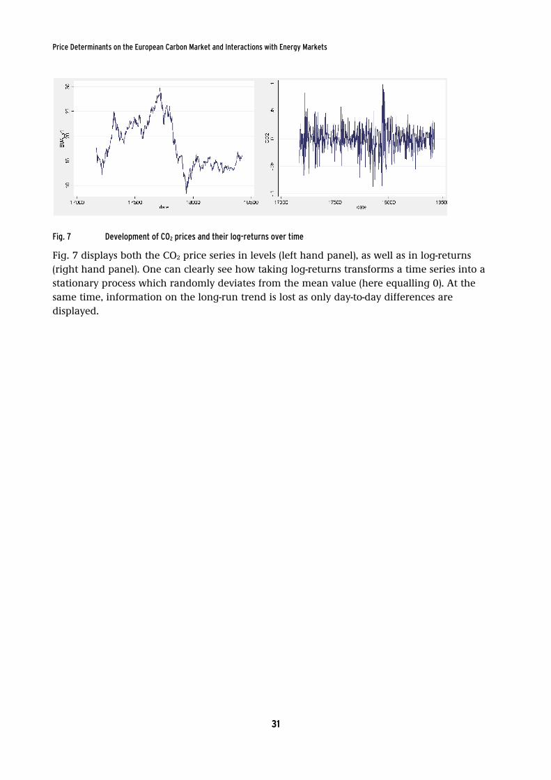
Price Determinants on the European Carbon Market and Interactions with Energy Markets
31
Fig. 7 Development of CO2 prices and their log-returns over time
Fig. 7 displays both the CO2 price series in levels (left hand panel), as well as in log-returns (right hand panel). One can clearly see how taking log-returns transforms a time series into a stationary process which randomly deviates from the mean value (here equalling 0). At the same time, information on the long-run trend is lost as only day-to-day differences are displayed.

Price Determinants on the European Carbon Market and Interactions with Energy Markets
32
Appendix B: Granger Causality Tests
Table 17 details results of the Granger causality test. The null hypothesis states that no Granger causality is present. Hence, for a test statistic that is sufficiently large, the null is rejected and Granger causality assumed.
Table 17 Results of Granger Causality Tests
Null hypothesis for prices T-statistic Probability (p-values) Conclusion
Energy prices
Gas does not Granger cause CO2
9.98 0.01 Reject H0 → Gas causes CO2
Coal does not Granger cause CO2
18.47 0.00 Reject H0 →Coal causes CO2
Switching price does not Granger cause CO2
2.52 0.28 Fail to reject H0 →Switching price does not cause CO2
Economic activity
Stoxx does not Granger cause CO2
5.72 0.06 Fail to reject H0 →Stoxx does not cause CO2
Weather variables
Heating does not Granger cause CO2
2.68 0.26 Fail to reject H0 → Heating does not cause CO2
Cooling does not Granger cause CO2
1.04 0.60 Fail to reject H0 →Cooling does not cause CO2
Electricity prices
Electricity does not Granger cause CO2
20.16 0.00 Reject H0 →Electricity causes CO2
CO2 does not Granger cause electricity
6.15 0.05 Reject H0 →CO2 causes electricity

Price Determinants on the European Carbon Market and Interactions with Energy Markets
33
Appendix C: Literature Overview
PHASE I
Mansanet-Bataller et al. (2007) Alberola et al. (2008) Bunn + Fezzi (2007) Period 2005 Juli 2005 – April 2007 April 2005 – May 2006 Frequency Daily Daily Daily Depvar EUA forwards EUA spot - EUA spot (Platts)
- day-ahead electricity (UKPX) British market - gas spot (NBP) - temperature (U of Dayton)
Indepvar - oil - gas - coal - switching price - weather variables
- oil - gas - coal - switching price - electricity - CDS/CSS - weather variables - uncertainty/new info
Method - unit root tests - log-returns - correlations - OLS regression - Newey-West S.E.
- unit root tests - log-returns - structural breaks (Chow BT) - one-step ahead forecast errors - OLS regression + GARCH(1,1) - Newey-West S.E.
- I(1) series - structural CVAR/VECM (log-returns and levels)
Main results - energy vars important - positive effect of oil and gas - negative effect of coal price, but insignificant - only extreme temperature changes significant - first lags, rather than contemporaneous vars significant
- energy vars important - positive effect of oil, gas and electricity - negative effect of coal and CDS - unanticipated temp. changes during colder events (interaction terms) significant - decomposition into several phases makes sense institutional changes important
- gas drives carbon - carbon and gas price jointly positively influence electricity price - only partial pass-through
Remarks - corr. tables as prel. results - include lags esp. t-1 - weather vars important, but do not alter results on energy vars
- divide into different phases - one-step ahead forecast errors? - be creative with weather vars
- British market
PHASE I + II Keppler +Mansanet-B. (2010) Frunza et al. (2010) Fell (2010) Period 2005-2007, 2008 2006-2009 January 2005 – April 2008 Frequency Daily Daily Weekly averages Depvar - EUA spot and future (2008)
- electricity future (2005-07) EUA 2009 Futures contract - EUA spot (phase I+II) (PC)
- hourly day-ahead electricity (Elspot) Nordic market - gas spot (Zebrugge) - coal (API) - reservoir levels - temperature (U of Dayton)
Indepvar - gas (ICE Futures) - coal (API 2, McCloskey) - switching price - electricity (Powernext) - CDS/CSS - weather variables - stock market index
- oil - gas - coal - electricity - CDS/CSS - equities
Method - unit root tests - log-returns - Granger causality tests - OLS regression w identified vars
- ACF to determine behaviour of returns - principal component analysis - Testing diff. models for forecasting CO2 prices - APT with diff. error dist. - dynamic APT modelling - out-of-sample forecasts
- series contain unit roots - CVAR (log-returns and levels) - impulse response analysis
Main results - interplay of spot/Future prices - spreads rather than absolute energy prices - Phase I: CO2 Electricity - 2008: Electricity CO2 - positive effect of electricity
- non-normal behaviour of CO2 prices - dynamic forecasting generates best results
- positive short-term responses of electricity to CO2, dampening over time - near complete pass-through - competitive market - EUA price driven by degree days, dummies for phase I and II, lagged EUA price - no reaction of EUA price to energy prices found
Remarks - causalities, which price influences what? - 1st year of Phase II included
- applied work for investors on financial markets
- cannot directly be compared: Nordic electricity market, EUA spot, CVAR, etc.

Price Determinants on the European Carbon Market and Interactions with Energy Markets
34
PHASE II Rickels et al (2010) Chevallier (2010) Period January 2008 – September 2010 March 2007 – January 2010 Frequency Daily Daily Depvar - EUA Dec2010 (Point Carbon) - EUA Futures (ECX)
- CER price index (Reuters) (cointegration relationship)
Indepvar - gas spot - month-ahead gas - 6months-ahead gas - month-ahead coal - oil spot - switching price spot - month-ahead switching price - economic activity index - weather vars
Method - log-returns - weather vars in levels - different specifications tested - GARCH(1,1) - Gaussian error dist. - Bollerslev-Wooldridge rob. S.E.s
- vector autoregression - Granger cause - impulse response - cointegration
Main results - inclusion of energy prices important (vs. switching price) - autoregressive term significant - expected positive effect of gas - unexpected positive effect of coal - unexpected negative effect of extremely hot days - comment on absurdly high R2 in other studies
- affect each other significantly - react quite rapidly - cointegrated - EUAs leading price discovery process
Remarks - no difference in variance btw EUA spot and forward only use forward - including electricity “beyond the scope of this paper”
- only interesting methodologically: EUAs and CERs - VARs with more than one variable?