investigation of the determinants of farm-retail price spreads
TRANSCRIPT

Investigation of the determinants of farm-retail price
spreads
Final report To
DEFRA
By
London Economics
February 2004

Investigation of the determinants of farm-retail price spreads
Final report
To
DEFRA
London Economics
February 2004
© Copyright London Economics. No part of this document may be used or reproduced without London Economics’ express permission in writing.

Contents Page
1 Introduction 1
1.1 Objective of the study 1 1.2 Evolution of farm gate and consumer prices in the 1990s 1 1.3 Product and geographical scope of the study 6 1.4 Note regarding coverage of food products 10
2 Farm gate-retail price spreads and food retailing concentration: the facts 13 2.1 Farm gate-retail price spreads in the nineties 13 2.2 Concentration in the European food retail industry 34 2.3 Simple correlation analysis between farm gate-retail price
spreads and concentration in the retail food sector 43
3 Buying power and farm-retail price spreads 47
3.1 Overview 47 3.2 Buyer power: definition 47 3.3 Retailer buyer power and farm gate-retail price spreads 49
4 Asymmetric price transmission: review of the literature 50 4.1 Introduction 50 4.2 Causes of asymmetric price transmission 51 4.3 Empirical findings 53
5 Key results of estimation of asymmetric price transmission models 59 5.1 Introduction 59 5.2 Implications of asymmetry 59 5.3 Summary of results 64 5.4 Detailed results of the analysis for the United Kingdom 66 5.5 The adjustment process 67 5.6 Detailed estimation tables 74
London Economics February 2003 i
Contents Page 6 Key results of estimation of semi-structural models 80
6.1 Introduction 80 6.2 Theory and previous findings 80 6.3 Methodology 81 6.4 Results 87 6.5 Conclusions 93
7 Concluding remarks 94
References 96
Annex 1 Terms of reference 106
Annex 2 Data: sources and description 107 Data collection and description 107 Data availability by country 111
Annex 3 Cross-country comparisons of farm gate-retail price spreads 119
Annex 4 Detailed information on retail food industry in Europe 131
Annex 5 Empirical investigations into buying power and farm gate-retail price spreads 145
Annex 6 Detailed estimation results of asymmetric price transmission models 152 Methodology for testing for asymmetric price transmission 152 Estimation Results 154
Annex 7 Detailed estimation results of semi-structural models 216
London Economics February 2003 ii

Contents Page Annex 8 Estimation results for dairy products: Causal links
between retail prices of dairy products and farm gate prices 220 Background 220 Data sources 221 Methodological issues in the estimation of price transmission 222 Results 231 Conclusion 234
London Economics February 2003 iii

Tables & Figures Page Table 1.1: Availability of farm gate-retail price spreads ii Table 1.1: Change in real farm gate prices (1990-2002) 3 Table 1.2: Change in agriculture output and consumer prices EU-15 and
United Kingdom (1990-2002) 4 Table 1.3: Agricultural products selected for analysis of trends in farm gate-
retail price spreads 6 Table 1.4: Availability of farm gate-retail price spreads 7 Table 1.5: Market share of agriculture cooperatives (in %) 9 Table 1.6: Dairy farm gate-retail price spreads 10 Table 1.7: Weights of food products in all items retail price index 2003 11 Table 2.1: Farm gate and retail price spreads ratio† in EU Member States
(2001) 14 Table 2.2: Percentage change in farm gate and retail price spreads ratio in EU
Member States (1990-1991 to 2000-2001) 15 Table 2.3: Summary overview of trends in farm gate-retail price spreads 34 Table 2.4: European food retail outlets, numbers and turnover, 2000 35 Table 2.5: European food retail concentration measures (2001-2002) 38 Table 2.6: Five-firm concentration in grocery and daily goods retailing in EU
Member States (1993-2002) 40 Table 2.7: Five-firm concentration ratios adjusted for buying groups, 1999 42 Table 2.8: Correlation between the farm-retail spread and the C5
concentration ratio (2000-2001) 44 Table 2.9: Correlation between changes in the spreads and the C5
concentration ratio (1993/1994 to 2000/2001) 44 Table 2.10: Correlation between changes in the spreads and the C5
concentration ratio (1993/1994 to 1996/1997) 45 Table 2.11: Correlation between changes in the spreads and the C5
concentration ratio (1996/1997 to 2000/2001) 46 Table 5.1: Summary of cases and economic implications 63 Table 5.2: Summary of results of price transmission 66 Table 5.3: Summary of price transmission results by country. Count of
various price transmission mechanisms. 66 Table 5.4: Coefficients of the long-run relationship between retail-producer
prices and producer-retail prices (in parentheses) 68 Table 5.5: Contemporaneous impact of a price change, and as a percentage of
the long-run adjustment (in parentheses) 69 Table 5.6: Number of periods for a full adjustment after a 1% change in the
farm price. 71 Table 5.7: Contemporaneous impact of a price change in short-run models
and as a percentage of the impact (in parentheses) 73 Table 5.8: Results for Apples 74 Table 5.9: Results for Carrots 74
London Economics February 2003 iv

Tables & Figures Page Table 5.10: Results for Potatoes 75 Table 5.11: Results for Beef 75 Table 5.12: Results for Lamb 76 Table 5.13: Results for Bread 76 Table 5.14: Results for Flour 76 Table 5.15: Results for Eggs 77 Table 5.16: Results for Chicken 77 Table 5.17: Results for Milk 78 Table 5.18: Results for Cheese 78 Table 5.19: Results for Butter 79 Table 6.1: Observations by country, product and broad categories of
products, 1993-2001 86 Table 6.2: Estimation results for wheat products 88 Table 6.3: Estimation results for meat products 89 Table 6.4: Estimation results for poultry 91 Table 6.5: Estimation results for fruit and vegetables 92 Table A.1: Weight proportions of cuts 110 Table A.2: Carcase and drip loss 110 Table A.3: Agricultural products and analysis of supply chain 111 Table A.4: ILO definitions table 114 Table A.5: Availability of farm gate-retail price spreads 117 Table A.6: Correlation of Beef Spread Ratios between European countries and
the United Kingdom 120 Table A.7: Correlation of Lamb Spread Ratios between European Countries
and the United Kingdom 121 Table A.8: Correlation of Pork Spread Ratios between European Countries
and the United Kingdom 122 Table A.9: Correlation of egg price spreads between European countries and
the United Kingdom 124 Table A.10: Correlation of Wheat/bread Spread Ratios between European
Countries and the United Kingdom 125 Table A.11: Correlation of Wheat/flour price spreads between European
countries and the United Kingdom 126 Table A.12: Correlation of Potato price spreads between European countries
and the United Kingdom 126 Table A.13: Correlation of Onion price spreads between European countries
and the United Kingdom 127 Table A.14: Correlation of carrots price spreads between European countries
and the United Kingdom 128 Table A.15: Correlation of Apples price spreads between European countries
and the United Kingdom 130
London Economics February 2003 v

Tables & Figures Page Table A.16: Correlation of movements in farm gate-retail price spreads:
United Kingdom and other European countries 130 Table A.17: Factors affecting the choice of grocery store 131 Table A.18: European food retail outlets, numbers and turnover, 2000 132 Table A.19: Austria: Main food retailers 2001-2002 133 Table A.20: Belgium: Main food retailers 2001-2002 133 Table A.21: France: Main food retailers 2001-2002 134 Table A.22: Germany: Main food retailers 2001-2002 135 Table A.23: Ireland: Main food retailers 2001-2002 135 Table A.24: Italy: Main food retailers 2001-2002 136 Table A.25: Netherlands: Main food retailers 2001-2002 137 Table A.26: Portugal: Main food retailers 2001-2002 138 Table A.27: Spain: Main food retailers 2001-2002 139 Table A.28: UK: Main food retailers 2001-2002 140 Table A.29: Stock market performance of food and drug retailers 142 Table A.30: Results of ADF test 155 Table A.31: Retail-producer long-run equations. 157 Table A.32: Producer-retail long-run equations. 158 Table A.33: Results of ADF test 171 Table A.34: Results of ADF test 180 Table A.35: Retail-producer long-run equations. 181 Table A.36: Producer-retail long-run equations. 182 Table A.37: Results of ADF test 189 Table A.38: Retail-producer long-run equations. 190 Table A.39: Producer-retail long-run equations. 191 Table A.40: Results of ADF test 199 Table A.41: Retail-producer long-run equations. 200 Table A.42: Producer-retail long-run equations. 200 Table A.43: Results of ADF test 207 Table A.44: Retail-producer long-run equations. 208 Table A.45: Producer-retail long-run equations. 209 Table A.46: Sources of data 222 Table A.47: Price transmission: total effects 233 Table A.48: Summary of findings of causal links for dairy products. 235
Figure 1.1: Percentage change in real farm price (1990-2002) 2 Figure 1.2: Agriculture and retail prices 5 Figure 2.1: UK spreads between retail and farm gate prices - meat 17
London Economics February 2003 vi

Tables & Figures Page Figure 2.2: UK spreads between retail and farm gate prices – cereals, eggs
and potatoes 17 Figure 2.3: UK spreads between retail and farm gate prices – fruits and
vegetables 18 Figure 2.4: Estimated UK trend coefficients (β) 18 Figure 2.5: French spreads between retail and farm gate prices - meat 19 Figure 2.6: French spreads between retail and farm gate prices – cereals and
eggs 19 Figure 2.7: Estimated French trend coefficients (β) 20 Figure 2.8: German spreads between retail and farm gate prices 21 Figure 2.9: German spreads between retail and farm gate prices 21 Figure 2.10: German spreads between retail and farm gate prices 22 Figure 2.11: German spreads between retail and farm gate prices 22 Figure 2.12: Estimated German trend coefficients (β) 23 Figure 2.13: Irish spreads between retail and farm gate prices - meat 23 Figure 2.14: Irish spreads between retail and farm gate prices – cereals and
eggs 24 Figure 2.15: Irish spreads between retail and farm gate prices - vegetables 24 Figure 2.16: Estimated Irish trend coefficients (β) 25 Figure 2.17: Dutch spreads between retail and farm gate prices 26 Figure 2.18: Dutch spreads between retail and farm gate prices – cereals,
potatoes and eggs 26 Figure 2.19: Estimated Dutch trend coefficients (β) 27 Figure 2.20: Austrian spreads between retail and farm gate prices – chicken,
eggs, potatoes, wheat (bread and flour) 27 Figure 2.21: Austrian spreads between retail and farm gate prices – fruits and
vegetables 28 Figure 2.22: Estimated Austrian trend coefficients (β) 28 Figure 2.23: Danish spreads between retail and farm gate prices – pork,
wheat (bread and flour) eggs and potatoes 29 Figure 2.24: Estimated Danish trend coefficients (β) 29 Figure 2.25: Spanish spreads between retail and farm gate prices – wheat
(bread), eggs and potatoes 30 Figure 2.26: Estimated Spanish trend coefficients (β) 31 Figure 2.27: Italian spreads between retail and farm gate prices – chicken,
wheat (bread and flour), eggs 32 Figure 2.28: Estimated Italian trend coefficients (β) 32 Figure 2.29: European food retailing industry: types of shops as a % of total
number of shops. 36 Figure 2.30: European food retailing industry: market share of various types
of stores as a % of total turnover. 36 Figure 5.1: Effect of error correction term on retail prices 61
London Economics February 2003 vii

Tables & Figures Page Figure 5.2: Effect of error correction term on producer prices 62 Figure 5.3: Path of long-run adjustment of retail prices to farm prices 72 Figure A.1: Beef price spreads 119 Figure A.2: Lamb price spreads 120 Figure A.3: Pork price spreads 121 Figure A.4: Chicken price spreads 122 Figure A.5: Egg price spreads 123 Figure A.6: Wheat/bread price spreads 124 Figure A.7: Wheat/flour price spreads 125 Figure A.8: Potatoes price spreads 126 Figure A.9: Onions price spreads 127 Figure A.10: Carrots price spreads 128 Figure A.11: Cabbage price spreads 129 Figure A.12:Apples price spread 129 Figure A.13: Share price performance: food retailers in the EU 141 Figure A.14: UK grocery trade, shop number by type 142 Figure A.15: UK grocery trade, turnover by shop type (£million) 143 Figure A.16: UK grocery trade, average weekly sales per shop (£) 143 Figure A.17: UK concentration of turnover, January 2002 144 Figure A.18: Red meat 216 Figure A.19: Wheat products 217 Figure A.20: Poultry 218 Figure A.21: Fruit and vegetables 219
London Economics February 2003 viii

Acknowledgements We gratefully acknowledge all those who have assisted us in undertaking this study. We thank the many individuals from within DEFRA, other government bodies and non-governmental organisations that contributed to the project. We are particularly grateful to the persons listed below for all their advice and assistance. Richard Ali (British Retail Consortium), Peter Bradnock (British Poultry Association), David Brown (NFU), Tony Chapman (ONS), Amanda Cryer (British Egg Industry Council), Alastair Dickie (HGCA), Kate Edge (NFU), Tony Fowler (MLC), Joanne Knowles (MLC), Gerald Mason (HGCA), Ole Nielsen (Statistics Denmark), Les Pickles (HGCA), Rupert Somerscales (HGCA), Carmen Suarez (NFU), Derrick Wilkinson (NFU), Mark Williams (British Egg Industry Council), Jon Wolven (Food Chain Centre).
We also would like to thank Professor Von Cramon-Taubadel and Jochen Meyer from the University of Göttingen for their valuable comments and guidance through this project.
London Economics February 2003 1

Executive Summary
Executive Summary
Objective of the study This report presents the results of a study that London Economics undertook for the Department for Environment, Food and Rural Affairs (Defra). The objective of the study is to analyse the factors that may have affected the spreads between farm gate prices and retail prices in recent years. The study focuses on developments since 1990 in the United Kingdom and a number of other EU Member States, and covers a range of agricultural products. Moreover, in line with the terms of reference of the project, particular attention is being paid to the buying power of food retailers as stronger buying power is often cited as one of the reasons explaining weak farm gate prices.
Methodological issues The present study is based on data collected from many different sources such as Defra, Eurostat, ILO, national statistical agencies, the Meat and Livestock Commission and ZMP.
Although we strived to use strictly comparable price data, this was not always possible due to varying availability of data in the various countries of interest. For example, according to experts, the reference egg farm price may include the costs of packaging in some countries while it does not in others.
As noted earlier, our analysis focuses on the period 1990 – 2002 and the empirical results reported in the present study may be specific to this period.
Finally, it is also important to note that the empirical results reported in this study, like any empirical results, are conditional on the quality of the data being good. We have checked for inconsistencies of the data, and we have corrected any such inconsistencies whenever possible.
Farm gate prices and consumer prices As is well known, farm output prices fell sharply through the nineties. For example, the producer price index (in real terms) for all agricultural products fell in the EU-15 area by 27% over the period 1990-2002 and by 33% in the United Kingdom.
In nominal terms, farm output prices remained broadly stable in the EU and decreased in the United Kingdom over the 1990-2002 period while aggregate consumer prices and consumer retail food prices increased.
This sharp wedge between trend changes in farm prices and consumer food prices has attracted considerable attention although no general consensus has yet been reached as to the reasons underlying this divergence in price trends.
London Economics February 2003 i

Executive Summary
As noted above, the present study aims to explore this price wedge issue in greater detail.
Product and geographical scope of the study We have gathered data on farm gate and retail prices for a number of agricultural products from the red meat, poultry, cereals, fresh fruit and fresh vegetables farm sectors for a range of EU Member States.
While the original intention was to study the behaviour of the various farm gate-retail price spreads since 1985, in many instances this proved impossible as the relevant data were available for only a shorter time period.
Altogether, we have assembled data on 61 different farm-retail price spreads in 9 EU Member States (United Kingdom, Austria, Denmark, France, Germany, Ireland, Italy, Netherlands and Spain).
However, because of varying data availability, the precise set of farm gate-retail price spreads varies from country to country (Table 1.1).
Table 1.1: Availability of farm gate-retail price spreads
Cereals
Wheat/bread United Kingdom (1987-2001), Austria (1994-2002), Denmark (1985-2000), France (1990-2002), Germany (1991-2002), Ireland (1989-2001), Italy (1996-2000), Netherlands (1996-2001), Spain (1989-2001)
Wheat/flour United Kingdom (1987-2001), Austria (1994-2002), Denmark (1985-2000), Italy (1996-2000)
Red Meat
Beef United Kingdom (1986-2003), France (1987-2003), Germany (1986-2002), Ireland (1989-2002), Netherlands (1994-2002)
Pork United Kingdom (1986-2003), France (1989-2003), Germany (1989-2001), Ireland (1989-2001), Netherlands (1989-2002)
Lamb United Kingdom (1986-2003), France (1987-2001), Germany (1991-2003), Ireland (1989-2003)
Poultry
Chicken United Kingdom (1987-2001), France (1990-1998), Germany (1993-2002), Italy (1996-1999), Netherlands (1996-2001)
Eggs United Kingdom (1992-2001), Denmark (1985-1996), France (1990-2002), Germany (1993-2002), Ireland (1989-2001), Italy (1996-2000), Netherlands (1990-2002), Spain (1985-2001)
Fresh fruits
Apples United Kingdom (1987-2001), Austria (1997-2002), Germany (1987-2003)
Pears Germany (1987-2003)
London Economics February 2003 ii

Executive Summary
Table 1.1: Availability of farm gate-retail price spreads
Cereals
Fresh vegetables
Potatoes United Kingdom (1985-2001), Austria (1994-2002), Denmark (1985-2000), Germany (1993-2002), Netherlands (1985-2001), Spain (1985-2001)
Onions United Kingdom (1987-2001), Austria (1997-2002), Germany(1993-2001)
Carrots United Kingdom (1987-2001), Austria (1997-2002), Germany (1993-2001)
Cabbage United Kingdom (1987-2001), Austria (1997-2002), Germany (1993-2001)
Tomatoes United Kingdom (1987-2001), Germany (1998-2001)
Source: London Economics.
In addition, we present a summary of a previous study on dairy farm gate-retail price spreads that London Economics undertook for the Milk Development Council. That study covered fresh milk, cheese and butter price spreads in Denmark, France, Germany and the United Kingdom over the period 1995 – 2001.
Farm gate-retail price spreads in the nineties A comparison of the level in 2001 of the various farm gate-retail price spreads shows that in all but two cases the UK spreads are among the lowest of the EU Member States in our sample. The two exceptions are the farm gate-retail price spreads for lamb and eggs, products for which the United Kingdom posts the largest spreads.
Moreover, no country appears to have systematically the highest farm gate-retail price spreads in 2001.
In general, spreads fall in the range of 1 to 5 times the farm gate price. The major exception is the wheat/bread spread which can be as high as 30 times the farm gate price, reflecting the large share of non-farm costs in the final product.
The beef spread is the only spread showing a large trend increase in 4 out of the 5 countries for which we have data (the United Kingdom, France, Germany and the Netherlands).
In the case of lamb, quite different trends are observed: trend increases in the United Kingdom and Ireland and trend declines in France and Germany. A similar wide range of trend patterns is observed in the case of pork and eggs.
The chicken and various fruit and vegetable spreads show either no significant trend or very small trend decreases.
London Economics February 2003 iii
Executive Summary
Finally, the trend changes in the wheat/bread and wheat/flour spreads range from very small positive to small negative.
We also note that no country shows systematic increases/decreases in spreads across the various commodities and no commodity posts systematic increases/decreases in spreads across the various countries.
Concentration in European food retailing Concentration in European food retailing has increased sharply throughout Europe, especially in continental Europe. Between 1993 and 2002, the market share of the top 5 food retailers has increased, on average, by 21.7 percentage points, reaching 69.2% in the EU Member States. In 2002 it ranged from 37% (Italy) to 94.7% (Sweden).
The United Kingdom’s food retailing concentration level, with a five-firm market share of 57.9%, is somewhat below the EU-15 average. The concentration level in the United Kingdom has also increased by less (7.7 percentage points) than the EU-15 average over the period 1993 –2000.
In fact, only Greece (52.7%) and Italy (37%) show a lower concentration level than the United Kingdom in 2002, whereas in 1993, in addition to these two countries, France, Germany, Portugal and Spain also posted lower food retail concentration levels.
It is important to note that the existence of buying groups can affect the concentration level of the food retail industry facing suppliers of agriculture products. According to Dobson (2002), buying groups have a notable effect in a range of EU Member States, adding frequently about 10 percentage points to the concentration ratio calculated on the basis of the retail sales market shares. However, in the case of the United Kingdom, such an adjustment does not affect the estimate of the concentration level on the buy side of the food retailing industry.
Concentration of the food retail industry and farm gate-retail price spreads A simple correlation analysis (in levels or changes in the levels) of the farm gate-retail price spreads and concentration of the food retail industry in the various of EU Member states shows that the link between these two variables is very weak. In fact, the correlation analysis of changes in levels shows generally a negative relationship while the highest correlation coefficient of the analysis undertaken in level form is only 0.2 to 0.3 (cereals), depending on the definition of spreads. Obviously, a number of other factors affecting the farm gate-retail price spread may obscure the true relationship between food retail concentration and the size of the farm gate-retail price spread. But, the results of the correlation analysis suggest that the impact of food retail concentration on the farm gate-retail spread may be rather weak.
London Economics February 2003 iv

Executive Summary
Buyer power and farm gate-retail price spreads In analysing the potential impact of buyer power, it is important to realise that a high concentration of buyers is not a sufficient condition for buying power to be actually exercised. What matters critically is the extent to which a seller facing the potential exercise of buying power can divert her production to different outlets, domestically or internationally. In other words, the crucial determinant of buying power actually being exercised is the elasticity of the supply faced by the buyer. In this regard, one can note that perishable food products with little alternative outlets are more likely to be subject to buying power than products than can be easily stored or diverted to a wide range of uses and outlets.
The proportion of agricultural products used by the food processing industry has changed in recent years and may have had some impact in the bargaining relationships along the supply chain.
The exercise of buying power may not necessarily be reflected in a lower farm gate-retail price margin if the price reductions obtained on the buy side are passed on by retailers to customers. In such a case, the farm gate-retail price margin may not fall necessarily although the farm gate price will be lower.
Conversely, a number of other factors may affect the farm gate-retail price margins independently of buying power. Additional factors include structural changes such as a) the growth or decline of co-operative sellers, intermediaries and buyers, b) changing consumer tastes and buying and food consumption habits, c) changes in the end use of the agriculture product (food processing versus direct retail sales), d) the emergence of new competitors to the agricultural product (organic products, foreign imports, etc); e) foreign market developments, f) supply and demand shocks, g) policy changes.
In short, any analysis of farm gate-retail price spreads over time or across countries needs to take account of a wide range of potential determinants of farm gate-retail price spreads. Food retailer concentration is only one of many factors that may affect the size of the spread between farm gate and retail prices.
Empirical methodologies for analysing farm gate-retail price spreads Essentially, one can distinguish three broad types of methodological approaches to the empirical analysis of farm gate-retail price spreads. The first, and oldest, is based on the structure-conduct-performance paradigm and relates performance indicators such as profit margins to the structure of an industry. The second approach, based on the New Empirical Industrial Organisation, attempts to model the behaviour of firms within a certain industry to determine whether it is characterised by market power. The implementation of this approach is very complex and requires the researcher to make a number of simplifying assumptions, which if violated, can seriously undermine the results obtained in the empirical analysis. Finally, a
London Economics February 2003 v

Executive Summary
third approach examines the time series properties of the farm gate and food retail prices. This astructural approach essentially aims to uncover the relationship that may exist between farm gate and retail price data, and is generally based on an analysis of price transmission.
Asymmetric price transmission Imperfect price transmission might exist when price changes at one end of the supply chain are not immediately reflected at the other end. Imperfect price transmission can exist either because price changes are not fully transmitted along the marketing chain; or because increases or decreases at one end of the chain are not transmitted instantaneously, but instead distributed over time; or because, the price reaction is different for positive and negative shocks (making the transmission asymmetric).
The literature generally identifies market power and the presence of non-competitive behaviour as the main cause of asymmetry in farm-retail price transmission. However, this is not the only possible cause. Indeed, some authors relate imperfect price transmission to the existence of adjustment costs (labelling, advertising or goodwill), political intervention or inventory management.
Results of the empirical work on asymmetric price transmission Our econometric analysis yields the following key results:
• There is no overwhelming evidence of systematic asymmetric transmission in the EU food chains.
• There is no evidence that particular product chains are more susceptible to asymmetry. The only exception to this general observation is the set of dairy products, which show very little evidence of price transmission. However, one should note that the results for dairy products are based on data available only from 1995 to 2001. Hence, the time period might be too short to reveal the characteristics of the transmission mechanism.
• There is also no cross-country evidence that particular countries have systematically more asymmetric price transmission in the food chain. It is noticeable, however, that in the case of France, in general, farm gate and food retail prices do not seem to exhibit a stable relationship over the long run.
• The findings for the United Kingdom show that for the majority of commodities there is evidence of symmetric price transmission. Evidence of asymmetric price transmission is found in the retail-farm gate lamb price relationship and for the wheat/bread farm-retail relationship. In the first case, the downstream industry passed on to consumers price increases that occurred at the farm gate, without affecting the margin and has not reacted to reductions in producer
London Economics February 2003 vi

Executive Summary
prices. In the case of wheat/bread relationship, producers have reduced their price in response to decreases in prices at the downstream level (leaving the margin unchanged) and price increases in the downstream industry were not passed on to producers. Although the margin has been stretched, producers have not increased their prices.
Looking at the products categories we observe the following. Price transmission in the fruits and vegetables sector appears to be mainly symmetric. The eggs and chicken supply chains also show evidence of mainly symmetric price transmission. Price transmission is harder to find for the read meats (beef and lamb) outside the United Kingdom and for the wheat supply chain (bread and flour). The results for dairy products are mixed, with all type of results (no transmission, symmetric or asymmetric) being found.
Results of semi-structural models In the last chapter of the study we investigate whether increased concentration in food retailing has resulted in wider farm gate-retail price spreads in the nineties. Building on previous research on the subject, we develop a small reduced-form model that allows us to capture the sensitivity of price spreads to costs along the vertical supply chain (from farmers to consumers), demand and supply of the product, EU intervention prices under the Common Agricultural Policy (CAP), relevant exchange rates and competition in the retail market. The model is estimated for four broad categories of products including wheat products, red meat, poultry and fruit and vegetables.
Over the period of 1993 to 2001, concentration in the retail domestic market does not appear to have a significant impact on the evolution of farm gate-retail spreads. This conclusion is in line with the findings of Chapter 2, where the farm gate-retail spreads are analysed in comparison to food retailing concentration. In contrast, the £/€ exchange rate appears to have affected the spreads of all agricultural products except for fruits and vegetables.
Concluding remarks Overall, the spread data and the empirical estimation results described in the report do not point to a systematic widening in the nineties of farm gate-retail price spreads as a result of potentially stronger buyer power caused by increasing concentration in the food retail sector.
However, one cannot therefore conclude that buying power was not an issue during the nineties. If strong competition prevails within an oligopolistic food retailing industry, the exercise of buying power will not necessarily result in larger farm gate-retail price spreads.
Spreads could actually fall as a result of stronger buying power. If they remain stable, the level of farm prices will necessarily fall as a result of
London Economics February 2003 vii

Executive Summary
greater exercise of buying power. Therefore, these points will need to be further explored before any firm conclusions regarding the impact of buying power can be drawn.
London Economics February 2003 viii

Chapter 1 Introduction
1 Introduction
1.1 Objective of the study London Economics was commissioned by the Department for Environment, Food and Rural Affairs (Defra) to undertake an econometric analysis of the factors that have affected the spreads between farm gate prices and retail prices. According to the terms of reference of the project, the study was to focus on developments in the United Kingdom and a number of other EU Member States and cover a range of agricultural products. Moreover, particular attention was to be paid to the buying power of food retailers as stronger buying power is often cited as one of the reasons explaining weak farm gate prices1.
1.2 Evolution of farm gate and consumer prices in the 1990s
Farm gate prices fell sharply in the European Union over the last 12 years. According to Eurostat, the real farm producer price index2 of total farm production fell by 27% over the period 1990-2002 in the case of the EU-15, and by 33% in the case of the United Kingdom (see Figure 1.1).
Of note is the fact that, over this period, the United Kingdom does not record the largest decline in real farm gate prices. For example, real farm output prices fell by 50% in Finland, 42% in Austria, 41% in Portugal, 37% in Denmark, 36% in Luxembourg, and 34% in both Belgium and Sweden.
1 The precise terms of reference are in Annex 1.
2 Prices adjusted for general inflation.
London Economics February 2003 1

Chapter 1 Introduction
Figure 1.1: Percentage change in real farm price (1990-2002)
-27%
-33%
-34%
-25%
-41%
-22%
-36%
-16%
-30%
-15%
-30%
-28%
-50%
-37%
-42%
-34%
-60% -50% -40% -30% -20% -10% 0%
EU-15
United Kingdom
Sweden
Spain
Portugal
Netherlands
Luxembourg
Italy
Ireland
Greece
Germany
France
Finland
Denmark
Austria
Belgium
Source: Eurostat. Price series are in ECU/EURO.
Moreover, as shown in Table 1.1, the decline in real farm gate prices3 is fairly widespread across agricultural products and commodities. Both crop and animal products show large decreases in real farm gate prices.
For example, in the EU-15, the farm gate price of crops fell by 23% in real terms from 1990 to 2002 and the farm gate price of animal and animal products fell by 31%. In the case of the United Kingdom, the farm gate prices declined respectively by 37% and 31% in real terms. Agricultural prices rebounced in 2003. But, because the study was undertaken in the second half of 2003, it was not possible to include the latest price developments in the analysis.
3 As calculated by Eurostat.
London Economics February 2003 2

Chapter 1 Introduction
Table 1.1: Change in real farm gate prices (1990-2002)
Country Real farm gate price index – crop products
Real farm gate price index – animal and
animal products
Austria -40.2 -42.6
Belgium -29.0 -36.3
Denmark -36.4 -35.0
Finland -58.4 -45.4
France -29.9 -26.1
Germany -28.3 -31.2
Greece -11.5 -23.6
Ireland -22.6 -31.2
Italy -10.4 -25.4
Luxembourg -17.9 -40.1
Netherlands -5.1 -35.5
Portugal -37.8 -44.5
Spain -22.9 -27.5
Sweden -28.6 -36.0
United Kingdom -36.9 -31.2
EU-15 -23.4 -31.2 Source: Eurostat. Price series are in ECU/EURO.
At the EU-15 level, the drop in real farm output prices (shown in Table 1.1) reflects much slower trend growth in nominal farm output prices than in consumer prices. In the United Kingdom, farm output prices show a decline even in nominal terms (Table 1.2).
London Economics February 2003 3

Chapter 1 Introduction
Table 1.2: Change in agriculture output and consumer prices EU-15 and United Kingdom (1990-2002)
Change from 1990 to 2002 in %
Agriculture output prices EU-15 United Kingdom
Total output 5.3 -12.7
Crops 14.3 -17.4
Animal and animal products 8.0 -5.3
Consumer prices
Overall consumer price level 36.0 33.7
Consumer prices: food and non-alcoholic beverages
29.8 24.3
Source: Eurostat. Price series are in ECU/EURO.
The contrast between the parallel evolution of EU-15 and UK consumer prices and the wide differences observed in farm output prices is particularly notable (Figure 1.2). In the case of crop products, a wide gap between the EU-15 price and the UK price starts to open up in 1996/97 and continues to grow in subsequent years. This may be in part due to the appreciation of the pound/euro exchange rate. In the case of the animal products, this phenomenon is observed only from 1999 onwards, whereas before 1999 the UK price was significantly above the EU-15.
This special pattern exhibited by UK farm prices suggests that perhaps a number of special UK factors affected UK farm prices in addition to a set of factors common to all EU Member States4.
4 We have checked for inconsistencies in the data as some experts had noted that the Eurostat nominal index producer prices of Agricultural Products may exhibit structural breaks. However, we did not find evidence of a structural break in the annual date.
London Economics February 2003 4

Chapter 1 Introduction
Figure 1.2: Agriculture and retail prices
Nominal index of producer prices of
Agricultural Products 1990=100
75 80 85 90 95
100 105 110 115 120
1990 1992 1994 1996 1998 2000 2002
Year
Inde
x
EU-15 UK
Nominal index of consumer prices of All Items 1990=100
75
85
95
105
115
125
135
145
1990 1992 1994 1996 1998 2000 2002 Year
Inde
x EU-15
UK
Nominal index of producer prices of Crop Products 1990=100
75 85 95
105 115 125
1990 1992 1994 1996 1998 2000 2002
Year EU-15 UK
Nominal index of consumer prices of Food and Non-Alcoholic Products
1990=100
75
85
95
105
115
125
135
1990 1992 1994 1996 1998 2000 2002 Year
Inde
x
EU-15
UK
Nominal index of producer prices
of Animal Products 1990=100
75 85 95
105 115 125
1990 1992 1994 1996 1998 2000 2002
Year EU-15 UK
Inde
x In
dex
Source: Eurostat. Price series are in ECU/EURO.
London Economics February 2003 5

Chapter 1 Introduction
1.3 Product and geographical scope of the study Following an extensive review of existing data sources5, and in line with the project’s general terms of reference, the products listed in Table 1.3 were selected for our empirical investigation of the farm gate-retail price spreads in the nineties.
In total, in the present report, we examine trends and determinants of farm gate – retail prices of 13 agricultural products covering meat production (red and white), eggs, cereals, fresh fruits and vegetables. Because in the case of cereals, we study both the wheat/flour price spread and the wheat/bread spread, the present report examines in greater detail 14 different farm gate-retail price spreads.
Table 1.3: Agricultural products selected for analysis of trends in farm gate-retail price spreads
Sector Commodity/final product
Cereals Wheat, Bread, Flour
Red meat Beef, Lamb, Pork
Poultry meats Chicken
Fresh fruit Apples, Pears (Germany Only)
Fresh vegetables Potatoes, Onions, Carrots, Cabbage, Tomatoes
Eggs Eggs
The EU Member States covered by the study include, in addition to the United Kingdom, the following EU Member States: Austria, France, Denmark, Germany, Ireland, Italy, Netherlands, and Spain.
Information on farm gate-retail price spreads was not available in all countries for all the commodities listed in Table 1.3, or was available only for a limited time period. Thus, the database on farm gate-retail price spreads, which we constructed for this research project, varies markedly in terms of breadth and depth across Member States.
The details of the available information on a commodity-by-commodity basis are shown in Table 1.4. Altogether, we gathered data on 61 different spreads. Detailed information on the data sources and the construction of the various spreads is provided in Annex 2.
5 In the preparatory phase of this project we conducted a in-depth review of relevant data availability at both Eurostat, national statistical agencies of EU Member States (e.g., Office of National Statistics in the United Kingdom, Insee in France, etc) and private providers of agriculture statistics such as ZMP (Zentrale Markt- und Preisberichtstelle GmbH, Bonn).
London Economics February 2003 6

Chapter 1 Introduction
Table 1.4: Availability of farm gate-retail price spreads
Agricultural sector Spread Countries
Wheat/bread United Kingdom (1987-2001)
Austria (1994-2002)
Denmark (1985-2000)
France (1990-2002)
Germany (1991-2002)
Ireland (1989-2001)
Italy (1996-2000)
Netherlands (1996-2001)
Spain (1989-2001)
Cereals
Wheat/flour United Kingdom (1987-2001)
Austria (1994-2002)
Denmark (1985-2000)
Italy (1996-2000)
Beef United Kingdom (1986-2003)
France (1987-2003)
Germany (1986-2002)
Ireland (1989-2002)
Netherlands (1994-2002)
Pork United Kingdom (1986-2003)
France (1989-2003)
Germany (1989-2001)
Ireland (1989-2001)
Netherlands (1989-2002)
Red Meat
Lamb United Kingdom (1986-2003)
France (1987-2001)
Germany (1991-2003)
Ireland (1989-2003)
Poultry meats Chicken United Kingdom (1987-2001)
France (1990-1998)
Germany (1993-2002)
Italy (1996-1999)
Netherlands (1996-2001)
London Economics February 2003 7

Chapter 1 Introduction
Table 1.4: Availability of farm gate-retail price spreads
Agricultural sector Spread Countries
Apples United Kingdom (1987-2001)
Austria (1997-2002)
Germany (1987-2003)
Fresh fruit
Pears Germany (1987-2003)
Potatoes United Kingdom (1985-2001)
Austria (1994-2002)
Denmark (1985-2000)
Germany (1993-2002)
Netherlands (1985-2001)
Spain (1985-2001)
Onions United Kingdom (1987-2001)
Austria (1997-2002)
Germany(1993-2001)
Carrots United Kingdom (1987-2001)
Austria (1997-2002)
Germany (1993-2001)
Cabbage United Kingdom (1987-2001)
Austria (1997-2002)
Germany (1993-2001)
Fresh vegetables
Tomatoes United Kingdom (1987-2001)
Germany (1998-2001)
Eggs Eggs United Kingdom (1992-2001)
Denmark (1985-1996)
France (1990-2002)
Germany (1993-2002)
Ireland (1989-2001)
Italy (1996-2000)
Netherlands (1990-2002)
Spain (1985-2001)
Overall, the 60 farm gate-retail price spreads are representative of a number of different types of supply chains.
London Economics February 2003 8
Chapter 1 Introduction
Abstracting from many of the characteristics specific to each of the supply chains, one can classify the various products into three broad categories6:
Red meats and dairy products: the production sector is still relatively fragmented and a large number of independent producers bring their product to market through largely independent intermediaries (abattoirs and dairies) who compete for sales to retailers.
Poultry, eggs, fresh fruits and fresh vegetables: the supply chain is dominated by a relatively small number of vertically integrated businesses whose operations range from the production stage to the sale to retailers. Production is partially contracted out to independent operators under strict terms and conditions.
Cereals: this farm product has essentially been commoditised. World market developments are the key market drivers and national supply chain factors have less of an impact.
Moreover the countries covered in the study differ markedly with respect to the importance of farmers’ cooperatives in the supply chain (Table 1.5).
Table 1.5: Market share of agriculture cooperatives (in %)
Fruit and vegetables
Meat Grains
Austria - 50 60
Denmark 20-25 66-93 87
Germany 60 30 50-60
France 35-50 27-88 75
Ireland - 30-70 69
Italy 41 10-15 15
Netherlands 70-96 35 -
Spain 15-40 20 20
United Kingdom 35-47 ± 20 20 Source: http://www.nijenrode.nl/index.cfm?section=research&sub=nice&page=download
6 This broad characterisation of the various supply chains is based on our discussions with representatives of the various farm sectors and other specialists.
London Economics February 2003 9

Chapter 1 Introduction
In addition to the farm gate-retail price spreads listed above, we also present a summary of the results of a previous study on dairy farm gate-retail price spreads undertaken by London Economics (2003) for the Milk Development Council. The products and countries covered in that study are listed in Table 1.6 below.
Table 1.6: Dairy farm gate-retail price spreads
Spread Countries
Fresh milk Denmark (1995-2001)
France (1995-2001)
Germany (1995-2001)
United Kingdom (1995-2001)
Cheese Denmark (1995-2001)
France (1995-2001)
Germany (1995-2001)
United Kingdom (1995-2001)
Butter Denmark (1995-2001)
France (1995-2001)
Germany (1995-2001)
United Kingdom (1995-2001)
1.4 Note regarding coverage of food products The agricultural products whose spreads are the subject of our study cover less than 26 % of the food and non-alcoholic beverages basket in the retail price index in 2003 (Table 1.7).
London Economics February 2003 10

Chapter 1 Introduction
Table 1.7: Weights of food products in all items retail price index 2003
Food product Parts per 1000 Food product Parts per 1000
Bread 4 Eggs 1
Cereals 3 Milk, fresh 5
Biscuits and cakes 6 Milk products 4
Beef 4 Tea 1
Home-killed lamb 1 Coffee and other hot drinks
1
Imported lamb 1 Soft drinks 11
Pork 2 Sugar and preserves
1
Bacon 2 Sweets and chocolates
10
Poultry 3 Unprocessed potatoes
2
Other meat 7 Processed potatoes 3
Fresh fish 2 Fresh vegetables 5
Processed fish 1 Processed vegetables
2
Butter 1 Fresh fruit 6
Oils and fats 1 Processed fruit 1
Cheese 3 Other foods 15
Total food 109 Source: ONS
In the following chapters we examine how these farm gate-retail price spreads have evolved over time and review potential explanations of any trend changes in the spreads.
We begin our analysis in Chapter 2 with a descriptive overview of trend changes in the farm gate-retail price spreads, and in the European food retailing concentration through the nineties.
Next, in Chapter 3, we discuss briefly the concept of buying power and its potential impact on farm gate-retail price spreads.
In Chapter 4, we give an overview of the main results of the limited number of studies that have focused on farm gate-retail price spreads in Europe. These studies all focus on asymmetric price transmission.
London Economics February 2003 11

Chapter 1 Introduction
In Chapter 5, we present our empirical results of the estimation of models of asymmetric price transmission, one of the approaches adopted by the literature on buying power and farm gate-retail price spreads.
In Chapter 6, we complement the previous results by presenting the results of the estimation of semi-structural models of farm gate-retail price spreads. This modelling builds on an alternative approach to the analysis of the determinants of the farm gate–retail price spreads.
Finally, we offer a number of concluding remarks in Chapter 7.
All the relevant technical information is provided in the various annexes to this report.
London Economics February 2003 12

Chapter 2 Farm gate-retail price spreads and food retailing concentration: the facts
2 Farm gate-retail price spreads and food retailing concentration: the facts
In this chapter, we undertake a descriptive analysis of a) the level of the farm gate-retail price spreads of the various commodity/country combinations described in the previous chapter, and b) changes through the nineties in the level of these spreads.
Next, we provide an overview of the European food retail sector, focusing in particular on changes in the concentration of the sector at a national level.
Finally, we present the results of simple correlation analysis between, on one hand, the level of and changes in farm gate-retail price spreads and, on the other hand, the level and change in the level of concentration in the food retailing industry.
2.1 Farm gate-retail price spreads in the nineties In this section, we first undertake a cross-country and cross-product comparison of the farm gate-retail price spreads. Next, we examine whether these farm-retail price have systematically increased or decreased through the nineties. Finally, we examine whether changes in farm gate-retail price are similar across countries.
At this point we should note that data was collected from many different sources. This means that in some cases the data may not be fully consistent across countries. For example, the prices of eggs may include the cost of packaging in some countries, whereas in some others it does not. Therefore, when making comparisons across countries one should bear in mind that some prices or price spread trends may also reflect changes of other aspects of the supply chain, such as packaging.
2.1.1 Cross-country and cross-product comparison of farm gate-retail price spreads.
Below, in Table 2.1, we present the farm gate-retail price spreads in 2001 for all the products and countries in our sample. To allow for cross-country comparisons, we have expressed each spread as a ratio of the farm gate price.
Thus, for example, the farm gate-retail price spread of UK apples was equal to 1.74 times the farm gate price. In Austria it was equal to 3.99 times the farm gate price, and in Germany it was equal to 3.44 times the farm gate price.
Overall, the farm gate-retail price spreads in our sample range from 0.42 of the farm gate price in the case of Spanish eggs to 34.52 of farm gate price in the case of bread in Austria. The majority of spreads, however, are smaller than 5 times the farm gate price.
London Economics February 2003 13

Chapter 2 Farm gate-retail price spreads and food retailing concentration: the facts
A few additional points are worth noting:
First, in all but two cases, the UK spreads are among the lowest of the EU Member States in our sample. The two exceptions are the lamb and egg farm gate-retail price spreads, where the United Kingdom posts the largest spreads compared to the rest of countries. Even if we extend the analysis to 2002, to avoid the 2001 effect of the foot and mouth disease, the lamb price spread is still high.
The year 2003 also saw a significant increase in cereals prices and significant exchange rate movements. These may have an effect on retail prices. However, due to unavailability of data at the time the report was written, we were unable to take account of these latest developments in our analysis.
The wheat/bread chain posts the largest spread of all the spreads in our sample, reflecting the large proportion of non-farm costs in the final product.
Among the various vegetable products, potatoes show significantly larger spreads than the other fresh vegetables.
Table 2.1: Farm gate and retail price spreads ratio† in EU Member States (2001)
Country AP CA PO ON CB TO BE LA PI BR FL EG CH
UK 1.74 1.24 7.08 3.52 1.31 0.92 1.29 1.43* 1.28 6.86 3.90 4.66
Austria 3.99 3.46 9.28 4.70 2.93 34.52 5.60 1.57 0.89
Denmark
France 2.05 0.72 1.23 21.42 3.19
Germany 3.44 2.32 19.0
8 3.04 3.24 0.74 1.35 0.46 1.74 30.61 0.46 1.46
Ireland 1.46 3.60 1.30 1.83 0.59 10.64 2.69
Italy
Netherlands 6.23 3.22 3.20 12.58 1.56 2.94
Spain 1.60 10.23 0.42
Notes: AP Apples, CA Carrots, PO Potatoes, ON Onions, CB Cabbage, TO Tomatoes, BE Beef, LA Lamb, PI Pork, BR Bread, FL Flour, EG Egg, CH Chicken. † Spreads are defined as the difference between consumer and farm price. * In 2002 the spread ratio stands at 1.07.
Moreover, an analysis of changes in farm gate-retail price spreads, expressed as a percentage of the farm gate price (spread ratio), does not reveal any systematic widening of the spreads in the nineties.
In the case of the United Kingdom, the only spread that shows a very large increase is the potato spread. Some increases are also observed in the
London Economics February 2003 14

Chapter 2 Farm gate-retail price spreads and food retailing concentration: the facts
wheat/bread, wheat/flour7, apples and beef spreads. But the spreads of carrots and cabbage show declines.
We also note that no country shows systematic increases/decreases in spreads across the various commodities and no commodity posts systematic increases/decreases in spreads across the various countries.
In the table below (see Table 2.2), we report the percentage change in the spreads ratio for which we have data for the whole of the period 1990-2001. In the subsequent sections, we analyse in greater detail how the spreads of the various commodities evolved in each country, even if the spread data are available for only a shorter period.
Table 2.2: Percentage change in farm gate and retail price spreads ratio in EU Member States (1990-1991 to 2000-2001)
Country AP CA PO ON CB TO BE LA PI FL EG BR
UK 54.80% -35.64% 193.88% 36.31% -10.86% 22.84% 68.56% 49.43% 30.38% 76.05% 59.67%
Austria
Denmark 28.38% 16.90% 59.85% 86.95%
France 103.87% -25.07% 42.90% 44.55% 87.59%
Germany 60.46% 145.16% -49.76% 27.15%
Ireland 53.45% 32.83% 62.72% -1.39% -25.20% 64.60% 73.03%
Italy
Netherlands 299.12% 148.65%
Spain 55.16% 4.28% 108.32%
Notes: AP, Apples, CA Carrots, PO Potatoes, ON Onions, CB Cabbage, TO Tomatoes, BE Beef, LA Lamb, PI Pork, BR Bread, FL Flour, EG Egg. The results reported in this table are not comparable with those reported in the next section. In the table we report the change in spreads between two years, whereas in the next section we report estimates of the trend change in the spread over the period 1990-2001.
2.1.2 Systematic changes in farm gate-retail price spreads through the nineties.
In order to assess whether the farm gate-retail price spreads show any systematic upward or downward trend through the nineties we estimated a simple equation relating the farm gate-retail price spread of a specific commodity in a give country to a time trend variable. In essence, we estimate the following equation:
Equation 2.1 Spreadi,j,t = α + β * Tt
7 The wheat/bread and wheat/flour spreads may be affected by special climatic factors such as droughts, etc.
London Economics February 2003 15

Chapter 2 Farm gate-retail price spreads and food retailing concentration: the facts
Where T is a trend variable taking the value of 1 in January 1990, 2 in February 1990, etc, i = commodity i, j = country j and t = time index.
Of key interest is the size of the coefficient β (in Equation 2.1) and whether it is statistically significant. A statistically significant coefficient would imply that the spread is trended over time while the size of the estimated coefficient β provides information about the magnitude of the trend.
For all the EU Member States in our sample of countries we present a number of charts of farm gate-retail price spreads. Typically, the first chart presents the farm gate-retail price spreads for the meat products (beef, chicken, lamb, and pork), the second chart presents the farm gate-retail price spreads for bread, flour, eggs and potatoes and the last chart covers fresh fruits and vegetables (apples, cabbage, onions and tomatoes).
Furthermore, in a number of cases, farm gate prices are systematically missing for a number of months because no domestic production is available during these months. As we note in Annex 2, we did not extrapolate such missing data because this would have been inconsistent with actual market conditions.
In a number of cases, data are only available for a shorter period and we conducted our trend analysis over this shorter period.
United Kingdom The estimation results show that a few farm gate-retail price spreads in our sample exhibit a statistically significant upward trend through the nineties (Figure 2.4). This is particularly the case for beef, lamb, eggs, and potatoes and to as lesser extent for pork. Such trends are also very visible in Figure 2.1, Figure 2.2 and Figure 2.3. The increase in beef spreads could be due to the BSE crisis. In Figure 2.1 we observe that the beef series drifts slightly upwards after 1996.
Data on chicken farm gate and retail prices end in 1995, and at the time this report was written, we had not yet received more recent data. Therefore, while we show that the trend in the chicken spread is highly negative in the early nineties, we caution the reader not to attach too much importance to this result as the other meat price spreads also show some decline during the early nineties yet post very strong positive trend growth over the whole period.
The trend coefficient of a number of other products (cabbage, carrots, onions and bread) is statistically significant but very small and negative, implying that the spreads of these products have fallen very marginally over the nineties.
Finally, the tomatoes, apples and flour price spreads do not show any statistically significant trend.
London Economics February 2003 16

Chapter 2 Farm gate-retail price spreads and food retailing concentration: the facts
Figure 2.1: UK spreads between retail and farm gate prices - meat
01
23
45
6Sp
read
€/K
G
1990m1 1992m1 1994m1 1996m1 1998m1 2000m1 2002m1 2004m1Time(months)
Beef LambPork Chicken
UK Meat
Figure 2.2: UK spreads between retail and farm gate
prices – cereals, eggs and potatoes
01
23
45
6Sp
read
€/K
G
1990m1 1992m1 1994m1 1996m1 1998m1 2000m1 2002m1 2004m1Time (months)
Bread-wheat spread EggsFlour-wheat spread Potatoes
UK Bread, Flour,Eggs and Potatoes
London Economics February 2003 17

Chapter 2 Farm gate-retail price spreads and food retailing concentration: the facts
Figure 2.3: UK spreads between retail and farm gate
prices – fruits and vegetables 0
12
34
56
Spre
ad €
/KG
1990m1 1992m1 1994m1 1996m1 1998m1 2000m1 2002m1 2004m1Time(months)
Onions CarrotsCabbage TomatoesApples
UK Fruit and Vegetables
Figure 2.4: Estimated UK trend coefficients (β)
Eggs
TomatoesCarrots
Potatoes
ApplesPork
Lamb
Beef
Flour
Bread
Cabbage
Chicken
Onion
-0.015
-0.01
-0.005
0
0.005
0.01
0.015
Beta
Statistically significant
Statistically insignificant Note: When the trend coefficient is estimated over a period ending in 2000 to avoid any potential impact of the food and mouth disease, we obtained a slightly higher estimated trend coefficient for lamb.
London Economics February 2003 18

Chapter 2 Farm gate-retail price spreads and food retailing concentration: the facts
France In the case of France, the trend coefficient of all six farm gate-retail price spreads is statistically significant (Figure 2.7).
However, with the exception of the beef and lamb price spread, the trend coefficient is very small, suggesting that the four other spreads have not changed much through the nineties (Figure 2.5 and Figure 2.6).
Figure 2.5: French spreads between retail and farm gate prices - meat
01
23
45
6Sp
read
€/K
G
1990m1 1992m1 1994m1 1996m1 1998m1 2000m1 2002m1 2004m1Time(months)
Beef LambPork Chicken
French Meat
Figure 2.6: French spreads between retail and farm gate prices – cereals and
eggs
01
23
45
6Sp
read
€/K
G
1990m1 1992m1 1994m1 1996m1 1998m1 2000m1 2002m1 2004mTime(months)
1
Bread Eggs
French Bread and Eggs
London Economics February 2003 19

Chapter 2 Farm gate-retail price spreads and food retailing concentration: the facts
Figure 2.7: Estimated French trend coefficients (β)
Eggs
Chicken
Bread Pork
Lamb
Beef
-0.015
-0.01
-0.005
0
0.005
0.01
0.015
Beta
Statistically significant
Statistically insignificant
Germany In the case of Germany, most price spreads exhibit a small negative trend. This is the case for pears, apples, cabbage, carrots, onions, eggs and chicken (Figure 2.8 to Figure 2.12).
The lamb price spread shows a large trend decline. On the other hand beef, and to a somewhat lesser extent, tomatoes show an upward trend.
Finally, the farm gate-retail price spreads for pork and potatoes do not exhibit any statistically significant trend.
London Economics February 2003 20

Chapter 2 Farm gate-retail price spreads and food retailing concentration: the facts
Figure 2.8: German spreads between retail and farm gate prices
01
23
45
67
8Sp
read
€/K
G
1990m1 1992m1 1994m1 1996m1 1998m1 2000m1 2002m1 2004m1Time(months)
Beef LambPork Chicken
German Meat
Figure 2.9: German spreads between retail and farm gate prices
01
23
45
6Sp
read
€/K
G
1990m1 1992m1 1994m1 1996m1 1998m1 2000m1 2002m1 2004mTime(months)
1
Eggs Potatoes
German Eggs and Potatoes
London Economics February 2003 21

Chapter 2 Farm gate-retail price spreads and food retailing concentration: the facts
Figure 2.10: German spreads between retail and farm gate prices
01
23
45
6Sp
read
€/K
G
1990m1 1992m1 1994m1 1996m1 1998m1 2000m1 2002m1 2004mTime(months)
1
Apples Pears
German Fruit
Figure 2.11: German spreads between retail and farm gate prices
01
23
45
6Sp
read
€/K
G
1990m1 1992m1 1994m1 1996m1 1998m1 2000m1 2002m1 2004mTime(months)
1
Onions CarrotsCabbages Tomatoes
German Vegetables
London Economics February 2003 22

Chapter 2 Farm gate-retail price spreads and food retailing concentration: the facts
Figure 2.12: Estimated German trend coefficients (β)
Bread
Cabbage OnionsEggs
Pork
Lamb
Beef
Chicken
PotatoesPears
Apples
Tomatoes
Carrots
-0.015
-0.01
-0.005
0
0.005
0.01
0.015
Beta
Statistically significant
Statistically insignificant
Ireland Only the lamb farm gate-retail price spread shows any substantial upward trend. The spreads for eggs and beef exhibit a small statistically significant upward trend while the trend coefficients of the spreads for onions, tomatoes, carrots and wheat/bread are statistically insignificant (Figure 2.13 to Figure 2.16).
Figure 2.13: Irish spreads between retail and farm gate prices - meat
01
23
45
6Sp
read
€/K
G
1990m1 1992m1 1994m1 1996m1 1998m1 2000m1 2002m1 2004m1Time(months)
Beef LambPork
Irish Meat
London Economics February 2003 23

Chapter 2 Farm gate-retail price spreads and food retailing concentration: the facts
Figure 2.14: Irish spreads between retail and farm gate
prices – cereals and eggs 00
1122
3344
5566
Spre
ad €
/KG
Spre
ad €
/KG
1990m11990m1 1992m11992m1 1994m11994m1 1996m11996m1 1998m11998m1 2000m12000m1 2002m12002m1 2004m12004m1Time(months)Time(months)
Bread-Wheat SpreadBread-Wheat Spread EggsEggs
Irish Bread and EggsIrish Bread and Eggs
Figure 2.15: Irish spreads between retail and farm gate prices - vegetables
01
23
45
6Sp
read
€/K
G
1990m1 1992m1 1994m1 1996m1 1998m1 2000m1 2002m1 2004m1Time(months)
Carrots TomatoesOnions
Irish Vegetables
London Economics February 2003 24

Chapter 2 Farm gate-retail price spreads and food retailing concentration: the facts
Figure 2.16: Estimated Irish trend coefficients (β)
Onions Tomatoes Carrots EggsBread
Pork
Lamb
Beef
-0.015
-0.01
-0.005
0
0.005
0.01
0.015
Beta
Statistically significant
Statistically insignificant
Netherlands In the case of the Netherlands, only the beef spread shows a large, statistically significant upward trend. In contrast, the spreads of eggs, potatoes, and wheat/bread show a very small statistically significant upward trend (potatoes) or downward trend (eggs and wheat/bread).
Finally, the time trend coefficient of the chicken spread is not statistically significant.
London Economics February 2003 25
Chapter 2 Farm gate-retail price spreads and food retailing concentration: the facts
Figure 2.17: Dutch spreads between retail and farm gate prices
01
23
45
67
Spre
ad €
/KG
1990m1 1992m1 1994m1 1996m1 1998m1 2000m1 2002m1 2004mTime(months)
1
Beef ChickenPork
Dutch Meat
Figure 2.18: Dutch spreads between retail and farm gate
prices – cereals, potatoes and eggs
01
23
45
6Sp
read
€/K
G
1990m1 1992m1 1994m1 1996m1 1998m1 2000m1 2002m1 2004mTime(months)
1
Bread PotatoesEggs
Dutch Bread,Potatoes and Eggs
London Economics February 2003 26

Chapter 2 Farm gate-retail price spreads and food retailing concentration: the facts
Figure 2.19: Estimated Dutch trend coefficients (β)
Eggs
Potatoes
Bread Chicken
Beef
-0.015
-0.01
-0.005
0
0.005
0.01
0.015
Beta
Statistically significant
Statistically insignificant
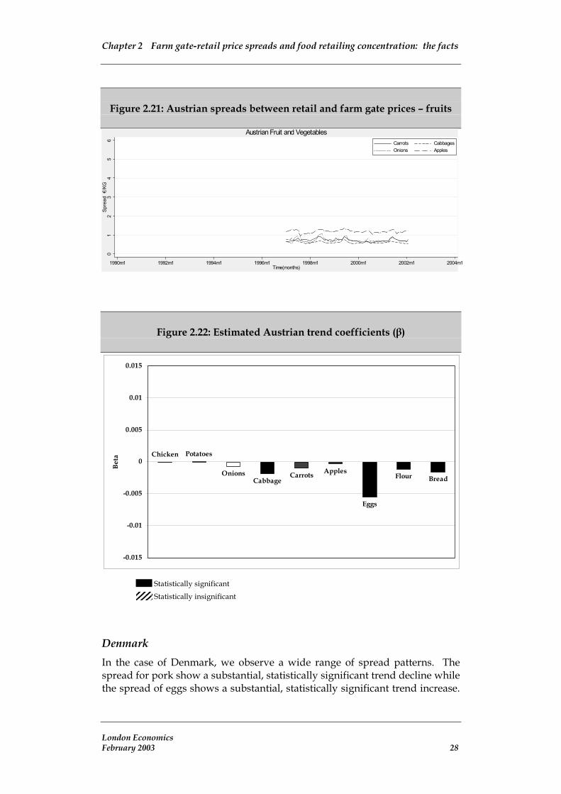
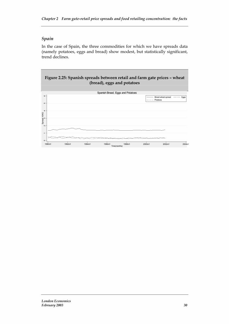
Austria The key fact to note in the case of Austria is that all the commodities show very small or no significant trend declines in their spreads, with the exception of eggs, which posts a more substantial trend decline (Figure 2.20 to Figure 2.22).
Figure 2.20: Austrian spreads between retail and farm gate prices – chicken,
eggs, potatoes, wheat (bread and flour)
01
23
45
6Sp
read
€/K
G
1990m1 1992m1 1994m1 1996m1 1998m1 2000m1 2002m1 2004m1Time(months)
Chicken EggsPotatoes Bread-wheat spreadFlour-wheat
Austrian Chicken, Eggs, Potatoes, Bread and Flour
London Economics February 2003 27
Chapter 2 Farm gate-retail price spreads and food retailing concentration: the facts
Figure 2.21: Austrian spreads between retail and farm gate prices – fruits
and vegetables 0
12
34
56
Spre
ad €
/KG
1990m1 1992m1 1994m1 1996m1 1998m1 2000m1 2002m1 2004mTime(months)
1
Carrots CabbagesOnions Apples
Austrian Fruit and Vegetables
Figure 2.22: Estimated Austrian trend coefficients (β)
Chicken Potatoes
OnionsCabbage
Carrots Apples
Eggs
Flour Bread
-0.015
-0.01
-0.005
0
0.005
0.01
0.015
Beta
Statistically significant Statistically insignificant
Denmark In the case of Denmark, we observe a wide range of spread patterns. The spread for pork show a substantial, statistically significant trend decline while the spread of eggs shows a substantial, statistically significant trend increase.
London Economics February 2003 28

Chapter 2 Farm gate-retail price spreads and food retailing concentration: the facts
Finally, the potatoes and wheat/bread spreads show a modest trend increase while the wheat/flour spread is broadly stable.
Figure 2.23: Danish spreads between retail and farm gate prices – pork,
wheat (bread and flour) eggs and potatoes
01
23
45
67
8Sp
read
€/K
G
1990m1 1992m1 1994m1 1996m1 1998m1 2000m1 2002m1 2004m1Time(months)
Pork Bread-wheat spreadFlour-wheat EggsPotatoes
Danish Pork, Bread, Flour, Eggs and Potatoes
Figure 2.24: Estimated Danish trend coefficients (β)
Pork
Potatoes
Eggs
Flour
Bread
-0.015
-0.01
-0.005
0
0.005
0.01
0.015
Beta
Statistically significant
Statistically insignificant
London Economics February 2003 29
Chapter 2 Farm gate-retail price spreads and food retailing concentration: the facts
Spain In the case of Spain, the three commodities for which we have spreads data (namely potatoes, eggs and bread) show modest, but statistically significant, trend declines.
Figure 2.25: Spanish spreads between retail and farm gate prices – wheat
(bread), eggs and potatoes
01
23
45
6Sp
read
€/K
G
1990m1 1992m1 1994m1 1996m1 1998m1 2000m1 2002m1 2004m1Time(months)
Bread-wheat spread EggsPotatoes
Spanish Bread, Eggs and Potatoes
London Economics February 2003 30

Chapter 2 Farm gate-retail price spreads and food retailing concentration: the facts
Figure 2.26: Estimated Spanish trend coefficients (β)
PotatoesEggs Bread
-0.015
-0.01
-0.005
0
Beta
Statistically significant
Statistically insignificant
Italy In the case of Italy, most spreads exhibit very small upward trends (eggs, flour and bread) while the trend coefficient of the chicken spread is not statistically significant.
London Economics February 2003 31

Chapter 2 Farm gate-retail price spreads and food retailing concentration: the facts
Figure 2.27: Italian spreads between retail and farm gate prices – chicken,
wheat (bread and flour), eggs 0
12
34
56
Spre
ad €
/KG
1990m1 1992m1 1994m1 1996m1 1998m1 2000m1 2002m1 2004mTime(months)
1
Bread-wheat spread Flour-wheat spreadEggs Chicken
Italian Chicken, Bread, Flour and Eggs
Figure 2.28: Estimated Italian trend coefficients (β)
Chicken
EggsFlour
Bread
-0.015
-0.01
-0.005
0
0.005
0.01
0.015
Beta
Statistically significant Statistically insignificant
Summary of the trend analysis of the spreads Below in Table 2.3 we present a summary overview of the analysis of trend changes in the farm gate-retail price spreads.
London Economics February 2003 32

Chapter 2 Farm gate-retail price spreads and food retailing concentration: the facts
While many different trend patterns were observed, a number of facts are worth highlighting:
1. The beef spread is the only spread showing a large trend increase in many countries. This is indeed the case in 4 out the 5 countries for which we have data. These are the United Kingdom, France, Germany and Netherlands.
2. In the case of lamb, quite different trends are observed with trend increases in the United Kingdom and Ireland and trend declines in France and Germany.
3. A similar wide range of trend patterns is observed in the case of pork and eggs.
4. The chicken and various fruit and vegetable spreads show either no significant trend or very small trend decreases.
5. Finally, the trend changes in the wheat/bread and wheat/flour spreads range from very small positive to small negative.
London Economics February 2003 33

Chapter 2 Farm gate-retail price spreads and food retailing concentration: the facts
Table 2.3: Summary overview of trends in farm gate-retail price spreads
Trend coefficient UK France Germany Ireland Nether. Austria Denmark Spain Italy
Large positive
Lamb* Eggs Beef Potatoes
Beef Beef Beef Eggs
Small positive
Pork Tomatoes Lamb Potatoes Potatoes Bread
Eggs
Very small positive
Eggs Bread Pork
Bread Eggs Beef
Bread Flour
Not statistically significant
Tomatoes Apples Flour
Potatoes Pork
Onions Tomatoes Carrots Bread
Chicken Onions Carrots Apples
Chicken
Very small negative
Cabbage Carrots Onions Bread
Chicken Pears Apples Cabbage Carrots Onions Eggs Chicken
Pork Bread Eggs
Chicken Potatoes
Flour Potatoes
Small negative
Lamb Bread Flour Cabbage
Bread Eggs
Large negative
Lamb Eggs Pork
2.2 Concentration in the European food retail industry
2.2.1 Changes in the structure of food retailing in the nineties
In the past ten years, Europe has witnessed a sharp increase in the trend of mergers and acquisitions within the retail sector and the food retail sector in particular. This increase in concentration has attracted attention within both the academic world and amongst antitrust practitioners. As a result, a wave of theoretical work on the economics of the retail sector, with an eye to antitrust implications, has recently been emerging.
London Economics February 2003 34

Chapter 2 Farm gate-retail price spreads and food retailing concentration: the facts
One of the key features of the food retail sector in the nineties is a clear trend towards larger size food retail outlets across all EU Member States (see Annex 4 for details).
While smaller shops still make up the bulk of food retail outlets in Europe, they accounted for only 21% of total food retail turnover in 2000 (Table 2.4).
Table 2.4: European food retail outlets, numbers and turnover, 2000
Numbers Share of total
turnover
Hypermarkets (>2,500 m2) 5,293 31
Large supermarkets (1,200 - 2,500 m2) 14,805 22
Small supermarkets (400 – 1,200 m2) 39,559 23
Superettes + traditionals (<400 m2) 341,094 21
Other 5,260 2
Total 407,740 100
Source: ACNielsen (2003).
As Figure 2.29 overleaf illustrates, the lowest size category dominates in all countries except in Norway, where the “small supermarkets” category is the largest in terms of number of stores. Traditional shop types clearly outnumber larger food stores, and in particular the hypermarkets.
Nevertheless, the larger store types dominate the total turnover in the European food retailing sector (Figure 2.30). These modern distribution formats, particularly supermarkets, hypermarkets and discount stores have developed vigorously in the past two decades, chiefly at the expense of traditional stores (Eurostat, 1996).
London Economics February 2003 35

Chapter 2 Farm gate-retail price spreads and food retailing concentration: the facts
Figure 2.29: European food retailing industry: types of shops as a % of total
number of shops.
0.0%
20.0%
40.0%
60.0%
80.0%
100.0%
Austria Belgium Denmark
Finland France
Germany Great Britain
GreeceIrealnd
ItalyNetherlands
NorwayPortugal
Spain Sweden
Switzerland EUROPE
hypermarkets (>2,500 m2) large supermarkets (1,200 - 2,500 m2) small supermarkets (400 - 1,200 m2) other
Source: AC Nielsen (2003).
superettes + traditionals (<400 m2) other
superettes + traditionals (<400 m2) other
Figure 2.30: European food retailing industry: market share of various types
of stores as a % of total turnover.
0 10 20 30 40 50 60
Austria Belgium
Denmark Finland
France Germany
Great BritainGreece
Irealnd
ItalyNetherlands
NorwayPortugal
SpainSweden
Switzerland EUROPE
hypermarkets (>2,500 m2) large supermarkets (1,200 - 2,500 m2) small supermarkets (400 - 1,200 m2) Source: Eurostat (1996).
A more recent type of shop, the discount store, has a very high presence in Germany (where it was pioneered), Austria, and Belgium (see Annex 4 for
London Economics February 2003 36

Chapter 2 Farm gate-retail price spreads and food retailing concentration: the facts
details). The discount store also seems to be gaining ground in the Netherlands and Portugal. This type of shop has low market penetration in most other European countries.
Finally, associative retail formats such as buying organisations and co-ops, have a very strong presence in Italy, Finland and Switzerland, mainly in the form of voluntary chains. Spain also shows a high penetration of that form of retailing.
2.2.2 Concentration in European food retailing The trend towards larger food retail outlets resulted in a sharp increase in the concentration of the food retailing industry in a number of EU Member States.
It is important to note that there exist no consistent data sources of concentration within the food retail industry and, in our work, we have used information available from Mintel, M+M Planet Retail and Dobson (2002).
Below, in Table 2.5, we present summary measures of concentration across the major European countries based on the Mintel data. The first four columns show different concentration ratios and Ci is the sum of the market shares of the top i firms. For example, C1 is the market share of the top firm and C5 is the market share of the top five firms.
We also provide estimates of the Herfindhal index (HI), another frequently used indicator of concentration in competition analysis. This index is simply the sum of the squares of the market shares of all the firms. The index takes a value of 1 in a pure monopoly situation and approaches 0 when the market is characterised by perfect competition.
One should note that the measures reported in Table 2.5 are approximations of the true degree of concentration as sales information for some retailers is missing in the case of a few countries. We estimate that the Mintel data are missing market share information for about 5% of the market in Austria, Ireland and the United Kingdom, for about 10% in Belgium and Portugal, and for about 15% in France.
London Economics February 2003 37

Chapter 2 Farm gate-retail price spreads and food retailing concentration: the facts
Table 2.5: European food retail concentration measures (2001-2002)
C1 C3 C4 C5 HI
Austria 31.0% 73.6% 82.9% 87.4% 0.21
Belgium 25.3% 63.2% 72.3% 80.7% 0.16
France 21.6% 47.6% 57.2% 66.2% 0.11
Germany 26.3% 58.0% 69.1% 77.7% 0.15
Ireland 31.6% 67.5% 80.5% 89.9% 0.20
Italy 19.4% 52.9% 64.9% 72.7% 0.12
Netherlands 40.8% 70.7% 76.1% 80.1% 0.23
Portugal 26.0% 56.4% 67.1% 76.7% 0.15
Spain 30.9% 56.3% 65.9% 74.0% 0.15
United Kingdom 23.8% 53.0% 62.9% 68.4% 0.12
Average 27.7% 59.9% 69.9% 77.4% 0.16
Difference* 21.4% 26.0% 25.7% 23.7% 0.09
Source: Mintel (2002). Note: * Difference between highest and lowest.
The Mintel data suggests that the Austrian, Dutch and Irish markets are the European food retail markets with the highest levels of concentration among the EU Member States for which Mintel provides data.
The Netherlands has the highest single-firm concentration ratio (C1), 40.8% and the highest HI, 0.23. Ireland and Austria show C1 of just above 30% and a HI of 0.20 or a shade above.
These three countries also post the highest three-firm concentration ratios and, together with Belgium, the highest four-firm (C4) and five–firm (C5) concentration ratios.
Of particular interest is the fact the variation in concentration ratios8 across EU Member States is lower at the five-firm level than at the three-firm level, suggesting that, within the top five firms the competition dynamics may differ significantly across European countries.
A second important point to note is that the United Kingdom’s food retailing concentration is below EU average, and below that observed in important food markets such as Germany, Italy (only for C4 and C5) and Spain, but slightly above the French figures.
8 As measured by the difference between the highest and lowest concentration ratios.
London Economics February 2003 38

Chapter 2 Farm gate-retail price spreads and food retailing concentration: the facts
In terms of dominance of the food retailing industry, we note that both Spain’s and the Netherlands’ largest food retail groups have the largest market share advantage over their two closest competitors. The Dutch market leader has 40.8% market share and the two closest rivals achieve a combined market share of only 30%. The Spanish leader, with a 30.9% market share, has a higher market share than the combined market shares of the second and third largest retailers of only 25.4%. The Netherlands and Spain are the only two countries in the sample where we observe such a large difference between the market share of the top food retailer and that of its most immediate competitors.
Table 2.6 provides information on how concentration in the food retail sector has evolved through the nineties in Europe. These data are not directly comparable with those in the previous table as they come from a different source. Nevertheless, they provide useful information on the general trends in food retailing concentration.
Of particular interest is the fact that, while food-retailing concentration has increased markedly in the vast majority of EU Member States over the period 1993-2002, the United Kingdom posts a much more subdued increase. The major food markets (France, Germany, Italy, Spain) in continental Europe post increases in the five-firm level concentration ratio in the range of 20 to 40 percentage points while the same concentration ratio grew by only 7.7 percentage points in the United Kingdom over the same period.
London Economics February 2003 39
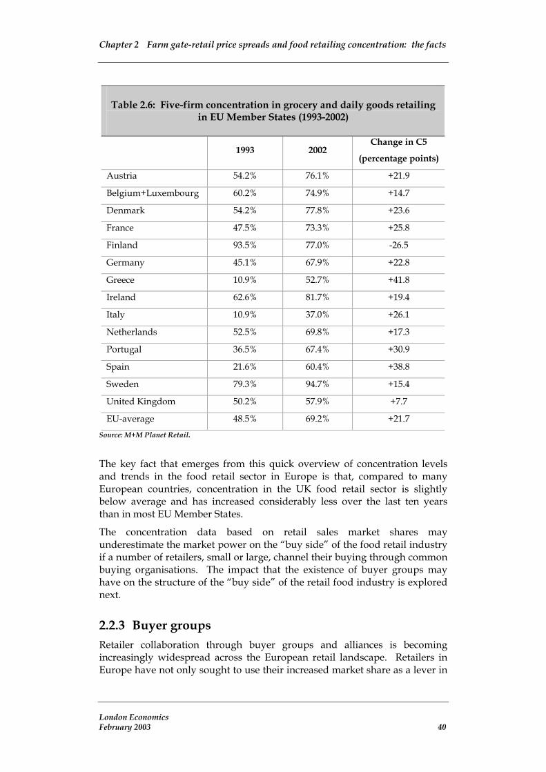
Chapter 2 Farm gate-retail price spreads and food retailing concentration: the facts
Table 2.6: Five-firm concentration in grocery and daily goods retailing in EU Member States (1993-2002)
1993 2002
Change in C5
(percentage points)
Austria 54.2% 76.1% +21.9
Belgium+Luxembourg 60.2% 74.9% +14.7
Denmark 54.2% 77.8% +23.6
France 47.5% 73.3% +25.8
Finland 93.5% 77.0% -26.5
Germany 45.1% 67.9% +22.8
Greece 10.9% 52.7% +41.8
Ireland 62.6% 81.7% +19.4
Italy 10.9% 37.0% +26.1
Netherlands 52.5% 69.8% +17.3
Portugal 36.5% 67.4% +30.9
Spain 21.6% 60.4% +38.8
Sweden 79.3% 94.7% +15.4
United Kingdom 50.2% 57.9% +7.7
EU-average 48.5% 69.2% +21.7
Source: M+M Planet Retail.
The key fact that emerges from this quick overview of concentration levels and trends in the food retail sector in Europe is that, compared to many European countries, concentration in the UK food retail sector is slightly below average and has increased considerably less over the last ten years than in most EU Member States.
The concentration data based on retail sales market shares may underestimate the market power on the “buy side” of the food retail industry if a number of retailers, small or large, channel their buying through common buying organisations. The impact that the existence of buyer groups may have on the structure of the “buy side” of the retail food industry is explored next.
2.2.3 Buyer groups Retailer collaboration through buyer groups and alliances is becoming increasingly widespread across the European retail landscape. Retailers in Europe have not only sought to use their increased market share as a lever in
London Economics February 2003 40

Chapter 2 Farm gate-retail price spreads and food retailing concentration: the facts
negotiating with suppliers but have increasingly sought to collaborate with other retailers to further enhance their bargaining power.
There exists two main types of buyer groups: those that bring together many small retailers and thus work to counterbalance the increasing market power of the large supermarkets; and those that bring together two or more of the large retailers, giving them even stronger market power.
The buying groups representing the smaller retailers are actually the largest buying groups in some countries.
In terms of assessing buyer power, what is most important is the concentration in terms of buying groups rather than the concentration in terms of food retailer sales. A retail market characterised by a large number of small retailers (low concentration on the sell side) may nonetheless be a market where retailers have high buying power if they are organised into large buying groups. Indeed, in some countries, the “buy side” of the food retail sector exhibits much higher concentration indicators than the “sell side”.
Below, we provide an index of concentration in food retail where market concentration is “corrected” to take account of market concentration at the buying level.
London Economics February 2003 41

Chapter 2 Farm gate-retail price spreads and food retailing concentration: the facts
Table 2.7: Five-firm concentration ratios adjusted for buying groups, 1999
Excluding Buying Groups
Including Buying Groups
Buying groups in top 5
Austria 60.2 58.6
Belgium+Luxembourg 60.9 66.0 BLOC
Denmark 56.4 76.6 Supervib
Finland 68.4 70.5 Tradeka/Elanto
France 56.3 64.7 LUCIE, ITM, Opera
Germany 44.1 52.5 Markant
Greece 26.8 33.5 Elomas, Elonki, ORA
Ireland 58.3 58.3
Italy 17.6 26.4 ICMS, Italia Distribuzione, Intermedia, Mecades
Netherlands 56.2 71.7 SuperUnie, TSN
Portugal 63.2 67.0 Uniarme
Spain 40.3 63.7 Euromadi, IFA
Sweden 78.2 80.6 Axfood Sviege
UK 56.2 56.2
EU-15 (weighted average) 48.9 60.5 Source: Dobson (2002) and LE calculations.
As we can see from above, the average EU-15 retail concentration is much higher when we take into account the buyer power of the top retailers. The impact of buyer group concentration is especially important in Denmark, France, Germany, Greece, Italy, the Netherlands and Spain. In the United Kingdom, the inclusion of buyer groups does not change the picture emerging from the “sell” side of the food retail industry.
In the next section, we will explore whether the concentration levels and trends highlighted in this section have had any impact on observed farm gate-retail price spreads in the United Kingdom and a number of other EU Member States.9
9 The advent of the Single Market in the EU and the rapid growth of pan-European, or world, food retail chains raises the issue of whether it is still appropriate to consider the national market as the relevant geographical market for an analysis of buying power. A number of experts that we consulted suggested that, at the present time, food products are still typically bought nationally. Thus, for the purpose of the present analysis, we will use the national market as the relevant geographical market.
London Economics February 2003 42

Chapter 2 Farm gate-retail price spreads and food retailing concentration: the facts
2.3 Simple correlation analysis between farm gate-retail price spreads and concentration in the retail food sector
2.3.1 Introduction In this section we report some preliminary analysis of the relationship between concentration in the European food retailing industry and the farm gate-retail price spreads of the commodities described earlier.
This correlation analysis is undertaken for the following four groups of spreads:
1. Cereals (wheat/flour and wheat/bread);
2. Red meat (beef, lamb and pork);
3. Poultry and eggs;
4. Fresh fruit and vegetables
We use two different measures of the farm gate-retail price spread in our correlation analysis. The first is simply the difference between retail price and the farm gate price expressed in € across all countries (absolute spread) and the second measure is the absolute spread expressed as percentage of the farm gate price (relative spread).
The concentration ratio used in the analysis is the C5 ratio, i.e. the market share of the top five food retailers in the domestic market.
2.3.2 Correlation between spreads and concentration levels in 2000-2001
The correlation results reported in Table 2.8 show that, over the period 2000-2001, the correlation between the level of spreads (in absolute terms or relative terms) and the level of the C5 concentration ratio is low.
The highest correlation coefficient is obtained in the case of cereals of around 0.3, using the absolute and relative spreads estimates.
London Economics February 2003 43

Chapter 2 Farm gate-retail price spreads and food retailing concentration: the facts
Table 2.8: Correlation between the farm-retail spread and the C5 concentration ratio (2000-2001)
Correlation Coefficient
Agricultural Product Group Absolute Spread Relative Spread Ratio
Cereals 0.31 0.38
Red Meat 0.14 0.03
Poultry and Eggs 0.24 0.12
Fresh fruit and vegetables 0.15 0.07
2.3.3 Correlation between changes in spreads and concentration levels 1993/94 to 2000/01
Even more interesting are the results of the correlation analysis of changes in the levels of farm gate-retail spreads and changes in the level of concentration in the European food retailing industry.
In Table 2.9 below, we report the correlation between the change in the level of the various spreads and the change in the level of the C5 concentration ratio. The change in these two variables is calculated as the difference between the average level prevailing in 1993 and 1994 and the average level prevailing in 2000 and 2001.10
In the case of red meats, poultry and eggs, and fresh fruits and vegetables, the correlation between changes in the spreads and the concentration level in food retailing industry is actually negative.
Table 2.9: Correlation between changes in the spreads and the C5 concentration ratio (1993/1994 to 2000/2001)
Correlation Coefficient
Agricultural Product Group Absolute Spread Relative Spread Ratio
Cereals 0.23 0.35
Red Meat -0.46 -0.28
Poultry and Eggs -0.61 -0.71
10 We did not extend the analysis to 2002 because the 2002 information for many spreads was still incomplete when the analysis was undertaken in 2003.
London Economics February 2003 44

Chapter 2 Farm gate-retail price spreads and food retailing concentration: the facts
Table 2.9: Correlation between changes in the spreads and the C5 concentration ratio (1993/1994 to 2000/2001)
Correlation Coefficient
Agricultural Product Group Absolute Spread Relative Spread Ratio
Fresh fruit and vegetables -0.46 -0.23
We have repeated the analysis for two different subsamples to assess the robustness of the results when breaking the sample in two. In Table 2.10 and Table 2.11 we present the correlation between changes in the spreads and C5 concentration ratio for the periods 1993/1994 to 1996/1997 and for 1996/1997 to 2000/2001. Two points are worth noting. The first one is that the results change noticeably relative to those reported in Table 2.9. This means that the correlation is not constant over the period 1993 to 2001. The second one is that in none of the two sub-periods a correlation coefficient is greater than 0.4, and most of the correlation coefficients are negative.
Table 2.10: Correlation between changes in the spreads and the C5 concentration ratio (1993/1994 to 1996/1997)
Correlation Coefficient
Agricultural Product Group Absolute Spread Relative Spread Ratio
Cereals -0.10 0.04
Red Meat 0.35 0.31
Poultry and Eggs 0.08 0.05
Fresh fruit and vegetables 0.39 0.26
London Economics February 2003 45

Chapter 2 Farm gate-retail price spreads and food retailing concentration: the facts
Table 2.11: Correlation between changes in the spreads and the C5 concentration ratio (1996/1997 to 2000/2001)
Correlation Coefficient
Agricultural Product Group Absolute Spread Relative Spread Ratio
Cereals -0.13 0.11
Red Meat -0.47 -0.03
Poultry and Eggs -0.52 -0.48
Fresh fruit and vegetables -0.37 0.12
Thus, at first glance, it would not appear that increases in the concentration of the European food retailing industry were accompanied by increases in the margins between farm gate prices and food retail prices.
This does not mean that buyer power has not been exercised. As we explain in the next chapter, the exercise of buying power may not necessarily be reflected in a lower price spread if the price reductions obtained on the buyside are passed on by retailers to customers. In such a case, the farm gate-retail price margin may not fall necessarily although the farm gate price will be lower.
Moreover, food retailer concentration is only one of many factors that may affect the size of the spread between farm gate and retail prices. It is possible, however, that a number of other factors affected farm gate-retail price spreads in the nineties and, thus, contribute to obscure the true underlying link between spreads and concentration in the simple two-variable framework of the correlation analysis11.
This is why, later in Chapter 6, we undertake a more in-depth statistical analysis of the behaviour of farm gate-retail price spreads in the nineties, including the effects of a number of potential variables affecting price spreads.
11 A number of other factors may affect the farm gate-retail price margins independently of buying power (foreign market developments, supply and demand shocks, policy changes, etc.
London Economics February 2003 46

Chapter 3 Buying power and farm-retail price spreads
3 Buying power and farm-retail price spreads
3.1 Overview There is no consensus at the present time on the economic and legal meaning of buyer power, although a number of alternative definitions have been put forward. As a result, there has been no clear agreement on the appropriate measurement of buyer power.
The UK Competition Commission, the OECD and the European Commission, all seem to share the view, however, that relatively low market shares in the relevant market may be sufficient to cause effects that are detrimental to competition.
One example of the importance given to buyer power concerns is the European Commission’s assessment of the merger of Carrefour and Promodes. With a combined share of around 30% of food retail distribution in France, the merger did not raise issues of either single firm dominance, or of collective dominance on the sell side of the market. The Commission argued, however, that the buyer power created by the merger, could distort competition. It identified two related mechanisms: the “spiral effect” and the “threat point”. The first refers to the self re-enforcing effect of market share and volume discounts, while the second refers to the power that a buyer of even a small percentage of a producer’s total output can have in affecting its viability as a business.
On the other hand, buyer power can have a positive impact in a situation where intermediate suppliers have substantial market power.
For example, in the food retail sector, an increase in buying power of retailers may countervail (a term coined by Galbraith in 1952) the market power of food manufacturers. Such a situation would particularly benefit consumers if retailers behave competitively in selling, i.e. if there is a low degree of selling power in the retail sector, which would guarantee that the buying price reductions that retailers obtain would be passed on to final consumers.
3.2 Buyer power: definition “Buyer power” can be simply defined as the market power that retailers, or buyers in general, possess vis-à-vis their suppliers. The presence of buyer power at some point in the supply chain is now a market feature that is taken into consideration whenever a careful analysis of the sector is required.
In their report on buyer power in 1981, the Committee of Experts on Restrictive Business Practices defined buyer power as “a situation which exists when a firm or a group of firms, either because it has a dominant
London Economics February 2003 47

Chapter 3 Buying power and farm-retail price spreads
position as a purchaser of a product or service or because it has strategic or leverage advantages as a result of its size or other characteristics, is able to obtain from a supplier more favourable terms than those available to other buyers” (OECD, 1981).
From the point of view of theoretical research, a relatively large amount of attention has been devoted to the assessment of the effects that buyer power might have on the functioning of manufacturing or retail industries and the welfare implications of such buying power.
Comparatively little attention, on the other hand, has been devoted to analysing the origin of buyer power. In other words, little theoretical or empirical research has focused on what factors confer to a firm buyer power or more buyer power than to its competitors.
One reason for the relative absence of theoretical work on the causes of buyer power is the loosely held view that buyer size determines buyer power. This view, though being intuitively appealing, does not correspond to the actual functioning of modern retail purchase markets because it does not take into account the way in which retailers actually compete.
3.2.1 Buyer power: scope measure The existence of high buyer concentration need not, in itself, imply that significant buyer power is being exercised. An important factor is the structure of the selling side of the market, particularly whether or not a seller can easily divert sales from a particular buyer to other buyers.
The proportion of food going to the processing industry has changed in recent years and may have had some impact in the bargaining relationships along the supply chain.
Blair and Harrison (1992) argue that buyer power measures should take into account the elasticity of supply. The intuition underlying this point is that, if the supply of a good is perfectly elastic, even a pure monopsonist (i.e., a sole buyer) cannot exert buying power.
The less elastic the supply is the greater is the potential for exercising buy power. For example, food products which are perishable and have no alternative outlets (i.e. whose supply is inelastic) are much likely to be subjected to buyer power than products that are storable and/or are brought to market through a wide range of channels (i.e. whose supply is likely to be much more elastic).
However, as noted by Jacobson and Dorman (1992), elasticities of supply are difficult to measure in practice, and hence, despite its theoretical appeal, this supply-elasticity concept is less likely to be practical than measures based on market share information.
London Economics February 2003 48

Chapter 3 Buying power and farm-retail price spreads
3.3 Retailer buyer power and farm gate-retail price spreads
The empirical relationship between buyer power and the level of farm gate-retail price spreads is often complex.
In general, we cannot assume that high levels of buyer power will necessarily lead to high farm gate-retail price spreads, or even high profit margins.
For example, it is possible that, even though retailers have a large amount of buyer power and are therefore able to extract lower prices from farmers and food producers in general, at the same time, they compete with each other very aggressively in the sell side of the market. Any supply price reductions achieved through the exercise of buying power may be fed straight into retail prices.
Moreover, other factors will affect the size of the spread between farm gate and retail prices. For example, increases in the costs of inputs used by any intermediary in the supply chain or by the retailer will directly impact on the spread. Structural changes such as a) the growth or decline of co-operative sellers, intermediaries and buyers, b) changing consumer tastes and food consumption habits, c) changes in the end use of the agriculture product (food processing versus direct retail sales), d) the emergence of new competitors to the agricultural product (organic products, foreign imports, etc), e) foreign market developments, f) supply and demand shocks may all impact on either the retail or farm gate price and disturb the long-run relationship that may exist between these two price variables.
Essentially, one can distinguish three broad types of methodological approaches to the empirical analysis of farm gate-retail price spreads. The first, and oldest, is based on the structure-conduct-performance paradigm and relates performance indicators such as profitability to the structure of an industry.
The second approach, based on the New Empirical Industrial Organisation, attempts to model the behaviour of firms within an industry to determine whether it is characterised by market power. The implementation of this approach is very complex and requires the researcher to make a number of assumptions which, if not true, can undermine the robustness of the results obtained in the empirical analysis.
Finally, a third approach examines the time series properties of the farm end retail prices. This astructural approach essentially aims to uncover the relationship between the farm gate price and the retail price that is present in the data.
In our empirical work, we will rely on the astructural time series analysis approach and on the reduced form approach.
London Economics February 2003 49

Chapter 4 Asymmetric price transmission: review of the literature
4 Asymmetric price transmission: review of the literature
4.1 Introduction The relationship between farm and retail prices has been the subject of numerous research studies that aim to understand why marketing margins for agricultural products have changed over time.
It may seem quite natural to assume that retail prices depend on the price charged at the farm gate. After all, the retail price should include the farm price plus wholesale and retail costs, plus any margins earned at each level. However, if we think about changes in the price, the direction of causality may be reversed.
For example, a demand shock that starts with the consumers buying less hits the retailers first, forcing them to lower their own prices. Retailers might be able to pass this on back along the chain. In this case, a change in the retail price would help to explain why there has been a change in the farm gate price and not vice versa.
In some cases, pricing power of few firms may imply that retail prices respond more quickly to a cost increase than to a decrease. Hence, increases in input prices, which reduce marketing margins, are transmitted faster and more completely than decreases as a result of market power. If this is the case, the price transmission is said to be asymmetric along the marketing chain.
However, it is important to note that asymmetric transmission can occur for a number of other reasons, and one cannot conclusively conclude that market power or buying power exists because one observes asymmetric price transmission.
The object of price transmission analysis is to provide answers to the following questions: by how much is a change in the farm price reflected in the retail price and vice versa? Is there a difference in the way that the retail price adjusts to an increase or a decrease in farm price and vice versa?
Many models of price transmission assume a long-run relationship between the price series after transient effects (such as exogenous elements affecting production or consumption) have disappeared. Thus, the two variables may drift apart in the short run due to a change in policy or seasonal factors, but if they continue to be too far apart in the long run, then economic forces, will bring them together. Asymmetric transmission is investigated by testing statistically whether changes (increases and decreases) in the prices at one end of the marketing chain affect (or are transmitted to) the other end.
In this chapter we start by reviewing the main causes of asymmetric price transmission that have been reported in the literature. Then, we review the
London Economics February 2003 50

Chapter 4 Asymmetric price transmission: review of the literature
literature that has studied asymmetries in farm price transmission for agricultural commodities. The main findings are summarized at the end of the chapter.
4.2 Causes of asymmetric price transmission Imperfect price transmission might exist when price changes at one end of the supply chain are not immediately reflected at the other end. Imperfect price transmission can be of three different types.
In the first place, price changes may not be fully transmitted along the marketing chain. Thus, prices at the upstream and downstream ends of the food chain would be independent of each other. This would imply that prices are insulated from any developments or shocks occurring at the other end of the chain. In practice, it is rare to observe full independence of prices at each end. However, sometimes it has been reported that the direction of the transmission goes in one direction only, e.g. from farm gate to retail, with no evidence of transmission from retail to farm gate.
The second type of imperfect transmission is a transmission with some time lag. In this case, increases or decreases in one end of the chain are not transmitted instantaneously but instead distributed over time. For example, an increase in the price at the farm gate takes a number of periods to be fully transmitted to the retail price.
Finally, there could be imperfect transmission in the form of asymmetric reaction to positive and negative shocks. The term “asymmetry” signifies that the reaction of the price at one level of the marketing chain to a price change at another level depends on whether the initial change is positive or negative.
The literature identifies market structure and the presence of non-competitive behaviour as the main cause for asymmetry in farm-retail price transmission.
However, some authors note that imperfect price transmission may be due to other factors, such as adjustment costs. For example, costs related to labelling, advertising or goodwill make remarking of prices expensive and give rise to price reactions with some time lags. Other causes of asymmetric price response that have been reported are factors such as political intervention or inventory management. We will describe each of these causes in a different subsection below.
Market power Economic theory suggests that profit-maximizing firms in competitive markets should adjust their prices quickly and symmetrically to input cost decreases or increases. However, farmers at the beginning of the chain and consumers at the other end often believe that less than perfect competition in the intermediate stages of the processing allows middlemen to obtain
London Economics February 2003 51

Chapter 4 Asymmetric price transmission: review of the literature
“excess” profits (see Meyer and von Cramon-Taubadel, 2002, for a complete survey).
The argument for asymmetries in price transmission rests on the fact that supply chains for food products are often much less concentrated at the farm level than higher up. This could cause oligopolistic processors and retailers to react collusively and transmit more rapidly shocks that squeeze their margin than shocks that stretch it (von Cramon-Taubadel, 1998).
Market power will thus lead to positive asymmetry in an oligopolistic retail environment: cost increases will produce an immediate increase in output prices as retail margins are squeezed, whereas cost decreases will not be instantaneously transmitted to price decreases because firms will maintain prices above the competitive level (Borestein et al., 1997).
Other authors do not specify whether market concentration will lead to positive or negative asymmetry. Bailey and Brorsen (1989) use the notion of a kinked demand curve to explain asymmetries. They argue that if a firm conjectures that competitors will match an increase in output prices, but not an equivalent reduction, positive asymmetry transmission will result. Otherwise, if a firm believes that no competitor will match a price increase but all will match a price cut, negative asymmetry will result. Concentration is perhaps a necessary but not a sufficient condition for the exercise of market power. The underlying conjecture may be based on “learning by doing” and need not reflect collusion.
There are other explanations of imperfect transmission in the context of oligopolistic and oligopsonistic markets. The risk of provoking a price war may make firms reluctant to lower prices, and price adjustment might take place only after some lags. In oligopolistic markets with unspoken collusion, firms will use price changes to signal the unspoken agreement (Balke et al., 1998 and Brown and Yucel, 2000). When input prices rise, each firm will quickly adjust prices upwards to signal that collusion will be maintained, whereas they will wait to lower output prices to avoid undermining a tacit agreement.
Different levels of profitability can lead to asymmetry according to Bedrossian and Moschos (1998). If a firm is relatively profitable, then it can take greater risks in delaying a price adjustment following a fall in input prices.
Finally, Ward (1982) has reported perishability of goods as an important source of asymmetric transmission. In this context, retailers could avoid raising prices for fear of being left with a spoiled product.
Adjustment costs Adjustment costs provide an alternative explanation for asymmetric price transmission. The costs of labelling, advertising or promoting goodwill make remarking of prices expensive. Thus, the reaction to a given rise in price might take place with lags or might be transmitted with some delay.
London Economics February 2003 52

Chapter 4 Asymmetric price transmission: review of the literature
Some authors (Ball and Mankiw, 1994; Zachariasse and Bunte, 2003) have stressed the importance of the menu costs of remarking prices (such as the cost of reprinting catalogues).
The model of Ball and Mankiw (1994) uses inflation as an explanation for asymmetric price transmission. In this case, firms would increase prices to correct for accumulated and anticipated inflation. However, transmission of negative shocks would be less necessary as inflation would already have adjusted the prices.
Other causes There have been additional explanations for the existence of price transmission.
Kinnucan and Forker (1987) explain how government intervention can lead to asymmetric intervention. Processors and retailers may believe that a reduction in price may be temporary because it will trigger government intervention through support prices. In this context, processors and retailers will not react to a reduction in farm prices but they will quickly respond to increases in farm prices because they will believe it is more likely to be permanent.
Accountancy rules and inventory valuation may also be a reason for transmission sluggishness. For example, a firm which measures inventories by historical costs (FIFO or first-in-first-out) may not change output prices to cost changes immediately until the stock of inventories bought at old prices is depleted. Balke et al. (1998) show that the FIFO accounting method can cause asymmetries in the price transmission. On the contrary, when a firm values inventories through replacement cost criterion (LIFO or last-in-first-out), the firm's output prices will react much quicker to a cost change.
4.3 Empirical findings Numerous studies have examined asymmetric price transmission in agricultural markets. Such studies have examined different products, geographic areas and time periods.
The bulk of the literature has studied transmission in the sectors of fresh vegetables and meats. Below, we devote two separate subsections to describe the main studies in the fresh vegetables and meat markets, focusing mainly on studies examining the European farm gate-retail price spreads.
4.3.1 Fresh vegetables Previous studies on price transmission have found different conclusions for the sector of fresh vegetables.
The study by Hassan and Simioni (2001) tests the existence of asymmetry between shipping-point and retail prices for French tomato and chicory. The
London Economics February 2003 53

Chapter 4 Asymmetric price transmission: review of the literature
authors use weekly data prices from the French Ministry of Agriculture, collected at different stages of the marketing channel (shipping, wholesaling and retailing) and according to product variety and area of production.
The study analyses forty-two pairs of shipping-point and retail prices (twenty-two for tomato and twenty for chicory), which have been proposed according to different product categories and regions. The results show that for each pair of shipping-point and retail prices there exists a long-run equilibrium relationship. Moreover, the dynamics of the models suggest directional causation from shipping-point price to retail price for the considered products. However, the short-run adjustment mechanisms seem to be different for the two categories of products. In the tomato case, half of the short-run models are shown to be symmetric. In the cases where asymmetry prevails, the estimates suggest that reductions in shipping-point prices appear to be passed on to the retail prices faster than increases in the shipping-point price. In the chicory case, the short-run adjustment mechanisms are also more often symmetric than asymmetric. In the cases where asymmetry prevails, it seems that increases in shipping-point prices seem to be passed on to the retail prices faster than declines in the shipping-point price.
According to Hassan and Simioni, these findings do not give evidence to the widespread assertion that middlemen with speculative aims systematically use price changes occurring in the first stages of a marketing channel. Overall, in only seven relationships out of forty-two (and mainly for chicory) it is found that shipping-point price increases are completely and rapidly passed on to consumers, while there is a slower and less complete transmission of shipping-point price declines. In eleven cases (mainly for tomatoes) the converse result holds. But in the majority of cases price transmission appears to be symmetric.
In another study Zachariasse and Bunte (2003) examine price transmission for potato products in the Netherlands and find asymmetric transmission. The authors find that retailers follow negative price shocks at the farm level, but not positive price shocks. In this case farmers benefit from the asymmetry.
Other studies of price transmission in the sector of fresh vegetables also reach different conclusions. For example, Worth (2000) examines the price transmission of six vegetables between free-on-board shipping-point prices and retail prices. Using monthly data from the National Agricultural Statistics Service at the US, he finds no evidence of price asymmetry for celery, lettuce, onions and potatoes; whereas for carrots and tomatoes there seems to be some evidence that retail prices show a greater response to shipping-point price increases.
On the other hand, Ward (1982), using US data for various fresh vegetables in different cities, reports some evidence of asymmetric transmission in the direction of wholesale to retail: price decreases at the wholesale are transmitted more often to the retail level than are wholesale price increases.
London Economics February 2003 54

Chapter 4 Asymmetric price transmission: review of the literature
The study by Barallat, McLaughlin, and Lee (1987) compares the performance of alternative models of marketing margin behaviour with application to the Spanish fresh potato market. The research uses six alternative models to estimate and forecast marketing margins but it does not provide any explanation of the evolution of the potato margins in Spain.
4.3.2 Meat products An extensive literature has examined price linkages among farm, wholesale, and retail markets for meat and livestock products.
In a recent study, Tiffin and Dawson (2000) examine the farm-retail price spread for lamb using monthly UK data for 1979-1993. The data are from the Meat and Livestock Commission and relate to England and Wales from January 1979 to December 1993. Nominal producer prices for lamb are dead-weight equivalent livestock prices (p/lb); nominal retail prices are average lamb prices. Real prices are calculated using the RPI.
The results of the study show that a long-run relationship exists between producer and retail prices of lamb, and that the direction of Granger-causality runs from retail to producer price. The result of unidirectional causality from retail to producer price has an important implication on price determination in the long run: changes in primary demand, at the retail level, will impact on retail, and hence producer price. In contrast, changes in primary supply by producers result in short-run disequilibria and will have no long-run impact on retail prices.
In a previous study, Dawson and Tiffin (1997) used cointegration models to look at beef, lamb and pork farm and retail prices in the UK and Wales. They could not find a cointegrating relationship for either beef or pork, but they did find one for lamb. For the lamb industry, prices are set at the retail level. According to the authors this shows some evidence of market power in retailing for the lamb industry. The absence of a long-run relationship for the beef and pork industries is interpreted as some evidence against a competitive market.
In the study of MAFF (1999), McCorriston, Lloyd, Morgan and Rayner examine the relationship between producer, wholesale and retail prices of beef, lamb and pork. The investigation uses prices obtained from the MLC, and the sample period runs from January 1990 to December 1998.
The results from the cointegration tests show overall lack of cointegration between price series pairs and, hence, the authors cannot establish a long-run relationship between these price series. The results of asymmetry in the price adjustment showed that “analysis of price transmission between producer and retail level resulted in rejection of the hypothesis of price response asymmetry for both beef and lamb. However, in the case of pork there was evidence that retailers responded more quickly to producer price rises than to falls”. The authors warn of the ambiguity of this result. It is not clear why asymmetric price adjustment is not consistent for all meats.
London Economics February 2003 55

Chapter 4 Asymmetric price transmission: review of the literature
Palaskas (1995) used cointegration methods to examine the dynamic transmission of five agricultural producer prices through the food marketing system in seven countries of the European Union (Germany, Italy, France, Holland, Belgium, United Kingdom and Denmark). The analysis covers market linkages relating the producer and consumer prices of soft wheat to bread, heifers to beef and veal; pigs to pig meat; and milk to both butter and cheese. Data are monthly (m) price series for the period 1971m1 to 1990m12.
The results suggest a long-run relationship between prices so that even if producer and consumer prices drift apart in the short-run, market forces return them to their long-run equilibrium. The hypothesis of long-run perfect price transmission is supported for the pair of pig prices for five EU countries, and for the pair of buttermilk prices for six EU countries. The United Kingdom was the only exception where perfect price transmission was rejected for all the pairs of products. For the cases where long-run perfect price transmission is rejected, the estimated elasticity of price transmission is greater than 1, implying that a given percentage change in producer prices results in a greater percentage change in consumer prices.
Von Cramon-Taubadel (1998) proposes an error correction representation for the transmission between producer and wholesale pork prices in northern Germany. The asymmetric error correction model is based on 200 weekly observations on producer and wholesale prices for pork in northern Germany using data from ZMP. The analysis demonstrates that transmission between producer and wholesale pork prices in northern Germany is asymmetric, in the sense that the margin is corrected more rapidly when it is squeezed relative to its long-run level, than when it is stretched.
Abdulai (2002) tests for asymmetric adjustment towards a long-run equilibrium relationship between producer and retail pork price in Switzerland. The study uses 117 monthly observations of producer and retail prices for pork in Switzerland from January 1988 to September 1997. The retail prices are weighted prices of pork cuts and the producer prices are represented by pig prices in Swiss francs per kg slaughter weight.
Granger-causality tests indicate a unidirectional relationship from producer prices to retail prices with no evidence of the reverse causality feedback. In addition, the results indicate that price transmission between the producer and retail levels is asymmetric, in the sense that increases in producer prices of pork that result in the reduction of the marketing margin appear to be passed on to the retail prices faster than reductions in producer prices that lead to increases in the marketing margin.
Zachariasse and Bunte (2003) examine price transmission in the Netherlands for several products. For pork the results show that retail companies do not follow price decreases at the farm level, while they transmit price increases at the farm level fully (and instantaneously). In the poultry sector they find that the processing industry does not follow price decreases at the farm level, while they transmit price increases at the farm level more than fully. Finally, for beef, the processing and retail industries seem to level off price changes at
London Economics February 2003 56

Chapter 4 Asymmetric price transmission: review of the literature
the farm level. The authors indicate that the Dutch food processing and retail industries tend to level off price changes at the farm level. The overall results suggest that adjustment costs are a more important cause of price asymmetries and price levelling than market power.
Goodwin and Holt (1999) also used cointegration methods to examine the long-run equilibrium relationships between US farm, wholesale and retail beef prices. Their analysis uses weekly prices taken for the period January 1981 to March 1998. The authors found unidirectional price transmission, from farm to wholesale to retail, but not in the opposite direction. They also found that the responsiveness to price shocks had increased in recent years and they suggested that this result may imply that markets have become relatively more efficient in transmitting information through vertical marketing channels.
In Australia, Chang and Griffith (1998) found that the farm, wholesale and retail prices for beef were cointegrated and thus moved together over time, all responding to exogenous shifts in demand and supply curves.
In a different kind of study, Lloyd, McCorriston, Morgan and Rayner (2001) study the impacts of food scares in the UK on the prices and spreads of beef, pork and lamb using monthly price data. The results of the study highlight the important impact of food scares in particular the outbreak of BSE on meat prices. In addition, the findings also show evidence of the strong inter-relationships between different types of meats.
The study uses real meat prices at the producer, wholesaler and retailer level in England and Wales (January 1990 to December 1998). Interestingly, the paper starts by showing no indication of integration in the market for beef. After pointing out the problem caused by omitted variables (in particular the impact of BSE and related health concerns), the authors include a “food publicity index”, an index constructed as a count of the number of newspaper articles printed per month relating to the safety of meat. After the inclusion of the index, they found evidence in favour of cointegration. The clear conclusion is that the food publicity index plays a key role in the long-run evolution of UK beef prices and that once the effect of the index is taken into account, prices co-move in a manner consistent with market integration. Moreover, the study finds that shocks to the food publicity index cause the wholesale-producer price spread to expand more than the retail-wholesale price spread.
Other meat sectors are examined in the same paper, namely pork and lamb. The results show that it is necessary to include the food scares index to find evidence of cointegration, and for some of the price pairs it was also necessary to include the beef marketing spread in order for the system to cointegrate. Hence, this indicates that the increase in food scares has not only affected the beef sector but has also had significant effect on the prices of other meats.
London Economics February 2003 57

Chapter 4 Asymmetric price transmission: review of the literature
4.3.3 Conclusions No clear pattern emerges from the studies on the transmission of prices of vegetables products:
The study by Hassan and Simioni (2001) for France finds that price transmission appears mainly to be symmetric for tomato and chicory, and the study by Worth (2000) for the US finds evidence of symmetry for celery, lettuce, onions and potatoes.
Some evidence of asymmetric price transmission has been found in the US by Ward (1982) and Worth (2000) (but only for carrots and tomatoes). In addition, Zachariasse and Bunte (2003) also report asymmetric price transmission for potatoes in the Netherlands.
The studies on meat prices show the following facts:
Many studies find a long-run price transmission from farmers to retailers for meat prices in several countries, but not for the United Kingdom. Palaskas (1995) finds a long-run perfect price transmission for pig meat in five EU countries (Germany, France, Italy, Holland and Denmark) and Goodwin and Holt (1999), for the US, find unidirectional price transmission of beef prices from farm to wholesale to retail, but not in the opposite direction.
There exist a number of studies that do not find a long-run relationship for meat prices in the United Kingdom. Palaskas (1995) does not find a relationship for the pig meat, and Dawson and Tiffin (1997) find an absence of a long-run relationship for beef and pork. However, the study of Tiffin and Dawson (2000) indicates the existence of a long-run relationship for the lamb but with causality running from retail to producer prices. The results of McCorriston, Lloyd, Morgan and Rayner (1999) show lack of cointegration for UK beef, lamb and pork prices.
When looking at the nature of the transmission, some studies find evidence of positive asymmetric transmission in a sense that increases in producer prices that result in the reduction of the marketing margin appear to be passed on to the retail prices faster than reductions in producer prices that lead to increases in the marketing margin. This is the case of the studies by von Cramon-Taubadel (1998) for pork in Germany, Abdulay (2002) for pork in Switzerland, and Zachariasse and Bunte (2003) for the Dutch poultry and pork industries. However, the results of McCorriston, Lloyd, Morgan and Rayner (1999) for the UK show no evidence of asymmetric price transmission for both beef and lamb, but some evidence in the case of pork.
London Economics February 2003 58

Chapter 5 Key results of estimation of asymmetric price transmission models
5 Key results of estimation of asymmetric price transmission models
5.1 Introduction In this chapter we present a summary of the estimation results of asymmetric models for the various products covered in the study. We refer to the reader to Annex 6 for a complete explanation of the methodology and the detailed results.
These models are based on the theoretical notion of a long-run dynamic equilibrium. In technical terms we examine whether the time series are cointegrated. The approach arises from the view that competitive market forces operate in such a way that the two price variables of interest should not drift apart significantly in the long run, in the absence of any structural changes. Hence, short-run reactions to positive and negative shocks may differ from one another (short-run asymmetry), but in the end, all shocks are corrected and the pre-shock equilibrium relationship is restored. When two variables are cointegrated, they can be expressed by an error correction model, which takes into account the long-run equilibrium (or forces which make the two series not drift apart) as well as the adjustment in the short run.
We have tested whether the prices of the products covered by our study are cointegrated or not. In many cases we have found evidence of cointegration. This implies that there exists a stable relationship between prices at both ends of the supply chain. We have then tested whether the adjustment is the same when the margin (between retail and producer prices) is squeezed as when it is stretched. This is done by testing whether the positive error correction term (ECT+t-1) or the negative error correction term (ECT-t-1) is statistically significant, as we explain in the next subsection.
We should note that a long-run asymmetric price transmission is not consistent with cointegration between the two prices. If there is long-run asymmetry, then the prices in question will tend to drift apart over time as the larger (or smaller) effects of positive as opposed to negative shocks accumulate, and this precludes cointegration.
5.2 Implications of asymmetry
5.2.1 Long-run asymmetry In the context of asymmetric price transmission, threshold autoregressive models allow for the segmentation of the error correction into positive and negative components. The results of the error correction model will identify whether this positive (ECT+t-1) or negative (ECT-t-1) components are
London Economics February 2003 59

Chapter 5 Key results of estimation of asymmetric price transmission models
individually significant12, and different from each other. Before proceeding to the analysis of our empirical results, we investigate further the precise meaning of asymmetry and its implications.
In Figure 5.1 we plot the four possible cases for the retail prices equations (price on the vertical axis and time on the horizontal axis). Case 1A depicts the situations where (ECT-t-1) is statistically significant, whereas Case 1B shows the situation where (ECT-t-1) is not statistically significant. Case 1C and Case 1D show, respectively, the situations where ECT+t-1 is statistically significant and not statistically significant.
ECT-t-1 represents a reduction in the difference between retail prices (RP) and producer prices (PP). In cases 1A and 1B, we represent a margin squeeze between t0 and t1 that results from a price increase in PP.
• If the ECT-t-1 is statistically significant (Case 1A), the margin will revert to its original level after some time (such as t2 in the chart). In this case, a price increase in the PP is transmitted to RP in the long run.
• If the ECT-t-1 is not statistically significant (Case 1B), the squeeze in the margin will not be reverted. In this case, RP does not react to PP increases. This means that farmers are gaining some of the margin, and the price spread is permanently reduced.
ECT+t-1 represents an increase in the difference between RP and PP. In cases 1C and 1D we represent a margin stretch between t0 and t1 that results from a price reduction in PP.
• If the ECT+t-1 is statistically significant (Case 1C), the margin will revert to the original values after some time (t2). Hence, the margin will remain unchanged. In this case, a reduction in PP is matched by a reduction in RP.
• If the ECT+t-1 is not statistically significant (Case 1D), the stretching in the margin is not reverted. In this case, RP does not react to PP decreases and this means the spread is permanently increased.
12 A positive error correction term (ECT+t-1) represents positive departures from the long-run equilibrium whereas a negative error correction term (ECT-t-1) is a negative departure.
London Economics February 2003 60

Chapter 5 Key results of estimation of asymmetric price transmission models
Figure 5.1: Effect of error correction term on retail prices
RP
PP
RP
PP
RP
PP
RP
PP
p
p p
p
t
t t
tt0 t1t0 t1
t0 t1 t0 t1
Case 1A Case 1B
Case 1DCase 1C
t2
t2
Case 1A: ECT-t-1 statistically significant; Case 1B: ECT-t-1 not statistically significant Case 1C: ECT+t-1 statistically significant; Case 1D: ECT+t-1 not statistically significant
In Figure 5.2 we plot the four cases for the producer prices equations. Case 2A depicts the situations where (ECT-t-1) is statistically significant, whereas Case 2B shows the situation where (ECT-t-1) is not statistically significant. The situations for ECT+t-1 are shown in Case 2C and Case 2D for the situations where ECT+t-1 is statistically significant and not statistically significant, respectively.
ECT-t-1 represents a reduction in the difference between PP and RP. In cases 2A and 2B we represent a margin squeeze between t0 and t1 that results from a price reduction in RP.
• In Case 2A, following the squeeze, the margin will revert to its original value after some time (t2). In this case, a price reduction in RP is transmitted to PP in the long run.
• In Case 2B, the squeeze in the margin will not be reverted. In this case, PP does not react to RP decreases and this means that the downstream industry is losing some of the margin.
London Economics February 2003 61

Chapter 5 Key results of estimation of asymmetric price transmission models
ECT+t-1 represents an increase in the difference between RP and PP. In cases 1C and 1D we represent a margin stretch between t0 and t1 that results from a RP price increase.
• In Case 2C, following the stretch, the margin will revert to its original value after t1. Hence, the margin will revert to the original value after some time (t2). In this case, an increase in RP is followed by an increase in PP. Hence producers obtain a higher price at the same margin as before.
• In Case 2D, he stretch in the margin is not be reverted. In this case, PP does not react to RP increases and this means that the downstream industry is gaining a larger margin.
Figure 5.2: Effect of error correction term on producer prices
RP
PP
RP
PP
RP
PP
RP
PP
p
p p
p
t
t t
tt0 t1
t0 t1 t0 t1
t0 t1
Case 2A Case 2B
Case 2C Case 2D
t2
t2
Case 2A: ECT-t-1 statistically significant; Case 2B: ECT-t-1 not statistically significant Case 2C: ECT+t-1 statistically significant; Case 2D: ECT+t-1 not statistically significant
In Table 5.1 we present a summary overview of the various possible results.
London Economics February 2003 62

Chapter 5 Key results of estimation of asymmetric price transmission models
Table 5.1: Summary of cases and economic implications
ECT Significant Case Implications
Retail prices equation output
ECT-t-1 Yes 1A PP increase is transmitted to RP in the long run. RP passes on increases in PP
ECT-t-1 No 1B PP increase is not transmitted to RP in the long run. PP gain some of the squeezed margin
ECT+t-1 Yes 1C PP decrease is transmitted in RP in the long run. RP is unable to maintain the margin stretch (competitive market)
ECT+t-1 No 1D PP decrease is not transmitted in RP in the long run. RP keeps the margin stretch
Producer prices equation output
ECT-t-1 Yes 2A RP decrease is transmitted to PP in the long run. PP is reduced following a margin squeeze.
ECT-t-1 No 2B RP decrease is not transmitted to PP in the long run. The margin is permanently reduced.
ECT+t-1 Yes 2C RP increase is transmitted to PP in the long run. The margin is not affected.
ECT+t-1 No 2D RP increase is not transmitted to PP in the long run. RP gain some of the stretched margin
If ECT-t-1 and ECT+t-1 are statistically different from each other then two cases can emerge:
• Both terms are different and statistically significant from zero.
• One term is statistically significant but the other is not significantly different from zero.
The first is a case of asymmetric price transmission. It implies that both positive and negative shocks are corrected, but at different speeds. The margin (absolute or relative depending on whether prices are in levels or logs) is always restored. But, in one direction this takes longer than in the other. In the long run, the prices move in parallel to one another and are therefore cointegrated.
The second case corresponds to long-run asymmetry. This case is not consistent with cointegration because the prices will tend to drift apart in the long run as shocks accumulate (see Cases 1B, 1D, 2B and 2D).
5.2.2 Short-run asymmetry In the cases where no cointegration is found we have segmented the explanatory variable in price increases and decreases. The results of such model, estimated in first differences, will identify whether positive price
London Economics February 2003 63

Chapter 5 Key results of estimation of asymmetric price transmission models
changes are statistically significant (∆+), whether negative price changes are statistically significant (∆-), and whether the difference between price increases and decreases is statistically significant.
5.2.3 Caveats In practical applications with limited data and all of the other problems that crop up (seasonality, structural breaks, inclusion of lags, the low power of unit root tests, etc.) we expect to find cases in which the evidence for cointegration is ambiguous. We could find that the F-test rejects symmetry and one of the ECT coefficients does not differ from 0 statistically. This is a contradiction, because if the coefficient is in fact 0, then the prices will drift apart and cannot be cointegrated.
Similarly, if test results point to no cointegration and we proceed with a short-run model using lagged price differences segmented into positive and negative phases, then it would seem to be a contradiction if the sum of the coefficients on the positive changes does not differ significantly from the sum of the coefficients on the negative changes. After all, the latter would suggest that in the long run, a positive shock is transmitted to the same extent as a negative shock, and this would suggest that the prices do not drift apart and must be cointegrated.
In the data environment we are working in, apparent contradictions like this are probably inevitable. However, the issue is whether the results as a whole point to a predominance or a regular pattern of fairly robust cases of asymmetry or not. As we will observe in the next subsection, this does not seem to be the case.
5.3 Summary of results For some countries we were able to find a stable long-run relationship and hence test for asymmetry using threshold autoregressive models. In other models where no long-run relationship was found, we tested asymmetry of the short-run adjustments. Although both methods allow us to explain asymmetries it should be borne in mind that the threshold autoregressive approach accounts for adjustments in the long run whereas short-run asymmetries means testing for significance of the short-run shock adjustments.
Table 5.2 summarizes the results of our analysis (see Annex 6 for detailed econometric results). The results have been grouped by product and country to facilitate a comparison of the results. In addition, Table 5.3 provides a summary count of the various transmission mechanisms (symmetric, asymmetric or no transmission) found by country. The results are shown separately for dairy products because the analysis for dairy products was based on data available from 1995 to 2001 only.
Several points are noteworthy:
London Economics February 2003 64

Chapter 5 Key results of estimation of asymmetric price transmission models
• There is no overwhelming evidence of systematic asymmetric transmission in the EU food chain. Excluding the dairy products, in 70% of the analysed food chains some form of symmetry was found, and only 9% showed some evidence of asymmetry. For the remaining 20% there was no evidence of a causal link between farm and retail prices. It is important to note that France shows a very high number of cases (6) where no transmission is found.
• As for the dairy products, there is little evidence of price transmission (about 43% of the analysed cases). However, one should note that the results for dairy products are based on data available only from 1995 to 2001. Hence, the time period might be too short to uncover the full price transmission13. Only in Germany there seems to be some evidence of symmetric price transmission.
• Except for the dairy products, there is no evidence that particular product chains are more susceptible to asymmetry.
• There is also no cross-country evidence that particular countries have systematically more asymmetric price transmission in the food chain than others. However, in France, farm gate and food retail prices do not seem to be cointegrated, which means that deviations in the prices are not corrected in the long run and prices are, in fact, drifting apart.
Looking at the products categories we observe that:
• Price transmission in the fruits and vegetables sector appears to be mainly symmetric.
• The eggs and chicken supply chains show evidence of mainly symmetric price transmission.
• Price transmission is harder to find for the read meats (beef and lamb) outside the United Kingdom and for the wheat supply chain (bread and flour).
• The results for dairy products are mixed with all types of results (no transmission, symmetric or asymmetric) being found.
The detailed tables on which the results of Table 5.2 are based are provided at the end of this chapter.
13 Cointegration means that the prices do not drift apart and that all deviations are corrected in the long run. However, this long run can take a very long time to materialise. So long, in fact, that the coefficients in question might not appear to be significant in shorter, finite samples.
London Economics February 2003 65

Chapter 5 Key results of estimation of asymmetric price transmission models
Table 5.2: Summary of results of price transmission
Country AP CA PO BE LA BR FL EG CH MI CS BU
UK S/S S/S S/S S/S A/S S/A N/N S/S S/A N/N N/A
Austria S/S S/S
Denmark S/S S/N S/S S/S N/N N/N N/N
France N/N N/N A/N N/S S/S N/A N/A N/A
Germany S/S S/A S/S A/S A/S S/A S/S
Ireland N/N
Netherlands S/S S/A S/S S/S
Spain S/S
Note: AP, Apples, CA Carrots, PO Potatoes, BE Beef, LA Lamb, BR Bread, FL Flour, EG Egg, CH Chicken, MI Milk, CS Cheese, BU Butter. In each cell A/B, A means transmission tested in the downstream prices (from upstream) and B means transmission tested in the upstream prices (from downstream). S means symmetry found, A means asymmetry found, and N means no causality found. Blank cells indicate no analysis was conducted.
Table 5.3: Summary of price transmission results by country. Count of various price transmission mechanisms.
Excluding dairy products Dairy products only
S A N S A N
UK 12 2 2 1 2 3
Austria 4
Denmark 7 1 6
France 1 1 6 2 3 3
Germany 5 1 5 3
Ireland 2
Netherlands 7 1
Spain 2
Total (percentage)
38 (70%)
5 (9%)
11 (20%)
8 (29%)
8 (29%)
12 (43%)
Note: S means symmetry, A means asymmetry, and N means no causality. Percentages do not add to 100 due to rounding.
5.4 Detailed results of the analysis for the United Kingdom
Our findings for the UK can be summarised as the following:
London Economics February 2003 66

Chapter 5 Key results of estimation of asymmetric price transmission models
• For the majority of commodities, there is evidence of symmetric price transmission.
• There is evidence of asymmetric transmission in the lamb farm gate to retail price relationship. The downstream industry has been able to pass on price increases that have occurred at the farm gate, without affecting the margin (case 1A). Additionally, downstream industries have not reacted to reductions of PP prices (case 1D).
• There is Case 2A and Case 2D transmission in the wheat/bread farm to retail relationship. This means that producers have reduced their price in response to decreases in prices from the downstream industry (leaving the margin unchanged). Additionally, price increases in the downstream industry have not been passed to producers. Although the margin has been stretched, producers have not increased their prices.
• There is no transmission in the wheat/flour chain. Any changes in the RP have had no impact in the PP and vice versa.
• The analysis for the dairy products shows mixed results (no transmission, symmetry and asymmetry).
5.5 The adjustment process In this subsection, we analyse how retail (producer) prices adjust to restore the equilibrium relationship after a change in the producer (retail) prices.
The long-run relationship In Table 5.4 we present the estimated coefficients of the long-run relationship between the retail and producer prices for those products where cointegration was found. The estimated long-run relationship between retail and producer prices shows that, as expected, there is no one-to-one relationship between producer and retail prices. A 1% increase in producer prices results in an increase in the retail prices of less than 0.5% in all cases. Similarly, when there is a drop of 1% in producer prices, retail prices are reduced by less than 0.5%. The reason for this less than one-to-one relationship is that producer prices are only a part of the costs in the supply chain. Other important costs include transportation, transformation (e.g. mills, abattoirs or packers), or distribution costs.
When looking at the long-run relationship between producer and retail prices we observe that, except for UK fruits and vegetables and German carrots, the coefficient is greater than 1. This means that one percentage point change in the retail prices has an average impact on producer prices greater than one. Hence, price increases in the retail prices have a greater impact on producer prices, but similarly, price decreases in retail prices produce a proportionally greater decrease in producer prices.
London Economics February 2003 67

Chapter 5 Key results of estimation of asymmetric price transmission models
This greater than one pass-through from retail prices to producer prices is the mirror image of the less than one pass-through from producer prices. As long as all other costs along the supply chain remain constant, a 1% increase in the retail price requires a greater than 1% increase in the producer price to leave the margin unchanged.
Table 5.4: Coefficients of the long-run relationship between retail-producer prices and producer-retail prices (in parentheses)
BR BE LA AP PO CA EG
United Kingdom
0.42 (2.17)
0.53 (1.50)
0.29 (2.00)
0.46 (0.87)
0.52t (0.71t)
0.42t (0.56)
Germany 0.51
(1.53) 0.50
(0.93/1.17) †
Netherlands 0.54t
(1.53t) 0.38
(2.12)
Denmark 0.18t
(3.50t)
Spain 0.39t
(1.99t)
Source: LE computations, see Annex 6 for details. Note: BR Bread; BE Beef; LA Lamb; AP Apples; PO Potatoes; CA Carrots; EG Eggs. t denotes a trended long-run relationship between retail-producer prices (producer-retail prices). In the cases where the equations are estimated in levels, the long-run relationship is obtained by solving the equation for the steady state. Among those cases, transmission from retail to farm carrots prices is asymmetric in Germany. The coefficient in parenthesis with a † corresponds to an adjustment for positive and negative shocks, respectively.
So far, we have focused on the long-run impact of a price change at one end of the supply chain on the price of the other end when a long-run relationship between these prices could be established. We now turn to the dynamic price responses that re-establish the long-run relationship following a price shock. We will do this by analysing the contemporaneous price change and the number of periods it takes for the full long-run adjustment to take place.
The short-run adjustment The dynamic relationship between producer and retail prices is highlighted in Table 5.5. The third column of the table shows the impact on the retail price of a change in producer prices that occurs contemporaneously. This impact is shown in levels, and also as a percentage of the total long-run response. The impact of changes in retail prices on producer prices are shown in the last column.
London Economics February 2003 68

Chapter 5 Key results of estimation of asymmetric price transmission models
Table 5.5: Contemporaneous impact of a price change, and as a percentage of the long-run adjustment (in parentheses)
Country Product Retail adjustment
Producer adjustment
UK Apples 0.15**
(32.6%) 0.82*
(94.3%)
UK Carrots 0.28**
(66.7%) 0.77**
(137.5%)
UK Potatoes 0.32**
(61.5%) 0.94
(132.0%)
UK Beef 0.21**
(39.6%) 0.91**
(60.7%)
UK Lamb 0.11**
(37.9%) 1.42**
(71.0%)
UK Bread 0.05*
(11.9%) 0.51*
(23.5%)
Germany Apples 0.14**
(27.5%) 1.75+
(114.4%)
Germany Carrots 0.12**
(24.0%) 1.92**
(206.0%/164.0%)†
Netherlands Potatoes 0.30**
(56.0%) 1.32**
(86.0%)
Netherlands Eggs 0.09**
(23.7%) 1.00**
(47.2%)
Denmark Potatoes 0.09**
(50.0%) 1.57**
(44.9%)
Spain Potatoes 0.23**
(59.0%) 1.84**
(92.5%)
Source: LE computations, see Annex 6 for details. Note: * significant at 5%; ** significant at 1%. The contemporaneous impact as a percentage of the long-run adjustment is computed dividing the contemporaneous impact over the long-run coefficient. In the cases where the equations are estimated in levels, the long-run coefficient is obtained by solving the equation for the steady state. Among those cases, transmission from retail to farm carrots prices is asymmetric in Germany. The percentage in parenthesis with a † corresponds to an adjustment for positive and negative shocks, respectively.
For example, we have seen that, in the case of UK apples, the coefficient of the long-run relationship between retail and producer prices is 0.46 (see Table 5.4). This means that when producer prices increase by 1% this is transmitted, in the long run, as a 0.46% increase in retail prices. The adjustment to this price change is shown in Table 5.5 and takes place in the following way: the 1% increase at time t will increase retail prices by 0.15% instantaneously. This accounts for 32.6% of the total adjustment. The remaining adjustment will be made in the following periods until a full adjustment of 0.46% is made.
London Economics February 2003 69

Chapter 5 Key results of estimation of asymmetric price transmission models
Similarly, the adjustment of producer prices to a 1% increase in retail prices results in a change in the producer price of 0.87% in the long run. The adjustment is as follows: 94% of the adjustment takes place instantaneously, whereas the remaining of the change takes place in the long run.
A few points are worth noting from Table 5.5:
• In general, the contemporaneous retail price adjustment to a producer price change is less than 0.3 (except for the case of UK potatoes, 0.32). This means that a 1% price increase in the producer price is, on average, reflected by a 0.3% contemporaneous increase in the retail price. In contrast, contemporaneous producer price adjustments are much higher.
• When looking at how much the contemporaneous adjustment represents of the total long-run adjustment we observe that for all the products (except Danish potatoes) the proportion of the adjustment that takes place instantaneously is greater for the producer price adjustment (to retail price changes) than for the retail price adjustment (to producer price changes).
• Thus, the dynamics of the price adjustment tells us that, in general, the adjustment is faster from retailer to producer than from producer to retailer, although we have seen that for most of the products the long-run adjustment is symmetric. In other words, in the long run there are no differences in the size of price adjustment, but the speed of adjustment differs.
The long-run adjustment In addition to the analysis of contemporaneous price changes we have also studied the number of periods it takes to reach the new long-run equilibrium.
For illustrative purposes we have analysed the farm to retail price relationship of the UK products for which a long-run relationship between farm and retail prices was found.
In essence, we investigate the price adjustment process by quantifying the proportion of the retail price adjustment that is completed over different periods following an increase of 1% of the farm price.
In the cases where our analysis found symmetric price transmission, the adjustment to positive and negative price shocks is identical. However, in the case where asymmetric transmission was found (i.e. lamb) the retail price impact of a change in farm prices is reported separately for a 1% increase or decrease in the farm price.
In Table 5.6 we report the percentage of the retail price adjustment that is completed after 1, 3, 6, 9, 12, 36 and 48 months. We observe different patterns for fruits and vegetables, and the other agricultural products. For fruits and vegetables, an almost full adjustment is achieved after 12 months. Moreover, after 3 months, the adjustment is 80% complete.
London Economics February 2003 70

Chapter 5 Key results of estimation of asymmetric price transmission models
On the other hand, bread and beef prices fully adjust after 24 months, but at a different pace. Whereas the beef retail price shows a high adjustment in the first month followed by a slower adjustment thereafter, the bread retail price shows relatively little adjustment in the first month followed by more rapid adjustment thereafter.
Finally, for lamb prices we show the adjustment pattern for a positive and a negative shock. Both positive and negative shocks take very long to be passed through to retail prices, more than 48 months. However, the adjustment process is very different for positive and negative shocks. Negative farm price shocks are gradually passed through to retail price, beginning with a very small impact in the first period. The retail price adjustment to a positive farm price shock overshoots the long-run equilibrium after the third month and thereafter adjusts with small price reductions until the new price equilibrium is fully established after 48 months.
Table 5.6: Number of periods for a full adjustment after a 1% change in the farm price.
Months Potatoes Carrots Apples Bread Beef Lamb*
1 62% 67% 33% 12% 40% 38% (16%)
3 79% 85% 79% 33% 57% 125% (80%)
6 92% 96% 89% 56% 75% 148% (96%)
9 97% 99% 95% 71% 85% 143% (97%)
12 99% 100% 97% 81% 91% 134% (96%)
24 100% 100% 100% 97% 99% 112% (98%)
36 100% 100% 100% 100% 100% 104% (99%)
48 100% 100% 100% 100% 100% 101% (100%)
Source: LE computations, see Annex 6 for details. Note: *Transmission is asymmetric from farm to retail lamb prices. Adjustment to a positive price shock is shown together with adjustment to a negative shock (in parenthesis).
London Economics February 2003 71

Chapter 5 Key results of estimation of asymmetric price transmission models
These same price transmission patterns are shown in Figure 5.3. It is interesting to note that, except for beef, those products with a smaller transformation process (i.e. carrots, potatoes and apples) experience a higher pass-through of farm price changes. These same products are also the ones whose retail prices adjust more rapidly to the new farm prices. However, products including more processing along the supply chain (i.e. bread and lamb) take longer in reaching their new equilibrium level.
Figure 5.3: Path of long-run adjustment of retail prices to farm prices
0
0.1
0.2
0.3
0.4
0.5
0.6
0.7
0.8
p0 p3 p6 p9 p12
p15
p18
p21
p24
p27
Carrots Potatoes ApplesBread Beef Lamb (>)
Note: Lamb (>) represents the adjustment to a positive shock.
Short-run adjustment in non-cointegrated prices As noted earlier, for some of the products we were unable to find a long-run relationship (i.e. the series were not cointegrated). However, we can analyse how much of the price adjusted occurs contemporaneously. In addition, we can express the contemporaneous producer price impact as a fraction of the total impact that takes place over time (third and fourth columns of Table 5.7).
We note the following:
• The contemporaneous retail price change to a 1% change in producer prices is low (below 0.12%) in all the countries except for Germany. However, this contemporaneous change usually accounts for more
London Economics February 2003 72

Chapter 5 Key results of estimation of asymmetric price transmission models
than 40% of the total impact that takes place over time. The contemporaneous retail price change to a 1% change in Germany is 0.24% for the potatoes and around 0.26 for chicken14.
• The reaction in producer prices after a change in retail prices of 1% is usually high (except for UK eggs and Germany chicken). Moreover, in the case of UK eggs and Austrian apples the instantaneous adjustment is almost equal to the full adjustment.
Table 5.7: Contemporaneous impact of a price change in short-run models and as a percentage of the impact (in parentheses)
Country Product Retail adjustment
Producer adjustment
UK Eggs 0.08*
(42.1%) 0.49**
(48.5%)
France Chicken 0.02*
(100.0%) 2.17*
(803.7%)
Germany† Chicken 0.24** / 0.28**
(36.4%) / (112.0%) 0.62**
(100.0%)
Germany Potatoes 0.24**
(85.7%) 3.2**
(100.0%)
Netherlands Bread 0.06**
(100.0%) 6.57**
(96.3%)
Netherlands Beef 0.05*
(100.0%)
Denmark Flour 0.04**
(100.0%) 1.05**
(100.0%)
Denmark Eggs 0.11**
(42.3%) 1.68**
(119.1%)
Austria Apples 0.06*
(46.2%) 1.55*
(55.2%)
Austria Carrots 0.12**
(42.9%) 1.25**
(114.7%)
Source: LE computations, see Annex 6 for details. Only meaningful and statistically significant models are reported. Note: * significant at 5%; ** significant at 1%. † Short-run asymmetry found in the retail adjustment, positive and negative short-run adjustments are reported.
14 In fact, the short-run retail price change for chicken after a 1% increase in producer prices is asymmetric (retail prices increase instantaneously a 0.24% to a 1% increase, whereas they decrease 0.28% to a 1% decrease in producer prices). However, although this differences are statistically significant, we believe that economically they are not meaningful and we treat the transmission as symmetric.
London Economics February 2003 73

Chapter 5 Key results of estimation of asymmetric price transmission models
5.6 Detailed estimation tables
Table 5.8: Results for Apples
Country Price Dependent
variable Price Explanatory
variable Transmission
tested Type of
transmission
UK Retail Producer Yes, Long run Symmetric
UK Producer Retail Yes, Long run Symmetric
DE Retail Producer Yes, Long run Symmetric
DE Producer Retail Yes, Long run Symmetric
AT Retail Producer Yes, Short run Symmetric
AT Producer Retail Yes, Short run Symmetric
Table 5.9: Results for Carrots
Country Price Dependent
variable Price Explanatory
variable Transmission Type of
transmission
UK Retail Producer Yes, Long run Symmetric
UK Producer Retail Yes, Long run Symmetric
DE Retail Producer No Long run. Yes short run Symmetric
DE Producer Retail Yes, Long run Asymmetric
(ECT+)
AT Retail Producer Yes, Short run Symmetric
AT Producer Retail Yes, Short run Symmetric
London Economics February 2003 74

Chapter 5 Key results of estimation of asymmetric price transmission models
Table 5.10: Results for Potatoes
Country Price Dependent
variable Price Explanatory
variable Transmission Type of
transmission
UK Retail Producer Yes, Long run Symmetric
UK Producer Retail Yes, Long run Symmetric
DE Retail Producer Yes, short run Symmetric
DE Producer Retail Yes, short run Symmetric
NL Retail Producer Yes, Long run Symmetric
NL Producer Retail No, Long run. Yes,
short run Symmetric
DK Retail Producer Yes, Long run Symmetric
DK Producer Retail Yes, Long run Symmetric
ES Retail Producer Yes, Long run Symmetric
ES Producer Retail Yes, Long run Symmetric
Table 5.11: Results for Beef
Country Price Dependent
variable Price Explanatory
variable Transmission Type of
transmission
UK Retail Producer Yes, Long run Symmetric
UK Producer Retail Yes, Long run Symmetric
FR Retail Producer No, short run No
FR Producer Retail No, short run No
NL Retail Producer Yes, short run Symmetric
NL Producer Retail Yes, short run Asymmetry (∆-)
IE Retail Producer No No
IE Producer Retail No No
London Economics February 2003 75

Chapter 5 Key results of estimation of asymmetric price transmission models
Table 5.12: Results for Lamb
Country Price Dependent
variable Price Explanatory
variable Transmission Type of
transmission
UK Retail Producer Yes, Long run Asymmetric (ECT-)
UK Producer Retail Yes, Long run Symmetric
FR Retail Producer No, short run No
FR Producer Retail No, short run No
Table 5.13: Results for Bread
Country Price Dependent
variable Price Explanatory
variable Transmission Type of
transmission
UK Retail Producer Yes, Long run Symmetric
UK Producer Retail Yes, Long run Asymmetric (ECT-)
FR Retail Producer Yes, Short run Asymmetric (∆+)
FR Producer Retail Yes, Short run No
NL Retail Producer Yes, short run Symmetric
NL Producer Retail Yes, short run Symmetric
DK Retail Producer Yes, short run Symmetric
DK Producer Retail No
Table 5.14: Results for Flour
Country Price Dependent
variable Price Explanatory
variable Transmission Type of
transmission
UK Retail Producer No, short run No
UK Producer Retail No, short run No
DK Retail Producer Yes, short run Symmetric
DK Producer Retail Yes, short run Symmetric
London Economics February 2003 76

Chapter 5 Key results of estimation of asymmetric price transmission models
Table 5.15: Results for Eggs
Country Price Dependent
variable Price Explanatory
variable Transmission Type of
transmission
UK Retail Producer Short run Symmetric
UK Producer Retail Short run Symmetric
FR Retail Producer No Short run No
FR Producer Retail Short run Symmetric
NL Retail Producer Yes, long run Symmetric
NL Producer Retail Yes, long run Symmetric
DK Retail Producer Yes, short run Symmetric
DK Producer Retail Yes, short run Symmetric
Table 5.16: Results for Chicken
Country Price Dependent
variable Price Explanatory
variable Transmission Type of
transmission
DE Retail Producer Yes, Short run Asymmetric
DE Producer Retail Yes, Short run Symmetric
FR Retail Producer Yes, Short run Symmetric
FR Producer Retail Yes, Short run Symmetric
NL Retail Producer Yes, Short run --
NL Producer Retail Yes, Short run --
London Economics February 2003 77

Chapter 5 Key results of estimation of asymmetric price transmission models
Table 5.17: Results for Milk
Country Price Dependent
variable Price Explanatory
variable Transmission Type of
transmission
UK Retail Producer Yes, short run Symmetric
UK Producer Retail Yes, short run Asymmetric (∆+ and ∆- different)
FR Retail Producer No, short run --
FR Producer Retail Yes, short run Asymmetric (∆+)
DE Retail Producer Yes, short run Asymmetric (∆-)
DE Producer Retail Yes, short run Symmetric
DK Retail Producer No, short run --
DK Producer Retail No, short run --
Table 5.18: Results for Cheese
Country Price Dependent
variable Price Explanatory
variable Transmission Type of
transmission
UK Retail Producer No, short run --
UK Producer Retail No, short run --
FR Retail Producer No, short run --
FR Producer Retail Yes, short run Asymmetric (∆+ and ∆- different)
DE Retail Producer Yes, short run Symmetric
DE Producer Retail Yes, short run Asymmetric (∆+)
DK Retail Producer No, short run --
DK Producer Retail No, short run --
London Economics February 2003 78

Chapter 5 Key results of estimation of asymmetric price transmission models
Table 5.19: Results for Butter
Country Price Dependent
variable Price Explanatory
variable Transmission Type of
transmission
UK Retail Producer No, short run --
UK Producer Retail Yes, short run Asymmetric (∆-)
FR Retail Producer No, short run --
FR Producer Retail Yes, short run Asymmetric (∆+)
DE Retail Producer Yes, short run Symmetric
DE Producer Retail Yes, short run Symmetric
DK Retail Producer No, short run --
DK Producer Retail No, short run --
London Economics February 2003 79

Section 6 Key results of estimation of semi-structural models
6 Key results of estimation of semi-structural models
6.1 Introduction In the previous chapter we examined whether the farm gate-retail price spreads showed any evidence of asymmetric price transmission that would have pointed to the possible exercise of buying power. In Chapter 2, we found weak correlation between spreads, changes in spreads and market concentration. In this chapter, we re-investigate the relationship between retail-farm spreads and retail competition by using a model that takes into account other potential influencing variables.
In particular, we examine whether increased concentration in food retailing has resulted in wider farm gate-retail price spreads in the nineties by estimating a semi-structural approach. In essence, building on previous work by Hallam (1999), MLC (1998), Grundeimer et al. (1989), Freebairn and Rausser (1975), Broster and Marsch (1983), Skold et al. (1989), Schroeter and Azzam (1991) and others, we develop a small reduced-form model of the determinants of the spreads.
The model that we estimate relates the farm gate-retail price spread to costs along the supply chain, demand and supply of the product, EU intervention prices under the Common Agricultural Policy (CAP), relevant exchange rates and competition in the retail market. The estimation is undertaken for four broad categories of products including wheat products, red meat, poultry and fruit and vegetables.
The results of this section are heavily conditioned by the availability of data, in particular by the yearly frequency at which the market concentration variable (C5) is only available. The analysis is therefore undertaken on yearly data.
6.2 Theory and previous findings In a perfectly competitive world where goods can be purchased on the international market and shipped without cost, the retail price would simply be equal to the farm price (or the international price if the commodity is transportable) plus the costs of inputs used by any intermediaries along the supply chain (intermediate costs), such as transportation, storage, retail costs, etc. If farm, intermediate and retail costs (and more in general farm costs if the commodity is not transportable) also exhibit constant returns to scale (no economies or diseconomies of scale), and technology remains unchanged the retail-farm price spread is constant over time.
London Economics November 2003 80

Section 6 Key results of estimation of semi-structural models
As we have broadly documented in previous chapters, a number of the products that we have analysed do not exhibit a constant retail-farm price spread over time. This implies that many of the assumptions supporting a constant pattern for the spread are likely to be violated in reality. If, for example, intermediate costs exhibit increasing or decreasing returns, these costs will change with the quantity being sold and, if this changes over time, the spread will also change. Moreover, if the distribution sector is not sufficiently competitive, the retail price will be equal to the marginal cost (along the entire supply chain) plus a mark-up.
Any changes in this mark-up due to factors such as changes in the concentration of the market, tougher antitrust laws, stricter enforcement of existing laws and behavioural changes of retailers, will change the retail price and, other things being equal, the spread.
Finally, retail-farm price spreads may also be influenced by government policy. For example any changes in the CAP or the way the CAP is administered will affect the farm price and, potentially, the spread.
There has been some empirical work on the key elements that are likely to have influenced price spreads in the United Kingdom and the US, such as by Hallam (1999), MLC (1998), Grundeimer et al. (1989), Freebairn and Rausser (1975), Broster and Marsch (1983), and Skold et al. (1989). This work has covered mainly red meats in the UK and pork in the US. Overall these studies suggest that price spreads are positively related to marketing and other processing costs, demand and supply shifts, and negatively to the value of by-products (the ‘fifth quarter’). The studies also found a degree of stickiness in price spreads, according to which spreads in the current period tend to be influenced by the levels of the spread in previous periods. Schroeter and Azzam (1991) analyse spreads in the US pork market over the period 1972-1988. This is the only study that controls explicitly for oligopoly/oligopsony price distortions, but concludes that the behaviour of the spread is quite consistent with competitive performance.
However, no previous study has applied a framework that simultaneously takes into account the role played by each driver of the price spread and their interaction in the UK and other EU markets. In the next section we present a methodology that will enable us to do so.
6.3 Methodology In the following paragraphs we present, explain and discuss our approach to detect any impact of retail competition on retail-price spreads. This includes the specification of our empirical model and a discussion of the estimation issues that are likely to arise in this type of analysis. We also provide a brief description of the data used in the estimation phase.
The key advantage of our framework is that it allows for testing the effect of each variable on the spread by simultaneously taking into account the effects
London Economics November 2003 81

Section 6 Key results of estimation of semi-structural models
of the other variables. In other words, our model will enable us to capture the impact of each variable on retail-farm spreads once other potentially important factors are also taken into account.
Readers not interested in the technical aspects of the methodology may wish to proceed directly to section 6.4 of the chapter.
6.3.1 Empirical model Our methodology builds on previous work undertaken on the subject, such as by Hallam (1999), MLC (1998), Grundeimer et al. (1989), Freebairn and Rausser (1975), Broster and Marsch (1983), Skold et al. (1989) and others. In essence, this literature identifies three broad categories of variables affecting the retail-farm price spreads. These include: costs along the supply chain from farmers to consumers, demand and supply conditions of the product, and competition in the market. We also include in our equations the EU intervention prices administered under the Common Agricultural Policy (CAP) where applicable and the exchange rates with the Euro because these prices are set in euros15.
Denoting countries by i = 1,…,N, products by p = 1,…,P and time by t = 1,…,T, our equation for the retail-farm spread can be specified as:
Equation 6.1:
( )ipttipitiitiit
iptiptitiptipt
TRENDCEXRATE
LIPCSHARESCCOSTSspreadLspread
ελφηδβ
βββρα
++++++
++++=
5'
4
321
where:
iptspread is the price spread for product p, and ( )Lρ is a vector of polynomials in the lag operator.
itSCCOSTS is an economy-wide index of costs (expressed in logarithms) sustained along the supply chain from farmers to consumers, e.g. processing, distribution and marketing costs. Given that these costs enter the retail price, we would expect that, for a given level of the farm price, an increase of these costs would translate into a higher retail price and therefore the spread will widen. Hence, the associated coefficient of this variable is expected positive.
iptCSHARE is the share of the product used directly for human consumption in total domestic supply. This variable controls for any impact of demand and supply shifts on retail-farm spreads. For a given supply of a product, an increase in the final demand will increase the retail-farm spread through an increase of the retail price. Similarly, for a given final demand of the product, the effect of an increase in supply would be the opposite, through a reduction
15 See later for a detailed explanation of the inclusion of these variables in our empirical model.
London Economics November 2003 82

Section 6 Key results of estimation of semi-structural models
of the retail price16. We would therefore expect to potentially find a positive relationship between and market spreads, if the farm and retail prices do not adjust in unison.
iptCSHARE
lightly more complicate processing indust
tion is not bindi
16 In our case, the problem is s ed because farmers can decide to sell their products to retailers as well as to th ry, but the same relationship holds.
17 Given that the CAP interven ng, this is not necessarily the case. If farmers are able to sell their products at price levels above the intervention prices, it is likely that the behaviour of farmers will be largely unaffected by the CAP intervention prices.
18 The UK and Denmark are the only countries that have a currency different form the Euro.
19 We allow the coefficient of the NC_dollar variable to be country-specific, distinguishing between those countries that trade more intensively in wheat internationally and those that trade less. Austria, Italy, the Netherlands and Spain fall in the first category, while Denmark, Germany and the UK belong to the second. We therefore have two NC_dollar variables: NC_dollar_high for the high trade countries and NC_dollar for the low trade countries.
iptLIP is (the logarithm of) the intervention price, expressed in Euro. Under the CAP some products are subject to intervention, which does not allow prices to fall below a certain threshold. In other words, intervention prices act as a ‘floor’ for the price of these products. If farmers price their product with some reference to the CAP intervention price, the farm price will tend to co-move with the intervention price17. If this is the case, we would expect a negative relationship between retail-farm spreads and CAP intervention prices, if the farm and retail prices do not adjust in unison.
itEXRATE is a vector of exchange rates against the Euro. It is important to include the exchange rate in our equation because if the national currency appreciates against the euro, the aid received through intervention prices will be less valuable in domestic currency. Again, if farmers price their products with some reference to the intervention price, an appreciation of the domestic currency against the euro will reduce the farm price and therefore increase the spread even though the intervention price (expressed in euros) has not changed. Moreover, there is also another reason why it is important to control for the effects of the exchange rate. Given that many products are traded in international markets, an appreciation of the national currency would reduce the price at which these commodities can become available in the domestic market. This can put downward pressure on farm prices and therefore increase the spread, if the retail price does not adjust at the same time.
We therefore include the £/€ and the Danish Kronor/€ exchange rates in our equation18. Given that the wheat products are extensively traded in international markets in US dollar ($) we also include the exchange rate of each country’s domestic currency with the dollar (NC_dollar) in the equation for wheat19. For the above-explained reasons, we expect all these exchange rate variables to be negatively signed.
London Economics November 2003 83

Section 6 Key results of estimation of semi-structural models
itC5 is the share of the food retail market accounted by the top five firms in country i. The hypothesis to be tested is whether increases in concentration in the retail food market can widen the spread. The mechanism here is twofold. On the one hand, as oligopoly theory suggests there is a positive relationship between absence of competition (high concentration) and market prices. On the other, we may expect retailers in a highly concentrated market to have substantial buying power that they can use to drive down farm prices. We would therefore expect a positive sign on this variable and we allow for this effect to be country-specific.
itTREND is a linear trend and controls for country-specific differences in the growth of spreads over time, if there are any.
ipφ are country/product-specific fixed effects, and tλ are time effects and
ii ηδββββρα ,,,,,, 4321, denote parameters to be estimated.
The ipφ terms cover all unobserved country/product-specific factors
influencing the retail-farm price spreads, while the tλ terms capture shocks common to all countries. Finally, iptε captures all other shocks to spreads and is assumed to be serially uncorrelated. Absence of serial correlation is assured by the inclusion of dynamics in the form of lagged dependent and core independent variables (autoregressive model).
In the next section we will present our estimation strategy for Equation 6.1.
6.3.2 Estimation issues The estimation of Equation 6.1 presents several econometric challenges, including dealing with unobserved heterogeneity in spreads, and the potential endogeneity of some of the right-hand-side variables. We deal with each of these issues below.
As long as the fixed effects in Equation 6.1 are uncorrelated with the included variables, consistent estimates of the parameters of interest can still be identified. This is unlikely to be the case, however. As the seminal literature on panel data estimation has clarified (see, for example, Hoch 1962, Mundlack 1961, Nerlove 1965) omitting controls for unobserved factors such as, for example, country heterogeneity or for other variables that are difficult to measure or obtain, will lead to biased and inconsistent estimates.
Various approaches in the literature are used to deal with unobserved heterogeneity. A simple way to eliminate the fixed effects is to apply first differences to obtain:
Equation 6.2:
London Economics November 2003 84

Section 6 Key results of estimation of semi-structural models
( )ipttitiitiit
iptiptitiptipt
TRENDCEXRATE
LIPCSHARESCCOSTSspreadLspread
εληδβ
βββρα
∆+∆+∆+∆+∆+
∆+∆+∆+∆+=∆
5'
4
321
Note that differencing eliminates all the variables that are time-invariant and that ( ) iptspreadL ∆'ρ is correlated with the equation error. The technique to estimate such dynamic panel data model is due, among others, to Arellano and Bond (1991). This method essentially uses further lags of the level or the difference of the dependent variable to ‘instrument’ the lagged dependent variables included in the model after the elimination of the fixed effects through first differencing. The validity of this technique depends on the absence of serial correlation in the error term, which can be investigated using serial correlation tests developed by Arellano and Bond (1991).
In the next paragraphs we describe our data sources, the coverage of the dataset and discuss some measurement issues with respect to our variables of interest.
6.3.3 Data The data used in our empirical work come from different sources.
iptspread : retail-farm price spreads, expressed as a proportion of farm price, have been constructed by using information on retail and farm prices by country and product. The sources of these data are described in detail in Annex 7.
itSCCOSTS : we use an economy-wide index of intermediate prices as a proxy of the costs undertaken along the supply chain. This index is available from Eurostat for the EU-15 countries over 1985-2002.
iptCSHARE : the consumption share in total supply is constructed by using data on domestic consumption and total domestic supply provided by the Food and Agriculture Organization of the United Nations (FAO). This data is available for each country/product/year from the website of the Food and Agriculture Organization of the United Nations (FAO).
iptLIP : intervention prices for wheat products are available from “Agriculture in the European Union - Statistical and Economic Information”20. Intervention prices for red meat, eggs, poultry, fresh fruit and vegetable products are not available because they are not subject to intervention prices under the Common Agricultural Policy.
Historical information on the exchange rates used in our analysis was sourced on the Internet at www.Oanda.com.
20 This is an annual publication from the European Commission, DG Agriculture.
London Economics November 2003 85

Section 6 Key results of estimation of semi-structural models
itC5 : the share of the food retail market accounted by the top-five firms in the domestic market. This information is available for 1993 and 1996 in Dobson (1999) and for 1999-2002 in M+M Planet Retail. The data for the missing years were constructed as linear interpolations of the existing data.
After cleaning and deleting missing values, the distribution of observations across countries and products in our full sample is as displayed in Table 6.1. In sums, our dataset covers 13 products for 9 EU countries over 9 years (1993-2001), for a total of 445 observations.
Table 6.1: Observations by country, product and broad categories of products, 1993-2001
AT DK FR DE IE IT NL ES UK Total
Bread 8 8 7 5 6 9 9 52 Wheat
Flour 8 8 5 9 30
Beef 9 9 9 9 9 45
Lamb 9 9 9 9 36 Read Meat
Pig 9 9 9 9 36
Chicken 6 9 4 6 4 29 Poultry
Eggs 4 9 9 9 5 6 9 9 60
Apples 5 9 9 23
Cabbage 5 9 9 23
Carrots 5 9 9 23
Onions 5 9 9 23
Potatoes 8 8 9 9 9 9 52
Fruits and Veg.
Tomatoes 4 9 13
Total 44 28 42 101 27 19 45 27 112 445
Note: AT denotes Austria, DK Denmark, FR France, DE Germany, IE Ireland, IT Italy, NL Netherlands, ES Spain and UK United Kingdom. Source: LE calculations
The question we want to address now is the following: given the coverage of our sample, how can we obtain consistent estimates of Equation 6.1 taking into account that the supply chain (from farmers to consumers) changes from product to product? The ideal situation would be to use the cross-country time series information that we have to estimate a spread equation for each product. While this is technically feasible, due to the small number of observations for each product, we believe that such parameter estimates would suffer from a considerable degree of uncertainty. We therefore prefer to group “similar” products into four broad categories and estimate Equation London Economics November 2003 86

Section 6 Key results of estimation of semi-structural models
6.1 for each category. Such categories and their component products are displayed in the first and second column of Table 6.1.
This method has the advantage of allowing a degree of heterogeneity in the supply chains of different products, i.e. by not grouping beef with bread, as well as that of boosting the number of observations that can be used to estimate each equation.
In the next section we will present the results of our estimation.
6.4 Results Equation 6.1 has been estimated on a sample of yearly data for 13 products from 9 EU countries over 1993-2001 by using the Arellano Bond technique. We allow the parameter estimates to be category-specific (the categories are those defined in Table 6.1) and therefore report four estimated equations. We will now discuss each set of results in turn.
Wheat products Table 6.2 shows our estimates of the key parameters of interest for the wheat equation. Full results of the regression can be found in Annex 7.
Our regression shows good statistical properties (t-statistics in parenthesis beside estimated coefficients)21.
The results indicate that the £/€ exchange rate is statistically significant and with a negative sign. This means that over the period covered by our analysis an appreciation of the British pound against the Euro is associated with a wider spread for wheat. However, no such effect is found for the Danish exchange rate.
Although wheat is a heavily commoditised product, there is no effect of the dollar exchange rate on the spreads for wheat.
The high concentration in the retail market does not seem to have any influence on retail-farm spreads in the UK and Denmark (the variable C5 is not statistically significant). However, for Austria, Germany, Italy and the Netherlands, the estimated coefficient has an unexpected negative sign.
In addition to the previous variables, we have also included a dummy variable to take account of the latest CAP reform (CAP_CHANGE). This variable takes a value 1 for year 2000 and afterwards, and zero otherwise. According to our estimates, the reform in the CAP in 2000 seems to have decreased (other things equal) the retail-farm spread.
21 We have tested the robustness of our results by using alternative specifications of the model, including year, trend and other country-specific effects. No significant differences emerged from these tests.
London Economics November 2003 87

Section 6 Key results of estimation of semi-structural models
It is worth noting that processing costs, consumption share and the intervention price do not seem to exert any impact on retail-farm spreads.
The serial correlation statistic suggests that our dynamic specification is appropriate.
Table 6.2: Estimation results for wheat products
Spreadt-1 0.41 (5.89)**
Spreadt-2 0.26 (10.90)**
Cshare 7.40 (1.45)
Sccosts 27.56 (1.66)
Lip 18.05 (1.20)
Cap_change -2.77 (2.52)*
£/€ -11.63 (2.19)*
Danish Kronor/€ 5.33 (1.18)
Nc_dollar 0.63 (0.72)
Nc_dollar_high -2.10 (0.32)
C5_UK -0.63 (1.55)
C5_AT -0.37 (1.76)+
C5_DK 0.21 (1.21)
C5_DE -0.49 (2.67)*
C5_IT -0.17 (2.70)*
C5_NL -0.32 (3.02)**
C5_ES -0.02 (0.23)
Observations 49
Serial correlation test (p-value) 0.97
Source: LE computations, see Annex 7 for details. Note: Robust t statistics in parentheses; + denotes significant at 10%; * denotes significant at 5%; ** denotes significant at 1%; C5_X denotes the share of the food retail market accounted by the top-five firms in the domestic market of country X; AT denotes Austria, DK Denmark, DE Germany, IT Italy, NL Netherlands, and ES Spain. The variable Trend is defined for the UK.
Red meat Table 6.3 shows our estimates of the key parameters of interest for the red meat equation. Full results of the regression can be found in Annex 7.
London Economics November 2003 88

Section 6 Key results of estimation of semi-structural models
Table 6.3: Estimation results for meat products
Spreadt-1 0.50 (3.41)**
Spreadt-2 -0.87 (11.56)**
Cshare 12.29 (2.34)*
Scare_b 0.36 (2.93)**
Sccosts 5.52 (2.32)*
£/€ -3.01 (2.72)**
C5_UK 0.02 (0.37)
C5_FR -0.00 (0.03)
C5_DE -0.01 (0.65)
C5_IE -0.00 (0.03)
C5_NL 0.04 (1.40)
Observations 78
Serial correlation test (p-value) 0.38
Source: LE computations, see Annex 7 for details. Note: Robust t statistics in parentheses; + denotes significant at 10%; * denotes significant at 5%; ** denotes significant at 1%; C5_X denotes the share of the food retail market accounted by the top-five firms in the domestic market of country X; AT denotes Austria, DK Denmark, DE Germany, IT Italy, NL Netherlands, and ES Spain. The variable Trend is defined for the UK.
Our regression shows good statistical properties (t-statistics in parenthesis beside estimated coefficients) and a pattern of signs that is consistent with the theoretical insights described earlier22.
The results indicate that the £/€ exchange rate is statistically significant and with a negative sign. Again, this is indicative that over the period covered by the analysis there is a positive relationship between the appreciation of the pound and the widening of spreads for red meat.
High concentration in the retail market does not have any influence on UK spreads. The variable C5 is not statistically significant for any of the analysed countries.
In addition to the previous variables, we have also included a dummy variable to take account for the impact of BSE on beef. The variable takes value 1 for 1996 and afterwards, and zero otherwise. The estimated coefficient for this variable indicates that spreads for beef have increased as a result of the food scare generated by BSE, thus suggesting that farm prices
22 We have tested the robustness of our results by using alternative specifications of the model, including year, trend and other country-specific effects. No significant differences emerged from these tests.
London Economics November 2003 89

Section 6 Key results of estimation of semi-structural models
have been hit harder than retail prices. This finding is consistent with similar analysis undertaken by MLC23.
As expected, the retail-farm spread for red meat tends to increase with processing costs as well as with the share of consumption in total supply.
Finally, the serial correlation statistic suggests that our dynamic specification is appropriate.
Poultry Table 6.4 shows our estimates of the key parameters of interest for the poultry equation. Full results of the regression can be found in Annex 7.
Similarly to what we found for the previously analysed products, our results indicate that the £/€ exchange rate is statistically significant and with a negative sign. This means that an appreciation of the British Pound against the Euro will increase the spread.
High concentration in the retail market does not seem to have any influence on retail-farm spreads in any countries except Denmark, but the coefficient has an unexpected sign.
The share of consumption in total supply does not seem to exert any impact on retail-farm spreads.
The serial correlation statistic suggests that our dynamic specification is appropriate.
23 We also attempted to control for the impact of BSE on lamb and pig meats price but due collinearity with other variables, we were unable to estimate their parameters.
London Economics November 2003 90

Section 6 Key results of estimation of semi-structural models
Table 6.4: Estimation results for poultry
Spreadt-1 0.11 (0.39)
Spreadt-2 -0.20 (1.42)
Cshare 1.01 (0.32)
Sccosts 4.35 (0.79)
£/€ -9.09 (3.91)**
C5_UK -0.15 (1.13)
C5_DK -0.51 (3.47)**
C5_FR 0.06 (1.29)
C5_DE -0.05 (0.73)
C5_IE 0.03 (0.81)
C5_IT -0.03 (0.68)
C5_NL 0.04 (0.57)
C5_ES -0.05 (1.06)
Observations 50
Serial correlation test (p-value) 0.10
Source: LE computations, see Annex 7 for details. Note: Robust t statistics in parentheses; + denotes significant at 10%; * denotes significant at 5%; ** denotes significant at 1%; C5_X denotes the share of the food retail market accounted by the top-five firms in the domestic market of country X; AT denotes Austria, DK Denmark, DE Germany, IT Italy, NL Netherlands, and ES Spain. The variable C5 is defined for the UK.
Fruit and vegetables Table 6.5 shows our estimates of the key parameters of interest for the fruit and vegetables equation. Full results of the regression can be found in Annex 7.
London Economics November 2003 91

Section 6 Key results of estimation of semi-structural models
Table 6.5: Estimation results for fruit and vegetables
Spreadt-1 -0.20 (3.19)**
Spreadt-2 -0.93 (11.50)**
Cshare -1.74 (1.32)
Sccosts 12.63 (1.46)
£/€ -4.97 (1.61)
Danish Kronor/€ 1.36 (0.64)
C5_UK 0.39 (3.27)**
C5_AT 0.21 (2.52)*
C5_DK 0.04 (0.84)
C5_DE 0.11 (1.41)
C5_NL 0.10 (2.51)*
C5_ES -0.05 (1.70)+
Observations 97
Serial correlation test (p-value) 0.96
Source: LE computations, see Annex 7 for details. Note: Robust t statistics in parentheses; + denotes significant at 10%; * denotes significant at 5%; ** denotes significant at 1%; C5_X denotes the share of the food retail market accounted by the top-five firms in the domestic market of country X; AT denotes Austria, DK Denmark, DE Germany, IT Italy, NL Netherlands, and ES Spain. The variable Trend is defined for the UK.
The regression shows good statistical properties (t-statistics in parenthesis below estimated coefficients) and a pattern of signs that is consistent with the theoretical insights described earlier.
High concentration in the retail market seems to have some positive influence on retail-farm price spreads in all the countries included in our sample except Austria and Denmark. This effect is the strongest in the UK. However, given that this result was not found to be robust to alternative specifications, it should be taken with a degree of caution24.
The results indicate that retail-farm spreads do not seem to be affected by the exchange rates against the Euro nor by processing costs and demand and supply shifts. The £/€ exchange rate is rightly signed, though its coefficient is not precisely determined.
The serial correlation statistic suggests that our dynamic specification is appropriate.
24 In particular, when we included year effects and country-specific trends in our equation this effect vanished.
London Economics November 2003 92

Section 6 Key results of estimation of semi-structural models
6.5 Conclusions In this chapter we have analysed the drivers of retail-farm price spreads for four broad categories of grouped products, namely wheat products, red meat, poultry and fruit and vegetables.
We should note that the results are conditioned by the quality of available data, particularly by the yearly frequency at which the concentration variable (C5) is only available. To address the issue of the small number of data, on an annual basis, for each of the agricultural products, we are pooling together countries for those products with similar characteristics, but this implied some degree of simplification, namely, estimating some of the coefficient for grouped categories.
Our results suggest that, overall and for the period covered by our analysis, concentration in the retail domestic market does not seem to have a significant impact in the evolution of spreads. This conclusion is in line with the findings of Chapter 2 reporting the results of a correlation analysis between the farm gate-retail spreads and food retailing concentration.
The £/€ exchange rate appears to increase retail-farm spreads in the case of all commodity groups, though with a weaker effect in the case of fruits and vegetables. Therefore, this would suggest that UK farm products are subject to significant competition from countries inside the Euro area.
It is important to bear in mind that these findings could be conditioned by the limited sample size and the exclusion of factors difficult to measure such as on-going changes in the processing industry, climate changes, changes in consumers’ tastes, etc.
London Economics November 2003 93

Section 7 Concluding remarks
7 Concluding remarks
The present report reviewed how farm gate-retail price spreads of a number of commodities have changed in the nineties in the United Kingdom and a number of other EU Member States. While particular attention was paid to the potential impact of increasing concentration in the food retail sector, other factors such as demand and supply conditions, the Common Agriculture Policy, the exchange rate, other costs in the supply chain were also considered.
A number of major facts and results stand out:
1. UK farm gate-retail price spreads are generally not among the highest in the EU Member States in our sample. The only two exceptions are the eggs and lamb price spreads;
2. The data do not reveal a consistent pattern of widening spreads across all commodities in the UK or other EU Member States. Only the pork, beef and potatoes spreads do show a marked upward trend in many EU Member States;
3. Food retail concentration has increased significantly in Europe in the nineties and the UK’s food retail concentration is lower than average and has also increased by less than in many other EU countries.
4. However, the cross-country correlations between the spreads and food retail concentration, in both levels and changes from the early nineties and the late nineties, is weak;
5. The astructural or asymmetric price transmission results suggest that in many cases a stable long-run relationship existed between farm gate and retail prices. In the bulk of cases, symmetric price transmission was found although the speed of adjustment to price shocks differed occasionally with the sign of the price shock.
6. The semi-structural estimation results suggest that a number of factors affected the size of the spreads during the nineties. The key factors, that we identified are the exchange rate, overall domestic demand and supply and costs in the supply chain in the case of meat products, and, in the case of fruits and vegetables, the concentration of the food retail industry.
Overall, the spread data and the empirical estimation results described in the report do not point to a systematic widening in the nineties of farm gate-retail price spreads as a result of potentially stronger buyer power caused by increasing concentration in the food retail sector.
However, one cannot therefore conclude that buying power was not an issue during the nineties.
London Economics November 2003 94

Section 7 Concluding remarks
As noted earlier, if strong competition prevails within an oligopolistic food retailing industry, the exercise of buying power will not necessarily result in larger farm gate-retail price spreads.
Spreads could actually fall as a result of stronger buying power. If they remain stable, the level of farm prices will necessarily fall as a result of greater exercise of buying power. Therefore, these points will need to be further explored before any firm conclusions regarding the impact of buying power can be drawn.
London Economics November 2003 95

References
References
Abdulai, A. (2002): “Using threshold cointegration to estimate asymmetric price transmission in the Swiss pork market” Applied Economics, 34, 679-687.
Abdulai, A. and Reider, P. (1999): “Using Threshold Cointegration to Estimate Asymmetric Price Transmission in the Swiss Market”, Dept. of Agricultural Economics, Swiss Federal Institute of Technology, mimeo.
Ailawadi, K. L., Borin, N. and Farris, P. W. (1995): “Market power and performance: a cross-industry analysis of manufacturers and retailers”. Journal of Retailing, 71(Fall), 211-248.
Anderson, K.B., (1993): “Structure-Performance Studies in Grocery Retailing: A Review.” In R.W. Cotterill (Ed.), Competitive Strategy Analysis in the Food System Boulder, Westview Press.
Arellano, M. and Bond, S. (1990). “Some Tests of Specification for Panel Data: Mote Carlo Evidence and an Application to Employment Equations.” Review of Economic Studies, 58, 277-297
Azzam, A.M. and E. Pagoulatos (1990): “Testing Oligopolistic and Oligopsonistic Behaviour: An Application to the US Meat-Packing Industry,” Journal of Agricultural Economics, Vol. 41, pp. 362-370.
Azzam, A.M. and T. Park, (1993): “Testing for Switching Market Conduct,” Applied Economics, Vol. 25, pp. 795-800.
Azzam, A.M., (1996): “Estimating the Degree of Dominance in a Bilateral Oligopoly,” Applied Economics Letters, Vol. 3, pp. 209-211.
Azzam, A.M., (2001): “Slotting Allowances and Price-Cost Margins: A Note,” Agribusiness 17, 417-422.
Bailey, D. and Brorsen, B.W. (1989): “Price asymmetry in spatial fed cattle markets”. Western Journal of Agricultural Economics, 14, 246-252.
Bain, J.S. (1951): Relation of profit rate to industry concentration: American manufacturing, 1936-40. Quarterly Journal of Economics 65: 293-324.
Bain, J.S. (1956): Barriers to New Competition. Cambridge, Massachusetts: Harvard University Press.
Balke, N.S. and Fomby, T. (1997): “Threshold cointegration”,. International Economic Review 38, 627-643.
Barallat, J, McLaughlin, E.W. and Lee D.R. (1987): “Alternative methods for modelling potato marketing margin behavior in Spain: private and public implications”. IX Symposium on Horticultural Economics, Acta Hort. (ISHS) 203:261-268.
Baumol, W.J. et al., (1964): “Oligopoly Theory and Retail Food Pricing,” Journal of Business 37, 346-369.
London Economics November 2003 96

References
Benson, B.L. and M.D. Faminow, (1985): “An Alternative View of Pricing in Retail Food Markets,” American Journal of Agricultural Economics 67, 296-305.
Bergman, M.A. and R. Brannlund, (1995): “Measuring Oligopsony Power: An Application to the Swedish Pulp and Paper Industry,” Review of Industrial Organization, Vol. 10, pp. 307-321.
Bhuyan, S. and R.A. Lopez, (1997): “Oligopoly Power in the Food and Tobacco Industries,” American Journal of Agricultural Economics, Vol. 79, pp. 1035-1043.
Binkley, J.K. and J.M. Connor, (1998): “Grocery Market Pricing and the New Competitive Environment,” Journal of Retailing 74, 273-294.
Borenstein, S., Cameron, A.C., and Gilbert, R. (1997): “Do Gasoline Prices Respond Asymmetrically to Crude Oil Price Changes”, Quarterly Journal of Economics, 305-339.
Bresnahan, T. F. (1989): “Empirical studies of industries with market power”. In: Schmalensee, R. and Willig, R. (eds), Handbook of Industrial Organisation. Amsterdam: North-Holland.
Bresnahan, T. F., (1981): “Duopoly Models with Consistent Conjectures,” American Economic Review, Vol. 71, pp. 934-945.
Broster, G. W. and March, J. M. (1983). “A Statistical Model of the Primary and Derived Market Levels in the U. S. Beef Industry”, Western Journal of Agricultural Economics, 8, 34-49.
Chang, H-S. and Griffith, G. R. (1998): Examining long-run relationships between Australian beef prices.
Collins, N. R. and Preston, L. E. (1966): Concentration and price-cost margins in food manufacturing industries. Journal of Industrial Economics 14(3): 226-242.
Competition Commission, (2000): Supermarkets: A Report on the Supply of Groceries from Multiple Stores in the United Kingdom, Volume 1: Summary and Conclusions, London.
Connor, J. M., R.T. Rogers, and V. Bhagavan, (1996): “Concentration Change and Countervailing Power in the U.S. Food Manufacturing Industries,” Review of Industrial Organization 11, 473-492.
Connor, J.M., (1999): “Evolving Research on Price Competition in the Grocery Retailing Industry: An Appraisal,” Agricultural and Resource Economics Review 28, 119-127.
Connor, J.M., Rogers, R.T., Marion, B.W. and Mueller, W.F. (1985): The Manufacturing Industries: Structure, Strategies, Performance, and Policies. Lexington, Kentucky: Lexington Books.
Corbett, P. (1998): Recent changes in price relationships in the beef market, B.Ag.Ec. dissertation, University of New England, Armidale.
London Economics November 2003 97

References
Cotterill, R. W. (2001): “Neoclassical Explanations of Vertical Organization and Performance of Food Industries,” Agribusiness 17, 33-57.
Cotterill, R.W. (1986): “Market power in the retail food industry: evidence from Vermont”, Review of Economics and Statistics. 68: 379-386.
Cotterill, R.W. (1993): “A Response to the Federal Trade Commission/Anderson Critique of Structure-Performance Studies in Grocery Retailing.” In R.W. Cotterill (Ed.), Competitive Strategy Analysis in the Food System. Boulder: Westview Press.
Cotterill, R.W. (1997): “The food distribution system of the future: convergence towards the US or UK model”. Agribusiness 13(2): 123-135.
Cotterill, R.W. (1999): “Market Power and the Demsetz Quality Critique: An Evaluation for Food Retailing,” Agribusiness 15, 101-118.
Cotterill, R.W. and W.P. Putsis, Jr., (2001): “Do Models of Vertical Strategic Interaction for National and Store Brands Meet the Market Test?” Journal of Retailing 77, 83-109.
Dawson, P. J. and Tiffin, R. (1997): “Estimating marketing margins in the meat sector using cointegration analysis”. Agricultural Economics Society Annual Conference, University of Edinburgh, 21-24 March.
Defra (2002): Farming and Food’s Contribution to Sustainable Development: The Current Situation and Future Prospect, London.
Diekmeyer, P. (2001): “Are Canada's Retailers Ripe for the Pickin'?” Canadian Grocer, June 1.
Dobson Consulting (1999): “Buyer Power and Its Impact on Competition in the Food Retail Distribution Sector in the European Union”. Prepared for the European Commission – DGIV. Study contract IV/98/ETD/078. May.
Dobson, P., Clarke R., Davies S. and M. Waterson M. (2000): “Buyer Power and Its Impacts on Consumers in the Food Retail Distribution Sector in the European Union,” mimeo.
Duke, R. (1992): “Structural changes in the UK grocery retail market”. British Food Journal 94(2): 18-23.
Enders, W. and Granger, C.W.J. (1998): “Unit-root tests and Asymmetric Adjustment with an example using the term structure of interest rates”, Journal of Business and Economic Statistics, 16, 304-311.
Enders, W. and Sicklos, P.L. (2001): “Cointegration and Threshold Adjustment”, Journal of Business and Economic Statistics, 199, 166-176.
Eng, E. and Schroeder D. (1998): “Food Retailing in Canada: Who Will Eat Whom?” Dominion Bond Rating Service Ltd., mimeo (May).
Engle, R.F. and Granger, C.W.J. (1987): “Cointegration and Error Correction: Representation, Estimation and Testing”, Econometrica, 55, 251-276.
London Economics November 2003 98

References
Fisher, B. S. (1981): “A change in marketing charges: who loses what?” American Journal of Agricultural Economics. 63(2): 261-263.
Freebairn, J. and Rausser, G. C. (1975). “Effects of Changes in the Level of U. S. Beef Imports”, American Journal of Agricultural Economics, 57, 676-688.
Galbraith, J.K. (1952): American Capitalism: The Concept of Countervailing Power. London: Hamish Hamilton.
Gardner, B. (1975): “The farm-retail price spread in a competitive food industry”, American Journal of Agricultural Economics 57(3): 399-409.
Geithman, F.E. and Marion B.W. (1993): “Testing for Market Power in Supermarket Prices.” In R.W. Cotterill (Ed.), Competitive Strategy Analysis in the Food System. Boulder: Westview Press.
Goodwin, B. and Holt M. (1999): “Price Transmission and Asymmetric Adjustment in the US Beef Sector”, American Journal of Agricultural Economics, 81: 630-37.
Goodwin, B. K. and Holt, M. T. (1999): “Price transmission and asymmetric adjustment in the US beef sector.” American Journal of Agricultural Economics 81(3): 630-637.
Granger, C.W.J. and Lee T.H. (1989): “Investigation of Production, Sales and Inventory Relationships Using Multicointegration and Non-symmetric Error Correction Models”, Journal of Applied Econometrics, 4, 145-159.
Griffith, G. R. and Gill, R. A. (1984): The Effects of Concentration and Vertical Integration on Profits and Margins: A Review. Miscellaneous Bulletin No. 45. Sydney: Department of Agriculture New South Wales, Division of Marketing and Economic Services.
Griffith, G. R., Gill, R. A. and Burgess, D.M.N. (1974): “Pig industry concentration: impact on pigmeat price spreads”. In: Proceedings of the LGPA National Workshop “Marketing of Pigs and Pigmeat”. Sydney: Livestock and Grain Producers Association.
Grundmeier, E., Skold, K., Jensen, H. H. and Johnson, S. R. (1989). “CARD Livestock Model Documentation: Beef, Technical Report 88-TR2”, Center for Agricultural and Rural Development, Iowa State University, Ames, Iowa.
Hall, L., Schmitz, A. and Cothern, J. (1979): “Beef wholesale-retail marketing margins and concentration”. Economica 46(3): 295-300.
Hallam, D. (1999). “Retail-producer Price Spreads for Beef, Pork and Lamb”, Mimeograph.
Hassan, D. and Simioni, M. (2001): “Price Linkage and Transmission between Shippers and Retailers in the French Vegetable Market”, Working Paper, ESR, INRA, Toulose.
Helmberger, P. G., Campbell, G. R. and Dobson, W. D. (1981): “Organisation and performance of agricultural markets”. In: Martin L. R. (ed), A Survey of
London Economics November 2003 99

References
Agricultural Economics Literature, Volume 3. Minneapolis: University of Minnesota Press (for the AAEA): 503-653.
Hoch, I. (1962). “Estimation of Production Function Parameters Combining Time-Series and Cross-Section Data”, Econometrica 43:305-25
Holloway, G. J. (1991): “The farm-retail price spread in an imperfectly competitive food industry”. American Journal of Agricultural Economics. 73(4): 979-989.
Hyde, C. E. and Perloff, J. M. (1997): “Multimarket market power estimation: the Australian retail meat sector”. 41st Annual Conference of the Australian Agricultural and Resource Economics Society. Gold Coast, January.
Iskow, J. and Sexton, R. (1992): Bargaining Associations in Grower-Processor Markets for Fruits and Vegetables. ACS Research Report Number 104. Washington, DC: Agricultural Cooperative Service, US Department of Agriculture.
Kadiyali, V., Chintagunta P. and Vilcassim N. “Manufacturer-Retailer Channel Interactions and Implcations for Channel Power: An Empirical Investigation of Pricing in a Local Market,” Marketing Science 19, 127-148.
Kaufman, P. R. (1999): “Food Retailing Consolidation: Implications for Supply Chain Management Practices,” Journal of Food Distribution Research, March.
Kaufman, P. R. and C. R. Handy, (1989): Supermarket Prices and Price Differences: City, Firm, and Store-level Determinants. ERS, USDA, TB-1776 (December).
Kaufman, P.R. and Handy C.R. (1993): “The Geithman-Marion Review of the ERS Supermarket Pricing Study: A Response.” In R.W. Cotterill (Ed.), Competitive Strategy Analysis in the Food System. Boulder: Westview Press.
Kinnucan, W.H. and Forker, O.D. (1987): “Asymmetry in farm retail price transmission for major dairy products”, American Journal of Agricultural Economics, 69, 285-292.
Kinsey, J.D. (1998): Concentration of ownership in food retailing: a review of the evidence about consumer impact. Working paper 98-04. St Paul, Minnesota: The Retail Food Industry Center, University of Minnesota.
Kinsey, J.D., Senaur B., King, R. P. and Phumpiu, P. F. (1996): Changes in retail food delivery: signals for producers, processors and distributors. Working paper 96-03. St Paul, Minnesota: The Retail Food Industry Center, University of Minnesota.
Koontz, S. R., Garcia, P. and Hudson, M. A. (1993): “Meatpacker conduct in fed cattle pricing: an investigation of oligopsony power”. American Journal of Agricultural Economics 75(3): 537-548.
London Economics November 2003 100

References
Kwiatkowski D., Phillips P.C.B., Schmidt, P. and Shin Y. (1992): “Testing the ull Hypothesis of stationarity against the alternative of a unit root”, Journal of Econometrics, 54, 159-178.
Lamm, R. McF. (1981): “Prices and concentration in the food retailing industry”. Journal of Industrial Economics. 30(1): 67-78.
London Economics (1997): Competition in Retailing, Research Paper 13. Prepared for the Office of Fair Trading. London: Office of Fair Trading, September.
London Economics (2003): Examination of UK Milk Prices and Financial Returns. Report prepared for the Milk Development Council. January.
Lopez, R. E. (1984): “Measuring oligopoly power and production responses of the Canadian food processing industry”. Journal of Agricultural Economics 35: 219-230.
Marion, B. W. et al. (1979): “The price and profit performance of leading food chains”. American Journal of Agricultural Economics 59(3): 420-433.
Marion, B.W. and F. E. Geithman, (1995): “Concentration-Price Relations in Regional Fed Cattle Markets,” Review of Industrial Organization, Vol. 10, pp. 1-19.
Marion, B.W., (1998): “Competition in Grocery Retailing: The Impact of a New Strategic Group on BLS Price Increases,” Review of Industrial Organization 13, 381-399.
Marion, B.W., W.F. Mueller, R.W. Cotterill, F. Geithman and J. Schmetlzer, (1977): The Profit and Price Performance of Leading Food Chains 1974-1974. Washington: U.S. Government Printing Office.
Marion, B.W., W.F. Mueller, R.W. Cotterill, F. Geithman and J. Schmetlzer, (1979b): “The Price and Profit Performance of Leading Food Chains, American Journal of Agricultural Economics 61, 420-433.
Markin, R. J., (1968): The Supermarket: An Analysis of Growth, Development, and Change. Pullman: Washington State University.
Mazzarotto (2000) “Retail mergers and buyer power” in http://www.ios.neu.edu/ paper/mazzarotto.pdf.
McDonald, J.M. and M.E. Ollinger, (2000): “Scale Economies and Consolidation in Hog Slaughter,” American Journal of Agricultural Economics, Vol. 82, No. 2, May, pp. 334-346.
Messinger, P. R. and Narasimhan, C. (1995): “Has power shifted in the grocery channel?” Marketing Science 14(2): 189-223.
Meyer, J. and von Cramon-Taubadel, S. (2002): “Asymmetric Price Transmission: A Survey”. 10th EAAE Congress. Zaragoza. August.
London Economics November 2003 101

References
Miller, S.E. (1982): “The structural stability of the concentration-performance relationship in food manufacturing.” Southern Journal of Agricultural Economics 14(2): 43-49.
Mixon, F.G., Jr. and Upadhyaya K., (1996): “Advertising as Special Service Provision Under Non-Price Vertical Restraints: Exclusive Territories in Beer Distribution,” Applied Economics 28, 433-439.
MLC (1998). “Retail Price Spreads and Indicative Retail Margins for Beef, Pork and Lamb”, Meat and Livestock Commission, Milton Keynes.
Morelli, C. “Constructing a Balance Between Price and Non-Price Competition in British Multiple Food Retailing 1954-64,” Business History 40, 45-61.
Mundlack, Y. (1961). “Empirical Production Function Free of Management Bias”, Journal of Farm Economics 43:44-56
Muth, M. K. and Wohlgenant, M. K. (1999a): “Measuring the degree of oligopsony power in the beef packing industry in the absence of marketing input quantity data.”, Journal of Agricultural and Resource Economics 24(2): 299-312.
Muth, M.K. and Wohlgenant, M. K. (1999b): “A test for market power using marginal input and output prices with application to the US beef processing industry”. American Journal of Agricultural Economics 81(3): 638-643.
Nerlove, M. (1965) Estimation and Identification of Cobb Douglas Production Functions. Chicago: Rand McNally.
Newmark, C.M., (1990): “A New Test of the Price-Concentration Relationship in Grocery Retailing,” Economics Letters 33, 369-373.
O’Donnell, C. J. (1999): “Marketing margins and market power in the Australian dairy processing and retailing sectors.” 43rd Annual Conference of the Australian Agricultural and Resource Economics Society. Christchurch, January.
Palaskas, S. (1995): “Statistical Analysis of Price Transmission in the European Union”, Journal of Agricultural Economics, 41, 61-69.
Park, T. and Weliwita A. (1999): “Competitive Behavior in the U.S. Food Retailing Industry,” Canadian Journal of Agricultural Economics 47, 45-55.
Paul, C. (1999a): “Production Structure and Trends in the U.S. Meat and Poultry Products Industries,” Journal of Agricultural and Resource Economics, Vol. 24, No. 2, pp. 281-298.
Paul, C. (1999b): “Market power measures and their uses: where's the costs?” Industry Economic Conference. Melbourne, August.
Paul, C. (1999c): “Aggregation and the measurement of technological and market structure: the case of the US meat packing industry.” American Journal of Agricultural Economics 81(3): 624-629.
London Economics November 2003 102

References
Paul, C., (2001): “Cost Structure in Beef Packing” American Journal of Agricultural Economics, Vol. 83, No. 1, pp. 64-76.
Perron, P. (1989): “The Great crash, the oil price shock and the unit root hypothesis”, Econometrica, 57, 1361-1401.
Piggott, R. R. (1970): “Elasticity of supply and the incentive for collusive buying” Australian Journal of Agricultural Economics 14(2): 131-7.
Rizvi, S. M. H. and Uhm, I. H. (1982): “Market structure and economic performance of the food processing and farm input industries in Canada” Canadian Farm Economics 17(4): 1-8.
Roberts, J. (1984): “Testing oligopolistic behaviour” International Journal of Industrial Organisation 2: 367-383.
Sass, T.R. and Saurman D.S. “Mandated Exclusive Territories and Economic Efficiency: An Empirical Analysis of the Malt-Beverage Industry,” Journal of Law & Economics 36, 153-176.
Scherer, F. M. (1980): Industrial Market Structure and Economic Performance, 2nd ed. Chicago: Rand McNally.
Schroeter, J. (1988): “Estimating the degree of market power in the beef packing industry”, Review of Economics and Statistics 70(1): 158-162.
Schroeter, J. and Azzam A. (1990): “Measuring Market Power in Multi-product Oligopolies: the US Meat Industry,” Applied Economics, Vol. 22, pp. 1365-1376.
Schroeter, J. and Azzam A. (1991): “Marketing margins, market power and price uncertainty”. American Journal of Agricultural Economics 73(4): 990-999.
Schroeter, J. and Azzam, A. (1991). “Marketing Margins, Market Power, and Price Uncertainty”, American Journal of Agricultural Economics, November.
Schroeter, J.R., Azzam A. and Zhang M. (2000): “Measuring Market Power in Bilateral Oligopoly: The Wholesale Market for Beef,” Southern Economic Journal 66, 526-547.
Sexton, R.J. and Zhang M. (2001): “An Assessment of the Impact of Food Industry Market Power on U.S. Consumers,” Agribusiness 17, 59-79.
Sexton, R.J. and Zhang M., (2000): “An Assessment of Market Power in the U.S. Food Industry and Its Impact on Consumers,” Paper prepared for the conference on The American Consumer and the Changing Structure in the Food System” Arlington, Virginia, May 4-5.
Shepherd, W.G. (1995): “Contestability vs. competition: once more”. Land Economics 71(3): 299-309.
Skold, K., Grundmeier, E. and Johnson, S. R. (1989). “CARD Livestock Model Documentation: Pork, Technical Report 88-TR4”, Center for Agricultural and Rural Development, Iowa State University, Ames, Iowa.
London Economics November 2003 103

References
Stock, J. and Watson, M. (1993): “A Simple Estimator of Cointegrated Vectors in Higher Order Integrated Systems’, Econometrica, 61, 783-820.
Sutton, J. (1991): Sunk Costs and Market Structure. Cambridge, Massachusetts: MIT Press.
Tiffin R, and Dawson P.J. (2000): “Structural breaks, cointegration and the farm retail price spread for lamb”. Applied Economics, 32, 1281-1286.
Vernon, J. M. (1972): Market Structure and Industrial Performance: A Review of Statistical Findings. Boston: Allyn and Bacon.
Von Cramon-Taubadel, S. (1998): “Estimating Asymmetric Price Transmission with the Error–Correction Representation : An Application to the German Pork Market”, European Review of Agricultural Economics, 1-18.
Von Cramon-Taubadel, S. and Loy, J.P. (1999): “The identification of asymmetric price transmission processes with integrated time series”, Jahrbücher für Nationalökonomie und Statistik, 218, No. 1+2, 85-106.
Von Cramon-Taubadel, S. and Meyer, J. (2000): “Asymmetric Price Transmission: Fact or Artefact”, mimeo. Department of Agricultural Economics, Gottingen, Germany.
Ward, R.W. (1982): “Asymmetry in Retail, Wholesale and Shipping Price Point pricing for Fresh Vegetables”, American Journal of Agricultural Economics, 64, 205-212.
Weiss, L. (1990): Concentration and Prices. Cambridge, Massachusetts: MIT Press.
Wohlgenant, M.K. (1999): “Marketing margins: empirical analysis.” Draft chapter for the American Association of Agricultural Economics Handbook. Raleigh, North Carolina: Department of Agricultural and Resource Economics, North Carolina State University.
Wohlgenant, M.K. and Haidaicher, R.C. (1989): “Retail to Farm Linkage for a Complete Demand System of Food Commodities”. Technical Bulletin No. 1775, Washington, DC: Economic Research Service, US Department of Agriculture.
Worth, T. (2000): “The F.O.B. – Retail price Relationship for Selected Fresh Vegetables”, Market and Trade Economics Division, Economics Research Service, U.S. Department of Agriculture.
Yu, C., and J.M. Connor, (1999): “Retesting the Price-Concentration Relationship in Grocery Retailing,” Agribusiness.
Zachariasse, L.C. and. Bunte, F.H.J (2003): “How are farmers faring in the changing balance of power along the food chain?” Inleiding voor OECD-conference on Changing Dimensions of the Food Economy: Exploring the Policy Issues. Den Haag, 6-7 February.
London Economics November 2003 104

References
Zhao, X., Griffith, G. R. and Mullen, J. D. (1997): The competitive structure of the Australian beef industry: accounting for trade. Armidale, NSW: Unpublished paper, NSW Agriculture.
London Economics November 2003 105
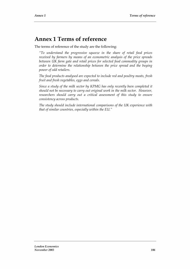
Annex 1 Terms of reference
Annex 1 Terms of reference The terms of reference of the study are the following:
“To understand the progressive squeeze in the share of retail food prices received by farmers by means of an econometric analysis of the price spreads between UK farm gate and retail prices for selected food commodity groups in order to determine the relationship between the price spread and the buying power of odd retailers.
The food products analysed are expected to include red and poultry meats, fresh fruit and fresh vegetables, eggs and cereals.
Since a study of the milk sector by KPMG has only recently been completed it should not be necessary to carry out original work in the milk sector. However, researchers should carry out a critical assessment of this study to ensure consistency across products.
The study should include international comparisons of the UK experience with that of similar countries, especially within the EU.”
London Economics November 2003 106

Annex 2 Data: sources and description
Annex 2 Data: sources and description
Data collection and description In this annex we describe the data sources for the farm gate prices and the retail prices and any adjustments made to the data.
Producer prices Our main source for monthly producer prices is the information provided by Eurostat’s New Chronos Database. The data from Eurostat are, in many cases, incomplete and this limits the scope of our analysis. In some cases a whole range of years is missing. In others, there are gaps for some months.
For the UK we used producer prices provided by Defra. For red meat producer prices we used the data from the Meat and Livestock Commission (MLC).
Retail prices For monthly retail prices we gathered information from different sources, such as ZMP, ILO, MLC, national statistical agencies, etc.
For the UK and Austria we were able to obtain directly average retail prices in level from the national statistical agencies.
For other countries, we contacted each country’s national statistical agency to obtain consumer price index (CPI) data. However, this created two problems. First, we found that many countries do not provide disaggregated price information for certain food categories. This is especially the case for the categories “fruits” and “vegetables”. The main implication of this is that, for some countries, the spread for certain products (e.g. carrots or onions) cannot be computed as the product information is aggregated in a broader category.
The second problem is that CPI data are expressed in index form and not in level form, which is the measure required for computing the farm-retail price spread.
We overcame this problem by combining these CPI data with information on the price level of a number of food items available from the ILO. The ILO collects such information to estimate each year the level of real wages in most countries. Food retail price series in level form can be generated by multiplying the CPI index series with the price level information from the ILO25 databank. Below, we provide more details on this data operation.
London Economics November 2003 107
25 No data is available for Germany from the ILO website. A series for German white bread is constructed using the same CPI method using a starting point price for April 2002 obtained from the consumer

Annex 2 Data: sources and description
Retail prices for red meat products (beef, lamb and pork) were obtained from the Meat and Livestock Commission (MLC) for France, Germany, Netherlands and Ireland. Danmarks Statistik (Statistics Denmark) and Central Statistics Office Ireland also provided some information on red meat prices.
In addition, the various ZMP 2002 market reviews provided information on various food retail prices (in levels) from April 1987 to December 2001.
Imputation of missing values For prices series with missing monthly values, we imputed the missing values through one of three different methods.
Where possible, we imputed the missing monthly value by taking an average of the price in the month preceding the missing observation and the price in the following month.
In cases where prices were missing for consecutive months in some year, the missing value for month m was imputed by applying an assumed percentage change from the previous month (m-1). The assumed percentage change was computed as an average of the percentage change from the same months (m-1 and m) in the previous and following year.
In cases where the previous method generated large jumps in the series, we simply repeated the value of the month preceding the missing observations.
Overall, only very few series were affected by missing values and number of data imputations never exceeds five per series.
Using data from the ILO As noted earlier, in many countries (such as Denmark, Spain, the Netherlands) detailed information on retail prices is only available in index form such as the retail price index. This index series is very useful for analysing the price evolution (growth) over the years of a certain product. However, it cannot be used directly in cases where we are interested in the level of the price such as in the cross-country comparison of spreads.
To construct a useful price series in level form we proceeded as follows:
• We gathered a retail price for each of the products from the International Labour Organization (ILO)26.
section of http://home.telebel.de.
26 The ILO OCTOBER INQUIRY requests information national average retail prices in October of each year for as many as possible of 93 items of food and drink. If national averages are not available, average prices may be provided separately for up to three major towns or regions. The prices reported should be, as far as possible, those used regularly for calculating consumer price indices. They should also refer to the normal retail prices actually paid by the consumer, including any related taxes, such as sales taxes or value-added taxes. See http://laborsta.ilo.org/applv8/data/tO2e.html for a complete definition of the Inquiry.
London Economics November 2003 108

Annex 2 Data: sources and description
• We then multiplied the October 1990 ILO price27, with the relevant CPI series provided by the national statistics offices28.
• Finally, these calculated retail food prices (in levels) were converted into euros by using the appropriate exchange rate.
The prices for red meat Monthly series for producer and retail prices were provided by the Meat and Livestock Commission (MLC) and CSO Ireland.
The producer price for the UK is derived from a survey of auctions or abattoirs and reflects the farm gate price of the livestock of interest. The retail UK prices series represents the average price of a basket of meat cuts taken from a sample of retail outlets. The prices series are expressed in carcase weight equivalent, so that farm and retail prices are fully comparable.
The MLC have also provided monthly retail prices for selected cuts of beef, pork and lamb for four EU countries: France, Germany, Netherlands (beef and pork only) and Ireland.
For all the countries, we have obtained retail prices for two meat cuts29, generally an “expensive” cut, such as “Sirloin steak”, and a “less expensive” cut, such as “Brisket“. In some cases the definition of one of the cuts was not constant over time, e.g. there was a new definition of the expensive cut after time t. The percentage increases of the newly defined series were used to expand the original series. In the year where the break takes place (t), the change in price from December to January was assumed to be zero.
The retail price was constructed by taking a weighted average of both prices using the relative weights of each cut. For EU countries other than the UK, we used the proportions of UK cuts, as shown in Table A.1. For some EU countries where retail prices were given for a different type of cut, such as “lamb gigot chops” in Ireland, we obtained the appropriate weights from the MLC. The average price is then multiplied by a factor representative of the useable proportion of the carcase (excluding bone, fat and trimmings) and by a factor allowing for drip loss. The corresponding adjustment factors are shown in Table A.2. We should note that this assumes that bone, fat and trimmings are assumed to have no value and that, due to data limitation, this price is only representative of a share of the total cattle or lamb.
27 In the case of Italy and the Netherlands where detailed CPI information is available only from 1996 onwards, the ILO price level for October 1996 was used to create the level series.
28 The CPI index series was re-based to October 1990 = 100 in this operation.
29 Except for Ireland where we obtained retail prices for four cuts with CSO Ireland providing prices for two additional cuts, and for German Lamb where only cut was recorded.
London Economics November 2003 109

Annex 2 Data: sources and description
Table A.1: Weight proportions of cuts
Beef % Lamb %
Topside 19.3 Whole leg 21.8
Rump steak 3.8 Loin chops 9.0
Sirloin steak 4.5 Cutlet chops 7.1
Fillet steak 1.4 Shoulder 21.8
Best braising steak 12.1 Leg steaks 6.4
Diced (stewing steak) 4.8 Diced lamb 9.6
Premium minced beef 13.8
Standard minced beef 10.3 Source: MLC.
Table A.2: Carcase and drip loss
Beef Lamb
Proportion of meat (excluding bone, fat and trimmings) 70.0 % 75.7%
Drip loss correction coefficient 95% 97% Source: MLC.
The farm gate prices also need to go through some transformation. First, prices need to be expressed in deadweight. For the EU countries where the MLC provided cattle prices in liveweight early in the time series (from 1985-1990) the series was extended back using monthly incremental percentage changes, again assuming no change between the December and January into the year of the break. For Ireland where all cattle prices were given in liveweight we needed to transform them into deadweight. We used the assumptions in Fowler and Sams (1999) that the average killing out percentage is 54% for cattle. Hence, these prices will need to be divided by 0.54.
In the case of German lamb we found that there was a significant and unexplainable break30 in the MLC retail price series. Therefore, a different retail series for German lamb was constructed using the CPI series for frozen lamb, by converting this index series into a price level series, using an average price for German lamb leg in 2000 from the MLC series.
30 No change in recording classification is listed in the MLC’s European Handbook nor is the MLC able to provide an explanation for this break.
London Economics November 2003 110

Annex 2 Data: sources and description
Prices for chicken Retail prices for chicken were obtained from different sources. Farm gate prices for chicken were obtained from Eurostat, except in the case of the UK where Defra data were used. For some EU countries, prices were only available in liveweight. In such cases, prices were converted deadweight (or carcase weight equivalent) by dividing by a percentage of 75%. This percentage has been obtained from MAFF (1999).
Products covered by the study As a result of our investigation we have been able to collect meaningful information for 12 agricultural products that yield 13 farm gate-retail price spreads (see Table A.3). We believe that these products should be representative of the different agricultural supply chains as explained in the table below.
Table A.3: Agricultural products and analysis of supply chain
Supply chain Agricultural/retail products
Cereals Wheat, Bread, Flour
Red meat Beef, Lamb
Poultry meats Chicken
Fresh fruit Apples, Pears (Germany only)
Fresh vegetables Potatoes, Onions, Carrots, Cabbage, Tomatoes
Eggs Eggs
Data availability by country
United Kingdom
Producer prices Farm prices were obtained from Eurostat for the following commodities (1985m1-2001m12): “Onions all qualities”, “White cabbage all qualities”, “Tomatoes under glass all qualities”, “Main crop potatoes”, “Carrots all qualities”, “Dessert apples all varieties”, “Chickens (class A; slaughtered) - prices per dead weight”.
Prices for “Soft wheat” are available from Eurostat. However, after discussions with HGCA, we were advised not to use that series because it is
London Economics November 2003 111

Annex 2 Data: sources and description
not representative of the type of wheat used for making UK bread and flour. We were informed that UK millers use a blend of various types of wheat, preferring harder wheats to soft ones31. Following HGCA’s advice, the farm gate price series was constructed as follows. We took the price of “Feed wheat” and added a premium to estimate a price for “Medium quality bread making wheat”. The premium has been computed as one half of the difference between “Breadmaking wheat” (which is representative of a high quality bread) and the “Feed wheat”. The prices of “Feed wheat” and “Breadmaking wheat” are available from DEFRA (as provided by HGCA). Hence, this estimated price for “Medium quality bread making wheat” should be a more realistic measure of bread wheat prices.
Farm prices were obtained from DEFRA for “Eggs (Size 3-intensive)”.
Data for “Beef Producer”, “Lamb Producer”, “Pig Producer” and “Bacon Producer” was obtained from the MLC.
Retail prices Average prices (in levels) were obtained from the ONS for the following commodities: “Flour self raising”, “Chicken roasting, oven ready, fresh/chilled”32, “Apples, dessert”, “Onions”, “Carrots”, “Cabbage”, “Tomatoes”, “Potatoes, old loose”.33 For eggs we use the price of “Eggs size 2 (65-70g)”.
As for bread, we used the price of “Bread white loaf, sliced”, which is the most common bread used in the UK.
Data for retail prices of red meat products (Beef, Lamb and Pork) were provided by the Meat and Livestock Commission (MLC).
Austria Farm prices were obtained from Eurostat for the following commodities (1985m1-2001m12): “Soft wheat”, “Main crop potatoes”, “White cabbage: all qualities”, “Tomatoes in the open: all qualities”, “Tomatoes under glass: all qualities”, “Carrots: all qualities”, “Onions: all qualities”, “Dessert apples: all varieties”, “Chickens (live; 1st choice) live weight”, “Chickens (class A; slaughtered) - dead weight”, and “Fresh eggs”.
31 This is not true for the rest of EU countries, which use mainly with soft wheat for their bread.
32 An RPI is also available for Chicken roasting, oven ready, frozen. We decided against using this price series because the British Poultry Council informed us that frozen chicken are mainly imported.
33 Retail prices for Apples, Onions, Carrots, Cabbage, Tomatoes, and Potatoes was provided in lb before February 1999. We converted the prices in pound into prices per kilogram by using the appropriate correction factor. Chicken prices were expressed in lb before February 1996 and the correspondent adjustment was also made.
London Economics November 2003 112

Annex 2 Data: sources and description
Average retail food prices (in level form) were obtained from Statistics Austria for the following commodities (1996m1-2002m12): “Roast chicken”, “White bread”, “Eggs”, “Apples”, “Carrots”, “White cabbage”, “Tomatoes”, “Onions”, and “Potatoes”.
Denmark Farm prices were obtained from Eurostat for the following commodities (1985m1-2001m12 except for eggs 1985m1-1996m12). “Soft wheat”, “Fresh eggs (whole country)”, “Main crop potatoes”, “Chickens (live; 1st choice)”.
Food CPI data were obtained from the Danish statistical agency for the following commodities (1996m1-2002m12): “Flour and grain”, “Bread”, “Cakes and biscuits”, “Poultry”, “Eggs”, “Fresh fruit”, “Fresh vegetables”, and “Potatoes”.
ILO prices were obtained for the following commodities: “Wheat bread”, “Wheat flour”, “Chicken eggs”, “Potatoes”34 (see Table A.4 for a definition). A retail price was constructing by using the ILO values for October 1990.
34 The ILO price for Chicken was not available.
London Economics November 2003 113

Annex 2 Data: sources and description
Table A.4: ILO definitions table
Wheat Bread Wheat bread, white, unsliced, not wrapped 500g: (b) white, unsliced, not wrapped 500g Ordinary bread, prepared from 100 per cent white wheat flour, most commonly sold variety, fresh, unsliced, not wrapped. Excluded: French “baguette” type.
Bread “baguette” French “baguette” type prepared from 100 per cent white wheat flour, fresh, unsliced, not wrapped. Excluded: Specially flavoured types and those with seeds (such as sesame) on top.
Wheat Flour Wheat flour, white 1kg: All-purpose white wheat flour, in most commonly sold packaging, may be vitamin enriched. Excluded: Self-raising types.
Chicken Chicken, cleaned 1kg: Whole chicken, cleaned, without head and feet, but may include heart, liver and gizzard. Price fresh or frozen, whichever most commonly sold and specify.
Chicken Eggs Chicken eggs, fresh 12 eggs: Either brown or white, weight per egg approximately 60 grams, may be sold in cartons of 6, 10 or 12 or sold unpackaged. Excluded: Eggs with cracked or broken shells, and any type of preserved eggs.
Potatoes Potatoes, any variety, including red skinned potatoes if interior is white. Excluded: Sweet potatoes and yams.
France Farm prices were obtained from Eurostat for the following commodities (1985m1-2002m6) “Soft wheat”, “Onions: all qualities”, “Chickens (live; all qualities)”, “Chickens (live; 1 choice)” Fresh Eggs.
CPI were obtained from INSEE for “Eggs”, “Poultry” and “Bread”. ILO prices were obtained for the “Eggs”, “Chicken” and “Bread” (see Table A.4). Food retail price data were constructing by multiplying the CPI series with the respective ILO data points of October 1993 (the earliest available data).
Germany Farm gate prices were obtained from Eurostat for the following commodities (1985m1-2001m12): “Onions: all qualitities”, “ Soft Wheat”, “Chickens (class A; slaughtered) - dead weight”, “Fresh Eggs”, “Carrots all qualities”, “Main Crop Potatoes”, “White Cabbage all qualities”, “Tomatoes under glass: all qualities”. London Economics November 2003 114

Annex 2 Data: sources and description
Farm gate prices were obtained from ZMP (1985m1-2002m12) for “Apples (Golden Delicious”, “Apples (Jonagold)”, and “Pears”.
Average retail prices were obtained from ZMP for the following commodities (1985m1-2003m9): Onions”, “Chicken (fresh)”, “Eggs”, “Carrots”, “Potatoes”, “White Cabbage”, “Apples (Golden Delicious)”, “Apples (Jonagold)”, “Pears” and “Tomatoes”.
The series for consumer lamb, as provided by the MLC, showed an unexplainable break for the year 1998 and we decided to exclude it from the analysis. A different retail series for German lamb was constructed using the CPI series for “Frozen Lamb” and converting this index series into a price level series by using the average price for German lamb leg in 2000 from the MLC series.
The “White Bread” CPI retail food price indices were obtained from Statistics Germany. To construct the series in levels, a price for “White Bread 500g (2002m4)” was obtained from the Consumer News section of http://home.telebel.de.
Netherlands Farm prices were obtained from Eurostat for the following commodities (1985m1-2001m12): “Soft wheat”, “Chickens (live; 1st choice)”, “Fresh eggs (whole country)”, and “Main crop potatoes”.
Food CPI data were obtained from Statistics Netherlands for the following commodities (1996m1-2002m12): “Bread and cereals”, “Poultry”, “Fresh fruit”, “Dried fruit and nuts”, “Vegetables”, “Potatoes, other tubers”, “Fresh vegetables”, “Potatoes”, and “Eggs”.
ILO prices were obtained for “Wheat bread”, “Chicken eggs”, and “Potatoes” (see Table A.4). Food retail price data were constructing by multiplying the CPI series with the respective ILO data points of October 1996.
Ireland Farm prices were obtained from Eurostat for the following commodities (1985m1-2001m12) “Onions all qualities”, “Soft Wheat”, “Fresh Eggs”, “Tomatoes under glass: all qualities”, “Carrots all qualities”.
Average prices (in level form) were obtained from CSO Ireland for “Onions”, “Tomatoes”, “Carrots”, “Eggs” and “White Bread”.
Italy Farm prices were obtained from Eurostat for the commodities (1985m1-1999m12): “Soft wheat”, “Main crop potatoes”, “Chickens (live; 1st choice)”, “Chickens (class A; slaughtered)” and “Fresh eggs (whole country)”.
London Economics November 2003 115

Annex 2 Data: sources and description
CPI was obtained from ISTAT for the following commodities (1996m1-2002m12): “Bread and cereals”, “Bread”, “Flour”, “Bakery products”, “Biscuits”, “Other cereals and prepared dishes”, “Poultry”, “Eggs”, “Fruit”, “Fresh fruit”, “Vegetables”, and “Fresh vegetables legumes and potatoes”.
The ILO prices were obtained for: “Wheat bread”, “Wheat flour”, “Chicken”, and “Chicken eggs” (see Table A.4). The data includes three separate price series for Milan, Naples and Rome. Because CPI data are available only since 1996, a retail price was constructed by averaging the three values for October 1996.
Spain Farm prices were obtained from Eurostat for the following commodities (1985m1-2001m12): “Soft wheat”, “Main crop potatoes”, “Chickens (live; 1st choice)”, “Chickens (class A; slaughtered)”, “Fresh eggs”.
Food CPI data were obtained from INE for the following commodities (1985m8-2001m12): “Bread”, “Potatoes”, and “Eggs”.
ILO prices were obtained for the following commodities: “Bread baguette”, “Chicken eggs”, and “Potatoes”. A retail price was constructing by using the ILO values for October 1990.
Summary of data collection Finally, Table A.5 presents a summary overview of the various farm gate-retail price spreads for which we have found useful data and the period over which the data are available.
Altogether we have data on 60 different farm gate–retail price spreads in 9 different EU Member States.
London Economics November 2003 116

Annex 2 Data: sources and description
Table A.5: Availability of farm gate-retail price spreads
Agricultural sector Spread Countries
Wheat/bread United Kingdom (1987-2001)
Austria (1994-2002)
Denmark (1985-2000)
France (1990-2002)
Germany (1991-2002)
Ireland (1989-2001)
Italy (1996-2000)
Netherlands (1996-2001)
Spain (1989-2001)
Cereals
Wheat/flour United Kingdom (1987-2001)
Austria (1994-2002)
Denmark (1985-2000)
Italy (1996-2000)
Beef United Kingdom (1986-2003)
France (1987-2003)
Germany (1986-2002)
Ireland (1989-2002)
Netherlands (1994-2002)
Pork United Kingdom (1986-2003)
France (1989-2003)
Germany (1989-2001)
Ireland (1989-2001)
Netherlands (1989-2002)
Red Meat
Lamb United Kingdom (1986-2003)
France (1987-2001)
Germany (1991-2003)
Ireland (1989-2003)
Poultry meats Chicken United Kingdom (1987-2001)
France (1990-1998)
Germany (1993-2002)
Italy (1996-1999)
Netherlands (1996-2001)
London Economics November 2003 117

Annex 2 Data: sources and description
Table A.5: Availability of farm gate-retail price spreads
Agricultural sector Spread Countries
Fresh fruit Apples United Kingdom (1987-2001)
Austria (1997-2002)
Germany (1987-2003)
Pears Germany (1987-2003)
Potatoes United Kingdom (1985-2001)
Austria (1994-2002)
Denmark (1985-2000)
Germany (1993-2002)
Netherlands (1985-2001)
Spain (1985-2001)
Onions United Kingdom (1987-2001)
Austria (1997-2002)
Germany(1993-2001)
Carrots United Kingdom (1987-2001)
Austria (1997-2002)
Germany (1993-2001)
Cabbage United Kingdom (1987-2001)
Austria (1997-2002)
Germany (1993-2001)
Fresh vegetables
Tomatoes United Kingdom (1987-2001)
Germany (1998-2001)
Eggs Eggs United Kingdom (1992-2001)
Denmark (1985-1996)
France (1990-2002)
Germany (1993-2002)
Ireland (1989-2001)
Italy (1996-2000)
Netherlands (1990-2002)
Spain (1985-2001)
London Economics November 2003 118

Annex 3 Cross-country comparisons of farm gate-retail price spreads
Annex 3 Cross-country comparisons of farm gate-retail price spreads
To compare the evolution over time and across countries of the various spreads, for each commodity, we plot the spreads expressed as a percentage of the farm gate price (spread ratio) indexed to UK spread ratio in January 1990. We also provide information on the correlation between the UK farm gate-retail price spread and the similar spread in other EU Member States.
For each group of products, the correlations are computed over the periods for which observations are available for all the countries. This remark applies to all products except for the red meats. In the latter case, because data for Ireland is provided only every 4 months before 1997, the correlations are computed pair wise between each country and the UK.
Beef Beef price spreads in France, Germany and the Netherlands increased significantly by more than in the United Kingdom and Ireland (Figure A.1). A correlation analysis of the beef spreads in various EU Member States with the beef spread in the United Kingdom supports this conclusion as only the beef spread in Ireland shows a high correlation with the beef spread in the United Kingdom (Table 1.2).
Figure A.1: Beef price spreads
0.5
11
.52
2.5
33
.54
4.5
5S
prea
d R
atio
1990m1 1992m1 1994m1 1996m1 1998m1 2000m1 2002m1 2004m1Time(months)
UK FranceGermany IrelandNetherlands
Beef
London Economics November 2003 119

Annex 3 Cross-country comparisons of farm gate-retail price spreads
Table A.6: Correlation of Beef Spread Ratios between European countries and the United Kingdom
Country Correlation Coefficient
France 0.58
Germany 0.46
Ireland 0.80
Netherlands 0.42
Lamb In contrast, the UK lamb price spreads appears to have risen the most in the United Kingdom out of the four EU Member States for which we have information and only Ireland appears to exhibit to a similar, albeit less pronounced, trend (Figure A.2 and Table A.7)
Figure A.2: Lamb price spreads
0.5
11.
52
2.5
3Sp
read
Rat
io
1990m1 1992m1 1994m1 1996m1 1998m1 2000m1 2002m1 2004mTime(months)
1
UK FranceGermany Ireland
Lamb
London Economics November 2003 120

Annex 3 Cross-country comparisons of farm gate-retail price spreads
Table A.7: Correlation of Lamb Spread Ratios between European Countries and the United Kingdom
Country Correlation Coefficient
France 0.18
Germany -0.08
Ireland 0.70
Pork In sharp contrast to the patterns observed for beef and lamb price spreads, the pork price spreads appear to move relatively in tandem across all EU Member States, with the spreads in all EU Member States showing a relatively high correlation with the spread in the United Kingdom (Figure A.3 and Table A.8).
Figure A.3: Pork price spreads
0.5
11.
52
2.5
33.
5Sp
read
Rat
io
1990m1 1992m1 1994m1 1996m1 1998m1 2000m1 2002m1 2004m1Time(months)
UK FranceGermany IrelandNetherlands Denmark
Pork
London Economics November 2003 121

Annex 3 Cross-country comparisons of farm gate-retail price spreads
Table A.8: Correlation of Pork Spread Ratios between European Countries and the United Kingdom
Country Correlation Coefficient
France 0.57
Germany 0.62
Ireland 0.72
Netherlands 0.72
Denmark 0.64
Chicken The overall picture is one of relatively little change in spreads over time, although certain periods are characterised by sharp upward or downward spikes in spreads. Movements in chicken price spreads are largely uncorrelated across countries.
Figure A.4: Chicken price spreads
0.5
11.
52
2.5
3Sp
read
Rat
io
1990m1 1992m1 1994m1 1996m1 1998m1 2000m1 2002m1 2004m1Time(months)
UK FranceGermany NetherlandsAustria Italy
Chicken
London Economics November 2003 122
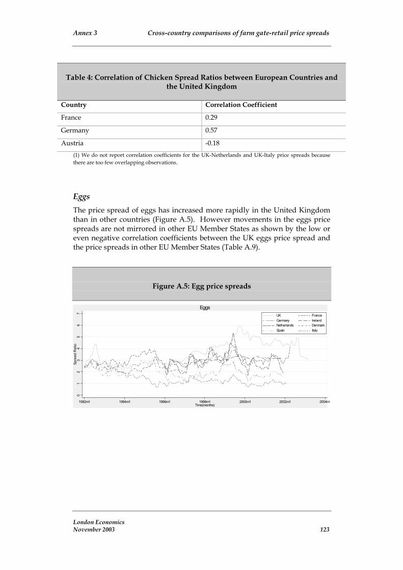
Annex 3 Cross-country comparisons of farm gate-retail price spreads
Table 4: Correlation of Chicken Spread Ratios between European Countries and the United Kingdom
Country Correlation Coefficient
France 0.29
Germany 0.57
Austria -0.18
(1) We do not report correlation coefficients for the UK-Netherlands and UK-Italy price spreads because there are too few overlapping observations.
Eggs The price spread of eggs has increased more rapidly in the United Kingdom than in other countries (Figure A.5). However movements in the eggs price spreads are not mirrored in other EU Member States as shown by the low or even negative correlation coefficients between the UK eggs price spread and the price spreads in other EU Member States (Table A.9).
Figure A.5: Egg price spreads
01
23
45
67
Spre
ad R
atio
1992m1 1994m1 1996m1 1998m1 2000m1 2002m1 2004m1Time(months)
UK FranceGermany IrelandNetherlands DenmarkSpain Italy
Eggs
London Economics November 2003 123

Annex 3 Cross-country comparisons of farm gate-retail price spreads
Table A.9: Correlation of egg price spreads between European countries and the United Kingdom
Country Correlation Coefficient
France -0.38
Germany -0.11
Ireland 0.13
Netherlands -0.52
Spain -0.73
Denmark 0.30
Italy 0.26
Wheat/bread The UK Wheat/bread price spread has increased less than in other countries, but movements in the spreads in the UK are correlated with those in about all other EU Member States in our sample. (Figure A.6 and Table A.11).
Figure A.6: Wheat/bread price spreads
34
56
78
910
1112
1314
Spre
ad R
atio
1990m1 1992m1 1994m1 1996m1 1998m1 2000m1 2002m1 2004m1Time(months)
UK FranceDenmark Spain
Wheat Bread
London Economics November 2003 124

Annex 3 Cross-country comparisons of farm gate-retail price spreads
Table A.10: Correlation of Wheat/bread Spread Ratios between European Countries and the United Kingdom
Country Correlation Coefficient
France 0.66
Ireland 0.56
Netherlands 0.60
Austria 0.51
Denmark 0.62
Spain 0.72
Italy 0.84
Wheat/flour The UK wheat price spread has increased less than in Austria and by about the same amount as in Denmark (Figure A.7). However, movements in spreads are correlated across countries (Table A.11).
Figure A.7: Wheat/flour price spreads
01
23
45
67
8Sp
read
Rat
io
1990m1 1992m1 1994m1 1996m1 1998m1 2000m1 2002m1 2004mTime(months)
1
UK AustriaDenmark Italy
Wheat Flour
London Economics November 2003 125

Annex 3 Cross-country comparisons of farm gate-retail price spreads
Table A.11: Correlation of Wheat/flour price spreads between European countries and the United Kingdom
Country Correlation Coefficient
Austria 0.76
Denmark 0.80
Italy 0.82
Potatoes The potatoes spread increased the most in the United Kingdom (Figure A.8), movements in UK potatoes price spreads are correlated with the Netherlands (Table A.12).
Figure A.8: Potatoes price spreads
01
23
45
67
89
1011
1213
Spre
ad R
atio
1990m1 1992m1 1994m1 1996m1 1998m1 2000m1 2002m1 2004m1Time (months)
UK DenmarkNetherlands Spain
Potatoes
Table A.12: Correlation of Potato price spreads between European countries and the United Kingdom
Country Correlation Coefficient
Netherlands 0.71
Denmark 0.53
Spain 0.41
London Economics November 2003 126

Annex 3 Cross-country comparisons of farm gate-retail price spreads
Onions Movements in the Onions price spreads of Ireland and Austria are to some extent correlated with those in the United Kingdom (Figure A.9 and Table A.13).
Figure A.9: Onions price spreads
01
23
45
67
8Sp
read
Rat
io
1993m1 1995m1 1997m1 1999m1 2001m1 2003mTime(months)
1
UK GermanyIreland Austria
Onions
Table A.13: Correlation of Onion price spreads between European countries and the United Kingdom
Country Correlation Coefficient
Germany 0.18
Ireland 0.67
Austria 0.62
Carrots A general downward trend in carrot spreads is apparent. The spreads also exhibit high volatility. UK carrots price spreads are highly correlated with those of Ireland but not with those of Germany and Austria.
London Economics November 2003 127

Annex 3 Cross-country comparisons of farm gate-retail price spreads
Figure A.10: Carrots price spreads
01
23
45
6Sp
read
Rat
io
1993m1 1995m1 1997m1 1999m1 2001m1 2003m1Time(months)
UK GermanyIreland Austria
Carrots
Table A.14: Correlation of carrots price spreads between European countries and the United Kingdom
Country Correlation Coefficient
Germany 0.34
Ireland 0.71
Austria 0.26
Cabbage The level of UK and German cabbage spreads differ markedly but both show a trend decline.
London Economics November 2003 128

Annex 3 Cross-country comparisons of farm gate-retail price spreads
Figure A.11: Cabbage price spreads
01
23
45
67
89
Spre
ad R
atio
1993m1 1995m1 1997m1 1999m1 2001m1 2003mTime(months)
1
UK GermanyAustria
Cabbage
Apples The apples price trends do not exhibit any strong trends, but are market by high volatility. Moreover, movements in UK apple price spreads are uncorrelated with those in Austria and Germany.
Figure A.12:Apples price spread
0.5
11.
52
2.5
33.
54
4.5
5Sp
read
Rat
io
1990m1 1992m1 1994m1 1996m1 1998m1 2000m1 2002m1 2004mTime(months)
1
UK GermanyAustria
Apples
London Economics November 2003 129
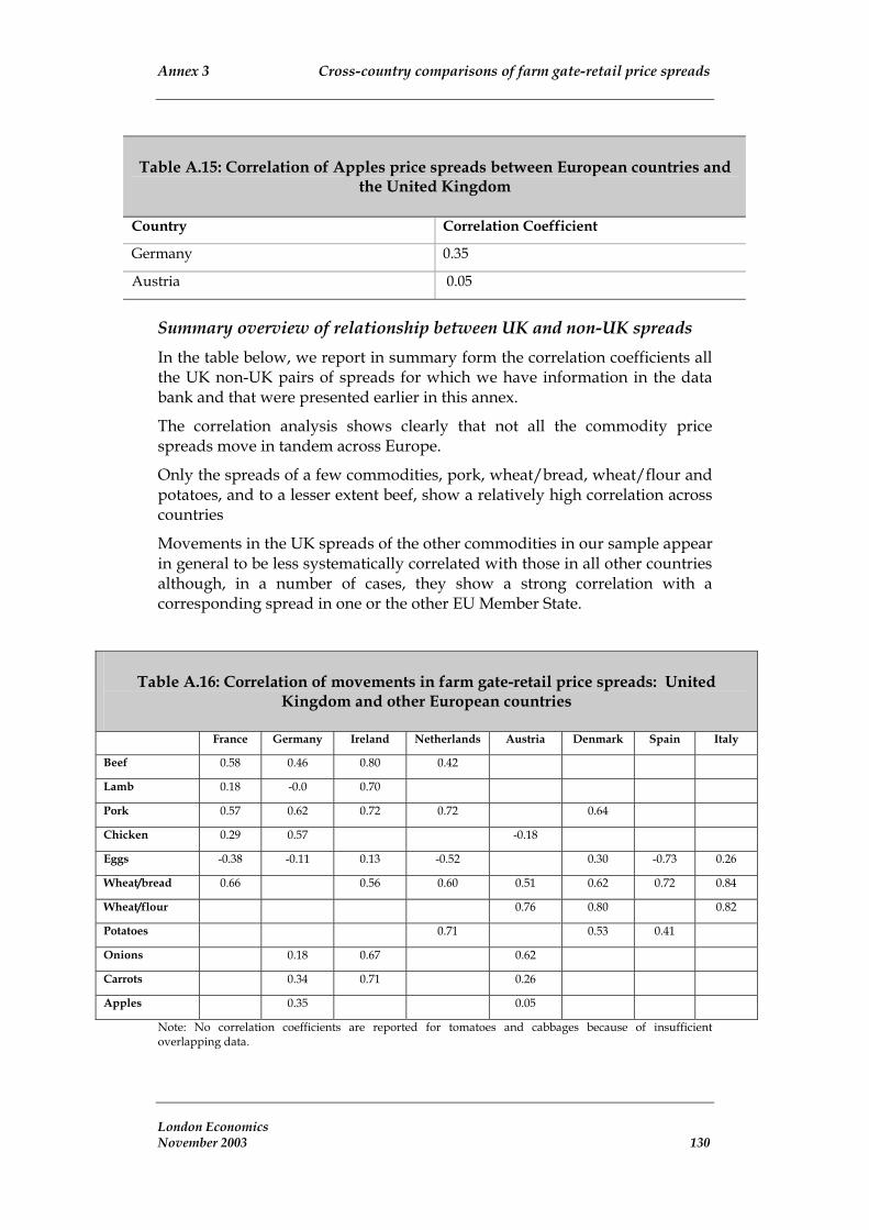
Annex 3 Cross-country comparisons of farm gate-retail price spreads
Table A.15: Correlation of Apples price spreads between European countries and the United Kingdom
Country Correlation Coefficient
Germany 0.35
Austria 0.05
Summary overview of relationship between UK and non-UK spreads In the table below, we report in summary form the correlation coefficients all the UK non-UK pairs of spreads for which we have information in the data bank and that were presented earlier in this annex.
The correlation analysis shows clearly that not all the commodity price spreads move in tandem across Europe.
Only the spreads of a few commodities, pork, wheat/bread, wheat/flour and potatoes, and to a lesser extent beef, show a relatively high correlation across countries
Movements in the UK spreads of the other commodities in our sample appear in general to be less systematically correlated with those in all other countries although, in a number of cases, they show a strong correlation with a corresponding spread in one or the other EU Member State.
Table A.16: Correlation of movements in farm gate-retail price spreads: United Kingdom and other European countries
France Germany Ireland Netherlands Austria Denmark Spain Italy
Beef 0.58 0.46 0.80 0.42
Lamb 0.18 -0.0 0.70
Pork 0.57 0.62 0.72 0.72 0.64
Chicken 0.29 0.57 -0.18
Eggs -0.38 -0.11 0.13 -0.52 0.30 -0.73 0.26
Wheat/bread 0.66 0.56 0.60 0.51 0.62 0.72 0.84
Wheat/flour 0.76 0.80 0.82
Potatoes 0.71 0.53 0.41
Onions 0.18 0.67 0.62
Carrots 0.34 0.71 0.26
Apples 0.35 0.05
Note: No correlation coefficients are reported for tomatoes and cabbages because of insufficient overlapping data.
London Economics November 2003 130

Annex 4 Detailed information on retail food industry in Europe
Annex 4 Detailed information on retail food industry in Europe
In this annex, we provide detailed information about the changes in the structure of the European retail food industry,
We begin by providing a short overview of the determinants of the customers’ choice of a specific food retail outlet. Next, we present some facts about the size distribution of food retail stores in Europe. This is followed by a country-by-country overview of major food retailers and their market share. We then review the financial performance of European food retail industry and present some facts about the key structural features of the UK food retail market.
Factors affecting the customer choice of a grocery store Retailers do not sell a homogeneous good. In fact the “product” they offer to their consumers is a rather complex one. It incorporates various types of services (e.g. parking facilities, in-store staff, etc.) and it also differs according to the actual range of products on the shelves. There are groups of retailers, though, for which these variables are more or less homogeneous, for example supermarkets and hypermarkets.
Nevertheless there is one variable in particular that does not allow treating retailers as sellers of a homogeneous good: stores location. According to numerous surveys, what is by far the most important reason for shopping at a particular outlet is not whether prices are lower or the staff is friendlier but simply where the shops are located in relation to the clients’ homes or workplaces.
For example, in its recent enquiries into the Safeway merger, the UK Competition Commission has relied on the assumption that consumers will on average be unwilling to travel more than 10 or 15 minutes (for urban and rural areas, respectively) to look for alternative food retailers.
Table A.17: Factors affecting the choice of grocery store
Most important factor Proportion of respondents
Convenience 54
Product range/selection 14
Low price 13
Quality 9
London Economics November 2003 131
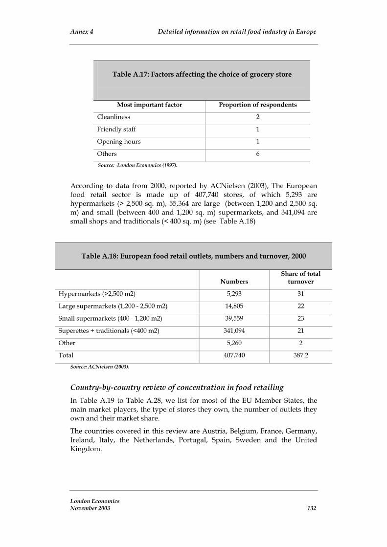
Annex 4 Detailed information on retail food industry in Europe
Table A.17: Factors affecting the choice of grocery store
Most important factor Proportion of respondents
Cleanliness 2
Friendly staff 1
Opening hours 1
Others 6
Source: London Economics (1997).
According to data from 2000, reported by ACNielsen (2003), The European food retail sector is made up of 407,740 stores, of which 5,293 are hypermarkets (> 2,500 sq. m), 55,364 are large (between 1,200 and 2,500 sq. m) and small (between 400 and 1,200 sq. m) supermarkets, and 341,094 are small shops and traditionals (< 400 sq. m) (see Table A.18)
Table A.18: European food retail outlets, numbers and turnover, 2000
Numbers Share of total
turnover
Hypermarkets (>2,500 m2) 5,293 31
Large supermarkets (1,200 - 2,500 m2) 14,805 22
Small supermarkets (400 - 1,200 m2) 39,559 23
Superettes + traditionals (<400 m2) 341,094 21
Other 5,260 2
Total 407,740 387.2
Source: ACNielsen (2003).
Country-by-country review of concentration in food retailing In Table A.19 to Table A.28, we list for most of the EU Member States, the main market players, the type of stores they own, the number of outlets they own and their market share.
The countries covered in this review are Austria, Belgium, France, Germany, Ireland, Italy, the Netherlands, Portugal, Spain, Sweden and the United Kingdom.
London Economics November 2003 132

Annex 4 Detailed information on retail food industry in Europe
Table A.19: Austria: Main food retailers 2001-2002
Group Operations No. of outlets Mkt. share
BML (Rewe Germany) Supermarkets 1248 31.0%
Spar
Hypermarkets/supermarkets discount stores 1499 28.5%
Hofer Discount stores 230 14.0%
ADEG Wholesale and retail group 751 9.4%
Zielpunkt Discount stores 293 4.5%
Lidl (Germany) Discount stores 56 2.7%
M-Preis Supermarkets 107 2.4%
Maximarkt Hypermarkets 6 1.4%
Unimarkt (Pfeiffer) Supermarkets 56 1.2%
Nah & Frisch Supermarkets 152
not recorded (estimate) 5%
Source: Mintel 2002.
Table A.20: Belgium: Main food retailers 2001-2002
Group Operations No. of outlets Mkt. share
Carrefour (France)
Hypermarkets/ supermarkets /food stores 129 25.3%
Delhaize Group Food & non-food outlets 675 21.8%
Colruyt Discount supermarkets 159 16.0%
Louis Delhaize
Hypermarkets/supermarkets discount stores 717 9.1%
Aldi (Germany) Discount food stores 335 8.4%
Laurus (Netherlands) Supermarkets 481 4.1%
London Economics November 2003 133

Annex 4 Detailed information on retail food industry in Europe
Table A.20: Belgium: Main food retailers 2001-2002
Group No. of outlets Mkt. share Operations
Mestdagh (France 25%) Supermarkets 61 2.7%
Lidl (Germany) Discount food stores 120
Intermarche (France) Supermarkets /hypermarkets
1.6%
60 1.1%
Franchised supermarkets / superettes Lambrechts 230 0.7%
Delto Supermarkets 315
Prima Supermarkets 250
Tecno Supermarkets 90
Automated food store Shop 24 60
Covee Supermarkets 55
O'Cool Frozen food shops 42
not recorded (estimate) 10%
Source: Mintel 2002.
Table A.21: France: Main food retailers 2001-2002
Group Operations No. of outlets Mkt. share
Carrefour Food multiple 3196 21.6%
Intermarche Voluntary Group 3698 13.7%
Leclerc Voluntary Group 541 12.3%
Auchan Food multiple 361 9.5%
Casino Supermarkets 5809 9.1%
Systeme U Food buying group 819 6.0%
Schiever Food multiple 195 3.4%
Cora Food multiple 203 3.4%
Co-op Atlantique Food co-operative 281 2.9%
Co-op Normandie Picardie Food co-operative 420 2.7%
Co-op Alsace Food co-operative 145 2.3%
London Economics November 2003 134

Annex 4 Detailed information on retail food industry in Europe
Table A.21: France: Main food retailers 2001-2002
Lidl (Germany) Discount food stores 948
Aldi (Germany) Discount food stores 440
Penny (Germany) Discount food stores
not recorded (estimate) 15%
Source: Mintel 2002.
Table A.22: Germany: Main food retailers 2001-2002
Group Operations No. of outlets Mkt. share
Edeka\AVA Gruppe Voluntary Group 10244 26.3%
Rewe Food group 7326 16.1%
Aldi Discount food stores 3532 15.6%
Schwarz Gruppe Discount food stores & hypermarkets 2360 11.1%
Metro Hypermarkets & superstores 746 8.5%
Spar (France) Food group 4328 7.4%
Tengelmann Food group 3420 6.4%
Globus Hypermarkets 35 2.7%
Wal-Mart (USA) Hypermarkets 95 2.4%
Norma\Rodi Discount food stores 1150 1.8%
Dohl Gruppe Voluntary co-operative 200 1.7%
Source: Mintel 2002.
Table A.23: Ireland: Main food retailers 2001-2002
Group Operations No. of outlets Mkt. share
Musgrave Voluntary chain 560 31.6%
Tesco (UK) Supermarkets & discount food stores 76 21.4%
Dunnes Stores Supermarkets & general goods 80 14.5%
Superquinn Superstores 19 12.9%
London Economics November 2003 135

Annex 4 Detailed information on retail food industry in Europe
Table A.23: Ireland: Main food retailers 2001-2002
BWG Foods Voluntary chain & cash & carries 362 9.5%
ADM Londis Buying group/ Voluntary chain 237 5.3%
John Pettitt Supermarkets 25
Costcutter Voluntary group 67
Vivo Voluntary group 50
Tony Quinn health stores Health foods 13
Lidl (Germany) Discount stores 10
Barryroe Co-operative Ltd Co-op 9
TF Fleming Ltd Supermarkets 8
Greens Food Fare Supermarkets na
L & N Ltd Supermarkets na
J. O'Connor Supermarkets na
not recorded (estimate) 5%
Source: Mintel 2002.
Table A.24: Italy: Main food retailers 2001-2002
Group Operations No. of outlets Mkt. share
Co-op Italia Co-operative group 1085 19.4%
Conad Buying group 3140 17.0%
Carrefour (France) Hypermarkets 905 16.5%
Gruppo Rinascente (France)
Hypermarkets / Supermarkets 227 12.1%
Esselunga Supermarkets 112 7.8%
Despar Italia Voluntary chain 1664 6.4%
Rewe (Germany) Food stores 344 3.9%
Finiper Hypermarkets 20 3.6%
Gruppo Lombardini Supermarkets & discount food stores 401 3.4%
Nuova Distribuzione Supermarkets 160 3.2%
London Economics November 2003 136
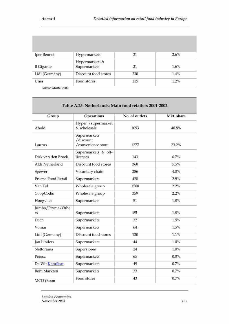
Annex 4 Detailed information on retail food industry in Europe
Table A.24: Italy: Main food retailers 2001-2002
Iper Bennet Hypermarkets 31 2.6%
Il Gigante Hypermarkets & Supermarkets 21 1.6%
Lidl (Germany) Discount food stores 230 1.4%
Unes Food stores 115 1.2%
Source: Mintel 2002.
Table A.25: Netherlands: Main food retailers 2001-2002
Group Operations No. of outlets Mkt. share
Ahold Hyper /supermarket & wholesale 1693 40.8%
Laurus
Supermarkets /discount /convenience store 1277 23.2%
Dirk van den Broek Supermarkets & off-licences 143 6.7%
Aldi Netherland Discount food stores 360 5.5%
Spewer Voluntary chain 286 4.0%
Prisma Food Retail Supermarkets 428 2.5%
Van Tol Wholesale group 1500 2.2%
CoopCodis Wholesale group 359 2.2%
Hoogvliet Supermarkets 51 1.8%
Jumbo/Pryma/Others Supermarkets 85 1.8%
Deen Supermarkets 32 1.5%
Vomar Supermarkets 64 1.5%
Lidl (Germany) Discount food stores 120 1.1%
Jan Linders Supermarkets 44 1.0%
Nettorama Superstores 24 1.0%
Poiesz Supermarkets 65 0.8%
De Wit Kom@art Supermarkets 49 0.7%
Boni Markten Supermarkets 33 0.7%
MCD (Boon Food stores 43 0.7%
London Economics November 2003 137

Annex 4 Detailed information on retail food industry in Europe
Table A.25: Netherlands: Main food retailers 2001-2002
Group Operations No. of outlets Mkt. share
Sliedrecht)
EM –TE Supermarkets 22 0.5%
Source: Mintel 2002.
Table A.26: Portugal: Main food retailers 2001-2002
Group Operations No. of outlets Mkt. share
Modelo Continente Grocery Food stores 101 26.0%
Jerónimo Martins Hypermarkets & supermarkets 236 19.6%
Intermarche (France) Hypermarkets & supermarkets 165 10.8%
Carrefour (France) Food stores 331 10.7%
Jumbo (France) Hypermarkets 14 9.6%
Makro (Germany) Cash & carries 9 9.0%
Grula Co-operative food group 371 2.9%
Alisuper Franchised supermarkets 230 0.7%
group 27 0.5%
Novimundo Food group na 0.4%
AC Santos Food group 21 0.3%
Supermercados Ulmar Food group na 0.3%
Agora Supermercados Food group na 0.1%
Food group na 0.1%
Lidl (Germany) Discount food stores 145
Leclerc (France) Hypermarkets 9
not recorded (estimate) 10%
Pluricoop Food
Geneco
Source: Mintel 2002.
London Economics November 2003 138

Annex 4 Detailed information on retail food industry in Europe
Table A.27: Spain: Main food retailers 2001-2002
Group Operations No. of outlets Mkt. share
Carrefour (France) Grocery multiple 2669 30.9%
Grupo Eroski Retail / co-operative group 1460 12.8%
Mercadona Supermarkets 589 12.6%
Auchan (France) Grocery multiple 150 9.6%
El Corte Ingles Supermarkets within department stores 63 8.1%
Superdiplo (Netherlands) Grocery multiple 623 5.9%
Caprabo Supermarkets 477 4.4%
El Arbol, Superspar (Netherlands) Supermarkets 610 2.5%
Lidl (Germany) Discount food stores 340 2.0%
Gadisa Supermarkets / cash and carry 232 1.9%
Grupo Ahorramus Supermarkets 153 1.9%
Miquel Alimentacion Grupo Discount food stores 139 1.5%
Condis Supermercats Supermarkets 160 1.3%
Vegalsa Supermarkets 475 1.2%
Supermarket Alcosto Supermarkets 56 1.0%
Grupo Enaco Supermarkets /cash and carry 76 0.9%
Plus Espana (Germany) Discount food stores 152 0.8%
Dialsur ( Ireland) Supermarkets 37 0.4%
ITM iberica ( France) Supermarkets 90 0.1%
Hyper L (Leclerc France) Hypermarkets 6 0.1%
Dunnes (Ireland) Supermarkets 4 0.0%
Source: Mintel 2002.
London Economics November 2003 139

Annex 4 Detailed information on retail food industry in Europe
Table A.28: UK: Main food retailers 2001-2002
Group Operations No. of outlets Mkt. share
Tesco na 728 23.8%
Sainsbury's na 463 16.5%
ASDA (Wal-Mart USA) na 250 12.6%
Safeway na 484 9.9%
Somerfield na 1300 5.5%
Wm Morrison na 113 4.7%
Co-operative Group na 1071 2.9%
Waitrose na 136 2.6%
Spar na 2591 2.1%
Iceland na 766 1.9%
Londis na 2065 1.4%
Aldi (Germany) na 250 1.2%
Costcutter na 1050 1.1%
Shell na 1070 0.8%
United Norwest C-op na 453 0.7%
Lidl (Germany) na 250 0.7%
BP Amoco na 1500 0.6%
Alldays na 774 0.6%
Esso na 1460 0.6%
Netto (Denmark) na 123 0.6%
not recorded (estimate) 10.0%
Source: Mintel 2002.
Performance Indicators of performance are an important set of indicators of the market power of food retailers. In principle we would expect to see retailers in concentrated markets perform better, in terms of profits, for example, than retailers in very competitive markets. A particularly useful indicator of performance (and expected performance) for listed companies is their stock price. The stock price evolution should mirror investors’ perceptions of current and future profit opportunities for the underlying company.
London Economics November 2003 140

Annex 4 Detailed information on retail food industry in Europe
In the figure below, we see that the evolution of an EU-wide index of stock prices of retailers has been less favourable than the performance of the general index. This can be taken as an indicator that the market does not perceive this sector to be likely to attain above average profit performance.
Figure A.13: Share price performance: food retailers in the EU
The table below (Table A.29) breaks down some of the information above on a country-by-country basis. The changes in food retailers’ share prices, in the three years to January 2001, have differed significantly across countries. In the period, there were very large gains in France and Italy and a very substantial loss in Germany.
London Economics November 2003 141

Annex 4 Detailed information on retail food industry in Europe
Table A.29: Stock market performance of food and drug retailers
Share price 1-Jan-98
Share price 31 – Jan -01
% Change
United Kingdom 1,000 1,128 12.8
France 1,000 1,815 81.5
Germany 1,000 405 -59.5
Spain 1,000 1,023 2.3
Italy 1,000 1,495 49.5
Netherlands 1,000 1,335 33.5
Analysis of the UK market In the UK, hypermarkets carry a very important weight in total food retailing sales and this trend has accentuated in recent years.
Figure A.14: UK grocery trade, shop number by type
Source: ACNielsen ( 2003).
London Economics November 2003 142
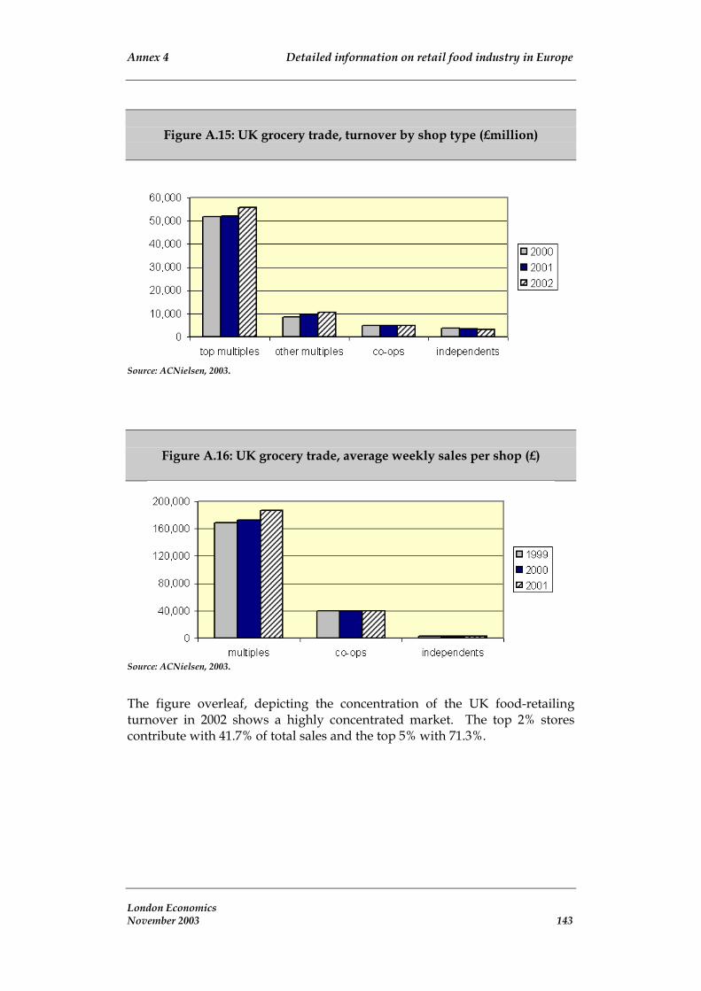
Annex 4 Detailed information on retail food industry in Europe
Figure A.15: UK grocery trade, turnover by shop type (£million)
Source: ACNielsen, 2003.
Figure A.16: UK grocery trade, average weekly sales per shop (£)
Source: ACNielsen, 2003.
The figure overleaf, depicting the concentration of the UK food-retailing turnover in 2002 shows a highly concentrated market. The top 2% stores contribute with 41.7% of total sales and the top 5% with 71.3%.
London Economics November 2003 143

Annex 4 Detailed information on retail food industry in Europe
Figure A.17: UK concentration of turnover, January 2002
Source: ACNielsen, 2003.
London Economics November 2003 144

Annex 5Empirical investigations into buying power and farm gate-retail price spreads
Annex 5 Empirical investigations into buying power and farm gate-retail price spreads
Empirical investigations into buying power and farm gate-retail price spreads
Both types of market power are in principle positively correlated with concentration. Thus, the fewer the firms in the industry, the higher profit margins, or similar performance measures, are expected to be. This is the basis for the reduced form equation estimation in the structure-conduct-performance paradigm, in which price margins, profits, market power and industrial concentration are closely related variables.
A number of approaches have been used in the economic literature on concentration, profitability and spreads. Below we provide an overview of the major methodological approaches.
First, we present the traditional structure-conduct-performance (SCP) approach that, in its empirical work, relies on reduced form models. Next we present the key features of the new empirical industrial organisation approach that relies on structural models. Another important strand of research in agricultural economics uses time series methods in a largely astructural approach.
Reduced form estimation studies based on the structure-conduct-performance paradigm Economic theory suggests that firms in a concentrated market, if protected from competition through some form of entry barriers, are expected to make supra-normal profits.
A firm with market power in the sell market is able to sell at a higher price than a corresponding firm in a competitive market because its buyers will not so easily be able to substitute away to lower price sellers. Similarly, a firm with buyer power will be able to pay less for some of its inputs than a comparable firm that needs to compete for its suppliers.
The emphasis of this approach is on a one-way causal relationship where the structural characteristics of an industry determine the conduct or behaviour of firms in that industry, which then in turn determines measures of performance such as profit rates (Bain 1951). In this paradigm, conduct is a consequence of structure and therefore does not receive much attention by this branch of the literature.
This approach tests the relationship between performance measures, such as profits, profit margins, price spreads, or simply prices, and market structure
London Economics November 2003 145

Annex 5Empirical investigations into buying power and farm gate-retail price spreads
indicators, such as concentration ratios. If this relationship is found to be statistically significant, this is taken as an indication of market power.
The approach can, in principle, capture both retail level buyer power and seller power, but distinguishing the two may not always be easy, particularly if measures of concentration in the sell and the buy markets are highly correlated, as might sometimes be the case.
Early work focused principally on cross-section studies of many industries, and whether profits were higher in more concentrated industries. Performance measures were typically accounting profit rates or price-cost margins. Structural characteristics of industries were typically 4-firm or 8-firm concentration ratios, with controls for other elements of industry structure (and conduct). Later studies added more and more control variables. Reviews of this generally cross-sector empirical work include Weiss (1971), (1974) and (1990), Vernon (1972), and Scherer (1980).
Reviews in the food sector context were undertaken by Helmberger et al. (1981) and Griffith and Gill (1984). These reviews concluded that the majority of studies showed a significant positive effect of concentration on profits or margins, and that this relationship was quite robust across different time frames, countries, measures of structure and performance, other variables, units of observation, data sets and data sources. In particular, the key conclusion regarding food retailing is that markets with small numbers of larger retail firms were more profitable than markets with a large number of smaller retail firms.
Examples of early work of this kind focusing on food retailing includes Marion et al. (1977, 1979a,b), Hall, Schmitz, and Cothern (1979), Lamm (1981), and Cotterill (1986). These studies benefit from a number of advantages relative to the broader cross-sectoral evaluations of the SCP paradigm. Because food retailing is a single industry with geographically distinct markets, both profits and product prices can be compared across the sample markets. Moreover, the underlying production technologies are broadly similar across the markets, reducing concerns about misspecification of costs, which render the SCP approach problematic in cross-industry studies.
This entire literature is nonetheless subject to the critique put forward in Demsetz (1973), that market concentration is correlated with profits because efficient (i.e., low-cost) firms acquire greater market shares over time, not because of pricing power.
Cotterill (1993) subsequently suggested that, while efficiencies might explain profit variations they cannot justify price variations. A more recent version of the Demsetz critique is that food retailing is essentially a joint product, bundling items for sale with a potentially wide range of services. Since the provision of services is costly, a positive correlation between price and concentration may simply reflect the fact that firms in concentrated markets and with higher market shares offer more services, charging higher prices to cover the costs.
London Economics November 2003 146

Annex 5Empirical investigations into buying power and farm gate-retail price spreads
Studies that do not control for variations in service levels may find that market concentration causes higher prices, but these findings may be spurious. However, this critique applies to results based on price differences across food retailers, but cannot explain the positive relationship between structure and profits, as noted above.
Although some studies have investigated whether rates of return are higher in large firms because of greater efficiency rather than collusive conduct or abuse of market power, a general criticism of this branch of research is that the evidence that higher concentration causes higher profits provides no information about the source of the increased profits, i.e. says nothing about the behaviour of the firms making up the industry and whether they exert some sort of market power or are just more efficient. This criticism led to a renewed interest in firm conduct and the development of the New Empirical Industrial Organisation.
New Empirical Industrial Organisation structural estimation Dissatisfaction with the identification problems arising from reduced-form equations has lead to a number of studies explicitly designed to exploit the structure of oligopoly models. The focus of the New Empirical Industrial Organisation (NEIO) literature is thus on the conduct of firms within a particular industry. NEIO models specify the first-order conditions for the profit maximizing behaviour of a single oligopolist.
A key behavioural parameter in this approach is the conjectural variation of the oligopolist, which measures the degree to which a firm takes into account its rivals’ reactions to its own output choice. Conjectural variations (CV) models assume that firms base output decisions on the response they expect to get from competitors.
The expectation of a limited market response to a change in firm output suggests that the market is competitive, while the expectation of an extensive market response suggests the presence of market power.
Tests using the CV framework explicitly permit the decision process of a single firm to be affected by the behavior of rival firms. Assuming the model accurately describes underlying conditions, this allows direct predictions of firm beliefs (conjectures) regarding rival actions, and therefore of firm behavior. The CV model does not require that the conjectures be specified ex ante, but instead uses empirical data to provide information about the nature of the conjectures.
A typical CV model uses the single firm’s profit maximization condition to derive a profit maximizing output response condition. The output response depends on the price elasticity of input supply and output demand, and on the firm’s “conjecture” about industry response to a change in its own production level. The response function is modeled such that a single parameter, the conjectural elasticity, measures the difference between the
London Economics November 2003 147

Annex 5Empirical investigations into buying power and farm gate-retail price spreads
input price and the firm’s marginal valuation of output (called the price-cost margin, or Lerner index).
Data on input and output prices and marginal cost are used to estimate the conjectural elasticity, and thus determine whether market power (power to raise price above marginal costs) exists.
The CV parameter can vary continuously between values implying perfectly competitive behaviour or pure collusion. Thus an econometric model can specify simultaneously the first-order condition of the firm, the market equilibrium condition, a market demand function, and an endogenous relationship for the conjectural variation variable, with cross-equation restrictions imposed. Under rather restrictive conditions, the model can be econometrically identified and an estimate for the conjectural variation parameter can be obtained.
From this, one can infer the degree of oligopoly power in the market. More complicated versions of the model allow for vertical oligopoly interaction between food manufacturers and supermarkets.
The NEIO literature up to the late 1980s has been surveyed by Geroski (1988) and Bresnahan (1989). Wohlgenant (1999) provides an updated review of the various models researchers have used to examine food marketing margin behaviour, including the behaviour of non-competitive components of the marketing chain.
Despite the attractiveness of a detailed structural model, the application of NEIO methods to food retailing has a number of drawbacks.
A major shortcoming of this methodology is the fact that it relies crucially on accurate estimates of the underlying market and technological conditions. In order to obtain estimates of firm conjectures, the researcher must provide estimates of the price elasticity of demand, and/or the wage elasticity of supply, or estimate them concurrently with firm conjectures.
Moreover, correct specification of output demand, input supply and production costs is necessary for estimates of market power to be accurate. If any of the estimated supply/demand or cost functions is incorrect, conclusions regarding firm conjectures may also be incorrect.
An important problem is also that, due to a frequent lack of firm-level data, market level data are in practice most often used in the estimation35. The underlying theoretical model does not directly support this type of specification since it relies on the individual firm’s optimality conditions. The estimates resulting from an industry-wide estimation of conjectural variations are thus loosely interpreted as an empirical index of market power.
35 Often, the assumption is made that all firms are identical and that, therefore, one can undertake the empirical estimation of the model at the industry level.
London Economics November 2003 148

Annex 5Empirical investigations into buying power and farm gate-retail price spreads
Finally, the NEIO models raise a number of econometric identification problems. Proper identification may require at least one statistically significant interaction term between the output price variable and an exogenous variable in the demand function in order to include changes in the slope of the demand as well as shifts in demand over the estimation period.36
O’Donnell (1999) uses this sort of approach in the context of a marketing margin model. He takes a general industry model, imposes restrictions consistent with some specific assumptions about fixed proportions, linear demand, normalised quadratic costs, and constant returns to scale, and generates an estimating equation for the farm-retail margin. Coefficients on the quantity variables in the models are functions of the conjectural variations parameters in input and output markets. A test of whether these coefficients are significantly different from zero is equivalent to a test of whether the conjectural variations are significantly different from zero. If they are, market power is implied; if they are not competitive behaviour is implied.
In the most recent and most rigorous treatments for the food industry, Muth and Wohlgenant (1999b), for food manufacturing, and Park and Weliwita (1999), for food retailing, use a two-equation model based on Bresnahan (1989) which includes the demand function facing the industry and the industry equilibrium condition where marginal cost equals perceived marginal revenue.
This latter equation includes a parameter that is an index of market power, and this is can be allowed to vary in response to changes in industry conditions and technical innovations. Thus the degree of market power is estimated from actual data. The results are found to depend on whether the market power terms are held fixed or are allowed to vary with changing industry conditions.
Park and Weliwita conclude that, in the US, food retailers act like price takers. Schroeter, Azzam, and Zhang (2000) is another attempt to test for retailer market power, but explicitly in the context of vertical competition between food retailers and food manufacturers. The model allows for the estimation of the seller power of manufacturers, and both the seller and buyer power of retailers. Thus, there are three conjectural variations parameters to be estimated in all, making this study more complicated than the previous one.
The main point of the study is to test a series of hypotheses on market power in the wholesale market: bilateral price-taking, retailer price-taking, and manufacturer price-taking. The possibility of vertically collusive behaviour in the wholesale market is not tested. The endogenously determined food retail seller power is simultaneously estimated in each case.
The authors find that the hypothesis of bilateral price-taking in the wholesale market is rejected in a pair-wise comparison with retail price-taking, but not
36 In essence, these models require that the demand elasticity varies over the sample period so that all parameters of interest can be identified.
London Economics November 2003 149

Annex 5Empirical investigations into buying power and farm gate-retail price spreads
in a comparison with manufacturer price-taking. Furthermore, a non-nested test rejects retail price-taking in favour of manufacturer price-taking.
These results lead the authors to conclude that food retailers enjoy market power in the wholesale market, but manufacturers do not. Thus this study provides some evidence in favour of the sentiment that supermarkets have acquired buying power in the wholesale market.
In a series of influential papers, Paul (1999 a,b,c) stressed the need for a rigorous treatment of the cost structure of the industry when attempting to measure market power effects.
The bottom line is that the NEIO approach, while theoretically highly appealing, is very complex in applying empirically and often requires the researcher to make simplifying assumptions that, if not valid, can seriously undermine the robustness of the empirical results.
Time series methods Another recent strand of research examines the time series properties of the major price series in a particular food chain to infer industry behaviour from market outcomes.
For example, Reed and Clark (1998) used cointegration methods on data from seven US food industries. These data contained both deterministic and stochastic trends, and the authors focus on the effects of different ways of handling these trends.
They found that ignoring the stochastic trends leads to a rejection of the competitive model hypothesis for six of the seven industries (like Azzam and Pagoulatus 1990); that removing these trends by differencing leads to a rejection of the competitive model hypothesis for none of the seven industries (like Wohlgenant 1989); and that properly accounting for them leads to a rejection of the competitive model hypothesis for only two of the seven industries.
Thus analysts are more likely to reject competitive market behaviour if they do not correctly account for the characteristics of the data series they are using. These authors also make the point that “... deciding whether markets are competitive rests not on whether an industry establishes a gap between price and marginal cost but on whether the gap is maintained over time and as capital moves in and out of the sector”.
Goodwin and Holt (1999) also used cointegration methods to examine the long-run equilibrium relationships between US farm, wholesale and retail beef prices, with a particular emphasis on the causal direction of price changes and on whether responses were symmetric to price rises and price falls. They found unidirectional price transmission, from farm to wholesale to retail, which does not imply the existence of market power at higher levels of the chain.
London Economics November 2003 150

Annex 5Empirical investigations into buying power and farm gate-retail price spreads
They also found that the responsiveness to price shocks had increased in recent years and they suggested that this result may imply that markets have become relatively more efficient in transmitting information through vertical marketing channels.
Palaskas (1995) used cointegration methods to examine the dynamic transmission of five agricultural producer prices through the food marketing system in seven countries of the European Union. Statistical tests rejected the hypothesis of perfect short-run price transmission across all pairs of prices in all countries. Furthermore, in the long run, perfect price transmission was not rejected in only two of five price pairings across six of the countries. The UK was the exception. So for all products in the UK and for three of the products in the other six countries, non-competitive behaviour was concluded.
Dawson and Tiffen (1997) also use cointegration models to examine beef, lamb and pork farm and retail prices in the UK. They did not find a cointegrating relationship for either beef or pork and while they did find one for lamb, the relationship implied causality from retail to producer prices. This suggests that for the lamb industry, prices are set at the retail level and thus there is some evidence of market power in retailing, while for the beef and pork industries there is some evidence against a competitive market.
In the case of studies of European food chains, the most widely used methodology is that of time series analysis focusing on price transmission, between the upstream and downstream ends of the supply chain.
London Economics November 2003 151

Annex 6 Detailed estimation results of asymmetric price transmission models
Annex 6 Detailed estimation results of asymmetric price transmission models
Methodology for testing for asymmetric price transmission
Introduction The standard approach to test for price transmission is based on the asymmetric error correction model proposed by Engle and Granger (1987).
For any country and sector, let PDt and PUt be the logarithms of the downstream (D) and upstream (U) price, respectively, in the vertical supply chain at time t. The methodology involves the following five steps.
Step 1: Estimating the long-run relationship between downstream and upstream prices As a first step we will test whether each of the time series is integrated of order one, i.e. first differences of the data ensures stationarity. We will use the augmented Dickey-Fuller (ADF) test to test for stationarity. In addition, the Kwiatkowski et al. (1992) test (or KPSS test) can be implemented to ensure that the series are first difference stationary, in other words, if they are I(1).
If the series are found to be integrated of order one, we will then proceed to estimate the long-run equilibrium relationship between downstream and upstream as:
PDt = α10 + α11 PUt + u1t ,
where PDt and PUt are the prices at different levels of the supply chain (as defined above), α10 and α11 are parameters to be estimated, and u1t is an error term. Equivalently, an equation can be estimated for the long-run relationship between upstream and downstream: PUt = α20 + α21 PDt + u2t with the variables defined as above.
If the estimated residuals û1t are stationary, then PDt and PUt are cointegrated and there exists an error correction representation (Engle and Granger, 1987). Test statistics and tables provided by Engle and Granger (1995) will be used to test the hypothesis of stationarity of the residuals (similarly for û2t).
When the price series are cointegrated, the short-run dynamics can be represented using an error-correction model that includes an error correction term (ECT) that accounts for deviations from the cointegrating relation between PDt and PUt:
∆PDt = β0 + β1 ECT1t-1 + β2(L)∆PDt-1 + β3(L)∆PUt-1 + εt London Economics November 2003 152

Annex 6 Detailed estimation results of asymmetric price transmission models
∆PUt = γ0 + γ 1 ECT2t-1 + γ 2(L)∆PUt-1 + γ3(L)∆PDt-1 + νt ,
where ECT2t-1 = û1t-1 and ECT2t-1 = û2t-1, βk(L) and γk(L) are lag polynomials and εt and νt are error terms. Lag lengths are chosen using AIC criterion and such that residuals are serially uncorrelated.
Step 2: Accounting for asymmetric adjustment The threshold autoregressive (TAR) model allows a segmentation of the error correction term into positive and negative components. When the price series are shown to be cointegrated by an asymmetric adjustment, the short-run dynamics can be represented using an error-correction model of the form:
∆PDt = β0 + β+1 ECT+1t-1 + β-1 ECT-1t-1 + β2(L)∆PDt-1 + β3(L)∆PUt-1 + εt
∆PUt = γ0 + γ+1 ECT+2t-1 + γ-1 ECT-2t-1 + γ2(L)∆PUt-1 + γ3(L)∆PDt-1 + νt ,
where the error correction terms ECT+1t-1 = û+1t-1 and ECT-1t-1 = û –1t-1 are defined as û +1t+1 = û 1t+1 if û 1t+1 > 0 and 0 otherwise, and û -1t-1 = û 1t-1 if û 1t-1 < 0 and 0 otherwise from the long-run equilibrium relationship (similarly for defining ECT+2t-1 = û+2t-1 and ECT-2t-1 = û –2t-1).
An F-test can be used to test whether β+2 = β-2, and hence test whether price transmission between PDt and PUt is symmetric (the same can be done for testing symmetric transmission between PUt and PDt).
Inclusion of other relevant effects The BSE crisis led to a decline in beef consumption and an increase in the demand for other meats. The possibility that the BSE crisis may have caused a structural break in the cointegrating equation in the first half of 1996 will also be considered37. Similarly, we will need to assess the potential impact of foot and mouth disease on the farm-retail price spreads of beef and lamb.
For each of the selected products, potential structural breaks will be identified through simple chart analysis and identification of major events that could have changed the underlying relationship between upstream and downstream prices.
London Economics November 2003 153
37 As Von Cramon-Taubadel and Meyer (2000) show, the presence of structural breaks in the observed
relationship between an upstream and a downstream price in the supply chain can lead to too frequent a rejection of the hypothesis that the transmission of price shocks is symmetric and biases the conclusions of the empirical analysis in favour of asymmetric price transmission.
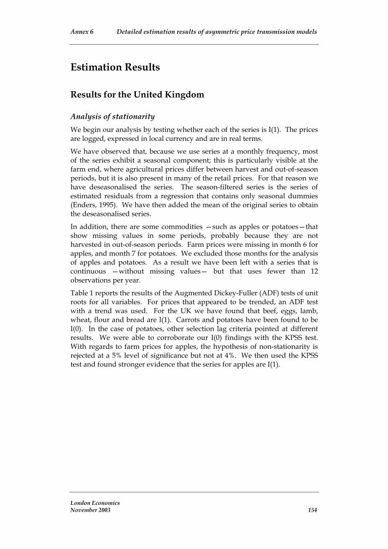
Annex 6 Detailed estimation results of asymmetric price transmission models
Estimation Results
Results for the United Kingdom
Analysis of stationarity We begin our analysis by testing whether each of the series is I(1). The prices are logged, expressed in local currency and are in real terms.
We have observed that, because we use series at a monthly frequency, most of the series exhibit a seasonal component; this is particularly visible at the farm end, where agricultural prices differ between harvest and out-of-season periods, but it is also present in many of the retail prices. For that reason we have deseasonalised the series. The season-filtered series is the series of estimated residuals from a regression that contains only seasonal dummies (Enders, 1995). We have then added the mean of the original series to obtain the deseasonalised series.
In addition, there are some commodities —such as apples or potatoes—that show missing values in some periods, probably because they are not harvested in out-of-season periods. Farm prices were missing in month 6 for apples, and month 7 for potatoes. We excluded those months for the analysis of apples and potatoes. As a result we have been left with a series that is continuous —without missing values— but that uses fewer than 12 observations per year.
Table 1 reports the results of the Augmented Dickey-Fuller (ADF) tests of unit roots for all variables. For prices that appeared to be trended, an ADF test with a trend was used. For the UK we have found that beef, eggs, lamb, wheat, flour and bread are I(1). Carrots and potatoes have been found to be I(0). In the case of potatoes, other selection lag criteria pointed at different results. We were able to corroborate our I(0) findings with the KPSS test. With regards to farm prices for apples, the hypothesis of non-stationarity is rejected at a 5% level of significance but not at 4%. We then used the KPSS test and found stronger evidence that the series for apples are I(1).
London Economics November 2003 154

Annex 6 Detailed estimation results of asymmetric price transmission models
Table A.30: Results of ADF test
PP RP
Original Series
First Difference
Original Series
First Difference
Beef -0.68 (2) -9.21* (2) -0.04 (0)
-3.70* (0) -- -3.70* (0) --
Potatoes -4.98* (9) -- -3.62t* (5) --
-7.35* (5) -2.81 (0) -12.33*(0)
Eggs -1.16 (3) -6.24* (2) -3.13t (1) -18.51t* (0)
Lamb -2.29 (12) -3.70* (12) -1.77 (12) -4.74* (12)
Wheat/Bread -0.91 (1) -15.27* (0) -1.54 (0) -14.80* (0)
Wheat/Flour -0.91 (1) -15.27* (0) -1.13 (0)
-13.29* (0)
Carrots
Apples -3.00* (1)
-14.57* (0)
Lag length selected on the basis of the AIC, except for † where SBC and HQC criteria are used.
PP producer prices, RP retail prices
Cointegration: estimation of a long-run relationship
• The deseasonalised series for the eggs and the wheat/flour long-run relationship shows non-stationarity of the residuals under different specifications.
• The deseasonalised series for apples and the wheat/bread long-run relationship shows stationarity of the residuals. The deseasonalised series for potatoes shows stationary residuals in the long-run relationship when a trend is included.
t denotes ADF test with a trend. * Rejection of the null hypothesis of non-stationarity
We have tried several long-run specifications for each of the selected products. In the case of apples and carrots in the UK we use only 11 monthly observations. The estimation results for the retail-producer long-run relationship (equation 1) are presented in Table 2:
• The deseasonalised series for beef showed non-stationarity of the residuals in the long-run relationship. However, after inclusion of two dummy variables to account for the BSE breaks, we found stationary residuals in the long-run relationship for both the consumer and farm prices. A first dummy (D1989m7) takes into account the announcement (28/07/89) of the EC ban on export of cattle born before 18/07/88 and of offspring of affected or suspected animals. Hence, a dummy variable is constructed that takes value 1 after July 1989, and 0 otherwise. And a second dummy variable (D1996m3) accounts for the Commission Decision 96/239/EC that prohibited the export from the UK of live bovine animals, their semen and embryos;
London Economics November 2003 155

Annex 6 Detailed estimation results of asymmetric price transmission models
meat of bovine animals slaughtered in the UK. This variable takes value of 1 after March 1996, 0 otherwise38.
• The deseasonalised series for lamb showed contradictory results. In the first specification tried there was evidence of non-stationarity of the residuals. In an additional specification we included dummies allowing for the BSE structural breaks used in the analysis of beef. When testing for stationarity by using a lag structure on the basis of AIC criterion (12 lags) the null hypothesis of non-stationarity could not be rejected. However, for other lag structures chosen on the basis of the Schwartz-Bayesian and Hannan-Quinn criteria (both indicating 0 lags as optimal) the null hypothesis was widely rejected (ADF of -6.03). Moreover, we also observed that for other lag structures (from 0 to up to 5 lags) the statistic was also rejecting non-stationarity. In addition, we observed that for a restricted sample period (from 1986m1 to 2002m6) all three criteria could reject the hypothesis of non-stationarity. For these reasons we concluded that it is likely that a cointegration relationship exists between the two lamb prices, once the dummies for BSE are included.
38 Source http://www.defra.gov.uk/animalh/bse/chronol.pdf.
London Economics November 2003 156

Annex 6 Detailed estimation results of asymmetric price transmission models
Table A.31: Retail-producer long-run equations.
Chain analysed Long-run equation Sample period
ADF1 test for
stationarity of û1t (lags)
Wheat/bread(d) PRt =0.60+0.42PPt + u1t -3.9* (0) 1987m1-2001m12
PRt =-0.03+0.36PPt + u1t -2.84 (0) 1987m1-2001m12
Beef(d) PRt = 0.96+0.53PPt+0.05D1989m7+0.05D1996m3 + u1t -5.04* (1) 1986m1-2003m6
Lamb(d) PRt = 1.16+0.29PPt+0.03D1989m7+0.12D1996m3 + u1t -6.03†* (0) 1986m1-2003m6
Apples(d) PRt = 0.46+0.46PPt + u1t -4.00* (12) 1987m1-2000m12
Potatoes(d) PRt = -0.12+0.0TREND+0.43PPt + u1t -4.57* (0) 1987m1-2001m12
Carrots(d) PRt = 0.35-0.00TREND+0.36PPt + u1t -5.76* (0) 1987m1-2001m12
Eggs(d) PRt = 0.45-0.02PPt + u1t -2.48 (1) 1992m1-2003m3
Wheat/flour(d)
1 Model chosen on the basis of AIC criterion except for † where SBC and HQC where used. 2 Deseasonalised series are indicated by (d). * Residuals stationary (rejection of null hypothesis of non-stationarity at 95% level).
The results for the producer-retail long-run relationship are presented in Table A.32, and show similar cointegration results than the previous table. One exception is the equation for apples, where a trend was needed to make the residuals stationary.
London Economics November 2003 157

Annex 6 Detailed estimation results of asymmetric price transmission models
Table A.32: Producer-retail long-run equations.
Chain analysed Long-run equation ADF1 test for
stationarity of û1t (lags)
Sample period
Wheat/bread(d) PPt =-1.50+2.17PRt + u2t -3.9* (0) 1987m1-2001m12
Wheat/flour(d) PPt =-0.34+2.23PRt + u2t -2.8 (0) 1987m1-2001m12
Beef(d) PPt =-1.21+1.50PRt -0.11D1989m7 – 0.17D1996m3+ u2t -6.23* (1) 1986m1-2003m6
Lamb(d) PPt =-1.84+2.00PRt -0.15D1989m7 – 0.29D1996m3+ u2t -5.61*† (0) 1986m1-2003m6
Apples(d) PPt =-0.62+0.87PRt –0.00TREND + u2t -6.30* (12) 1987m1-2000m12
Potatoes(d) PPt =-0.28+1.78PRt –0.01TREND + u2t -4.23* (0) 1987m1-2001m12
PPt =-1.18+0.80PRt + u2t -3.67* (0) 1987m1-2001m12
Eggs(d) PPt =-0.77+0.50PRt + u2t -2.04 (7) 1992m1-2003m3
Carrots(d)
1 Model chosen on the basis of AIC criterion except for † where SBC and HQC where used. 2 Deseasonalised series are indicated by (d). * Residuals stationary (rejection of null hypothesis of non-stationarity at 95% level).
In the next sections we present the results of the error correction models for retail and producer models. For purposes of comparison, estimates of both asymmetric and symmetric error correction models are presented, for the models for retail prices and for the producer prices. The models include the Breusch-Godfrey LM statistic, with different lags, for testing autocorrelated residuals.
Apples The t-statistics for ECTt-1 in the column for retail price indicate that retail prices respond to shocks that make the relationship deviate from the long-run equilibrium. The symmetry test cannot be rejected.
The result for the equation of farm prices is the following: there is a long-run relationship (evidence of transmission) but when allowing for asymmetric transmission we observe that ECT+t-1 and ECT-t-1 are individually significant at 5% but we cannot reject the hypothesis that the parameters are equal.
The Granger-causality tests suggest that transmission is bi-directional, in the sense that farm prices are affecting consumer prices but consumer prices are also affecting farm prices. London Economics November 2003 158

Annex 6 Detailed estimation results of asymmetric price transmission models
Estimates of the Error correction models for Apples (retail prices) ∆RP APPLES Symmetric Asymmetric
∆PP 0.15 (4.77)** 0.15 (4.66)**
∆PPt-1 0.12 (3.78)** 0.13 (3.80)**
ECTt-1 -0.21 (4.18)** --
ECT+t-1 -- -0.24 (3.06)**
ECT-t-1 -- -0.16 (1.71)+
Constant -0.00 (0.10) 0.00 (0.32)
Observations 163 163
R-squared 0.25 0.25
17.32 [0.00] 12.99 [0.00]
Symmetry Test 0.25 [0.62]
Q(1) 0.01 [0.91] 0.02 [0.88]
1.93 [0.38] 1.95 [0.37]
Q(12) 10.86 [0.54]
Test Granger
Q(2)
10.59 [0.56]
Absolute value of t statistics in parentheses. + significant at 10%; * significant at 5%; ** significant at 1%.
Q(T) denote the Breusch-Godfrey LM statistic for testing autocorrelated residuals with T lags. P-value in square brackets.
Estimates of the Error correction models for Apples (producer prices) Symmetric Asymmetric
∆PPt-1 -0.18 (2.23)* -0.18 (2.24)*
∆RP 0.82 (5.28)** 0.83 (5.26)**
∆RPt-1 0.04 (0.29) 0.05 (0.32)
∆RPt-2 0.22 (1.45) 0.22 (1.45)
EMTt-1 -0.58 (6.32)** --
-- -0.54 (3.31)**
ECT-t-1 --
0.00 (0.09) -0.00 (0.20)
Observations 162 162
R-squared 0.39 0.39
Test Granger 15.96 [0.00] 12.71 [0.00]
Symmetry Test 0.10 [0.76]
Q(1) 0.70 [0.40] 0.02 [0.88]
0.90 [0.63] 1.95 [0.37]
Q(12) 6.02 [0.91]
∆PP APPLES
ECT+t-1
-0.61 (4.18)**
Constant
Q(2)
10.59 [0.56]
Absolute value of t statistics in parentheses. + significant at 10%; * significant at 5%; ** significant at 1%. Q(T) denote the Breusch-Godfrey LM statistic for testing autocorrelated residuals with T lags. P-value in square brackets.
London Economics November 2003 159

Annex 6 Detailed estimation results of asymmetric price transmission models
Carrots The series for retail and producer prices are I(0) after deseasonalisation. We have therefore estimated an error correction model in levels.
In the equation for consumer prices we are using one lag for the dependent retarded variable and one lag for the farm prices (in addition to the contemporaneous farm prices). The t-statistic for ECTt-1 indicate that retail prices are cointegrated with producer prices, responding to shocks that make the relationship deviate from the long-run equilibrium. Asymmetric adjustment in the retail price model cannot be concluded, because the F test for equality of both parameters cannot be rejected (F value is 0.57 with a p-value of 0.45).
The equation of farm prices is estimated using the contemporaneous consumer prices with two additional lags. The results are the same than for retail price: farm prices are cointegrated with retail prices, responding to shocks that make the relationship deviate from the long-run equilibrium. However, such adjustment is symmetric because the F test for equality of both parameters cannot be rejected (F value is 0.05 with a p-value of 0.82).
Granger-causality tests suggest that causality runs symmetrically in both directions. Farm prices are affecting consumer prices, and are also being affected by consumer prices.
Estimates of the Error correction models for Carrots (retail prices) RP CARROTS Symmetric Asymmetric
RPt-1 1.00 (24.67)** 1.00 (24.26)**
PPt 0.28 (7.19)** 0.28 (7.19)**
PPt-1 -0.26 (6.14)** -0.26 (6.18)**
(4.93)**
ECT+t-1 -0.28 (2.70)**
ECT-t-1 -0.42 (3.39)**
0.03 (0.85) 0.02 (0.61)
Observations 179 179
R-squared 0.88 0.88
27.15 20.45
Test Granger 27.15 [0.00] 20.45 [0.00]
Q1 0.50 [0.48] 0.55 [0.46]
1.65 [0.44] 1.96 [0.38]
Q12 6.11 [0.91] 6.33 [0.90]
Symmetry test 0.57 [0.45]
ECTt-1 -0.34
Constant
Test Granger
Q2
Absolute value of t statistics in parentheses. + significant at 10%; * significant at 5%; ** significant at 1%. Q(T) denote the Breusch-Godfrey LM statistic for testing autocorrelated residuals with T lags. P-value in square brackets.
Estimates of the Error correction models for Carrots (producer prices)
London Economics November 2003 160

Annex 6 Detailed estimation results of asymmetric price transmission models
PP CARROTS Symmetric Asymmetric
0.77 (7.38)** 0.77 (7.35)**
RPt-1 0.13 (0.93) 0.13 (0.94)
RPt-2 -0.14 (1.33) -0.14 (1.32)
(20.76)**
ECT+t-1 0.85 (11.56)**
ECT-t-1 0.82 (10.28)**
-1.19 (47.80)** -1.20 (45.44)**
Observations 178 178
R-squared 0.82 0.82
195.15 [0.00] 155.27 [0.00]
Q1 0.34 [0.56] 0.39 [0.53]
Q2 0.27 [0.87] 0.32 [0.85]
Q12 11.23 [0.51] 11.21 [0.51]
Symmetry test 0.05 [0.82]
RPt
ECTt-1 0.84
Constant
Test Granger
Absolute value of t statistics in parentheses. + significant at 10%; * significant at 5%; ** significant at 1%. Q(T) denote the Breusch-Godfrey LM statistic for testing autocorrelated residuals with T lags. P-value in square brackets.
Potatoes The t-statistics for ECTt-1 in the column for retail price indicate that retail prices respond to shocks that make the relationship deviate from the long-run equilibrium. Retail prices asymmetric adjustment is rejected because the F test for equality of both parameters cannot be rejected (F value is 1.35 with a p-value of 0.25).
The equation of farm prices requires of a high number of lags to achieve non-autocorrelated residuals. The symmetry test shows that we cannot reject the hypothesis of symmetric adjustment.
Finally, the Granger-causality tests suggest that transmission is bi-directional, in the sense that farm prices are affecting consumer prices but farm prices are also being affected by consumer prices.
London Economics November 2003 161
Estimates of the Error correction models for Potatoes (retail prices) RP POTATOES Symmetric Asymmetric
RPt-1 1.01 (41.07)** 1.02 (40.96)**
PPt 0.32 (8.54)** 0.32 (8.60)**
PPt-1 -0.30 (8.00)** -0.31 (8.04)**
ECTt-1 -0.28 (4.95)**
ECT+t-1 -0.20 (2.32)*
ECT-t-1 -0.40 (3.46)**
Constant 0.04 (1.67)+ 0.04 (1.58)
Observations 158 158
R-squared 0.95 0.95

Annex 6 Detailed estimation results of asymmetric price transmission models
Test Granger 40.46 [0.00] 30.75 [0.00]
Q1 0.07 [0.79] 0.17 [0.68]
Q2 0.74 [0.69] 0.67 [0.71]
Q12 9.12 [0.69] 9.27 [0.69]
Symmetry test 1.35 [0.25]
Estimates of the Error correction models for Potatoes (producer prices) PP POTATOES Symmetric Asymmetric
PPt-1 0.95 (12.40)** 0.97 (12.47)**
PPt-2 0.05 (0.50) 0.03 (0.35)
PPt-3 -0.04 (0.44) -0.02 (0.22)
PPt-4 0.01 (0.11) 0.00 (0.03)
PPt-5 -0.05 (0.58) -0.05 (0.55)
PPt-6 0.05 (0.50) 0.03 (0.34)
PPt-7 0.04 (0.46) 0.04 (0.44)
PPt-8 0.16 (1.76)+ 0.16 (1.81)+
PPt-9 -0.10 (1.05) -0.09 (0.99)
PPt-10 -0.18 (2.62)** -0.18 (2.66)**
RPt 0.94 (7.97)** 0.94 (7.96)**
RPt-1 -0.99 (7.95)** -1.00 (8.04)**
ECTt-1 -0.12 (1.91)+
ECT+t-1 -0.25 (2.13)*
ECT-t-1 -0.05 (0.70)
Constant -0.27 (4.28)** -0.24 (3.51)**
Observations 149 149
R-squared 0.94 0.95
Test Granger 22.43 [0.00] 17.36 [0.00]
Q1 0.05 [0.82] 0.28 [0.60]
Q2 0.49 [0.78] 1.24 [0.54]
Q12 16.73 [0.16] 18.19 [0.11]
Symmetry test 1.77 [0.19]
Absolute value of t statistics in parentheses. + significant at 10%; * significant at 5%; ** significant at 1%. Q(T) denote the Breusch-Godfrey LM statistic for testing autocorrelated residuals with T lags. P-value in square brackets.
Beef In the equation for beef prices we selected the optimal lag structure with the AIC criterion. Our chosen model for retail prices uses only the contemporaneous farm price, in addition to the lagged error correction term. We experimented including the dummy variables for the BSE breaks but they were not statistically significant in the ECM equation (although they are present in the long-run relationship).
London Economics November 2003 162

Annex 6 Detailed estimation results of asymmetric price transmission models
The retail price appears to be cointegrated with producer prices, hence, retail prices react to shocks that make the retail-producer relationship deviate from the long-run equilibrium. When allowing for asymmetric transmission we observe that we cannot reject symmetric price transmission.
The result for the farm prices equation is the following: there is evidence of transmission (the absolute t-statistic for ECTt-1 is 5.51) but we cannot reject that the transmission is symmetric (F test equals 0.01, with p-value of 0.9).
Finally, the Granger-causality tests suggest that transmission is bi-directional, in the sense that farm prices are affecting consumer prices but consumer prices are also affecting farm prices.
Estimates of the Error correction models for Beef (retail prices) ∆RP BEEF Symmetric Asymmetric
∆PP 0.21 (7.85)** 0.21 (7.74)**
ECTt-1 -0.16 (4.68)** --
-- -0.09 (1.45)
ECT-t-1 -- -0.24 (3.43)**
Constant -0.00 (0.92) -0.00 (1.58)
Observations 209 209
R-squared 0.28 0.28
Test Granger 39.56 [0.00] 27.00 [0.00]
Symmetry test 1.65 [0.20]
Q1 0.03 [0.85] 0.10 [0.76]
Q2 0.22 [0.90] 0.27 [0.87]
Q12 13.06 [0.36] 13.77 [0.32]
ECT+t-1
Absolute value of t statistics in parentheses. + significant at 10%; * significant at 5%; ** significant at 1%. Q(T) denote the Breusch-Godfrey LM statistic for testing autocorrelated residuals with T lags. P-value in square brackets.
Estimates of the Error correction models for Beef (producer prices) ∆PP BEEF Symmetric Asymmetric
∆PPt-1 0.33 (4.59)** 0.33 (4.57)**
∆RP 0.91 (7.04)** 0.91 (7.02)**
∆RPt-1 -0.24 (1.67)+ -0.23 (1.65)
∆RPt-2 0.01 (0.07) 0.01 (0.07)
∆RPt-3 0.01 (0.08) 0.01 (0.09)
0.18 (1.43) 0.18 (1.43)
∆RPt-5 -0.07 (0.54) -0.07 (0.54)
∆RPt-6 0.08 (0.63) 0.08 (0.64)
∆RPt-7 -0.41 (3.35)** -0.41 (3.29)**
∆RPt-8 0.15 (1.20) 0.15 (1.18)
∆RPt-4
London Economics November 2003 163

Annex 6 Detailed estimation results of asymmetric price transmission models
ECTt-1 -0.24 (5.51)**
ECT+t-1 -0.25 (2.99)**
ECT-t-1 -0.23 (2.89)**
Constant -0.00 (0.86) -0.00 (0.43)
Observations 201 201
R-squared 0.39 0.39
Test Granger 9.47 [0.00] 8.56 [0.00]
Symmetry test 0.01 [0.91]
Q1 2.11 [0.15] 2.09 [0.15]
Q2 2.23 [0.33] 2.20 [0.33]
Q12 5.65 [0.93] 5.61 [0.93]
Absolute value of t statistics in parentheses. + significant at 10%; * significant at 5%; ** significant at 1%. Q(T) denote the Breusch-Godfrey LM statistic for testing autocorrelated residuals with T lags. P-value in square brackets.
Lamb The lag structure for the lamb equations was selected using the AIC criterion. We experimented including the dummy variables for the BSE breaks but they were not statistically significant in the ECM equation (although they are present in the long-run relationship).
The t-statistic for the ECTt-1 indicates that the retail price react to shocks that make the retail-producer relationship deviate from the long-run equilibrium. There seems to be evidence of asymmetric as the symmetry test is rejected (F test is 4.62 with a p-value of 0.03).
The result for the farm prices equation is the following. There is evidence of transmission (the absolute t-statistic for ECTt-1 is 2.52) but there is no evidence that the transmission is asymmetric.
Finally, the Granger-causality tests suggest that transmission is bi-directional, in the sense that farm prices are affecting consumer prices but consumer prices are also affecting farm prices.
Estimates of the Error correction models for Lamb (retail prices) ∆RP LAMB Symmetric Asymmetric
∆PP 0.11 (6.01)** 0.11 (5.51)**
∆PPt-1 0.18 (8.66)** 0.17 (8.49)**
∆PPt-2 0.07 (3.79)** 0.07 (3.79)**
∆PPt-3 0.03 (1.51) 0.03 (1.47)
∆PPt-4 0.02 (1.35) 0.02 (1.32)
∆PPt-5 0.04 (2.11)* 0.04 (2.19)*
∆PPt-6 0.03 (1.54) 0.02 (1.21)
ECMt-1 -0.20 (4.85)**
London Economics November 2003 164

Annex 6 Detailed estimation results of asymmetric price transmission models
ECM+t-1 -0.08 (1.22)
ECM-t-1 -0.32 (4.63)**
Constant 0.00 (0.51) -0.00 (1.38)
Observations 203 203
R-squared 0.60 0.61
Test Granger 37.06 [0.00] 34.07 [0.00]
Symmetry test 4.62 [0.03]
Q1 1.81 [0.18] 2.14 [0.14]
Q2 1.80 [0.41] 2.13 [0.35]
Q12 7.89 [0.79] 8.38 [0.75]
Absolute value of t statistics in parentheses. + significant at 10%; * significant at 5%; ** significant at 1%. Q(T) denote the Breusch-Godfrey LM statistic for testing autocorrelated residuals with T lags. P-value in square brackets.
Estimates of the Error correction models for Lamb (producer prices) ∆PP LAMB Symmetric Asymmetric
∆PPt-1 -0.12 (1.41) -0.12 (1.36)
∆PPt-2 -0.24 (3.67)** -0.24 (3.61)**
∆PPt-3 -0.19 (2.91)** -0.19 (2.87)**
∆PPt-4 -0.06 (0.92) -0.06 (0.96)
∆PPt-5 -0.10 (1.41) -0.09 (1.39)
∆PPt-6 -0.21 (3.10)** -0.21 (3.10)**
∆PPt-7 0.10 (1.52) 0.10 (1.42)
∆PPt-8 0.01 (0.08) 0.00 (0.04)
∆PPt-9 0.06 (0.95) 0.06 (0.93)
∆PPt-10 0.10 (1.55) 0.10 (1.51)
0.12 (1.83)+ 0.12 (1.87)+
∆PPt-12 0.21 (3.36)** 0.22 (3.42)**
∆RP 1.42 (6.65)** 1.39 (6.49)**
ECTt-1 -0.14 (2.52)*
ECT+t-1 -0.09 (1.04)
ECT-t-1 -0.20 (2.19)*
Constant -0.00 (0.42)
197 197
R-squared 0.42 0.43
22.33 [0.00] 15.05 [0.00]
Symmetry test 0.60 [0.44]
Q1 1.96 [0.16] 1.93 [0.16]
Q2 3.46 [0.18] 3.59 [0.17]
Q12 13.02 [0.37] 11.91 [0.45]
∆PPt-11
-0.01 (0.86)
Observations
Test Granger
Absolute value of t statistics in parentheses.
P-value in square brackets.
+ significant at 10%; * significant at 5%; ** significant at 1%. Q(T) denote the Breusch-Godfrey LM statistic for testing autocorrelated residuals with T lags.
London Economics November 2003 165

Annex 6 Detailed estimation results of asymmetric price transmission models
Bread Retail prices are cointegrated with producer prices, as indicated by the t-statistic of ECTt-1. Therefore any deviation from the long-run equilibrium is corrected to re-establish the equilibrium.
When testing for asymmetric transmission we observe that ECT+t-1 and ECT-t-1 are individually significant but we cannot reject the hypothesis that the parameters are equal.
The result is different for the equation of farm prices. There is a long-run relationship (evidence of transmission) but we can see that transmission is asymmetric: the test rejects asymmetry (F is 4.26 with p-value of 0.04) being ECT-t-1 statistically significant and ECT+t-1 not. This suggests that producer prices do not seem to respond to positive changes at the margin, but they do respond to negative changes.
Thus, retail prices do not adjust to correct long-run disequilibria between retail and producer prices, while producer prices do significantly respond to long-run negative disequilibria.
Finally, the Granger-causality tests suggest that transmission is bi-directional, in the sense that farm prices are affecting consumer prices but, consumer prices are also affecting farm prices.
Estimates of the Error correction models for Bread-wheat (retail prices) ∆RP BREAD-WHEAT Symmetric Asymmetric
∆PP 0.05 (2.17)* 0.05 (2.18)*
ECTt-1 -0.13 (4.59)**
-0.15 (2.44)*
ECT-t-1 -0.11 (2.05)*
Constant -0.00 (1.58) -0.00 (0.59)
Observations 179 179
R-squared 0.12 0.12
Test Granger 12.11 [0.00] 8.07 [0.00]
Symmetry test 0.12 [0.73]
Q1 1.47 [0.23] 1.45 [0.23]
Q2 1.39 [0.50] 1.38 [0.50]
Q12 11.22 [0.51] 11.38 [0.50]
ECT+t-1
Absolute value of t statistics in parentheses. + significant at 10%; * significant at 5%; ** significant at 1%. Q(T) denote the Breusch-Godfrey LM statistic for testing autocorrelated residuals with T lags. P-value in square brackets.
Estimates of the Error correction models for Bread-wheat (producer prices) ∆PP WHEAT/BREAD Symmetric Asymmetric
∆RP 0.49 (2.23)* 0.51 (2.32)*
London Economics November 2003 166

Annex 6 Detailed estimation results of asymmetric price transmission models
ECTt-1 -0.08 (2.03)*
0.05 (0.67)
ECT+t-1 -0.21 (2.81)**
Constant -0.00 (1.05) -0.01 (2.30)*
Observations 179 179
R-squared 0.04 0.06
Test Granger 3.48 [0.03] 3.78 [0.01]
Symmetry test 4.26 [0.04]
Q1 0.46 [0.50] 0.14 [0.71]
Q2 3.60 [0.17] 3.43 [0.18]
Q12 12.74 [0.39] 13.48 [0.34]
ECT+t-1
Absolute value of t statistics in parentheses. + significant at 10%; * significant at 5%; ** significant at 1%. Q(T) denote the Breusch-Godfrey LM statistic for testing autocorrelated residuals with T lags. P-value in square brackets.
Flour Although the series for retail and producer prices are I(1), there exists no long relationship between retail flour and wheat producer deseasonalised prices. Using several specifications we were unable to reject non-stationarity of the residuals.
We have proceeded to estimate the models in first differences but without inclusion of the error correction term. In a further step we have tested for Granger-causality.
The first model for retail flour prices uses only the current and lagged price of wheat. The F test indicates that the prices for flour are not jointly statistically significant different from zero (F value is 1.41 with a p-value of 0.25).
In a second model we have allowed for different coefficients for increases and decreases of the current and lagged wheat prices. The F tests indicate that symmetry cannot be rejected (F statistic 2.34 with p-value 0.10). Hence, there is no Granger-causality from producer prices.
For farm prices, the AIC selected a model with no lags for the dependent retarded variable and without the consumer prices. For illustrative purposes, we present the model with the contemporaneous producer prices. Not surprisingly, the consumer prices are not statistically significant at a 5% level of significance, even after allowing different parameters for increases or decreases.
Estimates of the models for Flour-wheat (retail prices) RP FLOUR Symmetric Asymmetric
∆PPt 0.00 (0.08)
∆PPt-1 0.04 (1.68)+
∆+PPt -0.07 (1.24)
∆+PPt-1 0.13 (2.35)*
London Economics November 2003 167

Annex 6 Detailed estimation results of asymmetric price transmission models
∆-PPt 0.05 (1.32)
∆-PPt-1 -0.01 (0.28)
Constant -0.00 (1.17) -0.00 (0.78)
Observations 179 179
R-squared 0.02 0.04
Test Granger 1.41 [0.25]
Q1 0.66 [0.42] 0.34 [0.56]
Q2 0.80 [0.67] 0.42 [0.81]
Q12 13.95 [0.30] 12.84 [0.38]
F test positives 3.32 [0.04]
F test negatives 0.89 [0.41]
Symmetry test 2.34 [0.10]
Absolute value of t statistics in parentheses.
Q(T) denote the Breusch-Godfrey LM statistic for testing autocorrelated residuals with T lags.
+ significant at 10%; * significant at 5%; ** significant at 1%.
P-value in square brackets.
Estimates of the models for Flour-wheat (producer prices) PP FLOUR Symmetric Asymmetric
∆RPt -0.02 (0.09)
∆+RPt -0.25 (0.59)
∆-RPt 0.19 (0.47)
Constant -0.00 (1.35) -0.00 (0.43)
Observations 179 179
R-squared 0.00 0.00
Test Granger 0.01 [0.93]
Q1 1.65 [0.20] 1.79 [0.18]
Q2 2.89 [0.24] 3.03 [0.22]
13.88 [0.31]
F test positives 0.35 [0.56]
F test negatives 0.22 [0.64]
0.41 [0.52]
Q12 14.24 [0.29]
Symmetry test
Absolute value of t statistics in parentheses. + significant at 10%; * significant at 5%; ** significant at 1%. Q(T) denote the Breusch-Godfrey LM statistic for testing autocorrelated residuals with T lags. P-value in square brackets.
Eggs Although the series for retail and producer prices are I(1), there is no long relationship between retail and producer egg deseasonalised prices. Using several specifications (as well as using the original non-deseasonalised series) we were unable to reject non-stationarity of the residuals.
We have proceeded to estimate the models in first differences but without inclusion of the error correction term. In a further step we have tested for Granger-causality.
London Economics November 2003 168
According to the AIC criterion, the optimal lag specification for a no autocorrelated model for the retail prices is three lags for its own price and zero and one lag for the farm price. An F test of 7.07 suggest that there is

Annex 6 Detailed estimation results of asymmetric price transmission models
causality running from producer prices to retail. In the second model we include a variable allowing for different coefficients for short-run increases and decreases of the farm price. The F test for positive ∆+PP indicates that they are not jointly statistically significant, whereas ∆-PP they are. However the symmetry test cannot be rejected (F test 1.09 with p-value 0.34). This is evidence of symmetric transmission.
When analysing the producers’ prices we find evidence of Granger-causality from retail prices to farmer prices. Moreover, when testing for asymmetry of the short-run coefficients we find that the symmetry test cannot be rejected (F test is 2.30 with p-value 0.10). This is evidence of price symmetry.
Estimates of the models for Eggs (retail prices) ∆RP EGGS Symmetric Asymmetric
∆RPt-1 -0.34 (3.92)** -0.36 (4.07)**
∆RPt-2 -0.03 (0.38) -0.05 (0.53)
∆RPt-3 0.14 (1.70)+ 0.14 (1.64)
∆PP 0.08 (2.05)* 0.16 (2.26)*
∆PPt-1 0.11 (2.74)** 0.15 (2.06)*
∆+PP 0.02 (0.32)
∆+PPt-1 0.08 (1.17)
∆-PP 0.16 (2.26)*
0.15 (2.06)*
Constant 0.00 (0.16) 0.00 (1.23)
Observations 133 133
R-squared 0.17 0.18
Test Granger 7.07 [0.00] 1.09 [0.34]
Granger test for ∆+PP (with lags) 0.77 [0.47]
Granger test for ∆-PP (with lags) 4.96 [0.01]
0.76 [0.38] 1.52 [0.22]
3.24 [0.20]
1.09 [0.34]
∆-PPt-1
Q1
Q2 1.68 [0.43]
Q12 15.91 [0.20] 19.57 [0.08]
Symmetry test
Absolute value of t statistics in parentheses. + significant at 10%; * significant at 5%; ** significant at 1%. Q(T) denote the Breusch-Godfrey LM statistic for testing autocorrelated residuals with T lags. P-value in square brackets.
Estimates of the models for Eggs (producer prices) ∆PP EGGS Symmetric Asymmetric
∆PPt-1 0.08 (0.88) 0.07 (0.81)
∆PPt-2 -0.35 (3.99)** -0.36 (4.12)**
∆PPt-3 0.08 (0.86) 0.06 (0.73)
∆PPt-4 0.13 (1.42) 0.13 (1.49)
∆PPt-5 -0.07 (0.85) -0.04 (0.43)
∆PPt-6 0.09 (0.89) 0.10 (1.06)
0.02 (0.18) 0.01 (0.12) ∆PPt-7
London Economics November 2003 169
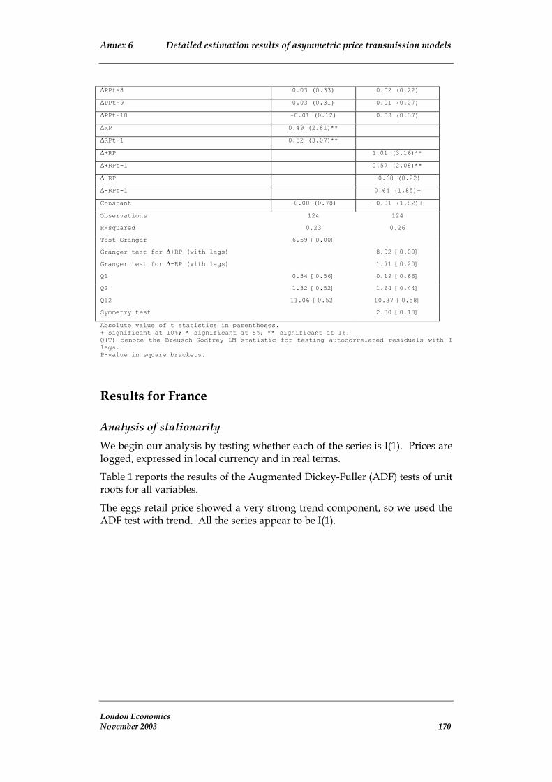
Annex 6 Detailed estimation results of asymmetric price transmission models
∆PPt-8 0.03 (0.33) 0.02 (0.22)
∆PPt-9 0.03 (0.31) 0.01 (0.07)
∆PPt-10 -0.01 (0.12) 0.03 (0.37)
∆RP 0.49 (2.81)**
∆RPt-1 0.52 (3.07)**
∆+RP 1.01 (3.16)**
∆+RPt-1 0.57 (2.08)**
∆-RP -0.68 (0.22)
0.64 (1.85)+
Constant -0.00 (0.78) -0.01 (1.82)+
Observations 124 124
R-squared 0.23 0.26
6.59 [0.00]
Granger test for ∆+RP (with lags) 8.02 [0.00]
Granger test for ∆-RP (with lags) 1.71 [0.20]
Q1 0.34 [0.56] 0.19 [0.66]
Q2 1.32 [0.52] 1.64 [0.44]
Q12 11.06 [0.52] 10.37 [0.58]
Symmetry test 2.30 [0.10]
∆-RPt-1
Test Granger
Absolute value of t statistics in parentheses. + significant at 10%; * significant at 5%; ** significant at 1%. Q(T) denote the Breusch-Godfrey LM statistic for testing autocorrelated residuals with T lags.
We begin our analysis by testing whether each of the series is I(1). Prices are logged, expressed in local currency and in real terms.
P-value in square brackets.
Results for France
Analysis of stationarity
Table 1 reports the results of the Augmented Dickey-Fuller (ADF) tests of unit roots for all variables.
The eggs retail price showed a very strong trend component, so we used the ADF test with trend. All the series appear to be I(1).
London Economics November 2003 170

Annex 6 Detailed estimation results of asymmetric price transmission models
Table A.33: Results of ADF test
PP RP
Original Series
First Difference
Original Series
First Difference
-1.04 (4) -10.45* (0) -17.06* (0)
Wheat/Bread -0.90 (12) -3.15* (11) -1.75 (12) -10.14* (0)
Lamb -2.45 (1) -7.71* (4) -0.77 (1) -11.19* (0)
Eggs -2.81 (0) -12.42* (0) 0.13t (0) -11.59t* (0)
Chicken -0.52 (2) -10.76* (1) -1.98 (0) -9.23* (0)
Beef -0.81 (1)
Lag length selected on the basis of the AIC. t denotes ADF test with a trend. * Rejection of the null hypothesis of non-stationarity PP producer prices, RP retail prices
Cointegration: estimation of a long-run relationship We have tried several long-run specifications for each one of the analysed products. The deseasonalised series for wheat/bread, beef, chicken, lamb, and eggs long-run relationship shows non-stationarity of the residuals under different specifications.
Eggs According to the AIC criterion, any model that excludes the producer prices is superior to the models that include the producer prices with any lags. However, for illustrative purposes we report the best model (according to AIC) among those that include the producer prices. Not surprisingly, the producer prices (whether allowing for asymmetries or not) are not statistically significant. Therefore, there is no Granger-causality from farm to retail prices.
In the equation for producer prices selected on the basis of the AIC we observe that consumer prices seem to be affecting producer prices (F test 4.68 with p-value 0.00). When allowing for asymmetry we see that symmetry cannot be rejected.
Hence, Granger-causality tests suggest that causality runs only in one direction and asymmetrically. Consumer prices are affecting farm prices, but there is no effect from producer prices to consumer prices.
Estimates of the models for Eggs (retail prices) Symmetric Asymmetric
∆RPt-1 -0.03 (0.37) -0.03 (0.32)
∆RPt-2 0.06 (0.66) 0.06 (0.62)
London Economics November 2003 171

Annex 6 Detailed estimation results of asymmetric price transmission models
∆RPt-3 0.11 (1.17) 0.11 (1.07)
∆RPt-4 0.06 (0.68) 0.07 (0.67)
∆RPt-5 -0.05 (0.53) -0.03 (0.26)
∆RPt-6 -0.06 (0.63) -0.04 (0.36)
∆RPt-7 -0.07 (0.70) -0.01 (0.13)
∆RPt-8 0.06 (0.63) 0.10 (0.95)
∆RPt-9 0.16 (1.68)+ 0.16 (1.56)
∆RPt-10 0.22 (2.28)* 0.15 (1.47)
-0.13 (1.40)
0.27 (2.82)**
(0.14)
∆PPt-1 0.01 (1.35)
∆PPt-2 0.01 (1.35)
∆PPt-3 0.01 (1.56)
∆PPt-4 0.01 (0.89)
∆PPt-5 -0.00 (0.20)
∆PPt-6 0.00 (0.01)
∆PPt-7 0.00 (0.21)
∆PPt-8 0.02 (2.44)*
∆PPt-9 0.02 (2.26)*
∆PPt-10 0.01 (1.74)+
∆+PPt -0.01 (0.37)
∆+PPt-1 0.01 (0.65)
∆+PPt-2 0.00 (0.11)
∆+PPt-3 0.02 (1.58)
∆+PPt-4 0.03 (1.91)+
∆+PPt-5 0.00 (0.01)
∆+PPt-6 -0.00 (0.14)
∆+PPt-7 0.00 (0.07)
∆+PPt-8 0.04 (2.47)*
∆+PPt-9 0.00 (0.14)
∆+PPt-10 0.00 (0.30)
∆-PPt -0.00 (0.11)
∆-PPt-1 0.02 (0.96)
∆-PPt-2 0.02 (0.98)
∆-PPt-3 -0.00 (0.29)
∆-PPt-4 -0.02 (1.12)
∆-PPt-5 -0.00 (0.16)
∆-PPt-6 -0.01 (0.35)
∆-PPt-7 -0.00 (0.07)
∆-PPt-8 0.00 (0.08)
∆-PPt-9 0.03 (2.18)*
∆-PPt-10 0.01 (0.81)
Constant 0.00 (0.62) -0.00 (0.53)
Observations 135 135
R-squared 0.32 0.37
Test Granger 1.64 [0.10]
Q2 0.67 [0.72] 0.90 [0.64]
∆RPt-11 -0.14 (1.44)
∆RPt-12 0.29 (2.80)**
∆PP -0.00
London Economics November 2003 172

Annex 6 Detailed estimation results of asymmetric price transmission models
Q12 12.89 [0.38] 14.35 [0.28]
F test positives 1.34 [0.21]
F test negatives 0.75 [0.68]
Asymmetry test 0.67 [0.76]
Absolute value of t statistics in parentheses. + significant at 10%; * significant at 5%; ** significant at 1%. Q(T) denote the Breusch-Godfrey LM statistic for testing autocorrelated residuals with T lags. P-value in square brackets.
Estimates of the models for Eggs (producer prices) PRODUCER EGGS Symmetric Asymmetric
∆RP -1.68 (1.67)+ --
∆RPt-1 0.81 (0.81) --
∆RPt-2 -1.43 (1.41) --
∆RPt-3 3.67 (3.64)** --
∆+RPt -- 0.27 (0.12)
∆+RPt-1 -- -3.37 (1.52)
∆+RPt-2 -- 1.11 (0.51)
∆+RPt-3 -- 2.62 (1.19)
∆-RPt -- -2.68 (1.63)
∆-RPt-1 -- 3.18 (1.92)+
∆-RPt-2 -- -2.69 (1.58)
∆-RPt-3 -- 4.28 (2.58)*
Constant -0.00 (0.90) -0.00 (0.12)
Observations 144 144
R-squared 0.12 0.16
Test Granger 4.68 [0.00] --
Q1 0.01 [0.93] 0.32 [0.57]
Q2 0.11 [0.95] 0.93 [0.63]
Q12 4.69 [0.97] 5.01 [0.96]
F test positives -- 0.92 [0.46]
F test negatives -- 4.87 [0.00]
Symmetry test -- 1.72 [0.15]
Absolute value of t statistics in parentheses. + significant at 10%; * significant at 5%; ** significant at 1%. Q(T) denote the Breusch-Godfrey LM statistic for testing autocorrelated residuals with T lags. P-value in square brackets.
Chicken The equation for consumer prices shows Granger-causality from producer prices. However, no differences can be reported when allowing different parameters for increases and decreases (F tests 0.55 and 1.92 for increases and decreases, respectively).
The equation for producer prices shows Granger-causality from consumer prices (F test 2.63) but, again, no differences for increases (F test 1.17, p-value 0.32) or decreases (F test 0.48, p-value 0.86) can be found.
London Economics November 2003 173

Annex 6 Detailed estimation results of asymmetric price transmission models
Estimates of the models for Chicken (retail prices) CHICKEN RETAIL Symmetric Asymmetric
∆PP 0.02 (2.05)* --
∆+PP -- 0.01 (0.74)
∆-PP -- 0.03 (1.38)
Constant -0.00 (3.47)** -0.00 (1.77)+
Observations 107 107
R-squared 0.04 0.04
Test Granger 4.21 [0.04] --
Q1 0.10 [0.76] 0.09 [0.76]
Q2 0.09 [0.95] 0.09 [0.96]
Q12 10.53 [0.57] 10.46 [0.58]
F test positives -- 0.55 [0.46]
F test negatives -- 1.92 [0.17]
Symmetry test -- 0.16 [0.69]
Absolute value of t statistics in parentheses. + significant at 10%; * significant at 5%; ** significant at 1%. Q(T) denote the Breusch-Godfrey LM statistic for testing autocorrelated residuals with T lags. P-value in square brackets.
Estimates of the models for Chicken (producer prices) Symmetric Asymmetric
∆PPt-1 -0.27 (2.64)** -0.27 (2.48)*
∆PPt-2 -0.17 (1.58) -0.18 (1.67)+
∆RP 2.17 (2.40)* --
∆RPt-1 0.52 (0.56) --
∆RPt-2 -0.83 (0.90) --
∆RPt-3 -0.10 (0.11) --
∆RPt-4 1.95 (2.13)* --
∆RPt-5 -2.11 (2.30)* --
∆RPt-6 -0.07 (0.07) --
∆RPt-7 -1.26 (1.35) --
∆+RPt -- 5.86 (2.11)*
∆+RPt-1 -- 0.05 (0.02)
∆+RPt-2 -- -3.32 (1.10)
∆+RPt-3 -- 0.76 (0.25)
∆+RPt-4 -- 3.67 (1.22)
∆+RPt-5 -- -5.23 (1.70)+
-- 1.51 (0.49)
∆+RPt-7 -- -1.91 (0.66)
∆-RPt -- 1.06 (0.75)
∆-RPt-1 -- 0.35 (0.25)
∆-RPt-2 -- -0.30 (0.21)
∆-RPt-3 -- -0.08 (0.05)
∆-RPt-4 -- 1.69 (1.20)
∆-RPt-5 -- -1.01 (0.70)
∆+RPt-6
London Economics November 2003 174

Annex 6 Detailed estimation results of asymmetric price transmission models
∆-RPt-6 -- -0.58 (0.41)
∆-RPt-7 -- -1.10 (0.79)
Constant -0.01 (1.01) -0.01 (0.49)
Observations 100 100
R-squared 0.27 0.30
Test Granger 2.63 [0.01] --
Q1 1.03 [0.31] 2.42 [0.12]
Q2 2.17 [0.34] 2.89 [0.24]
Q12 13.66 [0.32] 17.18 [0.14]
F test positives -- 1.17 [0.33]
F test negatives -- 0.48 [0.87]
Symmetry test -- 0.45 [0.89]
Absolute value of t statistics in parentheses. + significant at 10%; * significant at 5%; ** significant at 1%. Q(T) denote the Breusch-Godfrey LM statistic for testing autocorrelated residuals with T lags. P-value in square brackets.
Lamb The equation for consumer prices shows no Granger-causality from producer prices, even after allowing for differences in increases or decreases.
Producer prices do seem not to be affected by consumer prices. Differences in increases and decreases are not statistically different (symmetry test shows F 1.00, p-value 0.37).
Estimates of the models for Lamb (retail prices) Symmetric Asymmetric
∆PP 0.03 (1.65) --
∆+PP -- 0.03 (0.73)
∆-PP -- 0.04 (1.10)
Constant -0.00 (0.13) 0.00 (0.08)
Observations 176 176
R-squared 0.02 0.02
Test Granger 2.73 [0.10] --
Q1 1.30 [0.25] 1.33 [0.25]
Q2 1.41 [0.49] 1.43 [0.49]
Q12 9.46 [0.66] 9.89 [0.63]
F test positives -- 0.53 [0.47]
F test negatives -- 1.21 [0.27]
Symmetry test -- 0.05 [0.82]
Absolute value of t statistics in parentheses. + significant at 10%; * significant at 5%; ** significant at 1%. Q(T) denote the Breusch-Godfrey LM statistic for testing autocorrelated residuals with T lags. P-value in square brackets.
London Economics November 2003 175
Estimates of the models for Lamb (producer prices) Symmetric Asymmetric

Annex 6 Detailed estimation results of asymmetric price transmission models
∆PPt-1 0.19 (2.43)* 0.18 (2.28)*
∆PPt-2 -0.10 (1.26) -0.11 (1.36)
∆PPt-3 -0.10 (1.30) -0.12 (1.45)
∆PPt-4 -0.11 (1.37) -0.12 (1.53)
∆PPt-5 -0.18 (2.25)* -0.18 (2.34)*
∆RPt 0.41 (1.46) --
∆RPt-1 0.44 (1.57) --
∆+RPt -- 0.68 (1.42)
∆+RPt-1 -- 0.80 (1.65)
∆-RPt -- 0.00 (0.01)
∆-RPt-1 -- 0.08 (0.17)
Constant 0.00 (0.40) -0.00 (0.81)
Observations 171 171
R-squared 0.15 0.16
Test Granger 2.53 [0.08] --
Q1 0.21 [0.65] 0.33 [0.56]
Q2 0.34 [0.84] 0.35 [0.84]
Q12 7.05 [0.85] 8.18 [0.77]
F test positives -- 3.19 [0.04]
F test negatives -- 0.01 [0.99]
Symmetry test -- 1.00 [0.37]
Absolute value of t statistics in parentheses. + significant at 10%; * significant at 5%; ** significant at 1%. Q(T) denote the Breusch-Godfrey LM statistic for testing autocorrelated residuals with T lags. P-value in square brackets.
Bread The consumer equation for bread shows Granger-causality from wheat prices. However, when allowing for differences in price increases and decreases, only increases seem to have an effect (F test 3.42, p-value 0.00) but not decreases (F test 1.83, p-value 0.09). Such differences are statistically significant (symmetry test shows F test 2.57 with p-value 0.02).
The equation for producer prices selected on the basis of the AIC criterion uses twelve lags for the dependent variable and just the contemporaneous retail prices. The F test suggest that consumer prices are not affecting farm prices at a 5% level of confidence. Moreover, there seems to be no difference between increases and decreases.
Estimates of the models for Bread (retail prices) ∆PP 0.01 (1.65) --
∆PPt-1 0.01 (1.83)+ --
∆PPt-2 0.00 (0.79) --
∆PPt-3 0.01 (2.57)* --
∆PPt-4 -0.01 (1.55) --
∆PPt-5 0.00 (0.99) --
∆PPt-6 0.01 (1.65) --
London Economics November 2003 176

Annex 6 Detailed estimation results of asymmetric price transmission models
∆+PPt -- 0.01 (1.03)
∆+PPt-1 -- 0.03 (4.29)**
∆+PPt-2 -- -0.00 (0.58)
∆+PPt-3 -- 0.01 (1.52)
∆+PPt-4 -- -0.01 (1.04)
∆+PPt-5 -- 0.01 (0.91)
∆+PPt-6 -- 0.01 (0.96)
∆-PPt -- 0.01 (1.27)
∆-PPt-1 -- -0.01 (1.39)
∆-PPt-2 -- 0.01 (1.33)
0.01 (2.41)*
∆-PPt-4 -- -0.00 (0.52)
∆-PPt-5 -- 0.00 (0.18)
∆-PPt-6 -- 0.01 (1.17)
Constant 0.00 (1.93)+ -0.00 (0.14)
Observations 147 147
R-squared 0.11 0.22
Test Granger 2.50 [0.02] --
Q1 1.21 [0.27] 3.17 [0.07]
Q2 1.11 [0.57] 3.02 [0.22]
Q12 14.57 [0.27] 16.70 [0.16]
F test positives -- 3.42 [0.00]
F test negatives -- 1.83 [0.09]
Symmetry test -- 2.57 [0.02]
∆-PPt-3 --
Absolute value of t statistics in parentheses. + significant at 10%; * significant at 5%; ** significant at 1%. Q(T) denote the Breusch-Godfrey LM statistic for testing autocorrelated residuals with T lags. P-value in square brackets.
Estimates of the models for Bread (producer prices) Symmetric Asymmetric
∆PPt-1 0.03 (0.36) 0.05 (0.64)
∆PPt-2 -0.15 (1.84)+ -0.15 (1.93)+
∆PPt-3 -0.11 (1.32) -0.12 (1.45)
∆PPt-4 -0.06 (0.79) -0.06 (0.68)
∆PPt-5 -0.11 (1.36) -0.10 (1.27)
∆PPt-6 -0.12 (1.47) -0.13 (1.63)
∆PPt-7 -0.06 (0.69) -0.07 (0.89)
∆PPt-8 -0.08 (1.01) -0.07 (0.87)
∆PPt-9 -0.06 (0.78) -0.07 (0.81)
∆PPt-10 -0.11 (1.27) -0.10 (1.23)
∆PPt-11 0.01 (0.08) 0.00 (0.03)
∆PPt-12 0.40 (4.84)** 0.39 (4.59)**
∆RP 2.70 (1.70)+ --
∆+RP -- -0.35 (0.13)
∆-RP -- 6.82 (2.01)*
Constant -0.01 (1.87)+ -0.00 (0.17)
Observations 147 147
PRODUCER BREAD
London Economics November 2003 177

Annex 6 Detailed estimation results of asymmetric price transmission models
R-squared 0.27 0.28
Test Granger 2.89 [0.09] --
Q1 1.93 [0.17] 1.25 [0.26]
Q2 5.11 [0.08] 3.48 [0.18]
Q12 9.07 [0.70] 11.26 [0.51]
F test positives -- 0.02 [0.90]
F test negatives -- 4.05 [0.05]
Symmetry test -- 1.89 [0.17]
Absolute value of t statistics in parentheses. + significant at 10%; * significant at 5%; ** significant at 1%. Q(T) denote the Breusch-Godfrey LM statistic for testing autocorrelated residuals with T lags. P-value in square brackets.
Beef There does not seem to be Granger-causality from farm prices in the consumer equation. The results do not change when we allow for price asymmetry.
The same result holds for the producer prices equation. There is no effect from retail prices, even after allowing for asymmetric short-run transmission.
Estimates of the models for Beef (retail prices) Symmetric Asymmetric
∆RPt-1 -0.22 (3.02)** -0.22 (3.03)**
∆RPt-2 0.11 (1.47) 0.11 (1.50)
0.09 (1.19) 0.09 (1.24)
∆PP 0.01 (0.81) --
∆+PP -- -0.01 (0.17)
∆-PP -- 0.03 (1.08)
Constant -0.00 (0.29) 0.00 (0.27)
R-squared 0.07 0.07
Test Granger 0.65 [0.42] --
Q1 0.09 [0.76] 1.71 [0.19]
Q2 0.39 [0.82] 1.72 [0.42]
Q12 18.24 [0.11] 22.84 [0.03]
F test positives -- 0.03 [0.86]
F test negatives -- 1.16 [0.28]
Symmetry test --
∆RPt-3
Observations 189 189
0.54 [0.46]
Absolute value of t statistics in parentheses. + significant at 10%; * significant at 5%; ** significant at 1%. Q(T) denote the Breusch-Godfrey LM statistic for testing autocorrelated residuals with T lags. P-value in square brackets.
Estimates of the models for Beef (producer prices)
0.26 (3.68)**
Symmetric Asymmetric
∆PPt-1 0.26 (3.68)**
London Economics November 2003 178

Annex 6 Detailed estimation results of asymmetric price transmission models
∆RP 0.24 (0.79) --
--
∆-RP -- 0.10 (0.18)
-0.00 (0.88) -0.00 (0.81)
191
R-squared 0.07 0.07
Test Granger 0.62 [0.43] --
Q1 1.01 [0.31] 1.01 [0.31]
Q2 1.22 [0.54] 1.12 [0.57]
Q12 11.28 [0.50] 11.14 [0.52]
F test positives -- 0.46 [0.50]
F test negatives -- 0.03 [0.86]
-- 0.09 [0.76]
∆+RP 0.39 (0.68)
Constant
Observations 191
Symmetry test
Absolute value of t statistics in parentheses. + significant at 10%; * significant at 5%; ** significant at 1%. Q(T) denote the Breusch-Godfrey LM statistic for testing autocorrelated residuals with T lags. P-value in square brackets.
Results for Germany
Analysis of stationarity We begin our analysis by testing whether each of the series is I(1). Prices are logged, expressed in local currency and in real terms. Farm prices for potatoes were missing in months 6 and 7, therefore we excluded those months for the analysis of potatoes.
Table 1 reports the results of the Augmented Dickey-Fuller (ADF) tests of unit roots for all variables. For prices that appeared to be trended, an ADF test with trend was used. We have found that all series are I(1) except for carrots that has been found to be I(0). Apples39, potatoes, lamb, chicken and eggs prices farm prices are all I(1).
39 The results of the ADF test for producer apple prices were a bit different depending on the criterion used for lag selection. However, additional KPSS tests for different lags corroborated the result of I(1).
London Economics November 2003 179

Annex 6 Detailed estimation results of asymmetric price transmission models
Table A.34: Results of ADF test
PP RP
Original Series
First Difference
Original Series
First Difference
-4.16* (0) -- -3.86* (1)
Potatoes -1.93 (0) -8.09* (0) -2.47 (1) -6.76* (0)
Apples -2.26 (2) -11.95* (1) -2.39 (3) -5.85* (3)
-2.26t (12) -4.03t* (12) -3.79t* (6)
Chicken -2.30 (2) -3.82* (3) -1.43 (3) -4.70* (2)
Carrots --
Lamb -3.01t (9)
Lag length selected on the basis of the AIC.
PP producer prices, RP retail prices
Cointegration: estimation of a long-run relationship We have tried several long-run specifications for each one of the analysed products. The results for the retail-producer long-run relationship (equation 1) are presented in Table 2:
t denotes ADF test with a trend. * Rejection of the null hypothesis of non-stationarity
• In the long-run relationship the deseasonalised series for chicken, lamb, potatoes and eggs shows non-stationarity of the residuals under different specifications.
• The deseasonalised series for apples and carrots shows stationary residuals in the long-run relationship.
London Economics November 2003 180

Annex 6 Detailed estimation results of asymmetric price transmission models
Table A.35: Retail-producer long-run equations.
Chain analysed Long-run equation ADF1 test for
stationarity of û1t (lags)
Sample period
Chicken(d) PRt =1.41+0.50PPt + u1t -2.11 (0) 1993m1-2002m3
Apples(d) PRt =1.29+0.51PPt + u1t -3.50* (0) 1987m1-2002m3
Eggs(d) PRt = 0.37+1.07PPt + u1t -2.87 (0) 1993m1-2002m2
Carrots(d) PRt = 0.81+0.40PPt + u1t -4.88* (0) 1993m1-2002m3
Lamb(d) PRt =1.93+0.44PPt + u1t -0.24 (4) 1985m6-2002m3
Potatoes(d) PRt = 1.33+0.26PPt + u1t -2.16 (0) 1993m1-2002m3
1 Model chosen on the basis of AIC criterion. 2 Deseasonalised series are indicated by (d).
The results for the producer-retail long-run relationship are presented in Table A.36, and show similar cointegration results than the previous table.
* Residuals stationary (rejection of null hypothesis of non-stationarity at 95% level).
London Economics November 2003 181

Annex 6 Detailed estimation results of asymmetric price transmission models
Table A.36: Producer-retail long-run equations.
Chain analysed Long-run equation ADF1 test for
stationarity of û1t (lags)
Sample period
Chicken(d) PPt =-1.92+1.53PRt + u2t -2.08 (0) 1993m1-2002m3
PPt =-2.01+1.53PRt + u2t -4.53* (2)
Eggs(d) PPt = -0.16+0.74PRt + u2t -2.53 (0) 1993m1-2002m2
Carrots(d) PPt = -1.39+1.29PRt + u2t -6.27* (0) 1993m1-2002m3
Lamb(d) PPt = 0.94+0.38PRt + u2t -2.84 (2) 1985m6-2002m3
Potatoes(d) PPt = -4.57+3.20PRt + u2t -2.23 (0) 1993m1-2003m2
Apples(d) 1987m1-2002m3
1 Model chosen on the basis of AIC criterion. 2 Deseasonalised series are indicated by (d). * Residuals stationary (rejection of null hypothesis of non-stationarity at 95% level).
In the next sections we present the results of the error correction models for retail and producer models. For purposes of comparison, estimates of both asymmetric and symmetric error correction models are presented for the retail price and producer price models.
Apples The t-statistics for ECTt-1 in the column for retail price indicate that retail prices respond to shocks that make the relationship deviate from the long-run equilibrium.
When allowing for asymmetric transmission we observe that both ECT+t-1 and ECT-t-1 are statistically significant but we cannot reject the hypothesis that the parameters are equal. This provides evidence of symmetric price transmission.
The equation of farm prices shows there is a long-run relationship (evidence of transmission) but when allowing for asymmetric transmission we observe that the symmetry of the parameters cannot be rejected at a 5% level.
The Granger-causality tests suggest that transmission is bi-directional, in the sense that farm prices are affecting consumer prices but consumer prices are also affecting farm prices.
London Economics November 2003 182

Annex 6 Detailed estimation results of asymmetric price transmission models
Estimates of the Error correction models for Apples (retail prices) RP APLES Symmetric Asymmetric
∆RPt-1 0.44 (6.39)** 0.44 (6.35)**
∆RPt-2 -0.23 (3.06)** -0.23 (3.00)**
∆RPt-3 0.20 (2.69)** 0.20 (2.65)**
∆RPt-4 -0.12 (1.57) -0.12 (1.61)
∆RPt-5 0.05 (0.73) 0.05 (0.69)
0.07 (0.90) 0.07 (0.89)
∆RPt-7 -0.02 (0.24) -0.01 (0.17)
∆RPt-8 0.07 (0.99) 0.07 (1.04)
∆PPt 0.14 (7.13)** 0.14 (7.16)**
∆PPt-1 0.02 (0.78) 0.01 (0.71)
∆PPt-2 0.04 (1.84)+ 0.03 (1.77)+
ECTt-1 -0.14 (3.90)**
ECT+t-1 -0.18 (2.99)**
ECT-t-1
-0.00 (0.09) 0.00 (0.57)
Observations 174 174
R-squared 0.47 0.47
16.02 [0.00] 12.93 [0.00]
Q1 0.82 [0.36] 1.20 [0.27]
Q2 4.14 [0.13] 4.56 [0.10]
Q12 13.87 [0.31] 13.07 [0.36]
Symmetry test 0.70 [0.41]
∆RPt-6
-0.11 (2.05)*
Constant
Test Granger
Absolute value of t statistics in parentheses + significant at 10%; * significant at 5%; ** significant at 1% Q(T) denote the Breusch-Godfrey LM statistic for testing autocorrelated residuals with T lags. P-value in square brackets
Estimates of the Error correction models for Apples (producer prices) Symmetric Asymmetric
∆PPt-1 -0.12 (1.17) -0.12 (1.14)
∆PPt-2 -0.22 (2.08)* -0.22 (2.10)*
∆PPt-3 -0.11 (1.06) -0.12 (1.15)
∆PPt-4 -0.07 (0.68) -0.08 (0.79)
-0.07 (0.69) -0.08 (0.81)
∆PPt-6 -0.01 (0.14) -0.02 (0.19)
∆PPt-7 0.00 (0.05) -0.00 (0.03)
0.07 (0.84) 0.07 (0.88)
∆PPt-9 0.13 (1.78)+ 0.12 (1.76)+
∆RPt 1.75 (7.10)** 1.72 (7.00)**
-0.13 (0.43) -0.09 (0.28)
∆RPt-2 0.45 (1.44) 0.43 (1.39)
PP APLES
∆PPt-5
∆PPt-8
∆RPt-1
London Economics November 2003 183

Annex 6 Detailed estimation results of asymmetric price transmission models
∆RPt-3 -0.12 (0.37) -0.07 (0.22)
0.33 (1.06) 0.34 (1.12)
∆RPt-5 -0.08 (0.26) -0.04 (0.14)
∆RPt-6 -0.16 (0.56) -0.17 (0.57)
∆RPt-7 -0.14 (0.48) -0.14 (0.51)
∆RPt-8 -0.31 (1.21) -0.31 (1.22)
ECTt-1 -0.27 (2.90)**
ECT+t-1 -0.12 (0.92)
ECT-t-1 -0.46 (3.26)**
Constant -0.00 (0.07) -0.02 (1.43)
Observations 174 174
R-squared 0.37 0.38
Test Granger 7.92 [0.00] 7.58 [0.00]
Q1 1.02 [0.31] 0.77 [0.38]
Q2 4.48 [0.11] 4.06 [0.13]
Q12 16.34 [0.18] 14.14 [0.29]
Symmetry test 3.10 [0.08]
∆RPt-4
Absolute value of t statistics in parentheses + significant at 10%; * significant at 5%; ** significant at 1% Q(T) denote the Breusch-Godfrey LM statistic for testing autocorrelated residuals with T lags. P-value in square brackets
Chicken Although the series for retail and producer prices are I(1), there is no long-run relationship between retail and farm chicken deseasonalised prices. Using several specifications we were unable to reject non-stationarity of the residuals.
We have proceeded to estimate the models in first differences but without inclusion of the error correction term. In a further step we have tested for Granger-causality.
The first model for retail prices uses only the current price of farm prices and three lags. The F test indicates that the prices for chicken are jointly statistically significant different from zero (F value is 14.47 with a p-value of 0.00).
In a second model we have allowed for different coefficients for increases of the current and lagged wheat prices. The F statistics show that increases and decreases are statistically significant. Moreover, we can reject at a 5% level that the parameters for increases are equal than for decreases. This is evidence of asymmetry.
For farm prices, we have chosen the optimal lag specification using the AIC criterion ensuring no autocorrelated residuals. The results show that consumer prices are affecting producer prices (F test is 20.27 with p-value 0.00). In a second model we have allowed for different coefficients for London Economics November 2003 184

Annex 6 Detailed estimation results of asymmetric price transmission models
increases of the current and lagged wheat prices. The symmetry test cannot be rejected.
Estimates of the models for Chicken (retail prices) RP CHICKEN Symmetric Asymmetric
∆PPt 0.26 (4.60)**
∆PPt-1 0.03 (0.49)
∆PPt-2 0.01 (0.19)
∆PPt-3 0.17 (2.99)**
∆+PPt 0.24 (2.75)**
∆+PPt-1 -0.01 (0.12)
∆+PPt-2 0.07 (0.78)
∆+PPt-3 0.36 (4.05)**
∆-PPt 0.28 (3.25)**
∆-PPt-1 0.05 (0.54)
∆-PPt-2 -0.05 (0.55)
∆-PPt-3 -0.03 (0.28)
Constant 0.00 (0.00) -0.00 (1.66)
Observations 107 107
R-squared 0.36 0.43
Test Granger 14.47 [0.00]
Q1 0.06 [0.80] 1.01 [0.31]
Q2 2.21 [0.33] 1.61 [0.45]
Q12 6.98 [0.86] 8.81 [0.72]
F test positives 9.61 [0.00]
F test negatives 3.25 [0.01]
Symmetry test 2.83 [0.03]
Absolute value of t statistics in parentheses + significant at 10%; * significant at 5%; ** significant at 1% Q(T) denote the Breusch-Godfrey LM statistic for testing autocorrelated residuals with T lags. P-value in square brackets
Estimates of the models for Chicken (producer prices) ∆PP Symmetric Asymmetric
∆PPt-1 0.20 (2.22)* 0.21 (2.32)*
∆PPt-2 0.22 (2.52)* 0.23 (2.61)*
∆RP 0.62 (4.50)**
∆+RP 0.45 (1.59)
∆-RP 0.74 (3.48)**
Constant -0.00 (0.51) 0.00 (0.24)
Observations 108 108
R-squared 0.38 0.38
Test Granger 20.27 [0.00]
Q1 1.94 [0.16] 1.23 [0.27]
Q2 3.73 [0.15] 3.24 [0.20]
Q12 8.09 [0.78] 7.89 [0.79]
F test positives 2.53 [0.11]
London Economics November 2003 185

Annex 6 Detailed estimation results of asymmetric price transmission models
F test negatives 12.10 [0.00]
Symmetry test 0.53 [0.47]
Absolute value of t statistics in parentheses + significant at 10%; * significant at 5%; ** significant at 1% Q(T) denote the Breusch-Godfrey LM statistic for testing autocorrelated residuals with T lags. P-value in square brackets
Carrots The series for retail and producer prices are I(0) after deseasonalisation. We have estimated the error correction model with the prices in levels. In a further step we tested for Granger-causality.
In the equation for consumer prices we are using two lags for the dependent variable, and the contemporaneous farm price. For the producer price we have used the contemporaneous value and one lag for the consumer price.
The t-statistics for the ECTt-1 indicates that the retail price does not respond to long-run deviations (whether symmetric or asymmetric). However, we cannot reject significance of the short-run effects.
The result for the farm prices equation is the following. There is evidence of transmission (the absolute t-statistic for ECTt-1 is 4.29) and moreover the symmetry test suggests that the transmission is asymmetric with a stronger adjustment of positive deviations from the long-term equilibrium.
Estimates of the models for Carrots (consumer prices) RP CARROTS Symmetric Asymmetric
RPt-1 1.10 (11.56)** 1.09 (11.44)**
RPt-2 -0.35 (4.37)** -0.35 (4.32)**
PPt 0.12 (5.22)** 0.12 (5.26)**
ECTt-1 0.03 (0.55)
ECT+t-1 -0.01 (0.14)
ECT-t-1 0.11 (1.01)
Constant 0.22 (5.33)** 0.22 (5.39)**
Observations 107 107
R-squared 0.92 0.92
Test Granger 14.95 [0.00] 10.18 [0.00]
Q1 0.36 [0.55] 0.46 [0.50]
Q2 1.31 [0.52] 1.47 [0.48]
Q12 9.59 [0.65] 11.70 [0.47]
Symmetry test 0.73 [0.39]
Absolute value of t statistics in parentheses + significant at 10%; * significant at 5%; ** significant at 1% Q(T) denote the Breusch-Godfrey LM statistic for testing autocorrelated residuals with T lags. P-value in square brackets
Estimates of the models for Carrots (producer prices) PP CARROTS Symmetric Asymmetric
London Economics November 2003 186

Annex 6 Detailed estimation results of asymmetric price transmission models
RP 1.90 (6.42)** 1.92 (6.62)**
RPt-1 -0.68 (2.33)* -0.74 (2.57)*
ECTt-1 0.38 (4.29)**
0.71 (4.22)**
ECT-t-1 0.12 (0.82)
Constant -1.35 (22.44)** -1.36 (22.99)**
Observations 107 107
R-squared 0.63 0.65
Test Granger 59.15 [0.00] 47.44 [0.00]
Q1 0.61 [0.44] 0.39 [0.53]
Q2 1.88 [0.39] 1.68 [0.43]
Q12 10.89 [0.54] 9.98 [0.62]
Symmetry test 5.15 [0.03]
ECT+t-1
Absolute value of t statistics in parentheses + significant at 10%; * significant at 5%; ** significant at 1% Q(T) denote the Breusch-Godfrey LM statistic for testing autocorrelated residuals with T lags. P-value in square brackets
Potatoes Although the series for retail and producer prices are I(1), we have not found a long-run relationship between deseasonalised retail and farm potatoes prices. Using several specifications we were unable to reject non-stationarity of the residuals.
We have proceeded to estimate the models in first differences but without inclusion of the error correction term. In a further step we have tested for Granger-causality.
The first model for retail prices uses only the current farm price and one additional lag. The F test indicates that the prices for potatoes are jointly statistically significant different from zero (F value is 156.02 with a p-value of 0.00).
In a second model we have allowed for different coefficients for increases and decreases of the current and lagged prices. The F statistics show that increases and decreases are statistically significant, however, we cannot reject at a 5% level that the parameters for increases are different than for decreases. This is evidence of symmetry.
For farm prices, the results show that consumer prices are affecting producer prices (F test is 297.38 with p-value 0.00). In a second model we have allowed for different coefficients for increases of the current and lagged wheat prices. Although, both price increases and decreases seem to be statistically significant, we cannot reject the hypothesis that the parameters are not different. This is evidence of symmetry.
The Granger-causality tests suggest that causality is symmetric and bi-directional, from farmer to consumer and consumer to farmer.
London Economics November 2003 187

Annex 6 Detailed estimation results of asymmetric price transmission models
Estimates of the models for Potatoes (retail prices) ∆RP POTATOES Symmetric Asymmetric
∆PP 0.24 (17.24)**
∆PPt-1 0.04 (2.58)*
∆+PP 0.23 (9.02)**
∆+PPt-1 0.05 (2.18)*
∆-PPt 0.25 (12.72)**
∆-PPt-1 0.02 (1.21)
Constant 0.00 (0.01) -0.00 (0.09)
Observations 91 91
R-squared 0.78 0.78
Test Granger 156.02 [0.00]
Q1 0.01 [0.93] 0.02 [0.88]
Q2 0.34 [0.84] 0.25 [0.88]
Q12 12.26 [0.43] 13.37 [0.34]
F test positives 43.52 [0.00]
F test negatives 81.62 [0.00]
Symmetry test 0.66 [0.52]
Absolute value of t statistics in parentheses + significant at 10%; * significant at 5%; ** significant at 1% Q(T) denote the Breusch-Godfrey LM statistic for testing autocorrelated residuals with T lags. P-value in square brackets
Estimates of the models for Potatoes (producer prices) ∆PP POTATOES Symmetric Asymmetric
∆PPt-1 -0.10 (1.91)+ -0.09 (1.78)+
∆RP 3.20 (17.24)**
∆+RP 2.82 (9.03)**
∆-RP 3.48 (13.52)**
Constant 0.00 (0.13) 0.01 (0.91)
Observations 91 91
R-squared 0.77 0.78
Test Granger 297.38 [0.00]
Q1 0.37 [0.54] 0.12 [0.73]
Q2 0.99 [0.61] 0.49 [0.78]
Q12 10.91 [0.54] 10.52 [0.57]
F test positives 81.60 [0.00]
F test negatives 182.77 [0.00]
Symmetry test 2.34 [0.13]
Absolute value of t statistics in parentheses + significant at 10%; * significant at 5%; ** significant at 1% Q(T) denote the Breusch-Godfrey LM statistic for testing autocorrelated residuals with T lags. P-value in square brackets
London Economics November 2003 188

Annex 6 Detailed estimation results of asymmetric price transmission models
Lamb The series for consumer lamb showed very strange behaviour for the year 1998 and we decided to exclude it from the analysis.
Results for the Netherlands
Analysis of stationarity We begin our analysis by testing whether each of the series is I(1). Prices are logged, expressed in local currency and in real terms.
Table A.37 reports the results of the Augmented Dickey-Fuller (ADF) tests of unit roots for all variables. Farm prices were missing for months 5, 6, and 7 for meat and for months 6, 7, and 8 for potatoes. Therefore we excluded those months for the analysis of meat and potatoes.
We found that the price series for beef and eggs are I(1). The price series for potatoes was found to be to be I(0). The price series for bread was found to be to be I(0) after inclusion of a time trend. Finally the producer prices for chicken was found to be I(0) whereas the retail prices was found to be I(0) only after inclusion of a trend in the ADF test. In addition, the KPSS test showed that both price series for chicken are I(0). Therefore, we treat the chicken series as I(0).
Table A.37: Results of ADF test
RP
Original Series
First Difference
Original Series
First Difference
-1.79t (12) -3.05t (12) -1.85t (3) -10.59t* (2)
Bread -3.71t* (0) -- -3.62t* (0) --
-3.29* (3) -- -3.35* (1)
Eggs -2.36 (0) -7.89* (0) -2.21 (0) -8.67* (0)
Chicken -4.14* (12) -- -3.72t* (12) --
PP
Beef
Potatoes --
Lag length selected on the basis of the AIC. t denotes ADF test with a trend. * Rejection of the null hypothesis of non-stationarity PP producer prices, RP retail prices
London Economics November 2003 189

Annex 6 Detailed estimation results of asymmetric price transmission models
Cointegration: estimation of a long-run relationship We have tried several long-run specifications for each one of the analysed products. The results for the retail-producer long-run relationship are presented in Table A.38:
• The long-run relationship of the deseasonalised series for chicken and beef shows non-stationarity of the residuals under different specifications.
• The deseasonalised series for the bread equation (i.e. bread dependent on wheat) shows non-stationarity of the residuals under different specifications. However, for the wheat equation (i.e. wheat dependent on bread) we can reject non-stationarity of the residuals under the lag structure selected using the AIC criterion. Because many other specifications (including optimal SBC and HQC) indicated non-stationarity of the residuals, we concluded that the residuals are non-stationary.
• The deseasonalised series for eggs and potatoes shows stationary residuals in the long-run relationship.
Table A.38: Retail-producer long-run equations.
Chain analysed Long-run equation ADF1 test for
stationarity of û1t (lags)
Sample period
Chicken(d) PRt = 1.95+0.16PPt + u1t -2.96 (6) 1996m1-2001m12
Eggs(d) PRt = 0.97+0.38PPt + u1t -4.65* (0) 1996m1-2001m12
Bread(d) PRt = 1.33+0.13PPt + u1t -2.28 (0) 1996m1-2001m12
Beef(d) PRt = 2.44+0.20PPt + u1t -2.26 (0) 1986m1-2001m12
Potatoes(d) PRt = 0.06+0.32PPt –0.00TRENDt+ u1t -4.24* (0) 1986m1-2001m12
1 Model chosen on the basis of AIC criterion. 2 Deseasonalised series are indicated by (d). * Residuals stationary (rejection of null hypothesis of no stationarity at 95% level).
The results for the producer-retail long-run relationship are presented in Table A.39.
London Economics November 2003 190

Annex 6 Detailed estimation results of asymmetric price transmission models
Table A.39: Producer-retail long-run equations.
Long-run equation
(lags)
Sample period
Chicken(d) PPt = -5.21+2.87PRt + u2t -2.21 (6) 1996m1-2001m12
Eggs(d) PPt = -2.05+2.12PRt + u2t -4.75* (2) 1996m1-2001m12
Bread(d) PPt = -8.74+6.39PRt + u2t -4.31* (8) 1996m1-2001m12
Beef(d) PPt = -8.57+3.73PRt + u2 -1.71 (0) 1986m1-2001m12
Potatoes(d) PPt = -0.48+2.24PRt –0.00TRENDt + u2 -3.76** (0) 1986m1-2001m12
Chain analysed ADF1 test for
stationarity of û1t
1 Model chosen on the basis of AIC criterion. 2 Deseasonalised series are indicated by (d). * Residuals stationary (rejection of null hypothesis of no stationarity at 95% level). ** Residuals stationary (rejection of null hypothesis of no stationarity at 90% level).
In the next paragraphs we present the results of the error correction models for retail and producer models. For purposes of comparison, estimates of both asymmetric and symmetric error correction models are presented for the retail and the producer price models.
Bread The series for retail and producer prices are I(0) with a trend, after deseasonalisation. Since the residuals of the long-run equation are not stationary, we have estimated the models in first differences, and tested for Granger-causality.
The equation for consumer prices shows Granger-causality from producer prices. However, when allowing different parameters for increases and decreases there are no statistically significant differences.
In the equation for producer prices we report Granger-causality from consumer prices (F test 8.93 with p-value 0.00), but when allowing for differences between increases and decreases there are no statistically significant differences.
Estimates of the models for Bread-Wheat (retail prices) RP BREAD Symmetric Asymmetric
∆RPt-1 -0.21 (1.88)+ -0.18 (1.67)
∆PPt 0.06 (5.94)**
∆+PPt 0.03 (1.65)
London Economics November 2003 191

Annex 6 Detailed estimation results of asymmetric price transmission models
∆-PPt 0.08 (5.51)**
Constant -0.00 (1.84)+ -0.00 (0.31)
Observations 52 52
R-squared 0.42 0.46
Test Granger 35.31 [0.00]
Q1 0.00 0.04
Q1 0.00 [0.96] 0.04 [0.84]
Q2 0.43 [0.81] 0.14 [0.93]
Q12 4.83 [0.96] 4.77 [0.97]
F test positives 2.71 [0.11]
F test negatives 30.35 [0.00]
Symmetry test 3.16 [0.08]
Absolute value of t statistics in parentheses. + significant at 10%; * significant at 5%; ** significant at 1%. Q(T) denote the Breusch-Godfrey LM statistic for testing autocorrelated residuals with T lags. P-value in square brackets.
Estimates of the models for Wheat/bread (producer prices) PP BREAD Symmetric Asymmetric
∆RPt 6.57 (5.95)**
∆RPt-2 0.10 (0.09)
∆RPt-3 0.42 (0.38)
∆RPt-4 -2.04 (1.87)+
∆+RPt 4.62 (1.37)
∆+RPt-1 4.23 (1.26)
∆+RPt-2 -3.88 (1.20)
∆+RPt-3 -1.11 (0.34)
∆+RPt-4 -7.16 (2.22)*
∆-RPt 7.50 (4.80)**
∆-RPt-1 1.64 (1.03)
∆-RPt-2 1.36 (0.85)
(0.85)
∆-RPt-4 -0.02 (0.01)
Constant -0.00 (0.19) 0.02 (1.32)
49
R-squared 0.51 0.57
Test Granger 8.93 [0.00]
Q1 0.16 [0.68] 0.35 [0.56]
Q2 0.45 [0.80] 0.71 [0.70]
Q12 14.89 [0.25] 12.70 [0.39]
F test positives 1.70 [0.16]
F test negatives 4.63 [0.00]
Symmetry test 1.05 [0.40]
∆RPt-1 1.77 (1.59)
∆-RPt-3 1.37
Observations 49
Absolute value of t statistics in parentheses. + significant at 10%; * significant at 5%; ** significant at 1%. Q(T) denote the Breusch-Godfrey LM statistic for testing autocorrelated residuals with T lags. P-value in square brackets.
London Economics November 2003 192

Annex 6 Detailed estimation results of asymmetric price transmission models
Potatoes The series for retail and producer prices are I(0) after deseasonalisation. We have therefore estimated an error correction model in levels, and tested for Granger-causality.
In the equation for consumer prices we are using 10 lags for the retail prices and one lag and the contemporaneous producer prices. The joint hypothesis of no significance of potatoes’ farm prices is rejected at a 1% level (F test 23.16, p-value 0.00). The ECT are significant in both models but we cannot reject the symmetry test. This is evidence of symmetric transmission.
The equation for the producer price selected on the basis of the AIC criterion uses ten lags for the dependent variable and the contemporaneous and one lag of the retail price. The ECT are not statistically significant. However, the F test suggest that consumer prices are affecting farm prices.
Estimates of the models for Potatoes (retail prices) RP POTATOES Symmetric Asymmetric
1.37 (9.67)** 1.38 (9.62)**
RPt-2 0.07 (0.86) 0.07 (0.87)
RPt-3 -0.05 (0.64) -0.05 (0.64)
RPt-4 0.10 (1.15) 0.10 (1.14)
RPt-5 -0.21 (2.52)* -0.21 (2.54)*
RPt-6 0.04 (0.53) 0.03 (0.42)
RPt-7 -0.02 (0.24) -0.02 (0.24)
0.10 (1.36) 0.10 (1.37)
0.03 (0.40)
0.30 (9.15)**
PPt-1 -0.28 (4.77)** -0.29 (4.78)**
PPt-2 -0.05 (0.96) -0.05 (0.96)
-0.10 (2.02)* -0.10 (2.03)*
PPt-4 -0.01 (0.26) -0.01 (0.27)
PPt-5 0.08 (2.21)* 0.09 (2.29)*
(3.66)**
ECT+t-1 -0.58 (3.07)**
ECT-t-1 -0.69 (3.50)**
-0.08 (1.84)+ -0.09 (1.95)+
Observations 143 143
R-squared 0.92 0.92
Test Granger 23.16 [0.00] 17.42 [0.00]
Q1 1.33 [0.25] 1.36 [0.24]
Q2 3.13 [0.21] 2.80 [0.25]
Q12 13.52 [0.33] 14.92 [0.25]
Symmetry test 0.41 [0.52]
RPt-1
RPt-8
RPt-9 0.03 (0.35)
RPt-10 -0.06 (1.21) -0.06 (1.20)
PPt 0.30 (9.16)**
PPt-3
ECTt-1 -0.63
Constant
Absolute value of t statistics in parentheses. + significant at 10%; * significant at 5%; ** significant at 1%.
London Economics November 2003 193

Annex 6 Detailed estimation results of asymmetric price transmission models
Q(T) denote the Breusch-Godfrey LM statistic for testing autocorrelated residuals with T lags. P-value in square brackets.
Estimates of the models for Potatoes (producer prices) Symmetric Asymmetric
PPt-1 0.96 (4.97)** 0.97 (4.96)**
PPt-2 0.06 (0.62) 0.06 (0.59)
PPt-3 0.18 (1.96)+ 0.18 (1.94)+
-0.07 (0.74) -0.07 (0.76)
PPt-5 -0.06 (0.61) -0.06 (0.60)
PPt-6 0.05 (0.49) 0.04 (0.47)
PPt-7 0.03 (0.28) 0.03 (0.28)
PPt-8 -0.06 (0.65) -0.06 (0.63)
PPt-9 -0.14 (1.46) -0.14 (1.46)
PPt-10 0.06 (0.93) 0.07 (0.95)
RPt 1.32 (9.15)** 1.33 (9.03)**
RPt-1 -1.46 (7.22)** -1.46 (7.20)**
ECTt-1 -0.18 (0.83)
ECT+t-1 -0.22 (0.91)
ECT-t-1 -0.16 (0.71)
Constant 0.02 (0.07) 0.04 (0.16)
Observations 143 143
R-squared 0.93 0.93
Test Granger 32.96 [0.00] 31.26 [0.00]
0.04 [0.84] 0.03 [0.86]
Q2 0.48 [0.79] 0.64 [0.73]
Q12 12.33 [0.42] 11.60 [0.42]
Symmetry test 0.14 [0.70]
PP POTATOES
PPt-4
Q1
Absolute value of t statistics in parentheses. + significant at 10%; * significant at 5%; ** significant at 1%. Q(T) denote the Breusch-Godfrey LM statistic for testing autocorrelated residuals with T lags. P-value in square brackets.
Beef Although the series for retail and producer prices are I(1), there is no long-run relationship between deseasonalised retail and farm beef prices.
We have proceeded to estimate the models in first differences but without inclusion of the error correction term. In a further step we have tested for Granger-causality.
The first model for retail prices uses only two and no lags for the retail and producer price, respectively. The t test for the producer price variable rejects the hypothesis of no significance. In a second model we have allowed for different coefficients for increases and decreases in the producer price but there are no statistically significant differences. This is evidence of symmetry.
For farm prices, the results show that consumer prices are affecting producer prices (F test is 2.47 with p-value 0.05). In a second model we have allowed
London Economics November 2003 194

Annex 6 Detailed estimation results of asymmetric price transmission models
for different coefficients for increases and decreases of the current and lagged wheat prices. Only price decreases (and not increases) seem to be statistically significant at a 5% level. The symmetry test rejects the hypotheses that the parameters are equal.
Estimates of the models for Beef (retail prices) RP BEEF Symmetric Asymmetric
∆RPt-1 -0.17 (2.35)* -0.16 (2.31)*
∆RPt-2 -0.22 (3.12)** -0.21 (3.01)**
∆PPt 0.05 (2.15)*
∆+PPt -0.05 (0.83)
∆-PPt 0.08 (2.84)**
Constant -0.00 (1.16) 0.00 (0.28)
Observations 191 191
0.09 0.10
Test Granger 4.60 [0.03]
Q1 1.43 [0.23] 0.01 [0.93]
Q2 1.50 [0.47] 1.26 [0.53]
Q12 7.78 [0.80] 10.83 [0.54]
F test positives 0.70 [0.41]
F test negatives 8.05 [0.00]
3.39 [0.07]
R-squared
Symmetry test
Absolute value of t statistics in parentheses. + significant at 10%; * significant at 5%; ** significant at 1%. Q(T) denote the Breusch-Godfrey LM statistic for testing autocorrelated residuals with T lags. P-value in square brackets.
Estimates of the models for Beef (producer prices) PP BEEF Symmetric Asymmetric
∆PPt-1 0.18 (2.54)* 0.17 (2.33)*
∆PPt-2 0.03 (0.42) 0.05 (0.73)
∆PPt-3 0.10 (1.39) 0.09 (1.32)
∆PPt-4 -0.03 (0.40) -0.06 (0.84)
∆PPt-5 -0.08 (1.12) -0.07 (1.06)
∆PPt-6 -0.02 (0.35) -0.02 (0.30)
∆PPt-7 -0.02 (0.32) -0.01 (0.21)
∆PPt-8 0.03 (0.36) 0.02 (0.33)
∆PPt-9 0.10 (1.42) 0.11 (1.49)
∆PPt-10 -0.12 (1.60) -0.11 (1.43)
∆PPt-11 -0.16 (2.07)* -0.17 (2.28)*
∆PPt-12 0.59 (6.37)** 0.54 (5.86)**
∆RPt 0.08 (0.35)
∆RPt-1 -0.20 (0.90)
∆RPt-2 -0.26 (1.17)
∆RPt-3 -0.65 (2.94)**
∆+RPt -0.86 (2.14)*
London Economics November 2003 195

Annex 6 Detailed estimation results of asymmetric price transmission models
∆+RPt-1 -0.61 (1.50)
∆+RPt-2 0.04 (0.10)
∆+RPt-3 -0.57 (1.41)
∆-RPt 1.00 (2.57)*
∆-RPt-1 0.02 (0.05)
∆-RPt-2 -0.56 (1.42)
∆-RPt-3 -0.72 (1.81)+
Constant -0.00 (1.56) 0.00 (0.54)
Observations 179 179
R-squared 0.30 0.34
Test Granger 2.47 [0.05]
Q1 1.39 [0.24] 1.36 [0.24]
Q2 2.75 [0.25] 2.29 [0.32]
Q12 14.15 [0.29] 16.02 [0.19]
F test positives 2.08 [0.09]
F test negatives 3.05 [0.02]
Symmetry test 2.41 [0.05]
Absolute value of t statistics in parentheses. + significant at 10%; * significant at 5%; ** significant at 1%. Q(T) denote the Breusch-Godfrey LM statistic for testing autocorrelated residuals with T lags. P-value in square brackets.
Eggs Retail prices are cointegrated with producer prices and deviations from the long-run equilibrium are corrected to re-establish the equilibrium.
When allowing for asymmetric transmission we observe that although ECT-t-1 is statistically significant and ECT+t-1 is not, the symmetry hypotheses cannot be rejected.
The equation of farm prices shows that there is a long-run relationship (evidence of transmission). When allowing for asymmetric transmission, we observe that the differences between ECT+t-1 and ECT-t-1 are not statistically significant at 5%.
Finally, the Granger-causality tests suggest that transmission is bi-directional, in the sense that farm prices are affecting consumer prices but consumer prices are also affecting farm prices.
Estimates of the models for Eggs (retail prices) RP EGGS Symmetric Asymmetric
∆RPt-1 -0.15 (1.62) -0.16 (1.64)
∆RPt-2 -0.02 (0.28) -0.03 (0.29)
∆RPt-3 0.09 (1.05) 0.08 (0.98)
∆RPt-4 -0.16 (1.91)+ -0.16 (1.94)+
∆PPt 0.09 (2.72)** 0.09 (2.68)**
∆PPt-1 0.12 (2.64)* 0.12 (2.65)*
ECTt-1 -0.34 (3.44)**
London Economics November 2003 196

Annex 6 Detailed estimation results of asymmetric price transmission models
ECT+t-1 -0.26 (1.47)
ECT-t-1 -0.40 (2.54)*
Constant -0.00 (0.85) -0.00 (0.91)
Observations 67 67
R-squared 0.53 0.53
Test Granger 17.27 [0.00] 12.86 [0.00]
Q1 0.03 [0.86] 0.03 [0.86]
Q2 0.07 [0.97] 0.15 [0.93]
Q12 11.94 [0.45] 12.22 [0.42]
Symmetry test 0.26 [0.61]
Absolute value of t statistics in parentheses. + significant at 10%; * significant at 5%; ** significant at 1%. Q(T) denote the Breusch-Godfrey LM statistic for testing autocorrelated residuals with T lags. P-value in square brackets.
Estimates of the models for Eggs (producer prices) PP EGGS Symmetric Asymmetric
∆PPt-1 0.10 (0.58) 0.10 (0.58)
∆PPt-2 0.30 (2.00)+ 0.29 (1.94)+
∆RPt 1.00 (2.78)** 0.98 (2.66)**
∆RPt-1 -0.64 (1.68)+ -0.64 (1.68)+
ECTt-1 -0.44 (2.91)**
ECT+t-1 -0.37 (1.52)
ECT-t-1 -0.51 (2.22)*
Constant -0.00 (0.31) -0.01 (0.49)
Observations 70 70
R-squared 0.19 0.19
Test Granger 4.87 [0.00] 3.64 [0.01]
Q1 0.65 [0.42] 0.83 [0.36]
Q2 2.67 [0.26 3.25 [0.20]
Q12 9.53 [0.66] 12.28 [0.42]
Symmetry test 0.14 [0.70]
Absolute value of t statistics in parentheses. + significant at 10%; * significant at 5%; ** significant at 1%. Q(T) denote the Breusch-Godfrey LM statistic for testing autocorrelated residuals with T lags. P-value in square brackets.
Chicken The series for retail and producer prices are I(0) after deseasonalisation. We have therefore estimated the models in levels, and tested for Granger-causality.
In the equation for consumer prices we are using one lag for the dependent variable and the contemporaneous farm prices. The t statistics shows evidence that farm prices are affecting consumer prices.
The equation for producer prices selected on the basis of the AIC criterion uses only the dependent variable with three lags. Additional specifications with inclusion of the retail prices were always worse in terms of the AIC London Economics November 2003 197

Annex 6 Detailed estimation results of asymmetric price transmission models
criterion. Moreover, the statistical tests always rejected the hypothesis that the retail prices were statistical significant.
Granger-causality tests suggest that causality runs only in one direction. Farm prices are affecting consumer prices, but not the other way around.
Estimates of the models for Chicken (retail prices) RP CHICKEN Symmetric
RPt-1 0.73 (9.72)**
PPt 0.05 (2.76)**
Constant 0.53 (3.58)**
Observations 71
R-squared 0.77
Test Granger 7.59 [0.01]
Q1 1.28 [0.26]
Q2 3.55 [0.17]
Q12 17.37 [0.14]
Absolute value of t statistics in parentheses. + significant at 10%; * significant at 5%; ** significant at 1%. Q(T) denote the Breusch-Godfrey LM statistic for testing autocorrelated residuals with T lags. P-value in square brackets.
Estimates of the models for Chicken (producer prices) PR CHICKEN Symmetric
PPt-1 1.16 (16.39)**
PPt-2 -0.01 (0.12)
PPt-3 -0.15 (2.16)*
Constant 0.00 (0.97)
Observations 201
R-squared 1.00
Test Granger 268.61 [0.00]
Q1 0.59 [0.44]
Q2 1.01 [0.60]
Q12 102.58 [0.00]
Absolute value of t statistics in parentheses. + significant at 10%; * significant at 5%; ** significant at 1%. Q(T) denote the Breusch-Godfrey LM statistic for testing autocorrelated residuals with T lags. P-value in square brackets.
Results of Denmark
Analysis of stationarity We begin our analysis by testing whether each of the series is I(1). Prices are logged, expressed in local currency and in real terms.
London Economics November 2003 198

Annex 6 Detailed estimation results of asymmetric price transmission models
Table A.40 reports the results of the Augmented Dickey-Fuller (ADF) tests of unit roots for all variables. Lag selection by using AIC showed that wheat, bread, flour and egg prices are I(1). Month 5 was missing for many of the years of the potato producer price series. Hence, we deleted month 5 from the series to perform the analysis. The potato series appear to be I(1).
Table A.40: Results of ADF test
PP RP
Original Series
First Difference
Original Series
First Difference
Wheat/Bread -1.25 (12) -4.63* (11) -2.03 (0) -15.07* (0)
Wheat/Flour -1.25 (12) -4.63* (11) -0.56* (0) -14.34* (0)
Eggs -2.32 (0) -7.93* (2) -1.14 (0) -13.83* (0)
Potatoes -2.75 (0) -10.99* (0) -1.85 (0) -10.26* (0)
Lag length selected on the basis of the AIC, except for † where SBC and HQC criteria are used. t denotes ADF test with a trend. * Rejection of the null hypothesis of non-stationarity PP producer prices, RP retail prices
Cointegration: estimation of a long-run relationship We have tried several long-run specifications for each one of the analysed products:
• The long-run relationship of the deseasonalised series for wheat/bread and wheat/flour shows no stationarity of the residuals under different specifications.
• The deseasonalised series for the long-run relationship for potatoes shows stationarity of the residuals.
• The long-run regressions for eggs showed contradictory results. The residuals from the retail prices equation (i.e. retail prices dependent on producer prices) showed non-stationarity of the residuals under different specifications. In contrast, the residuals from the producer prices equation (i.e. producer prices dependent on retail prices) showed stationarity of the residuals under a specification with a trend. However, the test rejected non-stationarity only marginally (the statistic was –3.89 compared with a 95% critical value of –3.85). In the regression analysis we estimated the models in first differences without inclusion of the error correction term.
London Economics November 2003 199

Annex 6 Detailed estimation results of asymmetric price transmission models
Table A.41: Retail-producer long-run equations.
Chain analysed Long-run equation ADF1 test for
stationarity of û1t (lags)
Sample period
Wheat/bread(d) PRt =3.19-0.07PPt + u1t -2.67 (0) 1985m1-2000m12
Wheat/flour(d) PRt =1.96+0.23PPt + u1t -2.54 (5) 1985m1-2000m12
Eggs(d) PRt = 2.51+0.26PPt +0.00TREND+ u1t -2.71 (1) 1985m1-1996m12
Potatoes(d) PRt = 1.49+0.18PPt +0.00TREND+ u1t -6.05* (0) 1991m1-2000m12
1 Model chosen on the basis of AIC criterion. 2 Deseasonalised series are indicated by (d). * Residuals stationary (rejection of null hypothesis of no stationarity at 95% level).
The results for the producer-retail long-run relationship are presented in Table A.42, and show similar cointegration results than the previous table. One exception is the equation for apples, where a trend was needed to make the residuals stationary.
Table A.42: Producer-retail long-run equations.
Chain analysed Long-run equation ADF1 test for
stationarity of û1t (lags)
Sample period
Wheat/bread(d) PPt =33.62-10.50PRt + u2t -2.22 (0) 1985m1-2000m12
Wheat/flour(d) PPt =-7.19+3.69PRt + u2t -2.85 (5) 1985m1-2000m12
Eggs(d) PPt =-4.29+2.08PRt –0.00TREND+u2t -3.89* (0) 1985m1-1996m12
Potatoes(d) PPt =-5.06+3.50PRt –0.00TREND+u2t -5.15* (0) 1991m1-2000m12
1 Model chosen on the basis of AIC criterion. 2 Deseasonalised series are indicated by (d). * Residuals stationary (rejection of null hypothesis of no stationarity at 95% level).
In the next paragraphs we present the results of the error correction models for retail and producer models. For purposes of comparison, estimates of
London Economics November 2003 200

Annex 6 Detailed estimation results of asymmetric price transmission models
both asymmetric and symmetric error correction models are presented, for the models for retail prices and for the producer prices.
Bread Although the series for retail and producer prices are I(1), there is no long-run relationship between retail and farm beef deseasonalised prices. We have proceeded to estimate the models in first differences but without inclusion of the error correction term. In a further step we have tested for Granger-causality.
The first model for retail prices uses only two and no lags for the retail and producer price, respectively. The t test for the producer price variable rejects the hypothesis of no significance. In a second model we have allowed for different coefficients for increases and decreases the producer’s price. Although t statistics show that decreases are statistically significant but not increases, there are no statistically significant differences. This is evidence of symmetry.
For farm prices, the AIC selected twelve lags for the dependent variable and no lags for the consumer prices. For illustrative purposes we present the model with the contemporaneous producer prices. Not surprisingly, the consumer prices are not statistically significant at a 5% level of significance. When allowing for different coefficients for increases and decreases of retail prices, there seem to be no statistical significant differences.
Granger-causality tests suggest that causality runs symmetrically in both directions.
Estimates of the models for Bread-Wheat (retail prices) RP BREAD-WHEAT Symmetric Asymmetric
∆RPt-1 -0.13 (1.77)+ -0.12 (1.70)+
∆RPt-2 -0.05 (0.66) -0.03 (0.46)
∆PP -0.02 (2.05)*
∆+PP -0.00 (0.00)
∆-PP -0.03 (2.17)*
Constant 0.00 (1.20) 0.00 (0.10)
Observations 189 189
0.05
Test Granger 4.21 [0.04]
Q1 0.06 [0.80] 0.12 [0.73]
Q2 0.17 [0.92] 1.23 [0.54]
Q12 5.30 [0.95] 4.91 [0.96]
F test positives 0.00 [1.00]
F test negatives 4.69 [0.03]
Symmetry test 1.10 [0.29]
R-squared 0.04
Absolute value of t statistics in parentheses. + significant at 10%; * significant at 5%; ** significant at 1%.
London Economics November 2003 201

Annex 6 Detailed estimation results of asymmetric price transmission models
Q(T) denote the Breusch-Godfrey LM statistic for testing autocorrelated residuals with T lags. P-value in square brackets.
Estimates of the models for Wheat/bread (producer prices) PP WHEAT/BREAD Symmetric Asymmetric
∆PPt-1 -0.15 (1.95)+ -0.14 (1.89)+
∆PPt-2 -0.09 (1.19) -0.09 (1.12)
∆PPt-3 -0.07 (0.89) -0.06 (0.78)
∆PPt-4 -0.06 (0.82) -0.05 (0.70)
∆PPt-5 0.09 (1.25) 0.10 (1.36)
∆PPt-6 -0.09 (1.24) -0.10 (1.32)
∆PPt-7 -0.01 (0.08) -0.01 (0.11)
∆PPt-8 -0.13 (1.72)+ -0.12 (1.60)
∆PPt-9 -0.11 (1.48) -0.10 (1.28)
∆PPt-10 -0.08 (1.10) -0.09 (1.19)
∆PPt-11 -0.14 (1.90)+ -0.15 (2.01)*
∆PPt-12 0.17 (2.18)* 0.17 (2.22)*
∆RPt -0.95 (1.72)+
∆+RPt -2.44 (2.40)*
∆-RPt 0.75 (0.67)
Constant -0.01 (2.43)* -0.00 (0.32)
Observations 179 179
R-squared 0.18 0.20
Test Granger 2.95 [0.09]
Q1 0.81 [0.37] 1.02 [0.31]
Q2 0.99 [0.61] 1.02 [0.60]
Q12 11.00 [0.53] 11.91 [0.45]
F test positives 5.75 [0.02]
F test negatives 0.45 [0.50]
Symmetry test 3.03 [0.08]
Absolute value of t statistics in parentheses. + significant at 10%; * significant at 5%; ** significant at 1%. Q(T) denote the Breusch-Godfrey LM statistic for testing autocorrelated residuals with T lags. P-value in square brackets.
Flour We estimate the models in first differences but without inclusion of the error correction term.
The first model for retail prices uses only the contemporaneous variables. The t test for the producer price variable rejects the hypothesis of no significance. In a second model we have allowed for different coefficients for increases and decreases in the producer price. There are no statistically significant differences. This is evidence of symmetry.
For farm prices, the AIC selected twelve lags for the dependent variable and contemporaneous consumer prices. The consumer prices are statistically significant at a 5% level of significance. However, when allowing different London Economics November 2003 202

Annex 6 Detailed estimation results of asymmetric price transmission models
coefficients for increases and decreases in retail prices there is no evidence of statistical differences.
Granger-causality tests suggest that causality runs symmetrically in both directions.
Estimates of the models for Flour-Bread (retail prices) RP FLOUR-BREAD Symmetric Asymmetric
∆PP 0.04 (2.89)**
∆+PP 0.02 (0.60)
∆PP- 0.05 (2.59)*
Constant -0.00 (1.49) -0.00 (0.48)
Observations 191 191
0.04 0.05
Test Granger 8.35 [0.00]
Q1 1.80 [0.18] 1.74 [0.19]
Q2 1.97 [0.37] 1.95 [0.38]
Q12 7.35 [0.83] 6.66 [0.88]
F test positives 0.36 [0.55]
F test negatives 6.69 [0.01]
Symmetry test 0.70 [0.40]
R-squared
Absolute value of t statistics in parentheses. + significant at 10%; * significant at 5%; ** significant at 1%. Q(T) denote the Breusch-Godfrey LM statistic for testing autocorrelated residuals with T lags. P-value in square brackets.
Estimates of the models for Wheat/flour (producer prices) PP WHEAT/FLOUR Symmetric Asymmetric
∆PPt-1 -0.17 (2.30)* -0.17 (2.31)*
∆PPt-2 -0.08 (1.09) -0.08 (1.10)
∆PPt-3 -0.08 (1.06) -0.08 (1.08)
∆PPt-4 -0.05 (0.68) -0.05 (0.61)
∆PPt-5 0.13 (1.78)+ 0.13 (1.70)+
∆PPt-6 -0.09 (1.26) -0.09 (1.26)
∆PPt-7 -0.01 (0.11) -0.01 (0.12)
∆PPt-8 -0.12 (1.63) -0.12 (1.63)
∆PPt-9 -0.11 (1.54) -0.11 (1.53)
∆PPt-10 -0.08 (1.02) -0.07 (1.01)
∆PPt-11 -0.13 (1.81)+ -0.14 (1.84)+
∆PPt-12 0.15 (1.97)+ 0.15 (1.99)*
∆RPt 1.05 (2.96)**
∆+RPt 0.55 (0.80)
∆-RPt 1.37 (2.61)**
Constant -0.01 (2.24)* -0.01 (1.30)
Observations 179 179
R-squared 0.21 0.21
Test Granger 8.74 [0.00]
London Economics November 2003 203

Annex 6 Detailed estimation results of asymmetric price transmission models
Q1 0.06 [0.80] 0.05 [0.83]
Q2 0.25 [0.88] 0.05 [0.97]
Q12 14.54 [0.27] 15.26 [0.23]
F test positives 0.64 [0.43]
F test negatives 6.82 [0.00]
Symmetry test 0.69 [0.40]
Absolute value of t statistics in parentheses. + significant at 10%; * significant at 5%; ** significant at 1%. Q(T) denote the Breusch-Godfrey LM statistic for testing autocorrelated residuals with T lags. P-value in square brackets.
Eggs The equation for consumer prices shows Granger-causality from producer prices. However, although differences in performances are observed when allowing for different parameters for increases and decreases (F tests 4.44 and 4.35 for increases and decreases, respectively), such differences are not statistically different (symmetry test shows and F of 1.32, p-value 0.25).
The equation for the producer price shows Granger-causality from consumer prices (F test 7.61) but, again, no differences between increases and decreases (F test 1.05, p-value 0.40).
Estimates of the models for Eggs (retail prices) RP EGG Symmetric Asymmetric
∆RPt-1 -0.23 (2.75)** -0.23 (2.68)**
∆PPt 0.11 (5.41)**
∆PPt-1 0.08 (3.75)**
∆PPt-2 0.04 (2.06)*
∆PPt-3 0.02 (1.01)
∆PPt-4 0.01 (0.37)
∆+PPt 0.14 (3.65)**
∆+PPt-1 0.05 (1.31)
∆+PPt-2 0.04 (0.91)
∆+PPt-3 0.09 (2.21)*
∆+PPt-4 0.01 (0.18)
∆-PPt
0.12 (3.40)**
∆-PPt-2 0.04 (1.08)
∆-PPt-3 -0.03 (1.00)
0.01 (0.38)
Constant 0.00 (0.93) -0.00 (0.38)
Observations 139 139
R-squared 0.25 0.29
Test Granger 8.76 [0.00]
0.18 [0.67] 0.45 [0.50]
Q2 0.20 [0.90] 0.35 [0.84]
17.78 [0.12]
0.09 (2.69)**
∆-PPt-1
∆-PPt-4
Q1
Q12 17.36 [0.14]
London Economics November 2003 204

Annex 6 Detailed estimation results of asymmetric price transmission models
F test positives
4.35 [0.00]
1.32 [0.26]
4.44 [0.00]
F test negatives
Symmetry test
Absolute value of t statistics in parentheses. + significant at 10%; * significant at 5%; ** significant at 1%. Q(T) denote the Breusch-Godfrey LM statistic for testing autocorrelated residuals with T lags.
Estimates of the models for Eggs (producer prices)
P-value in square brackets.
PP EGGS Symmetric Asymmetric
∆PPt-1 -0.10 (1.19) -0.12 (1.33)
∆PPt-2 -0.15 (1.78)+ -0.13 (1.47)
∆RPt 1.68 (5.63)**
∆RPt-1 0.63 (1.90)+
∆RPt-2 -0.19 (0.61)
∆RPt-3 -0.28 (1.00)
∆RPt-4 -0.59 (2.07)*
∆RPt-5 0.79 (2.78)**
∆+RPt 1.63 (2.99)**
∆+RPt-1 0.85 (1.54)
∆+RPt-2 0.53 (0.96)
0.25 (0.46)
∆+RPt-4 -0.80 (1.48)
∆+RPt-5 -0.14 (0.25)
1.44 (2.45)*
0.42 (0.70)
∆-RPt-3 -0.61 (1.09)
∆-RPt-4 -0.34 (0.60)
∆-RPt-5 1.62 (2.90)**
Constant -0.00 (0.84) -0.01 (0.51)
Observations 138 138
R-squared
7.61 [0.00]
Q1 0.66 [0.42] 0.78 [0.38]
Q2 0.88 [0.64] 1.15 [0.56]
Q12 13.56 [0.33] 12.63 [0.40]
F test positives 2.34 [0.04]
3.82 [0.00]
Symmetry test 1.05 [0.40]
∆+RPt-3
∆-RPt
∆-RPt-1
∆-RPt-2 -0.83 (1.44)
0.27 0.31
Test Granger
F test negatives
Absolute value of t statistics in parentheses. + significant at 10%; * significant at 5%; ** significant at 1%. Q(T) denote the Breusch-Godfrey LM statistic for testing autocorrelated residuals with T lags. P-value in square brackets.
Potatoes We have estimated an error correction model for the potatoes prices.
London Economics November 2003 205

Annex 6 Detailed estimation results of asymmetric price transmission models
The t-statistics for ECTt-1 in the table for the retail price models indicate that retail prices respond to shocks that make the relationship deviate from the long-run equilibrium. Retail prices asymmetric adjustment is rejected because, although both ECT+t-1 and ECT-t-1 are individually statistically different from zero, the F test for equality of both parameters cannot be rejected (F value is 0.01 with a p-value of 0.92).
The result for farm prices is the following: there is a long-run relationship (evidence of transmission) but there are no statistically significant differences between price increases and decreases.
Estimates of the models for Potatoes (retail prices) RP POTATOES Symmetric Asymmetric
0.10 (1.30) 0.10 (1.29)
∆PPt 0.09 (4.23)** 0.09 (4.13)**
ECTt-1 -0.63 (7.38)**
-0.65 (4.40)**
ECT-t-1 -0.62 (3.62)**
Constant 0.00 (0.76) 0.00 (0.56)
102
R-squared 0.44 0.44
Test Granger 38.13 [0.00] 13.50 [0.00]
Q1 0.48 [0.49] 0.71 [0.40]
Q2 0.76 [0.68] 0.96 [0.62]
Q12 7.40 [0.83] 7.84 [0.79]
Symmetry test 0.01 [0.92]
∆RPt-1
ECT+t-1
Observations 102
Absolute value of t statistics in parentheses. + significant at 10%; * significant at 5%; ** significant at 1%. Q(T) denote the Breusch-Godfrey LM statistic for testing autocorrelated residuals with T lags.
Estimates of the models for Potatoes (producer prices)
P-value in square brackets.
PP POTATOES Symmetric Asymmetric
∆PPt-1 0.07 (0.69) 0.08 (0.72)
∆PPt-2 0.00 (0.04) 0.00 (0.04)
∆PPt-3 0.07 (0.81) 0.07 (0.74)
∆PPt-4 -0.08 (0.89) -0.08 (0.94)
∆PPt-5 0.08 (0.96) 0.09 (1.00)
1.57 (4.49)** 1.60 (4.61)**
ECTt-1 -0.29 (2.92)**
ECT+t-1 -0.52 (2.89)**
ECT-t-1 -0.13 (0.91)
Constant -0.01 (0.67) 0.02 (0.80)
Observations 98 98
R-squared 0.22 0.24
Test Granger 10.73 8.02
Test Granger 10.73 [0.00] 8.02 [0.00]
∆RPt
London Economics November 2003 206
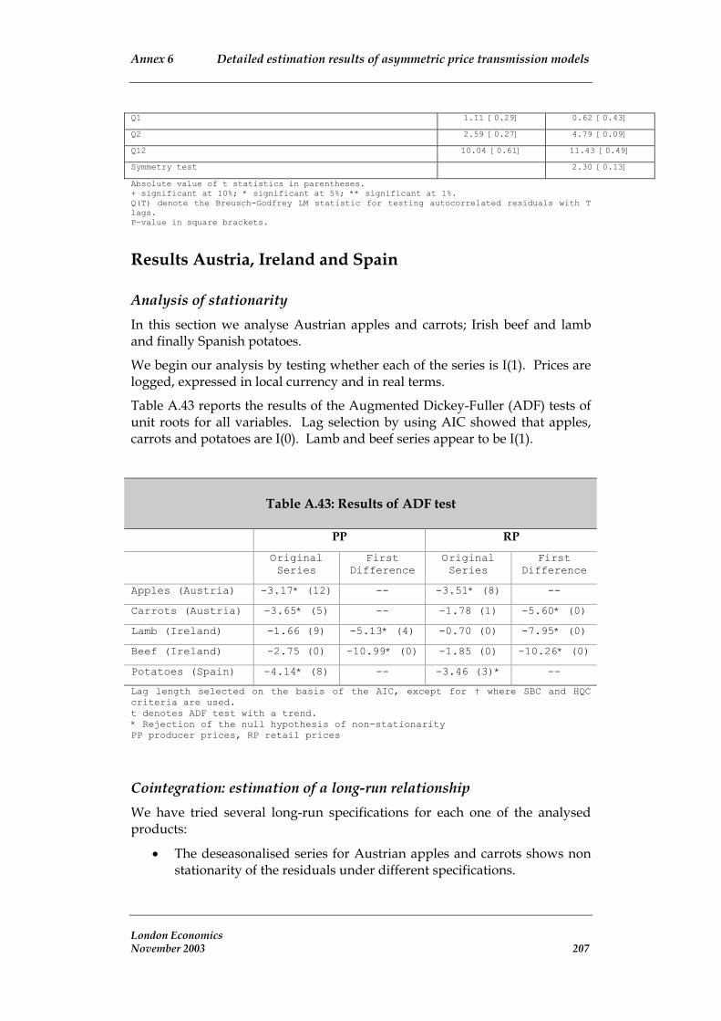
Annex 6 Detailed estimation results of asymmetric price transmission models
Q1 1.11 [0.29] 0.62 [0.43]
Q2 2.59 [0.27] 4.79 [0.09]
Q12 10.04 [0.61] 11.43 [0.49]
2.30 [0.13] Symmetry test
Absolute value of t statistics in parentheses. + significant at 10%; * significant at 5%; ** significant at 1%. Q(T) denote the Breusch-Godfrey LM statistic for testing autocorrelated residuals with T lags. P-value in square brackets.
Results Austria, Ireland and Spain
Analysis of stationarity In this section we analyse Austrian apples and carrots; Irish beef and lamb and finally Spanish potatoes.
We begin our analysis by testing whether each of the series is I(1). Prices are logged, expressed in local currency and in real terms.
Table A.43 reports the results of the Augmented Dickey-Fuller (ADF) tests of unit roots for all variables. Lag selection by using AIC showed that apples, carrots and potatoes are I(0). Lamb and beef series appear to be I(1).
Table A.43: Results of ADF test
PP RP
Original Series
First Difference
First Difference
Original Series
Apples (Austria) -3.17* (12) -- -3.51* (8) --
Carrots (Austria) -3.65* (5) -- -1.78 (1) -5.60* (0)
Lamb (Ireland) -1.66 (9) -5.13* (4) -0.70 (0) -7.95* (0)
-2.75 (0) -10.99* (0) -10.26* (0)
-4.14* (8) -- --
Beef (Ireland) -1.85 (0)
Potatoes (Spain) -3.46 (3)*
Lag length selected on the basis of the AIC, except for † where SBC and HQC criteria are used.
PP producer prices, RP retail prices
We have tried several long-run specifications for each one of the analysed products:
t denotes ADF test with a trend. * Rejection of the null hypothesis of non-stationarity
Cointegration: estimation of a long-run relationship
• The deseasonalised series for Austrian apples and carrots shows non stationarity of the residuals under different specifications.
London Economics November 2003 207

Annex 6 Detailed estimation results of asymmetric price transmission models
• The deseasonalised series for Irish beef long-run relationship shows non-stationarity of the residuals. The long-run relationship between farm and consumer lamb prices shows contradictory results: the retail prices equation (i.e. retail prices dependent on producer prices) showed non-stationarity of the residuals under different specifications. In contrast, the residuals from the producer prices equation (i.e. producer prices dependent on retail prices) showed stationarity of the residuals. For this reason we have not analysed the price series of Irish lamb.
• The long-run regressions for Spanish potatoes showed stationarity of the residuals after inclusion of a trend.
Table A.44: Retail-producer long-run equations.
Chain analysed Long-run equation ADF1 test for
stationarity of û1t (lags)
Sample period
Apples(d) PRt =2.84+0.12PPt + u1t -2.93 (6) 1997m1-2001m12
PRt =2.39+0.15PPt + u1t -1.71 (0)
Lamb(d) PRt = 1.08+0.45PPt+ u1t -2.46 (3) 1997m1-2002m3
Beef(d) PRt = 1.49+0.08PPt+ u1t -2.68 (3) 1997m1-2002m3
Potatoes(d) PRt = 2.90+0.39PPt+0.00TREND+ u1t -3.89* (12) 1985m1-2001m12
Carrots(d) 1997m1-2001m12
1 Model chosen on the basis of AIC criterion. 2 Deseasonalised series are indicated by (d). * Residuals stationary (rejection of null hypothesis of no stationarity at 95% level).
The results for the producer-retail long-run relationship are presented in Table A.45, and show cointegration results similar to those in the previous table. One exception is the equation for apples, where a trend was needed to make the residuals stationary.
London Economics November 2003 208

Annex 6 Detailed estimation results of asymmetric price transmission models
Table A.45: Producer-retail long-run equations.
Chain analysed Long-run equation ADF1 test for
stationarity of û1t (lags)
Sample period
Apples(d) PPt =-5.49+2.27PRt + u1t -3.37 (0) 1997m1-2001m12
Carrots(d) PPt =2.92+1.52PRt + u1t -3.37 (5) 1997m1-2001m12
Lamb(d) PPt = -1.28+1.49PRt+ u1t -5.08* (3) 1997m1-2002m3
Beef(d) PPt =-1.80+1.56PRt+ u1t -0.93 (0) 1997m1-2002m3
Potatoes(d) PPt = -4.97+1.99PRt-0.00TREND+ u1t -3.97* (12) 1985m1-2001m12
1 Model chosen on the basis of AIC criterion. 2 Deseasonalised series are indicated by (d). * Residuals stationary (rejection of null hypothesis of no stationarity at 95% level).
In the next paragraphs we present the results of the error correction models for the retail and producer price models. For purposes of comparison, estimates of both asymmetric and symmetric error correction models are presented, for the models for retail prices and for the producer prices.
Austrian Apples The series for retail and producer prices are I(0) but there is no long-run relationship between deseasonalised Austrian retail and farm apple prices. We have proceeded to estimate the models in first differences but without inclusion of the error correction term. In a further step we have tested for Granger-causality.
The equation of consumer prices shows Granger-causality from producer prices. Differences for increases in producers are statistically significant but not different from each other (F in the symmetry test is 1.67 with p-value 0.20). Thus the hypothesis of symmetry cannot be rejected.
Producer prices seem to be Granger-caused by retail prices but increases and decreases in retail prices are not statistically different from zero.
Estimates of the models for Apples (retail prices) RP APPLES Symmetric Asymmetric
∆RPt-1 -0.44 (3.48)** -0.36 (2.69)*
∆RPt-2 0.03 (0.28) 0.09 (0.75)
London Economics November 2003 209

Annex 6 Detailed estimation results of asymmetric price transmission models
∆RPt-3 -0.09 (0.79) -0.09 (0.75)
∆RPt-4 -0.29 (2.71)** -0.30 (2.83)**
∆RPt-5 0.11 (0.96) 0.13 (1.13)
∆RPt-6 0.43 (3.59)** 0.45 (3.78)**
∆RPt-7 -0.02 (0.13) -0.02 (0.18)
∆PPt 0.06 (2.38)*
∆PPt-1 0.07 (3.06)**
∆+PPt -0.00 (0.05)
∆+PPt-1 0.12 (2.95)**
∆-PPt 0.08 (2.34)*
∆-PPt-1 0.01 (0.20)
Constant 0.00 (0.97) 0.00 (0.16)
Observations 52 52
R-squared 0.61 0.64
Test Granger 6.92 [0.00]
Q1 2.23 [0.14] 3.00 [0.08]
Q2 3.42 [0.18] 4.57 [0.10]
Q12 12.79 [0.38] 14.28 [0.28]
F test positives 4.43 [0.02]
F test negatives 3.03 [0.06]
Symmetry test 1.67 [0.20]
Absolute value of t statistics in parentheses. + significant at 10%; * significant at 5%; ** significant at 1%. Q(T) denote the Breusch-Godfrey LM statistic for testing autocorrelated residuals with T lags. P-value in square brackets.
Estimates of the models for Apples (producer prices) PP APPLES Symmetric Asymmetric
∆PPt-1 -0.13 (0.94) -0.13 (0.87)
∆PPt-2 -0.13 (0.93) -0.12 (0.85)
∆RPt 1.55 (2.33)*
∆RPt-1 1.26 (1.88)+
∆+RPt 1.16 (1.05)
∆+RPt-1 2.05 (1.86)+
∆-RPt 1.94 (1.39)
∆-RPt-1 0.19 (0.14)
Constant 0.00 (0.00) -0.01 (0.30)
Observations 57 57
R-squared 0.13 0.15
Test Granger 3.36 [0.04]
Q1 0.65 [0.42] 0.05 [0.82]
Q2 0.83 [0.66] 0.36 [0.83]
Q12 19.18 [0.08] 17.40 [0.14]
F test positives 2.00 [0.15]
F test negatives 1.00 [0.38]
Symmetry test 0.54 [0.56]
Absolute value of t statistics in parentheses. + significant at 10%; * significant at 5%; ** significant at 1%.
London Economics November 2003 210

Annex 6 Detailed estimation results of asymmetric price transmission models
Q(T) denote the Breusch-Godfrey LM statistic for testing autocorrelated residuals with T lags. P-value in square brackets.
Austrian Carrots The series for retail and producer prices are I(0) and there is no long-run relationship between retail and farm Austrian carrots deseasonalised prices. We have proceeded to estimate the models in first differences but without inclusion of the error correction term. In a further step we have tested for Granger-causality.
The equation of consumer prices shows Granger-causality from producer prices. The equation for producer prices shows causality from consumer prices. Differences for decreases and decreases are not statistically significant for both retail or producer equations.
Estimates of the models for Carrots (retail prices) RP CARROTS Symmetric Asymmetric
RPt-1 0.02 (0.14) -0.03 (0.18)
RPt-2 -0.04 (0.31) -0.09 (0.70)
RPt-3 -0.22 (1.70)+ -0.24 (1.88)+
RPt-4 -0.05 (0.38) -0.05 (0.38)
RPt-5 0.19 (1.63) 0.20 (1.69)
RPt-6 -0.15 (1.28) -0.16 (1.31)
RPt-7 0.25 (2.00)+ 0.26 (1.99)+
RPt-8 0.26 (1.77)+ 0.33 (2.18)*
∆PPt 0.12 (3.05)**
∆PPt-1 0.05 (1.22)
∆PPt-2 0.03 (0.74)
∆PPt-3 0.08 (2.18)*
∆+PPt 0.12 (1.73)+
∆+PPt-1 0.02 (0.33)
∆+PPt-2 0.04 (0.63)
∆+PPt-3 -0.03 (0.46)
∆-PPt 0.13 (2.11)*
∆-PPt-1 0.10 (1.64)
∆-PPt-2 0.06 (0.92)
∆-PPt-3 0.20 (3.14)**
Constant -0.00 (0.29) 0.02 (1.50)
Observations 51 51
R-squared 0.39 0.48
Test Granger 3.56 [0.01]
pvG1
Q1 1.00 [0.32] 0.05 [0.82]
Q2 0.95 [0.62] 0.06 [0.97]
Q12 9.90 [0.62] 14.44 [0.27]
F test positives 1.05 [0.39]
London Economics November 2003 211

Annex 6 Detailed estimation results of asymmetric price transmission models
F test negatives 3.91 [0.01]
Symmetry test 1.45 [0.24]
Absolute value of t statistics in parentheses. + significant at 10%; * significant at 5%; ** significant at 1%. Q(T) denote the Breusch-Godfrey LM statistic for testing autocorrelated residuals with T lags. P-value in square brackets.
Estimates of the models for Carrots (producer prices) PP CARROTS Symmetric Asymmetric
∆PPt-1 -0.03 (0.17) -0.00 (0.01)
∆PPt-2 0.23 (1.62) 0.22 (1.55)
∆PPt-3 -0.26 (1.93)+ -0.33 (2.42)*
∆PPt-4 0.13 (0.96) 0.12 (0.88)
∆PPt-5 0.25 (1.87)+ 0.24 (1.80)+
∆PPt-6 -0.20 (1.53) -0.21 (1.57)
∆PPt-7 -0.30 (2.25)* -0.31 (2.24)*
∆RPt 1.25 (2.73)**
∆RPt-1 0.67 (1.44)
∆RPt-2 -0.27 (0.60)
∆RPt-3 -0.56 (1.24)
∆+RPt 0.56 (0.70)
∆+RPt-1 0.56 (0.71)
∆+RPt-2 0.13 (0.17)
∆+RPt-3 -1.68 (2.31)*
∆-RPt 1.95 (2.30)*
∆-RPt-1 0.81 (0.94)
∆-RPt-2 -0.47 (0.53)
∆-RPt-3 0.95 (1.08)
Constant 0.00 (0.26) 0.07 (1.26)
Observations 52 52
R-squared 0.42 0.49
Test Granger 3.17 [0.02]
Q1 0.02 [0.88] 0.47 [0.49]
0.18 [0.91] 1.92 [0.38]
Q12 17.07 [0.15] 21.41 [0.04]
F test positives 1.59 [0.20]
F test negatives 1.88 [0.14]
Symmetry test 1.30 [0.29]
Q2
Absolute value of t statistics in parentheses. + significant at 10%; * significant at 5%; ** significant at 1%. Q(T) denote the Breusch-Godfrey LM statistic for testing autocorrelated residuals with T lags. P-value in square brackets.
Irish Beef The equation for consumer prices shows no Granger-causality from producer prices. Moreover there are no differences when allowing different parameters for increases and decreases (F tests 0.16 and 0.02 for increases and decreases, respectively). London Economics November 2003 212

Annex 6 Detailed estimation results of asymmetric price transmission models
The same results can be reported from the equation for producer prices: no Granger-causality from consumer prices (F test 0.03) and no differences between increases and decreases.
Estimates of the models for Beef (consumer prices) RP BEEF Symmetric Asymmetric
∆RPt-1 -0.27 (2.14)* -0.27 (2.12)*
∆PPt -0.01 (0.23)
∆+PPt -0.06 (0.39)
∆-PPt 0.01 (0.13)
-0.00 (0.50) -0.00 (0.03)
Observations 61 61
R-squared 0.07 0.08
Test Granger 0.05 [0.82]
Q1 0.13 [0.71] 0.10 [0.75]
Q2 2.35 [0.31] 1.83 [0.40]
Q12 11.69 [0.47] 11.40 [0.49]
F test positives 0.16 [0.69]
F test negatives 0.02 [0.89]
0.11 [0.74]
Constant
Symmetry test
Absolute value of t statistics in parentheses. + significant at 10%; * significant at 5%; ** significant at 1%. Q(T) denote the Breusch-Godfrey LM statistic for testing autocorrelated residuals with T lags. P-value in square brackets.
Estimates of the models for Beef (producer prices) Symmetric Asymmetric
(0.17)
0.04 (0.08)
∆-RPt -0.14 (0.25)
Constant -0.00 (1.52) -0.01 (1.04)
Observations 62 62
R-squared 0.00 0.00
Test Granger 0.03 [0.87]
Q1 0.18 [0.67] 0.22 [0.64]
Q2 0.26 [0.88 0.33 [0.85]
Q12 12.56 [0.40] 14.64 [0.26]
F test negatives 0.06 [0.80]
Symmetry test 0.04 [0.84]
PP BEEF
∆RPt -0.04
∆+RPt
F test positives 0.01 [0.93]
Absolute value of t statistics in parentheses. + significant at 10%; * significant at 5%; ** significant at 1%. Q(T) denote the Breusch-Godfrey LM statistic for testing autocorrelated residuals with T lags. P-value in square brackets.
Spanish Potatoes We have estimated an error correction model for the potatoes prices. Although the series were originally found to be I(0) a very high number of the London Economics November 2003 213

Annex 6 Detailed estimation results of asymmetric price transmission models
models estimated showed autocorrelation. The problem was solved when we used the series in first differences and estimated the error correction model.
The t-statistics for ECTt-1 in the column for retail price indicate that retail prices respond to shocks that make the relationship deviate from the long-run equilibrium. There is symmetric price adjustment because, ECT+t-1 is not significanty different from ECT-t-1.
The t-statistics for ECTt-1 in the column for farm price indicate that farm prices respon to shocks that make the relationship deviate from the long-run equilibrium. Retail prices asymmetric adjustment is rejected because, although both ECT+t-1 and ECT-t-1 are individually statistically different from zero, the F test for equality of both parameters cannot be rejected (F value is 0.18 with a p-value of 0.67).
Estimates of the models for Potatoes (retail prices) RP POTATOES Symmetric Asymmetric
∆RPt-1 0.25 (2.50)* 0.23 (2.31)*
-0.21 (2.23)* -0.22 (2.33)*
∆RPt-3 -0.05 (0.60) -0.07 (0.77)
∆RPt-4 0.01 (0.12) 0.00 (0.03)
∆RPt-5 0.04 (0.49) 0.03 (0.32)
∆RPt-6 0.00 (0.02) -0.01 (0.07)
∆RPt-7 0.08 (0.98) 0.08 (0.91)
∆RPt-8 0.03 (0.42) 0.02 (0.28)
∆RPt-9 0.12 (1.51) 0.11 (1.31)
∆RPt-10 -0.09 (1.16) -0.10 (1.32)
∆RPt-11 0.22 (3.10)** 0.20 (2.63)**
∆RPt-12 0.21 (3.42)** 0.20 (3.16)**
∆PP 0.23 (10.82)** 0.22 (10.49)**
∆PP-1 0.05 (1.27) 0.06 (1.43)
∆PP-2 0.01 (0.33) 0.02 (0.45)
∆PP-3 0.05 (1.30) 0.06 (1.46)
∆PP-4 -0.00 (0.11) 0.00 (0.12)
∆PP-5 -0.01 (0.36) -0.01 (0.21)
∆PP-6 0.00 (0.13) 0.01 (0.34)
∆PP-7 -0.02 (0.50) -0.01 (0.30)
∆PP-8 -0.03 (0.79) -0.02 (0.68)
∆PP-9 -0.04 (1.28) -0.03 (1.03)
∆PP-10 0.02 (0.66) 0.02 (0.78)
∆PP-11 -0.01 (0.43) -0.00 (0.06)
-0.10 (3.48)**
ECTt-1 -0.23 (3.02)**
-0.32 (3.08)**
ECT-t-1 -0.14 (1.29)
Constant 0.00 (0.15) 0.01 (1.14)
Observations 184 184
∆RPt-2
∆PP-12 -0.09 (3.09)**
ECT+t-1
London Economics November 2003 214

Annex 6 Detailed estimation results of asymmetric price transmission models
R-squared 0.70 0.71
Test Granger 16.36 15.42
Test Granger 16.36 [0.00] 15.42 [0.00]
Q1 1.00 [0.32] 1.46 [0.23]
Q2 1.73 [0.42] 2.55 [0.28]
Q12 13.07 [0.36] 12.63
1.56 [0.21] Symmetry test
Absolute value of t statistics in parentheses. + significant at 10%; * significant at 5%; ** significant at 1%. Q(T) denote the Breusch-Godfrey LM statistic for testing autocorrelated residuals with T lags. P-value in square brackets.
Estimates of the models for Potatoes (producer prices) Symmetric Asymmetric
∆PPt-1 0.11 (1.16) 0.12 (1.17)
∆PPt-2 -0.14 (1.49) -0.14 (1.47)
∆PPt-3 -0.07 (0.81) -0.07 (0.81)
∆PPt-4 0.13 (1.54) 0.13 (1.52)
∆RPt 1.84 (10.70)** 1.85 (10.65)**
∆RPt-1 -0.39 (1.69)+ -0.39 (1.70)+
∆RPt-2 0.36 (1.71)+ 0.36 (1.71)+
∆RPt-3 0.09 (0.45) 0.10 (0.49)
∆RPt-4 -0.14 (0.75) -0.14 (0.76)
∆RPt-5 -0.13 (0.81) -0.13 (0.79)
∆RPt-6 0.03 (0.20) 0.03 (0.19)
∆RPt-7 0.12 (0.73) 0.12 (0.71)
0.13 (0.77) 0.13 (0.77)
∆RPt-9 -0.12 (0.75) -0.12 (0.71)
∆RPt-10 0.16 (0.95) 0.16 (0.95)
∆RPt-11 -0.18 (1.15) -0.18 (1.12)
∆RPt-12 -0.46 (3.11)** -0.45 (3.01)**
ECTt-1 -0.24 (2.86)**
ECT+t-1 -0.20 (1.75)+
-0.28 (2.14)*
-0.01 (0.47)
0.56
Test Granger 11.21 [0.00] 10.42 [0.00]
Q1 0.58 [0.45] 0.42 [0.52]
2.09 [0.35] 1.89 [0.39]
Q12 12.76 [0.39] 12.17 [0.43]
Symmetry test 0.18 [0.67]
PP POTATOES
∆RPt-8
ECT-t-1
Constant -0.00 (0.22)
Observations 184 184
R-squared 0.56
Q2
Absolute value of t statistics in parentheses. + significant at 10%; * significant at 5%; ** significant at 1%. Q(T) denote the Breusch-Godfrey LM statistic for testing autocorrelated residuals with T lags. P-value in square brackets.
London Economics November 2003 215

Annex 7 Detailed estimation results of semi-structural models
Annex 7 Detailed estimation results of semi-structural models
Figure A.18: Red meat
Arellano-Bond dynamic panel-data estimation Number of obs = 78
F(12, 61) = 653.96
------------------------------------------------------------------------------
cshare |
lintgoodpi |
c5_9 |
c5_7 |
yy7 |
_cons | -.2198232 .1063859 -2.07 0.043 -.432555 -.0070914
H0: no autocorrelation z = -0.88 Pr > z = 0.3809
Group variable (i): fe Number of groups = 13
Time variable (t): year Obs per group: min = 6 avg = 6 max = 6 One-step results
| Robust D.spread_p | Coef. Std. Err. t P>|t| [95% Conf. Interval] -------------+---------------------------------------------------------------- spread_p | LD | .5016713 .1470188 3.41 0.001 .2076891 .7956535 L2D | -.8681911 .0750897 -11.56 0.000 -1.018342 -.7180401
D1 | 12.29151 5.260315 2.34 0.023 1.772856 22.81015 scare_b | D1 | .3628074 .1239768 2.93 0.005 .1149004 .6107144
D1 | 5.524375 2.378299 2.32 0.024 .7686723 10.28008 uk_eu | D1 | -3.006008 1.106223 -2.72 0.009 -5.218038 -.7939777
D1 | .0182585 .0493072 0.37 0.712 -.0803374 .1168544 c5_3 | D1 | -.0003135 .010996 -0.03 0.977 -.0223014 .0216744 c5_4 | D1 | -.0083298 .0128648 -0.65 0.520 -.0340545 .0173949 c5_5 | D1 | -.0003939 .0148555 -0.03 0.979 -.0300993 .0293114
D1 | .0403816 .0288344 1.40 0.166 -.0172762 .0980395 yy5 | D1 | .1934073 .1071475 1.81 0.076 -.0208473 .407662 yy6 | D1 | .7382981 .1895076 3.90 0.000 .3593543 1.117242
D1 | .9845408 .2503018 3.93 0.000 .4840314 1.48505 yy8 | D1 | .9859634 .4120065 2.39 0.020 .1621055 1.809821 yy9 | D1 | 1.553433 .4671882 3.33 0.001 .619232 2.487633
------------------------------------------------------------------------------ Arellano-Bond test that average autocovariance in residuals of order 1 is 0: H0: no autocorrelation z = -1.94 Pr > z = 0.0529 Arellano-Bond test that average autocovariance in residuals of order 2 is 0:
Source: LE estimates
London Economics November 2003 216

Annex 7 Detailed estimation results of semi-structural models
Figure A.19: Wheat products
Arellano-Bond dynamic panel-data estimation Number of obs = 49 Group variable (i): fe Number of groups = 11 F(10, 25) = 511.77 Time variable (t): year Obs per group: min = 2 avg = 4.454545 max = 6 One-step results ------------------------------------------------------------------------------ | Robust D.spread_p | Coef. Std. Err. t P>|t| [95% Conf. Interval] -------------+---------------------------------------------------------------- spread_p | LD | .4117274 .0698593 5.89 0.000 .2678495 .5556052 L2D | .2599763 .0238464 10.90 0.000 .2108636 .3090889 cshare | D1 | 7.403377 5.089052 1.45 0.158 -3.077723 17.88448 lintgoodpi | D1 | 27.56017 16.63502 1.66 0.110 -6.700288 61.82063 lip | D1 | 18.04565 15.0207 1.20 0.241 -12.89006 48.98136 cap_change |
D1 | 5.328366 4.514737 1.18 0.249 -3.969909 14.62664
c5_9 |
c5_8 |
trend_1 |
D1 | -2.070308 .9749331 -2.12 0.044 -4.07822 -.0623955
trend_8 |
H0: no autocorrelation z = 0.03 Pr > z = 0.9749
D1 | -2.772108 1.09838 -2.52 0.018 -5.034263 -.5099529 uk_eu | D1 | -11.6261 5.319057 -2.19 0.038 -22.5809 -.6712954 dk_eu |
nc_dollar | D1 | .6329007 .8785723 0.72 0.478 -1.176553 2.442354 nc_hdollar | D1 | -2.095928 6.650758 -0.32 0.755 -15.79342 11.60156
D1 | -.6331101 .4087394 -1.55 0.134 -1.474925 .2087043 c5_1 | D1 | -.3693207 .2093495 -1.76 0.090 -.8004841 .0618427 c5_2 | D1 | .2126687 .1762982 1.21 0.239 -.1504242 .5757617 c5_4 | D1 | -.487213 .1828098 -2.67 0.013 -.8637168 -.1107092 c5_6 | D1 | -.1661917 .0616375 -2.70 0.012 -.2931365 -.039247 c5_7 | D1 | -.3181763 .1055282 -3.02 0.006 -.5355158 -.1008368
D1 | -.0176839 .0755716 -0.23 0.817 -.1733266 .1379588 trend_c | D1 | .954286 .8225884 1.16 0.257 -.7398664 2.648438
D1 | 1.276107 .5048542 2.53 0.018 .2363406 2.315874 trend_2 |
trend_4 | D1 | 1.63442 .4637952 3.52 0.002 .6792165 2.589624 trend_7 | D1 | .5103479 .2722074 1.87 0.073 -.0502738 1.07097
D1 | .7797778 .2711927 2.88 0.008 .221246 1.33831 Arellano-Bond test that average autocovariance in residuals of order 1 is 0: H0: no autocorrelation z = -1.93 Pr > z = 0.0534 Arellano-Bond test that average autocovariance in residuals of order 2 is 0:
Source: LE estimates
London Economics November 2003 217

Annex 7 Detailed estimation results of semi-structural models
Figure A.20: Poultry
Arellano-Bond dynamic panel-data estimation Number of obs = 50 Group variable (i): fe Number of groups = 13 F(11, 25) = 698183.32
trend_c |
D1 | -.1162946 .1943256 -0.60 0.555 -.5165157 .2839265
D1 | .2068713 .2832224 0.73 0.472 -.3764361 .7901787
_cons | (dropped)
H0: no autocorrelation z = -1.65 Pr > z = 0.0988
Time variable (t): year Obs per group: min = 1 avg = 3.846154 max = 6 One-step results ------------------------------------------------------------------------------ | Robust D.spread_p | Coef. Std. Err. t P>|t| [95% Conf. Interval] -------------+---------------------------------------------------------------- spread_p | LD | .1077899 .2741067 0.39 0.697 -.4567435 .6723233 L2D | -.2031458 .1428784 -1.42 0.167 -.4974094 .0911178 cshare | D1 | 1.012569 3.159027 0.32 0.751 -5.493569 7.518708 lintgoodpi | D1 | 4.353282 5.533298 0.79 0.439 -7.042758 15.74932
D1 | -9.089642 2.323404 -3.91 0.001 -13.87478 -4.304501 c5_9 | D1 | -.1539115 .1363333 -1.13 0.270 -.4346951 .1268721
D1 | -.5077828 .146159 -3.47 0.002 -.8088028 -.2067627 c5_3 | D1 | .057001 .0440595 1.29 0.208 -.0337411 .1477432
D1 | -.0458916 .0632979 -0.73 0.475 -.1762561 .0844729 c5_5 | D1 | .0257061 .0316846 0.81 0.425 -.0395495 .0909617
D1 | -.0339708 .0498001 -0.68 0.501 -.136536 .0685944 c5_7 | D1 | .0396727 .0693285 0.57 0.572 -.1031121 .1824575
D1 | -.0476568 .0448104 -1.06 0.298 -.1399456 .0446319
D1 | .2227937 .2169414 1.03 0.314 -.2240055 .669593
D1 | -.372427 .1831917 -2.03 0.053 -.7497175 .0048634 trend_4 | D1 | -.0368844 .1827186 -0.20 0.842 -.4132005 .3394316
D1 | -.2198976 .2215856 -0.99 0.331 -.6762617 .2364665 trend_7 |
D1 | -.3962504 .3556569 -1.11 0.276 -1.128739 .3362386 yy5 | D1 | .019236 .1306047 0.15 0.884 -.2497494 .2882214
yy7 | D1 | .5905218 .5493838 1.07 0.293 -.5409553 1.721999
D1 | -.0069139 .1821534 -0.04 0.970 -.3820658 .368238
------------------------------------------------------------------------------
H0: no autocorrelation z = -2.34 Pr > z = 0.0192 Arellano-Bond test that average autocovariance in residuals of order 2 is 0:
uk_eu |
c5_2 |
c5_4 |
c5_6 |
c5_8 |
trend_3 |
trend_5 |
trend_8 |
yy6 |
yy8 |
Arellano-Bond test that average autocovariance in residuals of order 1 is 0:
Source: LE estimates
London Economics November 2003 218
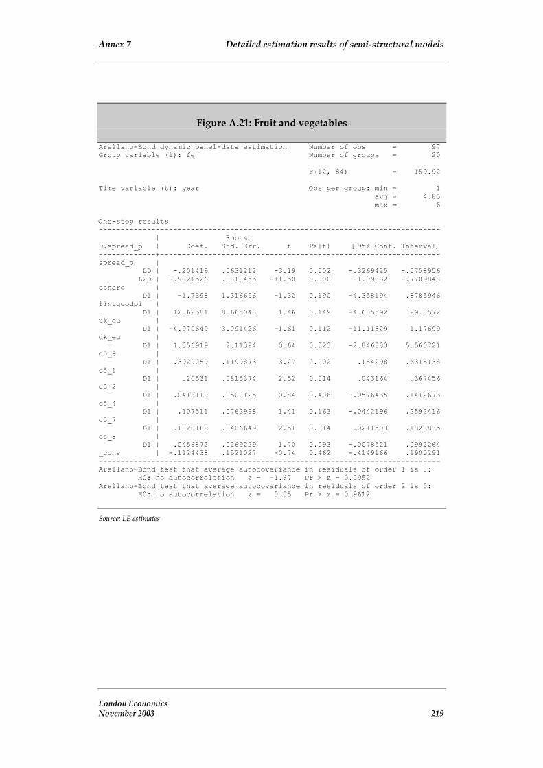
Annex 7 Detailed estimation results of semi-structural models
Figure A.21: Fruit and vegetables
Arellano-Bond dynamic panel-data estimation Number of obs = 97 Group variable (i): fe Number of groups = 20
F(12, 84) = 159.92
Time variable (t): year Obs per group: min = 1
max = 6
D.spread_p | Coef. Std. Err. t P>|t| [95% Conf. Interval]
cshare |
c5_9 |
avg = 4.85
One-step results ------------------------------------------------------------------------------ | Robust
-------------+---------------------------------------------------------------- spread_p | LD | -.201419 .0631212 -3.19 0.002 -.3269425 -.0758956 L2D | -.9321526 .0810455 -11.50 0.000 -1.09332 -.7709848
D1 | -1.7398 1.316696 -1.32 0.190 -4.358194 .8785946 lintgoodpi | D1 | 12.62581 8.665048 1.46 0.149 -4.605592 29.8572 uk_eu | D1 | -4.970649 3.091426 -1.61 0.112 -11.11829 1.17699 dk_eu | D1 | 1.356919 2.11394 0.64 0.523 -2.846883 5.560721
D1 | .3929059 .1199873 3.27 0.002 .154298 .6315138 c5_1 | D1 | .20531 .0815374 2.52 0.014 .043164 .367456 c5_2 | D1 | .0418119 .0500125 0.84 0.406 -.0576435 .1412673 c5_4 | D1 | .107511 .0762998 1.41 0.163 -.0442196 .2592416 c5_7 | D1 | .1020169 .0406649 2.51 0.014 .0211503 .1828835 c5_8 | D1 | .0456872 .0269229 1.70 0.093 -.0078521 .0992264 _cons | -.1124438 .1521027 -0.74 0.462 -.4149166 .1900291 ------------------------------------------------------------------------------ Arellano-Bond test that average autocovariance in residuals of order 1 is 0: H0: no autocorrelation z = -1.67 Pr > z = 0.0952 Arellano-Bond test that average autocovariance in residuals of order 2 is 0: H0: no autocorrelation z = 0.05 Pr > z = 0.9612
Source: LE estimates
London Economics November 2003 219
Annex 8Estimation results for dairy products: Causal links between retail prices of dairy products and farm gate prices
Annex 8 Estimation results for dairy products: Causal links between retail prices of dairy products and farm gate prices40
Background In this section we investigate the relationship between farm gate and retail prices for milk and dairy products. It may seem quite natural to assume that retail prices depend on what is charged at the farm gate. After all, retail price should include the farm price plus wholesale and retail costs, plus any margins earned at each level. However, if we think about changes in the price, the direction of causality may be reversed. For example, a demand shock —that starts with the consumer buying less milk— hits the retailers first, forcing them to lower their own prices. Retailers might be able to pass this on back along the chain. In this case, a change in the retail price would help to explain why there has been a change in the farm gate price and not vice versa41.
Price transmission exists when fluctuations in farm gate prices are passed on at the retail level, or vice versa. Using data on farm gate and retail prices for milk and dairy products we investigate econometrically whether there exists any evidence of price transmission in the dairy supply chain and whether this transmission is different for positive and negative price shocks.
The object of price transmission analysis is to provide answers to the following questions: by how much is a change in the farm price reflected in the retail price and vice versa? Is there a difference in the way that the retail price adjusts to an increase or a decrease in farm price and vice versa?
The nature of the transmission of price changes along the dairy chain varies substantially across the four countries that we studied in detail, namely the UK, Denmark, France and Germany. Some of the differences could be attributed to a different market structure, differences in the transmission of information, or government intervention. The absence of statistically significant price transmission implies that prices at the upstream and downstream ends of the milk chain are independent of each other. In other words, prices at each end are fully insulated from developments and shocks at the other end of the chain.
40 With permission from the Milk Development Council.
41 There are multiple stages in the supply chain. These include transport, processing, storage and distribution. Our exercise investigates the relationship between initial prices at farm gate and final prices at retail. However, there could be significant forces at each of these stages that also affect price transmission.
London Economics November 2003 220

Annex 8Estimation results for dairy products: Causal links between retail prices of dairy products and farm gate prices
We start by testing for price transmission in the UK. We then perform similar tests for major milk markets in the EU, namely France, Germany and Denmark. This will enable to examine whether there are any differences across these markets.
Data sources The data required for the analysis consists of series of prices at farm gate and retail for the EU countries under consideration.
Data on farm gate prices has been obtained from Eurostat for all the European countries except for Denmark, where the data was provided by Statistics Denmark. To make the price series comparable with retail prices and among countries we have constructed index numbers (1995=100) from the prices expressed at the local currency. Farm gate prices from the Netherlands are missing for the whole year 1999. Therefore, the subsequent analysis cannot be undertaken for Netherlands.
Data series of retail dairy prices are provided by the respective national statistical agencies of each European country. The data that are available are the following:
• For the UK, retail price indices are provided only for pasteurised milk, cheddar cheese and home-produced butter. This limited the choice of dairy products to be included in the study to three group categories, namely liquid milk, cheese and butter.
• For Germany and Denmark, consumer dairy price indices are available at a more disaggregated level. We chose the most representative products of the categories of liquid milk, cheese and butter (see Table A.46).
• In France, retail prices are currently being provided for the products milk and cream, cheeses, and yoghurts and dairy deserts. However, in previous years the consumer prices were provided at a more disaggregated level. We aggregated data of previous years to last year’s three categories using the weights from the consumer price index.
The frequency of the data is monthly. Our sample is constituted of prices from January 1995 to December 2001. The list of all variables and their names are listed in Table A.46, together with their sources. The product categories used in our analysis are liquid milk, cheese and butter for UK, Germany and Denmark; and liquid milk, cheese and yoghurt for France.
London Economics November 2003 221

Annex 8Estimation results for dairy products: Causal links between retail prices of dairy products and farm gate prices
Table A.46: Sources of data
Country Name Variable Source UK Raw milk Raw cows’ milk; 3.7% fat content Eurostat
Milk Milk, pasteurised ONS
Cheese Cheddar Cheese
ONS
Butter Butter, Home Produced ONS
Germany Raw milk Raw cows’ milk; 3.7% fat content Eurostat
Milk Whole milk Federal Statistics Office
Cheese German Emmentaler cheese
Federal Statistics Office
Butter Butter Federal Statistics Office
Denmark Raw milk Whole milk 4,20 pct. Fat and 3,40 pct. Protein Statistics Denmark
Milk Whole milk / full-cream milk Statistics Denmark
Cheese Cheese, 45% Statistics Denmark
Butter Butter Statistics Denmark
France Raw milk Raw cows’ milk; 3.7% fat content Eurostat
Milk Milk and Cream INSEE
Cheese Cheeses INSEE
Yoghurt Yoghurts and Dairy Deserts INSEE
Netherlands Not used Raw cows’ milk; 3.7% fat content Eurostat
Not used Milk Central Bureau of Statistics
Not used Cheese Central Bureau of Statistics
Not used Butter Central Bureau of Statistics
Methodological issues in the estimation of price transmission
Econometric specification We use vector autoregressions (VARs) to identify causation between time series of farm gate and retail prices. Although VAR interpretation in terms of causal relationship is rather controversial they represent a widely used instrument of analysis for identifying relationships among variables. Since the main interest of our analysis is to identify possible links among variables, VAR methodology seems well-suited as little a priori knowledge is imposed.
A characteristic of the dairy processing industry is that inputs (raw milk at farm gate) can be transformed in more than one final product (whole milk, cheese, butter, yoghurt, etc). Therefore we will also investigate the links
London Economics November 2003 222

Annex 8Estimation results for dairy products: Causal links between retail prices of dairy products and farm gate prices
between the price of raw milk and the price of a number of products other than milk.
An advantage of VAR is that it can treat more than one endogenous variable in the system. It can allow each variable to affect all the other variables as well as being affected by them. It is therefore possible to explore the existence of feedback effects, and reverse causality, running in from retail to farm gate.
To test for the existence of causality, for each country of interest, we apply Granger-causality tests to various pairs of series of farm gate and retail price series. Granger-causality tests provide a statistical measure of the extent to which lagged values of one variable are important in the prediction of another variable, once lagged values of the latter are also included in the model42. It is important to note that the Granger test does not by itself measure causality in the more common use of the term, but it provides a measure of how much of the information in y can be explained by previous values of x.
We use Granger-causality tests to test whether upstream prices cause downstream prices, and/or vice versa.
Granger-causality tests may give misleading results if the variables in the VAR contain unit roots43. In such a case, one must use either VAR models in first differences or cointegration VAR models if the underlying variables are cointegrated. Therefore, in a first stage we will assess whether the variables are stationary.
Our approach is as follows: First, we test whether all variables are non-stationary. If evidence of unit roots is found, we search for a cointegration relationship among the variables and estimate the cointegrating regression. We then proceed to test for Granger-causality with series expressed in first differences. The model includes the cointegration relationship if the variables are cointegrated.
So far we have assumed an identical response in farm gate (retail) prices to a shock in retail (farm gate) prices irrespective of whether the shock is positive or negative. In a further step we allow for asymmetric responses to shocks testing separately for the impact of price increases and decreases in the Granger-causality test.
Granger tests have been used frequently in empirical studies of price transmission. For example, Lamm and Westcott (1981) found that, for dairy products as a group, the direction of causality runs from farm to retail. For
42 In other words, a variable x is said not to Granger-cause another variable y if past values of x do not help predict the value of y. Note that the formal hypothesis in the Granger-causality test is “x does not to Granger-cause y”. However, much of the literature uses the term “Granger-causality” to refer to the test in general.
43 A variable is said to contain a unit root or is I(1) if it is non-stationary. A time series is defined stationary if its mean, variance and covariances are time invariant (constant over time).
London Economics November 2003 223

Annex 8Estimation results for dairy products: Causal links between retail prices of dairy products and farm gate prices
the two individual dairy products studied by Heien (1980), a joint causal relationship between wholesale and retail price was found for butter and a unidirectional downward relationship was found for milk.
Granger-causality test In testing the causality running from the upstream stage to the downstream stage, the Granger approach estimates first how much of the variations in the downstream price ( ) can be explained by its own past values. One then
tests whether adding lagged values of upstream price variations in ( ∆ ) can improve the explanatory power of the model. A similar, but reverse approach is taken for testing for causality running from the downstream stage to the upstream stage. Put in VAR form this means estimating for each relevant pair of prices the following equations:
DtP∆
UtP
∑∑=
−=
− +∆+∆+=∆k
jt
Djtj
k
j
Ujtj
Dt PPP
111
111 εγβα
∑∑=
−=
− +∆+∆+=∆k
jt
Djtj
k
j
Ujtj
Ut PPP
122
122 εγβα
where k are the number of lags, ∆ is the one-period growth rate operator, and t1ε and t2ε are error terms. α , β and γ denote parameters to be estimated.
UtP∆ is said to be Granger-causing if (with lags) helps in the
prediction of , or equivalently if the coefficients on the lagged are jointly statistically significant.
DtP∆ U
tP∆DtP∆ U
tP∆
Asymmetric responses in the Granger-causality test Testing asymmetry in the effects of farm gate price variations on retail prices requires conducting the Granger-causality test separately on positive and negative farm price changes. The same can be said for asymmetric deviations from retail to farm gate so that previous equations can be written as:
∑∑∑=
−=
−−−
=−
++ +∆+∆+∆+=∆k
jt
Djtj
k
j
Ujtj
k
j
Ujtj
Dt PPPP
111
11
111 εγββα
t
k
j
Djtj
k
j
Djtj
k
j
Ujtj
Ut PPPP 2
12
12
122 εγγβα +∆+∆+∆+=∆ ∑∑∑
=−
−−
=−
++
=−
where is the increase in the upstream price at period t with its
corresponding parameter, and would be a decrease in the
Utj P++ ∆1β
Utj P−− ∆1β
London Economics November 2003 224

Annex 8Estimation results for dairy products: Causal links between retail prices of dairy products and farm gate prices
upstream price at period t with its corresponding parameter. The same applies for increases and decreases in the downstream price.
The null hypothesis that does not Granger-cause ∆ is tested
using the Wald statistic for the joint hypothesis: .
Utj P++ ∆1β D
tP
1= +kβ 0...1211 === ++ ββ
Analysis of non-stationarity A necessary condition for Granger-causality tests is that each of the time series is stationary. If the series are integrated of order one, I(1), the test should be performed on differenced series. In addition if series are I(1), the potential use of cointegration is to be tested by examining the possibility of the existence of a long-run relationship.
The estimation begins with an Augmented Dickey-Fuller (ADF) test of unit roots in all variables. Our first finding is that prices of cheese in Denmark are stationary. The rest of variables are I(1) (see Table A9.1) except for price of raw milk in UK and France, and price of cheese in Germany, whose first differences are non-stationary.
Since the prices of raw milk show a seasonal pattern for UK, Germany and France, we proceed to filter the series44 (Enders, 1995) and test for unit roots on the deseasonalised time series. The results of the test show that filtered series are I(1) and their first difference stationary (see Table A9.2). This implies that the original series contain a unit root and deterministic seasonality.
In the analysis we use the deseasonalised series for prices of raw milk in the UK, Germany and France. Since the variable for cheese in Denmark has a different order of integration than the rest of variables we exclude it in the analysis. Finally, the price of cheese in Germany in first differences is not stationary at a 5% level, hence we will put less weight on the results related to the price of cheese in Germany.
44 The deseasonalised-filtered series is the series of estimated residuals from a regression that contains only seasonal dummy variables.
London Economics November 2003 225

Annex 8Estimation results for dairy products: Causal links between retail prices of dairy products and farm gate prices
Table A9.1: Augmented Dickey-Fuller tests
Country Variable ADF
(levels) ADF (first difference)
UK Raw cows’ milk; 3.7% fat content -2.1043 (12) rt -1.3078 (11) rt
Milk, pasteurised -0.97515 (0) rt -9.8481 (0)
Cheddar Cheese
-1.6367 (0) rt -8.4032 (0)
Butter, Home Produced -0.43987 (0) rt -9.0945 (0)
Germany Raw cows’ milk; 3.7% fat content -2.6205 (12) r -5.9312 (4)
Whole milk -1.1164 (1) rt -4.267 (0)
German Emmentaler cheese -1.0434 (2) rt -1.9031 (1) rt
Butter -2.304 (1) rt -3.4009 (0) t
Denmark Whole milk 4,20 pct. Fat and 3,40 pct. Protein -1.0845 (0) rt -8.0808 (0)
Whole milk / full-cream milk -0.76506 (0) rt -9.7071 (0)
Cheese, 45% -3.508 (0) --
Butter -0.9677 (0) rt -8.8641 (0)
France Raw cows’ milk; 3.7% fat content -2.4532 (12) rt -1.4497 (11) rt
Milk and Cream 4.5874 (0) rt -5.1199 (0)
Cheeses 3.581 (0) rt -6.0745 (0)
Yoghurts and Dairy Deserts 1.4176 (1) rt -5.345 (0)
95% critical value for ADF -2.9023 -2.9029
Note: in brackets number of significant lags chosen with Schwarz Bayesian criterion, r indicates presence of a unit root (5% significance level), t denotes a significant time trend.
Table A9.2: Augmented Dickey-Fuller Tests on Deseasonalised Series
Country Variable ADF (levels) ADF (first difference)
UK Raw cows’ milk; 3.7% fat content -1.6673 (0) rt -8.6274 (0)
Germany Raw cows’ milk; 3.7% fat content -0.90937 (1) t -4.4821 (0)
France Raw cows’ milk; 3.7% fat content -0.9488 (0) rt -8.9462 (0)
95% critical value for ADF
-2.9023 -2.9029
Note: in brackets number of significant lags chosen with Schwarz Bayesian criterion, r indicates presence of a unit root (5% significance level), t denotes a significant time trend.
London Economics November 2003 226

Annex 8Estimation results for dairy products: Causal links between retail prices of dairy products and farm gate prices
Granger-causality: Results Given the monthly frequency of the data, we started our analysis with models including 12-lags of both the upstream and downstream prices. Next, using the “general to specific procedure” we simplified the number of lags until the residuals showed no autocorrelation. The results are reported in Table A9.3 for bivariate causality tests of all possible combinations of upstream and downstream prices as endogenous variables.
A summary of our findings of the tests (10% level of significance) are the following:
• In the UK farm gate prices are causing changes in retail prices for milk and butter. Shocks in the retail market for milk are also transmitted to the farm gate price.
• In Germany the transmission is bi-directional from farm gate to retail and vice-versa.
• For France changes in prices of raw milk are transmitted to yoghurt only. There is no other evidence of reverse transmission in France.
• Finally, in Denmark we do not find evidence of causality in either direction.
Search for a long-run equilibrium relationship between retail and farm gate prices After finding that all price series were integrated of order one, we proceeded to search for a cointegrating relationship45 between farm gate prices and retail prices. The cointegration approach assumes that economic forces operate on the two variables such that they do not drift apart significantly in the long run.
We investigated long-run equilibrium relationships between upstream and downstream prices and found no evidence of cointegration46 of the series. None of the pairs of retail-farm gate prices are cointegrated and hence no long-run equilibrium relationship appears to exist over the sample period. This suggests that the series tend to diverge over time.
Since no long-run relationship can be found, we focus our analysis on variations (price increases or decreases) that take place in the short run. We must note however, that the long-run relationship tested only refers to the sample period and we cannot reject that a long-run relationship could exist for a longer period. In addition, cointegration procedures cannot conclude
45 We estimate the long-run equilibrium relationship between the series of up-stream (PUt) and down-stream (PDt) prices as PDt = α + β PUt + εt, where α and β are parameters to be estimated and εt is an error term. Two series are said to be cointegrated, or a long-run equilibrium relationship exists, if the estimated residuals are stationary.
46 i.e. non stationarity in the estimated equilibrium errors.
London Economics November 2003 227

Annex 8Estimation results for dairy products: Causal links between retail prices of dairy products and farm gate prices
that no long-run relationship exists because they might fail to model subsidiary hypotheses or other excluded factors.
Table A9.3: Pairwise Granger-causality Tests
Null Hypothesis F statistic
UK Raw milk prices does not granger cause Retail milk price (12) 1.83*
Retail milk price does not granger cause Raw milk prices (5) 2.94**
Raw milk prices does not granger cause Cheese (1) 0.09
Cheese does not granger cause Raw milk prices (11) 0.57
Raw milk prices does not granger cause Butter (12) 1.92*
Butter does not granger cause Raw milk prices (12) 0.42
Germany Raw milk prices does not granger cause Retail milk price (4) 2.21*
Retail milk price does not granger cause Raw milk prices (9) 2.06**
Raw milk prices does not granger cause Cheese (11) 2.17**
Cheese does not granger cause Raw milk prices (8) 3.14**
Raw milk prices does not granger cause Butter (12) 1.93*
Butter does not granger cause Raw milk prices (1) 3.83*
Denmark Raw milk prices does not granger cause Retail milk price (1) 0.78
Retail milk price does not granger cause Raw milk prices (1) 0.01
Raw milk prices does not granger cause Cheese -- Cheese does not granger cause Raw milk prices --
Raw milk prices does not granger cause Butter (7) 1.18
Butter does not granger cause Raw milk prices (12) 0.86
France Raw milk prices does not granger cause Retail milk price (9) 1.41 Retail milk price does not granger cause Raw milk prices (3) 0.18 Raw milk prices does not granger cause Cheese (9) 1.16 Cheese does not granger cause Raw milk prices (3) 0.04 Raw milk prices does not granger cause Yoghurt (3) 3.92** Yoghurt does not granger cause Raw milk prices (3) 1.03 Note: In parenthesis minimum number of lags that ensure white noise residuals (using Breusch-Godfrey LM test at 5%). * Rejection of null hypothesis at 10%, ** Rejection of null hypothesis at 5%.
Granger-causality with asymmetric responses: Results So far we have implicitly assumed that the price responses were symmetric. In that sense a shock at one end of the supply chain would produce the same response in absolute terms at the other end, regardless of whether the shock reflected a price increase or decrease. In this section we introduce asymmetry by testing separately positive and negative shocks in prices47.
47 Note that this approach is different from threshold autoregressive models (TAR) introduced by Enders and Granger (1998). The TAR model is designed to capture asymmetrically movements in the series of the deviations from the long-run equilibrium. Since we found no cointegration in our series we cannot
London Economics November 2003 228

Annex 8Estimation results for dairy products: Causal links between retail prices of dairy products and farm gate prices
The findings of the tests (10% level of significance) are the following (results are presented in Table A9.4):
• In the UK, decreases in farm gate price have been transmitted to milk and butter retailer prices. In addition, increases in farm gate prices have also been transmitted to retail milk prices (i.e., retail milk prices reflect increases of farm gate prices). No other evidence of asymmetries in the transmission of price shocks is found for the UK.
• The results of the test for asymmetric transmission in Germany are mixed. Negative retail milk prices have been transmitted to the farm gate price. In addition, positive shocks in farm gate prices are also transmitted to cheese retail prices.
• The main transmission channel in France is from farm gate price to retail prices. Increases in farm gate prices have been reflected in retail prices of milk, cheese and yoghurt. In addition, price reductions at the farm gate have also been passed on to retail price of cheese.
• In Denmark there is no evidence of asymmetric price transmission.
use these models. However, our approach to asymmetric responses in prices captures the effects of short-run (up to 12 lags) shocks.
London Economics November 2003 229

Annex 8Estimation results for dairy products: Causal links between retail prices of dairy products and farm gate prices
Table A9.4: Asymmetric Granger-causality tests
Null Hypothesis F statistic UK Positive (negative) change in Raw milk prices does not granger cause Retail milk price 1.82* (1.75*)
Positive (negative) change in Retail milk prices does not granger cause Raw milk prices 1.39 (1.67)
Positive (negative) change in Raw milk prices does not granger cause Cheese 0.34 (0.05)
Positive (negative) change in Cheese milk prices does not granger cause Raw milk prices 0.84 (0.34)
Positive (negative) change in Raw milk prices does not granger cause Butter 0.65 (2.22)**
Positive (negative) change in Butter milk prices does not granger cause Raw milk prices 1.51 (1.33)
Positive (negative) change in Raw milk prices does not granger cause Retail milk price 1.55 (0.54)
Positive (negative) change in Retail milk prices does not granger cause Raw milk prices 1.43 (2.20)**
Positive (negative) change in Raw milk prices does not granger cause Cheese 1.85* (0.64)
Positive (negative) change in Cheese milk prices does not granger cause Raw milk prices 1.35 (1.52)
Positive (negative) change in Raw milk prices does not granger cause Butter 1.52 (1.58)
Positive (negative) change in Butter milk prices does not granger cause Raw milk prices 1.31 (0.34)
Denmark Positive (negative) change in Raw milk prices does not granger cause Retail milk price 0.01 (2.16)
Positive (negative) change in Retail milk prices does not granger cause Raw milk prices 0.02 (0.01)
Positive (negative) change in Raw milk prices does not granger cause Cheese --
Positive (negative) change in Cheese milk prices does not granger cause Raw milk prices --
Positive (negative) change in Raw milk prices does not granger cause Butter 1.58 (0.35)
Positive (negative) change in Butter milk prices does not granger cause Raw milk prices 0.74 (0.52)
France Positive (negative) change in Raw milk prices does not granger cause Retail milk price 2.48** (0.59)
Positive (negative) change in Retail milk prices does not granger cause Raw milk prices 1.19 (1.46)
Positive (negative) change in Raw milk prices does not granger cause Cheese 2.59** (1.80)*
Positive (negative) change in Cheese milk prices does not granger cause Raw milk prices 1.23 (1.62)
Positive (negative) change in Raw milk prices does not granger cause Yoghurt 5.01** (0.68)
Positive (negative) change in Yoghurt milk prices does not granger cause Raw milk prices 1.17 (1.16)
Note: * Rejection of null hypothesis at 10%, ** Rejection of null hypothesis at 5%.
Germany
London Economics November 2003 230

Annex 8Estimation results for dairy products: Causal links between retail prices of dairy products and farm gate prices
Results The response of retail prices to changes in farm gate prices is generally not instantaneous but delayed. The statistical tests we use provide an estimate of the extent to which lagged values of one price variable contribute to predict changes in another price variable, once lagged values of the latter are also included in the model.
In a further step we examine whether there exist any asymmetries in the price transmission, i.e. we test whether the transmission of price increases differs from the transmission of price decreases.
In Table 8.9 we summarise the findings of our empirical analysis of price transmission in the four countries (see Annex 9 for detailed estimation results). The first four columns of the table list the country, the dairy product under consideration and the prices used as explanatory variables. The fifth column reports the number of lags used for each of the models48. The last three columns show the total sum effect of all the lags of the explanatory variable on the dependent variable. The sixth column reports the estimated effect on the dependent variable in the case where price increases and decreases at one end of the chain have identical effects on the price at the other end of the chain, and the last two columns report the different effect on the price at one end of the chain of price increases and decreases at the other end of the chain, if such differences were found to be statistically significant. In addition the table reports the test statistic of the joint significance (F statistic) of the explanatory variables in parenthesis.
There are a number of reasons that maight help explain delays in price transmission (or even no transmission at all). These include market imperfections such as diversity in market structure, differences in the transmission of information, or government intervention. On the other hand, market competition should lead to more efficient transmission of price changes from one end of the supply chain to the other.
In the UK, evidence of price transmission is found for liquid milk and butter. Over the sample period, price changes have been transmitted in both directions along the liquid milk supply chain:
• Of interest is that neither increases nor decreases in the farm gate price are fully reflected in the retail milk price while changes in the retail milk prices appear to be fully reflected in the farm gate price.
• On average, a change of 1 unit in the retail price of liquid milk is fully transmitted to the farm gate price.
48 To choose the number of lags we started from a general specification with 12 lags deleting one lag at a time until finding non-autocorrelated residuals by using the Breusch-Godfrey LM statistic.
London Economics November 2003 231

Annex 8Estimation results for dairy products: Causal links between retail prices of dairy products and farm gate prices
• The transmission from the farm gate price to the retail price of milk is different for positive and negative changes in the farm gate price. A 1 unit increase in the farm gate price results in only a 0.56 increase in the retail price, whereas a 1 unit decrease in farm gate prices reduces the retail price by 0.71.
As for butter, we have found some evidence that reductions in the farm gate milk prices have been associated with increases in the retail price for butter.
In Germany price changes have been transmitted in both directions of the supply chain. In contrast to the results obtained for the UK we observe that, in the case of liquid milk, only price reductions in the retail prices have been transmitted to farm gate prices, but the overall effect is very small. Positive and negative changes in farm gate prices are transmitted identically to the price of retail milk. We also find that changes in the retail price of cheese and butter are transmitted to the farm gate price while the farm gate price also affects the retail butter price.
There appears also to exist two-way price transmission of butter and that positive and negative price changes are transmitted equally in each direction.
In Denmark we have found no evidence of price transmission in any direction.
In France we find that mainly increases in the farm gate prices are transmitted to retail prices. The impact of a 1 unit increase in farm gate prices is around 0.4 for cheese and yoghurt, and in the order of 0.75 for liquid milk.
London Economics November 2003 232

Annex 8Estimation results for dairy products: Causal links between retail prices of dairy products and farm gate prices
Table A.47: Price transmission: total effects
Product
Price Dependent
variable
Price Explanatory
variable Number of lags
Total effect of changes in price of
explanatory variable
Total effect of increases in price of
explanatory variable
Total effect of decreases in price of
explanatory variable
UK Liquid Milk Retail Farm gate 12
0.56 (1.82*)
0.71 (1.75*)
Farm gate Retail 5 1.01
(2.94**) --
(1.39) --
(1.67)
Cheese Retail Farm gate 1 --
(0.09) --
(0.34) --
(0.05)
Farm gate Retail 11 --
(0.57) --
(0.84) --
(0.34)
Butter Retail Farm gate 12 --
(0.65) -2.61
(2.22**)
Farm gate Retail 12 --
(0.42) --
(1.51) --
(1.33)
Germany Liquid Milk Retail Farm gate 4
0.1 (2.21*)
-- (1.55)
-- (0.54)
Farm gate Retail 9 --
(1.43) 0.07
(2.20**)
Cheese Retail Farm gate 11 0.41
(1.85*) --
(0.64)
Farm gate Retail 8 -0.12
(3.14**) --
(1.35) --
(1.52)
Butter Retail Farm gate 12 0.36
(1.93*) --
(1.52) --
(1.58)
Farm gate Retail 1 0.44
(3.83*) --
(1.31) --
(0.34)
Denmark Liquid Milk Retail Farm gate 1
-- (0.78)
-- (0.01)
-- (2.16)
Farm gate Retail 1 --
(0.01) --
(0.02) --
(0.01)
Cheese Retail Farm gate -- --
(--) --
(--) --
(--)
Farm gate Retail -- --
(--) --
(--) --
(--)
Butter Retail Farm gate 7 --
(1.18) --
(1.58) --
(0.35)
Farm gate Retail 12 --
(0.86) --
(0.74) --
(0.52)
France Liquid Milk Retail Farm gate 9
0.75 (2.48**)
-- (0.59)
Farm gate Retail 3 --
(0.18) --
(1.19) --
(1.46)
Cheese Retail Farm gate 9 0.46
(2.59**) -0.17
(1.80*)
Farm gate Retail 3 --
(0.04) --
(1.23) --
(1.62)
Yoghurt Retail Farm gate 3 0.41
(5.01**) --
(0.68)
Farm gate Retail 3 --
(1.03) --
(1.17) --
(1.16)
Note: F test statistics of joint statistical significance of (lagged) explanatory variables in parenthesis. ** significant at 5% * significant at 10%.
London Economics November 2003 233
Annex 8Estimation results for dairy products: Causal links between retail prices of dairy products and farm gate prices
Conclusion The precise nature of the transmission of price changes from one end of the dairy chain to the other end varies substantially across the four countries that we studied in greater detail, namely the UK, Denmark, France and Germany (see Table 8.10).
Some of the countries’ differences in price transmission could be attributed to diversity in market structure, differences in the transmission of information, or government intervention. On the other hand, stronger market competition could be explaining more effective transmission of price changes.
Over the period January 1995 to December 2001 we do no find any evidence of price transmission in either direction in Denmark and, in the case of France, we find only evidence of price transmission from the farm gate price to the retail dairy product prices. The statistical evidence for Germany is more mixed with statistical evidence of bi-directional price transmission with some asymmetric responses. From an economic point of view the transmission is weak in Germany as the estimated impact of a change in one of the prices on the other is generally very small.
The UK shows statistical evidence of price transmission only in the case of liquid milk and some transmission of changes in the farm gate price to butter retail prices. Of particular interest are the findings that, in the case of liquid milk and over the period January 1995 to December 2001, price changes at the retail end were fully transmitted to the farm gate price while only half of a positive change in the farm gate price and slightly less than ¾ of a negative change in the farm gate price were transmitted to the retail price.
Thus, the results suggest that, of the four European countries we examined, only the UK shows clear evidence that price developments at the retail end affect the farm gate milk price.
London Economics November 2003 234

Annex 8Estimation results for dairy products: Causal links between retail prices of dairy products and farm gate prices
Table A.48: Summary of findings of causal links for dairy products.
Country Transmission found Nature of transmission
Germany Farm gate → Retail (all) Increases and decreases equally transmitted except for cheese (only increases)
Retail (all) → Farm gate Increases and decreases equally transmitted except for milk (only decreases)
France Farm gate → Retail (all) Only increases transmitted (except cheese: also reductions transmitted)
Denmark No effect No effect
Farm gate → Retail milk Increases and decreases transmitted differently
Retail milk → Farm gate Increases and decreases equally transmitted
Farm gate → Butter Only reductions transmitted
UK
Note: → denotes causality in Granger sense.
London Economics November 2003 235