physical review e - uclamason/papers/taxonomy-final-merged.pdf · jukka-pekka onnela et al....
TRANSCRIPT

PHYSICAL REVIEW E 86, 036104 (2012)
Taxonomies of networks from community structure
Jukka-Pekka Onnela,1,2,3,4,* Daniel J. Fenn,4,5,* Stephen Reid,3 Mason A. Porter,4,6 Peter J. Mucha,7
Mark D. Fricker,4,8 and Nick S. Jones3,4,9,10
1Department of Biostatistics, Harvard School of Public Health, Boston, Massachusetts 02115, USA2Department of Health Care Policy, Harvard Medical School, Boston, Massachusetts 02115, USA
3Department of Physics, University of Oxford, Oxford OX1 3PU, United Kingdom4CABDyN Complexity Centre, University of Oxford, Oxford OX1 1HP, United Kingdom
5Mathematical and Computational Finance Group, University of Oxford, Oxford OX1 3LB, United Kingdom6Oxford Centre for Industrial and Applied Mathematics, Mathematical Institute, University of Oxford, OX1 3LB, United Kingdom
7Carolina Center for Interdisciplinary Applied Mathematics, Department of Mathematics and Institute for Advanced Materials,Nanoscience & Technology, University of North Carolina, Chapel Hill, North Carolina 27599, USA
8Department of Plant Sciences, University of Oxford, South Parks Road, Oxford OX1 3RB, United Kingdom9Oxford Centre for Integrative Systems Biology, Department of Biochemistry, University of Oxford, Oxford OX1 3QU, United Kingdom
10Department of Mathematics, Imperial College, London SW7 2AZ, United Kingdom(Received 30 November 2011; published 10 September 2012)
The study of networks has become a substantial interdisciplinary endeavor that encompasses myriad disciplinesin the natural, social, and information sciences. Here we introduce a framework for constructing taxonomies ofnetworks based on their structural similarities. These networks can arise from any of numerous sources: Theycan be empirical or synthetic, they can arise from multiple realizations of a single process (either empiricalor synthetic), they can represent entirely different systems in different disciplines, etc. Because mesoscopicproperties of networks are hypothesized to be important for network function, we base our comparisons onsummaries of network community structures. Although we use a specific method for uncovering networkcommunities, much of the introduced framework is independent of that choice. After introducing the framework,we apply it to construct a taxonomy for 746 networks and demonstrate that our approach usefully identifiessimilar networks. We also construct taxonomies within individual categories of networks, and we thereby exposenontrivial structure. For example, we create taxonomies for similarity networks constructed from both politicalvoting data and financial data. We also construct network taxonomies to compare the social structures of 100Facebook networks and the growth structures produced by different types of fungi.
DOI: 10.1103/PhysRevE.86.036104 PACS number(s): 89.75.Hc
I. INTRODUCTION
Although there is a long tradition of scholarship onnetworks, the last two decades have witnessed substantialadvances in network science due to developments in physics,mathematics, computer science, sociology, and numerousother disciplines [1,2]. Given that the questions asked byresearchers in different fields can be surprisingly similar, itwould be useful to be able to highlight similarities in networkstructures across disciplines in a systematic way. One way toapproach this is to formulate a suitable means of comparingnetworks and to use this means to develop taxonomies ofnetworks. Such taxonomies have the potential to facilitate theidentification of problems from different disciplines that mightbe approached similarly in terms of both empirical analysesand theoretical modeling. For example, if a biological networkrepresenting covariation of neural activity in different regionsof the brain is demonstrated to be structurally similar to afinancial network representing correlations of stock returns,then certain types of edge thresholding methods or structuralnull models might be applicable to both situations. (In thispaper, we use the terms “edge” and “link” interchangeably.)
From a historical perspective, classification of objects hasoften been central to the progress of science, as demonstrated
*These authors contributed equally to this work.
by the periodic table of elements in chemistry and phylogenetictrees of organisms in biology [3]. It is plausible that anorganization of networks has the potential to shed lighton mechanisms for generating networks, reveal how anunknown network should be treated once one has discernedits position in a taxonomy, or help identify a networkfamily’s anomalous members. Further potential applicationsof network taxonomies include unsupervised study of multiplerealizations of a given model process (e.g., characterizingthe similarities and differences of many different networksdrawn from the Erdos-Renyi random graph model using thesame parameter values), examination of multiple empiricalnetworks with known similar origins or generative processes,and the detection of anomalous changes in temporally orderedseries of networks. In this paper, we develop a frameworkfor the creation of network taxonomies [4]. In so doing, wedevelop the requisite diagnostic tools and discuss several casestudies that suggest how our methodology can help illuminaterelationships both between and within families of networks.
In aiming to construct taxonomies of networks, one hasto consider the scales at which one wants to comparedifferences in network structures. Much research has fo-cused on extremes—either microscopic (e.g., node degree) ormacroscopic (e.g., mean geodesic distance) properties—andnumerous researchers have, for example, reported that manyempirical networks possess heavy-tailed degree distributionsor the small-world property [1,5]. Given the ubiquity of such
036104-11539-3755/2012/86(3)/036104(17) ©2012 American Physical Society

JUKKA-PEKKA ONNELA et al. PHYSICAL REVIEW E 86, 036104 (2012)
findings, it is clear that more nuanced approaches are neededto make useful comparisons between networks. Indeed, inter-pretations of microscopic and macroscopic approaches oftenimplicitly assume that networks are homogeneous and ignore“mesoscopic” structures in networks. To overcome some ofthese limitations, earlier work has focused on the statisticsof small, a priori specified modules called “motifs” [6,7],role-to-role connectivity profiles of nodes [8], the isolationof statistically significant structures called “backbones” [9],interrelations of network modules [10], examination of thenumber of nodes located within “shells” [11], and the self-similarity of networks as characterized by fractal exponents[12]. The taxonomic framework that we develop in the presentpaper builds on the idea of examining network modules bycomputing community structures [13,14], as was also donein the work of Ref. [15], and we subsequently comparesignatures derived from community structure across networks.Importantly, although we use a specific method to identifynetwork communities, much of the introduced framework isindependent of that choice. Consequently, our comparativeframework can accommodate a large variety of communitydetection schemes.
The remainder of this paper is organized as follows.First, we discuss the detection of communities in networksin order to find coherent groups of nodes that are denselyconnected to each other. We then introduce mesoscopicresponse functions (MRFs), which allow us to probe howthe community structure of a network changes as a functionof a resolution parameter that determines network scales ofinterest. We then illustrate MRFs using several examples ofnetworks and compare the MRFs for several well-knowngenerative models of networks. We use MRFs to developa means to measure distance between a pair of networks,and we use this comparative measure to cluster networksand thereby develop taxonomies. Using 746 networks fromnumerous different fields, we construct a taxonomy of thesenetworks. We then construct taxonomies of networks withinfields using several case studies: voting in the United States(US) Senate, voting in the United Nations General Assembly,Facebook networks at US universities, fungal networks, andnetworks of stock returns in the New York Stock Exchange. Ineach example, we expose structure that either is illuminatingor can be checked against information from an external source(e.g., previously published investigations). This suggests thatour method for comparing networks is capturing importantsimilarities and differences. We conclude with a brief summaryand discussion of our results. In addition, we provide furtherdetails in the appendices and Supplemental Material [16].Among other topics, we examine the robustness of the obtainedtaxonomies, address some computational issues, tabulate someof the basic properties of the networks that we study, andprovide references for the network data sources used in thisstudy.
II. MULTIRESOLUTION COMMUNITY DETECTION
Our approach is based on network community structure[13,14]. A community consists of a set of nodes for whichthere are more edges (or, in the case of weighted networks, alarger total edge weight) connecting the nodes in the set than
what would be expected by chance. The algorithmic detectionof communities is a particularly active area of network science,in part because communities are thought to be related tofunctional units in many networks and in part because theycan strongly influence dynamical processes that operate onnetworks [13,14].
In this paper, we detect communities using the mul-tiresolution Potts method [13,14,17], which is a generaliza-tion of modularity optimization [13,14,17–20]. (Modularityoptimization is one of the most popular approaches fordetecting communities.) Given a network adjacency matrixA with elements Aij , we find communities by minimizing theHamiltonian of the infinite-range N -state Potts spin glass
H(!) = !!
i "=j
Jij (!)"(Ci,Cj )
= !!
i "=j
(Aij ! !Pij )"(Ci,Cj ) , (1)
where Ci indicates the community (state) of node (spin) i, thequantity ! is a resolution parameter, and J(!) is the couplingmatrix with entries Jij (!) representing the interaction strengthbetween node i and node j in the Potts Hamiltonian. We usethe (undirected-network) null model Pij = kikj /(2m), whereki denotes the strength (total edge weight) of node i and mis the total edge weight in the network [18]. By tuning theresolution parameter !, we can detect communities at multiplescales of a network. Our particular choice of Jij implies that weare optimizing modularity (with the addition of the resolutionparameter) [13,14].
To compare networks, we create profiles of summarystatistics that characterize the community structure of eachnetwork at different mesoscopic scales. We also study a widevariety of networks that contain different numbers of nodesand edges. (We enumerate the networks that we consider inTable II of the Supplemental Material.) To ensure that wecan compare the profiles for different networks, we sweepthe resolution parameter ! from a minimum value #min to amaximum value #max (discussed in detail below). We definethese quantities separately for each network such that thenumber of communities $ into which a network is partitionedis 1 at #min and is equal to the total number of nodes N at#max. In other words, one can think of ! as a parameter thatcontrols the fragmentation of a network into communities.
To find the minimum and maximum resolution-parametervalues, consider the interactions in Eq. (1). An interactionis called ferromagnetic when Jij > 0 and antiferromagneticwhen Jij < 0. For each pair of nodes i and j , we find theresolution ! = #ij at which the interaction Jij is neutral [i.e.,Jij (#ij ) = 0], leading to #ij = Aij/Pij . We thereby identifytwo special resolutions:
#min = maxij
{#ij |$(!) = 1} , (2)
#max = maxij
{#ij } + % , (3)
where % > 0 is any small number (we use % = 10!6 in thepresent paper). The resolution #min is the largest #ij valuefor which community detection yields a single community;note that this need not be the minimum nonzero value of #ij .Including the small number % in the definition of#max ensures
036104-2

TAXONOMIES OF NETWORKS FROM COMMUNITY STRUCTURE PHYSICAL REVIEW E 86, 036104 (2012)
that all edges are antiferromagnetic at resolution ! = #max andthereby forces each node into its own community.
III. MESOSCOPIC RESPONSE FUNCTIONS (MRFS)
To describe how a network disintegrates into communitiesas the value of ! is increased from#min to#max [see Fig. 1(a)for a schematic], one needs to select summary statistics. Thereare many possible ways to summarize such a disintegrationprocess, and we focus on three diagnostics that characterizefundamental properties of network communities.
First, we use the value of the Hamiltonian H(!) (1), whichis a scalar quantity closely related to network modularityand quantifies the energy of the system [13,14]. Second,we calculate a partition entropy S(!) to characterize thecommunity size distribution. To do this, let nk denote thenumber of nodes in community k and define pk = nk/Nto be the probability to choose a node from community kuniformly at random. This yields a (Shannon) partition entropyof S(!) = !
"$(!)k=1 pk log pk , which quantifies the disorder in
the associated community size distribution. Third, we use thenumber of communities $(!).
!=1, "=34!=0, "=1 !=0.2, "=8 !=0.4, "=12 !=0.6, "=17 !=0.8, "=24
! = 0.2 ! = 0.4 ! = 0.6 ! = 0.8! = 0 ! = 1
0
0.2
0.4
0.6
0.8
1
!
ferromagnetic linksnonlinks antiferromagnetic links
(a)
(c)
(b)
Heff
Seff
"eff
FIG. 1. (Color online) (a) Schematic of some of the ways that anetwork can break up into communities as the value of ! (or & ) isincreased. (b) Zachary Karate Club network [23] for different valuesof the effective fraction of antiferromagnetic edges & . All interactionsare either ferromagnetic or antiferromagnetic; i.e., for the values of& that we used, there are no neutral interactions. We color edgesin blue if the corresponding interactions are ferromagnetic, and wecolor them in red if the interactions are antiferromagnetic. We colorthe nodes based on community affiliation. (c) The Heff , Seff , and $eff
MRFs, and the interaction matrix J for different values of & . Wecolor elements of the interaction matrix by depicting the absenceof an edge in white, ferromagnetic edges in blue (dark gray), andantiferromagnetic edges in red (light gray).
Because we need to normalize H, S, and $ to compare themacross networks, we define an effective energy
Heff(!) = H(!) ! Hmin
Hmax ! Hmin= 1 ! H(!)
Hmin, (4)
where Hmin = H(#min) and Hmax = H(#max); an effectiveentropy
Seff(!) = S(!) ! Smin
Smax ! Smin= S(!)
log N, (5)
where Smin = S(#min) and Smax = S(#max); and an effectivenumber of communities
$eff(!) = $(!) ! $min
$max ! $min= $(!) ! 1
N ! 1, (6)
where $min = $(#min) = 1 and $max = $(#max) = N .Some networks contain a small number of entries #ij
that are orders of magnitude larger than most other entries.For example, in the network of Facebook friendships atCaltech [21,22], 98% of the #ij entries are less than 100,but 0.02% of them are larger than 8000. These large #ij
values arise when two low-strength nodes become connected.Using the null model Pij = kikj /(2m), the interaction betweentwo nodes i and j becomes antiferromagnetic when ! >Aij/Pij = 2mAij/(kikj ). If a network has a large total edgeweight but both i and j have small strengths comparedto other nodes in the network, then ! needs to be largeto make the interaction antiferromagnetic. In prior studies,network community structure has been investigated at differentmesoscopic scales by considering plots of various diagnosticsas a function of the resolution parameter ! [13,14,17]. Inthe present example, such plots would be dominated byinteractions that require large resolution-parameter values tobecome antiferromagnetic. To overcome this issue, we definethe effective fraction of antiferromagnetic edges
& = & (!) = 'A(!) ! 'A(#min)'A(#max) ! 'A(#min)
# [0,1] , (7)
where 'A(!) is the total number of antiferromagnetic in-teractions for the given value of !. In other words, it isthe number of #ij elements that are smaller than !. Thus,'A(#min) is the largest number of antiferromagnetic interac-tions for which a network still forms a single community, andthe effective number of antiferromagnetic interactions & (!)is the number of antiferromagnetic interactions (normalizedto the unit interval) in excess of 'A(#min). The function & (!)increases monotonically in !.
Sweeping ! from #min to #max corresponds to sweepingthe value of & from 0 to 1. (One can think of ! as a continuousvariable and & as a discrete variable that changes with events.)As we perform such sweeping for a given network, the numberof communities increases from $(& = 0) = 1 to $(& = 1) = Nand yields a vector [Heff (& ), Seff(& ),$eff(& )] whose componentswe call the mesoscopic response functions (MRFs) of thatnetwork. (We also sometimes refer to the vector itself asan MRF.) Because Heff # [0,1], Seff # [0,1], $eff # [0,1], and& # [0,1] for every network, we can compare the MRFs acrossnetworks and use them to identify groups of networks withsimilar mesoscopic structures. In Fig. 1(b), we show theZachary Karate Club network [23] for different values of
036104-3

JUKKA-PEKKA ONNELA et al. PHYSICAL REVIEW E 86, 036104 (2012)
0
1
0
1
1
eff
effeff
0
FIG. 2. (Color online) Values of the three mesoscopic responsefunctions [Heff (& ), Seff (& ), $eff (& )] as a function of & # [0,1]. Byconstruction, the MRFs start from the bottom front corner [Heff (& =0), Seff (& = 0), $eff (& = 0)] and end at the top back corner [Heff (& =1), Seff (& = 1), $eff (& = 1)]. We show a schematic representation of[H (& ),S(& ),$(& )] for two networks; one is in blue (solid curve) andthe other is in red (dashed curve). The surface represents the meanvalue of $eff (& ) for binned values of [Heff (& ),Seff (& )] computed usingthe 189 networks identified in the right column of Table I.
& . As more edges become antiferromagnetic, the networkfragments into smaller communities, and panel (c) shows thecorresponding MRFs. In Fig. 2, we plot the coordinates of thethree-dimensional MRF vector against each other. In Fig. 3,we show example MRFs for several other networks.
Although minimizing Eq. (1) is an NP-hard problem[24] and H possesses a complicated landscape of localoptima for many networks [25], there exist numerous goodcomputational heuristics that make finding a nearly optimal
0
0.5
1
0 0.5 10
0.5
1
0 0.5 1!
0 0.5 1
Heff
Seff
"eff
(a)
! !
(b) (c)
(d) (e) (f)
FIG. 3. (Color online) Example scalar mesoscopic responsefunctions (MRFs). The curves show Heff (magenta, dashed), Seff
(blue, dash-dotted), and $eff (black, solid) as a function of theeffective fraction of antiferromagnetic edges & for the followingnetworks: (a) New York Stock Exchange (NYSE), 1980–1999 [27];(b) fractal (10,2,8) [29]; (c) Biogrid D. melanogaster [35]; (d)Garfield scientometrics citations [36]; (e) United Kingdom House ofCommons voting, 2001–2005 [30]; and (f) roll-call voting of 108thUnited States House of Representatives [31–34].
partition of the network into communities at a given resolutioncomputationally tractable [13,14]. Thus far, we have reportedresults that we obtained by optimizing modularity using thelocally greedy Louvain algorithm [26] because its speed isimportant for studying large networks. We have compared theresults that we report in the present work to those obtained fromoptimizing modularity using spectral and simulated-annealingalgorithms, and we obtained similar MRFs and taxonomies forthem (see Appendix B for more details).
IV. EXAMPLES OF MRFS
The shapes of the MRFs summarize many factors—including the fraction of possible edges in a network thatare actually present, the relative weights of inter- versusintra-community edges, the edge weights compared with theexpected edge weights in the null model, the number ofedges that need to become antiferromagnetic for a communityto fragment, and the way in which the communities frag-ment (e.g., whether a community splits in half or a singlenode leaves a community when a particular edge becomesantiferromagnetic). To understand the effects of some ofthese factors on the shapes of the MRFs, we consider someexamples.
Of particular interest are plateaus in the $eff and Seffcurves that are accompanied by large increases in Heff . Asillustrated in Fig. 3(a), the New York Stock Exchange (NYSE)network from 1980 to 1999 [27] provides a good exampleof this behavior. This network is an example of a so-calledsimilarity network. We use this label to describe networksthat have been constructed by starting from some node-levelquantity or attribute and then defining the edges based onsome form of similarity or correlation measure betweeneach pair of nodes. Similarity networks tend to be complete(or almost complete) and weighted networks, except whenthey have been deliberately thresholded. In this particularexample, each node represents a stock, and the strength ofthe edge connecting stocks i and j is linear in the Pearsoncorrelation between the daily logarithmic returns of the stocks.(See Sec. IX E for more details.) Plateaus imply that as theresolution ! is increased (leading to an increase in Heff), thecommunities remain unchanged even though the number andstrength of antiferromagnetic interactions increase. As ! isincreased and more interactions become antiferromagnetic,there is an increased energy incentive for communities tobreak up. Community partitions in such plateaus tend to berobust and have the potential to represent interesting structures[13,14,17,28].
In Fig. 3(b), we show MRFs for a “fractal” network [29],which demonstrates that plateaus in the $eff and Seff curvesneed not be accompanied by significant changes in Heff . Suchplateaus can be explained by considering the distribution of#ij values. If several interactions have identical values of#ij ,then the interactions all become antiferromagnetic at exactlythe same resolution value. This leads to a significant increasein the effective fraction of antiferromagnetic edges & but onlya small change in Heff . If these interactions do not result inadditional communities, then we obtain plateaus in the $eff andSeff curves.
036104-4
TAXONOMIES OF NETWORKS FROM COMMUNITY STRUCTURE PHYSICAL REVIEW E 86, 036104 (2012)
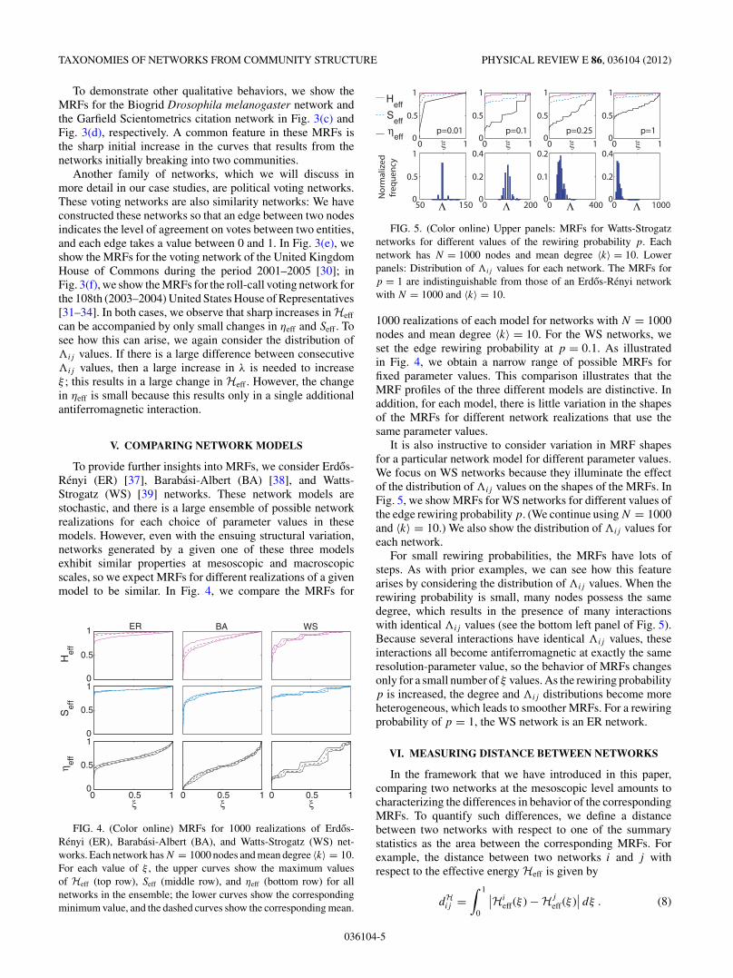
To demonstrate other qualitative behaviors, we show theMRFs for the Biogrid Drosophila melanogaster network andthe Garfield Scientometrics citation network in Fig. 3(c) andFig. 3(d), respectively. A common feature in these MRFs isthe sharp initial increase in the curves that results from thenetworks initially breaking into two communities.
Another family of networks, which we will discuss inmore detail in our case studies, are political voting networks.These voting networks are also similarity networks: We haveconstructed these networks so that an edge between two nodesindicates the level of agreement on votes between two entities,and each edge takes a value between 0 and 1. In Fig. 3(e), weshow the MRFs for the voting network of the United KingdomHouse of Commons during the period 2001–2005 [30]; inFig. 3(f), we show the MRFs for the roll-call voting network forthe 108th (2003–2004) United States House of Representatives[31–34]. In both cases, we observe that sharp increases in Heffcan be accompanied by only small changes in $eff and Seff . Tosee how this can arise, we again consider the distribution of#ij values. If there is a large difference between consecutive#ij values, then a large increase in ! is needed to increase& ; this results in a large change in Heff . However, the changein $eff is small because this results only in a single additionalantiferromagnetic interaction.
V. COMPARING NETWORK MODELS
To provide further insights into MRFs, we consider Erdos-Renyi (ER) [37], Barabasi-Albert (BA) [38], and Watts-Strogatz (WS) [39] networks. These network models arestochastic, and there is a large ensemble of possible networkrealizations for each choice of parameter values in thesemodels. However, even with the ensuing structural variation,networks generated by a given one of these three modelsexhibit similar properties at mesoscopic and macroscopicscales, so we expect MRFs for different realizations of a givenmodel to be similar. In Fig. 4, we compare the MRFs for
0
0.5
1
Hef
f
ER
0
0.5
1
Sef
f
0 0.5 10
0.5
1
" eff
BA
0 0.5 1!
WS
0 0.5 1! !
FIG. 4. (Color online) MRFs for 1000 realizations of Erdos-Renyi (ER), Barabasi-Albert (BA), and Watts-Strogatz (WS) net-works. Each network has N = 1000 nodes and mean degree $k% = 10.For each value of & , the upper curves show the maximum valuesof Heff (top row), Seff (middle row), and $eff (bottom row) for allnetworks in the ensemble; the lower curves show the correspondingminimum value, and the dashed curves show the corresponding mean.
!
!
Nor
mal
ized
freq
uenc
y
p=0.01 p=0.1 p=0.25 p=1
1
0
0.5
1
0
0.5
1
0
0.5
1
0
0.5
1
0
0.5
0.4
0
0.2
0.4
0
0.2
0.2
0
0.1
0 1 0 1 0 1 0 1
50 150 0 200 0 400 0 1000
Heff
Seff
"eff
FIG. 5. (Color online) Upper panels: MRFs for Watts-Strogatznetworks for different values of the rewiring probability p. Eachnetwork has N = 1000 nodes and mean degree $k% = 10. Lowerpanels: Distribution of #ij values for each network. The MRFs forp = 1 are indistinguishable from those of an Erdos-Renyi networkwith N = 1000 and $k% = 10.
1000 realizations of each model for networks with N = 1000nodes and mean degree $k% = 10. For the WS networks, weset the edge rewiring probability at p = 0.1. As illustratedin Fig. 4, we obtain a narrow range of possible MRFs forfixed parameter values. This comparison illustrates that theMRF profiles of the three different models are distinctive. Inaddition, for each model, there is little variation in the shapesof the MRFs for different network realizations that use thesame parameter values.
It is also instructive to consider variation in MRF shapesfor a particular network model for different parameter values.We focus on WS networks because they illuminate the effectof the distribution of#ij values on the shapes of the MRFs. InFig. 5, we show MRFs for WS networks for different values ofthe edge rewiring probability p. (We continue using N = 1000and $k% = 10.) We also show the distribution of#ij values foreach network.
For small rewiring probabilities, the MRFs have lots ofsteps. As with prior examples, we can see how this featurearises by considering the distribution of #ij values. When therewiring probability is small, many nodes possess the samedegree, which results in the presence of many interactionswith identical #ij values (see the bottom left panel of Fig. 5).Because several interactions have identical #ij values, theseinteractions all become antiferromagnetic at exactly the sameresolution-parameter value, so the behavior of MRFs changesonly for a small number of & values. As the rewiring probabilityp is increased, the degree and #ij distributions become moreheterogeneous, which leads to smoother MRFs. For a rewiringprobability of p = 1, the WS network is an ER network.
VI. MEASURING DISTANCE BETWEEN NETWORKS
In the framework that we have introduced in this paper,comparing two networks at the mesoscopic level amounts tocharacterizing the differences in behavior of the correspondingMRFs. To quantify such differences, we define a distancebetween two networks with respect to one of the summarystatistics as the area between the corresponding MRFs. Forexample, the distance between two networks i and j withrespect to the effective energy Heff is given by
dHij =
# 1
0
$$Hieff(& ) ! Hj
eff(& )$$ d& . (8)
036104-5

JUKKA-PEKKA ONNELA et al. PHYSICAL REVIEW E 86, 036104 (2012)
TABLE I. Network categories, the total number of networksassigned to each category, and the number of networks from eachcategory included in the taxonomy in Fig. 6. For the full taxonomythat uses all 746 networks, see Fig. 1 of the Supplemental Material.
Category All networks Taxonomy networks
Political: voting 285 23Facebook 100 15Fungal 65 12Synthetic 58 0Financial 54 6Metabolic 43 15Social 26 26Political: cosponsorship 26 26Other 23 0Protein interaction 22 22Political: committee 16 16Brain 12 12Language 8 8Collaboration 8 8Total 746 189
For the effective entropy and effective number of communities,the distances are given by dS
ij =% 1
0 |Sieff(& ) ! S
jeff(& )| d& and
d$ij =
% 10 |$i
eff(& ) ! $jeff(& )| d& , respectively.
We represent the resulting three sets of distances (computedfor each pair of networks from the 746 networks that weconsider; see Table I) in matrix form as DH, DS , and D$. Thesedistance measures have several desirable properties. First, theycompare MRFs across all network scales (i.e., for all values of& ); second, each distance is bounded between 0 and 1; third,the distances are easy to interpret, as each of them correspondsto the geometric area between (a certain dimension of) a pairof MRFs; and finally, we find a posteriori that these distancescan be used to cluster networks accurately (see the discussionsbelow).
We have computed MRFs for the energy H, entropy S,and number of communities $, but we can proceed similarlywith any desired summary statistic. If two diagnostics providesimilar information, then one of them can be excluded withoutsignificant loss of information. We checked whether thesummary statistics were sufficiently different—for the setof networks that we considered—for it to be worthwhile toinclude all of them by calculating the Pearson correlationcoefficient between their corresponding distance measures.The correlations between the pairs of distances are r(dH
ij ,dSij ) .=
0.36, r(dHij ,d
$ij ) .= 0.24, and r(dS
ij ,d$ij ) .= 0.58. These correla-
tions are not sufficiently high to justify excluding any of thesummary statistics.
In the interest of parsimony—and given the nonvanishingcorrelations between the distance measures—we reduce thenumber of distance measures using principal componentanalysis (PCA) [40]. Starting with N networks, we createa 1
2N (N ! 1) & 3 matrix in which each column correspondsto the vector representation of the upper triangle of one ofthe distance matrices DH, DS , D$, and we perform a PCAon this matrix. We then define a distance matrix Dp withelements d
pij = wHdH
ij + wSdSij + w$d
$ij , where the weights
are the coefficients for the first principal component, and
we normalize the sum of squared coefficients to unity. Thecoefficients are wH
.= 0.24, wS.= 0.79, and w$
.= 0.57. Thefirst component accounts for about 69% of the variance, sothe distance matrix Dp provides a reasonable single-variableprojection of the distance matrices DH, DS , and D$.
It is important that the distance measures for comparingnetworks are robust to small perturbations in network structure.Because many of the networks that we study are constructedempirically, they might contain false positives and falsenegatives. In other words, the networks might falsely identifya relationship where none exists, and they also might fail toidentify an existing relationship. Consequently, the topologyand edge weights of an observed network might be slightlydifferent than those of the actual underlying network. To testthe robustness of our distance measures to such observationalerrors, we recalculate the MRFs for a subset of relatively smallunweighted networks in which, for each network, we rewirea number of edges corresponding to a given percentage ofthe total number of edges (5%, 10%, 20%, 50%, or 100%).See Appendix A for more details. (We study networks withup to 1000 nodes and consider only a subset of 25 networksbecause of the computational costs of rewiring a large numberof networks multiple times; however, we have performed thesame investigation for five different subsets of 25 networks andobtained similar results. We list the networks in each subsetin Table I of the Supplemental Material.) We investigate tworewiring mechanisms: one in which the degree distribution ismaintained, where we also ensure after each rewiring that thenetwork consists of a single connected component; and anotherin which the only constraint is that the network continuesto consist of a single connected component after each edgerewiring [41]. We find in both cases that the structures ofthe block-diagonalized distance matrices for the 25 networks(see Figs. 14 and 15 in Appendix A) are robust to randomperturbations of the networks, thereby suggesting that ourMRF distance measures are not sensitive to small structuralperturbations.
VII. CLUSTERING NETWORKS
We assign each of the 746 networks to a category basedon its type (see Table I). Due to the varying availability ofdifferent types of network data, the networks that we considerare not distributed evenly across these categories. Many of thenetworks are either different temporal snapshots of the samesystem or different realizations of the same type of network.To have a more balanced distribution across the differentcategories, we focus on 189 of the 746 networks. We includeonly categories for which we have eight or more networks, andwe select a subset of networks (uniformly at random) fromeach of the larger categories. We also exclude all syntheticnetworks. See Sec. IV of the Supplemental Material for thelist of networks that we consider and Fig. 1 in Sec. II of theSupplemental Material for a dendrogram showing a taxonomythat we constructed using all 746 networks.
Our primary reason for assigning each network to a categoryis to use such an external categorization to help assess thequality of taxonomies produced by the unsupervised MRFclustering. For each way of computing distance, we constructa dendrogram for the set of networks using average linkage
036104-6
TAXONOMIES OF NETWORKS FROM COMMUNITY STRUCTURE PHYSICAL REVIEW E 86, 036104 (2012)
0
0.1
0.2
0.3
0.4
SocialFacebook
Political: cosponsorshipPolitical: voting
Political: committeeProtein interactionMetabolicBrainFungalFinancialLanguageCollaboration
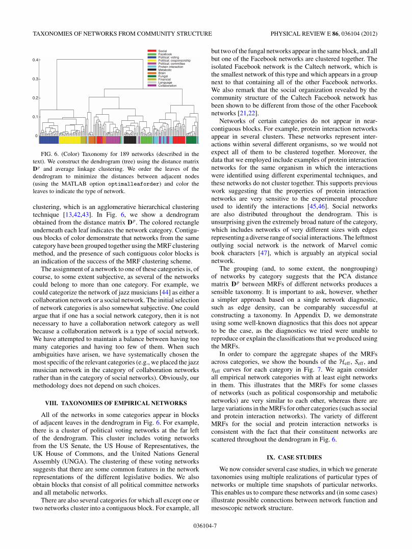
FIG. 6. (Color) Taxonomy for 189 networks (described in thetext). We construct the dendrogram (tree) using the distance matrixDp and average linkage clustering. We order the leaves of thedendrogram to minimize the distances between adjacent nodes(using the MATLAB option optimalleaforder) and color theleaves to indicate the type of network.
clustering, which is an agglomerative hierarchical clusteringtechnique [13,42,43]. In Fig. 6, we show a dendrogramobtained from the distance matrix Dp. The colored rectangleunderneath each leaf indicates the network category. Contigu-ous blocks of color demonstrate that networks from the samecategory have been grouped together using the MRF clusteringmethod, and the presence of such contiguous color blocks isan indication of the success of the MRF clustering scheme.
The assignment of a network to one of these categories is, ofcourse, to some extent subjective, as several of the networkscould belong to more than one category. For example, wecould categorize the network of jazz musicians [44] as either acollaboration network or a social network. The initial selectionof network categories is also somewhat subjective. One couldargue that if one has a social network category, then it is notnecessary to have a collaboration network category as wellbecause a collaboration network is a type of social network.We have attempted to maintain a balance between having toomany categories and having too few of them. When suchambiguities have arisen, we have systematically chosen themost specific of the relevant categories (e.g., we placed the jazzmusician network in the category of collaboration networksrather than in the category of social networks). Obviously, ourmethodology does not depend on such choices.
VIII. TAXONOMIES OF EMPIRICAL NETWORKS
All of the networks in some categories appear in blocksof adjacent leaves in the dendrogram in Fig. 6. For example,there is a cluster of political voting networks at the far leftof the dendrogram. This cluster includes voting networksfrom the US Senate, the US House of Representatives, theUK House of Commons, and the United Nations GeneralAssembly (UNGA). The clustering of these voting networkssuggests that there are some common features in the networkrepresentations of the different legislative bodies. We alsoobtain blocks that consist of all political committee networksand all metabolic networks.
There are also several categories for which all except one ortwo networks cluster into a contiguous block. For example, all
but two of the fungal networks appear in the same block, and allbut one of the Facebook networks are clustered together. Theisolated Facebook network is the Caltech network, which isthe smallest network of this type and which appears in a groupnext to that containing all of the other Facebook networks.We also remark that the social organization revealed by thecommunity structure of the Caltech Facebook network hasbeen shown to be different from those of the other Facebooknetworks [21,22].
Networks of certain categories do not appear in near-contiguous blocks. For example, protein interaction networksappear in several clusters. These networks represent inter-actions within several different organisms, so we would notexpect all of them to be clustered together. Moreover, thedata that we employed include examples of protein interactionnetworks for the same organism in which the interactionswere identified using different experimental techniques, andthese networks do not cluster together. This supports previouswork suggesting that the properties of protein interactionnetworks are very sensitive to the experimental procedureused to identify the interactions [45,46]. Social networksare also distributed throughout the dendrogram. This isunsurprising given the extremely broad nature of the category,which includes networks of very different sizes with edgesrepresenting a diverse range of social interactions. The leftmostoutlying social network is the network of Marvel comicbook characters [47], which is arguably an atypical socialnetwork.
The grouping (and, to some extent, the nongrouping)of networks by category suggests that the PCA distancematrix Dp between MRFs of different networks produces asensible taxonomy. It is important to ask, however, whethera simpler approach based on a single network diagnostic,such as edge density, can be comparably successful atconstructing a taxonomy. In Appendix D, we demonstrateusing some well-known diagnostics that this does not appearto be the case, as the diagnostics we tried were unable toreproduce or explain the classifications that we produced usingthe MRFs.
In order to compare the aggregate shapes of the MRFsacross categories, we show the bounds of the Heff , Seff , and$eff curves for each category in Fig. 7. We again considerall empirical network categories with at least eight networksin them. This illustrates that the MRFs for some classesof networks (such as political cosponsorship and metabolicnetworks) are very similar to each other, whereas there arelarge variations in the MRFs for other categories (such as socialand protein interaction networks). The variety of differentMRFs for the social and protein interaction networks isconsistent with the fact that their constituent networks arescattered throughout the dendrogram in Fig. 6.
IX. CASE STUDIES
We now consider several case studies, in which we generatetaxonomies using multiple realizations of particular types ofnetworks or multiple time snapshots of particular networks.This enables us to compare these networks and (in some cases)illustrate possible connections between network function andmesoscopic network structure.
036104-7
JUKKA-PEKKA ONNELA et al. PHYSICAL REVIEW E 86, 036104 (2012)
Social Facebook Political: voting
Political: cosponsorship Political: committee Protein interaction
Metabolic Brain Fungal
Financial
!
Language Collaboration
!effeffeff
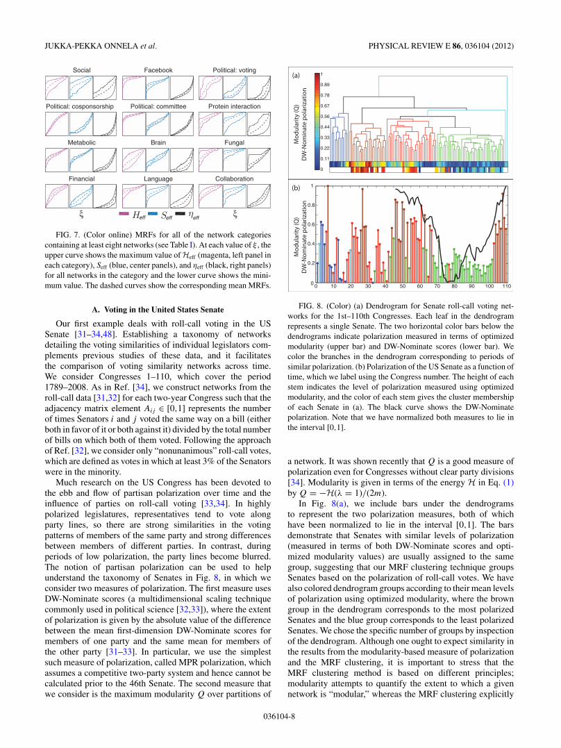
FIG. 7. (Color online) MRFs for all of the network categoriescontaining at least eight networks (see Table I). At each value of & , theupper curve shows the maximum value of Heff (magenta, left panel ineach category), Seff (blue, center panels), and $eff (black, right panels)for all networks in the category and the lower curve shows the mini-mum value. The dashed curves show the corresponding mean MRFs.
A. Voting in the United States Senate
Our first example deals with roll-call voting in the USSenate [31–34,48]. Establishing a taxonomy of networksdetailing the voting similarities of individual legislators com-plements previous studies of these data, and it facilitatesthe comparison of voting similarity networks across time.We consider Congresses 1–110, which cover the period1789–2008. As in Ref. [34], we construct networks from theroll-call data [31,32] for each two-year Congress such that theadjacency matrix element Aij # [0,1] represents the numberof times Senators i and j voted the same way on a bill (eitherboth in favor of it or both against it) divided by the total numberof bills on which both of them voted. Following the approachof Ref. [32], we consider only “nonunanimous” roll-call votes,which are defined as votes in which at least 3% of the Senatorswere in the minority.
Much research on the US Congress has been devoted tothe ebb and flow of partisan polarization over time and theinfluence of parties on roll-call voting [33,34]. In highlypolarized legislatures, representatives tend to vote alongparty lines, so there are strong similarities in the votingpatterns of members of the same party and strong differencesbetween members of different parties. In contrast, duringperiods of low polarization, the party lines become blurred.The notion of partisan polarization can be used to helpunderstand the taxonomy of Senates in Fig. 8, in which weconsider two measures of polarization. The first measure usesDW-Nominate scores (a multidimensional scaling techniquecommonly used in political science [32,33]), where the extentof polarization is given by the absolute value of the differencebetween the mean first-dimension DW-Nominate scores formembers of one party and the same mean for members ofthe other party [31–33]. In particular, we use the simplestsuch measure of polarization, called MPR polarization, whichassumes a competitive two-party system and hence cannot becalculated prior to the 46th Senate. The second measure thatwe consider is the maximum modularity Q over partitions of
0
0.11
0.22
0.33
0.44
0.56
0.67
0.78
0.89
1
10 20 30 40 50 60 70 80 90 100 1100
0.2
0.4
0.6
0.8
1
0
Mod
ular
ity (Q
)D
W-N
omin
ate
pola
rizat
ion
Mod
ular
ity (Q
)D
W-N
omin
ate
pola
rizat
ion
(a)
(b)
FIG. 8. (Color) (a) Dendrogram for Senate roll-call voting net-works for the 1st–110th Congresses. Each leaf in the dendrogramrepresents a single Senate. The two horizontal color bars below thedendrograms indicate polarization measured in terms of optimizedmodularity (upper bar) and DW-Nominate scores (lower bar). Wecolor the branches in the dendrogram corresponding to periods ofsimilar polarization. (b) Polarization of the US Senate as a function oftime, which we label using the Congress number. The height of eachstem indicates the level of polarization measured using optimizedmodularity, and the color of each stem gives the cluster membershipof each Senate in (a). The black curve shows the DW-Nominatepolarization. Note that we have normalized both measures to lie inthe interval [0,1].
a network. It was shown recently that Q is a good measure ofpolarization even for Congresses without clear party divisions[34]. Modularity is given in terms of the energy H in Eq. (1)by Q = !H(! = 1)/(2m).
In Fig. 8(a), we include bars under the dendrogramsto represent the two polarization measures, both of whichhave been normalized to lie in the interval [0,1]. The barsdemonstrate that Senates with similar levels of polarization(measured in terms of both DW-Nominate scores and opti-mized modularity values) are usually assigned to the samegroup, suggesting that our MRF clustering technique groupsSenates based on the polarization of roll-call votes. We havealso colored dendrogram groups according to their mean levelsof polarization using optimized modularity, where the browngroup in the dendrogram corresponds to the most polarizedSenates and the blue group corresponds to the least polarizedSenates. We chose the specific number of groups by inspectionof the dendrogram. Although one ought to expect similarity inthe results from the modularity-based measure of polarizationand the MRF clustering, it is important to stress that theMRF clustering method is based on different principles;modularity attempts to quantify the extent to which a givennetwork is “modular,” whereas the MRF clustering explicitly
036104-8

TAXONOMIES OF NETWORKS FROM COMMUNITY STRUCTURE PHYSICAL REVIEW E 86, 036104 (2012)
0 0.2 0.4 0.6 0.8 10
0.2
0.4
0.6
0.8
1
!
Hef
f
0 1 2 30
0.2
0.4
0.6
0.8
1
#ij
P(#
ij$x)
Senate 85Senate 108
Senate 85Senate 108
(a) (b)
FIG. 9. (Color online) Comparison of the (low-polarization) 85thSenate and the (high-polarization) 108th Senate. The panels show (a)the Heff MRFs and (b) the cumulative distributions of #ij values.
compares the differences in modular structures between anytwo networks at all scales.
In Fig. 8(a), we also show the clusters that we obtainedfor the Senate. They closely match the different periodsof polarization that have been identified using optimizedmodularity and DW-Nominate [34]. The cluster with thehighest mean polarization (shown in brown) consists ofSenates 7, 26–29, 44, 46–51, 53, 55, 66, and 104–110. The104th–110th Congresses correspond to a period of extremelyhigh polarization following the 1994 “Republican Revolution,”in which the Republican party earned majority status in theHouse of Representatives for the first time in more than 40years [31,33,34]. The cluster with the second highest meanpolarization (shown in red) includes several contiguous blocksof Senates, such as those from Congresses 21–25, 35–39, and56–61. The 21st–25th Congresses (1829–1839) correspondedto a period of partisan conflict between supporters of JohnQuincy Adams and Andrew Jackson; it lasted until theemergence of the Whigs and the Democratic Party in the 25thCongress [34,49]. The American Civil War started during the37th Congress, and a third party known as the Populist Partywas strong during the 56th–58th Congresses.
The main differences between different clusters occur inthe Heff response functions. For the most polarized Senates,there is a sharp shoulder in the Heff MRF that becomesless pronounced as the polarization decreases. We illustratethis in Fig. 9, in which we compare the Heff MRFs for the(low-polarization) 85th and (high-polarization) 108th Senates.The shoulder in the Heff curve for the 108th Senate isvery pronounced, which can be explained by considering thedistribution of#ij values. The 108th Senate has a bimodal#ij
distribution that contains a trough at#ij = 1. Recall that#ij =Aij/Pij , so #ij compares the observed voting similarity Aij
of legislators i and j with the similarity Pij = kikj /(2m) ex-pected from random voting. If#ij < 1, legislators i and j votedifferently more frequently than expected (with respect to thechosen null model); if #ij > 1, they vote more similarly thanexpected. Therefore, the peaks in the #ij distribution aboveand below 1 correspond, respectively, to intraparty and inter-party voting blocs. In a Senate with low polarization, legisla-tors from different parties often vote in the same manner, so thevalues of#ij no longer separate two distinct types of behavior.
We also examined roll-call voting networks in the US Houseof Representatives and found many similar features as the ones
that we have presented for the US Senate. For example, thehighly polarized 104th–110th Congresses, which followed the“Republican Revolution,” appear in the same cluster for boththe House and Senate. We also observed some differences inthe clusters for the two chambers. For example, the 78th–102ndSenates all appear in the same cluster. For the House, however,Congresses 80, 88, 89, and 98–102 are not in the same clusteras the other Congresses between 78 and 102; instead, theyare assigned to a cluster that also includes the 26th–28thHouses. This was a particularly eventful period: The 25thCongress saw the emergence of the Whigs and the DemocraticParty, and the abolitionist movement was also prevalent(e.g., the Amistad seizure occurred in 1839 during the 26thCongress).
B. Voting in the United Nations General Assembly
The United Nations General Assembly (UNGA) is one ofthe principal organs of the United Nations (UN), and it is theonly part of the UN in which all member nations have equalrepresentation. Although most resolutions are neither legallynor practically enforceable because the General Assemblylacks enforcement powers on most issues, it is the only forumin which a large number of states meet and vote regularly oninternational issues. It also provides an interesting point ofcomparison with roll-call voting in the US Congress, as thelevel of agreement on UN resolutions tends to be much higherthan that in the Senate and House [50].
We study voting for the 1st–63rd sessions (covering theperiod 1946–2008), where each session corresponds to a year[51]. For each session, we define an adjacency matrix A whoseelements Aij represent the number of times countries i andj voted in the same manner in a session (i.e., the sum ofthe number of times both countries voted yea on the sameresolution, both countries voted nay on the same resolution, orboth countries abstained from voting on the same resolution)divided by the total number of resolutions on which the UNGAvoted in a session. The matrix A, with elements Aij # [0,1],thereby represents a (similarity) network of weighted edgesbetween countries.
We cluster UNGA sessions by comparing MRFs forthe corresponding voting networks. In Fig. 10, we plot a
1977
1954
19
49
1956
19
58
1995
19
5119
57
1963
1970
1960
1969
19
68
1952
1947
1953
1967
19
59
1961
1966
19
7119
62
1965
19
55
1996
19
94
1997
19
98
2000
2002
1999
2001
20
08
2007
20
06
1992
19
93
2005
20
04
2003
19
75
1973
19
74
1972
19
46
1950
19
48
1978
19
76
1980
19
79
1982
19
81
1986
19
83
1985
19
87
1984
19
89
1988
19
90
1991
1979!1991 (excl. 1980)1992!2008 (excl. 1995)1946, 1948, 1950
FIG. 10. (Color online) Dendrogram for the United Nations Gen-eral Assembly resolution voting network for the 1st–63rd sessions(excluding the 19th session), covering the period 1946–2008. Eachleaf in the dendrogram represents a single session. In the main text,we discuss the coloring of groups of dendrogram branches.
036104-9
JUKKA-PEKKA ONNELA et al. PHYSICAL REVIEW E 86, 036104 (2012)
dendrogram of the UNGA sessions and highlight some ofthe clusters, which correspond to notable periods in the recenthistory of international relations. The red cluster in the middleof the dendrogram consists of all post-Cold War sessions(1992–2008) except 1995. This group forms a larger clusterwith some UNGA sessions from the 1970s and a clusterconsisting of 1946, 1948, and 1950. These last three sessions(which are shown in magenta) are all noteworthy: 1946 wasthe first session of the UNGA, the Universal Declaration ofHuman Rights was introduced during the 1948 session, andthe “Uniting for Peace” resolution was passed during the 1950session. At the rightmost part of the dendrogram, we color inblack a group that consists of all sessions from 1979 to 1991(excluding 1980). The beginning of this period marked theend of detente between the Soviet Union and the United Statesfollowing the former’s invasion of Afghanistan at the end of1979, and the end of this period saw the end of the Cold War.The large blue cluster in the leftmost part of the dendrogramconsists primarily of sessions from before 1971 (though it alsoincludes the sessions in 1977 and 1995).
C. Facebook
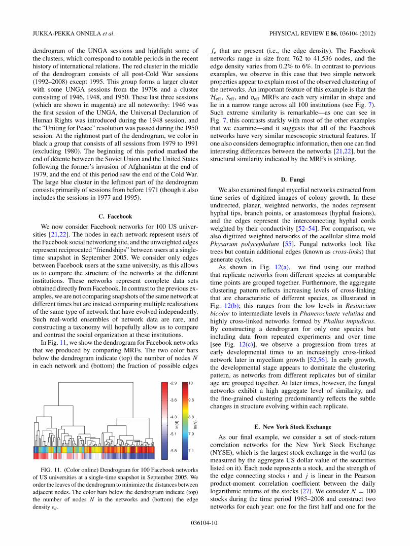
We now consider Facebook networks for 100 US univer-sities [21,22]. The nodes in each network represent users ofthe Facebook social networking site, and the unweighted edgesrepresent reciprocated “friendships” between users at a single-time snapshot in September 2005. We consider only edgesbetween Facebook users at the same university, as this allowsus to compare the structure of the networks at the differentinstitutions. These networks represent complete data setsobtained directly from Facebook. In contrast to the previous ex-amples, we are not comparing snapshots of the same network atdifferent times but are instead comparing multiple realizationsof the same type of network that have evolved independently.Such real-world ensembles of network data are rare, andconstructing a taxonomy will hopefully allow us to compareand contrast the social organization at these institutions.
In Fig. 11, we show the dendrogram for Facebook networksthat we produced by comparing MRFs. The two color barsbelow the dendrogram indicate (top) the number of nodes Nin each network and (bottom) the fraction of possible edges
ln(N
)
7.1
7.9
8.8
9.6
10
ln(d
)
-5.8
-5.1
-4.3
-3.6
-2.9
FIG. 11. (Color online) Dendrogram for 100 Facebook networksof US universities at a single-time snapshot in September 2005. Weorder the leaves of the dendrogram to minimize the distances betweenadjacent nodes. The color bars below the dendrogram indicate (top)the number of nodes N in the networks and (bottom) the edgedensity ed .
fe that are present (i.e., the edge density). The Facebooknetworks range in size from 762 to 41,536 nodes, and theedge density varies from 0.2% to 6%. In contrast to previousexamples, we observe in this case that two simple networkproperties appear to explain most of the observed clustering ofthe networks. An important feature of this example is that theHeff , Seff , and $eff MRFs are each very similar in shape andlie in a narrow range across all 100 institutions (see Fig. 7).Such extreme similarity is remarkable—as one can see inFig. 7, this contrasts starkly with most of the other examplesthat we examine—and it suggests that all of the Facebooknetworks have very similar mesoscopic structural features. Ifone also considers demographic information, then one can findinteresting differences between the networks [21,22], but thestructural similarity indicated by the MRFs is striking.
D. Fungi
We also examined fungal mycelial networks extracted fromtime series of digitized images of colony growth. In theseundirected, planar, weighted networks, the nodes representhyphal tips, branch points, or anastomoses (hyphal fusions),and the edges represent the interconnecting hyphal cordsweighted by their conductivity [52–54]. For comparison, wealso digitized weighted networks of the acellular slime moldPhysarum polycephalum [55]. Fungal networks look liketrees but contain additional edges (known as cross-links) thatgenerate cycles.
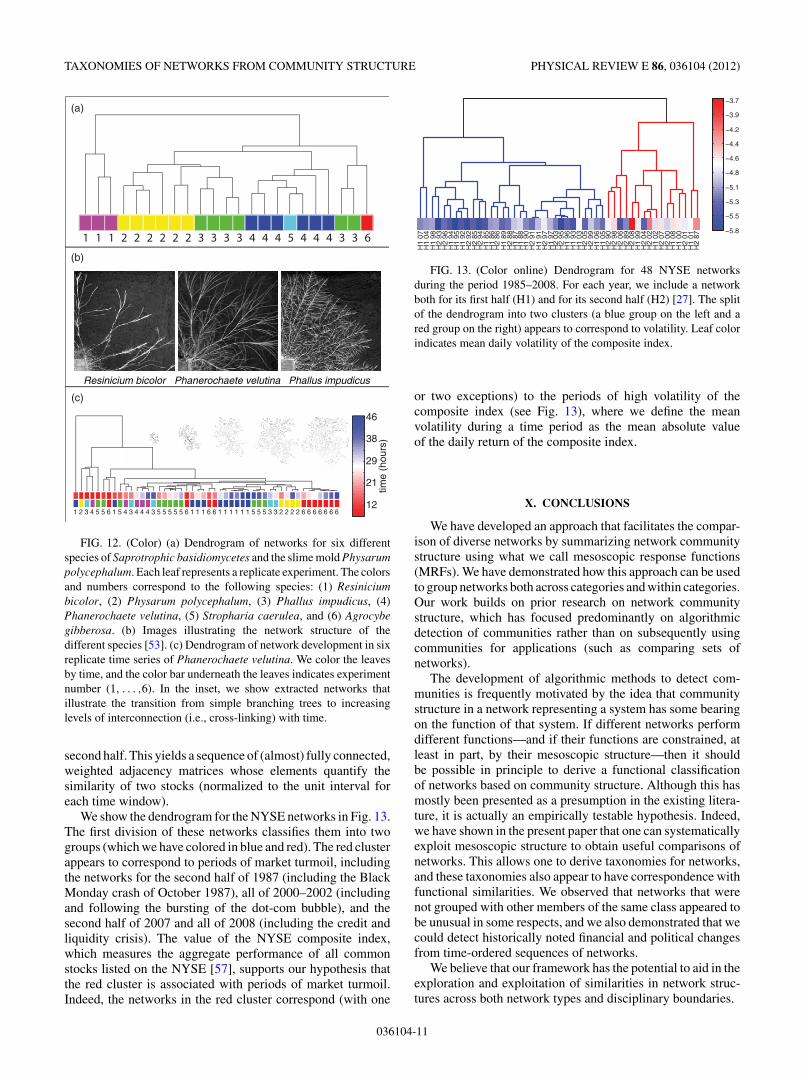
As shown in Fig. 12(a), we find using our methodthat replicate networks from different species at comparabletime points are grouped together. Furthermore, the aggregateclustering pattern reflects increasing levels of cross-linkingthat are characteristic of different species, as illustrated inFig. 12(b); this ranges from the low levels in Resiniciumbicolor to intermediate levels in Phanerochaete velutina andhighly cross-linked networks formed by Phallus impudicus.By constructing a dendrogram for only one species butincluding data from repeated experiments and over time[see Fig. 12(c)], we observe a progression from trees atearly developmental times to an increasingly cross-linkednetwork later in mycelium growth [52,56]. In early growth,the developmental stage appears to dominate the clusteringpattern, as networks from different replicates but of similarage are grouped together. At later times, however, the fungalnetworks exhibit a high aggregate level of similarity, andthe fine-grained clustering predominantly reflects the subtlechanges in structure evolving within each replicate.
E. New York Stock Exchange
As our final example, we consider a set of stock-returncorrelation networks for the New York Stock Exchange(NYSE), which is the largest stock exchange in the world (asmeasured by the aggregate US dollar value of the securitieslisted on it). Each node represents a stock, and the strength ofthe edge connecting stocks i and j is linear in the Pearsonproduct-moment correlation coefficient between the dailylogarithmic returns of the stocks [27]. We consider N = 100stocks during the time period 1985–2008 and construct twonetworks for each year: one for the first half and one for the
036104-10
TAXONOMIES OF NETWORKS FROM COMMUNITY STRUCTURE PHYSICAL REVIEW E 86, 036104 (2012)
time
(hou
rs)
12
21
29
38
46
2 2 2 3 3 3 3 4 4 4 5 41 1 1 2 2 2 4 4 3 3 6
1 2 3 4 5 5 6 1 5 4 3 4 4 4 3 5 5 5 5 5 6 1 1 1 6 6 1 1 1 1 1 1 5 5 5 3 3 2 2 2 2 6 6 6 6 6 6 6
Resinicium bicolor Phanerochaete velutina Phallus impudicus
(a)
(b)
(c)
FIG. 12. (Color) (a) Dendrogram of networks for six differentspecies of Saprotrophic basidiomycetes and the slime mold Physarumpolycephalum. Each leaf represents a replicate experiment. The colorsand numbers correspond to the following species: (1) Resiniciumbicolor, (2) Physarum polycephalum, (3) Phallus impudicus, (4)Phanerochaete velutina, (5) Stropharia caerulea, and (6) Agrocybegibberosa. (b) Images illustrating the network structure of thedifferent species [53]. (c) Dendrogram of network development in sixreplicate time series of Phanerochaete velutina. We color the leavesby time, and the color bar underneath the leaves indicates experimentnumber (1, . . . ,6). In the inset, we show extracted networks thatillustrate the transition from simple branching trees to increasinglevels of interconnection (i.e., cross-linking) with time.
second half. This yields a sequence of (almost) fully connected,weighted adjacency matrices whose elements quantify thesimilarity of two stocks (normalized to the unit interval foreach time window).
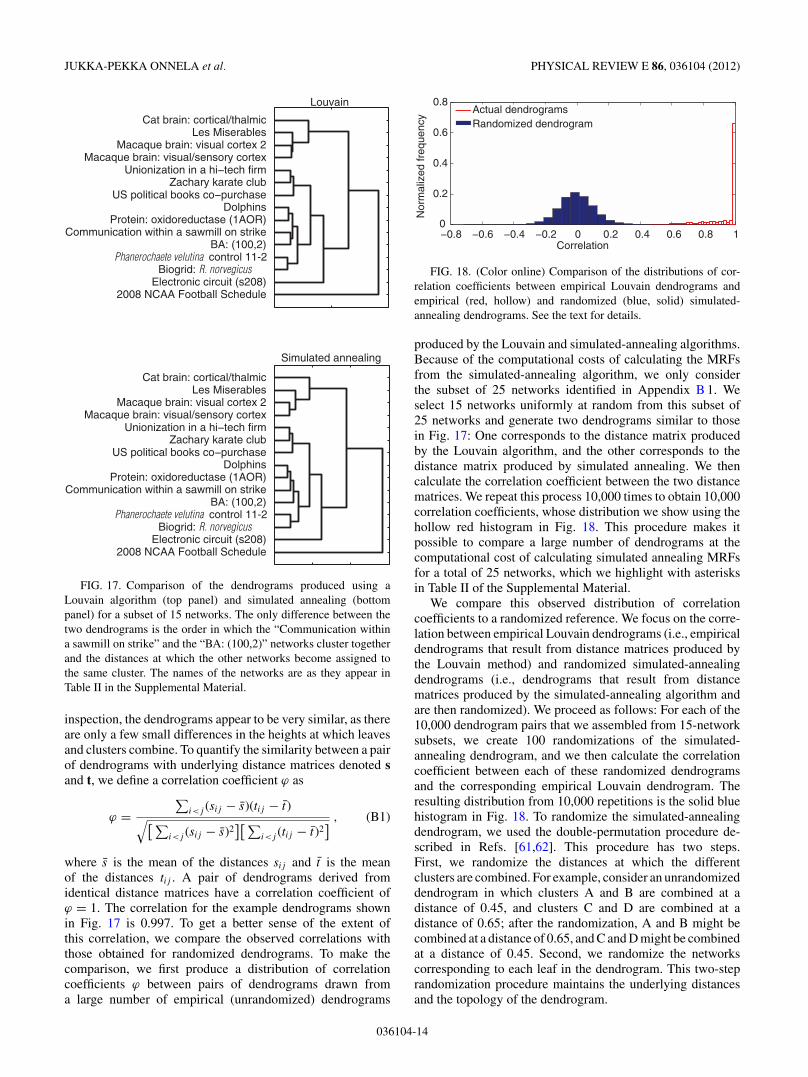
We show the dendrogram for the NYSE networks in Fig. 13.The first division of these networks classifies them into twogroups (which we have colored in blue and red). The red clusterappears to correspond to periods of market turmoil, includingthe networks for the second half of 1987 (including the BlackMonday crash of October 1987), all of 2000–2002 (includingand following the bursting of the dot-com bubble), and thesecond half of 2007 and all of 2008 (including the credit andliquidity crisis). The value of the NYSE composite index,which measures the aggregate performance of all commonstocks listed on the NYSE [57], supports our hypothesis thatthe red cluster is associated with periods of market turmoil.Indeed, the networks in the red cluster correspond (with one
H1
07H
1 04
H1
98H
2 93
H2
96H
1 94
H1
95H
1 92
H2
92H
2 85
H2
94H
1 85
H1
86H
2 86
H1
89H
2 88
H1
87H
1 88
H1
90H
2 91
H1
91H
2 97
H1
97H
2 03
H2
95H
1 96
H1
93H
1 03
H2
05H
2 99
H1
06H
1 05
H2
90H
2 98
H2
06H
2 89
H2
08H
1 99
H2
04H
2 02
H1
02H
2 07
H2
00H
1 08
H1
00H
2 01
H1
01H
2 87
!5.8
!5.5
!5.3
!5.1
!4.8
!4.6
!4.4
!4.2
!3.9
!3.7
FIG. 13. (Color online) Dendrogram for 48 NYSE networksduring the period 1985–2008. For each year, we include a networkboth for its first half (H1) and for its second half (H2) [27]. The splitof the dendrogram into two clusters (a blue group on the left and ared group on the right) appears to correspond to volatility. Leaf colorindicates mean daily volatility of the composite index.
or two exceptions) to the periods of high volatility of thecomposite index (see Fig. 13), where we define the meanvolatility during a time period as the mean absolute valueof the daily return of the composite index.
X. CONCLUSIONS
We have developed an approach that facilitates the compar-ison of diverse networks by summarizing network communitystructure using what we call mesoscopic response functions(MRFs). We have demonstrated how this approach can be usedto group networks both across categories and within categories.Our work builds on prior research on network communitystructure, which has focused predominantly on algorithmicdetection of communities rather than on subsequently usingcommunities for applications (such as comparing sets ofnetworks).
The development of algorithmic methods to detect com-munities is frequently motivated by the idea that communitystructure in a network representing a system has some bearingon the function of that system. If different networks performdifferent functions—and if their functions are constrained, atleast in part, by their mesoscopic structure—then it shouldbe possible in principle to derive a functional classificationof networks based on community structure. Although this hasmostly been presented as a presumption in the existing litera-ture, it is actually an empirically testable hypothesis. Indeed,we have shown in the present paper that one can systematicallyexploit mesoscopic structure to obtain useful comparisons ofnetworks. This allows one to derive taxonomies for networks,and these taxonomies also appear to have correspondence withfunctional similarities. We observed that networks that werenot grouped with other members of the same class appeared tobe unusual in some respects, and we also demonstrated that wecould detect historically noted financial and political changesfrom time-ordered sequences of networks.
We believe that our framework has the potential to aid in theexploration and exploitation of similarities in network struc-tures across both network types and disciplinary boundaries.
036104-11

JUKKA-PEKKA ONNELA et al. PHYSICAL REVIEW E 86, 036104 (2012)
ACKNOWLEDGMENTS
We are particularly grateful to A. D’Angelo and Facebook,A. Merdzanovic, M. E. J. Newman, E. Voeten, and Voteview[31] (maintained by K. Poole and H. Rosenthal) for data.We thank A. Lewis, G. Villar, S. Agarwal, D. Smith, andthe anonymous referees for useful suggestions. We adaptedcode originally written by R. Guimera for the simulated-annealing algorithm and code by R. Lambiotte for the Louvainalgorithm. This research was supported in part by the FulbrightProgram (J.P.O.) and NIH grant P01 AG-031093 (J.P.O.), theJames S. McDonnell Foundation (M.A.P.: 220020177), NSF(P.J.M.: DMS-0645369), and EPSRC and BBSRC (N.S.J.:EP/I005765/1, EP/I005986/1, and BBD0201901).
APPENDIX A: ROBUSTNESS OF CLUSTERING
To examine the robustness of our clustering to falsepositives (false links) and false negatives (false nonlinks), weconsider two network rewiring mechanisms, and we applythe rewiring to each network among 25 of the 746 networksin Table II in the Supplemental Material. We highlight these25 networks in that table. (In the Supplemental Material, wealso consider five additional subsets of 25 networks.) Thefirst step in the procedure is to randomly rewire a number ofedges corresponding to a given percentage (5%, 10%, 20%,50%, or 100%) of the total number of edges in each network,subject to the constraints that we preserve the networks’ degreedistributions and the fact that each network consists of asingle connected component [58]. (That is, such a rewiringof a number of edges equal to x% of the L edges in anetwork amounts, in practice, to performing 'xL( rewiringsteps; the same edge can be rewired multiple times.) Second,we randomly rewire a given number of the edges subject onlyto the constraint that each rewired network still consists of asingle component.
Because we are perturbing the original networks, we focuson the distance matrices DH, DS , and D$, because theycan be calculated directly for each network. We consider25 of the 746 original networks of varying sizes and edgedensities; we highlight these networks in bold in Table II ofthe Supplemental Material. In Fig. 14, the first column showsthe matrices for the original networks. (Note that the nodeorderings for DH, DS , and D$ are not necessarily the same inFig. 14 because of the block diagonalization of the matrices.)The subsequent columns show the mean-distance matricesas increasing numbers of edges are rewired with the degreedistributions preserved; for a given row, the node orderingin each column is fixed. The elements of the mean-distancematrices for the randomizations are given by the mean pairwisedistances between networks, where the mean is calculated overall possible pairs between 10 perturbations of each network.
We now describe in more detail the procedure that weuse to construct the mean-distance matrices. Let A and Brepresent two different (unperturbed) networks and let thesequences A1,A2, . . . ,A10 and B1,B2, . . . ,B10 represent 10realizations of the perturbation process (e.g., at the 5% level)for the networks. We then calculate the mean of the ensuing10 & 10 = 100 pairwise distance values. Based on visualinspection of Fig. 14, the matrices for the first few columns for
DH
0% 5% 10% 20% 50% 100%
DS
D"
FIG. 14. (Color online) The first column shows the block-diagonalized distance matrices DH (top row), DS (middle row), andD$ (bottom row) for the 25 networks listed in bold in Table II of theSupplemental Material. The other columns show block-diagonalizedmean-distance matrices following randomizations of the originalnetworks in which a given percentage of edges are rewired and thedegree distributions of the networks are preserved. (We also constraineach rewired network to consist of a single connected component.)The components of the mean-distance matrices are given by the meanpairwise distances between the randomized networks’ MRFs (see themain text for a more detailed explanation). The ordering of the nodesin the plots is fixed for each row.
all of the distances are fairly similar to the original distancematrices. This suggests some notion of robustness in ourclustering technique. We study only 25 networks becauseof the computational costs of rewiring a large number ofnetworks multiple times; however, we have performed thesame investigation for five additional subsets of 25 networksand obtained similar results. We list the networks in each subsetof 25 in Table I in the Supplemental Material.
To carry out a more thorough randomization of eachnetwork, we now rewire every edge in each network 10times on average. In Fig. 15, we show the DH, DS , andD$ mean-distance matrices for this number of rewirings. Weagain calculate the mean distance using the method describedin the previous paragraph. The first column again shows thedistance matrices for the original networks. The second andthird columns, respectively, show the distance matrices forrandomizations in which the degree distributions are preservedand destroyed. The node orderings of the matrices in the secondand third columns are again the same as the orderings for thematrix of the first column of the corresponding row. The secondcolumn in Fig. 15 demonstrates that some block structureremains in the distance matrices when the degree distributionsare preserved. The third column shows that much of thisstructure is destroyed (though some block structure is stillvisible) when the degree distributions are not preserved. Whenthe networks are “fully randomized” in this way—with theonly constraint being that each rewired network must consistof a single connected component—one is in effect producingrandom graphs. These random graphs, however, have commonproperties, such as number of nodes and edge density.
APPENDIX B: COMPUTATIONAL HEURISTICS
1. Robustness of network MRFs
We detected all communities in the main text using thelocally greedy Louvain algorithm [26]; however, several
036104-12

TAXONOMIES OF NETWORKS FROM COMMUNITY STRUCTURE PHYSICAL REVIEW E 86, 036104 (2012)
DH
original maintaining degree fully randomizedD
SD
"
FIG. 15. (Color online) Block-diagonalized distance matricesDH (top row), DS (middle row), and D$ (bottom row) for the 25networks listed in bold in Table II of the Supplemental Material. Thefirst column shows the distance matrices for the original networks.The second column shows the mean-distance matrices followingrandomizations of the original networks in which 10 times the totalnumber of edges in the networks have been rewired such that thedegree distributions are preserved and the rewired networks eachconsist of a single connected component. The third column showsthe mean-distance matrices following randomizations of the originalnetworks in which 10 times the total number of edges in the networkshave been rewired but only the fact that the networks consist of singleconnected components is preserved (i.e., the degree distributions arenot preserved). The components of the mean-distance matrices for therandomizations are given by the mean pairwise distances between thenetworks.
alternative heuristics exist, so we now investigate whetherthe choice of heuristic has any effect on the results. InRef. [25], Good et al. demonstrated that there can be extremenear-degeneracies in the energy function. In particular, therecan be an exponential (or larger) number of low-energy(i.e., high-modularity) partitions. Given this, it is unsurprisingthat different energy-optimization heuristics can yield verydifferent partitions for the same network. Good et al. suggestedthat the reason for such behavior is that different heuristicssample different regions of the energy landscape. Because ofthe potential sensitivity of results to the choice of heuristic,one should treat individual partitions by particular heuristicswith caution. However, one can have more confidence inthe validity of the partitions if different heuristics producesimilar results. Here we compare the results for the Louvainalgorithm [26] with those for a spectral algorithm [19] andsimulated annealing [59].
In Fig. 16, we show MRFs for three networks calculated us-ing Louvain [26], spectral [19], and simulated-annealing [59]algorithms. For all three networks, the three algorithms agreevery closely on the shapes of theH, S, and $MRFs. The MRFsare most similar for the roll-call voting network of the 102ndUS Senate [32–34], and the H MRF is almost identical for thethree heuristics. In general, we observe the largest differences
0
0.5
1Heff
(a)
Seff "eff
0
0.5
1(b)
0 0.5 10
0.5
1
!
(c)
0 0.5 10 0.5 1!
spectral Louvain simulated annealing
FIG. 16. (Color online) Comparison of the MRFs produced usingspectral [19], Louvain [26], and simulated-annealing [59] optimiza-tion heuristics. We show the MRFs for (a) the Zachary Karate Clubnetwork [23], (b) the roll-call voting network of the 102nd US Senate[32–34], and (c) the Garfield small-world citation network [36].
in the shapes of the MRFs when considering those producedusing the spectral algorithm versus those produced using theother two algorithms. The energy values that we obtained usingthis particular spectral algorithm (which is a bipartitioningmethod) tended to be larger—i.e., less optimal—than thosethat we obtained from the Louvain and simulated-annealingalgorithms. Moreover, the Louvain and simulated-annealingalgorithms are much more popular than spectral algorithms ininvestigations of community structure [14] (and life is short),so we only compare results using the Louvain and simulated-annealing algorithms for the remainder of this appendix.
2. Robustness of resulting network taxonomies
Although Fig. 16 shows good agreement between theshapes of the MRFs that we obtain from the differentcomputational heuristics, we nevertheless check that the smalldifferences that do occur do not have a significant effect onthe resulting network taxonomy. Because of the computationalcost of detecting communities using simulated annealing, weinvestigate the effect on the taxonomy using a subset consistingof 25 small networks. We highlight all of the networks thatwe consider with an asterisk in Table II of the SupplementalMaterial. (The largest network that we include is the catbrain cortical/thalmic network [60], which has 1,170 nodes.)Indeed, MRFs for small networks tend to be much noisier thanthose for large networks—see, for example, Fig. 16(a), whichshows the MRFs for the 34-node Zachary Karate Clubnetwork—so we expect that differences between algorithmsare likely to be more pronounced for small networks.
In Fig. 17, we show dendrograms obtained using theLouvain and simulated-annealing modularity optimizationalgorithms for a subset of 15 networks selected uniformlyat random from the 25-network subset that we mark usingasterisks in Table II of the Supplemental Material. On visual
036104-13
JUKKA-PEKKA ONNELA et al. PHYSICAL REVIEW E 86, 036104 (2012)
2008 NCAA Football ScheduleElectronic circuit (s208)
Biogrid: R. norvegicusPhanerochaete velutina control 11-2
BA: (100,2)Communication within a sawmill on strike
Protein: oxidoreductase (1AOR)Dolphins
Zachary karate club
Macaque brain: visual/sensory cortexMacaque brain: visual cortex 2
Les MiserablesCat brain: cortical/thalmic
Phanerochaete velutina control 11-2
Louvain
2008 NCAA Football ScheduleElectronic circuit (s208)
Biogrid: R. norvegicus
BA: (100,2)Communication within a sawmill on strike
Protein: oxidoreductase (1AOR)Dolphins
Zachary karate club
Macaque brain: visual/sensory cortexMacaque brain: visual cortex 2
Les MiserablesCat brain: cortical/thalmic
Simulated annealing
FIG. 17. Comparison of the dendrograms produced using aLouvain algorithm (top panel) and simulated annealing (bottompanel) for a subset of 15 networks. The only difference between thetwo dendrograms is the order in which the “Communication withina sawmill on strike” and the “BA: (100,2)” networks cluster togetherand the distances at which the other networks become assigned tothe same cluster. The names of the networks are as they appear inTable II in the Supplemental Material.
inspection, the dendrograms appear to be very similar, as thereare only a few small differences in the heights at which leavesand clusters combine. To quantify the similarity between a pairof dendrograms with underlying distance matrices denoted sand t, we define a correlation coefficient ( as
( ="
i<j (sij ! s)(tij ! t)&'"
i<j (sij ! s)2(' "
i<j (tij ! t)2( , (B1)
where s is the mean of the distances sij and t is the meanof the distances tij . A pair of dendrograms derived fromidentical distance matrices have a correlation coefficient of( = 1. The correlation for the example dendrograms shownin Fig. 17 is 0.997. To get a better sense of the extent ofthis correlation, we compare the observed correlations withthose obtained for randomized dendrograms. To make thecomparison, we first produce a distribution of correlationcoefficients ( between pairs of dendrograms drawn froma large number of empirical (unrandomized) dendrograms
!0.8 !0.6 !0.4 !0.2 0 0.2 0.4 0.6 0.8 10
0.2
0.4
0.6
0.8
Correlation
Nor
mal
ized
freq
uenc
y
Actual dendrogramsRandomized dendrogram
FIG. 18. (Color online) Comparison of the distributions of cor-relation coefficients between empirical Louvain dendrograms andempirical (red, hollow) and randomized (blue, solid) simulated-annealing dendrograms. See the text for details.
produced by the Louvain and simulated-annealing algorithms.Because of the computational costs of calculating the MRFsfrom the simulated-annealing algorithm, we only considerthe subset of 25 networks identified in Appendix B 1. Weselect 15 networks uniformly at random from this subset of25 networks and generate two dendrograms similar to thosein Fig. 17: One corresponds to the distance matrix producedby the Louvain algorithm, and the other corresponds to thedistance matrix produced by simulated annealing. We thencalculate the correlation coefficient between the two distancematrices. We repeat this process 10,000 times to obtain 10,000correlation coefficients, whose distribution we show using thehollow red histogram in Fig. 18. This procedure makes itpossible to compare a large number of dendrograms at thecomputational cost of calculating simulated annealing MRFsfor a total of 25 networks, which we highlight with asterisksin Table II of the Supplemental Material.
We compare this observed distribution of correlationcoefficients to a randomized reference. We focus on the corre-lation between empirical Louvain dendrograms (i.e., empiricaldendrograms that result from distance matrices produced bythe Louvain method) and randomized simulated-annealingdendrograms (i.e., dendrograms that result from distancematrices produced by the simulated-annealing algorithm andare then randomized). We proceed as follows: For each of the10,000 dendrogram pairs that we assembled from 15-networksubsets, we create 100 randomizations of the simulated-annealing dendrogram, and we then calculate the correlationcoefficient between each of these randomized dendrogramsand the corresponding empirical Louvain dendrogram. Theresulting distribution from 10,000 repetitions is the solid bluehistogram in Fig. 18. To randomize the simulated-annealingdendrogram, we used the double-permutation procedure de-scribed in Refs. [61,62]. This procedure has two steps.First, we randomize the distances at which the differentclusters are combined. For example, consider an unrandomizeddendrogram in which clusters A and B are combined at adistance of 0.45, and clusters C and D are combined at adistance of 0.65; after the randomization, A and B might becombined at a distance of 0.65, and C and D might be combinedat a distance of 0.45. Second, we randomize the networkscorresponding to each leaf in the dendrogram. This two-steprandomization procedure maintains the underlying distancesand the topology of the dendrogram.
036104-14

TAXONOMIES OF NETWORKS FROM COMMUNITY STRUCTURE PHYSICAL REVIEW E 86, 036104 (2012)
As mentioned above, we show the distributions of correla-tion coefficients between empirical Louvain dendrograms andboth empirical (unrandomized) and randomized simulated-annealing dendrograms in Fig. 18. The correlation is clearlymuch higher for the empirical case, as there is only a very slightoverlap in the tails of the two distributions. The correlationbetween the Louvain and simulated-annealing dendrograms isgreater than 0.99 for about 63% of the studied dendrograms.
APPENDIX C: DIAGNOSTIC FOR ASSESSING THECLUSTERING FROM DIFFERENT DISTANCE MEASURES
An examination of the leaf colors of the dendrogram inFig. 7 illustrates that the employed distance measure groupsnetworks from a variety of categories—including politicalvoting networks, political committee networks, Facebooknetworks, metabolic networks, and fungal networks. A visualcomparison provides a reasonable starting point for assessingthe effectiveness of different distance measures at clusteringnetworks. To quantify how effectively each distance matrix(DH, DS , D$, and Dp) clusters networks of the same type,we introduce a clustering diagnostic, which we denote by)(h) and will explain shortly. Because the assignment ofnetworks to categories is subjective and because some ofthe categories include networks of very different types, itwould be inappropriate to assess the effectiveness of a distancemeasure based on how well it clusters networks in verybroad categories. We thus focus our examination on narrowercategories whose constituent networks are clustered fairlytightly in Fig. 7. This includes the following eight categoriesof networks: Facebook, metabolic, political cosponsorship,political committee, political voting, financial, brain, andfungal.
The value of the clustering diagnostic )(h) depends onwhere one “cuts” the dendrograms. We start by constructing adendrogram for each of the four distance matrices DH, DS , D$,and Dp. Performing a horizontal cut through a dendrogramat a given height h splits the dendrogram into multipledisconnected clusters (see Fig. 17). For each such cluster, wecalculate the proportion of networks from a particular categorythat are contained in it. For example, if a cut produces threeclusters and if we consider the Facebook category, then wemight find that one cluster contains two tenths of the Facebooknetworks, a second cluster has three tenths of those networks,and the third cluster has the remaining half of those networks.We calculate these membership fractions for each networkcategory and for each cluster. We then identify, for eachcategory, what we call the plurality cluster, which we defineas the cluster that includes the largest fraction of networksfrom that category. In the above example, the third cluster isthe plurality cluster for the Facebook category. Our diagnostic)(h) is then defined by adding across all eight categories thefraction of networks in the plurality clusters:
)(h) =8!
j=1
*j (h) , (C1)
where *j (h) is the plurality fraction for the j th category ofnetworks for the given cut at height h of the dendogram.
0 100 2000
1
2
3
4
5
Dendrogram level
%
0 100 2000
1
2
3
4
5
6
7
8
Dendrogram level
%
0 100 2000
1
2
3
4
5
%
DH DS D" Dp
(c)(b)(a)
FIG. 19. (Color online) Comparison of the effectiveness of theemployed distance measures at clustering networks of the samecategory. As discussed in the main text, we quantify this usingthe clustering diagnostic )(h). We calculate dendrograms from fourdistance matrices (DH, DS , D$, and Dp) and compare the resultingvalues of )(h) for different sets of categories. (a) The value of theclustering diagnostic )(h) as a function of dendrogram cut level h
(i.e., where the dendrogram is split to clusters) for the following eightcategories of networks: Facebook, metabolic, political cosponsorship,political committee, political voting, financial, brain, and fungal. (b)The value of )(h) for the largest five of the above eight categories(Facebook, metabolic, political cosponsorship, political committee,and political voting) and (c) for the smallest five of the above eightcategories (Facebook, metabolic, financial, brain, and fungal). Themaximum possible value of )(h) in each panel is equal to the numberof categories considered in each panel. The values of )(h) obtainedusing the PCA-distance matrix Dp (gray solid curve) are usuallyhigher than those obtained using the other three distance measures.This suggests that PCA distance is the most effective of the fouremployed clustering measures.
We perform similar calculations for each level of thedendrogram and use the resulting values of )(h) to assess theeffectiveness of the different distance measures at clusteringthe networks. For example, at the root of the dendrogram, all ofthe networks are in a single cluster, so the maximum fraction ofnetworks in the same cluster is one for every network category.Given the above choice of eight categories, this yields ) = 8.However, as one considers lower levels of the dendrogram, theclusters break up more and more, so the fraction of networksin the plurality cluster in each category typically decreases.Effective distances measures ought to result in relatively highvalues for )(h) for many values of h.
In Fig. 19, we compare the values of )(h) at each levelof the dendrogram for DH, DS , D$, and Dp. For each of thedifferent subsets of networks and for most of the dendrogramlevels, the PCA distance matrix Dp is the most effective ofthe employed distance measures at clustering networks of thesame category. This agrees with our visual assessment (i.e., ouridentification of contiguous blocks of color) of the differentmeasures.
APPENDIX D: USING SIMPLE CHARACTERISTICSTO CLUSTER NETWORKS
We established in Section VIII that the PCA distance matrixDp between MRFs can produce sensible network taxonomies,and we now consider briefly whether the observed taxonomiescan be explained using simple summary statistics. We consider
036104-15

JUKKA-PEKKA ONNELA et al. PHYSICAL REVIEW E 86, 036104 (2012)
0
0.1
0.2
0.3
0.4WeightedUnweighted
ln(d)
!6.9
!5.2
!3.4
!1.7
0.005
ln(N)
4.2
5.7
7.3
8.8
10
FIG. 20. (Color online) Taxonomy for 189 networks. Weconstructed the dendrogram using the distance matrix Dp andaverage linkage clustering. We order the leaves of the dendrogramto minimize the distances between adjacent nodes, and we color theleaves to indicate the type of network. The three color bars belowthe dendrogram indicate whether the network corresponding to eachleaf is weighted or unweighted (top), the number of nodes N in thenetworks (middle), and the edge density ed (bottom).
only a few specific properties, though, of course, there aremyriad other network diagnostics that one might consider.
Perhaps the three simplest properties of an undirectednetwork are the following: (1) whether it has weighted orunweighted edges; (2) the number of nodes N ; and (3) the
edge density ed = 2L/[N (N ! 1)] (where L is the number ofedges, which we distintinguish from the total edge weight m inweighted networks). The top colored row in Fig. 20 indicatesthat many of the weighted networks are clustered togetherat the far left of the dendrogram. However, there are alsoweighted networks scattered throughout the dendrogram, sowhether a network is weighted or unweighted does not explainthe observed classification. The third colored row provides aclearer explanation for the cluster of networks at the left: Theseare not simply weighted networks, as they are in fact similaritynetworks, so nearly all possible edges are present and they haveweights indicating connection strengths. However, this prop-erty alone cannot explain the observed classification, as severalof the weighted networks containing nearly all possible edgesdo not appear at the far left of the dendrogram. In fact, there aremany clusters in the dendrogram that contain networks withvery different fractions of possible edges. The total numberof nodes, shown by the second colored row in the figure,again explains some of the clustering, as networks with similarnumbers of nodes are clustered together in some regions ofthe dendrogram. However, there are also numerous examplesin which networks with the same number of nodes appearin different clusters. Therefore, none of these three simplenetwork diagnostics can explain the observed classification byitself.
[1] M. E. J. Newman, Networks: An Introduction (Oxford UniversityPress, Oxford, 2010).
[2] M. E. J. Newman, Phys. Today 61, 33 (2008).[3] K. Borner, Atlas of Science: Visualizing What We Know (MIT
Press, Cambridge, MA, 2010).[4] The code used for constructing network taxonomies in this paper
is available at www.jponnela.com.[5] R. Albert and A.-L. Barabasi, Rev. Mod. Phys. 74, 47 (2002).[6] R. Milo, S. Shen-Orr, S. Itzkovitz, N. Kashtan, D. Chklovskii,
and U. Alon, Science 298, 824 (2002).[7] R. Milo, S. Itzkovitz, N. Kashtan, R. Levittand, S. Shen-Orr, I.
Ayzenshtat, M. Sheffer, and U. Alon, Science 303, 1538 (2004).[8] R. Guimera, M. Sales-Pardo, and L. A. N. Amaral, Nature Phys.
3, 63 (2007).[9] M. A. Serrano, M. Boguna, and A. Vespignani, Proc. Natl. Acad.
Sci. USA 106, 6483 (2009).[10] A. Arenas, J. Borge-Holthoefer, A. Gomez, and G. Zamora-
Lopez, New J. Phys. 12, 053009 (2010).[11] J. Bagrow, E. Bollt, J. Skufca, and D. Ben-Avraham, Europhys.
Lett. 81, 68004 (2008).[12] C. Song, S. Havlin, and H. A. Makse, Nature 433, 392 (2005).[13] M. A. Porter, J.-P. Onnela, and P. J. Mucha, Not. Am. Math. Soc.
56, 1082 (2009).[14] S. Fortunato, Phys. Rep. 486, 75 (2010).[15] A. Lancichinetti, M. Kivela, J. Saramaki, and S. Fortunato, PLoS
ONE 5, e11976 (2010).[16] See Supplemental Material at http://link.aps.org/supplemental/
10.1103/PhysRevE.86.036104 for a taxonomy for all 746 net-works, details on the models used to generate synthetic networks,and a summary of properties and literature references for allnetworks.
[17] J. Reichardt and S. Bornholdt, Phys. Rev. E 74, 016110(2006).
[18] M. E. J. Newman and M. Girvan, Phys. Rev. E 69, 026113(2004).
[19] M. E. J. Newman, Proc. Nat. Acad. Sci. USA 103, 8577 (2006).[20] J. Reichardt and S. Bornholdt, Phys. Rev. Lett. 93, 218701
(2004).[21] A. L. Traud, E. D. Kelsic, P. J. Mucha, and M. A. Porter, SIAM
Rev. 53, 526 (2011).[22] A. L. Traud, P. J. Mucha, and M. A. Porter, Physica A 391, 4165
(2012).[23] W. W. Zachary, J. Anthropol. Res. 33, 452 (1977).[24] U. Brandes, D. Delling, M. Gaertler, R. Gorke, M. Hoefer,
Z. Nikoloski, and D. Wagner, IEEE Trans. Knowl. Data Eng.20, 172 (2008).
[25] B. H. Good, Y. A. de Montjoye, and A. Clauset, Phys. Rev. E81, 046106 (2010).
[26] V. D. Blondel, J. Guillaume, R. Lambiotte, and E. Lefebvre,J. Stat. Mech. (2008) P10008.
[27] J.-P. Onnela, A. Chakraborti, K. Kaski, J. Kertesz, and A. Kanto,Phys. Rev. E 68, 056110 (2003).
[28] A. Arenas, A. Fernandez, and S. Gomez, New J. Phys. 10,053039 (2008).
[29] O. Sporns, BioSystems 85, 55 (2006).[30] D. Firth and A. Spirling, working paper (2003), http://www2.
warwick.ac.uk/fac/sci/statistics/staff/academic/firth/software/tapir/firth-spirling.pdf.
[31] K. T. Poole (2009), data available at http://voteview.com.[32] K. T. Poole and H. Rosenthal, Congress: A Political-Economic
History of Roll Call Voting (Oxford University Press, Oxford,1997).
036104-16

TAXONOMIES OF NETWORKS FROM COMMUNITY STRUCTURE PHYSICAL REVIEW E 86, 036104 (2012)
[33] N. M. McCarty, K. T. Poole, and H. Rosenthal, PolarizedAmerica: The Dance of Ideology and Unequal Riches (MITPress, Cambridge, MA, 2007).
[34] A. S. Waugh, L. Pei, J. H. Fowler, P. J.Mucha, and M. A. Porter,arXiv:0907.3509 (2012).
[35] C. Stark, B. J. Breitkreutz, T. Reguly, L. Boucher, A. Breitkreutz,and M. Tyers, Nucleic Acids Res. 34, D535 (2006).
[36] E. Garfield, I. H. Sher, and R. J. Torpie, The Use of CitationData in Writing the History of Science (Institute for ScientificInformation, Philadelphia, 1964).
[37] P. Erdos and A. Renyi, Publ. Math. 6, 290 (1959).[38] A.-L. Barabasi and R. Albert, Science 286, 509 (1999).[39] D. J. Watts and S. H. Strogatz, Nature (London) 393, 440 (1998).[40] I. T. Jolliffe, Principal Component Analysis (Springer-Verlag,
New York, 1986).[41] S. Maslov and K. Sneppen, Science 296, 910 (2002).[42] R. O. Duda, P. E. Hart, and D. G. Stork, Pattern Classification
(Wiley, New York, 2001).[43] The three most common linkage-clustering algorithms are sin-
gle, average, and complete linkage clustering; they join clustersof objects based on the smallest, mean, and largest distancebetween objects in clusters, respectively. We used the copheneticcorrelation to compare how well each algorithm preserves thepairwise distances between the networks [63]. If we let tijrepresent the distance in a dendrogram between networks i and j ,then for a dendrogram constructed from the PCA-distance matrixDp with elements d
pij , the cophenetic correlation is defined as
"i<j
)d
pij ! dp
*(tij ! t)
+,"i<j
)d
pij ! dp
*2-."
i<j (tij ! t)2/ , where dp is the mean value of the
lower-triangular elements of the PCA distance matrix Dp andt is the mean distance between the leaves of the dendrogram.We obtain the following cophenetic correlations for the differentlinkage-clustering algorithms: 0.65 (single), 0.78 (average), and0.62 (complete). Hence, dendrograms constructed using averagelinkage clustering preserve the distances in Dp better thanthose constructed using the other two clustering techniques.We thus use average linkage clustering to construct all of thedendrograms in this paper.
[44] P. Gleiser and L. Danon, Adv. Complex Sys. 6, 565 (2003).[45] L. Hakes, J. W. Pinney, D. L. Robertson, and S. C. Lovell, Nat.
Biotechnol. 26, 69 (2008).[46] H. Yu et al., Science 322, 104 (2008).[47] R. Alberich, J. Miro-Julia, and F. Rossello, arXiv:cond–
mat/0202174 (2002).[48] P. J. Mucha, T. Richardson, K. Macon, M. A. Porter, and J.-P.
Onnela, Science 328, 876 (2010).[49] S. Kernell, G. C. Jacobson, and T. Kousser, The Logic
of American Politics, 4th ed. (CQ Press, Washington, DC,2009).
[50] K. T. Macon, P. J. Mucha, and M. A. Porter, Physica A 391, 343(2012).
[51] We excluded the 19th session because only one resolution wasconsidered by the UNGA that year.
[52] D. P. Bebber, J. Hynes, P. R. Darrah, L. Boddy, and M. D.Fricker, Proc. Roy. Soc. B 274, 2307 (2007).
[53] M. Fricker, L. Boddy, and D. Bebber, in The Mycota. Vol VIII,Biology of the Fungal Cell, edited by R. J. Howard and N. A. R.Gow (Springer, Berlin, 2007), pp. 307–328.
[54] M. D. Fricker, L. Boddy, T. Nakagaki, and D. P. Bebber,in Adaptive Networks: Theory, Models and Applications,edited by T. Gross and H. Sayama (Springer, Berlin, 2009),pp. 51–70.
[55] A. Tero, S. Takagi, T. Saigusa, K. Ito, D. P. Bebber, M. D.Fricker, K. Yumiki, R. Kobayashi, and T. Nakagaki, Science327, 439 (2010).
[56] L. L. M. Heaton, E. Lopez, P. K. Maini, M. D. Fricker, andN. S. Jones, Proc. Roy. Soc. B 277, 3265 (2010).
[57] See http://www.nyse.com/[58] S. Maslov and K. Sneppen, Science 296, 910 (2002).[59] R. Guimera, M. Sales-Pardo, and L. A. N. Amaral, Phys. Rev. E
70, 025101 (2004).[60] J. W. Scannell, G. A. P. C. Burns, C. C. Hilgetag, M. A. O’Neil,
and M. P. Young, Cereb. Cortex 9, 277 (1999).[61] F.-J. Lapointe and P. Legendre, J. Classif. 12, 265
(1995).[62] F.-J. Lapointe and P. Legendre, Syst. Zool. 39, 1 (1990).[63] R. R. Sokal and F. J. Rohlf, Taxon 11, 33 (1962).
036104-17

Taxonomies of Networks from Community Structure – Supplemental Material
Jukka-Pekka Onnela,1, 2, 3, 4, ∗ Daniel J. Fenn,5, 4, ∗ Stephen Reid,3 MasonA. Porter,6, 4 Peter J. Mucha,7 Mark D. Fricker,8, 4 and Nick S. Jones3, 9, 4
1Department of Biostatistics, Harvard School of Public Health, Boston, MA 02115, USA2Department of Health Care Policy, Harvard Medical School, Boston, MA 02115, USA
3Department of Physics, University of Oxford, Oxford OX1 3PU, UK4CABDyN Complexity Centre, University of Oxford, Oxford OX1 1HP, UK
5Mathematical and Computational Finance Group, University of Oxford, Oxford OX1 3LB, UK6Oxford Centre for Industrial and Applied Mathematics,
Mathematical Institute, University of Oxford, OX1 3LB, UK7Carolina Center for Interdisciplinary Applied Mathematics,
Department of Mathematics and Institute for Advanced Materials,Nanoscience & Technology, University of North Carolina, Chapel Hill, NC 27599, USA
8Department of Plant Sciences, University of Oxford, South Parks Road, Oxford, OX1 3RB, UK9Oxford Centre for Integrative Systems Biology, Department of Biochemistry, University of Oxford, Oxford, OX1 3QU, UK
Keywords: networks; clustering; community structure
∗ These authors contributed equally to this work.

2
I. SUPPLEMENTAL TABLE I
TABLE I. The networks included in the 6 subsets of 25 networks used to test the robustness of the clusterings to randomperturbations in Appendix A of the main text. The network IDs corresponds to the numerical identifiers of the networks inSupplemental Table II.
Subset Network IDs
1 9, 11, 243, 251, 267, 269, 280, 283, 301, 305, 340, 351, 353, 646, 662, 665, 674, 688, 690, 693, 700, 711, 735, 736, 740
2 71, 250, 251, 252, 264, 267, 270, 271, 276, 285, 301, 303, 305, 347, 354, 646, 649, 669, 674, 683, 688, 691, 737, 738, 739
3 11, 12, 243, 254, 264, 266, 268, 273, 284, 290, 291, 302, 308, 340, 341, 354, 355, 645, 649, 662, 672, 690, 695, 697, 717
4 252, 253, 258, 261, 264, 268, 274, 279, 280, 286, 288, 291, 342, 347, 348, 352, 641, 669, 694, 696, 699, 700, 711, 714, 737
5 10, 20, 34, 248, 250, 261, 266, 268, 272, 283, 285, 301, 306, 308, 344, 656, 661, 666, 693, 694, 700, 709, 711, 712, 715
6 34, 249, 252, 253, 256, 257, 266, 277, 283, 289, 291, 301, 302, 340, 341, 345, 650, 656, 661, 662, 690, 709, 713, 717, 736
II. TAXONOMY OF ALL STUDIED NETWORKS
In Supplemental Fig. 1, we show a dendrogram containing leaves for all of the 746 networks that we studied. Thisdendrogram contains several large contiguous blocks of leaves that correspond to networks belonging to the samecategory. For example, there are large contiguous blocks of fungal, Facebook, metabolic, political committee, politicalvoting, and financial networks. These blocks do not always include all of the networks within a category; when thereare separate contiguous blocks for the same category, the blocks sometimes correspond to different types of networkswithin a category. For example, the political voting networks category includes separate blocks of UN voting networksand UK House of Commons voting networks. However, because of the number of networks that we include in thestudy and the imbalance in the spread of networks across categories, Fig. 1 is difficult to interpret and the smallercategories are obfuscated by the larger ones. Therefore, for a clearer view of the relationships between the differentcategories of networks, we focus in the main text on 189 of the 746 networks.
0
0.1
0.2
0.3
0.4
SocialFacebookPolitical: votingPolitical: co−sponsorshipPolitical: committeeProtein interactionMetabolicBrainFungal
LanguageFinancial
CollaborationSyntheticOther
FIG. 1. (Color online) Dendrogram for 746 networks obtained using mesoscopic response functions (MRFs). Note that thecolors used to indicate network categories are not the same as those in the main text.
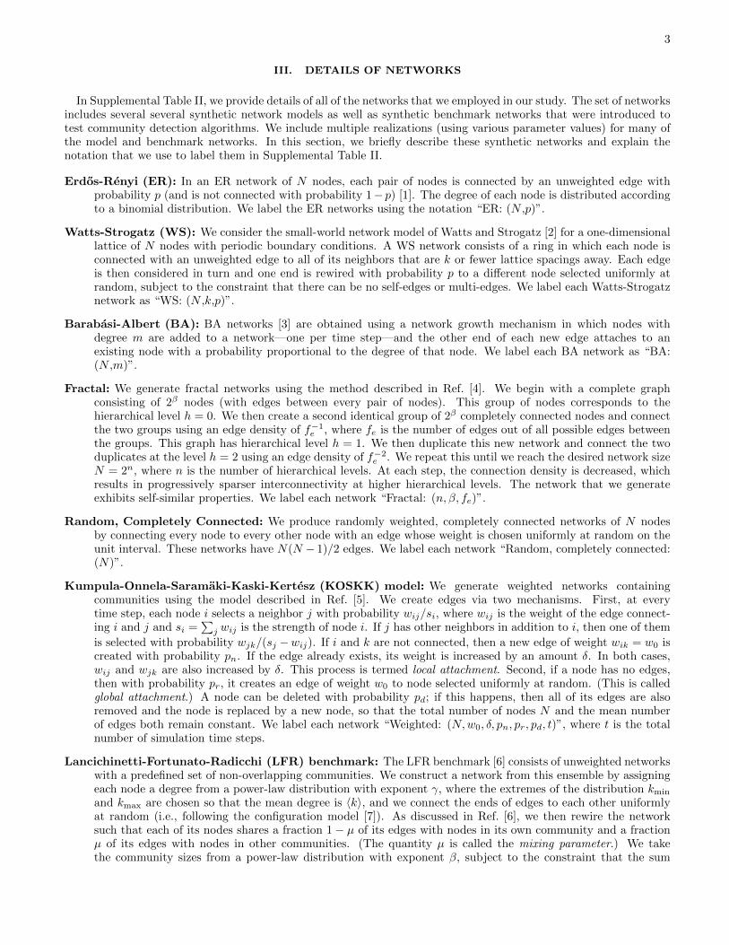
3
III. DETAILS OF NETWORKS
In Supplemental Table II, we provide details of all of the networks that we employed in our study. The set of networksincludes several several synthetic network models as well as synthetic benchmark networks that were introduced totest community detection algorithms. We include multiple realizations (using various parameter values) for many ofthe model and benchmark networks. In this section, we briefly describe these synthetic networks and explain thenotation that we use to label them in Supplemental Table II.
Erdos-Renyi (ER): In an ER network of N nodes, each pair of nodes is connected by an unweighted edge withprobability p (and is not connected with probability 1− p) [1]. The degree of each node is distributed accordingto a binomial distribution. We label the ER networks using the notation “ER: (N ,p)”.
Watts-Strogatz (WS): We consider the small-world network model of Watts and Strogatz [2] for a one-dimensionallattice of N nodes with periodic boundary conditions. A WS network consists of a ring in which each node isconnected with an unweighted edge to all of its neighbors that are k or fewer lattice spacings away. Each edgeis then considered in turn and one end is rewired with probability p to a different node selected uniformly atrandom, subject to the constraint that there can be no self-edges or multi-edges. We label each Watts-Strogatznetwork as “WS: (N ,k,p)”.
Barabasi-Albert (BA): BA networks [3] are obtained using a network growth mechanism in which nodes withdegree m are added to a network—one per time step—and the other end of each new edge attaches to anexisting node with a probability proportional to the degree of that node. We label each BA network as “BA:(N ,m)”.
Fractal: We generate fractal networks using the method described in Ref. [4]. We begin with a complete graphconsisting of 2β nodes (with edges between every pair of nodes). This group of nodes corresponds to thehierarchical level h = 0. We then create a second identical group of 2β completely connected nodes and connectthe two groups using an edge density of f−1
e , where fe is the number of edges out of all possible edges betweenthe groups. This graph has hierarchical level h = 1. We then duplicate this new network and connect the twoduplicates at the level h = 2 using an edge density of f−2
e . We repeat this until we reach the desired network sizeN = 2n, where n is the number of hierarchical levels. At each step, the connection density is decreased, whichresults in progressively sparser interconnectivity at higher hierarchical levels. The network that we generateexhibits self-similar properties. We label each network “Fractal: (n,β, fe)”.
Random, Completely Connected: We produce randomly weighted, completely connected networks of N nodesby connecting every node to every other node with an edge whose weight is chosen uniformly at random on theunit interval. These networks have N(N − 1)/2 edges. We label each network “Random, completely connected:(N)”.
Kumpula-Onnela-Saramaki-Kaski-Kertesz (KOSKK) model: We generate weighted networks containingcommunities using the model described in Ref. [5]. We create edges via two mechanisms. First, at everytime step, each node i selects a neighbor j with probability wij/si, where wij is the weight of the edge connect-ing i and j and si =
�j wij is the strength of node i. If j has other neighbors in addition to i, then one of them
is selected with probability wjk/(sj −wij). If i and k are not connected, then a new edge of weight wik = w0 iscreated with probability pn. If the edge already exists, its weight is increased by an amount δ. In both cases,wij and wjk are also increased by δ. This process is termed local attachment. Second, if a node has no edges,then with probability pr, it creates an edge of weight w0 to node selected uniformly at random. (This is calledglobal attachment.) A node can be deleted with probability pd; if this happens, then all of its edges are alsoremoved and the node is replaced by a new node, so that the total number of nodes N and the mean numberof edges both remain constant. We label each network “Weighted: (N,w0, δ, pn, pr, pd, t)”, where t is the totalnumber of simulation time steps.
Lancichinetti-Fortunato-Radicchi (LFR) benchmark: The LFR benchmark [6] consists of unweighted networkswith a predefined set of non-overlapping communities. We construct a network from this ensemble by assigningeach node a degree from a power-law distribution with exponent γ, where the extremes of the distribution kmin
and kmax are chosen so that the mean degree is �k�, and we connect the ends of edges to each other uniformlyat random (i.e., following the configuration model [7]). As discussed in Ref. [6], we then rewire the networksuch that each of its nodes shares a fraction 1− µ of its edges with nodes in its own community and a fractionµ of its edges with nodes in other communities. (The quantity µ is called the mixing parameter.) We takethe community sizes from a power-law distribution with exponent β, subject to the constraint that the sum

4
of all of the community sizes equals the number of nodes N in the network. We choose the minimum andmaximum community sizes (qmin and qmax) so that they satisfy the additional constraint that qmin > kmin andqmax > kmax; this ensures that each node is included in at least one community. We label each network “LFR:(N, �k�, kmax, γ,β, µ, qmin, qmax)”.
Lancichinetti-Fortunato (LF) benchmark: The LF benchmark [8] allows networks to be weighted and to haveoverlapping communities. In the present paper, we only consider weighted networks with non-overlappingcommunities. We again take the node degrees from a power-law degree distribution (as in LFR benchmarknetworks), but this time we label the exponent τ1, and we take the community sizes from a power-law degreedistribution with exponent τ2. The strength si of each node is chosen so that si = kβi , where ki again gives thedegree of node i. As discussed at length in Ref. [8], there are also two mixing parameters: the topological mixingparameter µt specifies the proportion of edges that connect nodes in different communities; and the participationmixing parameter µw specifies the fraction of the total edge weight between nodes from different communities.We label each network “LF: (N, �k�, kmax, µt, µw,β, τ1, τ2)”. For all of the LF networks, we set N = 1000. Onecan alternatively set the minimum and maximum community sizes qmin and qmax. We always use qmin = 20 andqmax = 50, so we do not include these parameters when we label the networks.
LF-Newman-Girvan benchmark: We include an LF network ensemble with parameters values N = 128, �k� = 16,kmax = 16, µt = 0.1, µw = 0.1, qmin = 32, qmax = 32, and β = 1. This family of networks is similar to the NGbenchmark [8, 9].
IV. SUPPLEMENTAL TABLE II

5
TABLE II. Network summary statistics. We symmetrize all networks, remove self-edges, and only consider largest connectedcomponents. In this table, we give the network category, whether it is weighted or unweighted, the number of nodes Nin the largest connected component, the number of edges L in this component, the fraction of possible edges present ed =2L/[N(N − 1)], and a reference providing details of the data source. We highlight the 25 networks used in the randomizationsin Appendix A in bold and the 189 networks used in the aggregate taxonomy in red. We indicate with an asterisk (∗) allnetworks used in Appendix B to test the robustness of the taxonomy to different optimization heuristics.
ID Name Category Weighted N L ed References
1 Human brain cortex: participant A1 Brain Y 994 13,520 0.0274 [10]
2 Human brain cortex: participant A2 Brain Y 987 14,865 0.0305 [10]
3 Human brain cortex: participant B Brain Y 980 14,222 0.0296 [10]
4 Human brain cortex: participant D Brain Y 996 14,851 0.0300 [10]
5 Human brain cortex: participant E Brain Y 992 14,372 0.0292 [10]
6 Human brain cortex: participant C Brain Y 996 14,933 0.0301 [10]
7 Cat brain: cortical∗ Brain Y 52 515 0.3884 [11]
8 Cat brain: cortical/thalmic∗ Brain Y 95 1,170 0.2620 [11]
9 Macaque brain: cortical∗ Brain N 47 313 0.2895 [12]
10 Macaque brain: visual/sensory cortex∗ Brain N 71 438 0.1763 [12]
11 Macaque brain: visual cortex 1∗ Brain N 30 190 0.4368 [13]
12 Macaque brain: visual cortex 2∗ Brain N 32 194 0.3911 [13]
13 Coauthorship: astrophysics Collaboration Y 14,845 119,652 0.0011 [14]
14 Coauthorship: comp. geometry Collaboration Y 3,621 9,461 0.0014 [15, 16]
15 Coauthorship: condensed matter Collaboration Y 13,861 44,619 0.0005 [14]
16 Coauthorship: Erdos Collaboration N 6,927 11,850 0.0005 [17]
17 Coauthorship: high-energy theory Collaboration Y 5,835 13,815 0.0008 [14]
18 Coauthorship: network science Collaboration Y 379 914 0.0128 [18]
19 Hollywood film music∗ Collaboration Y 39 219 0.2955 [19]
20 Jazz collaboration Collaboration N 198 2,742 0.1406 [20]
21 Facebook: American Facebook N 6,370 217,654 0.0107 [21, 22]
22 Facebook: Amherst Facebook N 2,235 90,954 0.0364 [21, 22]
23 Facebook: Auburn Facebook N 18,448 973,918 0.0057 [21, 22]
24 Facebook: Baylor Facebook N 12,799 679,815 0.0083 [21, 22]
25 Facebook: BC Facebook N 11,498 486,961 0.0074 [21, 22]
26 Facebook: Berkeley Facebook N 22,900 852,419 0.0033 [21, 22]
27 Facebook: Bingham Facebook N 10,001 362,892 0.0073 [21, 22]
28 Facebook: Bowdoin Facebook N 2,250 84,386 0.0334 [21, 22]
29 Facebook: Brandeis Facebook N 3,887 137,561 0.0182 [21, 22]
30 Facebook: Brown Facebook N 8,586 384,519 0.0104 [21, 22]
31 Facebook: BU Facebook N 19,666 637,509 0.0033 [21, 22]
32 Facebook: Bucknell Facebook N 3,824 158,863 0.0217 [21, 22]
33 Facebook: Cal Facebook N 11,243 351,356 0.0056 [21, 22]
34 Facebook: Caltech Facebook N 762 16,651 0.0574 [21, 22]
35 Facebook: Carnegie Facebook N 6,621 249,959 0.0114 [21, 22]
36 Facebook: Colgate Facebook N 3,482 155,043 0.0256 [21, 22]
37 Facebook: Columbia Facebook N 11,706 444,295 0.0065 [21, 22]
38 Facebook: Cornell Facebook N 18,621 790,753 0.0046 [21, 22]
39 Facebook: Dartmouth Facebook N 7,677 304,065 0.0103 [21, 22]
40 Facebook: Duke Facebook N 9,885 506,437 0.0104 [21, 22]
41 Facebook: Emory Facebook N 7,449 330,008 0.0119 [21, 22]
42 Facebook: FSU Facebook N 27,731 1,034,799 0.0027 [21, 22]
43 Facebook: Georgetown Facebook N 9,388 425,619 0.0097 [21, 22]
44 Facebook: GWU Facebook N 12,164 469,511 0.0063 [21, 22]
45 Facebook: Hamilton Facebook N 2,312 96,393 0.0361 [21, 22]
46 Facebook: Harvard Facebook N 15,086 824,595 0.0072 [21, 22]
47 Facebook: Haverford Facebook N 1,446 59,589 0.0570 [21, 22]
48 Facebook: Howard Facebook N 4,047 204,850 0.0250 [21, 22]
49 Facebook: Indiana Facebook N 29,732 1,305,757 0.0030 [21, 22]
50 Facebook: JMU Facebook N 14,070 485,564 0.0049 [21, 22]

6
TABLE II. (Continued.)
ID Name Category Weighted N L ed References
51 Facebook: Johns Facebook N 5,157 186,572 0.0140 [21, 22]
52 Facebook: Lehigh Facebook N 5,073 198,346 0.0154 [21, 22]
53 Facebook: Maine Facebook N 9,065 243,245 0.0059 [21, 22]
54 Facebook: Maryland Facebook N 20,829 744,832 0.0034 [21, 22]
55 Facebook: Mich Facebook N 3,745 81,901 0.0117 [21, 22]
56 Facebook: Michigan Facebook N 30,106 1,176,489 0.0026 [21, 22]
57 Facebook: Middlebury Facebook N 3,069 124,607 0.0265 [21, 22]
58 Facebook: Mississippi Facebook N 10,519 610,910 0.0110 [21, 22]
59 Facebook: MIT Facebook N 6,402 251,230 0.0123 [21, 22]
60 Facebook: MSU Facebook N 32,361 1,118,767 0.0021 [21, 22]
61 Facebook: MU Facebook N 15,425 649,441 0.0055 [21, 22]
62 Facebook: Northeastern Facebook N 13,868 381,919 0.0040 [21, 22]
63 Facebook: Northwestern Facebook N 10,537 488,318 0.0088 [21, 22]
64 Facebook: Notre Dame Facebook N 12,149 541,336 0.0073 [21, 22]
65 Facebook: NYU Facebook Y 21,623 715,673 0.0031 [21, 22]
66 Facebook: Oberlin Facebook N 2,920 89,912 0.0211 [21, 22]
67 Facebook: Oklahoma Facebook N 17,420 892,524 0.0059 [21, 22]
68 Facebook: Penn Facebook N 41,536 1,362,220 0.0016 [21, 22]
69 Facebook: Pepperdine Facebook N 3,440 152,003 0.0257 [21, 22]
70 Facebook: Princeton Facebook N 6,575 293,307 0.0136 [21, 22]
71 Facebook: Reed Facebook N 962 18,812 0.0407 [21, 22]
72 Facebook: Rice Facebook N 4,083 184,826 0.0222 [21, 22]
73 Facebook: Rochester Facebook N 4,561 161,403 0.0155 [21, 22]
74 Facebook: Rutgers Facebook N 24,568 784,596 0.0026 [21, 22]
75 Facebook: Santa Facebook N 3,578 151,747 0.0237 [21, 22]
76 Facebook: Simmons Facebook N 1,510 32,984 0.0290 [21, 22]
77 Facebook: Smith Facebook N 2,970 97,133 0.0220 [21, 22]
78 Facebook: Stanford Facebook N 11,586 568,309 0.0085 [21, 22]
79 Facebook: Swarthmore Facebook N 1,657 61,049 0.0445 [21, 22]
80 Facebook: Syracuse Facebook N 13,640 543,975 0.0058 [21, 22]
81 Facebook: Temple Facebook N 13,653 360,774 0.0039 [21, 22]
82 Facebook: Tennessee Facebook N 16,977 770,658 0.0053 [21, 22]
83 Facebook: Texas80 Facebook N 31,538 1,219,639 0.0025 [21, 22]
84 Facebook: Texas84 Facebook N 36,364 1,590,651 0.0024 [21, 22]
85 Facebook: Trinity Facebook N 2,613 111,996 0.0328 [21, 22]
86 Facebook: Tufts Facebook N 6,672 249,722 0.0112 [21, 22]
87 Facebook: Tulane Facebook N 7,740 283,912 0.0095 [21, 22]
88 Facebook: U. Chicago Facebook N 6,561 208,088 0.0097 [21, 22]
89 Facebook: U. Conn. Facebook N 17,206 604,867 0.0041 [21, 22]
90 Facebook: U. Illinois Facebook N 30,795 1,264,421 0.0027 [21, 22]
91 Facebook: U. Mass. Facebook N 16,502 519,376 0.0038 [21, 22]
92 Facebook: U. Penn. Facebook N 14,888 686,485 0.0062 [21, 22]
93 Facebook: UC33 Facebook N 16,800 522,141 0.0037 [21, 22]
94 Facebook: UC61 Facebook N 13,736 442,169 0.0047 [21, 22]
95 Facebook: UC64 Facebook N 6,810 155,320 0.0067 [21, 22]
96 Facebook: UCF Facebook N 14,936 428,987 0.0038 [21, 22]
97 Facebook: UCLA Facebook N 20,453 747,604 0.0036 [21, 22]
98 Facebook: UCSB Facebook N 14,917 482,215 0.0043 [21, 22]
99 Facebook: UCSC Facebook N 8,979 224,578 0.0056 [21, 22]
100 Facebook: UCSD Facebook N 14,936 443,215 0.0040 [21, 22]

7
TABLE II. (Continued.)
ID Name Category Weighted N L ed References
101 Facebook: UF Facebook N 35,111 1,465,654 0.0024 [21, 22]
102 Facebook: UGA Facebook N 24,380 1,174,051 0.0040 [21, 22]
103 Facebook: UNC Facebook N 18,158 766,796 0.0047 [21, 22]
104 Facebook: USC Facebook N 17,440 801,851 0.0053 [21, 22]
105 Facebook: USF Facebook N 13,367 321,209 0.0036 [21, 22]
106 Facebook: USFCA Facebook N 2,672 65,244 0.0183 [21, 22]
107 Facebook: UVA Facebook N 17,178 789,308 0.0054 [21, 22]
108 Facebook: Vanderbilt Facebook N 8,063 427,829 0.0132 [21, 22]
109 Facebook: Vassar Facebook N 3,068 119,161 0.0253 [21, 22]
110 Facebook: Vermont Facebook N 7,322 191,220 0.0071 [21, 22]
111 Facebook: Villanova Facebook N 7,755 314,980 0.0105 [21, 22]
112 Facebook: Virginia Facebook N 21,319 698,175 0.0031 [21, 22]
113 Facebook: Wake Facebook N 5,366 279,186 0.0194 [21, 22]
114 Facebook: Wash. U. Facebook N 7,730 367,526 0.0123 [21, 22]
115 Facebook: Wellesley Facebook N 2,970 94,899 0.0215 [21, 22]
116 Facebook: Wesleyan Facebook N 3,591 138,034 0.0214 [21, 22]
117 Facebook: William Facebook N 6,472 266,378 0.0127 [21, 22]
118 Facebook: Williams Facebook N 2,788 112,985 0.0291 [21, 22]
119 Facebook: Wisconsin Facebook N 23,831 835,946 0.0029 [21, 22]
120 Facebook: Yale Facebook N 8,561 405,440 0.0111 [21, 22]
121 NYSE: 1980–1999 Financial Y 477 113,526 1.0000 [23]
122 NYSE: 1980–1983 Financial Y 477 113,526 1.0000 [23]
123 NYSE: 1984–1987 Financial Y 477 113,526 1.0000 [23]
124 NYSE: 1988–1991 Financial Y 477 113,526 1.0000 [23]
125 NYSE: 1992–1995 Financial Y 477 113,526 1.0000 [23]
126 NYSE: 1996–1999 Financial Y 477 113,526 1.0000 [23]
127 NYSE: H1 1985 Financial Y 100 4,950 1.0000 [24]
128 NYSE: H2 1985 Financial Y 100 4,950 1.0000 [24]
129 NYSE: H1 1986 Financial Y 100 4,950 1.0000 [24]
130 NYSE: H2 1986 Financial Y 100 4,950 1.0000 [24]
131 NYSE: H1 1987 Financial Y 100 4,950 1.0000 [24]
132 NYSE: H2 1987 Financial Y 100 4,950 1.0000 [24]
133 NYSE: H1 1988 Financial Y 100 4,950 1.0000 [24]
134 NYSE: H2 1988 Financial Y 100 4,950 1.0000 [24]
135 NYSE: H1 1989 Financial Y 100 4,950 1.0000 [24]
136 NYSE: H2 1989 Financial Y 100 4,950 1.0000 [24]
137 NYSE: H1 1990 Financial Y 100 4,950 1.0000 [24]
138 NYSE: H2 1990 Financial Y 100 4,950 1.0000 [24]
139 NYSE: H1 1991 Financial Y 100 4,950 1.0000 [24]
140 NYSE: H2 1991 Financial Y 100 4,950 1.0000 [24]
141 NYSE: H1 1992 Financial Y 100 4,950 1.0000 [24]
142 NYSE: H2 1992 Financial Y 100 4,950 1.0000 [24]
143 NYSE: H1 1993 Financial Y 100 4,950 1.0000 [24]
144 NYSE: H2 1993 Financial Y 100 4,950 1.0000 [24]
145 NYSE: H1 1994 Financial Y 100 4,950 1.0000 [24]
146 NYSE: H2 1994 Financial Y 100 4,950 1.0000 [24]
147 NYSE: H1 1995 Financial Y 100 4,950 1.0000 [24]
148 NYSE: H2 1995 Financial Y 100 4,950 1.0000 [24]
149 NYSE: H1 1996 Financial Y 100 4,950 1.0000 [24]
150 NYSE: H2 1996 Financial Y 100 4,950 1.0000 [24]
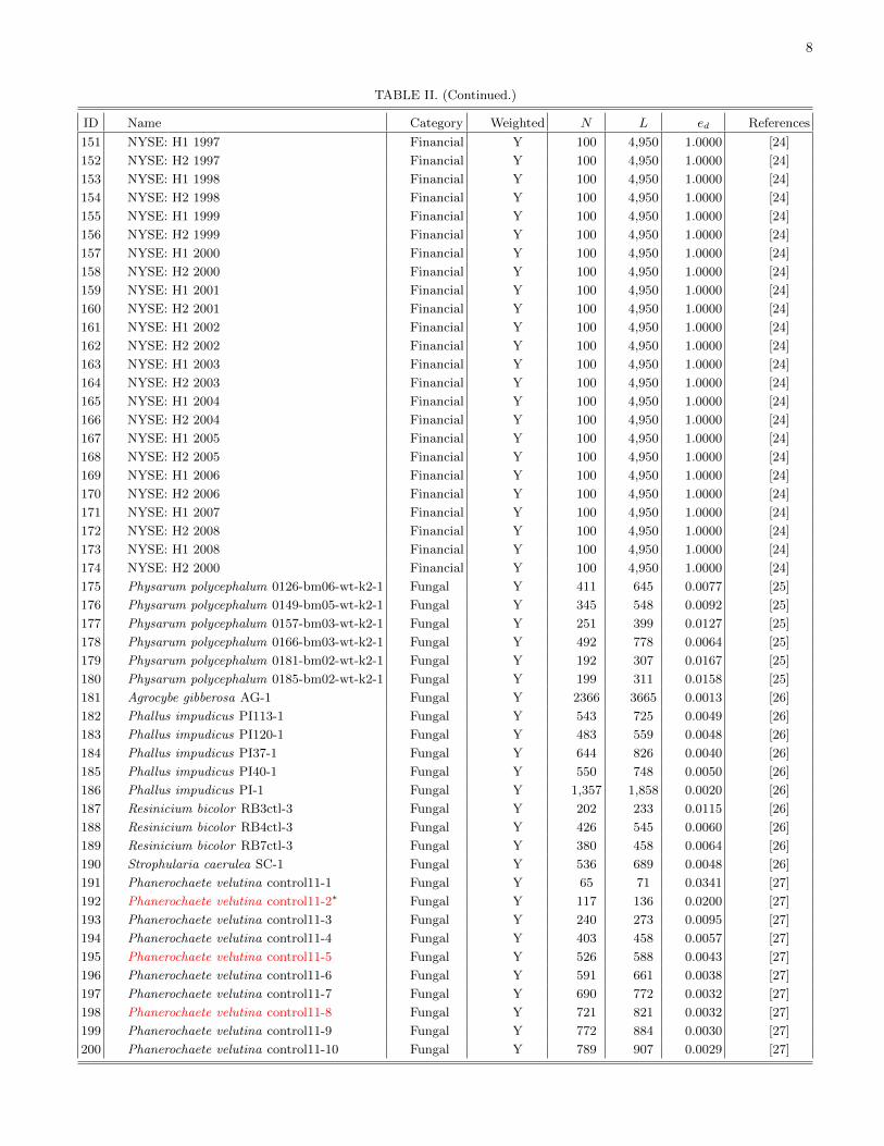
8
TABLE II. (Continued.)
ID Name Category Weighted N L ed References
151 NYSE: H1 1997 Financial Y 100 4,950 1.0000 [24]
152 NYSE: H2 1997 Financial Y 100 4,950 1.0000 [24]
153 NYSE: H1 1998 Financial Y 100 4,950 1.0000 [24]
154 NYSE: H2 1998 Financial Y 100 4,950 1.0000 [24]
155 NYSE: H1 1999 Financial Y 100 4,950 1.0000 [24]
156 NYSE: H2 1999 Financial Y 100 4,950 1.0000 [24]
157 NYSE: H1 2000 Financial Y 100 4,950 1.0000 [24]
158 NYSE: H2 2000 Financial Y 100 4,950 1.0000 [24]
159 NYSE: H1 2001 Financial Y 100 4,950 1.0000 [24]
160 NYSE: H2 2001 Financial Y 100 4,950 1.0000 [24]
161 NYSE: H1 2002 Financial Y 100 4,950 1.0000 [24]
162 NYSE: H2 2002 Financial Y 100 4,950 1.0000 [24]
163 NYSE: H1 2003 Financial Y 100 4,950 1.0000 [24]
164 NYSE: H2 2003 Financial Y 100 4,950 1.0000 [24]
165 NYSE: H1 2004 Financial Y 100 4,950 1.0000 [24]
166 NYSE: H2 2004 Financial Y 100 4,950 1.0000 [24]
167 NYSE: H1 2005 Financial Y 100 4,950 1.0000 [24]
168 NYSE: H2 2005 Financial Y 100 4,950 1.0000 [24]
169 NYSE: H1 2006 Financial Y 100 4,950 1.0000 [24]
170 NYSE: H2 2006 Financial Y 100 4,950 1.0000 [24]
171 NYSE: H1 2007 Financial Y 100 4,950 1.0000 [24]
172 NYSE: H2 2008 Financial Y 100 4,950 1.0000 [24]
173 NYSE: H1 2008 Financial Y 100 4,950 1.0000 [24]
174 NYSE: H2 2000 Financial Y 100 4,950 1.0000 [24]
175 Physarum polycephalum 0126-bm06-wt-k2-1 Fungal Y 411 645 0.0077 [25]
176 Physarum polycephalum 0149-bm05-wt-k2-1 Fungal Y 345 548 0.0092 [25]
177 Physarum polycephalum 0157-bm03-wt-k2-1 Fungal Y 251 399 0.0127 [25]
178 Physarum polycephalum 0166-bm03-wt-k2-1 Fungal Y 492 778 0.0064 [25]
179 Physarum polycephalum 0181-bm02-wt-k2-1 Fungal Y 192 307 0.0167 [25]
180 Physarum polycephalum 0185-bm02-wt-k2-1 Fungal Y 199 311 0.0158 [25]
181 Agrocybe gibberosa AG-1 Fungal Y 2366 3665 0.0013 [26]
182 Phallus impudicus PI113-1 Fungal Y 543 725 0.0049 [26]
183 Phallus impudicus PI120-1 Fungal Y 483 559 0.0048 [26]
184 Phallus impudicus PI37-1 Fungal Y 644 826 0.0040 [26]
185 Phallus impudicus PI40-1 Fungal Y 550 748 0.0050 [26]
186 Phallus impudicus PI-1 Fungal Y 1,357 1,858 0.0020 [26]
187 Resinicium bicolor RB3ctl-3 Fungal Y 202 233 0.0115 [26]
188 Resinicium bicolor RB4ctl-3 Fungal Y 426 545 0.0060 [26]
189 Resinicium bicolor RB7ctl-3 Fungal Y 380 458 0.0064 [26]
190 Strophularia caerulea SC-1 Fungal Y 536 689 0.0048 [26]
191 Phanerochaete velutina control11-1 Fungal Y 65 71 0.0341 [27]
192 Phanerochaete velutina control11-2∗ Fungal Y 117 136 0.0200 [27]
193 Phanerochaete velutina control11-3 Fungal Y 240 273 0.0095 [27]
194 Phanerochaete velutina control11-4 Fungal Y 403 458 0.0057 [27]
195 Phanerochaete velutina control11-5 Fungal Y 526 588 0.0043 [27]
196 Phanerochaete velutina control11-6 Fungal Y 591 661 0.0038 [27]
197 Phanerochaete velutina control11-7 Fungal Y 690 772 0.0032 [27]
198 Phanerochaete velutina control11-8 Fungal Y 721 821 0.0032 [27]
199 Phanerochaete velutina control11-9 Fungal Y 772 884 0.0030 [27]
200 Phanerochaete velutina control11-10 Fungal Y 789 907 0.0029 [27]

9
TABLE II. (Continued.)
ID Name Category Weighted N L ed References
201 Phanerochaete velutina control11-11 Fungal Y 823 954 0.0028 [27]
202 Phanerochaete velutina control17-1 Fungal Y 16 15 0.1250 [27]
203 Phanerochaete velutina control17-2 Fungal Y 232 240 0.0090 [27]
204 Phanerochaete velutina control17-3 Fungal Y 502 539 0.0043 [27]
205 Phanerochaete velutina control17-4 Fungal Y 703 754 0.0031 [27]
206 Phanerochaete velutina control17-5 Fungal Y 816 874 0.0026 [27]
207 Phanerochaete velutina control17-6 Fungal Y 950 1,058 0.0023 [27]
208 Phanerochaete velutina control17-7 Fungal Y 1,047 1,182 0.0022 [27]
209 Phanerochaete velutina control17-8 Fungal Y 1,113 1,303 0.0021 [27]
210 Phanerochaete velutina control17-9 Fungal Y 1,142 1,347 0.0021 [27]
211 Phanerochaete velutina control17-10 Fungal Y 1,160 1,384 0.0021 [27]
212 Phanerochaete velutina control17-11 Fungal Y 1,205 1,469 0.0020 [27]
213 Phanerochaete velutina control4-1 Fungal Y 200 213 0.0107 [27]
214 Phanerochaete velutina control4-2 Fungal Y 461 490 0.0046 [27]
215 Phanerochaete velutina control4-3 Fungal Y 826 862 0.0025 [27]
216 Phanerochaete velutina control4-4 Fungal Y 1,044 1,087 0.0020 [27]
217 Phanerochaete velutina control4-5 Fungal Y 1,380 1,476 0.0016 [27]
218 Phanerochaete velutina control4-6 Fungal Y 1,623 1,767 0.0013 [27]
219 Phanerochaete velutina control4-7 Fungal Y 1,756 1,923 0.0012 [27]
220 Phanerochaete velutina control4-8 Fungal Y 1,869 2,061 0.0012 [27]
221 Phanerochaete velutina control4-9 Fungal Y 1,992 2,196 0.0011 [27]
222 Phanerochaete velutina control4-10 Fungal Y 2,086 2,301 0.0011 [27]
223 Phanerochaete velutina control4-11 Fungal Y 2,190 2,431 0.0010 [27]
224 Phallus impudicus pi150ctl-1 Fungal Y 1,810 2,537 0.0015 [26]
225 Phanerochaete velutina pv81-1 Fungal Y 75 82 0.0295 [28]
226 Phanerochaete velutina pv81-2 Fungal Y 653 897 0.0042 [28]
227 Phanerochaete velutina pv81-3 Fungal Y 911 1,255 0.0030 [28]
228 Phanerochaete velutina pv81-4 Fungal Y 1,064 1,467 0.0026 [28]
229 Phanerochaete velutina pv81-5 Fungal Y 986 1,351 0.0028 [28]
230 Phanerochaete velutina pv82-1 Fungal Y 111 112 0.0183 [28]
231 Phanerochaete velutina pv82-2 Fungal Y 467 523 0.0048 [28]
232 Phanerochaete velutina pv82-3 Fungal Y 630 726 0.0037 [28]
233 Phanerochaete velutina pv82-4 Fungal Y 644 749 0.0036 [28]
234 Phanerochaete velutina pv82-5 Fungal Y 551 627 0.0041 [28]
235 Phanerochaete velutina pv83-1 Fungal Y 129 142 0.0172 [28]
236 Phanerochaete velutina pv83-2 Fungal Y 424 510 0.0057 [28]
237 Phanerochaete velutina pv83-3 Fungal Y 671 857 0.0038 [28]
238 Phanerochaete velutina pv83-4 Fungal Y 708 905 0.0036 [28]
239 Phanerochaete velutina pv83-5 Fungal Y 551 668 0.0044 [28]
240 Online Dictionary of Computing Language Y 13,356 91,471 0.0010 [29]
241 Online Dictionary Of Information Science Language Y 2,898 16,376 0.0039 [16, 30]
242 Reuters 9/11 news Language Y 13,308 148,035 0.0017 [31]
243 Roget’s thesaurus Language N 994 3,640 0.0074 [16, 32]
244 Word adjacency: English Language N 7,377 44,205 0.0016 [33]
245 Word adjacency: French Language N 8,308 23,832 0.0007 [33]
246 Word adjacency: Japanese Language N 2,698 7,995 0.0022 [33]
247 Word adjacency: Spanish Language N 11,558 43,050 0.0006 [33]
248 Metabolic: AA Metabolic N 411 1,818 0.0216 [34]
249 Metabolic: AB Metabolic N 386 1,691 0.0228 [34]
250 Metabolic: AG Metabolic N 494 2,173 0.0178 [34]
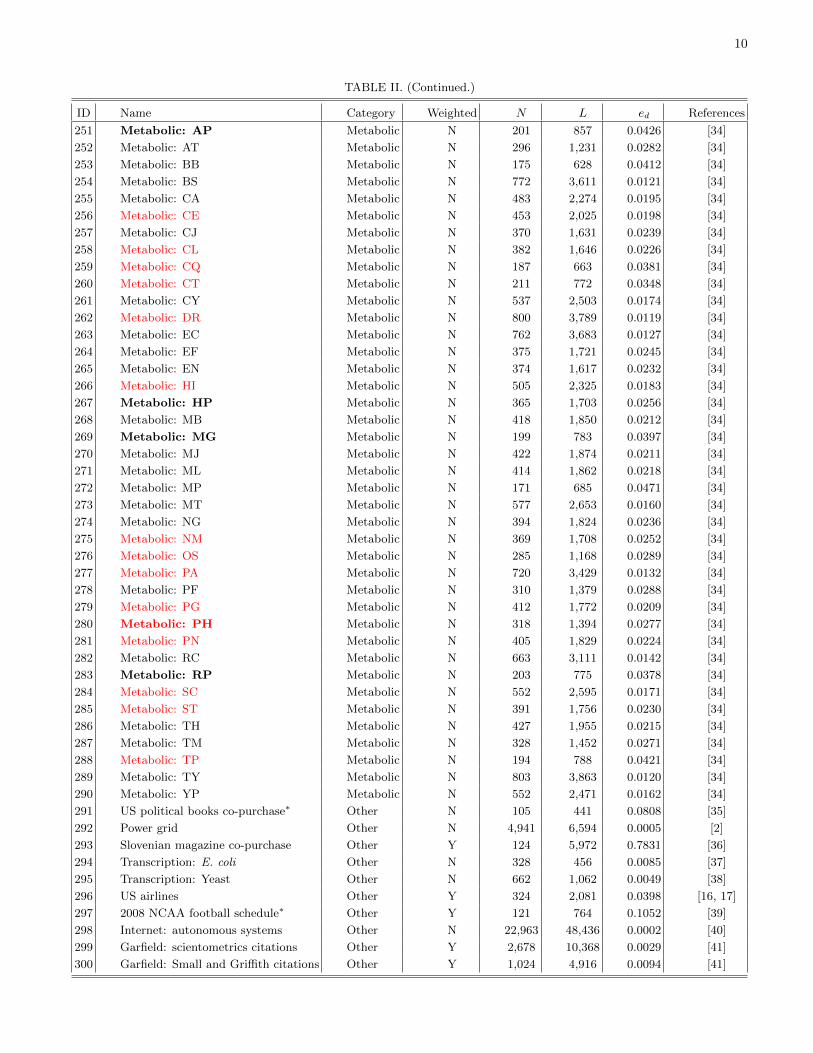
10
TABLE II. (Continued.)
ID Name Category Weighted N L ed References
251 Metabolic: AP Metabolic N 201 857 0.0426 [34]
252 Metabolic: AT Metabolic N 296 1,231 0.0282 [34]
253 Metabolic: BB Metabolic N 175 628 0.0412 [34]
254 Metabolic: BS Metabolic N 772 3,611 0.0121 [34]
255 Metabolic: CA Metabolic N 483 2,274 0.0195 [34]
256 Metabolic: CE Metabolic N 453 2,025 0.0198 [34]
257 Metabolic: CJ Metabolic N 370 1,631 0.0239 [34]
258 Metabolic: CL Metabolic N 382 1,646 0.0226 [34]
259 Metabolic: CQ Metabolic N 187 663 0.0381 [34]
260 Metabolic: CT Metabolic N 211 772 0.0348 [34]
261 Metabolic: CY Metabolic N 537 2,503 0.0174 [34]
262 Metabolic: DR Metabolic N 800 3,789 0.0119 [34]
263 Metabolic: EC Metabolic N 762 3,683 0.0127 [34]
264 Metabolic: EF Metabolic N 375 1,721 0.0245 [34]
265 Metabolic: EN Metabolic N 374 1,617 0.0232 [34]
266 Metabolic: HI Metabolic N 505 2,325 0.0183 [34]
267 Metabolic: HP Metabolic N 365 1,703 0.0256 [34]
268 Metabolic: MB Metabolic N 418 1,850 0.0212 [34]
269 Metabolic: MG Metabolic N 199 783 0.0397 [34]
270 Metabolic: MJ Metabolic N 422 1,874 0.0211 [34]
271 Metabolic: ML Metabolic N 414 1,862 0.0218 [34]
272 Metabolic: MP Metabolic N 171 685 0.0471 [34]
273 Metabolic: MT Metabolic N 577 2,653 0.0160 [34]
274 Metabolic: NG Metabolic N 394 1,824 0.0236 [34]
275 Metabolic: NM Metabolic N 369 1,708 0.0252 [34]
276 Metabolic: OS Metabolic N 285 1,168 0.0289 [34]
277 Metabolic: PA Metabolic N 720 3,429 0.0132 [34]
278 Metabolic: PF Metabolic N 310 1,379 0.0288 [34]
279 Metabolic: PG Metabolic N 412 1,772 0.0209 [34]
280 Metabolic: PH Metabolic N 318 1,394 0.0277 [34]
281 Metabolic: PN Metabolic N 405 1,829 0.0224 [34]
282 Metabolic: RC Metabolic N 663 3,111 0.0142 [34]
283 Metabolic: RP Metabolic N 203 775 0.0378 [34]
284 Metabolic: SC Metabolic N 552 2,595 0.0171 [34]
285 Metabolic: ST Metabolic N 391 1,756 0.0230 [34]
286 Metabolic: TH Metabolic N 427 1,955 0.0215 [34]
287 Metabolic: TM Metabolic N 328 1,452 0.0271 [34]
288 Metabolic: TP Metabolic N 194 788 0.0421 [34]
289 Metabolic: TY Metabolic N 803 3,863 0.0120 [34]
290 Metabolic: YP Metabolic N 552 2,471 0.0162 [34]
291 US political books co-purchase∗ Other N 105 441 0.0808 [35]
292 Power grid Other N 4,941 6,594 0.0005 [2]
293 Slovenian magazine co-purchase Other Y 124 5,972 0.7831 [36]
294 Transcription: E. coli Other N 328 456 0.0085 [37]
295 Transcription: Yeast Other N 662 1,062 0.0049 [38]
296 US airlines Other Y 324 2,081 0.0398 [16, 17]
297 2008 NCAA football schedule∗ Other Y 121 764 0.1052 [39]
298 Internet: autonomous systems Other N 22,963 48,436 0.0002 [40]
299 Garfield: scientometrics citations Other Y 2,678 10,368 0.0029 [41]
300 Garfield: Small and Griffith citations Other Y 1,024 4,916 0.0094 [41]

11
TABLE II. (Continued.)
ID Name Category Weighted N L ed References
301 Garfield: small-world citations Other N 233 994 0.0368 [41]
302 Electronic circuit (s208)∗ Other N 122 189 0.0256 [33]
303 Electronic circuit (s420) Other N 252 399 0.0126 [33]
304 Electronic circuit (s838) Other N 512 819 0.0063 [33]
305 Protein: serine protease inhibitor (1EAW)∗ Other N 53 123 0.0893 [33]
306 Protein: immunoglobulin (1A4J)∗ Other N 95 213 0.0477 [33]
307 Protein: oxidoreductase (1AOR)∗ Other N 97 212 0.0455 [33]
308 AIDS blogs∗ Other N 146 180 0.0170 [42]
309 Political blogs Other Y 1,222 16,714 0.0224 [43]
310 WWW (Stanford) Other N 8,929 26,320 0.0007 [44]
311 Trade product proximity Other Y 775 283,094 0.9439 [45]
312 World trade in metal (1994): Net Other Y 80 875 0.2769 [16, 46]
313 World trade in metal (1994): Total Other Y 80 875 0.2769 [16, 46]
314 Bill cosponsorship: US House 96 Political: cosponsorship Y 438 95,529 0.9982 [47, 48]
315 Bill cosponsorship: US House 97 Political: cosponsorship Y 435 94,374 0.9998 [47, 48]
316 Bill cosponsorship: US House 98 Political: cosponsorship Y 437 95,256 0.9999 [47, 48]
317 Bill cosponsorship: US House 99 Political: cosponsorship Y 437 94,999 0.9972 [47, 48]
318 Bill cosponsorship: US House 100 Political: cosponsorship Y 439 96,125 0.9998 [47, 48]
319 Bill cosponsorship: US House 101 Political: cosponsorship Y 437 95,263 1.0000 [47, 48]
320 Bill cosponsorship: US House 102 Political: cosponsorship Y 437 95,051 0.9977 [47, 48]
321 Bill cosponsorship: US House 103 Political: cosponsorship Y 437 95,028 0.9975 [47, 48]
322 Bill cosponsorship: US House 104 Political: cosponsorship Y 439 95,925 0.9978 [47, 48]
323 Bill cosponsorship: US House 105 Political: cosponsorship Y 442 97,373 0.9991 [47, 48]
324 Bill cosponsorship: US House 106 Political: cosponsorship Y 436 94,820 0.9999 [47, 48]
325 Bill cosponsorship: US House 107 Political: cosponsorship Y 442 97,233 0.9977 [47, 48]
326 Bill cosponsorship: US House 108 Political: cosponsorship Y 439 96,104 0.9996 [47, 48]
327 Bill cosponsorship: US Senate 96 Political: cosponsorship Y 101 5,050 1.0000 [47, 48]
328 Bill cosponsorship: US Senate 97 Political: cosponsorship Y 101 5,050 1.0000 [47, 48]
329 Bill cosponsorship: US Senate 98 Political: cosponsorship Y 101 5,050 1.0000 [47, 48]
330 Bill cosponsorship: US Senate 99 Political: cosponsorship Y 101 5,049 0.9998 [47, 48]
331 Bill cosponsorship: US Senate 100 Political: cosponsorship Y 101 5,050 1.0000 [47, 48]
332 Bill cosponsorship: US Senate 101 Political: cosponsorship Y 100 4,950 1.0000 [47, 48]
333 Bill cosponsorship: US Senate 102 Political: cosponsorship Y 102 5,142 0.9983 [47, 48]
334 Bill cosponsorship: US Senate 103 Political: cosponsorship Y 101 5,050 1.0000 [47, 48]
335 Bill cosponsorship: US Senate 104 Political: cosponsorship Y 102 5,151 1.0000 [47, 48]
336 Bill cosponsorship: US Senate 105 Political: cosponsorship Y 100 4,950 1.0000 [47, 48]
337 Bill cosponsorship: US Senate 106 Political: cosponsorship Y 102 5,151 1.0000 [47, 48]
338 Bill cosponsorship: US Senate 107 Political: cosponsorship Y 101 5,049 0.9998 [47, 48]
339 Bill cosponsorship: US Senate 108 Political: cosponsorship Y 100 4,950 1.0000 [47, 48]
340 Committees: US House 101, comms. Political: committee N 159 3,610 0.2874 [49, 50]
341 Committees: US House 102, comms. Political: committee N 163 4,093 0.3100 [49, 50]
342 Committees: US House 103, comms. Political: committee N 141 2,983 0.3022 [49, 50]
343 Committees: US House 104, comms. Political: committee N 106 1,839 0.3305 [49, 50]
344 Committees: US House 105, comms. Political: committee N 108 1,997 0.3456 [49, 50]
345 Committees: US House 106, comms. Political: committee N 107 2,031 0.3581 [49, 50]
346 Committees: US House 107, comms. Political: committee N 113 2,429 0.3838 [49, 50]
347 Committees: US House 108, comms. Political: committee N 118 2,905 0.4208 [49, 50]
348 Committees: US House 101, Reps. Political: committee N 434 18,714 0.1992 [49, 50]
349 Committees: US House 102, Reps. Political: committee N 436 20,134 0.2123 [49, 50]
350 Committees: US House 103, Reps. Political: committee N 437 18,212 0.1912 [49, 50]
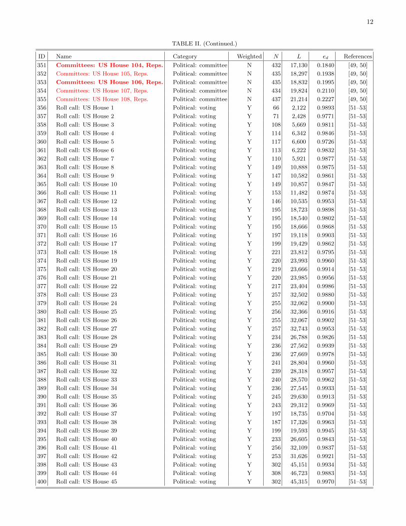
12
TABLE II. (Continued.)
ID Name Category Weighted N L ed References
351 Committees: US House 104, Reps. Political: committee N 432 17,130 0.1840 [49, 50]
352 Committees: US House 105, Reps. Political: committee N 435 18,297 0.1938 [49, 50]
353 Committees: US House 106, Reps. Political: committee N 435 18,832 0.1995 [49, 50]
354 Committees: US House 107, Reps. Political: committee N 434 19,824 0.2110 [49, 50]
355 Committees: US House 108, Reps. Political: committee N 437 21,214 0.2227 [49, 50]
356 Roll call: US House 1 Political: voting Y 66 2,122 0.9893 [51–53]
357 Roll call: US House 2 Political: voting Y 71 2,428 0.9771 [51–53]
358 Roll call: US House 3 Political: voting Y 108 5,669 0.9811 [51–53]
359 Roll call: US House 4 Political: voting Y 114 6,342 0.9846 [51–53]
360 Roll call: US House 5 Political: voting Y 117 6,600 0.9726 [51–53]
361 Roll call: US House 6 Political: voting Y 113 6,222 0.9832 [51–53]
362 Roll call: US House 7 Political: voting Y 110 5,921 0.9877 [51–53]
363 Roll call: US House 8 Political: voting Y 149 10,888 0.9875 [51–53]
364 Roll call: US House 9 Political: voting Y 147 10,582 0.9861 [51–53]
365 Roll call: US House 10 Political: voting Y 149 10,857 0.9847 [51–53]
366 Roll call: US House 11 Political: voting Y 153 11,482 0.9874 [51–53]
367 Roll call: US House 12 Political: voting Y 146 10,535 0.9953 [51–53]
368 Roll call: US House 13 Political: voting Y 195 18,723 0.9898 [51–53]
369 Roll call: US House 14 Political: voting Y 195 18,540 0.9802 [51–53]
370 Roll call: US House 15 Political: voting Y 195 18,666 0.9868 [51–53]
371 Roll call: US House 16 Political: voting Y 197 19,118 0.9903 [51–53]
372 Roll call: US House 17 Political: voting Y 199 19,429 0.9862 [51–53]
373 Roll call: US House 18 Political: voting Y 221 23,812 0.9795 [51–53]
374 Roll call: US House 19 Political: voting Y 220 23,993 0.9960 [51–53]
375 Roll call: US House 20 Political: voting Y 219 23,666 0.9914 [51–53]
376 Roll call: US House 21 Political: voting Y 220 23,985 0.9956 [51–53]
377 Roll call: US House 22 Political: voting Y 217 23,404 0.9986 [51–53]
378 Roll call: US House 23 Political: voting Y 257 32,502 0.9880 [51–53]
379 Roll call: US House 24 Political: voting Y 255 32,062 0.9900 [51–53]
380 Roll call: US House 25 Political: voting Y 256 32,366 0.9916 [51–53]
381 Roll call: US House 26 Political: voting Y 255 32,067 0.9902 [51–53]
382 Roll call: US House 27 Political: voting Y 257 32,743 0.9953 [51–53]
383 Roll call: US House 28 Political: voting Y 234 26,788 0.9826 [51–53]
384 Roll call: US House 29 Political: voting Y 236 27,562 0.9939 [51–53]
385 Roll call: US House 30 Political: voting Y 236 27,669 0.9978 [51–53]
386 Roll call: US House 31 Political: voting Y 241 28,804 0.9960 [51–53]
387 Roll call: US House 32 Political: voting Y 239 28,318 0.9957 [51–53]
388 Roll call: US House 33 Political: voting Y 240 28,570 0.9962 [51–53]
389 Roll call: US House 34 Political: voting Y 236 27,545 0.9933 [51–53]
390 Roll call: US House 35 Political: voting Y 245 29,630 0.9913 [51–53]
391 Roll call: US House 36 Political: voting Y 243 29,312 0.9969 [51–53]
392 Roll call: US House 37 Political: voting Y 197 18,735 0.9704 [51–53]
393 Roll call: US House 38 Political: voting Y 187 17,326 0.9963 [51–53]
394 Roll call: US House 39 Political: voting Y 199 19,593 0.9945 [51–53]
395 Roll call: US House 40 Political: voting Y 233 26,605 0.9843 [51–53]
396 Roll call: US House 41 Political: voting Y 256 32,109 0.9837 [51–53]
397 Roll call: US House 42 Political: voting Y 253 31,626 0.9921 [51–53]
398 Roll call: US House 43 Political: voting Y 302 45,151 0.9934 [51–53]
399 Roll call: US House 44 Political: voting Y 308 46,723 0.9883 [51–53]
400 Roll call: US House 45 Political: voting Y 302 45,315 0.9970 [51–53]

13
TABLE II. (Continued.)
ID Name Category Weighted N L ed References
401 Roll call: US House 46 Political: voting Y 301 44,987 0.9964 [51–53]
402 Roll call: US House 47 Political: voting Y 306 46,214 0.9903 [51–53]
403 Roll call: US House 48 Political: voting Y 338 56,484 0.9918 [51–53]
404 Roll call: US House 49 Political: voting Y 330 54,160 0.9977 [51–53]
405 Roll call: US House 50 Political: voting Y 326 52,907 0.9987 [51–53]
406 Roll call: US House 51 Political: voting Y 347 59,303 0.9879 [51–53]
407 Roll call: US House 52 Political: voting Y 340 57,285 0.9940 [51–53]
408 Roll call: US House 53 Political: voting Y 376 69,943 0.9921 [51–53]
409 Roll call: US House 54 Political: voting Y 368 67,085 0.9934 [51–53]
410 Roll call: US House 55 Political: voting Y 371 68,270 0.9947 [51–53]
411 Roll call: US House 56 Political: voting Y 369 67,059 0.9877 [51–53]
412 Roll call: US House 57 Political: voting Y 371 67,383 0.9818 [51–53]
413 Roll call: US House 58 Political: voting Y 397 75,891 0.9655 [51–53]
414 Roll call: US House 59 Political: voting Y 397 76,299 0.9707 [51–53]
415 Roll call: US House 60 Political: voting Y 398 77,921 0.9863 [51–53]
416 Roll call: US House 61 Political: voting Y 402 80,174 0.9947 [51–53]
417 Roll call: US House 62 Political: voting Y 408 82,442 0.9929 [51–53]
418 Roll call: US House 63 Political: voting Y 452 101,498 0.9958 [51–53]
419 Roll call: US House 64 Political: voting Y 441 96,780 0.9975 [51–53]
420 Roll call: US House 65 Political: voting Y 454 102,108 0.9930 [51–53]
421 Roll call: US House 66 Political: voting Y 453 101,199 0.9885 [51–53]
422 Roll call: US House 67 Political: voting Y 452 101,482 0.9956 [51–53]
423 Roll call: US House 68 Political: voting Y 442 96,885 0.9941 [51–53]
424 Roll call: US House 69 Political: voting Y 437 95,226 0.9996 [51–53]
425 Roll call: US House 70 Political: voting Y 443 97,497 0.9959 [51–53]
426 Roll call: US House 71 Political: voting Y 455 102,502 0.9924 [51–53]
427 Roll call: US House 72 Political: voting Y 447 99,028 0.9934 [51–53]
428 Roll call: US House 73 Political: voting Y 445 98,647 0.9986 [51–53]
429 Roll call: US House 74 Political: voting Y 440 96,170 0.9958 [51–53]
430 Roll call: US House 75 Political: voting Y 445 98,474 0.9968 [51–53]
431 Roll call: US House 76 Political: voting Y 456 102,495 0.9880 [51–53]
432 Roll call: US House 77 Political: voting Y 450 99,956 0.9894 [51–53]
433 Roll call: US House 78 Political: voting Y 450 100,513 0.9949 [51–53]
434 Roll call: US House 79 Political: voting Y 448 99,246 0.9912 [51–53]
435 Roll call: US House 80 Political: voting Y 448 99,902 0.9977 [51–53]
436 Roll call: US House 81 Political: voting Y 444 98,054 0.9970 [51–53]
437 Roll call: US House 82 Political: voting Y 447 99,281 0.9960 [51–53]
438 Roll call: US House 83 Political: voting Y 440 96,506 0.9992 [51–53]
439 Roll call: US House 84 Political: voting Y 437 95,253 0.9999 [51–53]
440 Roll call: US House 85 Political: voting Y 444 97,955 0.9960 [51–53]
441 Roll call: US House 86 Political: voting Y 443 97,377 0.9946 [51–53]
442 Roll call: US House 87 Political: voting Y 449 99,774 0.9920 [51–53]
443 Roll call: US House 88 Political: voting Y 443 97,842 0.9994 [51–53]
444 Roll call: US House 89 Political: voting Y 442 97,139 0.9967 [51–53]
445 Roll call: US House 90 Political: voting Y 437 95,251 0.9998 [51–53]
446 Roll call: US House 91 Political: voting Y 448 99,815 0.9969 [51–53]
447 Roll call: US House 92 Political: voting Y 443 97,579 0.9967 [51–53]
448 Roll call: US House 93 Political: voting Y 443 97,848 0.9994 [51–53]
449 Roll call: US House 94 Political: voting Y 441 96,837 0.9981 [51–53]
450 Roll call: US House 95 Political: voting Y 441 96,493 0.9946 [51–53]

14
TABLE II. (Continued.)
ID Name Category Weighted N L ed References
451 Roll call: US House 96 Political: voting Y 440 96,379 0.9979 [51–53]
452 Roll call: US House 97 Political: voting Y 442 96,761 0.9928 [51–53]
453 Roll call: US House 98 Political: voting Y 439 95,922 0.9977 [51–53]
454 Roll call: US House 99 Political: voting Y 439 95,875 0.9972 [51–53]
455 Roll call: US House 100 Political: voting Y 440 96,544 0.9996 [51–53]
456 Roll call: US House 101 Political: voting Y 440 96,505 0.9992 [51–53]
457 Roll call: US House 102 Political: voting Y 441 96,811 0.9978 [51–53]
458 Roll call: US House 103 Political: voting Y 441 96,348 0.9931 [51–53]
459 Roll call: US House 104 Political: voting Y 445 98,720 0.9993 [51–53]
460 Roll call: US House 105 Political: voting Y 443 97,841 0.9994 [51–53]
461 Roll call: US House 106 Political: voting Y 440 96,557 0.9998 [51–53]
462 Roll call: US House 107 Political: voting Y 443 97,816 0.9991 [51–53]
463 Roll call: US House 108 Political: voting Y 440 96,561 0.9998 [51–53]
464 Roll call: US House 109 Political: voting Y 440 96,549 0.9997 [51–53]
465 Roll call: US House 110 Political: voting Y 448 99,603 0.9948 [51–53]
466 Roll call: US Senate 1 Political: voting Y 29 393 0.9680 [51–53]
467 Roll call: US Senate 2 Political: voting Y 31 449 0.9656 [51–53]
468 Roll call: US Senate 3 Political: voting Y 32 472 0.9516 [51–53]
469 Roll call: US Senate 4 Political: voting Y 43 760 0.8416 [51–53]
470 Roll call: US Senate 5 Political: voting Y 44 808 0.8541 [51–53]
471 Roll call: US Senate 6 Political: voting Y 37 644 0.9670 [51–53]
472 Roll call: US Senate 7 Political: voting Y 35 537 0.9025 [51–53]
473 Roll call: US Senate 8 Political: voting Y 44 864 0.9133 [51–53]
474 Roll call: US Senate 9 Political: voting Y 37 645 0.9685 [51–53]
475 Roll call: US Senate 10 Political: voting Y 37 660 0.9910 [51–53]
476 Roll call: US Senate 11 Political: voting Y 44 855 0.9038 [51–53]
477 Roll call: US Senate 12 Political: voting Y 37 663 0.9955 [51–53]
478 Roll call: US Senate 13 Political: voting Y 46 947 0.9150 [51–53]
479 Roll call: US Senate 14 Political: voting Y 44 898 0.9493 [51–53]
480 Roll call: US Senate 15 Political: voting Y 46 977 0.9440 [51–53]
481 Roll call: US Senate 16 Political: voting Y 51 1,249 0.9796 [51–53]
482 Roll call: US Senate 17 Political: voting Y 52 1,294 0.9759 [51–53]
483 Roll call: US Senate 18 Political: voting Y 52 1,304 0.9834 [51–53]
484 Roll call: US Senate 19 Political: voting Y 59 1,589 0.9287 [51–53]
485 Roll call: US Senate 20 Political: voting Y 53 1,343 0.9746 [51–53]
486 Roll call: US Senate 21 Political: voting Y 54 1,339 0.9357 [51–53]
487 Roll call: US Senate 22 Political: voting Y 53 1,348 0.9782 [51–53]
488 Roll call: US Senate 23 Political: voting Y 54 1,378 0.9630 [51–53]
489 Roll call: US Senate 24 Political: voting Y 61 1,732 0.9464 [51–53]
490 Roll call: US Senate 25 Political: voting Y 58 1,627 0.9843 [51–53]
491 Roll call: US Senate 26 Political: voting Y 60 1,689 0.9542 [51–53]
492 Roll call: US Senate 27 Political: voting Y 59 1,662 0.9714 [51–53]
493 Roll call: US Senate 28 Political: voting Y 57 1,575 0.9868 [51–53]
494 Roll call: US Senate 29 Political: voting Y 63 1,895 0.9703 [51–53]
495 Roll call: US Senate 30 Political: voting Y 72 2,320 0.9077 [51–53]
496 Roll call: US Senate 31 Political: voting Y 70 2,341 0.9694 [51–53]
497 Roll call: US Senate 32 Political: voting Y 73 2,511 0.9555 [51–53]
498 Roll call: US Senate 33 Political: voting Y 70 2,308 0.9557 [51–53]
499 Roll call: US Senate 34 Political: voting Y 64 2,002 0.9931 [51–53]
500 Roll call: US Senate 35 Political: voting Y 73 2,542 0.9673 [51–53]
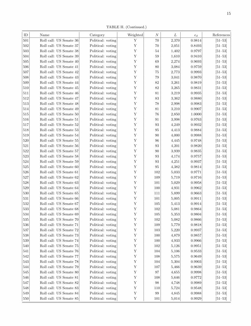
15
TABLE II. (Continued.)
ID Name Category Weighted N L ed References
501 Roll call: US Senate 36 Political: voting Y 70 2,370 0.9814 [51–53]
502 Roll call: US Senate 37 Political: voting Y 70 2,051 0.8493 [51–53]
503 Roll call: US Senate 38 Political: voting Y 54 1,402 0.9797 [51–53]
504 Roll call: US Senate 39 Political: voting Y 59 1,610 0.9410 [51–53]
505 Roll call: US Senate 40 Political: voting Y 69 2,274 0.9693 [51–53]
506 Roll call: US Senate 41 Political: voting Y 80 3,084 0.9759 [51–53]
507 Roll call: US Senate 42 Political: voting Y 75 2,773 0.9993 [51–53]
508 Roll call: US Senate 43 Political: voting Y 79 3,041 0.9870 [51–53]
509 Roll call: US Senate 44 Political: voting Y 82 3,261 0.9819 [51–53]
510 Roll call: US Senate 45 Political: voting Y 82 3,265 0.9831 [51–53]
511 Roll call: US Senate 46 Political: voting Y 81 3,219 0.9935 [51–53]
512 Roll call: US Senate 47 Political: voting Y 83 3,362 0.9880 [51–53]
513 Roll call: US Senate 48 Political: voting Y 78 2,998 0.9983 [51–53]
514 Roll call: US Senate 49 Political: voting Y 81 3,210 0.9907 [51–53]
515 Roll call: US Senate 50 Political: voting Y 76 2,850 1.0000 [51–53]
516 Roll call: US Senate 51 Political: voting Y 91 3,998 0.9763 [51–53]
517 Roll call: US Senate 52 Political: voting Y 93 4,249 0.9932 [51–53]
518 Roll call: US Senate 53 Political: voting Y 95 4,413 0.9884 [51–53]
519 Roll call: US Senate 54 Political: voting Y 90 4,000 0.9988 [51–53]
520 Roll call: US Senate 55 Political: voting Y 96 4,445 0.9748 [51–53]
521 Roll call: US Senate 56 Political: voting Y 93 4,201 0.9820 [51–53]
522 Roll call: US Senate 57 Political: voting Y 90 3,939 0.9835 [51–53]
523 Roll call: US Senate 58 Political: voting Y 93 4,174 0.9757 [51–53]
524 Roll call: US Senate 59 Political: voting Y 93 4,251 0.9937 [51–53]
525 Roll call: US Senate 60 Political: voting Y 95 4,382 0.9814 [51–53]
526 Roll call: US Senate 61 Political: voting Y 102 5,033 0.9771 [51–53]
527 Roll call: US Senate 62 Political: voting Y 109 5,719 0.9716 [51–53]
528 Roll call: US Senate 63 Political: voting Y 101 5,029 0.9958 [51–53]
529 Roll call: US Senate 64 Political: voting Y 100 4,931 0.9962 [51–53]
530 Roll call: US Senate 65 Political: voting Y 111 5,899 0.9663 [51–53]
531 Roll call: US Senate 66 Political: voting Y 101 5,005 0.9911 [51–53]
532 Roll call: US Senate 67 Political: voting Y 105 5,413 0.9914 [51–53]
533 Roll call: US Senate 68 Political: voting Y 102 5,081 0.9864 [51–53]
534 Roll call: US Senate 69 Political: voting Y 105 5,353 0.9804 [51–53]
535 Roll call: US Senate 70 Political: voting Y 102 5,082 0.9866 [51–53]
536 Roll call: US Senate 71 Political: voting Y 109 5,779 0.9818 [51–53]
537 Roll call: US Senate 72 Political: voting Y 103 5,220 0.9937 [51–53]
538 Roll call: US Senate 73 Political: voting Y 100 4,879 0.9857 [51–53]
539 Roll call: US Senate 74 Political: voting Y 100 4,933 0.9966 [51–53]
540 Roll call: US Senate 75 Political: voting Y 102 5,126 0.9951 [51–53]
541 Roll call: US Senate 76 Political: voting Y 104 5,106 0.9533 [51–53]
542 Roll call: US Senate 77 Political: voting Y 108 5,575 0.9649 [51–53]
543 Roll call: US Senate 78 Political: voting Y 104 5,304 0.9903 [51–53]
544 Roll call: US Senate 79 Political: voting Y 107 5,466 0.9639 [51–53]
545 Roll call: US Senate 80 Political: voting Y 97 4,655 0.9998 [51–53]
546 Roll call: US Senate 81 Political: voting Y 108 5,646 0.9772 [51–53]
547 Roll call: US Senate 82 Political: voting Y 98 4,748 0.9989 [51–53]
548 Roll call: US Senate 83 Political: voting Y 110 5,724 0.9548 [51–53]
549 Roll call: US Senate 84 Political: voting Y 99 4,845 0.9988 [51–53]
550 Roll call: US Senate 85 Political: voting Y 101 5,014 0.9929 [51–53]

16
TABLE II. (Continued.)
ID Name Category Weighted N L ed References
551 Roll call: US Senate 86 Political: voting Y 103 5,246 0.9987 [51–53]
552 Roll call: US Senate 87 Political: voting Y 105 5,444 0.9971 [51–53]
553 Roll call: US Senate 88 Political: voting Y 103 5,249 0.9992 [51–53]
554 Roll call: US Senate 89 Political: voting Y 103 5,247 0.9989 [51–53]
555 Roll call: US Senate 90 Political: voting Y 101 5,048 0.9996 [51–53]
556 Roll call: US Senate 91 Political: voting Y 102 5,148 0.9994 [51–53]
557 Roll call: US Senate 92 Political: voting Y 102 5,147 0.9992 [51–53]
558 Roll call: US Senate 93 Political: voting Y 103 5,246 0.9987 [51–53]
559 Roll call: US Senate 94 Political: voting Y 101 5,049 0.9998 [51–53]
560 Roll call: US Senate 95 Political: voting Y 104 5,345 0.9979 [51–53]
561 Roll call: US Senate 96 Political: voting Y 101 5,049 0.9998 [51–53]
562 Roll call: US Senate 97 Political: voting Y 101 5,049 0.9998 [51–53]
563 Roll call: US Senate 98 Political: voting Y 101 5,049 0.9998 [51–53]
564 Roll call: US Senate 99 Political: voting Y 101 5,049 0.9998 [51–53]
565 Roll call: US Senate 100 Political: voting Y 101 5,049 0.9998 [51–53]
566 Roll call: US Senate 101 Political: voting Y 100 4,950 1.0000 [51–53]
567 Roll call: US Senate 102 Political: voting Y 102 5,148 0.9994 [51–53]
568 Roll call: US Senate 103 Political: voting Y 102 5,080 0.9862 [51–53]
569 Roll call: US Senate 104 Political: voting Y 103 5,247 0.9989 [51–53]
570 Roll call: US Senate 105 Political: voting Y 100 4,950 1.0000 [51–53]
571 Roll call: US Senate 106 Political: voting Y 102 5,148 0.9994 [51–53]
571 Roll call: US Senate 107 Political: voting Y 102 5,148 0.9994 [51–53]
573 Roll call: US Senate 108 Political: voting Y 100 4,950 1.0000 [51–53]
574 Roll call: US Senate 109 Political: voting Y 101 5,049 0.9998 [51–53]
575 Roll call: US Senate 110 Political: voting Y 102 5,147 0.9992 [51–53]
576 UK House of Commons voting: 1992-1997 Political: voting Y 668 220,761 0.9909 [54]
577 UK House of Commons voting: 1997-2001 Political: voting Y 671 223,092 0.9925 [54]
578 UK House of Commons voting: 2001-2005 Political: voting Y 657 215,246 0.9988 [54]
579 UN resolutions 1 Political: voting Y 54 1,431 1.0000 [55]
580 UN resolutions 2 Political: voting Y 57 1,594 0.9987 [55]
581 UN resolutions 3 Political: voting Y 59 1,711 1.0000 [55]
582 UN resolutions 4 Political: voting Y 59 1,711 1.0000 [55]
583 UN resolutions 5 Political: voting Y 60 1,770 1.0000 [55]
584 UN resolutions 6 Political: voting Y 60 1,768 0.9989 [55]
585 UN resolutions 7 Political: voting Y 60 1,770 1.0000 [55]
586 UN resolutions 8 Political: voting Y 60 1,770 1.0000 [55]
587 UN resolutions 9 Political: voting Y 60 1,770 1.0000 [55]
588 UN resolutions 10 Political: voting Y 65 2,037 0.9793 [55]
589 UN resolutions 11 Political: voting Y 81 3,239 0.9997 [55]
590 UN resolutions 12 Political: voting Y 82 3,317 0.9988 [55]
591 UN resolutions 13 Political: voting Y 82 3,294 0.9919 [55]
592 UN resolutions 14 Political: voting Y 82 3,321 1.0000 [55]
593 UN resolutions 15 Political: voting Y 99 4,851 1.0000 [55]
594 UN resolutions 16 Political: voting Y 104 5,356 1.0000 [55]
595 UN resolutions 17 Political: voting Y 110 5,995 1.0000 [55]
596 UN resolutions 18 Political: voting Y 113 6,246 0.9870 [55]
597 UN resolutions 20 Political: voting Y 117 6,672 0.9832 [55]
598 UN resolutions 21 Political: voting Y 122 7,333 0.9935 [55]
599 UN resolutions 22 Political: voting Y 124 7,616 0.9987 [55]
600 UN resolutions 23 Political: voting Y 126 7,855 0.9975 [55]
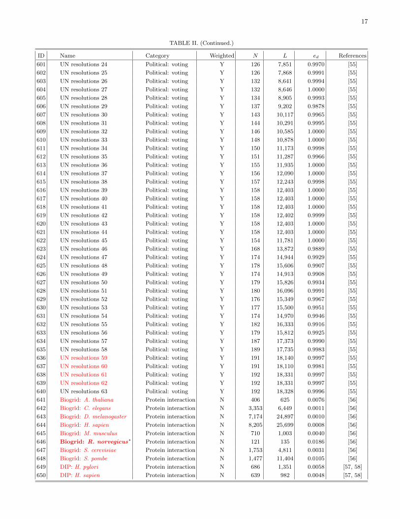
17
TABLE II. (Continued.)
ID Name Category Weighted N L ed References
601 UN resolutions 24 Political: voting Y 126 7,851 0.9970 [55]
602 UN resolutions 25 Political: voting Y 126 7,868 0.9991 [55]
603 UN resolutions 26 Political: voting Y 132 8,641 0.9994 [55]
604 UN resolutions 27 Political: voting Y 132 8,646 1.0000 [55]
605 UN resolutions 28 Political: voting Y 134 8,905 0.9993 [55]
606 UN resolutions 29 Political: voting Y 137 9,202 0.9878 [55]
607 UN resolutions 30 Political: voting Y 143 10,117 0.9965 [55]
608 UN resolutions 31 Political: voting Y 144 10,291 0.9995 [55]
609 UN resolutions 32 Political: voting Y 146 10,585 1.0000 [55]
610 UN resolutions 33 Political: voting Y 148 10,878 1.0000 [55]
611 UN resolutions 34 Political: voting Y 150 11,173 0.9998 [55]
612 UN resolutions 35 Political: voting Y 151 11,287 0.9966 [55]
613 UN resolutions 36 Political: voting Y 155 11,935 1.0000 [55]
614 UN resolutions 37 Political: voting Y 156 12,090 1.0000 [55]
615 UN resolutions 38 Political: voting Y 157 12,243 0.9998 [55]
616 UN resolutions 39 Political: voting Y 158 12,403 1.0000 [55]
617 UN resolutions 40 Political: voting Y 158 12,403 1.0000 [55]
618 UN resolutions 41 Political: voting Y 158 12,403 1.0000 [55]
619 UN resolutions 42 Political: voting Y 158 12,402 0.9999 [55]
620 UN resolutions 43 Political: voting Y 158 12,403 1.0000 [55]
621 UN resolutions 44 Political: voting Y 158 12,403 1.0000 [55]
622 UN resolutions 45 Political: voting Y 154 11,781 1.0000 [55]
623 UN resolutions 46 Political: voting Y 168 13,872 0.9889 [55]
624 UN resolutions 47 Political: voting Y 174 14,944 0.9929 [55]
625 UN resolutions 48 Political: voting Y 178 15,606 0.9907 [55]
626 UN resolutions 49 Political: voting Y 174 14,913 0.9908 [55]
627 UN resolutions 50 Political: voting Y 179 15,826 0.9934 [55]
628 UN resolutions 51 Political: voting Y 180 16,096 0.9991 [55]
629 UN resolutions 52 Political: voting Y 176 15,349 0.9967 [55]
630 UN resolutions 53 Political: voting Y 177 15,500 0.9951 [55]
631 UN resolutions 54 Political: voting Y 174 14,970 0.9946 [55]
632 UN resolutions 55 Political: voting Y 182 16,333 0.9916 [55]
633 UN resolutions 56 Political: voting Y 179 15,812 0.9925 [55]
634 UN resolutions 57 Political: voting Y 187 17,373 0.9990 [55]
635 UN resolutions 58 Political: voting Y 189 17,735 0.9983 [55]
636 UN resolutions 59 Political: voting Y 191 18,140 0.9997 [55]
637 UN resolutions 60 Political: voting Y 191 18,110 0.9981 [55]
638 UN resolutions 61 Political: voting Y 192 18,331 0.9997 [55]
639 UN resolutions 62 Political: voting Y 192 18,331 0.9997 [55]
640 UN resolutions 63 Political: voting Y 192 18,328 0.9996 [55]
641 Biogrid: A. thaliana Protein interaction N 406 625 0.0076 [56]
642 Biogrid: C. elegans Protein interaction N 3,353 6,449 0.0011 [56]
643 Biogrid: D. melanogaster Protein interaction N 7,174 24,897 0.0010 [56]
644 Biogrid: H. sapien Protein interaction N 8,205 25,699 0.0008 [56]
645 Biogrid: M. musculus Protein interaction N 710 1,003 0.0040 [56]
646 Biogrid: R. norvegicus∗ Protein interaction N 121 135 0.0186 [56]
647 Biogrid: S. cerevisiae Protein interaction N 1,753 4,811 0.0031 [56]
648 Biogrid: S. pombe Protein interaction N 1,477 11,404 0.0105 [56]
649 DIP: H. pylori Protein interaction N 686 1,351 0.0058 [57, 58]
650 DIP: H. sapien Protein interaction N 639 982 0.0048 [57, 58]

18
TABLE II. (Continued.)
ID Name Category Weighted N L ed References
651 DIP: M. musculus Protein interaction N 50 55 0.0449 [57, 58]
651 DIP: C. elegans Protein interaction N 2,386 3,825 0.0013 [57, 58]
653 Human: Ccsb Protein interaction N 1,307 2,483 0.0029 [59]
654 Human: Ophid Protein interaction N 5,464 23,238 0.0016 [60, 61]
655 STRING: C. elegans Protein interaction N 1,762 95,227 0.0614 [62]
656 STRING: S. cerevisiae Protein interaction N 534 57,672 0.4053 [62]
657 Yeast: Oxford Statistics Protein interaction N 2,224 6,609 0.0027 [63]
658 Yeast: DIP Protein interaction N 4,906 17,218 0.0014 [57, 58, 63]
659 Yeast: DIPC Protein interaction N 2,587 6,094 0.0018 [57, 58, 63]
660 Yeast: FHC Protein interaction N 2,233 5,750 0.0023 [63, 64]
661 Yeast: FYI Protein interaction N 778 1,798 0.0059 [63, 65]
662 Yeast: PCA Protein interaction N 889 2,407 0.0061 [63, 66]
663 Corporate directors in Scotland (1904–1905)∗ Social Y 131 676 0.0794 [16, 67]
664 Corporate ownership (EVA) Social N 4,475 4,652 0.0005 [68]
665 Dolphins∗ Social N 62 159 0.0841 [69]
666 Family planning in Korea Social N 33 68 0.1288 [70]
667 Unionization in a high-tech firm∗ Social N 33 91 0.1723 [71]
668 Communication within a sawmill on strike∗ Social N 36 62 0.0984 [72]
669 Leadership course Social N 32 80 0.1613 [33]
670 Les Miserables∗ Social Y 77 254 0.0868 [32]
671 Marvel comics Social Y 6,449 168,211 0.0081 [73]
672 Mexican political elite Social N 35 117 0.1966 [74]
673 Pretty-good-privacy (PGP) algorithm users Social N 10,680 24,316 0.0004 [75]
674 Prisoners Social N 67 142 0.0642 [33]
675 Bernard and Killworth fraternity: observed Social Y 58 967 0.5850 [76–78]
676 Bernard and Killworth fraternity: recalled Social Y 58 1,653 1.0000 [76–78]
677 Bernard and Killworth HAM radio: observed Social Y 41 153 0.1866 [79–81]
678 Bernard and Killworth HAM radio: recalled Social Y 44 442 0.4672 [79–81]
679 Bernard and Killworth office: observed Social Y 40 238 0.3051 [79–81]
680 Bernard and Killworth office: recalled Social Y 40 779 0.9987 [79–81]
681 Bernard and Killworth technical: observed Social Y 34 175 0.3119 [79–81]
681 Bernard and Killworth technical: recalled Social Y 34 561 1.0000 [79–81]
683 Kapferer tailor shop: instrumental (t1) Social N 35 76 0.1277 [82]
684 Kapferer tailor shop: instrumental (t2) Social N 34 93 0.1658 [82]
685 Kapferer tailor shop: associational (t1) Social N 39 158 0.2132 [82]
686 Kapferer tailor shop: associational (t2) Social N 39 223 0.3009 [82]
687 University Rovira i Virgili (Tarragona) e-mail Social N 1,133 5,451 0.0085 [83]
688 Zachary karate club∗ Social N 34 78 0.1390 [84]
689 BA: (100,1)∗ Synthetic N 100 99 0.0200 [3]
690 BA: (100,2)∗ Synthetic N 100 197 0.0398 [3]
691 BA: (1000,1) Synthetic N 1,000 999 0.0020 [3]
692 BA: (1000,2) Synthetic N 1,000 1,997 0.0040 [3]
693 BA: (500,1) Synthetic N 500 499 0.0040 [3]
694 BA: (500,2) Synthetic N 500 997 0.0080 [3]
695 ER: (100,0.25)∗ Synthetic N 100 1,264 0.2554 [1]
696 ER: (100,0.5) Synthetic N 100 2,436 0.4921 [1]
697 ER: (100,0.75) Synthetic N 100 3,697 0.7469 [1]
698 ER: (500,0.25) Synthetic N 500 31,148 0.2497 [1]
699 ER: (500,0.5) Synthetic N 500 62,301 0.4994 [1]
700 ER: (500,75) Synthetic N 500 93,780 0.7517 [1]
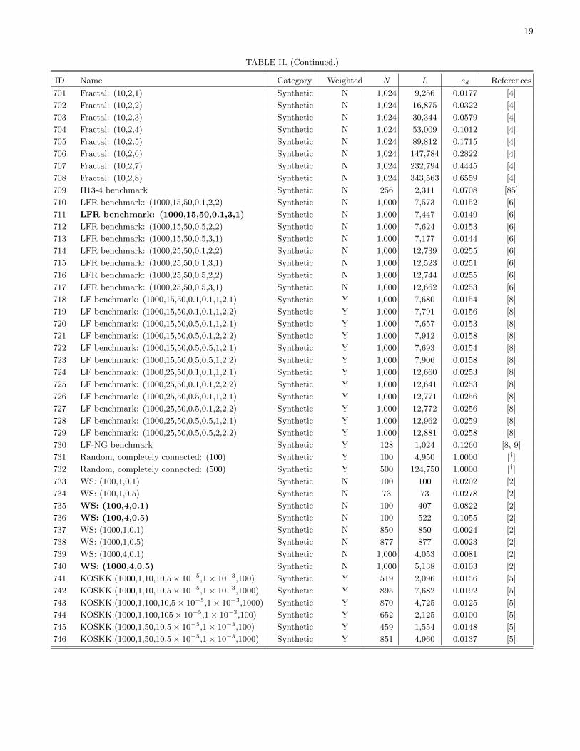
19
TABLE II. (Continued.)
ID Name Category Weighted N L ed References
701 Fractal: (10,2,1) Synthetic N 1,024 9,256 0.0177 [4]
702 Fractal: (10,2,2) Synthetic N 1,024 16,875 0.0322 [4]
703 Fractal: (10,2,3) Synthetic N 1,024 30,344 0.0579 [4]
704 Fractal: (10,2,4) Synthetic N 1,024 53,009 0.1012 [4]
705 Fractal: (10,2,5) Synthetic N 1,024 89,812 0.1715 [4]
706 Fractal: (10,2,6) Synthetic N 1,024 147,784 0.2822 [4]
707 Fractal: (10,2,7) Synthetic N 1,024 232,794 0.4445 [4]
708 Fractal: (10,2,8) Synthetic N 1,024 343,563 0.6559 [4]
709 H13-4 benchmark Synthetic N 256 2,311 0.0708 [85]
710 LFR benchmark: (1000,15,50,0.1,2,2) Synthetic N 1,000 7,573 0.0152 [6]
711 LFR benchmark: (1000,15,50,0.1,3,1) Synthetic N 1,000 7,447 0.0149 [6]
712 LFR benchmark: (1000,15,50,0.5,2,2) Synthetic N 1,000 7,624 0.0153 [6]
713 LFR benchmark: (1000,15,50,0.5,3,1) Synthetic N 1,000 7,177 0.0144 [6]
714 LFR benchmark: (1000,25,50,0.1,2,2) Synthetic N 1,000 12,739 0.0255 [6]
715 LFR benchmark: (1000,25,50,0.1,3,1) Synthetic N 1,000 12,523 0.0251 [6]
716 LFR benchmark: (1000,25,50,0.5,2,2) Synthetic N 1,000 12,744 0.0255 [6]
717 LFR benchmark: (1000,25,50,0.5,3,1) Synthetic N 1,000 12,662 0.0253 [6]
718 LF benchmark: (1000,15,50,0.1,0.1,1,2,1) Synthetic Y 1,000 7,680 0.0154 [8]
719 LF benchmark: (1000,15,50,0.1,0.1,1,2,2) Synthetic Y 1,000 7,791 0.0156 [8]
720 LF benchmark: (1000,15,50,0.5,0.1,1,2,1) Synthetic Y 1,000 7,657 0.0153 [8]
721 LF benchmark: (1000,15,50,0.5,0.1,2,2,2) Synthetic Y 1,000 7,912 0.0158 [8]
722 LF benchmark: (1000,15,50,0.5,0.5,1,2,1) Synthetic Y 1,000 7,693 0.0154 [8]
723 LF benchmark: (1000,15,50,0.5,0.5,1,2,2) Synthetic Y 1,000 7,906 0.0158 [8]
724 LF benchmark: (1000,25,50,0.1,0.1,1,2,1) Synthetic Y 1,000 12,660 0.0253 [8]
725 LF benchmark: (1000,25,50,0.1,0.1,2,2,2) Synthetic Y 1,000 12,641 0.0253 [8]
726 LF benchmark: (1000,25,50,0.5,0.1,1,2,1) Synthetic Y 1,000 12,771 0.0256 [8]
727 LF benchmark: (1000,25,50,0.5,0.1,2,2,2) Synthetic Y 1,000 12,772 0.0256 [8]
728 LF benchmark: (1000,25,50,0.5,0.5,1,2,1) Synthetic Y 1,000 12,962 0.0259 [8]
729 LF benchmark: (1000,25,50,0.5,0.5,2,2,2) Synthetic Y 1,000 12,881 0.0258 [8]
730 LF-NG benchmark Synthetic Y 128 1,024 0.1260 [8, 9]
731 Random, completely connected: (100) Synthetic Y 100 4,950 1.0000 [†]
732 Random, completely connected: (500) Synthetic Y 500 124,750 1.0000 [†]
733 WS: (100,1,0.1) Synthetic N 100 100 0.0202 [2]
734 WS: (100,1,0.5) Synthetic N 73 73 0.0278 [2]
735 WS: (100,4,0.1) Synthetic N 100 407 0.0822 [2]
736 WS: (100,4,0.5) Synthetic N 100 522 0.1055 [2]
737 WS: (1000,1,0.1) Synthetic N 850 850 0.0024 [2]
738 WS: (1000,1,0.5) Synthetic N 877 877 0.0023 [2]
739 WS: (1000,4,0.1) Synthetic N 1,000 4,053 0.0081 [2]
740 WS: (1000,4,0.5) Synthetic N 1,000 5,138 0.0103 [2]
741 KOSKK:(1000,1,10,10,5× 10−5,1× 10−3,100) Synthetic Y 519 2,096 0.0156 [5]
742 KOSKK:(1000,1,10,10,5× 10−5,1× 10−3,1000) Synthetic Y 895 7,682 0.0192 [5]
743 KOSKK:(1000,1,100,10,5× 10−5,1× 10−3,1000) Synthetic Y 870 4,725 0.0125 [5]
744 KOSKK:(1000,1,100,105× 10−5,1× 10−3,100) Synthetic Y 652 2,125 0.0100 [5]
745 KOSKK:(1000,1,50,10,5× 10−5,1× 10−3,100) Synthetic Y 459 1,554 0.0148 [5]
746 KOSKK:(1000,1,50,10,5× 10−5,1× 10−3,1000) Synthetic Y 851 4,960 0.0137 [5]

20
[1] P. Erdos and A. Renyi, Publicationes Mathematicae 6, 290 (1959).[2] D. J. Watts and S. H. Strogatz, Nature 393, 440 (1998).[3] A.-L. Barabasi and R. Albert, Science 286, 509 (1999).[4] O. Sporns, BioSystems 85, 55 (2006).[5] J. M. Kumpula, J.-P. Onnela, J. Saramaki, K. Kaski, and J. Kertesz, Physical Review Letters 99, 228701 (2007).[6] A. Lancichinetti, S. Fortunato, and F. Radicchi, Physical Review E 78, 046110 (2008).[7] M. Molloy and B. Reed, Random Structures and Algorithms 6, 161 (1995).[8] A. Lancichinetti and S. Fortunato, Physical Review E 80, 016118 (2009).[9] M. E. J. Newman and M. Girvan, Physical Review E 69, 026113 (2004).
[10] P. Hagmann, L. Cammoun, X. Gigandet, R. Meuli, C. J. Honey, V. J. Wedeen, and O. Sporns, PLoS Biology 6, e159(2008).
[11] J. W. Scannell, G. A. P. C. Burns, C. C. Hilgetag, M. A. O’Neil, and M. P. Young, Cerebral Cortex 9, 277 (1999).[12] D. J. Felleman and D. C. V. Essen, Cerebral Cortex 1, 1 (1991).[13] M. P. Young, Proceedings of the Royal Society B 252, 13 (1993).[14] M. E. J. Newman, Proceedings of the National Academy of Sciences of the U.S.A. 98, 404 (2001).[15] N. H. F. Beebe, (2002). The author collaboration network in computational geometry was produced from the BibTeX
bibliography available at http://www.math.utah.edu/~beebe/bibliographies.html. The network data is available athttp://vlado.fmf.uni-lj.si/pub/networks/data/collab/geom.htm.
[16] W. de Nooy, A. Mrvar, and V. Batagelj, Exploratory Social Network Analysis with Pajek (Cambridge University Press,Cambridge, UK, 2004).
[17] V. Batagelj and A. Mrvar, (2006). The data is available at http://vlado.fmf.uni-lj.si/pub/networks/data/default.htm.
[18] M. E. J. Newman, Physical Review E 74, 036104 (2006).[19] R. R. Faulkner, Music on Demand. Composers and Careers in the Hollywood Film Industry (Transaction Books, New
Brunswick, NJ, USA, 1983).[20] P. Gleiser and L. Danon, Advances in Complex Systems 6, 565 (2003).[21] A. L. Traud, E. D. Kelsic, P. J. Mucha, and M. A. Porter, SIAM Review 53, 526 (2011).[22] A. L. Traud, P. J. Mucha, and M. A. Porter, Physica A 391, 4165 (2012).[23] J.-P. Onnela, A. Chakraborti, K. Kaski, J. Kertesz, and A. Kanto, Physical Review E 68, 056110 (2003).[24] D. J. Fenn, (2008). Data downloaded on 19 December 2008 from http://uk.finance.yahoo.com/.[25] A. Tero, S. Takagi, T. Saigusa, K. Ito, D. P. Bebber, M. D. Fricker, K. Yumiki, R. Kobayashi, and T. Nakagaki, Science
327, 439 (2010).[26] M. D. Fricker, L. Boddy, and D. P. Bebber, Topologica 1, 4 (2008).[27] L. L. M. Heaton, E. Lopez, P. K. Maini, M. D. Fricker, and N. S. Jones, Proceedings of the Royal Society B 277, 3265
(2010).[28] D. P. Bebber, J. Hynes, P. R. Darrah, L. Boddy, and M. D. Fricker, Proceedings of the Royal Society B 274, 2307 (2007).[29] V. Batagelj, A. Mrvar, and M. Zaversnik, in Proceedings of the 5th International Multi-Conference Information Society –
Language Technologies, edited by T.Erjavec and J. Gros (2002) pp. 143–148.[30] J. M. Reitz, (2000), ODLIS is maintained by Joan Reitz and was converted into the network used here by A. Mrvar and
V. Batagelj. The data is available at http://vlado.fmf.uni-lj.si/pub/networks/data/dic/odlis/Odlis.htm.[31] J. C. Johnson and L. Krempel, Journal of Social Structures 5 (2004).[32] D. E. Knuth, The Stanford GraphBase: A Platform for Combinatorial Computing (Addison-Wesley, Reading, MA, USA,
1993).[33] R. Milo, S. Itzkovitz, N. Kashtan, R. Levittand, S. Shen-Orr, I. Ayzenshtat, M. Sheffer, and U. Alon, Science 303, 1538
(2004).[34] H. Jeong, B. Tombor, R. Albert, Z. N. Oltvai, and A.-L. Barabasi, Nature 407, 651 (2000).[35] V. Krebs, (2004). The network was compiled by Valdis Krebs. The data is available at http://www.orgnet.com/.[36] V. Batagelj, (2003). The data is available at http://vlado.fmf.uni-lj.si/pub/networks/data/2mode/journals.htm.[37] S. Mangan and U. Alon, Proceedings of the National Academy of Sciences of the U.S.A. 100, 11980 (2003).[38] R. Milo, S. Shen-Orr, S. Itzkovitz, N. Kashtan, D. Chklovskii, and U. Alon, Science 298, 824 (2002).[39] T. Callaghan, P. J. Mucha, and M. A. Porter, American Mathematical Monthly 114, 761 (2007).[40] M. E. J. Newman, (2006). The network was compiled by Mark Newman. The data is available at http://www-personal.
umich.edu/~mejn/netdata/.[41] E. Garfield, I. H. Sher, and R. J. Torpie, The Use of Citation Data in Writing the History of Science (The Institute for
Scientific Information, Philadelphia, PA, USA, 1964).[42] S. Gopal, Societies and Cities in the Age of Instant Access, (Springer Verlag, Berlin, Germany, 2007).[43] L. A. Adamic and N. Glance, in LinkKDD ’05: Proceedings of the 3rd international workshop on Link discovery (2005)
pp. 36–43.[44] D. F. Gleich, (2001). The data is available at http://www.cise.ufl.edu/research/sparse/matrices/Gleich/
wb-cs-stanford.html.[45] C. A. Hidalgo, B. Klinger, A. L. Barabasi, and R. Hausmann, Science 317, 482 (2007).
21
[46] D. A. Smith and D. R. White, Social Forces 70, 857 (1992).[47] J. H. Fowler, Social Networks 28, 454 (2006).[48] J. H. Fowler, Political Analysis 14, 456 (2006).[49] M. A. Porter, P. J. Mucha, M. E. J. Newman, and C. M. Warmbrand, Proceedings of the National Academy of Sciences
of the U.S.A. 102, 7057 (2005).[50] M. A. Porter, P. J. Mucha, M. E. J. Newman, and A. J. Friend, Physica A 386, 414 (2007).[51] A. S. Waugh, L. Pei, J. H. Fowler, P. J.Mucha, and M. A. Porter, arXiv:0907.3509 (2012).[52] K. T. Poole and H. Rosenthal, Congress: A Political-Economic History of Roll Call Voting (Oxford University Press,
Oxford, UK, 1997).[53] N. M. McCarty, K. T. Poole, and H. Rosenthal, Polarized America: The Dance of Ideology and Unequal Riches (MIT
Press, Cambridge, MA, USA, 2007).[54] D. Firth and A. Spirling, working paper (2003), available at http://www2.warwick.ac.uk/fac/sci/statistics/staff/
academic/firth/software/tapir/firth-spirling.pdf.[55] E. Voeten, International Organization 54, 185 (2000).[56] C. Stark, B. J. Breitkreutz, T. Reguly, L. Boucher, A. Breitkreutz, and M. Tyers, Nucleic Acids Research 34, D535 (2006).[57] L. Salwinski, C. S. Miller, A. J. Smith, F. K. Pettit, J. U. Bowie, and D. Eisenberg, Nucleic Acids Research 32, D449
(2004).[58] I. Xenarios, L. Salwinski, X. J. Duan, P. Higney, S. M. Kim, and D. Eisenberg, Nucleic acids research 30, 303 (2002).[59] J. F. Rual, K. Venkatesan, T. Hao, T. Hirozane-Kishikawa, A. Dricot, N. Li, G. F. Berriz, F. D. Gibbons, M. Dreze,
N. Ayivi-Guedehoussou, and et al., Nature 437, 1173 (2005).[60] K. Brown and I. Jurisica, Genome Biology 8, R95 (2007).[61] K. R. Brown and I. Jurisica, Bioinformatics 21, 2076 (2005).[62] L. J. Jensen, M. Kuhn, M. Stark, S. Chaffron, C. Creevey, J. Muller, T. Doerks, P. Julien, A. Roth, M. Simonovic, P. Bork,
and C. von Mering, Nucleic Acids Research 37, D412 (2009).[63] S. Agarwal, C. M. Deane, M. A. Porter, and N. S. Jones, PLoS Computational Biology 6, e1000817 (2010).[64] N. Bertin, N. Simonis, D. Dupuy, M. E. Cusick, J. D. J. Han, H. B. Fraser, F. P. Roth, and M. Vidal, PLoS Biology 5,
e153 (2007).[65] J. D. J. Han, N. Bertin, T. Hao, D. S. Goldberg, G. F. Berriz, L. V. Zhang, D. Dupuy, A. J. Walhout, M. E. Cusick, F. P.
Roth, and M. Vidal, Nature 430, 88 (2004).[66] K. Tarassov, V. Messier, C. R. Landry, S. Radinovic, M. M. S. Molina, I. Shames, Y. Malitskaya, J. Vogel, H. Bussey, and
S. W. Michnick, Science 320, 1465 (2008).[67] J. Scott and M. Hughes, The Anatomy of Scottish Capital: Scottish Companies and Scottish Capital, 1900–1979 (Croom
Helm, London, UK, 1980).[68] K. Norlen, G. Lucas, M. Gebbie, and J. Chuang, in Proceedings of International Telecommunications Society 14th Biennial
Conference (ITS2002) (2002).[69] D. Lusseau, K. Schneider, O. J. Boisseau, P. Haase, E. Slooten, and S. M. Dawson, Behavioral Ecology and Sociobiology
54, 396 (2003).[70] E. M. Rogers and D. L. Kincaid, Communication Networks. Toward a New Paradigm for Research (The Free Press, New
York, NY, USA, 1981).[71] D. Krackhardt, Research in the Sociology of Organizations 16, 183 (1999).[72] J. H. Michael and J. G. Massey, Forest Products Journal 47, 25 (1997).[73] R. Alberich, J. Miro-Julia, and F. Rossello, arXiv:cond-mat/0202174 (2002).[74] J. Gil-Mendieta and S. Schmidt, Social Networks 18, 355 (1996).[75] M. Boguna, R. Pastor-Satorras, A. Dıaz-Guilera, and A. Arenas, Physical Review E 70, 056122 (2004).[76] H. R. Bernard, P. D. Killworth, and L. Sailer, Social Networks 2, 191 (1979–1980).[77] H. R. Bernard, P. D. Killworth, and L. Sailer, Social Science Research 11, 30 (1982).[78] A. K. Romney and S. C. Weller, Social Networks 6, 59 (1984).[79] H. R. Bernard and P. D. Killworth, Human Organization 35, 269 (1976).[80] H. R. Bernard and P. D. Killworth, Human Communication Research 4, 3 (1977).[81] P. D. Killworth and H. R. Bernard, Social Networks 2, 19 (1979-1980).[82] B. Kapferer, Strategy and Transaction in an African Factory (Manchester University Press, Manchester, UK, 1972).[83] R. Guimera, L. Danon, A. Dıaz-Guilera, F. Giralt, and A. Arenas, Physical Review E 68, 065103 (2003).[84] W. W. Zachary, Journal of Anthropological Research 33, 452 (1977).[85] A. Arenas, A. Dıaz-Guilera, and C. J. Perez-Vicente, Physical Review Letters 96, 114102 (2006).