phy222 lab 2 - electric fields
TRANSCRIPT
Page 1
PHY222 Lab 2 - Electric Fields Mapping the Potential Curves and Field Lines of an Electric Dipole
September 7, 2018
Print Your Name
______________________________________
Print Your Partners' Names
______________________________________
______________________________________
You will return this handout to the instructor at the end of the lab period.
Table of Contents 0. Introduction 1
1. Activity #1: Instructor demonstration 4
2. Activity #2: Experimental setup. 4
3. Activity #3: Plotting equipotential points. 6
4. Activity #4: Plotting the equipotential points using LoggerPro. 8
5. Activity #5: Sketch the equipotential lines and electric field lines. 9
6. Activity #6: Simulating equipotential lines and electric field lines. 10
7. When you are done with this lab… 13
0. Introduction
Abstract. A brief introduction to the notion of the electric field, electric field lines, electric potential and
equipotential lines for a given charge distribution. The relation between equipotential lines and electric field lines is
also discussed.
0.1 Electric field and electric field lines: In the previous lab you explored some of the basic
properties of electric charges. The experimental activities conducted in that lab led you to
conclude that:
(a) there are two types of charges in nature – positive and negative charges,
(b) if charges are brought close to each other they exert an electrostatic force on one another.
(c) the direction of the electric force depends upon the nature of the interacting charges –
like charges repel each other while unlike charges attract each other.
A question that immediately pops up is: How does a charge exert a force on another nearby
charge even though the two charges are not in contact with each other?
To answer this question, physicists in the 19th century hypothesized that with every electric
charge one can associate an Electric field that permeates the space around that electric charge.
The force experienced by a charge in the vicinity of another charge was explained in terms of the
interaction between the charge experiencing the force and the electric field associated with the
Instructions
Before lab, read the Introduction, and
answer the Pre-Lab Questions on the
last page of this handout, complete
Activity #6, and answer questions Q3
and Q4. Hand in your pre-lab
answers as you enter the general
physics lab.
Electric Fields
Page 2
other charge. To make the concept of an electric field more precise, the following properties
were attributed to it:
(a) It is a vector quantity. One can associate a magnitude and a direction to the electric field
for any point near a given charge.
(b) The magnitude or strength of the electric field at a given point is the electrostatic force
experienced by a unit positive charge placed at that point.
(c) The direction of the electric field at any given point is the direction in which a positive
test charge would move starting from rest if placed at that point.
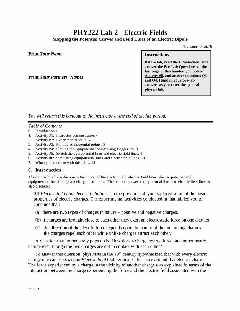
The electric field of a given charge distribution can be visualized by drawing a series of lines
called electric field lines that indicate the direction of the electric field. Examples of electric field
lines for isolated point charges are shown in Figure 1.
-+
Electric field lines
Figure 1 The electric field lines for an isolated positive charge (left) point radially
outward and for an isolated negative charge (right) they point radially inward.
The arrows on the electric field lines indicate the direction of the electric field. Thus in
Figure 1, the positive charge has its field lines pointing outwards while the electric field
lines of a negative charge point inwards.
The number of electric field lines converging to or diverging from a charge is
proportional to the magnitude of the charge. Thus, the greater the amount of charge, the
greater are the number of electric field lines entering or leaving the charge distribution.
The magnitude of the electric field in a given region near a charge is proportional to the
density of the electric field lines. In Figure 1, the electric field is stronger close to the
charges since the electric field lines are closer together while it is weaker as you move
further away since the electric field lines get further apart.
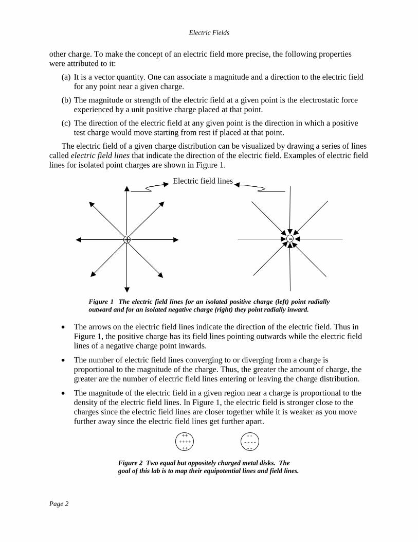
Figure 2 Two equal but oppositely charged metal disks. The
goal of this lab is to map their equipotential lines and field lines.
++
++++
++
- -
- - - -
- -

Electric Fields
Page 3
In the case where one has several charges, the electric field lines around the charge
distribution can be quite involved since the net electric field at a given point is the vector sum of
all the electric fields at that point.
The goal of this lab is to map the electric equipotential lines and the electric field lines
surrounding two metal disks carrying equal and opposite charge (Figure 2).
0.2 Electric potential and equipotential lines
The method we follow to map the electric field lines surrounding a charge distribution
involves the notion of the electric potential. Simply stated, the electric potential at a point near a
charge distribution is the electric energy per unit charge that another charged particle would have
when located at that point. The unit of the electric potential is the Joules/Coulomb = Volt (V).
The probe that you will use in this lab, called a Digital Multimeter, directly measures the
electric potential difference between two points near a charge distribution. If two points are at
the same electric potential then the electric potential difference between the two points is zero.
The two points are referred to as equipotential points and the locus (or set) of all points which
are at the same potential define an equipotential line. One of the tasks in this lab is to trace out
several equipotential lines surrounding the metal disks shown in Figure 2.
0.3 Given the equipotential lines, how do you find the electric field lines?
The electric field lines surrounding a given charge distribution are always perpendicular to
the equipotential lines. Figure 3 shows the equipotential lines and the associated electric field
lines for isolated metal disks carrying a net positive and a net negative charge.
Figure 3 Equipotential lines (dashed lines) and the corresponding electric field lines for an isolated
positively charged metal disk (left) and an isolated negatively charged metal disk (right).
Note that in Figure 1 the electric field lines leaving or entering the metal disks are
perpendicular to the boundary of the disk. This is because the boundary of a charged metal disk
is also an equipotential line.
0.4 How to properly align a push-pin
For reliable results in this lab, you need to press push-pins into a
cork board so that the base of the push-pin is flat and tight against the
surface of the cork board. The diagram to the right shows a side view
of a correctly installed push-pin.
++ + ++++ ++ +
- - - - - - - - - -
Equipotential
lines
Electric Fields
Page 4
1. Activity #1: Instructor demonstration
The Lab Instructor demonstrates aligning and mounting the white graph paper and the black
conductive paper on the cork board. Refer to the instructions under paragraph 2.2.
2. Activity #2: Experimental setup.
Abstract In this activity you set up the equipment in preparation for the measurements of Activity #3.
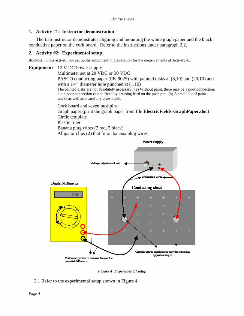
Equipment: 12 V DC Power supply
Multimeter set at 20 VDC or 30 VDC
PASCO conducting paper (PK-9025) with painted disks at (8,10) and (20,10) and
with a 1/4" diameter hole punched at (1,10) The painted disks are not absolutely necessary. (a) Without paint, there may be a poor connection,
but a poor connection can be fixed by pressing hard on the push pin. (b) A small dot of paint
works as well as a carefully drawn disk.
Cork board and seven pushpins
Graph paper (print the graph paper from file ElectricFields-GraphPaper.doc)
Circle template
Plastic ruler
Banana plug wires (2 red, 2 black)
Alligator clips (2) that fit on banana plug wires
Figure 4 Experimental setup
2.1 Refer to the experimental setup shown in Figure 4.

Electric Fields
Page 5
2.1.1 On your table you will find a black conductive paper and a white graph paper.
2.1.2 Two silver-colored conductive disks are painted on the black conductive paper at
locations (8,10) and (20,10) or (6, 10) and (22, 10).
2.1.3 On the white graph paper, the long axis is the horizontal x-axis, and the short axis
is the vertical y-axis.
2.2 Your first task is to mount the black conductive paper and the white graph paper on the
cork board so that their origins and axes are exactly aligned.
2.2.1 Place the white graph paper on the cork board and, using one of the metal
pushpins, punch a hole passing through its origin at (0,0).
2.2.2 Remove the push pin and replace the white graph paper with the black conductive
paper, and punch a hole passing through its center, located at (14, 10).
2.2.3 Now place the black conductive paper and the white graph paper on the cork
board, the black conductive paper on top of the white graph paper and with their grids
facing up. The origins of the two sheets must coincide. This is achieved by poking a
pushpin through the holes you just made and then pressing the pushpin into the cork
board.
2.2.4 You will notice that the black conductive paper has a 1/4" diameter hole located
at the left end of its horizontal axis (the longer axis). You should be able to see the graph
paper though this hole. Orient the two sheets such that the x-axis of the graph paper
exactly coincides with the horizontal axis of the conductive sheet.
2.2.5 Once you have achieved this alignment, fix the two sheets in place by sticking
four pushpins at the four corners of the black conductive paper making sure that they also
pass through the graph paper.
2.2.6 Remove the pushpin at the origin.
2.3 The metal disks on the conductive sheets can be "charged" with the power supply.
2.3.1 Notice that there are two wires originating from your power supply – one from the
positive (red) terminal, the other from the negative (black) terminal.
2.3.2 Push one pushpin into each metal disk. Ensure the pushpin is flat and tight
against the paper under it.
2.3.3 Clip the alligator clip from the black ground power supply terminal to the pushpin
at (8,10) and the alligator clip from the red positive power supply terminal to the pushpin
at (20,10), keeping the wires away from the middle of the conductive black paper.
2.4 Switch the power supply ON. This maintains a constant electric potential difference
between the two metal disks.
2.4.1 This is equivalent to charging the disks with equal but opposite charges.
2.4.2 In particular, the disk connected to the positive terminal (red) of the power supply
is charged positive and the disk connected to the negative terminal (black) is charged
negative.
Electric Fields
Page 6
2.5 The electric potential difference between any two points on the conductive sheet is
measured with the Digital Multimeter (refer Figure 4).
2.5.1 The multimeter should have two probes connected to it. A black probe connected
to the jack marked COM and a red probe to the jack marked V-
2.6 Switch the multimeter ON by turning the selection dial counterclockwise and set it on the
mark labeled 20 V or 30 V. The multimeter is now set to read a maximum potential difference
of 20 V (20 joules per coulomb) or 30 V (30 joules per coulomb).
2.7 Place the metal tip of the black probe from the multimeter in contact with the pushpin on
top of the disk charged negative. Similarly place the red probe on top of the disk charged
positive. Your multimeter will display the electric potential difference between the two
charged disks.
2.8 Adjust the voltage knob on the power supply (see Figure 4) so that the electric potential
difference between the two disks is approximately 12.00 V.
2.9 Notice that if both probes are placed on the same disk your multimeter reading is 0.00V.
This indicates that all points that make up each disk are at the same potential and hence are
equipotential points.
3. Activity #3: Plotting equipotential points. Abstract In this activity you measure the coordinates of the points that will determine the equipotential curves for
an electric dipole.
3.1 Place one of the probes of the multimeter on the conductive paper at the location (6,6),
which will here be referred to as the reference point.
3.2 Lightly press the metal tip of the probe on the reference point so that it leaves a visible
dent on the conductive paper without poking a hole in the paper.
Avoid poking holes in the black paper
until explicitly directed to do so.
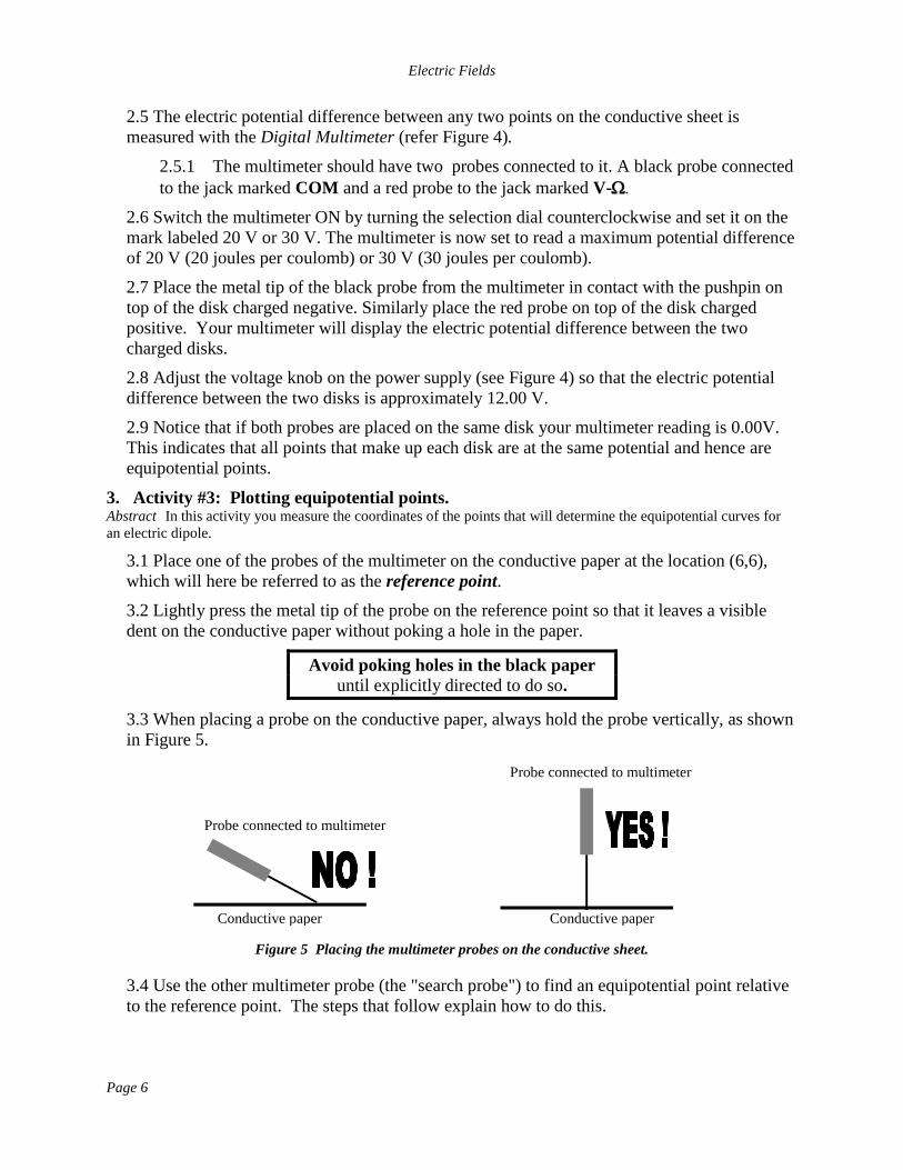
3.3 When placing a probe on the conductive paper, always hold the probe vertically, as shown
in Figure 5.
Figure 5 Placing the multimeter probes on the conductive sheet.
3.4 Use the other multimeter probe (the "search probe") to find an equipotential point relative
to the reference point. The steps that follow explain how to do this.
Conductive paper
Probe connected to multimeter
Conductive paper
Probe connected to multimeter

Electric Fields
Page 7
3.4.1 At an equipotential point on the black conductive paper, your multimeter will read
0.00V, indicating the difference in potential between the location of the search probe and
the location of the reference point is zero volts (i.e., both points have the same voltage).
3.4.2 The best way to find an equipotential point is to start with the search probe close
to the grounded pushpin at (8,10). Then gently drag the search probe directly away from
the pushpin while watching the DMM reading.
3.4.3 When the DMM reading is exactly 0.00 V, you have found an equipotential point
relative to the reference point.
3.4.4 Restrict the search to the area enclosed by the vertical lines at (6,0) and (22,0) and
the horizontal lines (0,4) and (0,16). Refer to Figure 6.
+ + + + + + + + + + +
+ + + + + + + + + + +
+ + + + + + + + + + +
+ + + + + + + + + + +
+ + + + + + + + + + +
+ + + + + + + + + + +
+ + + + + + + + + + +
(6,0) (22,0)
(0,4)
(0,16)
Figure 6 All equipotential points must lie in the
rectangular region enclosed by the four lines.
3.5 For the given reference point, find at least six equipotential points (excluding the
reference point). Restrict attention to the area mentioned in step 3.4.4.
3.5.1 One of the equipotential points must lie on the horizontal axis and another should
lie on or near the vertical line on which the reference point lies. For example, if the
reference point is (6, 6) then one of the equipotential points must be on or near the
vertical line at (6, 0).
3.5.2 There must be equal number of equipotential points above and below the
horizontal axis.
3.5.3 Spread the equipotential points evenly on the search area. Do not pack all the
equipotential points in a small region.
3.5.4 On finding an equipotential point, press the probe firmly on the conductive paper
to leave a visible dent on the paper but without poking a hole through the paper.
3.6 Once you have determined all the equipotential points for the given reference point, circle
the points lightly with a pencil and write the number (1) next to these circles. This will help
you identify the equipotential points later.
3.7 Before you proceed, show your work to your lab instructor and have him or her initial
your lab handout here: Instructor's initials _________
3.8 Change the reference point to (10,4). Repeat steps 3.2-3.6, to obtain a new set of
equipotential points. In step 3.6. replace the number (1) with the number (2) next to the
circles.

Electric Fields
Page 8
3.9 Change the reference point to (14,4). Repeat steps 3.2-3.6, replacing the number (2) with
the number (3) next to the circles.
3.10 Repeat steps 3.2-3.6 for the reference points (18,4) and (22,6) calling the set of
equipotential points (4) and (5) respectively.
3.11 You have now determined points on five different equipotential lines.
Now you can poke holes in the black paper!
3.12 To mark the equipotential points on the graph paper placed below the conductive sheet,
use the spare pushpin to punch holes through all the equipotential points on your conductive
paper.
3.13 Show the conductive paper to your instructor before proceeding.
3.14 Switch the power supply and the multimeter OFF.
3.15 Remove the conductive sheet and the graph paper from the corkboard. On your graph
paper, circle all the equipotential points and label them similar to the conductive sheet.
3.15.1 Notice that on the graph paper, each of the equipotential points corresponds to a
point with a definite (x,y) coordinate.
3.16 Please stick the pushpins on the corkboard to avoid injury.
4. Activity #4: Plotting the equipotential points using LoggerPro.
Abstract In this activity, you have LoggerPro plot the points that define the equipotential curves, so you can print
copies for each member of your group.
Equipment: Computer with LoggerPro
Graph paper and Conductive sheet from Activity #3
Plastic ruler
4.1 Turn ON the computer and open an empty spreadsheet on LoggerPro.
4.2 Create Manual Columns named X and Y.
4.3 Enter the graph paper x and y coordinates of each of the equipotential
points into the spreadsheet.
4.3.1 Use the coordinate system printed on the graph paper, not the
coordinate system on the black conductive paper.
4.3.2 Enter the coordinates in centimeters accurate to one place past
the decimal point. Examples -3.5, 2.0.
4.3.3 Enter all the equipotential points for a given reference point
before entering the set of points for the next reference point. The
figure to the right shows a sample spreadsheet.
4.4 Obtain an X-Y plot of the x and y coordinates of the equipotential
points.
4.4.1 Give a title to the plot. For example, “Plotting the
equipotential points”.
Partner #1:
Partner #2:
Partner #3:
Partner #4:
Reference Equipotential Points
Point x-coordinate y-coordinate
1 … …
… …
… …
… …
… …
… …
… …
2 … …
… …
… …
… …
… …
… …
… …
3 … …
… …
… …
… …
… …
… …
… …
4 … …
… …
… …
… …
… …
… …
… …
5 … …
… …
… …
… …
… …
… …
… …
Sample Spreadsheet
Electric Fields
Page 9
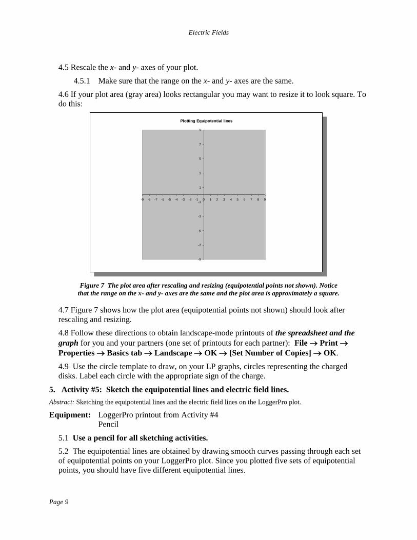
4.5 Rescale the x- and y- axes of your plot.
4.5.1 Make sure that the range on the x- and y- axes are the same.
4.6 If your plot area (gray area) looks rectangular you may want to resize it to look square. To
do this:
Figure 7 The plot area after rescaling and resizing (equipotential points not shown). Notice
that the range on the x- and y- axes are the same and the plot area is approximately a square.
4.7 Figure 7 shows how the plot area (equipotential points not shown) should look after
rescaling and resizing.
4.8 Follow these directions to obtain landscape-mode printouts of the spreadsheet and the
graph for you and your partners (one set of printouts for each partner): File Print
Properties Basics tab Landscape OK [Set Number of Copies] OK.
4.9 Use the circle template to draw, on your LP graphs, circles representing the charged
disks. Label each circle with the appropriate sign of the charge.
5. Activity #5: Sketch the equipotential lines and electric field lines.
Abstract: Sketching the equipotential lines and the electric field lines on the LoggerPro plot.
Equipment: LoggerPro printout from Activity #4
Pencil
5.1 Use a pencil for all sketching activities.
5.2 The equipotential lines are obtained by drawing smooth curves passing through each set
of equipotential points on your LoggerPro plot. Since you plotted five sets of equipotential
points, you should have five different equipotential lines.
Plotting Equipotential lines
-9
-7
-5
-3
-1
1
3
5
7
9
-9 -8 -7 -6 -5 -4 -3 -2 -1 0 1 2 3 4 5 6 7 8 9
Electric Fields
Page 10
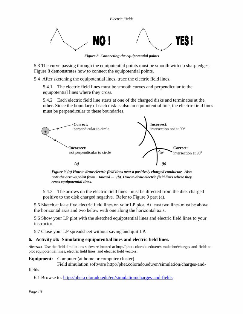
Figure 8 Connecting the equipotential points
5.3 The curve passing through the equipotential points must be smooth with no sharp edges.
Figure 8 demonstrates how to connect the equipotential points.
5.4 After sketching the equipotential lines, trace the electric field lines.
5.4.1 The electric field lines must be smooth curves and perpendicular to the
equipotential lines where they cross.
5.4.2 Each electric field line starts at one of the charged disks and terminates at the
other. Since the boundary of each disk is also an equipotential line, the electric field lines
must be perpendicular to these boundaries.
+
Incorrect:
intersection not at 90º
Correct:
intersection at 90º
(b)
90º
Correct:
perpendicular to circle
Incorrect:
not perpendicular to circle
(a)
Figure 9 (a) How to draw electric field lines near a positively charged conductor. Also
note the arrows point from + toward –. (b) How to draw electric field lines where they
cross equipotential lines.
5.4.3 The arrows on the electric field lines must be directed from the disk charged
positive to the disk charged negative. Refer to Figure 9 part (a).
5.5 Sketch at least five electric field lines on your LP plot. At least two lines must be above
the horizontal axis and two below with one along the horizontal axis.
5.6 Show your LP plot with the sketched equipotential lines and electric field lines to your
instructor.
5.7 Close your LP spreadsheet without saving and quit LP.
6. Activity #6: Simulating equipotential lines and electric field lines.
Abstract Use the field simulations software located at http://phet.colorado.edu/en/simulation/charges-and-fields to
plot equipotential lines, electric field lines, and electric field vectors.
Equipment: Computer (at home or computer cluster)
Field simulation software http://phet.colorado.edu/en/simulation/charges-and-
fields
6.1 Browse to: http://phet.colorado.edu/en/simulation/charges-and-fields
Electric Fields
Page 11
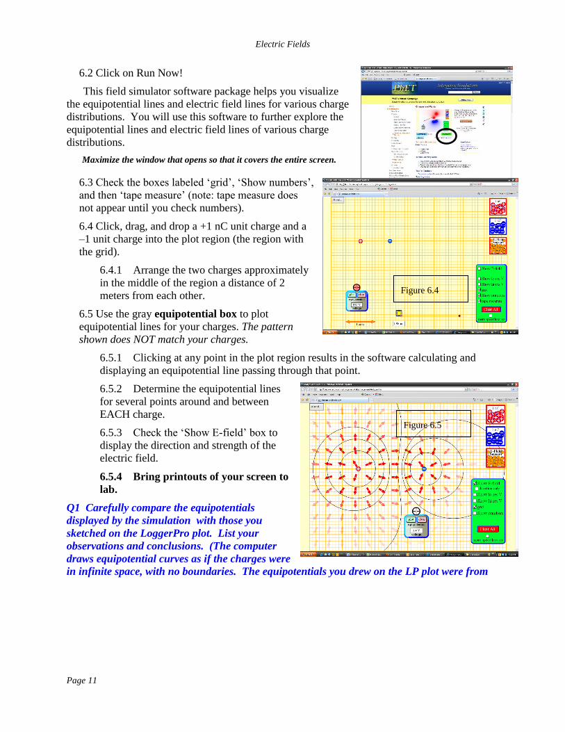
6.2 Click on Run Now!
This field simulator software package helps you visualize
the equipotential lines and electric field lines for various charge
distributions. You will use this software to further explore the
equipotential lines and electric field lines of various charge
distributions.
Maximize the window that opens so that it covers the entire screen.
6.3 Check the boxes labeled ‘grid’, ‘Show numbers’,
and then ‘tape measure’ (note: tape measure does
not appear until you check numbers).
6.4 Click, drag, and drop a +1 nC unit charge and a
–1 unit charge into the plot region (the region with
the grid).
6.4.1 Arrange the two charges approximately
in the middle of the region a distance of 2
meters from each other.
6.5 Use the gray equipotential box to plot
equipotential lines for your charges. The pattern
shown does NOT match your charges.
6.5.1 Clicking at any point in the plot region results in the software calculating and
displaying an equipotential line passing through that point.
6.5.2 Determine the equipotential lines
for several points around and between
EACH charge.
6.5.3 Check the ‘Show E-field’ box to
display the direction and strength of the
electric field.
6.5.4 Bring printouts of your screen to
lab.
Q1 Carefully compare the equipotentials
displayed by the simulation with those you
sketched on the LoggerPro plot. List your
observations and conclusions. (The computer
draws equipotential curves as if the charges were
in infinite space, with no boundaries. The equipotentials you drew on the LP plot were from
Figure 6.4
Figure 6.5

Electric Fields
Page 12
charges confined in a relatively small region – the black paper. Therefore, differences
between the two plots are to be expected.)
Q2 Do the electric field lines plotted here agree with those sketched on your LP plot? List all
your observations and conclusions.
6.6 The following directions will show you how to clear all equipotential lines, electric field
lines and charges from the screen.
6.6.1 To remove all the field lines choose Clear all.
6.7 Place a +4 nC charge close to the middle of the plot region and a –1 nC unit charge two
grids point to its right (1 meter).
6.8 Determine Field vectors for this charge distribution.
6.8.1 Left clicking on an E-field sensor and dragging the mouse to position the sensor
in the plot region displays the direction and magnitude of the electric field in the region
surrounding the charges. If you release the left click button, a vector is displayed
indicating the direction and magnitude of the electric field at the point of release.
6.8.2 To remove displayed Field vectors, drag them back into their storage bin.
Q3 Use the Field vectors tool to find a point on the line joining the two charges where the
electric field vanishes. In the space below sketch the two charges and indicate the point where
Electric Fields
Page 13
you think the electric field vanishes. Include a brief explanation of how you came to this
conclusion.
Hint: Observe the behavior of the Field vectors and the Directional Arrows.
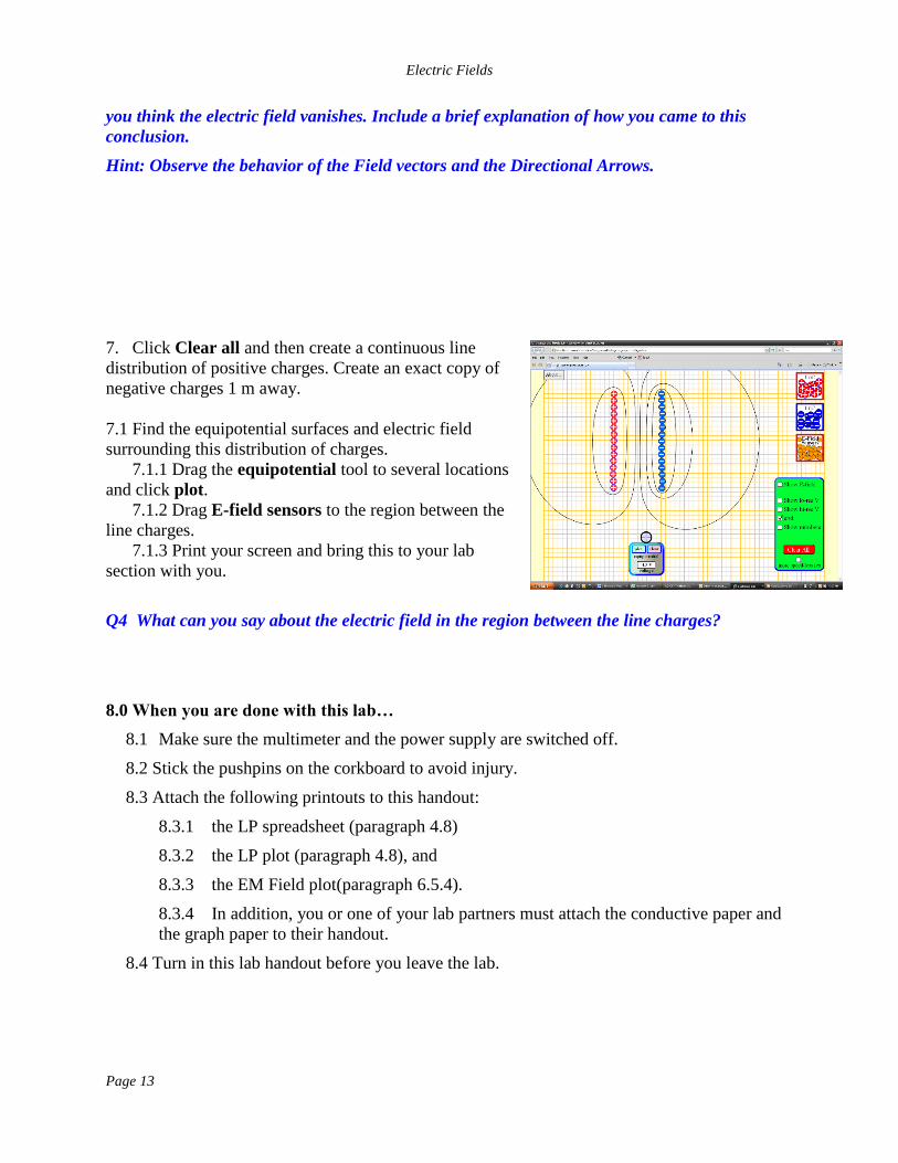
7. Click Clear all and then create a continuous line
distribution of positive charges. Create an exact copy of
negative charges 1 m away.
7.1 Find the equipotential surfaces and electric field
surrounding this distribution of charges.
7.1.1 Drag the equipotential tool to several locations
and click plot.
7.1.2 Drag E-field sensors to the region between the
line charges.
7.1.3 Print your screen and bring this to your lab
section with you.
Q4 What can you say about the electric field in the region between the line charges?
8.0 When you are done with this lab…
8.1 Make sure the multimeter and the power supply are switched off.
8.2 Stick the pushpins on the corkboard to avoid injury.
8.3 Attach the following printouts to this handout:
8.3.1 the LP spreadsheet (paragraph 4.8)
8.3.2 the LP plot (paragraph 4.8), and
8.3.3 the EM Field plot(paragraph 6.5.4).
8.3.4 In addition, you or one of your lab partners must attach the conductive paper and
the graph paper to their handout.
8.4 Turn in this lab handout before you leave the lab.

Electric Fields
Page 14
This page intentionally blank

Electric Fields
Page 15
Pre-Lab Questions
Print Your Name
______________________________________
Read the Introduction to this handout, and answer the following questions before you come to General Physics
Lab. Write your answers directly on this page. When you enter the lab, tear off this page and hand it in.
1. How does one define the magnitude and direction of the electric field?
2. In the boxes on the left, draw a copy of the positive charge from Figure 1. In the box to the
right, draw a positive charge with the same diameter but twice as much charge. You need to
have the correct number of field lines coming from both charges.
Copy of the charge from Figure 1 Twice the charge in Figure 1
3. Draw a picture showing the correct way – for this lab – to press a push-pin into the cork
board.

Electric Fields
Page 16
4. Drawings I and II show two examples of electric field lines. Decide which of the following
statements are true and which are false, explaining your choice in each case.
a) In both I and II the strength of the electric field is the same everywhere.
b) As you move from left to right in each case, the electric field becomes stronger.
c) The electric fields in both I and II could be created by negative charges located
somewhere on the left and positive charges somewhere on the right.
5. Is there any point on the line on which the two charges lie where the electric field is zero?
Justify your answer.
+q -4q
d
I II