oysters and ocean uwhs climate science acidification ... · have access to the student version of...
TRANSCRIPT

Oysters and Ocean Acidification Module 1
Grade Level 10-12
Time Required Preparation (2 hours)
• Prepare to present introduction slides
• Complete data analysis and worksheet
in advance of students to be able to anticipate potential questions and
challenges
Lesson Time (3-5 hours total)
• Introduction: 30-60 minutes
• Part 1: 60-90 minutes
• Part 2: 60-90 minutes
• Part 3: 30-60 minutes
Materials Needed For each student
• Computer with Microsoft Excel (can
be shared by students working in pairs)
• Electronic copy of the Microsoft Excel workbook with data to analyze
(student version)
• Printed copy of the worksheets to
accompany each part of the module
• Printed copy of the pre-module survey (prior to Introduction) and post-
module survey (after completing all parts)
For teachers
• Overhead projector connected to a
computer with PowerPoint slides for Introduction
• Teacher copies of both the Microsoft Excel workbook (containing all graphs and calculations) and answer keys to
the student worksheets
Oysters and Ocean
Acidification Module
UWHS Climate Science
Developed by Hilary Palevsky
Contact: [email protected]
Overview
This module provides a hands-on learning activity where students analyze real-world
data to explain how ocean acidification is affecting the oyster aquaculture industry in
the Pacific Northwest. The module objectives are for students to learn how seawater
chemistry affects organisms’ ability to build shells, as well as how short-term
variability and long-term changes influence seawater chemistry. The module is
designed so that it can be used as an extension to supplement existing ocean
acidification teaching resources or as a stand-alone unit for students with no prior
exposure to ocean acidification.
The module is focused around the question of what is controlling the ability to
successfully raise oyster larvae at the Whiskey Creek Hatchery in Netarts Bay,
Oregon, which students investigate through guided analysis of real scientific data
using Microsoft Excel. In Part 1, students calculate the saturation state of aragonite
(the CaCO3 mineral in oyster shells) in the hatchery’s seawater and graph its
relationship with the success of larval oyster growth. In Part 2, students analyze
variations in seawater pH and aragonite saturation state at the hatchery over a two
month period and determine how daily cycles of photosynthesis and respiration as
well as episodic upwelling cause these variations. In Part 3, students compute how
ocean acidity is projected to change in the future and predict how this will affect the
ability to grow oyster larvae at the hatchery.
Focus Questions
1. How does seawater chemistry –both pH and aragonite saturation state – affect
larval oyster growth?
2. How do local physical and biological processes control the short-term variability
of seawater chemistry in the Pacific Northwest?
3. How will seawater chemistry change over the 21st century and how will this
affect Pacific Northwest oyster growers?
Learning Goals
Students will be able to…
1. Explain how increasing carbon dioxide in the atmosphere is changing ocean chemistry.
2. Explain how and why organisms with calcium carbonate shells are affected by ocean acidification.
3. Connect ocean acidification with its impacts on the local Pacific Northwest economy through the oyster aquaculture industry.
4. Identify and explain the dominant processes controlling short-term variability and long-term changes in coastal Pacific
Northwest ocean chemistry.
5. Calculate changes in ocean acidity and predict how these changes will affect oyster aquaculture.
Oysters and Ocean Acidification Module 2
Teacher Background
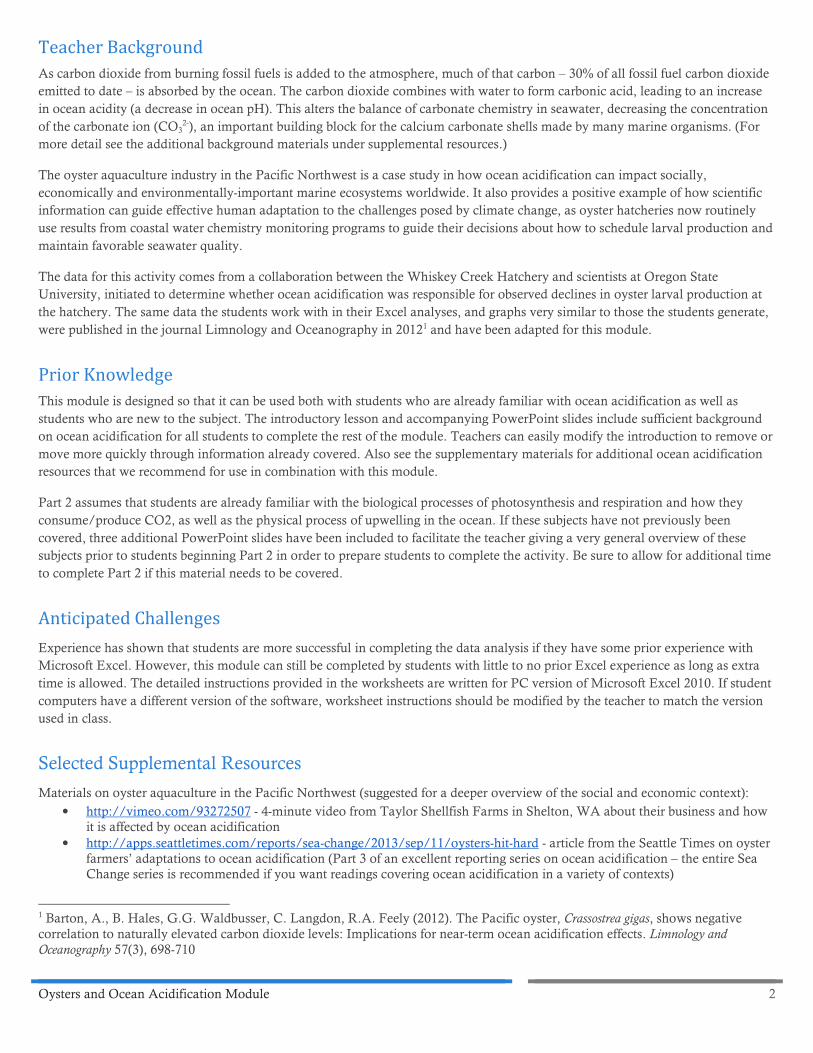
As carbon dioxide from burning fossil fuels is added to the atmosphere, much of that carbon – 30% of all fossil fuel carbon dioxide
emitted to date – is absorbed by the ocean. The carbon dioxide combines with water to form carbonic acid, leading to an increase
in ocean acidity (a decrease in ocean pH). This alters the balance of carbonate chemistry in seawater, decreasing the concentration
of the carbonate ion (CO32-), an important building block for the calcium carbonate shells made by many marine organisms. (For
more detail see the additional background materials under supplemental resources.)
The oyster aquaculture industry in the Pacific Northwest is a case study in how ocean acidification can impact socially,
economically and environmentally-important marine ecosystems worldwide. It also provides a positive example of how scientific
information can guide effective human adaptation to the challenges posed by climate change, as oyster hatcheries now routinely
use results from coastal water chemistry monitoring programs to guide their decisions about how to schedule larval production and
maintain favorable seawater quality.
The data for this activity comes from a collaboration between the Whiskey Creek Hatchery and scientists at Oregon State
University, initiated to determine whether ocean acidification was responsible for observed declines in oyster larval production at
the hatchery. The same data the students work with in their Excel analyses, and graphs very similar to those the students generate,
were published in the journal Limnology and Oceanography in 20121 and have been adapted for this module.
Prior Knowledge
This module is designed so that it can be used both with students who are already familiar with ocean acidification as well as
students who are new to the subject. The introductory lesson and accompanying PowerPoint slides include sufficient background
on ocean acidification for all students to complete the rest of the module. Teachers can easily modify the introduction to remove or
move more quickly through information already covered. Also see the supplementary materials for additional ocean acidification
resources that we recommend for use in combination with this module.
Part 2 assumes that students are already familiar with the biological processes of photosynthesis and respiration and how they
consume/produce CO2, as well as the physical process of upwelling in the ocean. If these subjects have not previously been
covered, three additional PowerPoint slides have been included to facilitate the teacher giving a very general overview of these
subjects prior to students beginning Part 2 in order to prepare students to complete the activity. Be sure to allow for additional time
to complete Part 2 if this material needs to be covered.
Anticipated Challenges
Experience has shown that students are more successful in completing the data analysis if they have some prior experience with
Microsoft Excel. However, this module can still be completed by students with little to no prior Excel experience as long as extra
time is allowed. The detailed instructions provided in the worksheets are written for PC version of Microsoft Excel 2010. If student
computers have a different version of the software, worksheet instructions should be modified by the teacher to match the version
used in class.
Selected Supplemental Resources
Materials on oyster aquaculture in the Pacific Northwest (suggested for a deeper overview of the social and economic context):
• http://vimeo.com/93272507 - 4-minute video from Taylor Shellfish Farms in Shelton, WA about their business and how
it is affected by ocean acidification
• http://apps.seattletimes.com/reports/sea-change/2013/sep/11/oysters-hit-hard - article from the Seattle Times on oyster
farmers’ adaptations to ocean acidification (Part 3 of an excellent reporting series on ocean acidification – the entire Sea
Change series is recommended if you want readings covering ocean acidification in a variety of contexts)
1 Barton, A., B. Hales, G.G. Waldbusser, C. Langdon, R.A. Feely (2012). The Pacific oyster, Crassostrea gigas, shows negative
correlation to naturally elevated carbon dioxide levels: Implications for near-term ocean acidification effects. Limnology and
Oceanography 57(3), 698-710

Oysters and Ocean Acidification Module 3
Additional teaching resources on ocean acidification:
• Institute for Systems Biology Ocean Acidification module (including links to a variety of outside content):
http://baliga.systemsbiology.net/drupal/education/?q=content/ocean-acidification-systems-approach-global-problem
• Virtual Urchin online lab from Stanford University: http://virtualurchin.stanford.edu/AcidOcean/AcidOcean.htm
• Center for Microbial Ecology Education and Research (C-MORE) Ocean Acidification science kit (hands-on labs focused
on corals): http://cmore.soest.hawaii.edu/education/teachers/science_kits/ocean_acid_kit.htm
• Ocean Carbon and Biogeochemistry (OCB) hands-on labs and demo: http://www.us-ocb.org/publications/OCB-
OA_labkit102609.pdf
Additional background on ocean acidification
• http://www.nanoos.org/education/learning_tools/oa/ocean_acidification.php - Recommended for an excellent
collection of additional ocean acidification-related websites and videos in right side bar. NANOOS also hosts a Visualization System for exploring ocean chemistry data from all around the Pacific Northwest.
• http://www.skepticalscience.com/docs/OA_not_OK_Mackie_McGraw_Hunter.pdf - Comprehensive but accessible
overview of the chemistry behind ocean acidification, also including a lot of additional context about the global carbon cycle
• http://www.aseachange.net/ - 83-minute documentary about ocean acidification, through the eyes of a retired teacher
concerned about the world his grandson will live in, who travels around the world to learn from scientists about their current research on ocean acidification (including great footage of field research). Not freely available, but can be rented/purchased from the website.
Assessment
If desired, students’ completed worksheets from this module could be collected and graded using the teacher key provided. For a
more formal assessment of student learning, exam questions based on the data and learning goals from this module are included in
the accompanying teacher materials.
Conducting the Lesson:
Preparation: Download both the student and teacher (key) versions of the Microsoft Excel data workbooks and accompanying
worksheets, as well as the PowerPoint slides. Prior to using the lesson in class, teachers should complete the entire module to
ensure they are prepared to answer student questions while completing the activity in class. Follow the worksheet instructions to
complete the calculations and graphing in the student version of the Microsoft Excel data workbook, and review the worksheet
answers provided in the key for teachers. The teacher should also review the accompanying PowerPoint slides to prepare to give
the introduction lecture with any necessary modifications to appropriately fit what has been previously covered in the course. Prior
to beginning Part 1 in class with the students, ensure that there are computers available with Microsoft Excel and that students will
have access to the student version of the data workbook (through a course website, Moodle, Edmodo, etc.).
Introduction: Teachers should select how to introduce this module based on the extent to which ocean acidification has been
previously covered in the course. A set of PowerPoint slides with accompanying lecture notes is provided with sufficient
information to provide an introduction for classes that have no prior exposure to the topic of ocean acidification. Teachers are
encouraged to modify these slides to fit their class. Slide #6 presents the equations that students will be expected to use in Part 1,
and slides #9-11 introduce the specific case of the oyster aquaculture industry in the Pacific Northwest that will be addressed in this
module, so it is recommended that these slides be used in all classes even if other portions of the introduction are omitted or
modified.
Please help us improve this activity! Prior to introducing the module, please have all students complete the pre-module survey.
Part 1: In this part, students compare their theoretical predictions with actual data showing how changes in the aragonite
saturation state of seawater affect larval oyster growth. Students should each individually or in pairs (depending on how many
computers are available) to work through Part 1 of the worksheet and complete the calculations and graphing using the Part 1 tab
of the Microsoft Excel workbook. The student worksheet gives detailed instructions for how to make the graph in Part 1. However,
it is strongly recommended that the teacher work through the worksheet and data analysis in advance using the same version of

Oysters and Ocean Acidification Module 4
Excel that the students will use in class in order to check that the instructions match the version of Excel that will be used and in
order to anticipate any student challenges.
Questions 1-4 ask students to demonstrate their understanding of the calcium carbonate dissolution reaction, how to calculate the
aragonite saturation state, and how to use that information to determine which direction the reaction will proceed. This
information will have already been covered in the introduction, but the teacher should observe the students’ answers to ensure that
they understand this material before proceeding.
While the students are completing Excel calculations and graphing, the teacher should circulate among the students to answer
questions and check for major errors in student progress. If many students are having problems with the same part, it is helpful to
have the Excel data loaded onto a computer connected to a projector so that you can demonstrate the correct procedure.
At the end of the class period, review the students’ responses to the worksheet as a class, including showing an example of the final
graph they each should have produced (in the accompanying PowerPoint slides) and asking students to share their interpretations
of the data in questions 8-9.
Part 2: In this part, students observe how diurnal photosynthesis and respiration and episodic upwelling control short-term
variability in seawater chemistry. Students should continue to work individually or in pairs through Part 2 of the worksheet,
completing the calculations and graphing in the Part 2 tab of the Microsoft Excel workbook. This part does not include graphic
illustrations of how to use Excel, although step-by-step procedures are still provided for graphing. If students have not previously
used functions in Excel, the teacher should briefly explain how to do this before they calculate the 1-day running mean in Question
4 using the AVERAGE function. It is again strongly recommended that the teacher work through the worksheet and data analysis
in advance of the students completing the activity in class.
At the end of the class period, again review the students’ responses to the worksheet as a class, including showing examples of the
final graphs they each should have produced (in the accompanying PowerPoint slides). Ask students to explain the role of
photosynthesis, respiration and upwelling in the data and ask them to share their ideas about how the hatchery can use this
information to change their practices. This is a good opportunity to conclude the class period on a positive note by explaining that
Pacific Northwest oyster hatcheries are in fact using this information to adapt their practices, and that the industry has recovered as
a result of improved scientific understanding and monitoring.
Note that three optional slides are provided in the PowerPoint for this part, which are designed for use in classes where students are
not already familiar with photosynthesis, respiration and/or upwelling to provide an overview of these concepts prior to students
beginning work on Part 2. These slides can be skipped if this material has already been covered.
Part 3: In this part, students calculate how ocean acidity is projected to change over the 21st century, compare this long-term
change to the existing variability in Netarts Bay that they described in Part 2 and predict how continued anthropogenic carbon
emissions will affect the oyster hatchery. Once students have completed the worksheet, review the students’ responses as a class
using the accompanying PowerPoint slides for additional figures showing projections of future changes to pH and aragonite
saturation state.
Please help us improve this activity! After completing the module, please have all students complete the post-module survey.
Mail the completed pre- and post-module surveys to:
Hilary Palevsky, School of Oceanography, Box 355351, University of Washington, Seattle WA 98195, [email protected]
Oysters and Ocean Acidification Module Student Worksheet Name__________________________
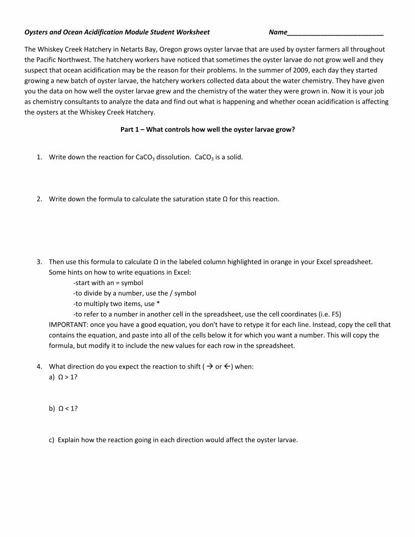
The Whiskey Creek Hatchery in Netarts Bay, Oregon grows oyster larvae that are used by oyster farmers all throughout
the Pacific Northwest. The hatchery workers have noticed that sometimes the oyster larvae do not grow well and they
suspect that ocean acidification may be the reason for their problems. In the summer of 2009, each day they started
growing a new batch of oyster larvae, the hatchery workers collected data about the water chemistry. They have given
you the data on how well the oyster larvae grew and the chemistry of the water they were grown in. Now it is your job
as chemistry consultants to analyze the data and find out what is happening and whether ocean acidification is affecting
the oysters at the Whiskey Creek Hatchery.
Part 1 – What controls how well the oyster larvae grow?
1. Write down the reaction for CaCO3 dissolution. CaCO3 is a solid.
2. Write down the formula to calculate the saturation state Ω for this reaction.
3. Then use this formula to calculate Ω in the labeled column highlighted in orange in your Excel spreadsheet.
Some hints on how to write equations in Excel:
-start with an = symbol
-to divide by a number, use the / symbol
-to multiply two items, use *
-to refer to a number in another cell in the spreadsheet, use the cell coordinates (i.e. F5)
IMPORTANT: once you have a good equation, you don't have to retype it for each line. Instead, copy the cell that
contains the equation, and paste into all of the cells below it for which you want a number. This will copy the
formula, but modify it to include the new values for each row in the spreadsheet.
4. What direction do you expect the reaction to shift ( � or ) when:
a) Ω > 1?
b) Ω < 1?
c) Explain how the reaction going in each direction would affect the oyster larvae.

5. Make a scatter plot in Excel, with Ω on the x-axis and
relative larval production on the y-axis.
a) Insert > Scatter > Select plot shown in this picture �
b) You'll get an empty plot. Move it off to the side.
c) Right click inside the plot > Select Data
d) You'll get a window that looks like this… click "Add":
e) In the next box that pops up, click in the box for Series X values. You will add the Ω data to plot on the X axis
by highlighting the Ω column (data only). A new box will pop up while you are highlighting the data, but then
disappear once you have finished.
NOTE: you'll see the Series X field fill in based
on the column of cells you selected in orange.
f) To fill in the Series Y values, delete the “={1}”
Then you will add the Relative Larval Production data to
plot on the Y axis by highlighting the data in the Relative
larval production column (data only), as above.
g) Click under “Series name:” at the top and type in a name for your graph (think about what the data is about to
show you and choose a clear, descriptive title!)
h) Click OK then OK and you should see a plot!

6. Next, fit a trend line through these data.
a) Click on the graph, find "Layout" tab at top, then "Trend Line" and select "Linear Trendline"
7. Look at the trendline and your data and describe the relationship between Ω and relative larval production.
*Relative larval production (RLP) is a measurement of how much the population of larvae grew between when
they were 48 hours old and when they reached 1-2 weeks old. If RLP>0, the population grew, if RLP<0, it got
smaller, and if RLP = 0, the population stayed the same size.
8. Using the trend line on your graph,
a) Above what value of Ω is relative larval production > 0?
b) Is this what you expected? Why or why not?
c) Why might the oyster larvae have responded differently to changes in Ω than you had expected?
9. Summarize your analysis for the managers of the Whiskey Creek Hatchery: Is ocean acidification causing
problems for their oyster larvae? Explain your reasoning.
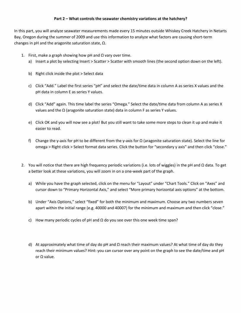
Part 2 – What controls the seawater chemistry variations at the hatchery?
In this part, you will analyze seawater measurements made every 15 minutes outside Whiskey Creek Hatchery in Netarts
Bay, Oregon during the summer of 2009 and use this information to analyze what factors are causing short-term
changes in pH and the aragonite saturation state, Ω.
1. First, make a graph showing how pH and Ω vary over time.
a) Insert a plot by selecting Insert > Scatter > Scatter with smooth lines (the second option down on the left).
b) Right click inside the plot > Select data
c) Click “Add.” Label the first series “pH” and select the date/time data in column A as series X values and the
pH data in column E as series Y values.
d) Click “Add” again. This time label the series “Omega.” Select the date/time data from column A as series X
values and the Ω (aragonite saturation state) data in column F as series Y values.
e) Click OK and you will now see a plot! But you still want to take some more steps to clean it up and make it
easier to read.
f) Change the y-axis for pH to be different from the y-axis for Ω (aragonite saturation state). Select the line for
omega > Right click > Select format data series. Click the button for “secondary y axis” and then click “close.”
2. You will notice that there are high frequency periodic variations (i.e. lots of wiggles) in the pH and Ω data. To get
a better look at these variations, you will zoom in on a one-week part of the graph.
a) While you have the graph selected, click on the menu for “Layout” under “Chart Tools.” Click on “Axes” and
cursor down to “Primary Horizontal Axis,” and select “More primary horizontal axis options” at the bottom.
b) Under “Axis Options,” select “fixed” for both the minimum and maximum. Choose any two numbers seven
apart within the initial range (e.g. 40000 and 40007) for the minimum and maximum and then click “close.”
c) How many periodic cycles of pH and Ω do you see over this one week time span?
d) At approximately what time of day do pH and Ω reach their maximum values? At what time of day do they
reach their minimum values? Hint: you can cursor over any point on the graph to see the date/time and pH
or Ω value.
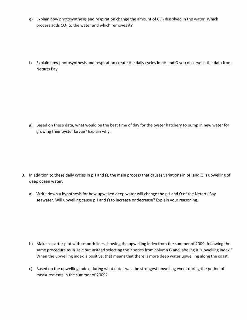
e) Explain how photosynthesis and respiration change the amount of CO2 dissolved in the water. Which
process adds CO2 to the water and which removes it?
f) Explain how photosynthesis and respiration create the daily cycles in pH and Ω you observe in the data from
Netarts Bay.
g) Based on these data, what would be the best time of day for the oyster hatchery to pump in new water for
growing their oyster larvae? Explain why.
3. In addition to these daily cycles in pH and Ω, the main process that causes variations in pH and Ω is upwelling of
deep ocean water.
a) Write down a hypothesis for how upwelled deep water will change the pH and Ω of the Netarts Bay
seawater. Will upwelling cause pH and Ω to increase or decrease? Explain your reasoning.
b) Make a scatter plot with smooth lines showing the upwelling index from the summer of 2009, following the
same procedure as in 1a-c but instead selecting the Y series from column G and labeling it “upwelling index.”
When the upwelling index is positive, that means that there is more deep water upwelling along the coast.
c) Based on the upwelling index, during what dates was the strongest upwelling event during the period of
measurements in the summer of 2009?

d) Make a new graph showing variations in temperature and salinity over time to compare to the graph of pH
and Ω. Follow the same directions as in #1, but this time with temperature on the first Y series and salinity as
the second Y series. (Hint: to see the data clearly, you may need to adjust the scale on the vertical (Y) axes.)
e) How do salinity and temperature change during the upwelling event you identified in part c)? Explain why
these changes occur.
4. To see whether there are changes in pH and Ω due to upwelling in these data, you will graph the 1-day running
mean of pH and Ω over the entire measurement period.
a) What is the confounding daily signal we want to separate out by taking the 1-day running mean of pH and Ω
over the entire measurement period?
NOTE: If you want to see what pH and Ω look like over the entire measurement period without taking the 1-
day running mean, make a copy of your graph of pH and Ω from questions 1-2 and change the time scale on
the x-axis back to “Auto,” following the same procedure as in 2b-2c.
b) In the top row under “pH 1-day mean,” use the AVERAGE function to calculate the average of all pH data
over the first day of the measurement period (type “=AVERAGE(“, then highlight all the data from the pH
column for the first day, then type “)” and hit enter).
c) Follow the same procedure using the AVERAGE function to calculate the average of all Ω data over the first
day of the measurement period in the top row under “Ω 1-day mean.”
d) Then copy these two cells with the AVERAGE equations and paste into all the orange highlighted cells down
to the bottom, filling all the cells with the correct formula and calculating the running mean of pH and Ω
throughout the entire measurement period.
e) Follow the same procedure as in question 1 to graph pH and Ω, but this time use the running mean data you
just calculated to plot on the Y-axes.
f) What trend do you observe in pH and Ω during the upwelling event? Is this consistent with your hypothesis
from part a)?
g) Based on these data, what recommendations would you give to the oyster hatchery for how to use NOAA’s
Upwelling Index forecast in deciding when to pump in new water for growing their oyster larvae? Explain
your reasoning.
Low future
emissions
High future
emissions
Part 3 – future projections and recommendations for the oyster hatchery
Now that you have analyzed what is happening at the oyster hatchery today, your final job is to predict how the
hatchery will be affected by future changes in ocean chemistry and provide a summary of your findings and
recommendations for the hatchery operators.
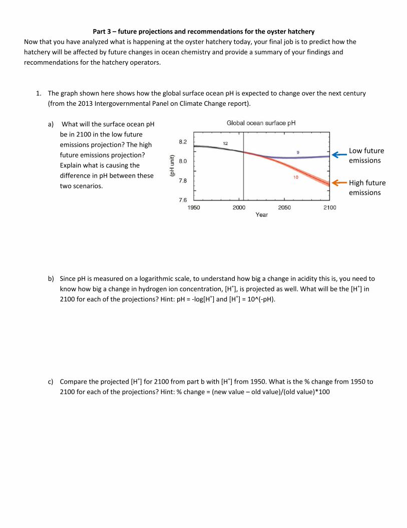
1. The graph shown here shows how the global surface ocean pH is expected to change over the next century
(from the 2013 Intergovernmental Panel on Climate Change report).
a) What will the surface ocean pH
be in 2100 in the low future
emissions projection? The high
future emissions projection?
Explain what is causing the
difference in pH between these
two scenarios.
b) Since pH is measured on a logarithmic scale, to understand how big a change in acidity this is, you need to
know how big a change in hydrogen ion concentration, [H+], is projected as well. What will be the [H
+] in
2100 for each of the projections? Hint: pH = -log[H+] and [H
+] = 10^(-pH).
c) Compare the projected [H+] for 2100 from part b with [H
+] from 1950. What is the % change from 1950 to
2100 for each of the projections? Hint: % change = (new value – old value)/(old value)*100

2. Now you will predict how Whiskey Creek Hatchery will be affected by the changes projected by the IPCC from
now to 2100.
a) What is the range of pH found in Netarts Bay in 2009? (Use the MIN and MAX functions with the data in the
Excel spreadsheets to find this.)
b) What range of pH would you predict for Netarts Bay in 2100 for the low emissions projection? The high
emissions projection? Assume the pH at Netarts Bay will change at the same rate as the global surface
ocean.
c) How do you predict Ω will change between now and 2100? Explain your reasoning.
d) How do you expect these future changes in ocean chemistry will affect the oyster hatchery?

Pre-Module Survey (Front and Back!)
Please fill out this survey to help improve future students’ learning. This survey is anonymous and will
NOT influence your grades. It is OK to guess the correct answer. The information you provide will help
science educators understand if this activity is effective.
1. Explain how increasing CO2 in the atmosphere is changing ocean chemistry.
a) It creates acid rain, so when precipitation falls over the ocean, it increases the ocean’s
acidity.
b) It increases concentrations of CO2 in the ocean, which reacts to remove the O2 from the
water and makes it difficult for fish and other animals to breathe.
c) It increases concentrations of CO2 in the ocean, which reacts with water to form carbonic
acid, increasing the ocean’s acidity.
d) All of the above
2. How much has ocean acidity increased since the pre-industrial period (1750 to today)?
a) 0.1%
b) 11%
c) 26%
d) 151%
3. Explain how organisms with calcium carbonate shells are affected by ocean acidification.
a) Ocean acidification contaminates shellfish and makes them dangerous for people to eat.
b) It decreases the concentrations of the ions in the water that the organisms need to
precipitate their shells.
c) Organisms are more vulnerable to predation because they are left living without their shells.
d) All of the above
4. Which of the following processes affect the acidity of surface seawater along the Pacific
Northwest coast?
a) Upwelling of deep ocean water
b) Respiration by marine organisms
c) Photosynthesis by marine organisms
d) All of the above
5. If a friend asked you to explain ocean acidification, how confident would you be with your
answer?
a) Not at all confident, or wouldn’t be able to answer
b) Slightly confident in a basic explanation
c) Moderately confident
d) Fairly confident in a full explanation
e) Very confident, and able to give a detailed explanation
6. How important do you consider the problem of ocean acidification?
a) Not at all important
b) Slightly important
c) Important
d) Fairly important
e) Very important
Thank you for completing the survey!

Post-Module Survey (Front and Back!)
Please fill out this survey to help improve future students’ learning. This survey is anonymous and will
NOT influence your grades. It is OK to guess the correct answer. The information you provide will help
science educators understand if this activity is effective.
1. Explain how increasing CO2 in the atmosphere is changing ocean chemistry.
a) It creates acid rain, so when precipitation falls over the ocean, it increases the ocean’s
acidity.
b) It increases concentrations of CO2 in the ocean, which reacts to remove the O2 from the
water and makes it difficult for fish and other animals to breathe.
c) It increases concentrations of CO2 in the ocean, which reacts with water to form carbonic
acid, increasing the ocean’s acidity.
d) All of the above
2. How much has ocean acidity increased since the pre-industrial period (1750 to today)?
a) 0.1%
b) 11%
c) 26%
d) 151%
3. Explain how organisms with calcium carbonate shells are affected by ocean acidification.
a) Ocean acidification contaminates shellfish and makes them dangerous for people to eat.
b) It decreases the concentrations of the ions in the water that the organisms need to
precipitate their shells.
c) Organisms are more vulnerable to predation because they are left living without their shells.
d) All of the above
4. Which of the following processes affect the acidity of surface seawater along the Pacific
Northwest coast?
a) Upwelling of deep ocean water
b) Respiration by marine organisms
c) Photosynthesis by marine organisms
d) All of the above
5. If a friend asked you to explain ocean acidification, how confident would you be with your
answer?
a) Not at all confident, or wouldn’t be able to answer
b) Slightly confident in a basic explanation
c) Moderately confident
d) Fairly confident in a full explanation
e) Very confident, and able to give a detailed explanation
6. How important do you consider the problem of ocean acidification?
a) Not at all important
b) Slightly important
c) Important
d) Fairly important
e) Very important
7. How useful was analyzing data from the Oregon oyster hatchery in helping you learn about
ocean acidification? What did you like best about this activity? What do you think could be
improved?
Thank you for completing the survey!