optimization by using differential evolution (de) dr. p. n...
TRANSCRIPT

Optimization by Using Differential Evolution (DE)
Dr. P. N. Suganthan, EEE, NTU, Singapore
Some Software Resources Available from:
http://www.ntu.edu.sg/home/epnsugan
IEEE TENCON 2016
MBS, Singapore, 22nd Nov. 2016
OverviewI. Introduction to Real Variable Optimization & DE
II. Single Objective Optimization
III. Constrained Optimization
IV. Multi-objective Optimization
V. Multimodal Optimization
VI. Expensive Optimization
VII. Large Scale Optimization
VIII. Dynamic Optimization
But, first a little publicity ….
S. Das, S. S. Mullick, P. N. Suganthan, "Recent Advances in Differential Evolution - An
Updated Survey," Swarm and Evolutionary Computation, Vol. 27, pp. 1-30, 2016.
S. Das and P. N. Suganthan, “Differential Evolution: A Survey of the State-of-the-Art”,
IEEE Trans. on Evolutionary Computation, 15(1):4 – 31, Feb. 2011. 2

Ensemble / Adaptive Methods for Evolutionary
Algorithms:
http://www.ntu.edu.sg/home/epnsugan/index_files/EEAs-
EOAs.htm
Optimization Benchmark Test Problems Surveys
Codes of several of our research publications
available from
http://www.ntu.edu.sg/home/epnsugan
(limited to our own publications & CEC Competitions)
The reason for selecting differential evolution (DE)
is due to its superior performance in all CEC
competitions.
3

Consider submitting to
SWEVO journal
dedicated to the EC-SI
fields
SCI Indexed from Vol.
1, Issue 1.
2016 IFs:
2 years = 2.9
5 years= 5.7

Overview
I. Introduction to Real Variable Optimization & DE
II. Single Objective Optimization
III. Constrained Optimization
IV. Multi-objective Optimization
V. Multimodal Optimization
VI. Expensive Optimization
VII. Large Scale Optimization
VIII. Dynamic Optimization
5

General Thoughts: NFL (No Free Lunch Theorem)
• Glamorous Name for Commonsense?
– Over a large set of problems, it is impossible to find a single best algorithm
– DE with Cr=0.90 & Cr=0.91 are two different algorithms Infinite algos.
– Practical Relevance: Is it common for a practicing engineer to solve several
practical problems at the same time? (NO)
– Academic Relevance: Very High
Other NFL Like Commonsense Scenarios
Panacea: A medicine to cure all diseases (No need for doctors), Amrita the nectar
of immortal perfect life …
Silver bullet: in politics … (you can search these on internet)
Jack of all trades, but master of none
If you have a hammer all problems look like nails 6

General Thoughts: Convergence
• What is exactly convergence in the context of EAs & SAs ?
– The whole population reaching a single point (within a tolerance)
– Single point based search methods & convergence …
• In the context of real world problem solving, are we going to reject a
good solution because the population hasn’t converged ?
• Good to have all population members converging to the global
solution OR good to have high diversity even after finding the
global optimum ? (Fixed Computational budget Scenario)
• What we do not want to have:
For example, in the context of PSO, we do not want to have chaotic oscillations
c1 + c2 > 4.1+
7

General Thoughts: Algorithmic Parameters
• Good to have many algorithmic parameters / operators ?
• Possible to be robust against parameter / operator variations ?
• What are Reviewers’ preferences ?
• Or good to have several parameters that can be adaptively
tuned on the fly to achieve top performance on diverse
problems?
• If NFL says that a single algorithm is not the best for a very
large set of problems, then good to have many algorithmic
parameters & operators to be adapted for different problems !!
CEC 2015 Competitions: “Learning-Based Optimization”
Similar Literature: Thomas Stützle, Holger Hoos, …8

General Thoughts: Nature Inspired Methods
• Good to mimic closely natural phenomena?
• Honey bees solve only one problem (gathering honey). Can this
(ABC or BCO) be the best approach for solving all problems?
• NFL & Nature inspired methods.
• Nature inspired methods & lack of crossover.
9

Differential Evolution
• A stochastic population-based algorithm for continuous function optimization (Storn and Price, 1995)
• Finished 3rd at the First International Contest on Evolutionary Computation, Nagoya, 1996 (icsi.berkley.edu/~storn)
• Outperformed several variants of GA and PSO over a wide variety of numerical benchmarks over past several years.
• Continually exhibited remarkable performance in competitions on different kinds of optimization problems like dynamic, multi-objective, constrained, and multi-modal problems held under IEEE congress on Evolutionary Computation (CEC) conference series.
• Very easy to implement in any standard programming language.
• Very few control parameters (typically three for a standard DE) and their effects on the performance have been well studied.
• Spatial complexity is very low as compared to some of the most competitive continuous optimizers like CMA-ES.
10

DE is an Evolutionary Algorithm
This Class also includes GA, Evolutionary Programming and Evolutionary Strategies
Initialization Mutation Recombination Selection
Basic steps of an Evolutionary Algorithm
11
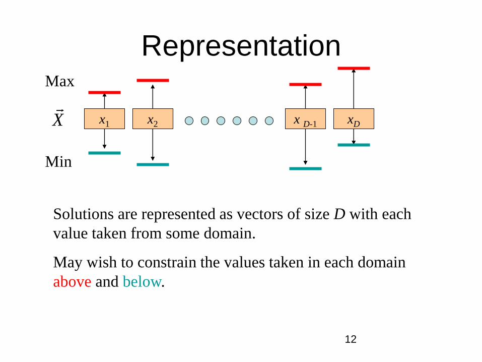
Representation
Min
Max
May wish to constrain the values taken in each domain
above and below.
x1 x2 x D-1 xD
Solutions are represented as vectors of size D with each
value taken from some domain.
X
12

Maintain Population - NP
x1,1 x2,1 x D-1,1 xD,1
x1,2 x2,2 xD-1,2 xD,2
x1,NP x2,NP x D-1,NP xD, NP
We will maintain a population of size NP
1X
2X
NPX
13

The population size NP
1) The influence of NP on the performance of DE is yet to be extensively studied and
fully understood.
2) Storn and Price have indicated that a reasonable value for NP could be chosen
between 5D and 10D (D being the dimensionality of the problem).
3) Brest and Maučec presented a method for gradually reducing population size of
DE. The method improves the efficiency and robustness of the algorithm and can
be applied to any variant of DE.
4) But, recently, all best performing DE variants used populations ~50-100 for
dimensions from 50D to 1000D for the following scalability Special Issue:
F. Herrera M. Lozano D. Molina, "Test Suite for the Special Issue of Soft Computing
on Scalability of Evolutionary Algorithms and other Metaheuristics for Large Scale
Continuous Optimization Problems". Available: http://sci2s.ugr.es/eamhco/CFP.php.
14

Different values are instantiated for each i and j.
Max and Min are the upper – lower bounds.
Min
Max
x2,i,0 x D-1,i,0 xD,i,0x1,i,0
, ,0 ,min , ,max ,min[0,1] ( )j i j i j j jx x rand x x
0.42 0.22 0.78 0.83
Initialization Mutation Recombination Selection
, [0,1]i jrand
iX
15

Initialization Mutation Recombination Selection
For each vector select three other parameter vectors randomly.
Add the weighted difference of two of the parameter vectors to the
third to form a donor vector (most commonly seen form of
DE-mutation):
The scaling factor F is a constant from (0, 2)
Self-referential Mutation
).(,,,,
321 GrGrGrGi iii XXFXV
16

Example of formation of donor vector over two-
dimensional constant cost contours
Constant cost contours of
Sphere function
17
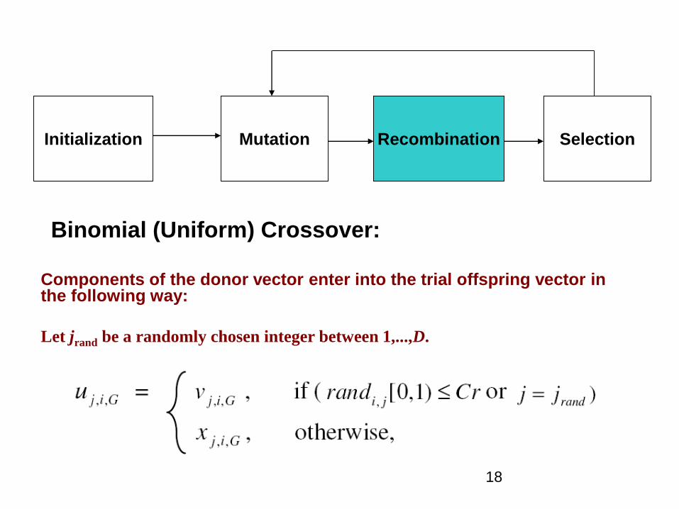
Initialization Mutation Recombination Selection
Components of the donor vector enter into the trial offspring vector in the following way:
Let jrand be a randomly chosen integer between 1,...,D.
Binomial (Uniform) Crossover:
18

An Illustration of Binomial Crossover in 2-D Parametric Space:
Three possible trial vectors:
19

Exponential (two-point modulo) Crossover:
Pseudo-code for choosing L:
where the angular brackets Ddenote a modulo function with modulus D.
First choose integers n (as starting point) and L (number of components the
donor actually contributes to the offspring) from the interval [1,D]
20
Exploits linkages among neighboring decision variables. If benchmarks have this
feature, it performs well. Similarly, for real-world problems with neighboring linkages.
Binomial is more commonly used crossover operator.
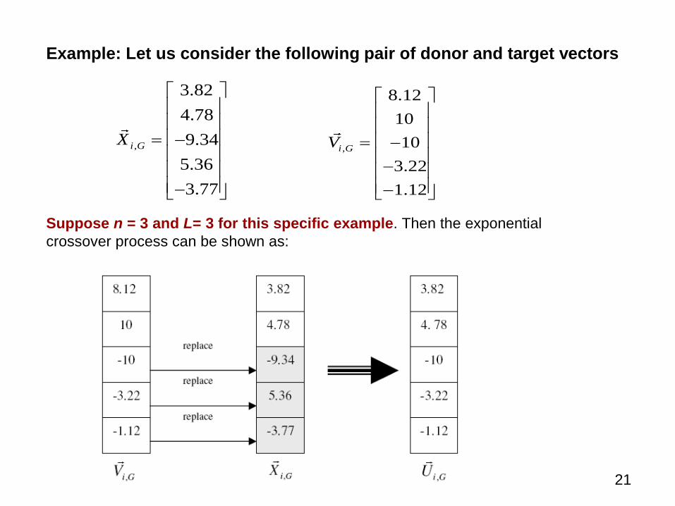
Example: Let us consider the following pair of donor and target vectors
,
3.82
4.78
9.34
5.36
3.77
i GX
,
8.12
10
10
3.22
1.12
i GV
Suppose n = 3 and L= 3 for this specific example. Then the exponential
crossover process can be shown as:
21

Initialization Mutation Recombination Selection
“Survival of the fitter” principle in selection: The trial
offspring vector is compared with the target (parent)
vector and the one with a better fitness is admitted to the
next generation population.
1, GiX
,,GiU
)()( ,, GiGi XfUf
if
,,GiX
if )()( ,, GiGi XfUf
Importance of parent-mutant crossover & parent-
offspring competition-based selection
22

An Example of Optimization by DE
Consider the following two-dimensional function
f (x, y) = x2+y2 The minima is at (0, 0)
Let’s start with a population of 5 candidate solutions randomly initiated in the
range (-10, 10)
X1,0 = [2, -1] X2,0 = [6, 1] X3,0 = [-3, 5] X4,0 = [-2, 6]
X5,0= [6,-7]
For the first vector X1, randomly select three other vectors say X2,
X4 and X5
Now form the donor vector as, V1,0 = X2,0+F. (X4,0 – X5,0)
1,0
6 2 6 0.40.8
1 6 7 10.4V
23

Now we form the trial offspring vector by exchanging
components of V1,0 with the target vector X1,0
Let rand[0, 1) = 0.6. If we set Cr = 0.9,
since 0.6 < 0.9, u1,1,0 = V1,1,0 = - 0.4
Again next time let rand[0, 1) = 0.95 > Cr
Hence u1,2,0 = x1,2,0 = - 1
So, finally the offspring is 1,0
0.4
1U
Fitness of parent:
f (2, -1) = 22 + (-1)2 = 5
Fitness of offspring
f (-0.4, -1) = (-0.4)2 + (-1)2 = 1.16
Hence the parent is replaced by offspring at G = 124

Population
at G = 0
Fitness
at G = 0
Donor vector
at G = 0
Offspring Vector
at G = 0
Fitness of
offspring at
G = 1
Evolved
population at
G = 1
X1,0 =
[2,-1]
5 V1,0
=[-0.4,10.4]
U1,0
=[-0.4,-1]
1.16 X1,1
=[-0.4,-1]
X2,0=
[6, 1]
37 V2,0
=[1.2, -0.2]
U2,0
=[1.2, 1]
2.44 X2,1
=[1.2, 1]
X3,0=
[-3, 5]
34 V3,0
=[-4.4, -0.2]
U3,0
=[-4.4, -0.2]
19.4 X3,1
=[-4.4, -0.2]
X4,0=
[-2, 6]
40 V4,0
=[9.2, -4.2 ]
U4,0
=[9.2, 6 ]
120.64 X4,1
=[-2, 6 ]
X5,0=
[6, 7]
85 V5,0
=[5.2, 0.2]
U5,0
=[6, 0.2]
36.04 X5,1
=[6, 0.2]
25

Locus of the fittest solution: DE working on 2D Sphere Function
26

Locus of the fittest solution: DE working on 2D Rosenbrock Function
27

“DE/rand/1”: )).()(()()(321
tXtXFtXtV iii rrri
“DE/best/1”:
“DE/target-to-best/1”:
“DE/best/2”:
“DE/rand/2”:
)).()(.()()(21
tXtXFtXtV ii rrbesti
)),()(.())()(.()()(21
tXtXFtXtXFtXtV ii rribestii
)).()(.())()(.()()(4321
tXtXFtXtXFtXtV iiii rrrrbesti
)).()(.())()(.()()(54321
21 tXtXFtXtXFtXtV iiiii rrrrri
Five most frequently used DE mutation schemes
The general convention used for naming the various mutation strategies is
DE/x/y/z, where DE stands for Differential Evolution, x represents a string
denoting the vector to be perturbed, y is the number of difference vectors
considered for perturbation of x, and z stands for the type of crossover being
used (exp: exponential; bin: binomial) 28
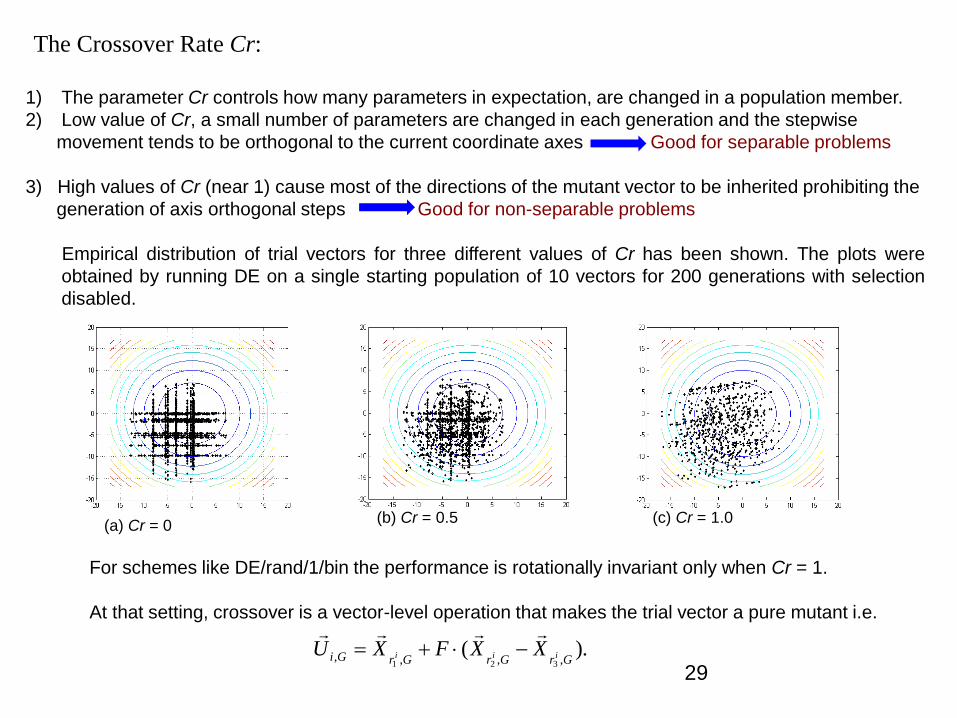
The Crossover Rate Cr:
1) The parameter Cr controls how many parameters in expectation, are changed in a population member.
2) Low value of Cr, a small number of parameters are changed in each generation and the stepwise
movement tends to be orthogonal to the current coordinate axes Good for separable problems
3) High values of Cr (near 1) cause most of the directions of the mutant vector to be inherited prohibiting the
generation of axis orthogonal steps Good for non-separable problems
Empirical distribution of trial vectors for three different values of Cr has been shown. The plots were
obtained by running DE on a single starting population of 10 vectors for 200 generations with selection
disabled.
(a) Cr = 0(b) Cr = 0.5 (c) Cr = 1.0
For schemes like DE/rand/1/bin the performance is rotationally invariant only when Cr = 1.
At that setting, crossover is a vector-level operation that makes the trial vector a pure mutant i.e.
).(,,,,
321 GrGrGrGi iii XXFXU
29

OverviewI. Introduction to Real Variable Optimization & DE
II. Single Objective Optimization
III. Constrained Optimization
IV. Multi-objective Optimization
V. Multimodal Optimization
VI. Expensive Optimization
VII. Large Scale Optimization
VIII. Dynamic Optimization
30
-31-
Importance of Population Topologies• In population based algorithms, population members exchange
information between them.
• Single population topology permits all members to exchange
information among themselves – the most commonly used.
• Other population topologies have restrictions on information
exchange between members – the oldest is island model
• Restrictions on information exchange can slow down the
propagation of information from the best member in the population
to other members (i.e. single objective global optimization)
• Hence, this approach
– slows down movement of other members towards the best member(s)
– Enhances the exploration of the search space
– Beneficial when solving multi-modal problems
As global version of the PSO converges fast, many topologies were
Introduced to slow down PSO …

PSO with Neighborhood Operator
Presumed to be the oldest paper to consider distance based
neighborhoods for real-parameter optimization.
Lbest is selected from the members that are closer (w.r.t.
Euclidean distance) to the member being updated.
Initially only a few members are within the neighborhood (small
distance threshold) and finally all members are in the n’hood.
Island model and other static/dynamic neighborhoods did not
make use of Euclidean distances, instead just the indexes of
population members.
Our recent works are extensively making use of distance based
neighborhoods to solve many classes of problems.
32
P. N. Suganthan, “Particle swarm optimizer with neighborhood
operator,” in Proc. Congr. Evol. Comput., Washington, DC, pp.1958–
1962, 1999.
Two Subpopulations with Heterogeneous
Ensembles & Topologies
Proposed for balancing exploration and exploitation capabilities
Population is divided into exploration / exploitation sub-poplns Exploration Subpopulation group uses exploration oriented ensemble
of parameters and operators
Exploitation Subpopulation group uses exploitation oriented ensemble
of parameters and operators.
• Topology allows information exchange only from explorative subpopulation
to exploitation sub-population. Hence, diversity of exploration popln not
affected even if exploitation popln converges.
• The need for memetic algorithms in real parameter optimization: Memetic
algorithms were developed because we were not able to have an EA or SI to be
able to perform both exploitation and exploration simultaneously. This 2-popln
topology allows with heterogeneous information exchange.
33

Two Subpopulations with Heterogeneous
Ensembles & Topologies
Sa.EPSDE realization (for single objective Global):
N. Lynn, R Mallipeddi, P. N. Suganthan, “Differential Evolution with Two
Subpopulations," LNCS 8947, SEMCCO 2014.
2 Subpopulations CLPSO (for single objective Global)N. Lynn, P. N. Suganthan, “Comprehensive Learning Particle Swarm Optimization with
Heterogeneous Population Topologies for Enhanced Exploration and Exploitation,”
Swarm and Evolutionary Computation, 2015.
Neighborhood-Based Niching-DE: Distance based neighborhood forms local
topologies while within each n’hood, we employ exploration-exploitation
ensemble of parameters and operators.
S. Hui, P N Suganthan, “Ensemble and Arithmetic Recombination-Based Speciation Differential
Evolution for Multimodal Optimization,” IEEE T. Cybernetics, Online since Mar 2015.
10.1109/TCYB.2015.2394466
B-Y Qu, P N Suganthan, J J Liang, "Differential Evolution with Neighborhood Mutation for
Multimodal Optimization," IEEE Trans on Evolutionary Computation, DOI:
10.1109/TEVC.2011.2161873. (Supplementary file), Oct 2012. (Codes Available: 2012-TEC-
DE-niching)34

Adaptations
• Self-adaptation: parameters and operators are evolved by
coding them together with solution vector
• Separate adaptation based on performance: operators
and parameter values yielding improved solutions are
rewarded.
• 2nd approach is more successful and frequently used in
DE.
35
Self-Adaptive DE (SaDE) (Qin et al., 2009)
• Includes both control parameter adaptation and strategy adaptation
Strategy Adaptation:
Four effective trial vector generation strategies: DE/rand/1/bin, DE/rand-to-
best/2/bin, DE/rand/2/bin and DE/current-to-rand/1 are chosen to constitute
a strategy candidate pool.
For each target vector in the current population, one trial vector generation
strategy is selected from the candidate pool according to the probability
learned from its success rate in generating improved solutions (that can
survive to the next generation) within a certain number of previous
generations, called the Learning Period (LP).
A. K. Qin, V. L. Huang, and P. N. Suganthan, Differential evolution algorithm
with strategy adaptation for global numerical optimization", IEEE Trans. on
Evolutionary Computation, 13(2):398-417, April, 2009.36

SaDE (Contd..)
Control Parameter Adaptation:
1) NP is left as a user defined parameter.
2) A set of F values are randomly sampled from normal distribution
N(0.5, 0.3) and applied to each target vector in the current
population.
3) CR obeys a normal distribution with mean value and standard
deviation Std =0.1, denoted by where is
initialized as 0.5.
4) SaDE gradually adjusts the range of CR values for a given problem
according to previous CR values that have generated trial vectors
successfully entering the next generation.
mCR
),( StdCRN m mCR
37

Population Size Reduction
• Evolutionary algorithms are expected to explore the
search space in the early stages
• In the final stages of search, exploitation of previously
found good regions takes place.
• For exploration of the whole search space, we need a
large population while for exploration, we need a small
population size.
• Hence, population size reduction will be effective for
evolutionary algorithms.
38

JADE (Zhang and Sanderson, 2009)
1) Uses DE/current-to-pbest strategy as a less greedy generalization of the DE/current-to-
best/ strategy. Instead of only adopting the best individual in the DE/current-to-best/1
strategy, the current-to-pbest/1 strategy utilizes the information of other good solutions.
Denoting p
GbestX ,
as a randomly chosen vector from the top 100p% individuals of the current population,
DE/current-to-pbest/1 without external archive:1 2
, , , , , ,( ) ( )i i
p
i G i G i best G i G i r G r GV X F X X F X X
2) JADE can optionally make use of an external archive (A), which stores the recently explored inferior
solutions. In case of DE/current-to-pbest/1 with archive, , , and are selected from the
current population P, but is selected from
GiX ,
p
GbestX ,
Gr iX
,1
2 ,ir GX AP
J. Zhang, and A. C. Sanderson, “JADE: Adaptive differential evolution with
optional external archive”, IEEE Transactions on Evolutionary Computation,
Vol. 13, Issue 5, Page(s): 945-958, Oct. 2009.
39
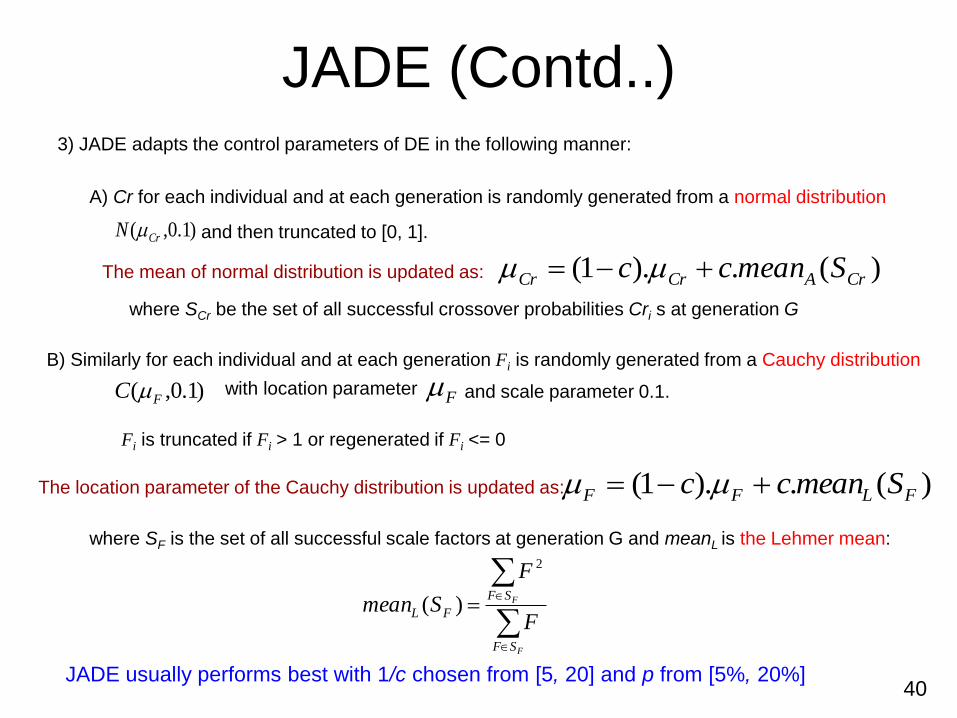
JADE (Contd..)3) JADE adapts the control parameters of DE in the following manner:
A) Cr for each individual and at each generation is randomly generated from a normal distribution
)1.0,( CrN and then truncated to [0, 1].
The mean of normal distribution is updated as: )(.).1( CrACrCr Smeancc
where SCr be the set of all successful crossover probabilities Cri s at generation G
B) Similarly for each individual and at each generation Fi is randomly generated from a Cauchy distribution
)1.0,( FC with location parameterF and scale parameter 0.1.
The location parameter of the Cauchy distribution is updated as:
Fi is truncated if Fi > 1 or regenerated if Fi <= 0
)(.).1( FLFF Smeancc
where SF is the set of all successful scale factors at generation G and meanL is the Lehmer mean:
F
F
SF
SF
FLF
F
Smean
2
)(
JADE usually performs best with 1/c chosen from [5, 20] and p from [5%, 20%] 40
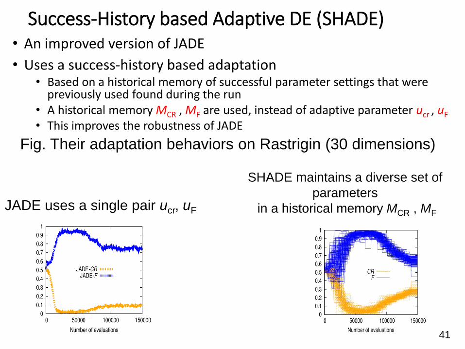
Success-History based Adaptive DE (SHADE) • An improved version of JADE
• Uses a success-history based adaptation• Based on a historical memory of successful parameter settings that were
previously used found during the run• A historical memory MCR , MF are used, instead of adaptive parameter ucr , uF
• This improves the robustness of JADE
Fig. Their adaptation behaviors on Rastrigin (30 dimensions)
JADE uses a single pair ucr, uF
SHADE maintains a diverse set of
parameters
in a historical memory MCR , MF
41

SHADE
• The weighted Lehmer mean (in CEC’14 ver.) values of SCR and SF , which are successful parameters for each generation, are stored in a historical memory MCR and MF
• CRi and Fi are generated by selecting an index ri randomly from [1, memory size H]
• Example: if selected index ri = 2• CRi = NormalRand(0.87, 0.1)• Fi = CauchyRand(0.52, 0.1)
42

Example of memory update in SHADE
• The contents of both memories are initialized to 0.5 and the index counter is set 1
• The CRi and Fi values used by successful individuals are recorded in SCR and SF
• At the end of the generation, the contents of memory are updated by the mean values of SCR and SF
• The index counter is incremented
• Even if SCR , SF for some particular generation contains a poor set of values, the parameters stored in memory from previous generations cannot be directly, negatively impacted
• If the index counter exceeds the memory size H, the index counter wraps around to 1 again 43

Deterministic population reduction methods
• General Policy for Evolutionary Algorithms• Explorative search is appropriate for estimating the promising
regions
• Exploitative search is appropriate for finding the higher precision solutions
• Deterministic population reduction methods• They use a large population size as initial population and
reduce its size
• This mechanism makes EA more robust and effective.
“Evaluating the performance of SHADE on CEC 2013 benchmark problems”, Ryoji Tanabe and Alex Fukunaga, The University of Tokyo, Japan (Codes-Results available, as SHADE_CEC2013)
L-SHADE in CEC 2014: “Improving the Search Performance of SHADE Using Linear Population Size Reduction,” By Ryoji Tanabe and Alex S. Fukunaga 44
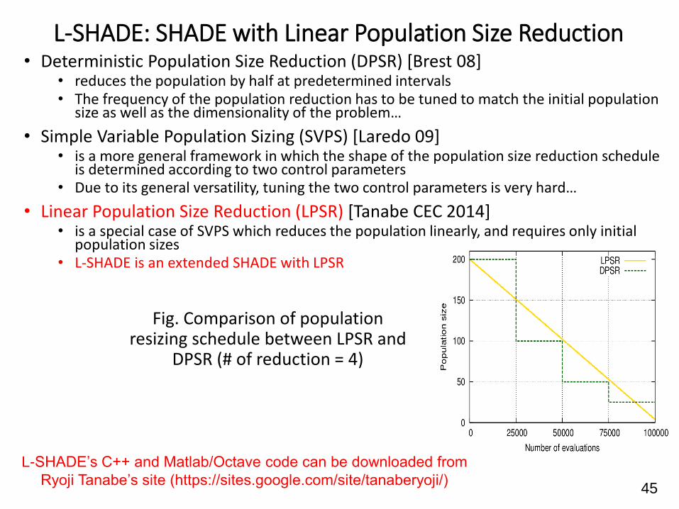
L-SHADE: SHADE with Linear Population Size Reduction
Fig. Comparison of population resizing schedule between LPSR and
DPSR (# of reduction = 4)
• Deterministic Population Size Reduction (DPSR) [Brest 08]• reduces the population by half at predetermined intervals • The frequency of the population reduction has to be tuned to match the initial population
size as well as the dimensionality of the problem…
• Simple Variable Population Sizing (SVPS) [Laredo 09]• is a more general framework in which the shape of the population size reduction schedule
is determined according to two control parameters • Due to its general versatility, tuning the two control parameters is very hard…
• Linear Population Size Reduction (LPSR) [Tanabe CEC 2014]• is a special case of SVPS which reduces the population linearly, and requires only initial
population sizes• L-SHADE is an extended SHADE with LPSR
L-SHADE’s C++ and Matlab/Octave code can be downloaded from
Ryoji Tanabe’s site (https://sites.google.com/site/tanaberyoji/)45

Ensemble Methods
• Ensemble methods are commonly used for pattern
recognition (PR), forecasting, and prediction, e.g. multiple
predictors.
• Not commonly used in Evolutionary algorithms ...
There are two advantages in EA (compared to PR):
1. In PR, we have no idea if a predicted value is correct or
not. In EA, we can look at the objective values and make
some conclusions.
2. Sharing of function evaluation among ensembles possible.
46

Ensemble of Parameters and Mutation and Crossover Strategies in DE (EPSDE )
Motivation
o Empirical guidelines
o Adaptation/self-adaptation (different variants)
o Optimization problems (Ex: uni-modal & multimodal)
o Fixed single mutation strategy & parameters – may not be the best always
Implementation
o Contains a pool of mutation strategies & parameter values
o Compete to produce successful offspring population.
o Candidate pools must be restrictive to avoid unfavorable influences
o The pools should be diverse
R. Mallipeddi, P. N. Suganthan, Q. K. Pan and M. F. Tasgetiren, “Differential Evolution
Algorithm with ensemble of parameters and mutation strategies,”
Applied Soft Computing, 11(2):1679–1696, March 2011.
47
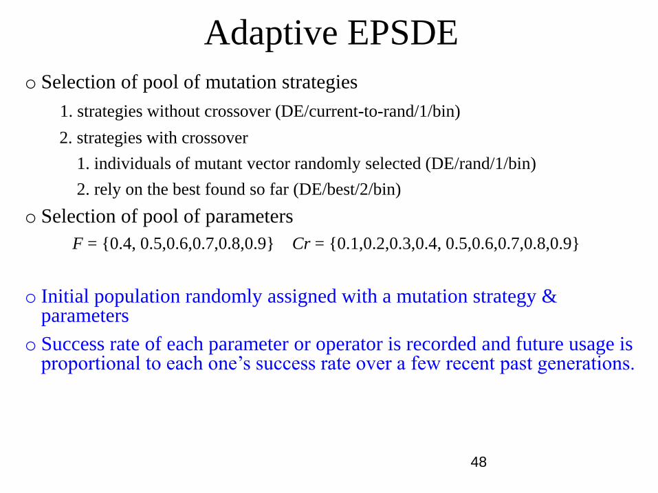
Adaptive EPSDE
o Selection of pool of mutation strategies
1. strategies without crossover (DE/current-to-rand/1/bin)
2. strategies with crossover
1. individuals of mutant vector randomly selected (DE/rand/1/bin)
2. rely on the best found so far (DE/best/2/bin)
o Selection of pool of parameters
F = {0.4, 0.5,0.6,0.7,0.8,0.9} Cr = {0.1,0.2,0.3,0.4, 0.5,0.6,0.7,0.8,0.9}
o Initial population randomly assigned with a mutation strategy & parameters
o Success rate of each parameter or operator is recorded and future usage is proportional to each one’s success rate over a few recent past generations.
48

Overview
I. Introduction to Real Variable Optimization & DE
II. Single Objective Optimization
III. Constrained Optimization
IV. Multi-objective Optimization
V. Multimodal Optimization
VI. Expensive Optimization
VII. Large Scale Optimization
VIII. Dynamic Optimization
49

-50-
Single Objective Constrained Optimization
Currently DE with local Search and Ensemble of Constraint handling are competitive.
CEC'06 Special Session / Competition on Evolutionary Constrained Real Parameter single objective optimization
CEC10 Special Session / Competition on Evolutionary Constrained Real Parameter single objective optimization
E Mezura-Montes, C. A. Coello Coello, "Constraint-handling in nature-inspired numerical optimization: Past, present and future", Vol. 1, No. 4, pp. 173-194, Swarm and Evolutionary Computation, Dec 2011.
R. Mallipeddi, P. N. Suganthan, "Efficient Constraint Handling for Optimal Reactive Power Dispatch Problem," Swarm and Evolutionary Computation, Vol. 5, pp. 28–36, Aug. 2012. (Codes Available: 2012-SWEVO-Cnostr-Handl-4-power)

Constraint Handling Methods
• Many optimization problems in science and engineering involve constraints. The presence of constraints reduces the feasible region and complicates the search process.
• Evolutionary algorithms (EAs) always perform unconstrained search.
• When solving constrained optimization problems, they require additional mechanisms to handle constraints
-51-
-52-
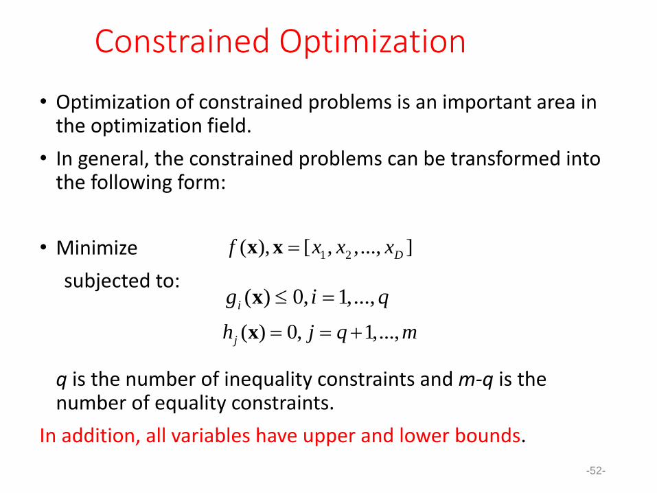
Constrained Optimization
• Optimization of constrained problems is an important area in the optimization field.
• In general, the constrained problems can be transformed into the following form:
• Minimize
subjected to:
q is the number of inequality constraints and m-q is the number of equality constraints.
In addition, all variables have upper and lower bounds.
1 2( ), [ , ,..., ]Df x x xx x
( ) 0, 1,...,jh j q m x
( ) 0, 1,...,ig i q x

-53-
Constrained Optimization
• For convenience, the equality constraints can be transformed into inequality form:
where is the allowed tolerance.
• Then, the constrained problems can be expressed as
Minimize
subjected to
| ( ) | 0jh x
1 2( ), [ , ,..., ]Df x x xx x
1,..., 1,... 1,..., 1,...
( ) 0, 1,..., ,
( ) ( ), ( ) ( )
j
q q q m q m
G j m
G g G h
x
x x x x
-54-
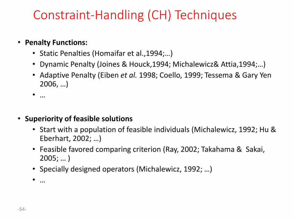
Constraint-Handling (CH) Techniques
• Penalty Functions:
• Static Penalties (Homaifar et al.,1994;…)
• Dynamic Penalty (Joines & Houck,1994; Michalewicz& Attia,1994;…)
• Adaptive Penalty (Eiben et al. 1998; Coello, 1999; Tessema & Gary Yen 2006, …)
• …
• Superiority of feasible solutions
• Start with a population of feasible individuals (Michalewicz, 1992; Hu & Eberhart, 2002; …)
• Feasible favored comparing criterion (Ray, 2002; Takahama & Sakai, 2005; … )
• Specially designed operators (Michalewicz, 1992; …)
• …

-55-
Constraint-Handling (CH) Techniques
• Separation of objective and constraints• Co-evolution methods (Coello, 2000a)
• Multi-objective optimization techniques (Coello, 2000b; Mezura-Montes & Coello, 2002;… )
• Feasible solution search followed by optimization of objective (Venkatraman & Gary Yen, 2005)
• …
• While most CH techniques are modular (i.e. we can pick one CH technique and one search method independently), there are also CH techniques embedded as an integral part of the EA.

Superiority of Feasible
• In SF when two solutions Xi and Xj are compared, Xi is regarded superior to Xj under the following conditions:
1. Xi is feasible and Xj is not.
2. Xi and Xj are both feasible and Xi has smaller objective value (for minimization problems) than Xj.
3. Xi and Xj are both infeasible, but Xi has a smaller overall constraint violation.
-56-

Superiority of Feasible (SF)
• Therefore, in SF feasible ones are always considered better than the infeasible ones.
• Two infeasible solutions are compared based on their overall constraint violations only, while two feasible solutions are compared based on their objective function values only.
• Comparison of infeasible solutions on the constraint violation aims to push the infeasible solutions to feasible region, while comparison of two feasible solutions on the objective value improves the overall solution.
-57-
Self-Adaptive Penalty (SP) • In self adaptive penalty function method two types of penalties are added to
each infeasible individual to identify the best infeasible individuals in the current population.
• The amount of the added penalties is controlled by the number of feasible individuals currently present in the combined population.
• If there are a few feasible individuals, a higher amount of penalty is added to infeasible individuals with a higher amount of constraint violation.
• On the other hand, if there are several feasible individuals, then infeasible individuals with high fitness values will have small penalties added to their fitness values.
• These two penalties will allow the algorithm to switch between finding more feasible solutions and searching for the optimum solution at anytime during the search process.
-58-

Epsilon Constraint handling (EC)
• The relaxation of the constraints is controlled by using the parameter
• High quality solutions for problems with equality constraints can be obtained by proper control of the parameter.
•The parameter is initialized using:
where is the top th individual in the initialized population after sorting w. r. t. constraint violation.
)()0( X
X
-59-

Epsilon Constraint Handling (EC)
•The is updated until the generation counter kreaches the control generation , after which is set to zero to obtain solutions with no constraint violation.
•The recommended parameter settings are:
c
cp
c
cTk
Tk
T
k
k
0 ,
,0
1)0()(
cT
]8.0,1.0[ maxmax TTTc ]10 ,2[cp
-60-
Ensemble of Constraint Handling Techniques (ECHT)
• According to the no free lunch theorem (NFL) , no single state-of-the-art constraint handling technique can outperform all others on every problem.
• Each constrained problem would be unique in terms of the ratio between feasible search space and the whole search space, multi-modality and the nature of constraint functions.
• Evolutionary algorithms are stochastic in nature. Hence the evolution paths can be different in every run even when the same problem is solved by using the same algorithm implying different CH can be efficient in different runs.
R. Mallipeddi, P. N. Suganthan, “Ensemble of Constraint Handling Techniques”, IEEE Trans. on Evolutionary Computation, Vol. 14, No. 4, pp. 561 - 579 , Aug. 2010
-61-

Ensemble of Constraint
Handling Techniques (ECHT): MOTIVATION
• Therefore, depending on several factors such as the ratio between feasible search space and the whole search space, multi-modality of the problem, nature of equality / inequality constraints, the chosen EA, global exploration/local exploitation stages of the search process, different constraint handling methods can be effective during different stages of the search process.
• Hence, solving a particular constrained problem requires numerous trial-and-error runs to choose a suitable constraint handling technique and to fine tune the associated parameters. Even after this, the NFL theorem says that one well tuned method may not be able to solve all problems instances satisfactorily.
-62-

ECHT
• Each constraint handling technique has its own population and parameters.
• Each population corresponding to a constraint handling method produces its offspring.
• The parent population corresponding to a particular constraint handling method not only competes with its own offspring population but also with offspring population of the other constraint handling methods.
• Due to this, an offspring produced by a particular constraint handling method may be rejected by its own population, but could be accepted by the populations of other constraint handling methods.
-63-
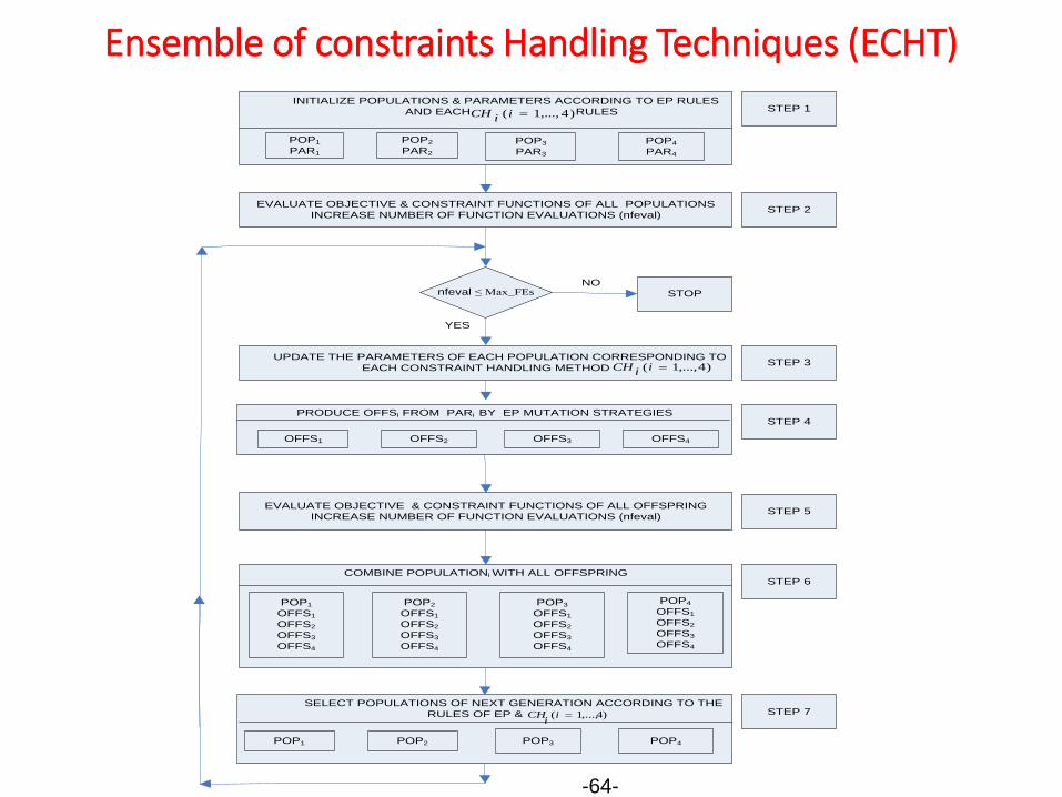
Ensemble of constraints Handling Techniques (ECHT)
INITIALIZE POPULATIONS & PARAMETERS ACCORDING TO EP RULES
AND EACH RULES
POP1
PAR1
POP2
PAR2
POP3
PAR3
EVALUATE OBJECTIVE & CONSTRAINT FUNCTIONS OF ALL POPULATIONS
INCREASE NUMBER OF FUNCTION EVALUATIONS (nfeval)
nfeval ≤ Max_FEs STOP
PRODUCE OFFSi FROM PARi BY EP MUTATION STRATEGIES
OFFS1 OFFS2 OFFS3
EVALUATE OBJECTIVE & CONSTRAINT FUNCTIONS OF ALL OFFSPRING
INCREASE NUMBER OF FUNCTION EVALUATIONS (nfeval)
COMBINE POPULATIONi WITH ALL OFFSPRING
POP1
OFFS1
OFFS2
OFFS3
OFFS4
POP2
OFFS1
OFFS2
OFFS3
OFFS4
POP3
OFFS1
OFFS2
OFFS3
OFFS4
SELECT POPULATIONS OF NEXT GENERATION ACCORDING TO THE
RULES OF EP &
POP1 POP2 POP3
POP4
PAR4
)4,...,1( iiCH
NO
OFFS4
POP4
OFFS1
OFFS2
OFFS3
OFFS4
)4,...,1( ii
CH
YES
POP4
UPDATE THE PARAMETERS OF EACH POPULATION CORRESPONDING TO
EACH CONSTRAINT HANDLING METHOD )4,...,1( iiCH
STEP 1
STEP 2
STEP 3
STEP 4
STEP 5
STEP 6
STEP 7
-64-

ECHT
• Hence, in ECHT every function call is utilized effectively. If the evaluation of objective / constraint functions is computationally expensive, more constraint handling methods can be included in the ensemble to benefit more from each function call.
• And if a particular constraint handling technique is best suited for the search method and the problem during a point in the search process, the offspring population produced by the population of that constraint handling method dominates the other and enters other populations too.
• In the subsequent generations, these superior offspring will become parents in other populations too.
-65-
ECHT
• Therefore, ECHT transforms the burden of choosing a particular constraint handling technique and tuning the associated parameter values for a particular problem into an advantage.
• If the constraint handling methods selected to form an ensemble are similar in nature then the populations associated with each of them may lose diversity and the search ability of ECHT may be deteriorated.
• Thus the performance of ECHT can be improved by selecting diverse and competitive constraint handling methods.
-66-

ECHT
• The constraint handling methods used in the ensemble are
1.Superiority of Feasible (SF)
2.Self-Adaptive penalty (SP)
3.Stochastic Ranking (SR)
4.Epsilon Constraint handling (EC)
Detailed Results in:
R. Mallipeddi, P. N. Suganthan, “Ensemble of Constraint Handling Techniques”, IEEE Trans. on Evolutionary Computation, Vol. 14, No. 4, pp. 561 - 579 , Aug. 2010
-67-
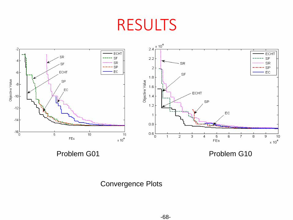
RESULTS
Problem G01 Problem G10
Convergence Plots
-68-

Variable reduction strategy (VRS)
• Although EAs can treat optimization problems as black-boxes (e.g., academic benchmarks), evidences showing that the exploitation of specific problem domain knowledge can improve the problem solving efficiency.
• Technically, optimization can be viewed a process that an algorithm act on a problem. To promote this process, we canEnhance the capability of optimization algorithms,Make use of the domain knowledge hidden in the problem to
reduce its complexity.
• We may thinkWhether there exists general domain knowledge?How to use such knowledge?
Guohua Wu , Witold Pedrycz, P. N. Suganthan, Rammohan Mallipeddi, “A Variable Reduction Strategy for Evolutionary Algorithms Handling Equality Constraints,” Applied soft computing, 37 (2015): 774-786 69
IDEAS IN VRS
• We utilize the domain knowledge of equality optimal conditions (EOCs) of optimization problems. EOCs are expressed by equation systems;
EOCs have to be satisfied for optimal solutions;
EOCs are necessary conditions;
EOCs are general.
• Equality constraints are much harder to be completely satisfied when an EA is taken as the optimizer.
• The equality constraints of constrained optimization problems (COPs) are treated as EOCs to reduce variables and eliminate equality constraints.
70

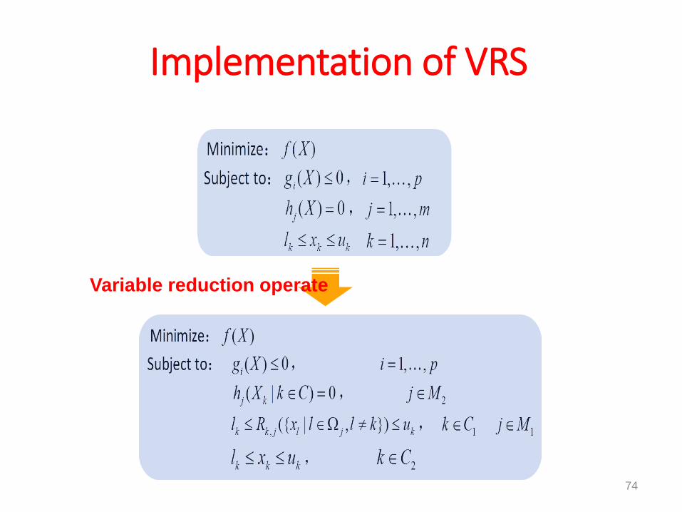
Implementation of VRS
Minimize: ( )f X
Subject to: ( ) 0ig X , 1, ,i p
( ) 0jh X , 1, ,j m
k k kl x u , 1, ,k n
| ( ) | 0jh X
71

Implementation of VRS
Assume j denotes the collection of variables involved in equality constraint ( ) 0jh X
From ( ) 0jh X (1 j m ), if we can obtain a relationship
, ({ | , })k k j l jx R x l l k
kx can be actually calculated by relationship ,k jR and the values of variables in { | , }l jx l l k
Moreover, equality constraint ( )jh X is always satisfied.
As a result, both ( )jh X and kx are eliminated.
72
Implementation of VRS
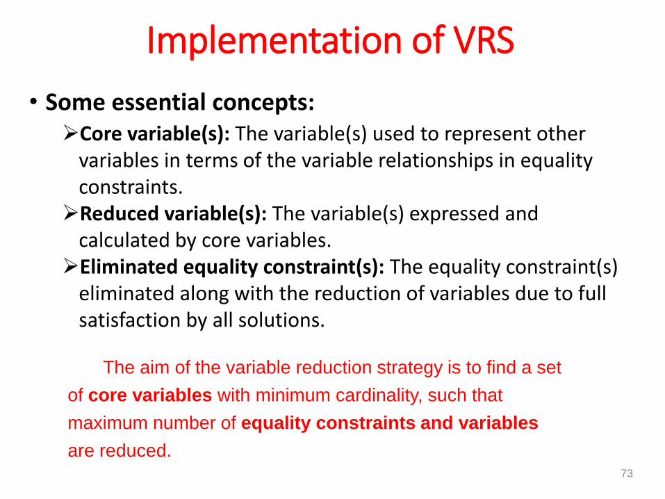
• Some essential concepts:Core variable(s): The variable(s) used to represent other
variables in terms of the variable relationships in equality constraints.
Reduced variable(s): The variable(s) expressed and calculated by core variables.
Eliminated equality constraint(s): The equality constraint(s) eliminated along with the reduction of variables due to full satisfaction by all solutions.
The aim of the variable reduction strategy is to find a set
of core variables with minimum cardinality, such that
maximum number of equality constraints and variables
are reduced.73
Implementation of VRS
Variable reduction operate
74

• Naïve example, considering:
• We can obtain the variable relationship and substitute it into original problem, then we get
2 2
1 2
1 2
1 2
min
2
0 5,0 5
x x
x x
x x
2 12x x
2
1 1
1
min 2 4 4
0 2
x x
x
Implementation of VRS
75

• Solution space before and after the variable reduction process
0 0.5 1 1.5 22
2.2
2.4
2.6
2.8
3
3.2
3.4
3.6
3.8
4
x1
f
(a) Original solution
space
(b) Solution after VRS.
Implementation of VRS
76
Implementation of VRS
77

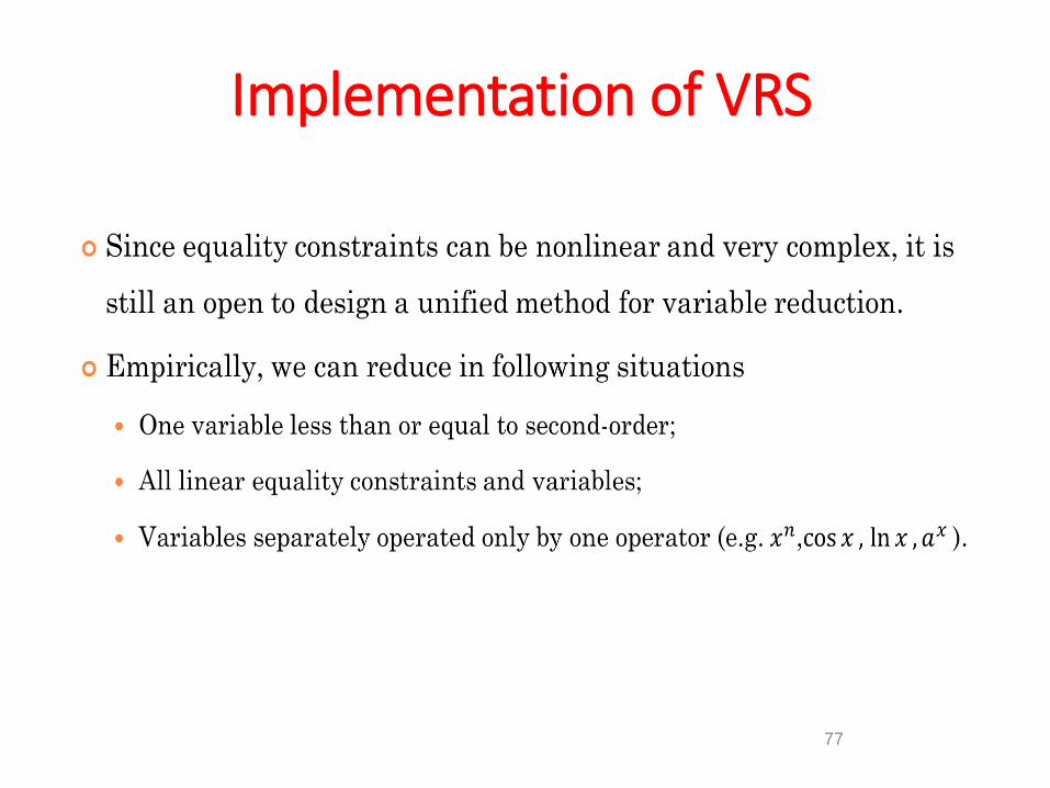
• A formal method automatically reducing linear equality constraint and variables.
• Matrix form of linear equality constraint
• Expand it and we get
AX b
11 1 12 2 1 1
21 1 22 2 2 2
1 1 2 2
n n
n n
m m mn n m
a x a x a x b
a x a x a x b
a x a x a x b
m n
IMPLEMENTATION OF VRS
78

• We can transform the expanded form into
• Let
• We have
11 1 12 2 1 1 1, 1 1 1, 2 2 1,
21 1 22 2 2 2 2, 1 1 2, 2 2 2,
1 1 2 2
( )
( )
m m m m m m n n
m m m m m m n n
m m
a x a x a x b a x a x a x
a x a x a x b a x a x a x
a x a x
, 1 1 , 2 2 ,( )mm m m m m m m m m m n na x b a x a x a x
11 1
1
m
m mm
a a
A
a a
1
2
m
x
xX
x
1 1, 1 1 1, 2 2 1,
2 2, 1 1 2, 2 2 2,
, 1 1 , 2 2 ,
( )
( )
( )
m m m m n n
m m m m n n
m m m m m m m m n n
b a x a x a x
b a x a x a xb
b a x a x a x
A X b 1( )X A b
X is reduced and all linear equality constraints are eliminated.

Experimental results• Impact of VRS on the number of variables and equality constraints of the
Benchmark COPs Problem Original COP COP after ECVRS
g03 Variables 10 9
Equality Const. 1 0
g05 Variables 4 1
Equality Const. 3 0
g11 Variables 2 1
Equality Const. 1 0
g13 Variables 5 2
Equality Const. 3 0
g14 Variables 10 7
Equality Const. 3 0
g15 Variables 3 2
Equality Const. 1 0
g17 Variables 6 2
Equality Const. 4 0
g21 Variables 7 2
Equality Const. 5 0
g22 Variables 22 3
Equality Const. 19 0
g23 Variables 9 5
Equality Const. 4 0
80

Experimental resultsProblems
ECHT-DE ECHT-DE-
ECVRS
ECHT-EP ECHT-EP
-ECVRS
SF-DE SF-DE
-ECVRS
EC-EP EC-EP
-ECVRS
g03
Best -1.0005 -1.0000 -1.0005 -1.0000 -1.0005 -1.0000 -1.0005 -1.0000
Mean -1.0005 -1.0000 -1.0005 -1.0000 -1.0005 -1.0000 -1.0005 -1.0000
Worst -1.0005 -1.0000 -1.0004 -1.0000 -1.0005 -1.0000 -1.0005 -1.0000
Std 2.3930e-10 2.1612e-16 1.6026e-05 8.7721e-14 3.3013e-16 2.8816e-16 1.4728e-06 2.8658e-16
Violation 3.6892e-04 0.0 2.6684e-04 0.0 2.6631e-04 0.0 1.0000e-04 0.0
g05
Best 5.1265e+03 5.1265e+03 5.1265e+03 5.1265e+03 5.1265e+03 5.1265e+03 5.1265e+03 5.1265e+03
Mean 5.1265e+03 5.1265e+03 5.1265e+03 5.1265e+03 5.1265e+03 5.1265e+03 5.1265e+03 5.1265e+03
Worst 5.1265e+03 5.1265e+03 5.1265e+03 5.1265e+03 5.1265e+03 5.1265e+03 5.1266e+03 5.1265e+03
Std 2.0865e-12 9.33125e-13 2.0212e-07 9.3312e-13 1.9236e-12 9.3312e-13 3.2214e−02 9.3312e-13
Violation 3.0543e-04 0.0 4.6534e-04 0.0 8.0598e-04 0.0 6.0558e-04 0.0
g11
Best 7.4990e-01 7.5000e-01 7.4990e-01 7.5000e-01 7.4990e-01 7.5000e-01 7.4990e-01 7.5000e-01
Mean 7.4990e-01 7.5000e-01 7.4990e-01 7.5000e-01 7.4990e-01 7.5000e-01 7.4990e-01 7.5000e-01
Worst 7.4990e-01 7.5000e-01 7.4990e-01 7.5000e-01 7.4990e-01 7.5000e-01 7.4990e-01 7.5000e-01
Std 1.1390e-16 0.0 1.1390e-16 0.0 1.1390e-16 0.0 2.1630e-09 0.0
Violation 1.0989e-04 0.0 1.0000e-05 0.0 1.0539e-04 0.0 9.9999e-05 0.0
g13
Best 5.3942e-02 5.3949e-02 5.3942e-02 5.3949e-02 5.3942e-02 5.3949e-02 5.4137e-02 5.3949e-02
Mean 1.3124e-01 5.3949e-02 5.3942e-02 5.3949e-02 3.5288e-01 5.3949e-02 5.4375e-02 5.3949e-02
Worst 4.4373e-01 5.3949e-02 5.3942e-02 5.3949e-02 4.6384e-01 5.3949e-02 5.6346e-02 5.3949e-02
Std 1.5841e-01 6.3675e-18 5.3942e-02 1.5597e-17 1.4745e-01 7.9594e-18 6.3439e-03 1.2834e-17
Violation 3.9935e-04 0.0 5.0444e-09 0.0 1.0000e-04 0.0 2.7237e-02 0.0
g14
Best -4.7765e+01 -4.7761e+01 -4.7761e+01 -4.7761e+01 -4.7765e+01 -4.7761e+01 -4.7765e+01 -4.7761e+01
Mean -4.7765e+01 -4.7761e+01 -4.7703e+01 -4.7761e+01 -4.7765e+01 -4.7761e+01 -4.5142e+01 -4.7706e+01
Worst -4.7765e+01 -4.7761e+01 -4.7405e+01 -4.7761e+01 -4.7765e+01 -4.7761e+01 -4.3762e+01 -4.7361e+01
Std 2.1625e-05 1.6703e-14 7.8687e-02 2.9722e-12 1.8728e-14 3.7355e-14 7.3651e-01 2.1542e-02
Violation 2.9212e-04 0.0 2.9999e-04 0.0 3.0000e-004 0.0 2.9999e-04 0.0
g15
Best 9.6172e+02 9.6172e+02 9.6172e+02 9.6172e+02 9.6172e+02 9.6172e+02 9.6233e+02 9.6172e+02
Mean 9.6172e+02 9.6172e+02 9.6172e+02 9.6172e+02 9.6172e+02 9.6172e+02 9.6248e+02 9.6172e+02
Worst 9.6172e+02 9.6172e+02 9.6172e+02 9.6172e+02 9.6172e+02 9.6172e+02 9.6265e+02 9.6172e+02
Std 5.8320e-13 1.1664e-13 6.1830e-13 1.1664e-13 5.8320e-13 1.1664e-13 7.3719e+01 1.1664e-13
Violation 1.9995e-04 0.0 1.9999e-04 0.0 2.0000e-04 0.0 2.1737e-01 0.0
g17
Best 8.8535e+03 8.8535e+03 8.8535e+03 8.8535e+03 8.8535e+03 8.8535e+03 9.1573e+03 8.8535e+03
Mean 8.8535e+03 8.8535e+03 8.8535e+03 8.8535e+03 8.8757e+03 8.8535e+03 9.1791e+03 8.8535e+03
Worst 8.8535e+03 8.8535e+03 8.8535e+03 8.8535e+03 8.9439e+03 8.8535e+03 9.2005e+03 8.8535e+03
Std 3.7324e-12 1.8662e-12 2.0301e-08 1.8662e-12 3.8524e+01 1.8662e-12 1.2346e+01 1.8662e-12
Violation 3.2953e-04 0.0 2.6943e-04 0.0 1.7744e-04 0.0 3.1295e-04 0.0
g21
Best 1.9372e+02 1.9379e+02 1.9372e+02 1.9379e+02 1.9372e+02 1.9379e+02 1.9872e+02 1.9379e+02
Mean 1.9984e+02 1.9379e+02 1.9498e+02 1.9379e+02 2.0682e+02 1.9379e+02 2.3474e+02 1.9379e+02
Worst 3.1604e+02 1.9379e+02 2.0661e+02 1.9379e+02 3.2470e+02 1.9379e+02 2.7589e+02 1.9379e+02
Std 2.7351e+01 2.8632e-12 3.8129e+00 3.8765e-12 4.0314e+01 6.8507e-10 2.6621e+01 3.8625e-12
Violation 4.0195e-04 0.0 4.8585e-04 0.0 9.9999e-05 0.0 3.0432e-03 0.0
g22
Best 1.8857e+03 2.3637e+02 3.9184e+02 2.3637e+02 3.9643e+03 2.3637e+02 2.2545e+03 2.3637e+02
Mean 1.0158e+04 2.3637e+02 7.7786e+02 2.3637e+02 1.3812e+04 2.3637e+02 1.2854e+04 2.3637e+02
Worst 1.7641e+04 2.3637e+02 1.4844e+03 2.3637e+02 1.9205e+04 2.3637e+02 1.6328e+04 2.3637e+02
Std 4.2890e+03 1.4580e-13 3.0970e+02 2.2875e-13 5.0860e+03 7.3769e-14 3.2582e+03 1.9875e-13
Violation 4.1562e+03 0.0 2.7186e+03 0.0 1.3192e+04 0.0 4.156e+03 0.0
g23
Best -3.9072e+02 -4.0000e+02 -3.4556e+02 -4.0000e+02 -3.9158e+02 -4.0000e+02 −3.8625e+02 -4.0000e+02
Mean -3.6413e+02 -4.0000e+02 -3.0952e+02 -4.0000e+02 -2.4367e+02 -4.0000e+02 −3.4864e+02 -4.0000e+02
Worst -2.3426e+02 -4.0000e+02 -2.5807e+02 -4.0000e+02 -1.0004e+02 -4.0000e+02 −2.7235e+02 -4.0000e+02
Std 3.4129e+01 1.1664e-13 2.5417e+01 4.8217e-09 1.9487e+01 0.0 2.3654e+01 1.7496e-13
Violation 3.5951e-04 0.0 1.7373e-04 0.0 2.5635e-02 0.0 8.8827e-02 0.0
81

Experimental results
Problems ECHT-DE ECHT-DE-
ECVRS
ECHT-EP ECHT-EP
-ECVRS
SF-DE SF-DE
-ECVRS
EC-EP EC-EP
-ECVRS
g03
Best -1.0005 -1.0000 -1.0005 -1.0000 -1.0005 -1.0000 -1.0005 -1.0000
Mean -1.0005 -1.0000 -1.0005 -1.0000 -1.0005 -1.0000 -1.0005 -1.0000
Worst -1.0005 -1.0000 -1.0004 -1.0000 -1.0005 -1.0000 -1.0005 -1.0000
Std 2.3930e-10 2.1612e-16 1.6026e-05 8.7721e-14 3.3013e-16 2.8816e-16 1.4728e-06 2.8658e-16
Violation 3.6892e-04 0.0 2.6684e-04 0.0 2.6631e-04 0.0 1.0000e-04 0.0
g05
Best 5.1265e+03 5.1265e+03 5.1265e+03 5.1265e+03 5.1265e+03 5.1265e+03 5.1265e+03 5.1265e+03
Mean 5.1265e+03 5.1265e+03 5.1265e+03 5.1265e+03 5.1265e+03 5.1265e+03 5.1265e+03 5.1265e+03
Worst 5.1265e+03 5.1265e+03 5.1265e+03 5.1265e+03 5.1265e+03 5.1265e+03 5.1266e+03 5.1265e+03
Std 2.0865e-12 9.33125e-13 2.0212e-07 9.3312e-13 1.9236e-12 9.3312e-13 3.2214e−02 9.3312e-13
Violation 3.0543e-04 0.0 4.6534e-04 0.0 8.0598e-04 0.0 6.0558e-04 0.0
g11
Best 7.4990e-01 7.5000e-01 7.4990e-01 7.5000e-01 7.4990e-01 7.5000e-01 7.4990e-01 7.5000e-01
Mean 7.4990e-01 7.5000e-01 7.4990e-01 7.5000e-01 7.4990e-01 7.5000e-01 7.4990e-01 7.5000e-01
Worst 7.4990e-01 7.5000e-01 7.4990e-01 7.5000e-01 7.4990e-01 7.5000e-01 7.4990e-01 7.5000e-01
Std 1.1390e-16 0.0 1.1390e-16 0.0 1.1390e-16 0.0 2.1630e-09 0.0
Violation 1.0989e-04 0.0 1.0000e-05 0.0 1.0539e-04 0.0 9.9999e-05 0.0
g13
Best 5.3942e-02 5.3949e-02 5.3942e-02 5.3949e-02 5.3942e-02 5.3949e-02 5.4137e-02 5.3949e-02
Mean 1.3124e-01 5.3949e-02 5.3942e-02 5.3949e-02 3.5288e-01 5.3949e-02 5.4375e-02 5.3949e-02
Worst 4.4373e-01 5.3949e-02 5.3942e-02 5.3949e-02 4.6384e-01 5.3949e-02 5.6346e-02 5.3949e-02
Std 1.5841e-01 6.3675e-18 5.3942e-02 1.5597e-17 1.4745e-01 7.9594e-18 6.3439e-03 1.2834e-17
Violation 3.9935e-04 0.0 5.0444e-09 0.0 1.0000e-04 0.0 2.7237e-02 0.0
g14
Best -4.7765e+01 -4.7761e+01 -4.7761e+01 -4.7761e+01 -4.7765e+01 -4.7761e+01 -4.7765e+01 -4.7761e+01
Mean -4.7765e+01 -4.7761e+01 -4.7703e+01 -4.7761e+01 -4.7765e+01 -4.7761e+01 -4.5142e+01 -4.7706e+01
Worst -4.7765e+01 -4.7761e+01 -4.7405e+01 -4.7761e+01 -4.7765e+01 -4.7761e+01 -4.3762e+01 -4.7361e+01
Std 2.1625e-05 1.6703e-14 7.8687e-02 2.9722e-12 1.8728e-14 3.7355e-14 7.3651e-01 2.1542e-02
Violation 2.9212e-04 0.0 2.9999e-04 0.0 3.0000e-004 0.0 2.9999e-04 0.0
g15
Best 9.6172e+02 9.6172e+02 9.6172e+02 9.6172e+02 9.6172e+02 9.6172e+02 9.6233e+02 9.6172e+02
Mean 9.6172e+02 9.6172e+02 9.6172e+02 9.6172e+02 9.6172e+02 9.6172e+02 9.6248e+02 9.6172e+02
Worst 9.6172e+02 9.6172e+02 9.6172e+02 9.6172e+02 9.6172e+02 9.6172e+02 9.6265e+02 9.6172e+02
Std 5.8320e-13 1.1664e-13 6.1830e-13 1.1664e-13 5.8320e-13 1.1664e-13 7.3719e+01 1.1664e-13
Violation 1.9995e-04 0.0 1.9999e-04 0.0 2.0000e-04 0.0 2.1737e-01 0.0
g17
Best 8.8535e+03 8.8535e+03 8.8535e+03 8.8535e+03 8.8535e+03 8.8535e+03 9.1573e+03 8.8535e+03
Mean 8.8535e+03 8.8535e+03 8.8535e+03 8.8535e+03 8.8757e+03 8.8535e+03 9.1791e+03 8.8535e+03
Worst 8.8535e+03 8.8535e+03 8.8535e+03 8.8535e+03 8.9439e+03 8.8535e+03 9.2005e+03 8.8535e+03
Std 3.7324e-12 1.8662e-12 2.0301e-08 1.8662e-12 3.8524e+01 1.8662e-12 1.2346e+01 1.8662e-12
Violation 3.2953e-04 0.0 2.6943e-04 0.0 1.7744e-04 0.0 3.1295e-04 0.0
g21
Best 1.9372e+02 1.9379e+02 1.9372e+02 1.9379e+02 1.9372e+02 1.9379e+02 1.9872e+02 1.9379e+02
Mean 1.9984e+02 1.9379e+02 1.9498e+02 1.9379e+02 2.0682e+02 1.9379e+02 2.3474e+02 1.9379e+02
Worst 3.1604e+02 1.9379e+02 2.0661e+02 1.9379e+02 3.2470e+02 1.9379e+02 2.7589e+02 1.9379e+02
Std 2.7351e+01 2.8632e-12 3.8129e+00 3.8765e-12 4.0314e+01 6.8507e-10 2.6621e+01 3.8625e-12
Violation 4.0195e-04 0.0 4.8585e-04 0.0 9.9999e-05 0.0 3.0432e-03 0.0
g22
Best 1.8857e+03 2.3637e+02 3.9184e+02 2.3637e+02 3.9643e+03 2.3637e+02 2.2545e+03 2.3637e+02
Mean 1.0158e+04 2.3637e+02 7.7786e+02 2.3637e+02 1.3812e+04 2.3637e+02 1.2854e+04 2.3637e+02
Worst 1.7641e+04 2.3637e+02 1.4844e+03 2.3637e+02 1.9205e+04 2.3637e+02 1.6328e+04 2.3637e+02
Std 4.2890e+03 1.4580e-13 3.0970e+02 2.2875e-13 5.0860e+03 7.3769e-14 3.2582e+03 1.9875e-13
Violation 4.1562e+03 0.0 2.7186e+03 0.0 1.3192e+04 0.0 4.156e+03 0.0
g23
Best -3.9072e+02 -4.0000e+02 -3.4556e+02 -4.0000e+02 -3.9158e+02 -4.0000e+02 −3.8625e+02 -4.0000e+02
Mean -3.6413e+02 -4.0000e+02 -3.0952e+02 -4.0000e+02 -2.4367e+02 -4.0000e+02 −3.4864e+02 -4.0000e+02
Worst -2.3426e+02 -4.0000e+02 -2.5807e+02 -4.0000e+02 -1.0004e+02 -4.0000e+02 −2.7235e+02 -4.0000e+02
Std 3.4129e+01 1.1664e-13 2.5417e+01 4.8217e-09 1.9487e+01 0.0 2.3654e+01 1.7496e-13
Violation 3.5951e-04 0.0 1.7373e-04 0.0 2.5635e-02 0.0 8.8827e-02 0.0
82

Experimental results
Problems
ECHT-DE ECHT-DE- ECVRS ECHT-EP ECHT-EP -ECVRS SF-DE SF-DE -ECVRS EC-EP EC-EP -ECVRS
FEs Suc FEs Suc FEs Suc FEs Suc FEs Suc FEs Suc FEs Suc FEs Suc
g03 80160 25 16630 25 118280
25 18540 25 22570 25 6955 25 10250 25 8555 25
g05 109760
25 400 25 119610
25 400 25 27290 25 200 25 12290 25 400 25
g11 36810 25 400 25 120200
25 400 25 13090 25 200 25 121410
25 400 25
g13 89300 18 840 25 126600
25 860 25 140550
5 620 25 56000 15 1040 25
g14 13959
0
25 23490 25 86720 25 39250 25 46440 25 23650 25 14147
0
25 82385 25
g15 103460
25 400 25 120200
25 400 25 26750 25 200 25 ---- 0 400 25
g17 108340
25 400 25 115640
25 400 25 40860 25 200 25 ---- 0 400 25
g21 107500
22 6160 25 148560
22 8280 25 25870 20 18800 25 13556 12 9580 25
g22 ---- 0 660 25 ---- 0 1860 25 ---- 0 455 25 ---- 0 4526 25
g23 ---- 0 28060 25 ---- 0 37200 25 ---- 0 650 25 ---- 0 24630 25
Number of function objective evaluation required by each EA with or without
ECVRS to reach the near optimal objective function values
83

0 5 10 15
x 104
-1
-0.95
-0.9
-0.85
-0.8
-0.75
-0.7
-0.65
-0.6
-0.55
-0.5
Function Evaluations
Fitn
ess
ECHT-DE
ECHT-DE-ECVRS
SF-DE
SF-DE-ECVRS
ECHT-EP
ECHT-EP-ECVRS
EC-EP
EC-EP-ECVRS
0 0.5 1 1.5 2
x 105
5126.4
5126.6
5126.8
5127
5127.2
5127.4
5127.6
5127.8
5128
5128.2
5128.4
Function Evaluations
Fitn
ess
ECHT-DE
ECHT-DE-ECVRS
SF-DE
SF-DE-ECVRS
ECHT-EP
ECHT-EP-ECVRS
EC-EP
EC-EP-ECVRS
0 0.5 1 1.5 2
x 105
0.7495
0.75
0.7505
0.751
0.7515
0.752
0.7525
0.753
0.7535
Function Evaluations
Fitn
ess
ECHT-DE
ECHT-DE-ECVRS
SF-DE
SF-DE-ECVRS
ECHT-EP
ECHT-EP-ECVRS
EC-EP
EC-EP-ECVRS
0.5 1 1.5 2
x 105
0.05
0.055
0.06
0.065
0.07
0.075
0.08
Function Evaluations
Fitn
ess
ECHT-DE
ECHT-DE-ECVRS
SF-DE
SF-DE-ECVRS
ECHT-EP
ECHT-EP-ECVRS
EC-EP
EC-EP-ECVRS
2 4 6 8 10 12 14 16 18
x 104
-48
-47
-46
-45
-44
-43
-42
-41
-40
Function Evaluations
Fitn
ess
ECHT-DE
ECHT-DE-ECVRS
SF-DE
SF-DE-ECVRS
ECHT-EP
ECHT-EP-ECVRS
EC-EP
EC-EP-ECVRS
0 0.5 1 1.5 2
x 105
961.71
961.72
961.73
961.74
961.75
961.76
961.77
961.78
Function Evaluations
Fitn
ess
ECHT-DE
ECHT-DE-ECVRS
SF-DE
SF-DE-ECVRS
ECHT-EP
ECHT-EP-ECVRS
EC-EP
EC-EP-ECVRS
Experimental results
Illustration of the convergence process of each EA on the
benchmark COPs.

Remarks
• It is generally impossible to exactly solve the equation systems expressing equality optimal conditions of an problem;
• We are not to pursue the exact solution of equality optimal conditions, but to utilize equality optimal conditions to derive variable relationships and exploit them to reduce the problem complexities (e.g., reduce variables and eliminate equality constraints);
• General and theoretical approaches to deal with complex and nonlinear equality optimal conditions are needed.
85
Overview
I. Introduction to Real Variable Optimization & DE
II. Single Objective Optimization
III. Constrained Optimization
IV. Multi-objective Optimization
V. Multimodal Optimization
VI. Expensive Optimization
VII. Large Scale Optimization
VIII. Dynamic Optimization
86

Non-Domination Sorting
• Multi-objective optimization
Minimize: m objectives
Subject to:
• Non-domination sorting: x1 dominates x2 if
The solution x1 is no worse than x2 in all objectives.
The solution x1 is strictly better than x2 in at least one objective.
• Most current MOEAs are based on non-domination sorting. The standard DE algorithm (i.e. xover & mutation) is used with different MOEA-tuned selection mechanisms.
• Recently, decomposition method was proposed which decomposes an MOP into a large number of single objective problems.
1 2( ) ( ( ), ( ),..., ( ))T
mF x f x f x f x
L U
i i ix x x
87
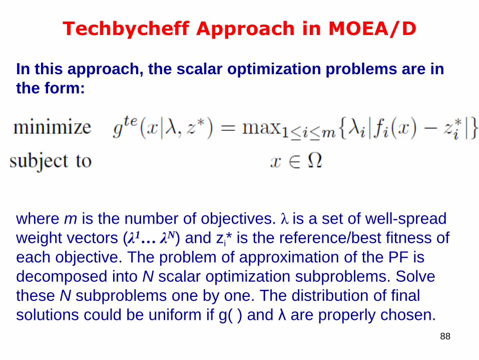
Techbycheff Approach in MOEA/D
In this approach, the scalar optimization problems are in
the form:
where m is the number of objectives. λ is a set of well-spread
weight vectors (λ1… λN) and zi* is the reference/best fitness of
each objective. The problem of approximation of the PF is
decomposed into N scalar optimization subproblems. Solve
these N subproblems one by one. The distribution of final
solutions could be uniform if g( ) and λ are properly chosen.
88
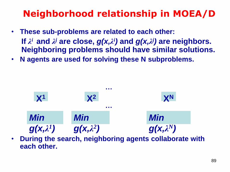
Neighborhood relationship in MOEA/D
• These sub-problems are related to each other:
If λi and λj are close, g(x,λi) and g(x,λj) are neighbors. Neighboring problems should have similar solutions.
• N agents are used for solving these N subproblems.
…
…
• During the search, neighboring agents collaborate with each other.
X1 X2 XN
Min
g(x,λ1)
Min
g(x,λ2)
Min
g(x,λN)
89
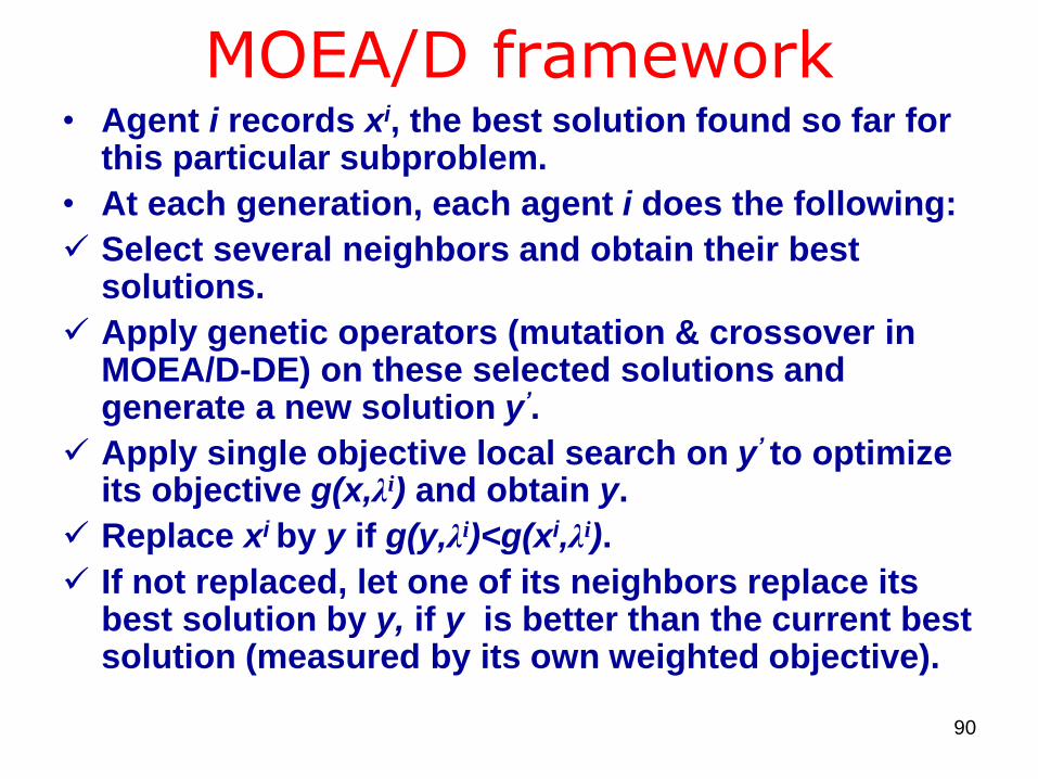
• Agent i records xi, the best solution found so far for this particular subproblem.
• At each generation, each agent i does the following:
Select several neighbors and obtain their best solutions.
Apply genetic operators (mutation & crossover in MOEA/D-DE) on these selected solutions and generate a new solution y’.
Apply single objective local search on y’ to optimize its objective g(x,λi) and obtain y.
Replace xi by y if g(y,λi)<g(xi,λi).
If not replaced, let one of its neighbors replace its best solution by y, if y is better than the current best solution (measured by its own weighted objective).
MOEA/D framework
90

• For effective performance of MOEA/D, neighborhood size
(NS) parameter has to be tuned:– A large NS promotes collaboration among dissimilar subproblems, which
advances the information exchange among the diverse subproblems, and
thus it speeds up the convergence of the whole population
– While a small NS encourages combination of similar solutions and is good
for local search in a local neighborhood, which maintains the diversity for
the whole population.
• However, in some cases, a large NS can also beneficial for
diversity recovery; while a small NS is also able to
facilitate the convergence:
– For instance, during the evolution, some subproblems may get
trapped in a locally optimal regions. In order to force those
subproblems escape from the premature convergence, a large NS
is required for the exploration.
– On the other hand, if the global optima area is already found, a
small NS will be favorable for local exploitation.
ENS-MOEA/D
91
Neighborhood sizes (NS) are a crucial control parameter in MOEA/D.
An ensemble of different neighborhood sizes (NSs) with online self-adaptation is proposed (ENS-MOEA/D) to overcome the difficulties such as
1) tuning the numerical values of NS for different problems;
2) specifications of appropriate NS over different evolution stages when solving a single problem.
S. Z. Zhao, P. N. Suganthan, Q. Zhang, "Decomposition Based Multiobjective Evolutionary Algorithm with an Ensemble of Neighborhood Sizes", IEEE Trans. on Evolutionary Computation, DOI: 10.1109/TEVC.2011.2166159, 2012.
ENS-MOEA/D
92
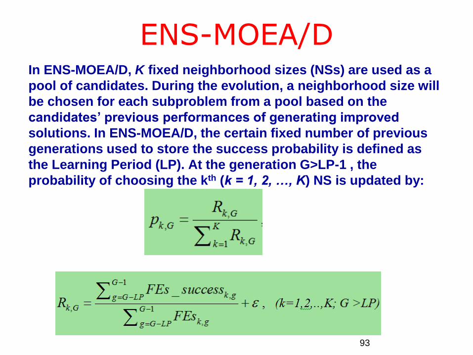
In ENS-MOEA/D, K fixed neighborhood sizes (NSs) are used as a
pool of candidates. During the evolution, a neighborhood size will
be chosen for each subproblem from a pool based on the
candidates’ previous performances of generating improved
solutions. In ENS-MOEA/D, the certain fixed number of previous
generations used to store the success probability is defined as
the Learning Period (LP). At the generation G>LP-1 , the
probability of choosing the kth (k = 1, 2, …, K) NS is updated by:
ENS-MOEA/D
93
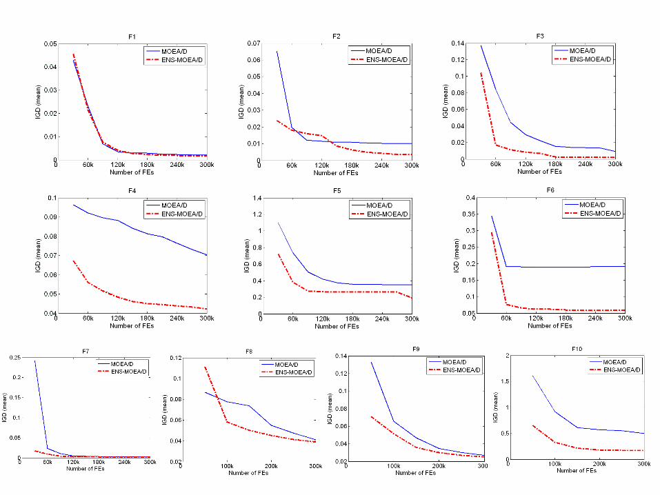
ENS-MOEA/D Experimental results
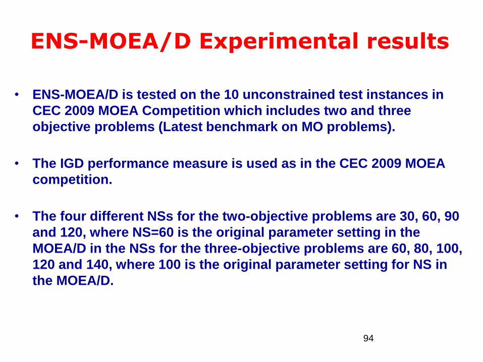
• ENS-MOEA/D is tested on the 10 unconstrained test instances in
CEC 2009 MOEA Competition which includes two and three
objective problems (Latest benchmark on MO problems).
• The IGD performance measure is used as in the CEC 2009 MOEA
competition.
• The four different NSs for the two-objective problems are 30, 60, 90
and 120, where NS=60 is the original parameter setting in the
MOEA/D in the NSs for the three-objective problems are 60, 80, 100,
120 and 140, where 100 is the original parameter setting for NS in
the MOEA/D.
94

ENS-MOEA/D Experimental results
• We conducted a parameter sensitivity investigation of LP
for ENS-MOEA/D using four different values (10, 25, 50 and
75) on the 10 benchmark instances. By observing the mean
of IGD values over 25 runs we can conclude that the LP is
not so sensitive to most of the benchmark functions, and it
is set as LP=50.
• The mean of IGD values over 25 runs among all the variants
of MOEA/D with different fixed NS and ENS-MOEA/D are
ranked. Smaller ranks, better performance.
95

96
Overview
I. Introduction to Real Variable Optimization & DE
II. Single Objective Optimization
III. Constrained Optimization
IV. Multi-objective Optimization
V. Multimodal Optimization
VI. Expensive Optimization
VII. Large Scale Optimization
VIII. Dynamic Optimization
98
Niching and Multimodal Optimization with DE
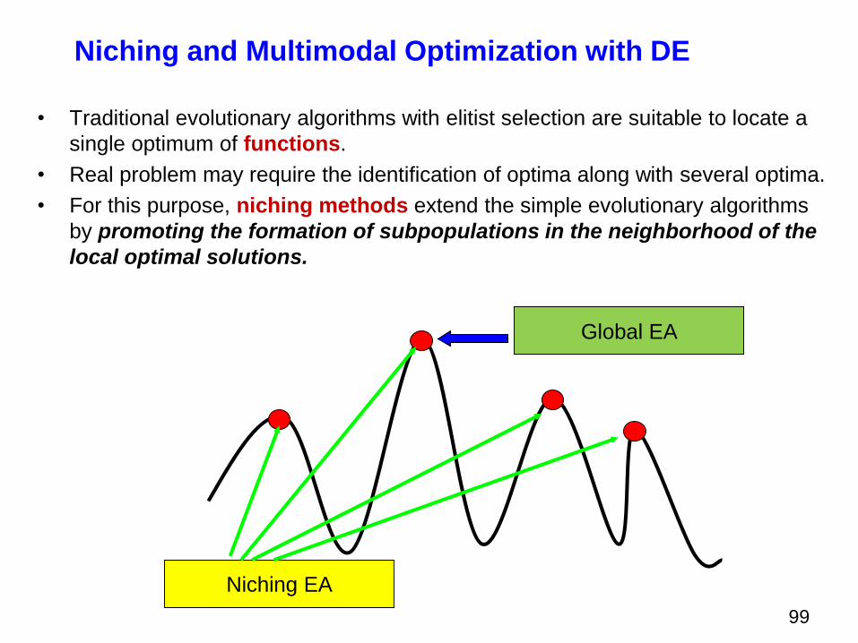
• Traditional evolutionary algorithms with elitist selection are suitable to locate a
single optimum of functions.
• Real problem may require the identification of optima along with several optima.
• For this purpose, niching methods extend the simple evolutionary algorithms
by promoting the formation of subpopulations in the neighborhood of the
local optimal solutions.
Global EA
Niching EA
99
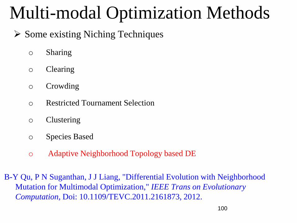
Multi-modal Optimization Methods Some existing Niching Techniques
o Sharing
o Clearing
o Crowding
o Restricted Tournament Selection
o Clustering
o Species Based
o Adaptive Neighborhood Topology based DE
100
B-Y Qu, P N Suganthan, J J Liang, "Differential Evolution with Neighborhood
Mutation for Multimodal Optimization," IEEE Trans on Evolutionary
Computation, Doi: 10.1109/TEVC.2011.2161873, 2012.

Adaptive Neighborhood Mutation Based DE
Compared with about 15 other algorithms on about 27 benchmark problems
including IEEE TEC articles published in 2010-2012 period.
B-Y Qu, P N Suganthan, J J Liang, "Differential Evolution with Neighborhood Mutation for
Multimodal Optimization," IEEE Trans on Evolutionary Computation, Doi:
10.1109/TEVC.2011.2161873, Oct. 2012. 101

Classical Speciation Technique
• Fixed speciation radius, Rspecies
• Removes population members from niches without regard for local fitness
environment
Step 1: Initialize at random a population of size N within the range of [XLower, XUpper] in D dimensions
Step 2: Compute Euclidean distance for all members
distij=√∑(xi,j)2, j=1, …D, i=1,2…N
Step 3: Sort all individuals in descending order of fitness
Step 4: Set species number S=1
WHILE sorted population is not empty
1. Identify the fittest member from sorted population and remove it as the species seed for species number S.
2. Mark all members within the speciation radius rspecies as members of the same species as S
3. Remove the speciated members from the sorted population
4. Check the number of members within species. If the specie size exceeds that of specified, remove the excess members in order of weakestfitness. On the other hand if insufficient members are in the same species, randomly initialize members within rspecies of the species seed.
5. Increment S until all members classified into species.
END WHILE
Step 5: Perform normal DE process within each species
Step 6: Repeat Steps 2 to 5 until a termination criterion

Arithmetic Recombination
Search region covered by line Arithmetic Recombination for
K= [-0.5, 0.5, 1.5]
103

Neighborhood Arithmetic Recombination-based
Speciation DE (based on DoI: . 10.1109/TCYB.2015.2394466)
• Classical niching and clustering methods highly sensitive to
parameter settings and initial population distribution in addition
to niche size
– e.g Speciation radius Rspecies, Fitness-sharing radius Rsharing, Crowding factor, CF
• Difficult to separate the initial population into niches in uneven
and rugged regions,
– i.e when niching radius contains more than one peak.
• A guaranteed way to identify separate niches: detecting fitness
valleys and peaks
• Arithmetic Recombination interpolates and extrapolates between
neighbors from niche centers (local fittest member)
• Self-adaptive generalization across different fitness terrains
• Reduction of multiple niching parameters to only neighborhood
popln size, m 104

Interpolating and Extrapolating members using
Arithmetic Recombination
X – popln member ; Star: solutions generated Arith. Recomb.
Neighborhood Arithmetic
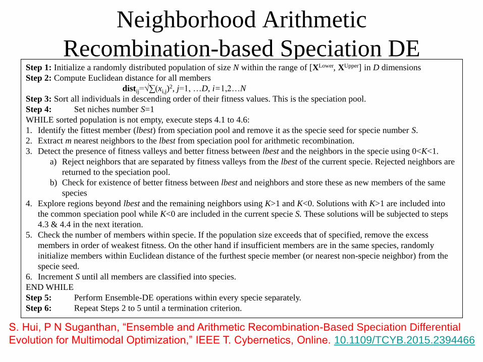
Recombination-based Speciation DEStep 1: Initialize a randomly distributed population of size N within the range of [XLower, XUpper] in D dimensions
Step 2: Compute Euclidean distance for all members
distij=√∑(xi,j)2, j=1, …D, i=1,2…N
Step 3: Sort all individuals in descending order of their fitness values. This is the speciation pool.
Step 4: Set niches number S=1
WHILE sorted population is not empty, execute steps 4.1 to 4.6:
1. Identify the fittest member (lbest) from speciation pool and remove it as the specie seed for specie number S.
2. Extract m nearest neighbors to the lbest from speciation pool for arithmetic recombination.
3. Detect the presence of fitness valleys and better fitness between lbest and the neighbors in the specie using 0<K<1.
a) Reject neighbors that are separated by fitness valleys from the lbest of the current specie. Rejected neighbors are
returned to the speciation pool.
b) Check for existence of better fitness between lbest and neighbors and store these as new members of the same
species
4. Explore regions beyond lbest and the remaining neighbors using K>1 and K<0. Solutions with K>1 are included into
the common speciation pool while K<0 are included in the current specie S. These solutions will be subjected to steps
4.3 & 4.4 in the next iteration.
5. Check the number of members within specie. If the population size exceeds that of specified, remove the excess
members in order of weakest fitness. On the other hand if insufficient members are in the same species, randomly
initialize members within Euclidean distance of the furthest specie member (or nearest non-specie neighbor) from the
specie seed.
6. Increment S until all members are classified into species.
END WHILE
Step 5: Perform Ensemble-DE operations within every specie separately.
Step 6: Repeat Steps 2 to 5 until a termination criterion.
S. Hui, P N Suganthan, “Ensemble and Arithmetic Recombination-Based Speciation Differential
Evolution for Multimodal Optimization,” IEEE T. Cybernetics, Online. 10.1109/TCYB.2015.2394466

Ensemble Parameters of EARSDE• Neighborhood size, m = 6
• Scaling factor Fi [0.3, 0.5, 0.9].
• Crossover probability Ci [0.1, 0.5].
• Binomial Crossover
• Mutation Strategies
1. DE/rand/1
viG = xrand1,i
G + F(xrand2,iG – xrand3,i
G)
2. DE/ best/1
viG = xbest
G + F(xrand1,iG – xrand2,i
G)
• Arithmetic Recombination scaling factor,
K = [-0.5, 0.5, 1.5] with additive variable, ±∆
• ∆ ϵ [0, 0.1] 107

Speciation process in EARSDE in 2D Vincent problem
• Initial population - ‘X’, initial pop-size = 60, neighborhood size = 6
• Fittest regions are represented by the darkest contours.
• Fittest member is first selected as the species seed for AR operations 108

Speciation process in EARSDE in 2D Vincent problem
• species seed is highlighted with a red square ‘□‘
• 5 nearest neighbors are highlighted with red circle ‘o’
• AR (K=0.5) applied to check for any fitness valleys.
• Midpoints represented with red plus signs ‘+’
New peak
discovered
109

Speciation process in EARSDE in 2D Vincent problem
• Existing neighbors of the species seed could not be grouped into the same species due to
fitness valleys or doubled peaks
• Random initialization executed around original species seed within 0.5 of the distance to
the nearest neighbor separated by fitness valley.
• New random members are represented by the red circles ‘●‘
Randomly initialized
species members
Newly peaks survive to
evolve in next iteration
110

Speciation process in EARSDE in 2D Vincent problem
• A neighbor rejected by the previous species now selected for speciation. Repeat process
• Dotted black lines to indicate association to species
New peak
discovered Next species
seed
111

Speciation process in EARSDE in 2D Vincent problem
• New peaks (highlighted by a red square ‘□‘ with red plus signs ‘+’) would only
enter speciation process in the next iteration
• Random members populated around new peaks.
Next species
seed
112

Overview
I. Introduction to Real Variable Optimization & DE
II. Single Objective Optimization
III. Constrained Optimization
IV. Multi-objective Optimization
V. Multimodal Optimization
VI. Expensive Optimization
VII. Large Scale Optimization
VIII. Dynamic Optimization
11
3

Expensive Optimization
• When the computation of objective value once takes
very long time, the problem is classified as expensive
optimization. In this case:
– Only a few hundreds of objective function evaluations can be
possible.
– A common approach is to develop a computationally cheap
surrogate model for the expensive objective function.
– We can make use of the surrogate model to suggest locations
in the parameter space to perform the actual objective function
computation.
– Every time a true objective value is computed, the surrogate
model can be updated.
114

Overview
I. Introduction to Real Variable Optimization & DE
II. Single Objective Optimization
III. Constrained Optimization
IV. Multi-objective Optimization
V. Multimodal Optimization
VI. Expensive Optimization
VII. Large Scale Optimization
VIII. Dynamic Optimization
11
5
Large Scale Optimization
• Optimization algorithms perform differently when
solving different optimization problems due to their
distinct characteristics. Most optimization algorithms
lose their efficacy when solving high dimensional
problems. Two main difficulties are:
– The high demand on exploration capabilities of the
optimization methods. When the solution space of a problem
increases exponentially with increasing dimensions, more
efficient search strategies are required to explore all promising
regions within a given time budget.
– The complexity of a problem characteristics may increase with
increasing dimensionality, e.g. unimodality in lower
dimensions may become multi-modality in higher dimensions
for some problems (e.g. Rosenbrock’s)
116

Large Scale Optimization
• Due to these reasons, a successful search
strategy in lower dimensions may no longer be
capable of finding good solutions in higher
dimension.
• Four LSO algorithms based on DE with the best
performances – MOS, jDElscop, SaDE-MMTS and
mDE-bES
• From the special issue of the Soft Computing
Journal on Scalability of Evolutionary Algorithms
and other Meta-heuristics for Large Scale
Continuous Optimization Problems.
117

SaDE-MMTS – Two levels of self-adaptation
SaDE benefits from the self-adaptation of trial vector generation
strategies and control parameter adaptation schemes by learning
from their previous experiences to suit different characteristic of the
problems and different search requirements of evolution phases.
Every generation, a selection among the JADE mutation strategy
with two basic crossover operators (binomial crossover and
exponential crossover) as well as no crossover option is also
adaptively determined for each DE population member based on the
previous search experiences.
S. Z. Zhao, P. N. Suganthan, and S. Das, “Self-adaptive differential evolution
with multi-trajectory search for large scale optimization”, Soft Computing,
15, pp. 2175-2185, 2011.118

SaDE-MMTS – Two levels of self-adaptation
Low Level Self-adaptation in MMTS:
An adaptation approach is proposed to adaptively
determine the initial step size parameter used in the
MMTS. In each MMTS phase, the average of all
mutual dimension-wise distances between current
population members (AveDis) is calculated, one of
the five linearly reducing factors (LRF) from 1 to 0.1,
5 to 0.1, 10 to 0.1, 20 to 0.1 and 40 to 0.1 is selected
based on the performance, and this LRF is applied
to scale AveDis over the evolution.
119
SaDE-MMTS
High Level Self-adaptation between SaDE & MMTS:
The MMTS is used periodically for a certain
number of function evaluations along with SaDE,
which is determined by an adaptive manner.
At the beginning of optimization procedure, the
SaDE and the MMTS are firstly conducted
sequentially within one search cycle by using the
same number of function evaluations. Then the
success rates of both SaDE and MMTS are
calculated. Subsequently, function evaluations are
assigned to SaDE and MMTS in each search cycle
proportional to the success rates of both search
methods.120

Experiments Results
• Algorithms were tested on 19 benchmark functions
prepared for a Special Issue on Scalability of
Evolutionary Algorithms and other Metaheuristics
for Large Scale Continuous Optimization Problems.
(http://sci2s.ugr.es/eamhco/CFP.php)
• The benchmark functions are scalable. The
dimensions of functions were 50, 100, 200, 500, and
1000, respectively, and 25 runs of an algorithm were
needed for each function.
• The optimal solution results, f (x*), were known for
all benchmark functions.
121

mDE-bES
• We boost the population diversity while preserving
simplicity by introducing a multi-population DE to solve
large-scale global optimization problems
– the population is divided into independent subgroups, each with
different mutation and update strategies
– A novel mutation strategy that uses information from either the
best individual or a randomly selected one is used to produce
quality solutions to balance exploration and exploitation.
• Mostafa Z. Ali, Noor H. Awad, Ponnuthurai N. Suganthan “Multi-
population differential evolution with balanced ensemble of
mutation strategies for large-scale global optimization” Appl.
Soft Comput. 33: 304-327 (2015)
122

mDE-bES• At the end of each epoch, individuals between the
subgroups are exchanged to facilitate information
exchange at a slow pace.
• The only link between these subgroups is the sharing of
individuals’ experiences through the migration of
individuals at constant intervals to restore balance of the
search direction affording a higher probability of
escaping basin of attraction of locally optimal solutions.
123

Migration phase
Migration with ring topology.
Migration with custom neighborhood topology.
Migration with complete net topology (free form).
The structure for the migration has several possibilities
124
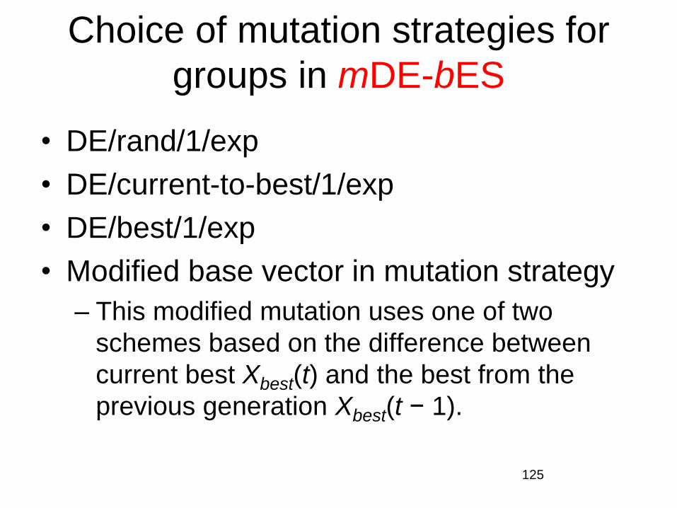
Choice of mutation strategies for
groups in mDE-bES
• DE/rand/1/exp
• DE/current-to-best/1/exp
• DE/best/1/exp
• Modified base vector in mutation strategy
– This modified mutation uses one of two
schemes based on the difference between
current best Xbest(t) and the best from the
previous generation Xbest(t − 1).
125
Experiments Results
• Algorithms were tested on 19 benchmark functions
prepared for a Special Issue on Scalability of
Evolutionary Algorithms and other Metaheuristics
for Large Scale Continuous Optimization Problems.
(http://sci2s.ugr.es/eamhco/CFP.php)
• The benchmark functions are scalable. The
dimensions of functions were 50, 100, 200, 500, and
1000, respectively, and 25 runs of an algorithm were
needed for each function.
• The optimal solution results, f(x*), were known for
all benchmark functions.
126
Overview
I. Introduction to Real Variable Optimization & DE
II. Single Objective Optimization
III. Constrained Optimization
IV. Multi-objective Optimization
V. Multimodal Optimization
VI. Expensive Optimization
VII. Large Scale Optimization
VIII. Dynamic Optimization
12
7
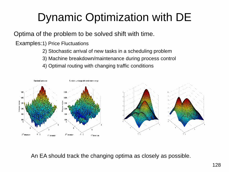
Dynamic Optimization with DE
Optima of the problem to be solved shift with time.
Examples:1) Price Fluctuations
2) Stochastic arrival of new tasks in a scheduling problem
3) Machine breakdown/maintenance during process control
4) Optimal routing with changing traffic conditions
An EA should track the changing optima as closely as possible.
128

Requirements for adopting an EA in Dynamic Environments
Boost-up diversity after an environmental change (e.g. hypermutation, variable
local search).
Maintain diversity throughout the runs with a hope that a well spread-out
population can cope with dynamic changes more easily (e.g. random immigrants,
thermodynamic GA).
Memory based approaches (particularly useful when the optimum repeatedly
returns to its previous locations).
Multi-population approach – Use of different subpopulations that can maintain
information about several promising regions of the search space – act as a
distributed and adaptive memory (e.g. multinational GAs)
Reuse of information from previous generations may help is the environmental
change is not too severe.
129
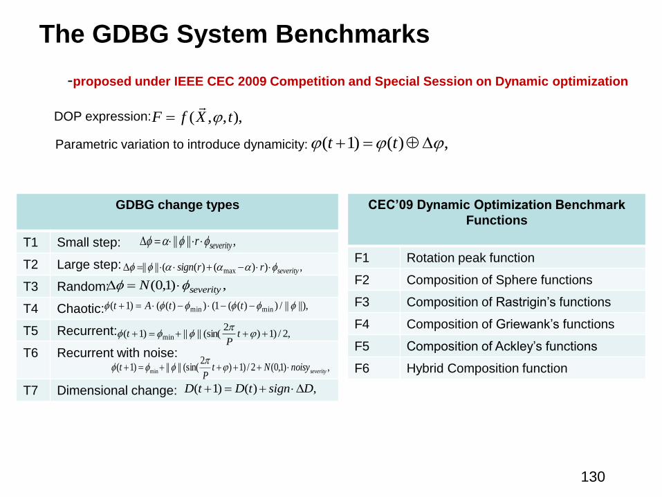
The GDBG System Benchmarks
CEC’09 Dynamic Optimization Benchmark
Functions
F1 Rotation peak function
F2 Composition of Sphere functions
F3 Composition of Rastrigin’s functions
F4 Composition of Griewank’s functions
F5 Composition of Ackley’s functions
F6 Hybrid Composition function
-proposed under IEEE CEC 2009 Competition and Special Session on Dynamic optimization
DOP expression: ( , , ),F f X t
Parametric variation to introduce dynamicity: ( 1) ( ) ,t t
GDBG change types
T1 Small step:
T2 Large step:
T3 Random:
T4 Chaotic:
T5 Recurrent:
T6 Recurrent with noise:
T7 Dimensional change:
,|||| severityr
,))()((|||| max severityrrsign
,)1,0( severityN
||),||/))((1())(()1( minmin ttAt
,2/)1)2
(sin(||||)1( min
tP
t
,)1,0(2/)1)2
(sin(||||)1( min severitynoisyNtP
t
( 1) ( ) ,D t D t sign D
130

The GDBG System Benchmarks (Contd..)
(a) Example plot of Rotation Peak function (F1) (b) Example plot of Composition of Sphere functions (F2) [inverted]
(c) Example plot of Composition of
Rastrigin’s function (F3) [inverted]
(d) Example plot of Composition of
Griewank’s function (F4) [inverted]
(e) Example plot of Composition of Ackley’s
function (F5) [inverted]
(f) Example plot of Hybrid Composition
function (F6) [inverted]
131
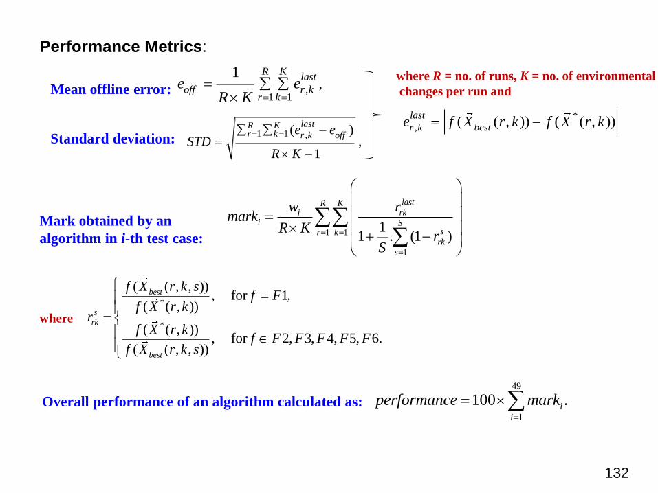
Performance Metrics:
Mean offline error: ,1 1
,1 R K
last
off r kr k
e eR K
Standard deviation:1 1 ,( )
,1
lastR Kr k r k offe e
STDR K
where R = no. of runs, K = no. of environmental
changes per run and
*
, ( ( , )) ( ( , ))last
r k beste f X r k f X r k
1 1
1
11 . (1 )
lastR Ki rk
i Ssr k
rk
s
w rmark
R Kr
S
Mark obtained by an
algorithm in i-th test case:
where
*
*
( ( , , )), for 1,
( ( , ))
( ( , )), for 2, 3, 4, 5, 6.
( ( , , ))
best
s
rk
best
f X r k sf F
f X r kr
f X r kf F F F F F
f X r k s
Overall performance of an algorithm calculated as:
49
1
100 .ii
performance mark
132

THANK YOU
Q & A
133