optimization and validation of forecasting …

176 International Journal of Current Research and Review www.ijcrr.com

Vol. 04 issue 12 June 2012

ijcrr

Vol 04 issue 12

Category: Research

Received on:12/02/12

Revised on:04/03/12

Accepted on:07/04/12

ABSTRACT Supply chain is a bridge between demand and supply. It conveys the demand to the supply point and

delivers the quantity to the demand point. It is a network, that facilities the functions of procurement of

materials, transformation of these materials into intermediate and finished products and the distribution of

these finished products to customers. The Bullwhip Effect represents the information distortion in a

Supply chain. It represents the phenomenon where orders to supplier tend to have larger variance than

sales to the buyer. The customer demand is distorted. This demand distortion also propagates to upstream

stages in an amplified form in the supply chain. The demand forecasting is one of the key-factors to

influence the bull-whip effect. Winter‘s Triple Exponential smoothening model is applied to forecast the

future demand. The purpose of this study is to analyze the impact of exponential smoothing parameters on

the bullwhip effect for Supply Chain Management (SCM). A simulation model is developed to determine

the Forecasted demand and bullwhip ratio value. Further, accuracy of Forecasting calculated by the

Winter‘s model is examined by applying Tracking Signal Technique. A sensitivity analysis is done to

experiment with the different values of parameters in the forecasting technique. It is found that longer

lead times and poor selection of forecasting model parameters lead to strong bullwhip effect in SCM. The

optimized values of parameters help to reduce the bullwhip ratio. The most significant managerial

implication of this study lies in applying best forecasting technique with accuracy testing of forecasting

model, to mitigate the bullwhip effect. The managers are suggested to utilize the best exponential

smoothing by selecting lower values for alpha and beta and a mid-value for gamma to keep the bullwhip

ratio low, besides the forecasting accuracy.

Keywords: Bullwhip ratio; Forecasting; Exponential smoothing constants; MAD; SCM; Tracking Signal

____________________________________________________________________________________

INTRODUCTION

The sources of uncertainty in a supply chain, lie

in the process of matching demand that includes

delivery lead times, manufacturing yields,

transportation times, machining times and

operator performances [10], all lead to

uncertainty in the supply chain performance.

SCM includes a set of approaches and practices

to reduce the uncertainty along the chain through

enabling a better integration among `suppliers,

manufacturers, distributors and customers [6]. It

is ‗‗the efficient management of the end-to-end

process, which starts with the design of the

product or service and ends with the time when

it has been sold, consumed, and finally,

discarded by the consumer‘‘ [12]. Demand

OPTIMIZATION AND VALIDATION OF FORECASTING

PARAMETERS TO QUANTIFY BULL-WHIP EFFECT IN A

SUPPLY CHAIN

T.V.S. Raghavendra

1, A. Rama Krishna Rao

2, P.V.Chalapathi

1

1Department of Mechanical Engineering, K.L. University, Vijayawada

2Department of Mechanical Engineering, S.V. University, Tirupati

E-mail of Corresponding Author: [email protected]



forecasting is an essential tool for production

and inventory planning, capacity management

and the design of the customer service levels.

The need to forecast the demand at each level of

the supply chain amplifies the forecast errors,

known as bullwhip effect in the supply chain. It

represents the phenomenon where orders to

supplier tend to have larger variance than sales

to the buyer, and the customer demand is

distorted [7]. This demand distortion also

propagates to upstream stages in an amplified

form. In return, high inventory levels and poor

customer service rates along the supply chain

constitute. They are the typical symptoms of

bullwhip effect. In addition, production and

inventory holding costs as well as lead times

increase, while profit margins and product

availability decrease [3][8]. In the earlier

research, the similar problem is analytically

examined by [1][2] for autoregressive demand

structures and with linear trend in the demand,

ignoring the demand seasonality.].This paper

hence presents the sensitivity analysis part &

validates forecasting accuracy using Tracking

Signal concept. Setting of experimental design is

identified, followed by simulation results.

Conclusions are in the final section. A

simulation model is developed to reduce the

bullwhip effect with forecasting parameter

optimization [9]. Tracking signal is computed by

dividing the total residuals by their mean

absolute deviation (MAD). If the tracking signal

is within 3 standard deviations, then applied

forecasting model is considered to be good

enough.

Literature survey

Uncertainty can be defined as unpredictable

events in a supply chain that affects pre-planned

performance [5]. The bullwhip effect was first

noticed and studied by [4] in a series of

simulation analysis. He named this problem as

‗‗demand amplification‘‘. It is suggested [11]

that operations managers be provided necessary

training on the bullwhip effect. However, [7]

indicates that bullwhip effect is present, even

though all members of the supply chain behave

in an optimal manner unless the supply chain is

redesigned with different strategic interactions.

Of all causes, the major emphasis has been

placed on demand forecasting. Researchers had

developed different methodologies to explore

the impact of demand forecast on bullwhip

effect. Few AR models are developed to

quantify the bullwhip effect [1] with the moving

the average forecasting model in a two-level

supply chain. Their findings support the

significance of reducing lead times to mitigate

the bullwhip effect. Under similar assumptions,

[2] also investigated the double exponential

smoothing forecasting technique for demand

process with a linear trend. [13] The impact of

forecasting parameters, demand patterns and

capacity tightness of the supplier on the

performance of the supply chain in terms of total

cost and service level is investigated by [13]. In

fact, demand forecasting has been recognized as

one of the four main causes of the bullwhip

effect [7]. As described by [9], Winter‟s triple

exponential smoothening model is used to

determine forecasted demand and the optimized

values of forecasting parameters are calculated.

The changes occurring by altering the values of

parameters in the given range is computed. The

time horizon (Year) is divided into three

seasons based on either actual demand for the

product (or) seasonality index An attempt is

made to analyze, the effect of changes in given

range of optimal values of smoothening

constants in the given season. Finally Tracking

Signal values are computed to validate

forecasting accuracy.

Model Development

The supply chain consists of four members as, a

manufacturer, a distributor, a retailer and a

consumer as shown in Fig 1.

` Fig 1 : A simple Supply Chain

An attempt is made to apply Winters‟ Triple

Exponential Model to calculate the forecasted

demand values for the given Factory,

Distributors and Retailers data. Corresponding

values of ordering quantity for Factory,

Distributors and Retailers are calculated.

The Winter‟s Triple Exponential Smoothing

Model is used to calculate the forecast demand

for Manufacturer, Distributors and Retailers.

The formula as follows

Ft+n = ( L

t + Tt x n) x S t+n-s Where n =

1,2,3…….s

Ft+n : forecast at period t+n,

Lt : level component of demand at period t,

Tt : trend component of demand at period t

S t+n-s : seasonality index for the same period the

previous year.

L t+1 = α x + (1- α) x (L t + Tt)

T t+1 = β x (Lt+1 - Lt) + (1- β) x Tt

S t+1 = γ x + (1- γ) x S t+1-s

Subject to 0 < α < 1, 0 < β < 1, 0 < γ < 1. and

α, β, γ ≥ 0.

At the beginning of each period, the retailer

receives the delivery of the distributor. Mean

while the actual customer demand emerges at

the marketplace. The retailer fulfils the customer

demand (plus back-orders if any) by on-hand

inventory, and any unfulfilled customers

demand are backordered. After the actual

customer demand is satisfied, the retailer

analyzes the historical demand data and makes a

demand forecast. The retailer decides the

quantity of items to order for the distributor

using its inventory control policy. In this case,

the manufacturer, Distributor and Retailer

follows a simple “order up to policy” to

manage the inventory. The ordering quantity is

determined by the following relation

Qt = Ft + z σt

Where Ft is forecasted demand, σt is the

standard deviation of forecasting error and z is

constant chosen to meet a desired service level.

It should be noted that z is also known as the

safety factor. Let the retailer selects a 95 % fill

rate and selects a threshold z value of 1.65.Since

the model explicitly analyzes the impact and

focuses on the role of forecasting models on the

bull-whip effect and this has a significant

diversion from the model. A similar assumption

has also been made in several studies [2].

According to [7], the bullwhip ratio is given by

the relation

Bullwhip Ratio = =

=

Subject to 0 < α < 1, 0 < β < 1, 0 < γ < 1. and α, β, γ > 0. Calculation of Tracking Signal

Manufacturer Distributor Retailer Customer



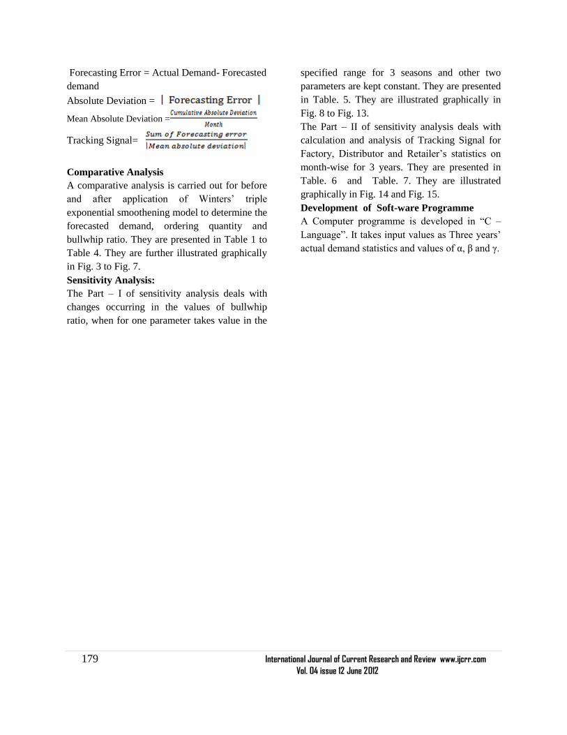
Forecasting Error = Actual Demand- Forecasted

demand

Absolute Deviation =

Mean Absolute Deviation =

Tracking Signal=

Comparative Analysis

A comparative analysis is carried out for before

and after application of Winters‘ triple

exponential smoothening model to determine the

forecasted demand, ordering quantity and

bullwhip ratio. They are presented in Table 1 to

Table 4. They are further illustrated graphically

in Fig. 3 to Fig. 7.

Sensitivity Analysis:

The Part – I of sensitivity analysis deals with

changes occurring in the values of bullwhip

ratio, when for one parameter takes value in the

specified range for 3 seasons and other two

parameters are kept constant. They are presented

in Table. 5. They are illustrated graphically in

Fig. 8 to Fig. 13.

The Part – II of sensitivity analysis deals with

calculation and analysis of Tracking Signal for

Factory, Distributor and Retailer‘s statistics on

month-wise for 3 years. They are presented in

Table. 6 and Table. 7. They are illustrated

graphically in Fig. 14 and Fig. 15.

Development of Soft-ware Programme

A Computer programme is developed in ―C –

Language‖. It takes input values as Three years‘

actual demand statistics and values of α, β and γ.



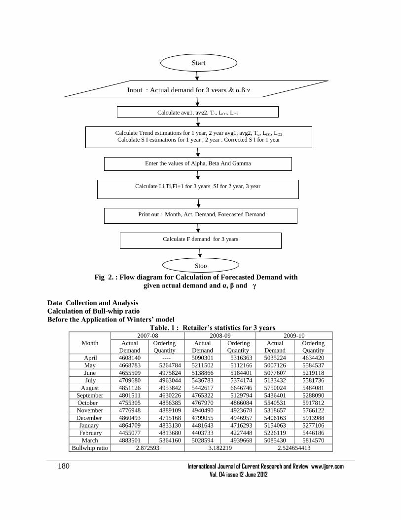
Start

Input : Actual demand for 3 years & α,β,γ

Calculate avg1, avg2, To, LO1, LO2

Calculate Trend estimations for 1 year, 2 year avg1, avg2, To, LO1, LO2

Calculate S I estimations for 1 year , 2 year . Corrected S I for 1 year

caa

Enter the values of Alpha, Beta And Gamma

Calculate Li,Ti,Fi+1 for 3 years SI for 2 year, 3 year

Calculate F demand for 3 years

Print out : Month, Act. Demand, Forecasted Demand

Stop

Fig 2. : Flow diagram for Calculation of Forecasted Demand with

given actual demand and α, β and γ

Data Collection and Analysis

Calculation of Bull-whip ratio

Before the Application of Winters‟ model

Table. 1 : Retailer‟s statistics for 3 years

Month

2007-08 2008-09 2009-10

Actual

Demand

Ordering

Quantity

Actual

Demand

Ordering

Quantity

Actual

Demand

Ordering

Quantity

April 4608140 ---- 5090301 5316363 5035224 4634420

May 4668783 5264784 5211502 5112166 5007126 5584537

June 4655509 4975824 5138866 5184401 5077607 5219118

July 4709680 4963044 5436783 5374174 5133432 5581736

August 4851126 4953842 5442617 6646746 5750024 5484081

September 4801511 4630226 4765322 5129794 5436401 5288090

October 4755305 4856385 4767970 4866084 5540531 5917812

November 4776948 4889109 4940490 4923678 5318657 5766122

December 4860493 4715168 4799055 4946957 5406163 5913988

January 4864709 4833130 4481643 4716293 5154063 5277106

February 4455077 4813680 4403733 4227448 5226119 5446186

March 4883501 5364160 5028594 4939668 5085430 5814570

Bullwhip ratio 2.872593 3.182219 2.524654413



Table. 2 : Distributor‟s statistics for 3 years

After the Application of Winters‟ model (indicated by Red color)

Table. 3 : Retailer‟s statistics for 3 years

Month

2007-08 2008-09 2009-10

Actual

Demand

Ordering

Quantity

Actual

Demand

Ordering

Quantity

Actual

Demand

Ordering

Quantity

April 4610554 ----- 5093070 4631792 5040301 4607131

May 4670604 4865308 5212546 5113716 5010000 5087902

June 4664000 4881068 5140552 5189486 5081846 5025911

July 4712513 4879484 5441404 5374961 5134995 5285036

August 4857564 4758490 5445555 6551538 5755958 5287041

September 4803735 4965763 4771889 5132830 5439241 5292872

October 4759751 4960631 4774773 4873094 5545677 5422522

November 4784000 4792097 4941774 4929204 5325311 6169536

December 4862088 4899292 4806160 4949254 5412846 5419918

January 4866237 4933242 4483586 4719638 5155369 5280683

February 4456466 4909220 4406515 4230008 5235130 4948397

March 4885850 5511160 5030453 4942506 5091294 5814570

Bullwhip Ratio 2.421206654 2.919529 3.036187691

Month

2007-08 2008-09 2009-10

Actual Demand Ordering

Quantity

Actual

Demand

Ordering

Quantity

Actual

Demand

Ordering

Quantity

April 4608140 --------- 5090301 4629078 5035224 5248684

May 4668783 4713925 5211502 5112166 5007126 5084537

June 4655509 4675824 5138866 5184401 5077607 5019118

July 4709680 4863044 5436783 5374174 5133432 5281736

August 4851126 4853842 5442617 5546746 5750024 5284081

September 4801511 4550226 4765322 5129794 5436401 5288090

October 4755305 4756385 4767970 4866084 5540531 5417812

November 4776948 4889109 4940490 4923678 5318657 5666122

December 4860493 4815168 4799055 4946957 5406163 5413988

January 4864709 4733130 4481643 4716293 5154063 5277106

February 4455077 4613680 4403733 4327448 5226119 4946186

March 4883501 5064160 5028594 4939668 5085430 5814570

Bullwhip ratio 1.248698892 0.982596542 1.275902



With the Optimized values of α = 0.76, β = 0.01, γ = 0.01

Table. 4 : Distributors‟ statistics for 3 years

Month

2007-08 2008-09 2009-10

Actual Demand Ordering

Quantity

Actual

Demand

Ordering

Quantity

Actual

Demand

Ordering

Quantity

April 4610554 -------- 5093070 4631792 5035224 5248684

May 4670604 4715308 5212546 5113716 5007126 5084537

June 4664000 4681068 5140552 5189486 5077607 5019118

July 4712513 4869484 5441404 5374961 51334325406163 5406163 5281736

August 4857564 4858490 5445555 5551538 5750024 5284081

September 4803735 4555763 4771889 5132830 5436401 5288090

October 4759751 4760631 4774773 4873094 5540531 5417812

November 4784000 4892097 4941774 4929204 5318657 5666122

December 4862088 4821292 4806160 4949254 5406163 5413988

January 4866237 4733242 4483586 4719638 5154063 5277106

February 4456466 4615220 4406515 4330008 5226119 4946186

March 4885850 5064160 5030453 4942506 5085430 5814570

Bullwhip Ratio 1.237408955 0.982596542 1.275902



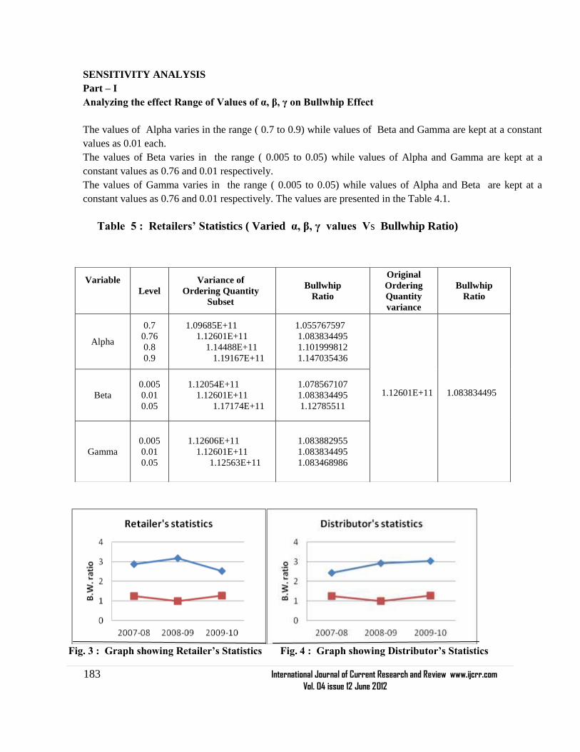
SENSITIVITY ANALYSIS

Part – I

Analyzing the effect Range of Values of α, β, γ on Bullwhip Effect

The values of Alpha varies in the range ( 0.7 to 0.9) while values of Beta and Gamma are kept at a constant

values as 0.01 each.

The values of Beta varies in the range ( 0.005 to 0.05) while values of Alpha and Gamma are kept at a

constant values as 0.76 and 0.01 respectively.

The values of Gamma varies in the range ( 0.005 to 0.05) while values of Alpha and Beta are kept at a

constant values as 0.76 and 0.01 respectively. The values are presented in the Table 4.1.

Table 5 : Retailers‟ Statistics ( Varied α, β, γ values Vs Bullwhip Ratio)

Variable

Level

Variance of

Ordering Quantity

Subset

Bullwhip

Ratio

Original

Ordering

Quantity

variance

Bullwhip

Ratio

Alpha

0.7

0.76

0.8

0.9

1.09685E+11

1.12601E+11

1.14488E+11

1.19167E+11

1.055767597

1.083834495

1.101999812

1.147035436

1.12601E+11

1.083834495

Beta

0.005

0.01

0.05

1.12054E+11

1.12601E+11

1.17174E+11

1.078567107

1.083834495

1.12785511

Gamma

0.005

0.01

0.05

1.12606E+11

1.12601E+11

1.12563E+11

1.083882955

1.083834495

1.083468986

Fig. 3 : Graph showing Retailer‟s Statistics Fig. 4 : Graph showing Distributor‟s Statistics



Fig. 5 : Alpha values with Bullwhip Ratio Fig. 6 : Beta values with Bullwhip Ratio

Fig. 7 : Gamma values with Bullwhip Ratio Fig. 8 : Gamma is 0.005 & different values of

Alpha and Beta

Fig. 9 : Gamma is 0.01 and different Fig 10 : Gamma is 0.05 and different values of

values of Alpha, Beta Alpha, Beta



Fig. 11 : Beta is 0.005 and Fig. 12 : Beta is 0.01 and for different values for

different values of Alpha and Beta of Alpha and Beta

Fig. 13 : Beta is 0.05 and for different values of Alpha and Gamma

Part – II :

Analyzing Tracking signal for both Retailer‟s and Distributor‟s statistics

The values of Tracking signal for both retailers‘ and distributors‘ data is calculated and tabulated.

The tabulated values are as shown below and analyzed to test the accuracy of forecasted model applied to

the given data.



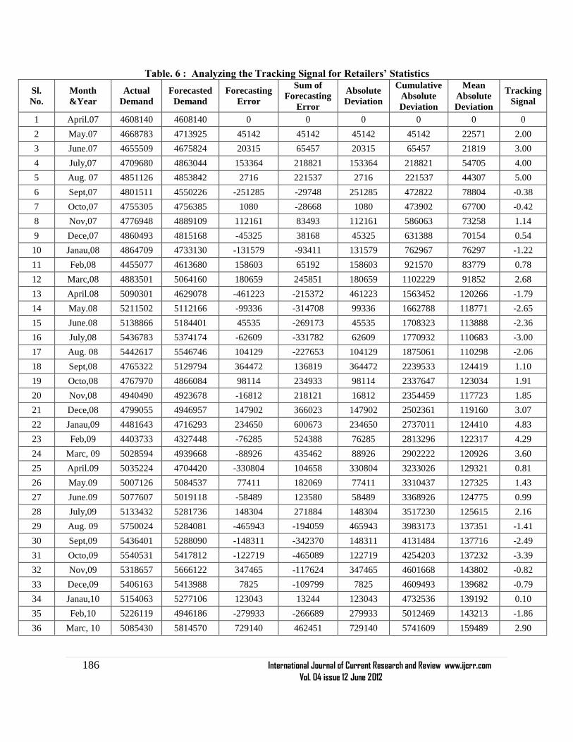
Table. 6 : Analyzing the Tracking Signal for Retailers‟ Statistics

Sl.

No.

Month

&Year

Actual

Demand

Forecasted

Demand

Forecasting

Error

Sum of

Forecasting

Error

Absolute

Deviation

Cumulative

Absolute

Deviation

Mean

Absolute

Deviation

Tracking

Signal

1 April.07 4608140 4608140 0 0 0 0 0 0

2 May.07 4668783 4713925 45142 45142 45142 45142 22571 2.00

3 June.07 4655509 4675824 20315 65457 20315 65457 21819 3.00

4 July,07 4709680 4863044 153364 218821 153364 218821 54705 4.00

5 Aug. 07 4851126 4853842 2716 221537 2716 221537 44307 5.00

6 Sept,07 4801511 4550226 -251285 -29748 251285 472822 78804 -0.38

7 Octo,07 4755305 4756385 1080 -28668 1080 473902 67700 -0.42

8 Nov,07 4776948 4889109 112161 83493 112161 586063 73258 1.14

9 Dece,07 4860493 4815168 -45325 38168 45325 631388 70154 0.54

10 Janau,08 4864709 4733130 -131579 -93411 131579 762967 76297 -1.22

11 Feb,08 4455077 4613680 158603 65192 158603 921570 83779 0.78

12 Marc,08 4883501 5064160 180659 245851 180659 1102229 91852 2.68

13 April.08 5090301 4629078 -461223 -215372 461223 1563452 120266 -1.79

14 May.08 5211502 5112166 -99336 -314708 99336 1662788 118771 -2.65

15 June.08 5138866 5184401 45535 -269173 45535 1708323 113888 -2.36

16 July,08 5436783 5374174 -62609 -331782 62609 1770932 110683 -3.00

17 Aug. 08 5442617 5546746 104129 -227653 104129 1875061 110298 -2.06

18 Sept,08 4765322 5129794 364472 136819 364472 2239533 124419 1.10

19 Octo,08 4767970 4866084 98114 234933 98114 2337647 123034 1.91

20 Nov,08 4940490 4923678 -16812 218121 16812 2354459 117723 1.85

21 Dece,08 4799055 4946957 147902 366023 147902 2502361 119160 3.07

22 Janau,09 4481643 4716293 234650 600673 234650 2737011 124410 4.83

23 Feb,09 4403733 4327448 -76285 524388 76285 2813296 122317 4.29

24 Marc, 09 5028594 4939668 -88926 435462 88926 2902222 120926 3.60

25 April.09 5035224 4704420 -330804 104658 330804 3233026 129321 0.81

26 May.09 5007126 5084537 77411 182069 77411 3310437 127325 1.43

27 June.09 5077607 5019118 -58489 123580 58489 3368926 124775 0.99

28 July,09 5133432 5281736 148304 271884 148304 3517230 125615 2.16

29 Aug. 09 5750024 5284081 -465943 -194059 465943 3983173 137351 -1.41

30 Sept,09 5436401 5288090 -148311 -342370 148311 4131484 137716 -2.49

31 Octo,09 5540531 5417812 -122719 -465089 122719 4254203 137232 -3.39

32 Nov,09 5318657 5666122 347465 -117624 347465 4601668 143802 -0.82

33 Dece,09 5406163 5413988 7825 -109799 7825 4609493 139682 -0.79

34 Janau,10 5154063 5277106 123043 13244 123043 4732536 139192 0.10

35 Feb,10 5226119 4946186 -279933 -266689 279933 5012469 143213 -1.86

36 Marc, 10 5085430 5814570 729140 462451 729140 5741609 159489 2.90



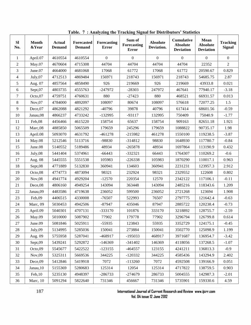
Table. 7 : Analyzing the Tracking Signal for Distributors‟ Statistics

Sl

No.

Month

&Year

Actual

Demand

Forecasted

Demand

Forecasting

Error

Sum of

Forecasting

Error

Absolute

Deviation.

Cumulative

Absolute

Deviation

Mean

Absolute

Deviation

Tracking

Signal

1 April.07 4610554 4610554 0 0 0 0 0 0

2 May.07 4670604 4715308 44704 44704 44704 44704 22352 2

3 June.07 4664000 4681068 17068 61772 17068 61772 20590.67 0.829

4 July,07 4712513 4869484 156971 218743 156971 218743 54685.75 2.87

5 Aug. 07 4857564 4858490 926 219669 926 219669 43933.8 0.021

6 Sept,07 4803735 4555763 -247972 -28303 247972 467641 77940.17 -3.18

7 Octo,07 4759751 4760631 880 -27423 880 468521 66931.57 0.013

8 Nov,07 4784000 4892097 108097 80674 108097 576618 72077.25 1.5

9 Dece,07 4862088 4821292 -40796 39878 40796 617414 68601.56 -0.59

10 Janau,08 4866237 4733242 -132995 -93117 132995 750409 75040.9 -1.77

11 Feb,08 4456466 4615220 158754 65637 158754 909163 82651.18 1.921

12 Marc,08 4885850 5065509 179659 245296 179659 1088822 90735.17 1.98

13 April.08 5093070 4631792 -461278 -215982 461278 1550100 119238.5 -3.87

14 May.08 5212546 5113716 -98830 -314812 98830 1648930 117780.7 -0.84

15 June.08 5140552 5189486 48934 -265878 48934 1697864 113190.9 0.432

16 July,08 5441404 5374961 -66443 -332321 66443 1764307 110269.2 -0.6

17 Aug. 08 5445555 5551538 105983 -226338 105983 1870290 110017.1 0.963

18 Sept,08 4771889 5132830 360941 134603 360941 2231231 123957.3 2.912

19 Octo,08 4774773 4873094 98321 232924 98321 2329552 122608 0.802

20 Nov,08 4941774 4929204 -12570 220354 12570 2342122 117106.1 -0.11

21 Dece,08 4806160 4949254 143094 363448 143094 2485216 118343.6 1.209

22 Janau,09 4483586 4719638 236052 599500 236052 2721268 123694 1.908

23 Feb,09 4406515 4330008 -76507 522993 76507 2797775 121642.4 -0.63

24 Marc, 09 5030453 4942506 -87947 435046 87947 2885722 120238.4 -0.73

25 April.09 5040301 4707131 -333170 101876 333170 3218892 128755.7 -2.59

26 May.09 5010000 5087902 77902 179778 77902 3296794 126799.8 0.614

27 June.09 5081846 5025911 -55935 123843 55935 3352729 124175.1 -0.45

28 July,09 5134995 5285036 150041 273884 150041 3502770 125098.9 1.199

29 Aug. 09 5755958 5287041 -468917 -195033 468917 3971687 136954.7 -3.42

30 Sept,09 5439241 5292872 -146369 -341402 146369 4118056 137268.5 -1.07

31 Octo,09 5545677 5422522 -123155 -464557 123155 4241211 136813.3 -0.9

32 Nov,09 5325311 5669536 344225 -120332 344225 4585436 143294.9 2.402

33 Dece,09 5412846 5419918 7072 -113260 7072 4592508 139166.9 0.051

34 Janau,10 5155369 5280683 125314 12054 125314 4717822 138759.5 0.903

35 Feb,10 5235130 4948397 -286733 -274679 286733 5004555 142987.3 -2.01

36 Marc, 10 5091294 5822640 731346 456667 731346 5735901 159330.6 4.59



Fig. 14 : Tracking signal for Retailer‟s Statistics

Fig. 15 : Tracking signal for Distributor‟s Statistics

CONCLUSIONS

The Distributor and Retailer are advised

to follow a specific Forecasting method to

estimate the future forecasting demand and

ordering quantity for next periods. Winters‘

Triple Exponential Smoothening model is

suggested.

From the study of comparative analysis,

the Bullwhip Ratio is minimum for Lower value

of Alpha, lower values of Beta and small higher

values of Gamma.

The Year is divided into Three Seasons

namely Higher, Medium and Lower. An analysis

of the relation between Bullwhip Effect with a

range of values of Alpha, Beta and Gamma with

variations of Seasonality is determined and the

following inferences are drawn.

1) During High Seasonality, to minimize the

Bullwhip Effect, the values of Alpha should be

at the lowest.


Bullwhip Effect, the values of Beta should be at

the lowest.


Bullwhip Effect, the values of Gamma should be

at the lowest.

4) During Medium Seasonality, to minimize the


at the lower value near to optimal value.



the higher value.




Bullwhip Effect, the values of Gamma should

be at the lowest value.

7) During Low Seasonality, to minimize the


at the optimal value



the optimal value.


Bullwhip Effect, the values of Gamma should

be at the higher value.

After analyzing the phenomena (pattern)

of Tracking signal for Retailer‘s Statistics, and

Distributors‘ statistics, the following inferences

are drawn.

*Tracking signal curve for Retailers‘ Statistical

data is having a range of +3.0 to - 3.0 for

many months during the 3 years of time horizon

considered, except with 2 peaks of over

estimation at July 2007 and January 2009

months, as shown in Table 6 and followed by

graph Fig 14.

*Tracking signal curve for Distributors‘

Statistical data is having a range of +4.0 to - 4.0

for many months during the 3 years of time

horizon considered, except with 1 peak of

over estimation at March 2010 month, as shown

in Table 7 and followed by the graph Fig 15.

*Hence the applied winters‘ model is found to

be more accurate.

REFERENCES

1. Chen, Y.F., Drezner, Z., Ryan, J.K., Simchi-

Levi, D., 2000a. Quantifying the bullwhip

effect in a simple supply chain: The impact

of forecasting, lead times and information.

Management Science 46, 436–443.

2. Chen, Y.F., Ryan, J.K., Simchi-Levi, D.,

2000b. The impact of exponential smoothing

forecasts on the bullwhip effect. Naval

Research Logistics 47, 269–286.

3. Chopra, S., Meindl, P., 2001. Supply Chain

Management. Prentice-Hall, Englewood

Cliffs, NJ.

4. Forrester, J., 1961. Industrial Dynamics.

MIT Press, Wiley, New York.

5. Koh, S.C.L., Gunasekaran, A., 2006. A

knowledge management approach for

managing uncertainty in manufacturing.

Industrial Management & Data Systems 106

(4), 439–459.

6. Koh, S.C.L., Demirbag, M., Bayraktar, E.,

Tatoglu, E., Zaim, S.,2007. The impact of

supply chain management practices on

performance of SMEs. Industrial

Management & Data Systems 107 (1), 103

7. Lee, H., Padmanabhan, V., Whang, S.,

1997a. The bullwhip effect in supply chains.

Sloan Management Review 38, 93–102

8. Metters, R., 1997. Quantifying the bullwhip

effect in supply chains. Journal of

Operations Management 15, 89–100.

9. T.V.S. Raghavendra, A. Ramakrishana,

P.V.Chalapathi. 2011, Quantification of

bullwhip effect with forecasting parameter

optimization in a supply chain. International

Journal of Industrial Engineering and

Technique, volume 3, Number 4, pp 427-

444.

10. Simchi-Levi, D., Kaminsky, P., Simchi-

Levi, E., 2003. Designing and Managing the

Supply Chain. McGraw-Hill, New York.

11. Sterman, J.D., 1989. Modeling managerial

behavior: Misperceptions of feedback in a

dynamic decision making experiment.

Management Science 35 (3), 321–339.

12. Swaminathan, J.M., Tayur, S.R., 2003.

Models for supply chain in E-business.

Management Science 49 (10), 1387–1406.

13. Zhao, X., Xie, J., Leung, J., 2``002. The

impact of forecasting model selection on the

value of information sharing in a supply

chain. European Journal of Operational

Research 142, 321–344.

optimization and validation of forecasting …

Documents