17a.3 numerical optimization and validation of the
TRANSCRIPT

1
Presented at the 31st AMS Conference on Hurricanes and Tropical Meteorology, San Diego, CA, 31 March – 4 April,
2014
17A.3 NUMERICAL OPTIMIZATION AND VALIDATION OF THE NEARSHORE
WAVE PREDICTION SYSTEM ACROSS THE TROPICAL ATLANTIC OCEAN DRIVEN
BY THE OFFICIAL TROPICAL ANALYSIS AND FORECAST BRANCH/NATIONAL
HURRICANE CENTER GRIDDED WIND FORECASTS
Alex Gibbs Pablo Santos NOAA/NWS/WFO Miami NOAA/NWS/WFO Miami
Miami, FL Miami, FL [email protected] [email protected]
André van der Westhuysen Roberto Padilla-Hernández IMSG at NOAA/NCEP/EMC/MMAB IMSG at NOAA/NCEP/EMC College Park, MD College Park, M [email protected] [email protected]
Hugh Cobb ` Jeffrey Lewitsky
NOAA/NWS/NHC/TAFB NOAA/NWS/NHC/TAFB Miami, FL Miami, FL
[email protected] [email protected]
Craig Mattocks NOAA/NWS/NHC/TSB
Miami, FL [email protected]
1. INTRODUCTION12
The Nearshore Wave Prediction System (NWPS, Van der Westhuysen et al. 2013) has been configured and tested across the tropical Atlantic Ocean basin through the 2013 hurricane season in experimental mode. Although this system was primarily designed to provide on-demand, high-resolution nearshore wave guidance consistent with the official forecast winds locally produced at the coastal Weather Forecast Office (WFO) across nearshore regions, further investigation through a hindcast simulation of Hurricane Isaac (2012) and daily simulations at NHC’s Tropical Analysis and Forecast Branch (TAFB) through the 2013 hurricane season have proven valuable, even for large-scale oceanic applications.
MMAB Contribution 319
This paper presents the general motivation for this development at TAFB (section 2), a description of the model setup and grid configuration across the tropical Atlantic basin (section 3) and the results of a validation period through the 2013 hurricane season (section 4). In this validation, output from NWPS and NCEP’s WAVEWATCH III
® (hereafter NWW3, Tolman
et al. 2002) model are compared against observations at various buoy stations across the Atlantic, Caribbean and Gulf of Mexico. Additionally, we discuss numerical challenges and limitations associated with official gridded wind fields generated from the NHC Tropical Cyclone Forecast Advisory Message (TCM) and the projected future adjustments necessary to further optimize the system (section 5). The conclusions of this study are provided in section 6.

2
2. MOTIVATION
The motivation for this development is two-fold: (i) to ensure consistency between the wave model guidance provided to TAFB during tropical cyclone operations and the TCM wind fields and (ii) to generate wave boundary conditions for coastal WFOs running the NWPS model in a domain residing inside the TAFB Atlantic domain. Initializing each WFO’s local wave model grid boundaries with the results from the NHC-TAFB wave model run (forced by the official NHC wind forecast) will lead to a seamless mosaic of digital marine forecasts between coastal WFOs impacted across the region, particularly during tropical cyclone events.
2.1 Consistency between waves and official
winds
The Tropical Analysis and Forecast Branch began producing gridded marine forecasts on an operational basis in April 2012. The grids are produced over their tropical North Atlantic and tropical East Pacific basins at a temporal resolution of 6 hours out to 156 hours at a spatial resolution of 10000 m. The gridded marine parameters being produced and sent experimentally to the National Digital Forecast Database (NDFD) include 10-m winds, 10-m wind gusts, and significant wave heights and hazards. During hurricane season, TAFB produces value-added 10-m wind grids utilizing the Tropical Cyclone Marine (see section 5) wind tool which creates a tropical cyclone vortex on a background wind field subject to the official forecast parameters. Tropical Storm Debby developed in the Gulf of Mexico on 23 June 2012 with advisories initiated at 2100 UTC that day. From the beginning of the storm of Mexico on 23 June 2012 with advisories initiated at 2100 UTCtilizing the Tropical Cyclone Marine ( over their tropical North Atlantic and tropical East Pacific basins at a temporal resolution of 6 hours out to ared to be a significant outlier and was forecasting a track to the northeast over Florida and off the southeast United States coast. The official NHC forecast (Figure 1) was in line with some of the better track models and the European Center for Medium-Range Weather Forecasts (ECMWF) forecast which was essentially a due west track. Forecasters at NWS forecast offices currently only have wave guidance (regional fields and boundary conditions) from NCEP’s WAVEWATCH III model (NWW3), forced by 10-m winds from either the GFS or GFDL (see below).
Figure 1: Official NHC forecast track for Tropical
Storm Debby issued at 2100 UTC 24 June 2012. Therefore they did not have access to 2D-spectra for boundary conditions which reflected the forecast wind fields from the official forecast track.
2.2 Consistency between TAFB-NHC and WFOs
TAFB was therefore in a position to provide WFOs with 2D spectral wave boundary conditions that were consistent with the official wind forecasts. The 2D-spectra derived from the official wind forecasts can be provided to the WFOs as boundary conditions for their significant wave height grids. The provision of such boundary conditions assures consistency in the wave heights between WFOs and TAFB during tropical cyclone scenarios.
3. MODEL SETUP
3.1 Computational grid
The TAFB-NWPS computational (Figure 2) grid is defined on a regular lat/lon geographical grid with a spatial grid discretization of Δx = Δy ≈ 18000 m across the tropical Atlantic and eastern Pacific basins. The grid expands northward from 3N to 32N and eastward from 98W to 10W, which is fully defined inside of the Graphical Forecast Editor (GFE) at TAFB, where the official 10000 m resolution gridded wind forecasts are created and packaged for the wave model. The spectral resolution is defined with a frequency range from 0.05 to 0.3 Hz and a directional distribution set to 36 bins (hϴ = 10
◦). Although the
official area of responsibility at TAFB extends eastward to 35W, the model grid was extended farther eastward to 10W to account for any tropical cyclone generated wave energy eastward of the area of responsibility that may approach and impact the official marine zones.
3
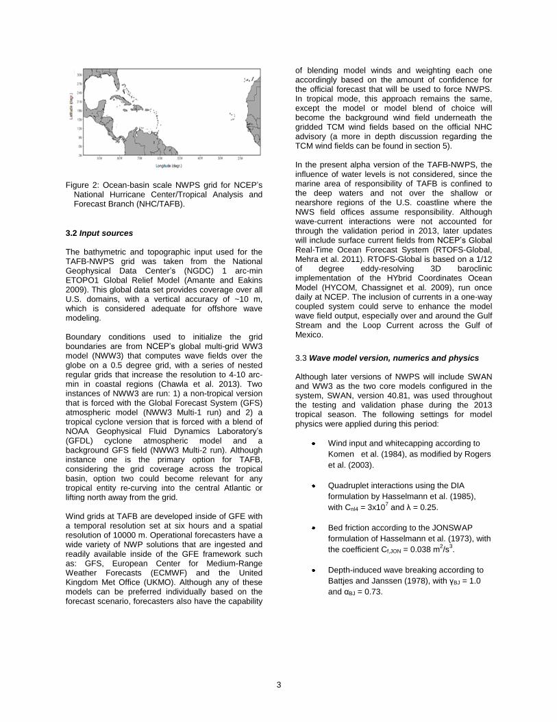
Figure 2: Ocean-basin scale NWPS grid for NCEP’s National Hurricane Center/Tropical Analysis and Forecast Branch (NHC/TAFB).
3.2 Input sources
The bathymetric and topographic input used for the TAFB-NWPS grid was taken from the National Geophysical Data Center’s (NGDC) 1 arc-min ETOPO1 Global Relief Model (Amante and Eakins 2009). This global data set provides coverage over all U.S. domains, with a vertical accuracy of ~10 m, which is considered adequate for offshore wave modeling. Boundary conditions used to initialize the grid boundaries are from NCEP’s global multi-grid WW3 model (NWW3) that computes wave fields over the globe on a 0.5 degree grid, with a series of nested regular grids that increase the resolution to 4-10 arc-min in coastal regions (Chawla et al. 2013). Two instances of NWW3 are run: 1) a non-tropical version that is forced with the Global Forecast System (GFS) atmospheric model (NWW3 Multi-1 run) and 2) a tropical cyclone version that is forced with a blend of NOAA Geophysical Fluid Dynamics Laboratory’s (GFDL) cyclone atmospheric model and a background GFS field (NWW3 Multi-2 run). Although instance one is the primary option for TAFB, considering the grid coverage across the tropical basin, option two could become relevant for any tropical entity re-curving into the central Atlantic or lifting north away from the grid. Wind grids at TAFB are developed inside of GFE with a temporal resolution set at six hours and a spatial resolution of 10000 m. Operational forecasters have a wide variety of NWP solutions that are ingested and readily available inside of the GFE framework such as: GFS, European Center for Medium-Range Weather Forecasts (ECMWF) and the United Kingdom Met Office (UKMO). Although any of these models can be preferred individually based on the forecast scenario, forecasters also have the capability
of blending model winds and weighting each one accordingly based on the amount of confidence for the official forecast that will be used to force NWPS. In tropical mode, this approach remains the same, except the model or model blend of choice will become the background wind field underneath the gridded TCM wind fields based on the official NHC advisory (a more in depth discussion regarding the TCM wind fields can be found in section 5). In the present alpha version of the TAFB-NWPS, the influence of water levels is not considered, since the marine area of responsibility of TAFB is confined to the deep waters and not over the shallow or nearshore regions of the U.S. coastline where the NWS field offices assume responsibility. Although wave-current interactions were not accounted for through the validation period in 2013, later updates will include surface current fields from NCEP’s Global Real-Time Ocean Forecast System (RTOFS-Global, Mehra et al. 2011). RTOFS-Global is based on a 1/12 of degree eddy-resolving 3D baroclinic implementation of the HYbrid Coordinates Ocean Model (HYCOM, Chassignet et al. 2009), run once daily at NCEP. The inclusion of currents in a one-way coupled system could serve to enhance the model wave field output, especially over and around the Gulf Stream and the Loop Current across the Gulf of Mexico.
3.3 Wave model version, numerics and physics
Although later versions of NWPS will include SWAN and WW3 as the two core models configured in the system, SWAN, version 40.81, was used throughout the testing and validation phase during the 2013 tropical season. The following settings for model physics were applied during this period:
Wind input and whitecapping according to
Komen et al. (1984), as modified by Rogers
et al. (2003).
Quadruplet interactions using the DIA
formulation by Hasselmann et al. (1985),
with Cnl4 = 3x10⁷ and λ = 0.25.
Bed friction according to the JONSWAP
formulation of Hasselmann et al. (1973), with
the coefficient Cf,JON = 0.038 m2/s
3.
Depth-induced wave breaking according to
Battjes and Janssen (1978), with γBJ = 1.0
and αBJ = 0.73.

4
Triad interactions using the LTA formulation
by Eldeberky (1996), with αEB = 0.05.
In addition, the following settings were applied:
• Spectral resolution was increased to include 36 directional bins (NWPS default is 24). Although this resulted in more expensive computation times, any reduction in the spectral resolution was found to result in the so-called “Garden-Sprinkler Effect”, especially as waves propagate away from tropical cyclones. Figure 3 illustrates this phenomenon for Hurricane Humberto (2013) across the central Atlantic. Due to the limited default angular resolution configured, wave energy propagates away from the storm center focusing along the directional bins in the model discretization.
• Refraction limitation: During initial runs, spurious fluctuations were found in the wave fields due to excessive refraction in regions where strong bathymetry gradients were present, mainly around small islands in the Caribbean Sea due to the large geographical grid steps. These fluctuations would begin small, then quickly radiate away from the origin leading to undesirable solutions in subsequent time steps. In order to resolve this issue, the amount of refraction over one spatial grid step had to be limited.
• Propagation time steps tested throughout the experimental period ranged between 900 and 1800 s combined with one iteration. Similar to what was illustrated in Gibbs et al. (2012), the options ranging from 900 to 1200 s proved to be the optimal solution to retain a balance between accuracy and computational time.
Figure 3: Garden-Sprinkler Effect leading to wave
energy propagating away from Hurricane Humberto (2013) focusing along the discretized directional bins in the model.
3.4 WFO boundary conditions
As mentioned above, one of the main objectives of this development was to provide the field offices with an additional source of wave guidance through wave model boundary conditions provided by TAFB. Unlike atmospheric model guidance, where forecasters are provided an abundance of NWP solutions to develop a forecast, WW3 (GFS-driven or GFDL blend during tropical cyclones) remains as the only solution for the official Coastal Waters Forecast products at the WFO level. This limitation can lead to undesirable differences across the coastal regions from site to site in an event where the NHC strongly deviates from the GFS solution, as was the case with Tropical Storm Debby (2012) discussed above. This limitation and its consequences was demonstrated by Van der Westhuysen et al., (2013) between the TAFB-NWPS and WFO New Orleans/Baton Rouge NWPS grids.
Figure 4 shows all the NWPS model domains configured at the 13 coastal WFOs in Southern Region, which are being run daily in operations. Having the option at these WFO sites to initialize the locally run wave model grid boundaries with the output of a coarser NWPS-TAFB solution (forced with the official NHC tropical cyclone advisory winds) will translate to a seamless mosaic of digital marine forecasts between coastal WFOs that are impacted in such a scenario. The same approach could be adapted year-round, even for extra-tropical applications, so that consistency is retained during high-impact marine events.

5
Figure 4: NWPS model domains (rectangles) configured at each of the 13 coastal NWS WFOs in Southern Region. Each site now has the ability to initialize the locally run NWPS grid boundaries with the TAFB-NWPS output.
3.5 Post-processing
The wave output from NWPS is post-processed into a number of model guidance products, including integral wave fields, wave spectra, and partitioned wave data. These are described below. a) Integral wave fields and wave spectra
The basic model output from NWPS are fields of the integral parameters significant wave height, peak wave period, and peak direction, typically produced every 6 h out to 102-120 h. In addition, frequency spectra are output at select locations. These outputs are all available for viewing and editing in the AWIPS II CAVE/GFE visualization module, from where it is posted to the NDFD. b) Partitioned wave fields and time series
In order to provide forecasters with a comprehensive overview of the wave systems in their region of responsibility, the directional wave spectrum at each grid point is partitioned using the inverse catchment method of Vincent and Soille (1991) and Hanson and Phillips (2001). With this method, various coherent regions of variance density in the directional spectrum are identified as separate partitions. To ensure spatial and temporal coherence, these partitioning results are consolidated into wave systems by means of spatial and temporal tracking algorithms (Van der Westhuysen et al. 2014). The resulting wave systems are presented in terms of
spatial fields and Gerling-Hanson time series plots. The latter show the progression of the wave height, period and direction of the various wave systems in time, along with the variation of local wind.
4. VALIDATION
4.1 Model evaluation period overview (2013)
An evaluation of the system across the tropical Atlantic oceanic basin was a critical step in determining whether the proposed approach would prove useful in an operational mode at this scale. Specifically, we needed to determine whether the overall behavior of the TAFB-NWPS is similar to that of the current operational guidance, namely multi-gridded tropical version of NWW3. Therefore, the results of NWPS are compared with NWW3 at various observation platforms across the region (Figure 5) from August through December 2013. To retain the highest degree of accuracy, only the initial 24 hours of the model runs were validated through the experimental period. Additionally, three tropical cyclones that developed across the region through the test period were closely evaluated and will be discussed following the test period summary at each platform where the official advisory winds (TCM winds) were used as forcing.
4.2 Model results between TAFB-NWPS and
NWW3
As previously mentioned, the official gridded wind forecast used to force NWPS at TAFB could include various combinations of techniques involving multiple model solutions between blending or even weighting certain models depending on the forecaster confidence for that period. When advisories are being issued on a tropical system, this same approach is applied, but only used as background winds to the TCM wind fields that include the official storm intensity and wind radii from the NHC advisory. For the NWW3 Multi-2, on the other hand, a blend of the GFS and GFDL 10 meter winds is applied. Figure 6 shows a linear regression analysis of the computed 10 meter winds against observations at 12 buoy platforms in the domain, for TAFB-SWAN and NWW3 Multi-2 respectively. Although both model wind sources show good correlations with the observations, the NWW3 Multi-2 (GFS/GFDL) results display a stronger correlation across all buoys than the winds used in TABF-NWPS.

6
Figure 5: NDBC buoy platforms across the Atlantic, Caribbean and Gulf of Mexico used to validate the National Hurricane Center/Tropical Analysis and Forecast Branch (NHC/TAFB) NWPS model grid from August through December of 2013.
High correlations are shown for each model source for the significant wave height (Hs), as shown in Figure 7. However, similar to the wind input driving the wave models, the NWW3 shows somewhat better correlations than TAFB-NWPS over the total validation period. The same is true at each individual station, with no significant differences or biases, even after separating the analysis into regions (Atlantic, Caribbean and Gulf of Mexico), as shown in Figures 8-10.
Figure 6: Linear regression analyses showing strong correlations between the official NHC/TAFB 10 meter forecast winds and the NWW3 Multi-2 (GFS-GFDL blend) 10 meter winds against observations at 12 buoy stations across the Atlantic, Caribbean and Gulf of Mexico.
Figure 7: Linear regression analyses showing strong to very strong correlations between the official NHC/TAFB Hs and the NWW3 Multi-2 (GFS-GFDL blend) Hs against observations at 12 buoy stations across the Atlantic, Caribbean and Gulf of Mexico.
Figure 8: Linear regression analyses at 5 buoy platforms over the deep Atlantic region all showed very strong correlations for Hs for each model source with no significant differences identified. (TAFB-NWPS (left) and NWW3 Multi-2 (right))

7
Figure 9: Linear regression analyses at 3 buoy platforms over the Caribbean region all showed very strong correlations for Hs for each model source at each station with no significant differences identified. (TAFB-NWPS (left) and NWW3 Multi-2 (right))
Figure 10: Linear regression analyses at 4 buoy platforms over the Gulf of Mexico all showed strong to very strong correlations for Hs from each model source with no significant differences identified (TAFB-NWPS (left) and NWW3 Multi-2 (right))
4.3 Tropical cyclone cases
a. Tropical Storm Chantal
Chantal developed over the tropical Atlantic, east of Barbados, on July 7, 2013 and raced westward through the Lesser Antilles to the south of Hispaniola before dissipating on July 10
th. Chantal was a small,
fast-moving system and was noted to be the fastest-moving tropical cyclone observed in the tropics within the Atlantic basin in the observational record during the satellite era (Kimberlain, 2013). Chantal reached a peak track speed of 14 to 15 ms
-1 with an estimated
peak intensity of 28 ms-1
on July 9th
while passing south of Puerto Rico and buoy station 42060 located at 16.332N and 63.240W (southeast of Puerto Rico). Figure 11 shows a combination of the best track and the 34 and 50 knot wind radii associated with Chantal while quickly passing south of buoy station 42060 on the 9
th of July. Since the 34 knot wind radii clipped the
buoy location, Chantal ended up being an excellent case to validate the official gridded TCM wind fields used to force NWPS. Similar to the seasonal validation period discussed above, forecasts were only validated out to 24 hours for each model cycle to retain accuracy. The top panel in Figure 12 shows a time series of the TCM wind magnitude, NWW3 Multi-2 (GFS/GFDL) and the GFS plotted alongside the observations from 42060. The time series is characterized with a quick peak on the 9
th of July as Chantal passed to the
south. The TCM wind magnitude ended up over-predicting the observed wind magnitude by approximately 6 ms
-1 and was around 2 to 3 ms
-1
higher than the GFS/GFDL and GFS solutions. The bottom panel of Figure 12 shows a time series of Hs, which each model seemed to converge well with the observed heights, despite the 6 ms
-1 wind magnitude
differences. These small errors between the modeled wave heights could be a result of a combination between Chantal’s small size and fast motion.
b. Hurricane Ingrid
Ingrid developed in the Bay of Campeche on September 12, 2013 and became the second and last Hurricane (Cat 1) of the 2013 hurricane season on
8
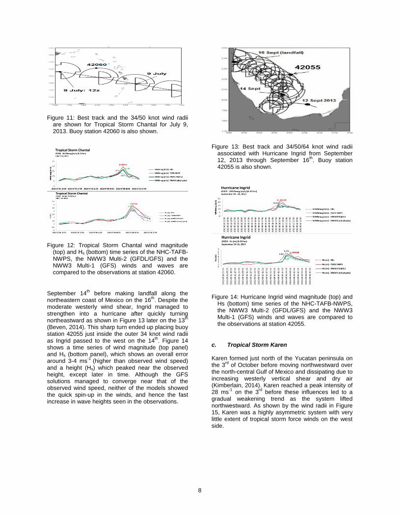
Figure 11: Best track and the 34/50 knot wind radii are shown for Tropical Storm Chantal for July 9, 2013. Buoy station 42060 is also shown.
Figure 12: Tropical Storm Chantal wind magnitude (top) and Hs (bottom) time series of the NHC-TAFB-NWPS, the NWW3 Multi-2 (GFDL/GFS) and the NWW3 Multi-1 (GFS) winds and waves are compared to the observations at station 42060.
September 14th before making landfall along the
northeastern coast of Mexico on the 16th
. Despite the moderate westerly wind shear, Ingrid managed to strengthen into a hurricane after quickly turning northeastward as shown in Figure 13 later on the 13
th
(Beven, 2014). This sharp turn ended up placing buoy station 42055 just inside the outer 34 knot wind radii as Ingrid passed to the west on the 14
th. Figure 14
shows a time series of wind magnitude (top panel) and Hs (bottom panel), which shows an overall error around 3-4 ms
-1 (higher than observed wind speed)
and a height (Hs) which peaked near the observed height, except later in time. Although the GFS solutions managed to converge near that of the observed wind speed, neither of the models showed the quick spin-up in the winds, and hence the fast increase in wave heights seen in the observations.
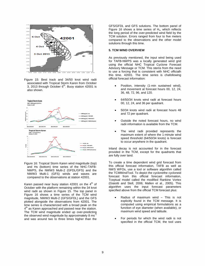
Figure 13: Best track and 34/50/64 knot wind radii associated with Hurricane Ingrid from September 12, 2013 through September 16
th. Buoy station
42055 is also shown.
Figure 14: Hurricane Ingrid wind magnitude (top) and Hs (bottom) time series of the NHC-TAFB-NWPS, the NWW3 Multi-2 (GFDL/GFS) and the NWW3 Multi-1 (GFS) winds and waves are compared to the observations at station 42055.
c. Tropical Storm Karen
Karen formed just north of the Yucatan peninsula on the 3
rd of October before moving northwestward over
the north-central Gulf of Mexico and dissipating due to increasing westerly vertical shear and dry air (Kimberlain, 2014). Karen reached a peak intensity of 28 ms
-1 on the 3
rd before these influences led to a
gradual weakening trend as the system lifted northwestward. As shown by the wind radii in Figure 15, Karen was a highly asymmetric system with very little extent of tropical storm force winds on the west side.
9
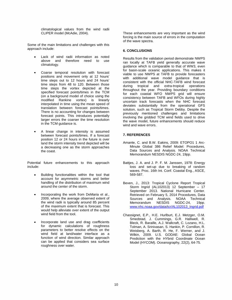
Figure 15: Best track and 34/50 knot wind radii associated with Tropical Storm Karen from October 3, 2013 through October 6
th. Buoy station 42001 is
also shown.
Figure 16: Tropical Storm Karen wind magnitude (top) and Hs (bottom) time series of the NHC-TAFB-NWPS, the NWW3 Multi-2 (GFDL/GFS) and the NWW3 Multi-1 (GFS) winds and waves are compared to the observations at station 42001.
Karen passed near buoy station 42001 on the 4th of
October with the platform remaining within the 34 knot wind radii as shown in Figure 15. The top panel in Figure 16 shows a time series of the TCM wind magnitude, NWW3 Multi-2 (GFS/GFDL) and the GFS plotted alongside the observations from 42001. The time series is characterized with a broad peak on the 4
th as Karen approached and passed near the station.
The TCM wind magnitude ended up over-predicting the observed wind magnitude by approximately 8 ms
-1
and was around two to three times higher than the
GFS/GFDL and GFS solutions. The bottom panel of Figure 16 shows a time series of Hs, which reflects the long period of the over-predicted wind field by the TCM solution. Errors ranged from four to five meters compared to the observations and the other model solutions through this time. 5. TCM WIND OVERVIEW
As previously mentioned, the input wind being used for TAFB-NWPS was a locally generated wind grid using the official NHC Tropical Cyclone Forecast Advisory Message or TCM. This stems from the need to use a forcing that is consistent with NHC officialh this time. 42001. The time series is chafollowing official forecast information:
Position, intensity (1-min sustained wind), and movement at forecast hours 00, 12, 24, 36, 48, 72, 96, and 120.
64/50/34 knots wind radii at forecast hours 00, 12, 24, and 36 per quadrant.
50/34 knots wind radii at forecast hours 48 and 72 per quadrant.
Outside the noted forecast hours, no wind radii information is available from the TCM.
The wind radii provided represents the maximum extent of where the 1-minute wind speed threshold (64/50/34 knots) is forecast to occur anywhere in the quadrant.
Inland decay is not accounted for in the forecast provided in the TCM, except for the quadrants that are fully over land. To create a time dependent wind grid forecast from this official forecast information, TAFB as well as NWS WFOs, use a tool or software algorithm called the TCMWindTool. To depict the cyclonethe cycloneid forecast from this official forecast information, Tceptual model called the modified Rankine Vortex (Giaiotti and Stell, 2006; Mallen et al., 2005). This algorithm uses the input forecast parameters specified above from the official TCM forecast plus:
Radius of maximum wind – This is not explicitly found in the TCM message. It is computed using empirical formulations as a function of eye diameter (when available), or maximum wind speed and latitude.
For periods for which the wind radii is not specified in the official TCM, the tool uses
10
climatological values from the wind radii CLIPER model (McAdie, 2004).
Some of the main limitations and challenges with this approach include:
Lack of wind radii information as noted above and therefore need to use climatology.
Coarse temporal resolution with forecast positions and movement only at 12 hours’ time steps out to 12 hours and 24 hours’ time steps from 48 to 120. Between those time steps the vortex depicted at the specified forecast points/times in the TCM (on a background model of choice using the modified Rankine vortex) is linearly interpolated in time using the mean speed of translation between forecast points/times. There is no accounting for changes between forecast points. This introduces potentially larger errors the coarser the time resolution in the TCM guidance is.
A linear change in intensity is assumed between forecast points/times. If a forecast position 12 or 24 hours in the future is over land the storm intensity trend depicted will be a decreasing one as the storm approaches the coast.
Potential future enhancements to this approach include:
Building functionalities within the tool that account for asymmetric storms and better handling of the distribution of maximum wind around the center of the storm.
Incorporating the work from DeMaria et al., 2009, where the average observed extent of the wind radii is typically around 85 percent of the maximum extent that is forecast. This would help alleviate over extent of the output wind field from the tool.
Incorporate land use and drag coefficients for dynamic calculations of roughness parameters to better resolve effects on the wind field at land/water interface as a function of wind direction. Similar approach can be applied that considers sea surface roughness over water.
These enhancements are very important as the wind forcing is the main source of errors in the computation of the wave spectra.
6. CONCLUSIONS
Results from the validation period demonstrate NWPS ran locally at TAFB yield generally accurate wave guidance which is comparable to that of WW3, even for basin-scale oceanic applications. This makes it viable to use NWPS at TAFB to provide forecasters with additional wave model guidance that is consistent with the official NHC-TAFB wind forecast during tropical and extra-tropical operations throughout the year. Providing boundary conditions for each coastal WFO NWPS grid will ensure consistency between TAFB and WFOs during highly uncertain track forecasts when the NHC forecast deviates substantially from the operational GFS solution, such as Tropical Storm Debby. Despite the previously mentioned challenges and limitations involving the gridded TCM wind fields used to drive the wave model, future enhancements should reduce wind and wave errors.
7. REFERENCES
Amante, C. and B.W. Eakins, 2009: ETOPO1 1 Arc-Minute Global 386 Relief Model: Procedures, Data Sources and Analysis. NOAA Technical Memorandum NESDIS NGDC-24, 19pp.
Battjes, J. A. and J. P. F. M. Janssen, 1978: Energy loss and set-up due to breaking of random waves. Proc. 16th Int. Conf. Coastal Eng., ASCE, 569-587.
Beven, J., 2013: Tropical Cyclone Report Tropical Storm Ingrid (AL102013) 12 September – 17 September 2013. National Hurricane Center. Retrieved on February 5, 2014 Procedures, Data Sources and Analysis. NOAA Technical Memorandum NESDIS NGDC-24, 19pp. www.nhc.noaa.gov/data/tcr/AL102013_Ingrid.pdf
Chassignet, E.P., H.E. Hurlburt, E.J. Metzger, O.M. Smedstad, J. Cummings, G.R. Halliwell, R. Bleck, R. Baraille, A.J. Wallcraft, C. Lozano, H.L. Tolman, A. Srinivasan, S. Hankin, P. Cornillon, R. Weisberg, A. Barth, R. He, F. Werner, and J. Wilkin, 2009. U.S. GODAE: Global Ocean Prediction with the HYbrid Coordinate Ocean Model (HYCOM). Oceanography, 22(2), 64-75.
11
DeMaria, M., J.A. Knaff, R. Knabb, C. Lauer, C.R.
Sampson, R.T. DeMaria, 2009: A New Method for Estimating Tropical Cyclone Wind Speed Probabilities. Weather and Forecasting. 24:6, 1573–1591.
Eldeberky, Y. (1996), Nonlinear transformations of
wave spectra in the nearshore zone, PhD thesis, Fac. of Civ. Eng., Delft Univ. of Technol., Delft, Netherlands. 203 pp. http://repository.tudelft.nl
Giaiotti, D.B. and F. Stel, 2006: The Rankine Vortex Model. University of Trieste 06: The 06: The Delft Univ. of Technol., Delft.
Gibbs, A, P. Santos, A.J. van der Westhuysen and R. Padilla, 2012. NWS Southern Region Numerical Optimization and Sensitivity Evaluation in Non-Stationary SWAN Simulations. Proceedings of the 92nd AMS Annual Meeting, New Orleans, LA.
Hanson, J.L. and O.M. Phillips, 2001. Automated Analysis of Ocean Surface Directional Wave Spectra. J. Atmos. and Ocean Tech., Vol. 18, 277-293.
Hasselmann, K., T. P. Barnett, E. Bouws, H. Carlson, D.E. Cartwright, K. Enke, J.A. Ewing, H. Gienapp, D.E. Hasselmann, P. Kruseman, A. Meerburg, P. Mueller, D.J. Olbers, K. Richter, W. Sell and H. Walden, 1973: Measurements of wind-wave growth and swell decay during the Joint North Sea Wave Project (JONSWAP). Ergaenzungsheft zur Deutschen Hydrographischen Zeitschrift, Reihe A(8), 12, 95 pp.
Hasselmann, S. and K. Hasselmann, 1985: Computations and parameterizations of the nonlinear energy transfer in a gravity-wave spectrum, Part I: A new method for efficient
computations of the exact nonlinear transfer integral. J. Phys. Oceanogr., 15, 1369-1377.
Kimberlain, T., 2013. Tropical Cyclone Report Tropical Storm Chantal (AL032013) 7 July – 10 July 2013. National Hurricane Center. Retrieved on October 8, 2013, from www.nhc.noaa.gov/data/tcr/AL032013_Chantal.pdf
Kimberlain, T., 2013. Tropical Cyclone Report Tropical Storm Karen (AL122013) 3 October – 6 October 2013. National Hurricane Center.
Retrieved on January 8, 2014, from www.nhc.noaa.gov/data/tcr/AL122013_Karen.pdf
Komen, G.J., S. Hasselmann and K. Hasselmann, 1984: On the existence of a fully-developed wind-sea spectrum. J. of Phys. Oceanogr. 14, 1271-1285.
Mallen, K.J., M. T. Montgomery, and B. Wang, 2005: Re-examining the near-core radial structure of the tropical cyclone primary circulation: Implications for vortex resiliency. J. Atmos. Sci., 62, 408-425.
McAdie, Colin J, 2004: Development of a wind radii
CLIPER model: https://ams.confex.com/ams/pdfpapers/75190.pdf
Mehra, A. I. Rivin, H.L. Tolman, T. Spindler and B. Balasubramaniyan, 2011. A Real Time Operational Global Ocean Forecast System (Poster). GODAE OceanView - GSOP - CLIVAR Workshop on Observing System Evaluation and Intercomparisons, Univ. of California Santa Cruz, CA, USA, 13-17 June.
Rogers, W.E., P.A. Wang and D.W. Wang, 2003: Investigation of wave growth and decay in the SWAN model: Three regional scale applications. J. Phys. Oceanogr., 33, 366-389.
Tolman, H. L., B. Balasubramaniyan, L. D. Burroughs, D. V. Chalikov, Y. Y. Chao, H. S. Chen, and V. M. Gerald, 2002. Development and implementation of wind generated ocean surface wave models at NCEP. Weather and Forecasting, 17, 311-333.
Van der Westhuysen, A.J., R. Padilla, P. Santos, A. Gibbs, D. Gaer, T. Nicolini, S. Tjaden, E.-M. Devaliere, H.L. Tolman, 2013: Development and validation of the Nearshore Wave Prediction System. Proc. 93rd AMS Annual Meeting, Austin, TX.
Van der Westhuysen, A.J and J.L. Hanson, 2013. Spatial and temporal tracking of wave fields from ocean basin scales to coastal waters. J. Atmos. and Ocean Tech., submitted.
Vincent, L. and P. Soille, 1991: Watersheds in digital spaces: An efficient algorithm based on immersion simulations. IEEE Transactions of Pattern Analysis and Machine Intelligence, 13, 583–598.

12
8. ACKNOWLEDGEMENTS
The authors acknowledge the contribution and support provided by the ITO staff at NHC/TAFB regarding the hardware or platform necessary to run the system through this experimental test phase.