www.CalSolarResearch.ca.gov

Final Subtask 2 Project Report:

Mitigation of Fast Solar Ramps

through Improving Sky Imager

Solar Forecasting through

Cloud Base Height

Optimization

Grantee:

University of California

San Diego

July 2015

California Solar Initiative

Research, Development, Demonstration

and Deployment Program RD&D:

PREPARED BY

Principal Investigator: Jan Kleissl 858-534-8087 Dept of Mechanical & Aerospace Engineering Center for Renewable Resources & Integration and the Center for Energy Research

9500 Gilman Drive La Jolla, CA 92093-0411

Project Partners: San Diego Gas & Electric

PREPARED FOR

California Public Utilities Commission California Solar Initiative: Research, Development, Demonstration, and Deployment Program

CSI RD&D PROGRAM MANAGER

Program Manager: Smita Gupta Smita.Gupta@itron.com

Project Manager: Smita Gupta Smita.Gupta@itron.com

Additional information and links to project related documents can be found at http://www.calsolarresearch.ca.gov/Funded-Projects/

DISCLAIMER

“Any opinions, findings, and conclusions or recommendations expressed in this material are those of the author(s) and do not necessarily reflect the views of the CPUC, Itron, Inc. or the CSI RD&D Program.”

Preface

The goal of the California Solar Initiative (CSI) Research, Development, Demonstration, and Deployment (RD&D) Program is to foster a sustainable and self-supporting customer-sited solar market. To achieve this, the California Legislature authorized the California Public Utilities Commission (CPUC) to allocate $50 million of the CSI budget to an RD&D program. Strategically, the RD&D program seeks to leverage cost-sharing funds from other state, federal and private research entities, and targets activities across these four stages:

Grid integration, storage, and metering: 50-65%

Production technologies: 10-25%

Business development and deployment: 10-20%

Integration of energy efficiency, demand response, and storage with photovoltaics (PV)

There are seven key principles that guide the CSI RD&D Program:

1. Improve the economics of solar technologies by reducing technology costs and increasing system performance;

2. Focus on issues that directly benefit California, and that may not be funded by others;

3. Fill knowledge gaps to enable successful, wide-scale deployment of solar distributed generation technologies;

4. Overcome significant barriers to technology adoption;

5. Take advantage of California’s wealth of data from past, current, and future installations to fulfill the above;

6. Provide bridge funding to help promising solar technologies transition from a pre-commercial state to full commercial viability; and

7. Support efforts to address the integration of distributed solar power into the grid in order to maximize its value to California ratepayers.

For more information about the CSI RD&D Program, please visit the program web site at www.calsolarresearch.ca.gov.

2

Abstract Cloud base height (CBH) is a critical input to short-term solar forecasting algorithms, yet CBH measurements are difficult to obtain. We describe the integration of a cloud shadow speed sensor (CSS) with a sky imager to geolocate clouds by determining their CBH. The CSS measured cloud motion vectors at the UC San Diego campus over two months, which are compared to cloud pixel speed from the sky imagers to estimate local CBH. The CBH estimate is validated against measurements from METAR and an on-site ceilometer. Specific examples of CBH results are presented and a summary of CBH error metrics is tabulated. Typical daily root mean square differences are 160 m which corresponds to 17.42% when divided by the observed CBH. The largest nRMSD remains below 30% for all the days. However, the daily bias usually being less than 80 m suggests that the method is robust and that most of the RMSD is driven by short-term random fluctuations in CBH.

Nomenclature 𝐂𝐁𝐇 Cloud base height 𝑪𝑺𝑺 Cloud Speed Sensor

𝜽𝒎 Field of view of the USI in degrees from the vertical

𝑪𝑩𝑯𝑪𝑺𝑺+𝑼𝑺𝑰 Local CBH derived from CSS measurements and USI cloud pixel speed

𝑫 Radius of the CSS sensor circle ∆𝒕𝒊𝒋 Time shift of cloud arrival time between CSS sensors 𝒊 and 𝒋

𝑪𝑩𝑯𝒄𝒆𝒊𝒍𝒐

CBH estimates from the ceilometer

𝜽𝒔𝒆𝒏𝒔𝒐𝒓 Angle offset between sensors on the CSS

𝒏 Number of pixels of cloud map

MCP Most Correlated Pair method for cloud speed measurement

𝑹𝒊𝒋 Maximum cross-correlation coefficient of sensor pair 𝒊 - 𝒋

𝑼𝑼𝑺𝑰 USI derived cloud speed in pixel s-1

𝑼𝑪𝑺𝑺 CSS cloud speed in m s-1 𝑼𝒑𝒊𝒙𝒆𝒍 Cloud pixel speed

𝐑𝐌𝐒𝐃 Root mean square difference 𝐧𝐑𝐌𝐒𝐃 Normalized root mean square difference

AGL Above ground level MSL Mean sea level

CMV Cloud motion vector N Total number of data points

USI UC San Diego Sky Imager

1. Introduction

Short-term solar forecasting has become an important need in the solar industry. In solar forecasting, ramp rate estimation is critical because the sudden shortage or oversupply in solar power must be compensated for with an opposing ramp from energy storage or conventional generation. Cloud base height (CBH) is a major source of forecast error during short-term solar forecasting. Incorrect CBH leads to an offset between the vertical projection of a cloud onto the ground and the actual shadow location. In addition, inaccurate cloud speed associated with CBH

3

errors causes errors in the estimates of arrival time of cloud shadows, which leads to offsets in ramp timing.

Existing methods to detect CBH includes radiosondes and ceilometers. A radiosonde is a battery-powered telemetry instrument package that vertically profiles the atmosphere. Although the measurement is accurate as it is taken in-situ, the observations are usually taken only twice daily at major airports. The frequency is insufficient for intra-hour forecasting. Ceilometers, as the most common CBH observational tool, emit a high intensity near-infrared laser beam vertically. Then a vertical profile of atmospheric backscatter is obtained and CBH can be computed with sub-minute resolution. Ceilometer CBH measurements are usually reported in meteorological aerodrome reports (METAR). While METAR stations report high quality CBH data, limited temporal resolution (hourly reports) and spatial variability in cloud coverage and CBH, especially in coastal environments, causes differences between METAR and local CBH. Since the cost of ceilometers is relatively high, their application outside of airports is limited. The cloud speed sensor (CSS) offers an alternative to direct CBH measurements when combined with a sky imager. Since the cloud pixel speed (or angular cloud speed) determined by the sky imager can be expressed as the ratio of cloud speed [m s-1] and CBH, CBH can be computed from collocated sky imager and CSS measurements. This paper is organized in five sections. The UCSD CSS and data availability will be described in Section 2. The previous and new algorithm to derive cloud speed from CSS raw data are described in Sections 3.1 and 3.2. Sections 3.3 and 3.4 introduce the algorithm to determine CBH from sky imager and CSS measurements. Section 4 provides validation against an on-site ceilometer. Section 5 provides conclusions on the method, applications, and future work.

2. Hardware 2.1 Cloud Speed Sensor (CSS) The CSS (Fung et al. 2014) is a compact and economical system that measures cloud shadow motion vectors (CMVs). The system consists of an array of eight satellite phototransistors (TEPT4400, Vishay Intertechnology Inc., USA) positioned around a phototransistors located at the center of half circle of radius 0.297 m, covering 0-105° in 15° increments (Fig. 1). The sensors have a spectral response ranging from approximately 350 to 1000 nm with peak sensitivity at 570 nm. Sensor response time was determined experimentally in a laboratory controlled environment and was found to be 21 μs rise time (10-90% response). High-frequency irradiance data are taken from all sensors and fed to a high-performance 32 bit microcontroller (chipKIT Max32, Digilent Inc., USA). The on-board static memory allows fast storage of up to 6,000 10 bit data points per sensor corresponding to 9 sec of data at a time. These 9 sec of data are then processed to determine CMVs as described in Section 3.

4

Figure 1: Cloud shadow Speed Sensor (CSS) contained inside a weather proof enclosure with dimensions 0.45 x 0.40 m. On the top of the enclosure is an array of nine phototransistors.

The CMVs used in this analysis were taken from a CSS located at 32.8810°N, -117.2328°W, 106 m above mean sea level (MSL) (marked as CSS in Figure 2) and the sky images were taken by a UCSD Sky Imager (USI) located at 32.8722°N, -117.2409°W, 129 m MSL (marked as USI1_2 in Figure 2). Measurements of CBH were taken by a Vaisala CT25K ceilometer co-located with the CSS. While the sensors report CBH above ground level (AGL), the elevation of the sensor was added to obtain CBH (MSL).

5

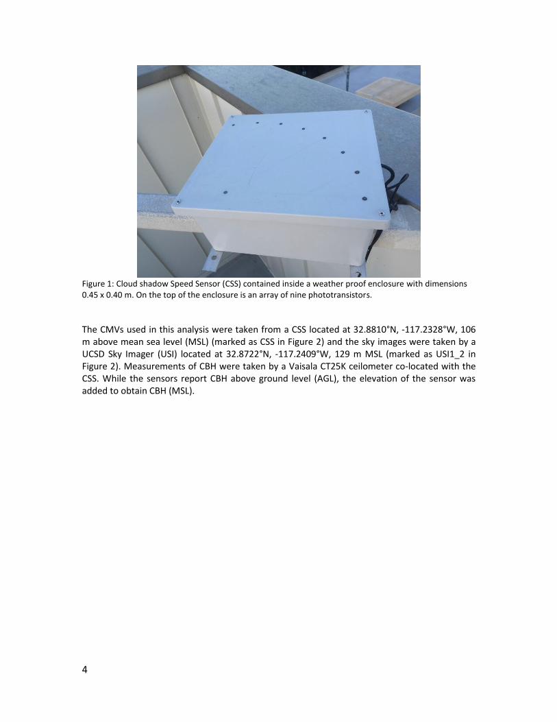
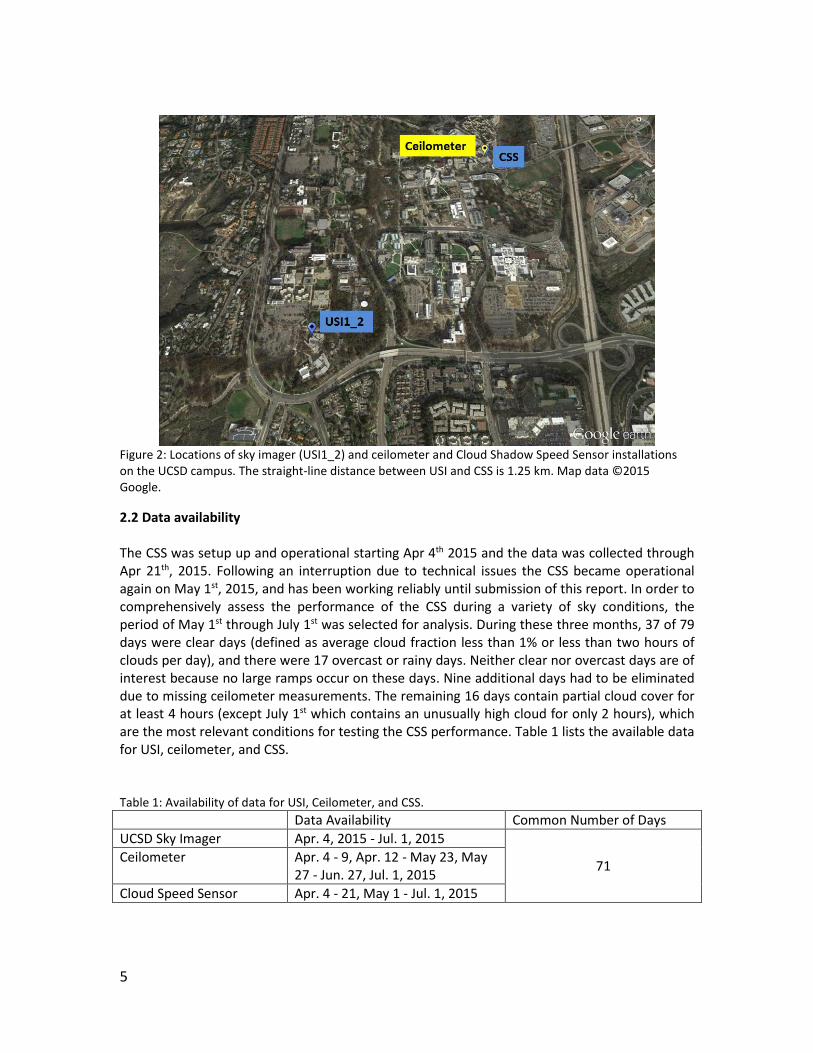
Figure 2: Locations of sky imager (USI1_2) and ceilometer and Cloud Shadow Speed Sensor installations on the UCSD campus. The straight-line distance between USI and CSS is 1.25 km. Map data ©2015 Google.

2.2 Data availability The CSS was setup up and operational starting Apr 4th 2015 and the data was collected through Apr 21th, 2015. Following an interruption due to technical issues the CSS became operational again on May 1st, 2015, and has been working reliably until submission of this report. In order to comprehensively assess the performance of the CSS during a variety of sky conditions, the period of May 1st through July 1st was selected for analysis. During these three months, 37 of 79 days were clear days (defined as average cloud fraction less than 1% or less than two hours of clouds per day), and there were 17 overcast or rainy days. Neither clear nor overcast days are of interest because no large ramps occur on these days. Nine additional days had to be eliminated due to missing ceilometer measurements. The remaining 16 days contain partial cloud cover for at least 4 hours (except July 1st which contains an unusually high cloud for only 2 hours), which are the most relevant conditions for testing the CSS performance. Table 1 lists the available data for USI, ceilometer, and CSS. Table 1: Availability of data for USI, Ceilometer, and CSS.

Data Availability Common Number of Days

UCSD Sky Imager Apr. 4, 2015 - Jul. 1, 2015

71 Ceilometer Apr. 4 - 9, Apr. 12 - May 23, May

27 - Jun. 27, Jul. 1, 2015

Cloud Speed Sensor Apr. 4 - 21, May 1 - Jul. 1, 2015

6

3. Methods

3.1 Prior cloud speed sensor algorithm In the prior CSS algorithm, the CMVs were determined by the Most Correlated Pair Method (MCP). MCP assumes that due to heterogeneity in the cloud shadow over the area of the sensor, the pair of sensors that lie along the direction of cloud motion will experience the largest cross-correlation as they see the same section of the cloud (Bosch et al., 2013). The method produced accurate results, but also suffered from some deficiencies. For example, for the ideal case of a linear cloud edge separating shadow from clear sky, each sensor would see exactly the same signal shape and there is no single most correlated pair. Instead, the most correlated pair would simply result from arbitrary correlations from sensor noise. This scenario was found to be common. Since clouds are typically much larger than the spacing between sensors, it seems intuitive that the cloud is unlikely to change significantly over the area of the CSS. Thus, CMV results were highly variable. Bosch et al. (2013) addressed the variability through statistical post-processing to determine the most common cloud direction and corresponding cloud speed. The post-processing was shown to be robust and accurate, but the temporal averaging reduced the response of the sensor to instant changes in cloud velocity.

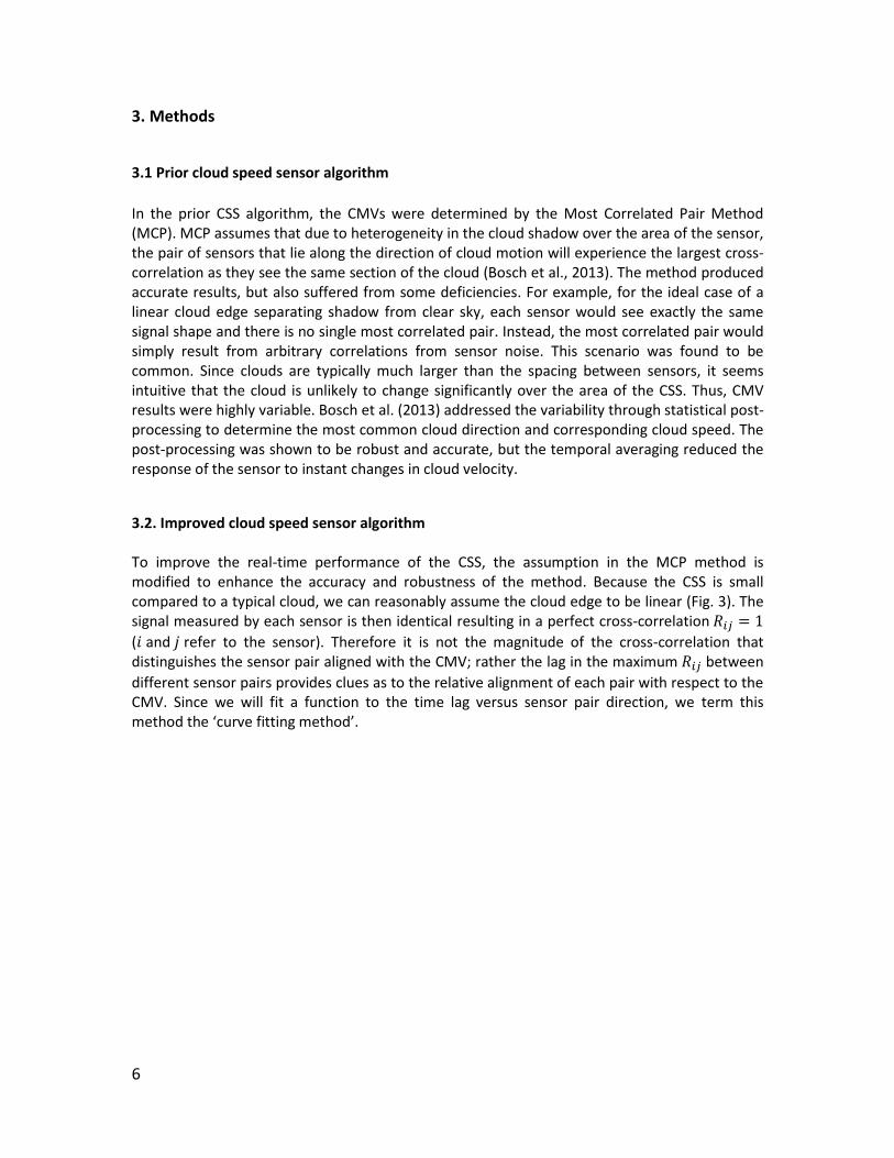
3.2. Improved cloud speed sensor algorithm To improve the real-time performance of the CSS, the assumption in the MCP method is modified to enhance the accuracy and robustness of the method. Because the CSS is small compared to a typical cloud, we can reasonably assume the cloud edge to be linear (Fig. 3). The signal measured by each sensor is then identical resulting in a perfect cross-correlation 𝑅𝑖𝑗 = 1

(𝑖 and 𝑗 refer to the sensor). Therefore it is not the magnitude of the cross-correlation that distinguishes the sensor pair aligned with the CMV; rather the lag in the maximum 𝑅𝑖𝑗 between

different sensor pairs provides clues as to the relative alignment of each pair with respect to the CMV. Since we will fit a function to the time lag versus sensor pair direction, we term this method the ‘curve fitting method’.

7

Figure 3. Illustration of the linear cloud edge assumption and curve fitting method on top of the CSS luminance sensor arrangement. Each circle represents a sensor arranged in a circular pattern with 15° radial spacing about the central sensor. Additional angles from 120° to 165° are obtained through equilateral triangles constructed from existing sensor positions. The linear cloud edge is shown as a blue line and is assumed to be advected along the line connecting sensors a and c.

As in the previous method, the maximum cross-correlation coefficient 𝑅𝑖𝑗 in each pair of signals

will be determined (Fung et al., 2014) and the associated time shift ∆𝑡𝑖𝑗 for that pair will be

recorded. To proceed, considering a linear cloud edge is crossing the CSS along the a-c sensor line, it is straightforward that:

𝐷 × 𝑐𝑜𝑠 ∅𝑠𝑒𝑛𝑠𝑜𝑟𝑖𝑗

= 𝑈𝐶𝑆𝑆 × ∆𝑡𝑖𝑗,(1)

where 𝐷 is radius of the sensor circle, ∅𝑠𝑒𝑛𝑠𝑜𝑟𝑖𝑗

is the angle between the line (a-c) and the line

connecting sensor 𝑖 and sensor 𝑗 (𝑖 and 𝑗 = 1 to 8), 𝑈𝐶𝑆𝑆 is the speed of the cloud edge, i.e. cloud speed. With distance 𝐷 and cloud speed 𝑈𝐶𝑆𝑆 constant for each pair, the time shift ∆𝑡𝑖𝑗

becomes a function of cos ∅sensor. For the ideal assumption of a linear cloud edge, plotting ∆𝑡 versus ∅ would therefore be expected to represent a cosine function. For verification, the cosine function is used to fit all ∆𝑡 versus ∅ points, and the R2 value is employed to determine the goodness of the fit (Fig. 4). A high R2 supports the linear cloud edge assumption. Since the sensor pair aligned with the cloud motion line is farthest apart (along the CMV) at a distance 𝐷, the maximum of the cosine function which represents the longest time shift ∆𝑡𝑖𝑗 should occur at the CMV direction. The

cloud velocity then becomes the ratio of the distance 𝐷 and the time shift ∆𝑡𝑖𝑗:

𝑈𝐶𝑆𝑆 =𝐷

∆𝑡𝑖𝑗. (2)

Figure 4 illustrates the procedure using 9 sec of luminance data. It is observed that correlations between all sensor pairs are very large (>0.999), which causes issues in the robustness of the

8

previously used MCP method. On the other hand, the linear cloud edge assumption is validated in that the time shift is indeed a strong function of the cosine of the direction. As a result the CMV direction and speed (using Eq. 2) can be obtained with confidence. In the example in Fig. 4 the time shift is determined as ∆𝑡 = 0.1035 s, and the corresponding direction is ∅ = 325˚ (as indicated by dotted black line) yielding a cloud speed 𝑈𝐶𝑆𝑆 = 2.87 m s-1 per Eqn. 2. Note that for data quality control, two filters are applied: If the average 𝑅𝑖𝑗 is less than 0.9 or R2

of the cosine curve fit is less than 0.9, no cloud speed will be computed. Small 𝑅𝑖𝑗 is likely a

result of no cloud passage or dynamic clouds. A small R2 indicates poor curve fitting and therefore an unreliable result. If both 𝑅𝑖𝑗 and R2 pass quality control, the extrema of the curve

fit yields the cloud direction. If ∆𝑡𝑖𝑗 of the extrema is negative, the cloud is moving in the

opposite direction compared to what is assumed in Figure 3. Then we will use the absolute value of ∆𝑡𝑖𝑗 to calculate cloud velocity and subtract 180° from ∅ of the extremum to account for the

shift in direction:

∆𝑡𝑖𝑗 = |∆𝑡𝑖𝑗|; ∅𝑜𝑝𝑝𝑜𝑠𝑖𝑡𝑒 = ∅ − 180°. (3)

Figure 4: Illustration of the curve fitting method to determine CMVs. The x-axis represents direction ∅ that is equal to (360° − i × 15°), the y-axis represents the time shift ∆𝑡𝑖𝑗 , and the color indicates the

strength of correlation 𝑅𝑖𝑗. The green curve indicates the best fit of ∆𝑡𝑖𝑗 = 0.1036 × cos (∅ + 37.26°).

The maximum time shift of the cosine function is selected as the direction of cloud motion as identified by the vertical dashed black line. Figure 5 reformats the data shown in figure 4 through a polar coordinate plot of the cloud direction ∅ versus the time shift ∆t to intuitively illustrate the choice of CMV direction. The black curve transforms the curve fit from Cartesian coordinate to polar coordinate system, while the purple arrow indicates the direction that corresponds to the maximum of the radius specified in value of time shift ∆t. Thus, the arrow vector points out the preferred CMV direction

9

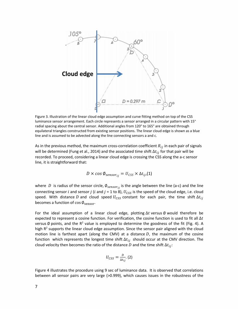
and the vector’s magnitude is the preferred time shift.

Figure 5: Illustration of the curve fitting method to determine the CMVs in polar coordinates. The concentric circles represents different time shifts ∆t and the radial lines indicate the cloud direction ∅. The red points correspond to the ∆t versus ∅ points in Figure 4. The purple arrow indicates the preferred direction of cloud motion and corresponding time shift. Figure 6 shows a set of CMVs for one day. Clouds are moving slowly at 1 to 6 m s-1 from north to south changing to easterly as the day progresses. There is some variability in the signal, but that is likely a result of both physical cloud dynamics and sensor noise. Again, we use a wind-rose plot to extend figure 6 to show the histogram of the CMVs on this days by showing the frequency of speed and direction pairs. It is noticeable that most of CMVs cluster in north-east direction with an average speed range of 2-6 m s-1.

10

Figure 6: Cloud direction and cloud speed determined by the curve fitting method on May 31th, 2015 using

9 sec segments of CSS data. The color provides the average cross correlations 𝑅𝑖𝑗 for each pair of points

during each 9 sec cycle.

Figure 7: Wind-rose plot of cloud direction and cloud speed of the data shown in Figure 6. The color bins show cloud speed range, and the values on concentric circles represent the frequency of appearance of each cloud speed bin.

11

In summary, compared to the prior MCP method, the curve fitting method yields several advantages: (i) more clustered, i.e. robust CMV results without post-filtering, and (ii) continuous cloud direction output compared to the 15-degree (equivalent to the angular arrangement of the sensors) discretized output for the MCP method. To demonstrate the improvement of the curve fitting method, an example of the prior MCP method is provided in the appendix. The disadvantage is that since the curve fitting method calculates correlation for all sensor pairs, the calculation triples the computational cost on the microcontroller to 40 sec. Therefore for this application, the processing was performed on a remote computer instead, which decreases computation time by an order of magnitude.

3.3 Cloud pixel speed from USI data

In this section, we will first introduce the USI cloud motion algorithm, and based on that in conjunction with the CSS cloud speed, a local CBH determination method will be introduced. The USI can be used to detect cloud fields and track cloud motion. These measurements yield forecast of future cloud locations at high spatial and temporal resolutions and improve forecast skill up to a 20 min forecast horizon. The benefit of using sky imager observations over a large ground sensor network is that only one or a few instruments deployed around the area of interest are capable of determining the current distribution of cloud cover at a high resolution. The forecast procedure is outlined in the flow chart in Fig. 8. The USI forecast procedure is briefly explained within this section. For more details consult Chow et al. (2011), Ghonima et al. (2012), and Yang et al. (2014).

12

Figure 8: Flowchart of the sky imager solar forecast procedure. CBH is used to project clouds onto a cartesian sky coordinate system, to obtain cloud speed, and to project the advected cloud shadows to the ground. Cloudy pixels are detected using spectral information from the RGB images. CBH is then used in conjunction with a pseudo-cartesian transform to map these clouds to a latitude-longitude grid at the cloud altitude (Chow et al., 2011). In this step, CBH is required. In absence of local data, CBH is taken from the closest meteorological aerodrome reports (METAR). The resulting georeferenced map of clouds is termed the 'cloud map', which is a planar mapping of cloud position at a specified altitude above the forecast site. Cloud pixel velocity is obtained by applying the cross-correlation method (CCM, Chow et al., 2011) to the RBR of two consecutive cloud maps. The cloud velocity [m s-1] is then calculated by converting from cloud pixel speed [pixel s-1] to cloud shadow speed using a velocity scaling factor which is a function of CBH (see Eq. 4 later). Note that since the distance from sun to earth is much larger than the distance from cloud to earth, the cloud shadow speed is essentially identical to the cloud speed.

3.4 Cloud base height determination from CSS and USI data In this section, we introduce the mathematical algorithm that constrains the CBH for sky imager forecasting with cloud speed measurements from the CSS. In the USI forecast, cloud velocity is calculated by converting from cloud pixel speed to equivalent m s-1 cloud speed as

𝑈𝑈𝑆𝐼 = 𝑈𝑝𝑖𝑥𝑒𝑙 ×𝐶𝐵𝐻×2𝑡𝑎𝑛𝜃𝑚

𝑛, (4)

where 𝑈𝑈𝑆𝐼 is cloud speed in units of m s-1 determined by USI, 𝑈𝑝𝑖𝑥𝑒𝑙 is image-average cloud

13

pixel speed in units of pixel s-1 obtained through the cross-correlation method applied to two consecutive USI images. The last term in Eqn. 4 represents a velocity scaling factor, in which 𝜃𝑚 is the maximum field of view of the USI (here 𝜃𝑚 = 80°), 𝐶𝐵𝐻 × 2𝑡𝑎𝑛𝜃𝑚 is the horizontal length of the sky imager view domain (termed “cloud map”), and 𝑛 is the number of pixels in the cloud map. Therefore the velocity scaling factor has units of m pixel-1. Figure 9 illustrates the terms in Eq. 4. In the depicted scenario, the cloud observed by USI moves from 𝑡 = 𝑡0 to 𝑡 = 𝑡1 and 𝑈𝑝𝑖𝑥𝑒𝑙 is computed from the number of pixels that the cloud moves

during this period. The number of pixels for the cloud map (i.e. the forecast domain) is 𝑛, while its actual length is computed with the trigonometric expression 𝐶𝐵𝐻 × 2𝑡𝑎𝑛𝜃𝑚. With these definitions, 𝑈𝑈𝑆𝐼 can be calculated according to Eq. 4.

Figure 9: Illustration of the geometrical and kinematic relations between cloud pixel speed 𝑈𝑝𝑖𝑥𝑒𝑙 , cloud

speed determined by USI 𝑈𝑈𝑆𝐼, maximum field of view of the USI 𝜃𝑚 and CBH.

Equation 4 indicates that we are able to obtain cloud speed in [m s-1] from CBH and the USI derived cloud pixel speed. Conversely, with independent measurements of cloud speed from the CSS, 𝑈𝐶𝑆𝑆, we can back-calculate the local CBH (labeled as 𝐶𝐵𝐻𝐶𝑆𝑆+𝑈𝑆𝐼) by replacing 𝑈𝑈𝑆𝐼 with 𝑈𝐶𝑆𝑆 in Eqn. 4 to yield

𝐶𝐵𝐻𝐶𝑆𝑆+𝑈𝑆𝐼 = 𝑈𝐶𝑆𝑆 ×𝑛

𝑈𝑝𝑖𝑥𝑒𝑙× 2𝑡𝑎𝑛𝜃𝑚 . (5)

It can be observed that CBH depends on the ratio of 𝑈𝐶𝑆𝑆 and 𝑈𝑈𝑆𝐼. Equation 5 is implemented into the USI forecast algorithm to calculate local CBH at each step using the most recent CSS measurement. The detailed pseudocode and flowchart of the method are available in the

14

appendix. The resulting CBH will be validated against CBH measurements from an on-site ceilometer which reports cloud profiles every 20 s and delivers up to three concurrent CBHs. Due to the small sampling area (a small cone above the ceilometer), heterogeneous cloud shapes, and cloud formation and movement, the raw ceilometer data is too variable and not representative of the CBH in the field of view of the USI. Therefore, consistent with Nguyen and Kleissl (2014) the raw data is filtered with a median filter in a 15-min rolling, centered window to reduce variability and noise. In this way, only the dominant cloud layer will be captured and compared with the results of the proposed CSS+USI method. Since the ceilometer reports cloud profiles about every 20 s while USI images are acquired every 30 s, the time stamps have to be aligned for validation. When the CSS+USI methods yields a CBH, the most recent ceilometer measurements that is no older than two minutes is used to compared to 𝐶𝐵𝐻𝐶𝑆𝑆+𝑈𝑆𝐼.

4. Results for cloud base height validation

4.1 Aggregate CBH statistics

The CBH validation is presented in this section. The curve fitting method is validated against METAR and an on-site ceilometer on the available days listed in Table 2. Two error metrics were used to characterize the performance of the method: root mean square difference (RMSD) and normalized RMSD.

RMSD = √1

𝑁∑ (CBHCSS+USI − CBHceilo)2N

k=1 , (6)

where 𝑁 is the total number of data points. RMSD is divided by the daily average CBH to obtain the normalized RMSD (nRMSD). The performance of the proposed method is summarized in Table 2 for a range of cloud types, cover fractions, heights, and layers that existed on these days. Generally low cumulus and stratus clouds prevailed, but high cirrus clouds were observed on July 1st and May 22th featured altocumulus clouds. The curve fitting method is generally accurate. Average RMSD values were below 160 m and 17.4% on all 16 days, while the nRMSD remains below 28%. The daily biases are usually less than 80 m and the overall bias is only 2 m indicating the most of the RMSD is driven by shorter-term random fluctuations that are difficult to model. Most days have low cumulus and stratus clouds, and the generally agree, with the RMSD as low as 30 m and 7.5% for nRMSD. Also, luck struck to deliver one unusual day with high cirrus on July 1st, 2015 that demonstrates the method’s performance in different conditions. Although the cloudy period lasted only for 2 hours, the method still shows promising results: While the RMSD is 850 m this only corresponds to a nRMSD of 14.1% given the large CBH. It is also obvious that METAR delivers CBH with large offset to local CBH and ceilometer, which further demonstrates the spatial variability in cloud coverage. The proposed method is therefore expected to be superior to METAR CBH in short term solar forecasting. In summary, the method was generally accurate for low clouds and although it is rare to observe alto-cumulus and cirrus clouds in coastal

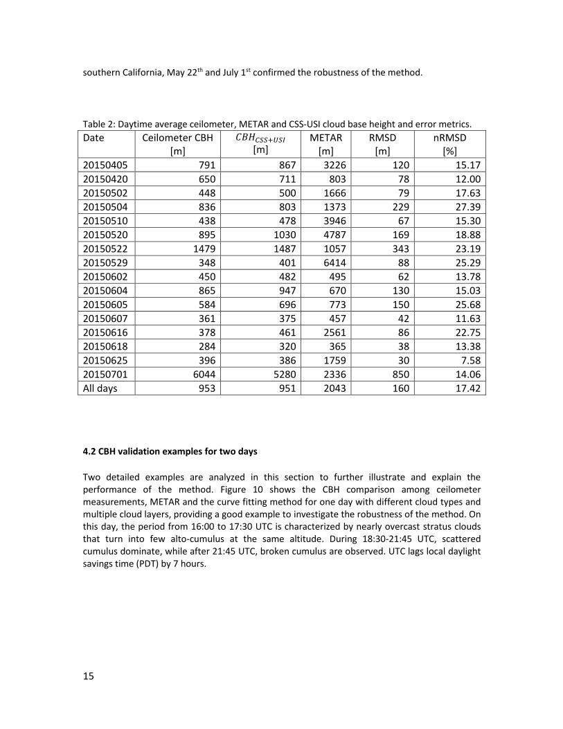
15

southern California, May 22th and July 1st confirmed the robustness of the method.

Table 2: Daytime average ceilometer, METAR and CSS-USI cloud base height and error metrics.

Date Ceilometer CBH [m]

𝐶𝐵𝐻𝐶𝑆𝑆+𝑈𝑆𝐼

[m] METAR

[m] RMSD

[m] nRMSD

[%]

20150405 791 867 3226 120 15.17

20150420 650 711 803 78 12.00

20150502 448 500 1666 79 17.63

20150504 836 803 1373 229 27.39

20150510 438 478 3946 67 15.30

20150520 895 1030 4787 169 18.88

20150522 1479 1487 1057 343 23.19

20150529 348 401 6414 88 25.29

20150602 450 482 495 62 13.78

20150604 865 947 670 130 15.03

20150605 584 696 773 150 25.68

20150607 361 375 457 42 11.63

20150616 378 461 2561 86 22.75

20150618 284 320 365 38 13.38

20150625 396 386 1759 30 7.58

20150701 6044 5280 2336 850 14.06

All days 953 951 2043 160 17.42

4.2 CBH validation examples for two days

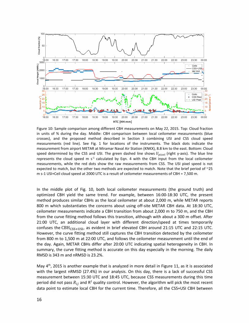
Two detailed examples are analyzed in this section to further illustrate and explain the performance of the method. Figure 10 shows the CBH comparison among ceilometer measurements, METAR and the curve fitting method for one day with different cloud types and multiple cloud layers, providing a good example to investigate the robustness of the method. On this day, the period from 16:00 to 17:30 UTC is characterized by nearly overcast stratus clouds that turn into few alto-cumulus at the same altitude. During 18:30-21:45 UTC, scattered cumulus dominate, while after 21:45 UTC, broken cumulus are observed. UTC lags local daylight savings time (PDT) by 7 hours.

16

Figure 10: Sample comparison among different CBH measurements on May 22, 2015. Top: Cloud fraction in units of % during the day. Middle: CBH comparison between local ceilometer measurements (blue crosses), and the proposed method described in Section 3 combining USI and CSS cloud speed measurements (red line). See Fig. 1 for locations of the instruments. The black dots indicate the measurement from airport METAR at Miramar Naval Air Station (KNKX), 8.8 km to the east. Bottom: Cloud speed determined by the CSS and USI. The green dashed line shows 𝑈𝑝𝑖𝑥𝑒𝑙 (right y-axis). The blue line

represents the cloud speed m s-1 calculated by Eqn. 4 with the CBH input from the local ceilometer measurements, while the red dots show the raw measurements from CSS. The USI pixel speed is not expected to match, but the other two methods are expected to match. Note that the brief period of ~25 m s-1 USI+Ceil cloud speed at 2000 UTC is a result of ceilometer measurements of CBH = 7,500 m.

In the middle plot of Fig. 10, both local ceilometer measurements (the ground truth) and optimized CBH yield the same trend. For example, between 16:00-18:30 UTC, the present method produces similar CBHs as the local ceilometer at about 2,000 m, while METAR reports 800 m which substantiates the concerns about using off-site METAR CBH data. At 18:30 UTC, ceilometer measurements indicate a CBH transition from about 2,000 m to 750 m, and the CBH from the curve fitting method follows this transition, although with about a 300 m offset. After 21:00 UTC, an additional cloud layer with different direction/speed at times temporarily confuses the CBHCSS+USI, as evident in brief elevated CBH around 21:15 UTC and 22:15 UTC. However, the curve fitting method still captures the CBH transition detected by the ceilometer from 800 m to 1,500 m at 22:00 UTC, and follows the ceilometer measurement until the end of the day. Again, METAR CBHs differ after 20:00 UTC indicating spatial heterogeneity in CBH. In summary, the curve fitting method is accurate on this day especially in the morning. The daily RMSD is 343 m and nRMSD is 23.2%. May 4th, 2015 is another example that is analyzed in more detail in Figure 11, as it is associated with the largest nRMSD (27.4%) in our analysis. On this day, there is a lack of successful CSS measurement between 15:30 UTC and 18:45 UTC, because CSS measurements during this time period did not pass 𝑅𝑖𝑗 and R2 quality control. However, the algorithm will pick the most recent

data point to estimate local CBH for the current time. Therefore, all the CSS+USI CBH between

17

16:00 to 18:45 UTC shown in the middle plot are calculated from a single data point that occurred on 15:38:58 UTC which is up to 3 hours earlier. This delay degrades the performance of the method. The same issue is observed after 23:00 UTC. These two periods are primarily responsible for the large RMSD. The periods with valid and recent CSS data show much better agreement with ceilometer measurements with typical differences less than 76 m. For example, around 19:00 UTC, the CSS+USI CBH follows a CBH transition and remains close to the ceilometer CBH thereafter. Thus, insufficient CSS data is another reason for poor performance of the curve fitting method.

Figure 11: Same as Fig. 10, but for May 4 illustrating a case when insufficient data points cause a large offset of local CBH estimates.

5. Discussion and Conclusions

The principal objective of this report is to introduce a sensor and an algorithm to provide an accurate local CBH for sky imager solar forecasting. The combination of a cloud speed sensor and sky imager makes measurements of CBH more affordable and convenient compared to a ceilometer. Ceilometers cost about $20k while the bill of material for the CSS is less than $400. Further a CSS could be directly integrated into the enclosure of a sky imager avoiding the need for separate setup site and power and Ethernet connectivity. On the other hand, a ceilometer is a fairly bulky and heavy instrument. First, a different assumption and algorithm are proposed and applied to the cloud speed sensor (CSS) introduced by Fung et al. (2014). The algorithm analyzes the similarity of signals, i.e. the correlation, in luminance between pairs of sensors aligned in different directions. Unlike prior methods that only considered the maximum correlation of the most correlated pair, the correlation coefficient of each pair of sensors is utilized to fit a cosine function. The approach is motivated by assuming a linear cloud edge passing over the sensor. If a good fit is observed, the cloud direction is determined by picking the angle with the maximum time delay of the cloud

18

passage on the cosine curve fit. The cloud speed is then equal to the sensor spacing divided by that time delay. CBH can then be derived by comparing CSS cloud speed measurements in [m s-

1] to cloud pixel speed in [pixel s-1] from a single sky imager. The improved CBH will be used in Task 3 of this project to produce improved sky imager solar forecasts to provide feed-forward control of a battery storage system that mitigates large ramp in solar generation. 16 days are analyzed with the proposed method. Overall, the method shows promising results with average nRMSD of 17.42% compared against on-site ceilometer measurements. Mathematically, the CBH accuracy depends on the accuracy of CSS cloud speed and the USI cloud pixel speed. Also, multiple layers of cloud with different direction and/or speed could degrade the performance because both CSS and USI are only able to determine cloud speed of one single cloud layer. In addition, the accuracy is restricted by the fact that the linear cloud edge assumption is based on the cloud motion vector being perpendicular to the cloud edge, which causes an underestimation of cloud speed. Lastly, the validation suffers from inconsistent measurement areas: (i) the ceilometer measures clouds straight overhead, (ii) the CSS detects the clouds that obscure the sun, and (iii) the USI analyzed clouds within its field of view that is typically about 10 km2. This could result in inconsistencies between the ceilometer and the CBH from the CSS and USI measurements.

Future efforts will focus on improving both CSS and USI cloud speed algorithms. CSS raw measurements could be filtered to remove irrelevant CMVs caused by sensor noise or irregular clouds. Also, USI cloud speed detection could be improved, for example using optical flow (Chow et al., 2015), to enable detection of multiple cloud layers as well as their respective cloud pixel speeds.

Acknowledgements We acknowledge a donation of a ceilometer from Lawrence Livermore National Laboratory that was facilitated by Julie Lundquist.

19

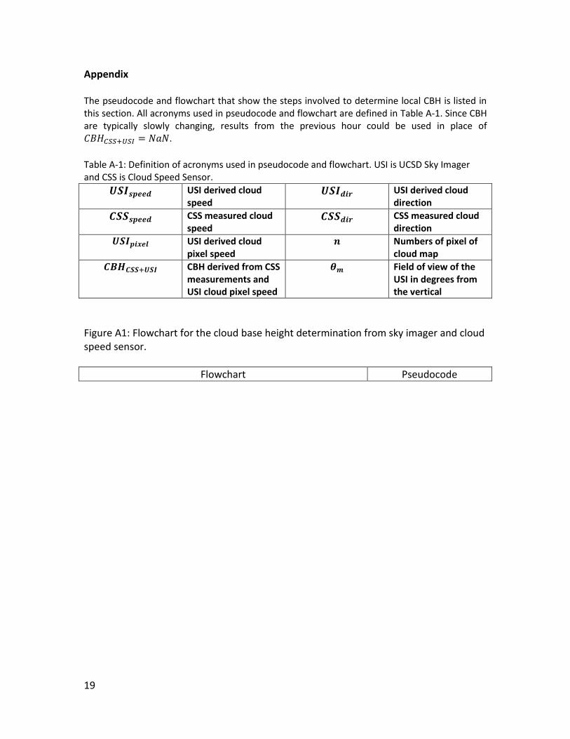
Appendix The pseudocode and flowchart that show the steps involved to determine local CBH is listed in this section. All acronyms used in pseudocode and flowchart are defined in Table A-1. Since CBH are typically slowly changing, results from the previous hour could be used in place of 𝐶𝐵𝐻𝐶𝑆𝑆+𝑈𝑆𝐼 = 𝑁𝑎𝑁. Table A-1: Definition of acronyms used in pseudocode and flowchart. USI is UCSD Sky Imager and CSS is Cloud Speed Sensor.

𝑼𝑺𝑰𝒔𝒑𝒆𝒆𝒅 USI derived cloud speed

𝑼𝑺𝑰𝒅𝒊𝒓 USI derived cloud direction

𝑪𝑺𝑺𝒔𝒑𝒆𝒆𝒅 CSS measured cloud speed

𝑪𝑺𝑺𝒅𝒊𝒓 CSS measured cloud direction

𝑼𝑺𝑰𝒑𝒊𝒙𝒆𝒍 USI derived cloud pixel speed

𝒏 Numbers of pixel of cloud map

𝑪𝑩𝑯𝑪𝑺𝑺+𝑼𝑺𝑰 CBH derived from CSS measurements and USI cloud pixel speed

𝜽𝒎 Field of view of the USI in degrees from the vertical

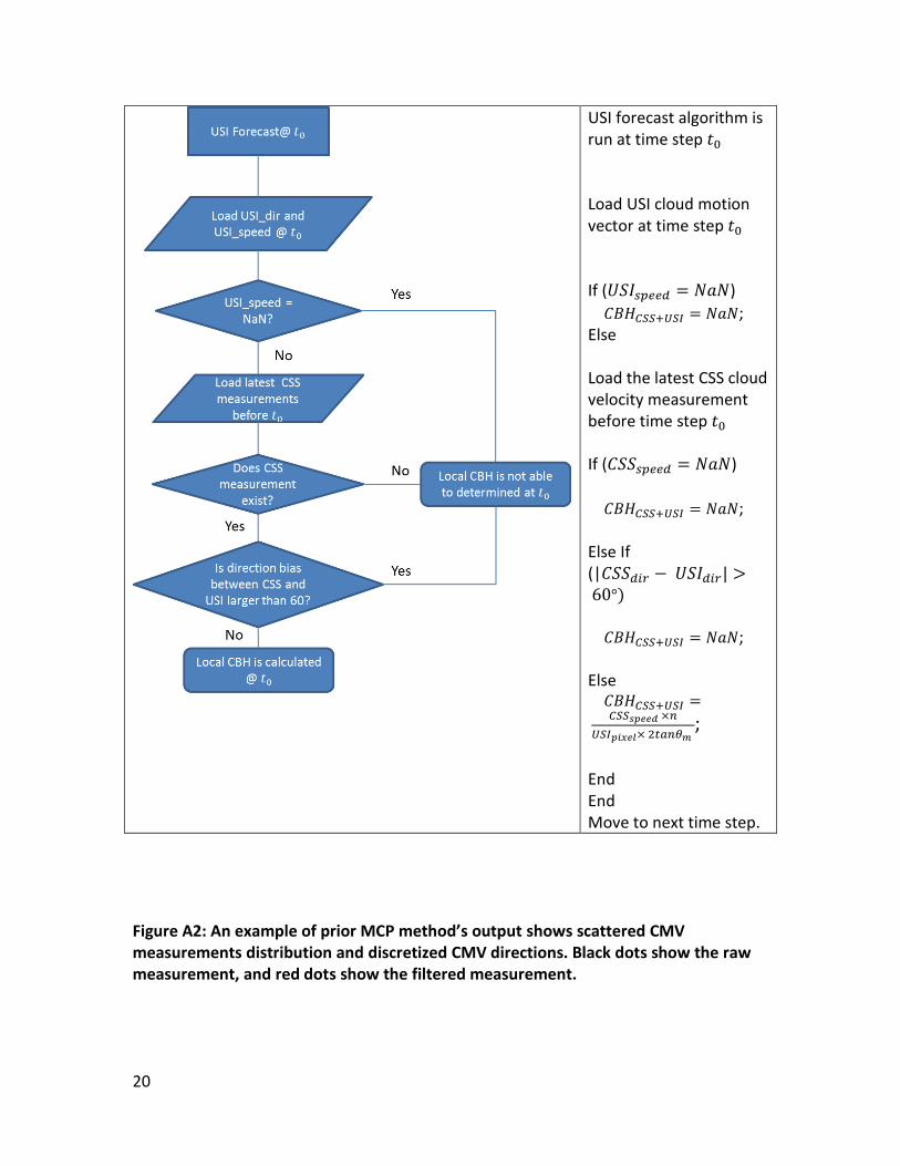
Figure A1: Flowchart for the cloud base height determination from sky imager and cloud speed sensor.

Flowchart Pseudocode

20

USI forecast algorithm is run at time step 𝑡0 Load USI cloud motion vector at time step 𝑡0 If (𝑈𝑆𝐼𝑠𝑝𝑒𝑒𝑑 = 𝑁𝑎𝑁)

𝐶𝐵𝐻𝐶𝑆𝑆+𝑈𝑆𝐼 = 𝑁𝑎𝑁; Else Load the latest CSS cloud velocity measurement before time step 𝑡0 If (𝐶𝑆𝑆𝑠𝑝𝑒𝑒𝑑 = 𝑁𝑎𝑁)

𝐶𝐵𝐻𝐶𝑆𝑆+𝑈𝑆𝐼 = 𝑁𝑎𝑁;

Else If (|𝐶𝑆𝑆𝑑𝑖𝑟 − 𝑈𝑆𝐼𝑑𝑖𝑟| > 60°)

𝐶𝐵𝐻𝐶𝑆𝑆+𝑈𝑆𝐼 = 𝑁𝑎𝑁;

Else 𝐶𝐵𝐻𝐶𝑆𝑆+𝑈𝑆𝐼 =

𝐶𝑆𝑆𝑠𝑝𝑒𝑒𝑑 ×𝑛

𝑈𝑆𝐼𝑝𝑖𝑥𝑒𝑙× 2𝑡𝑎𝑛𝜃𝑚 ;

End End Move to next time step.

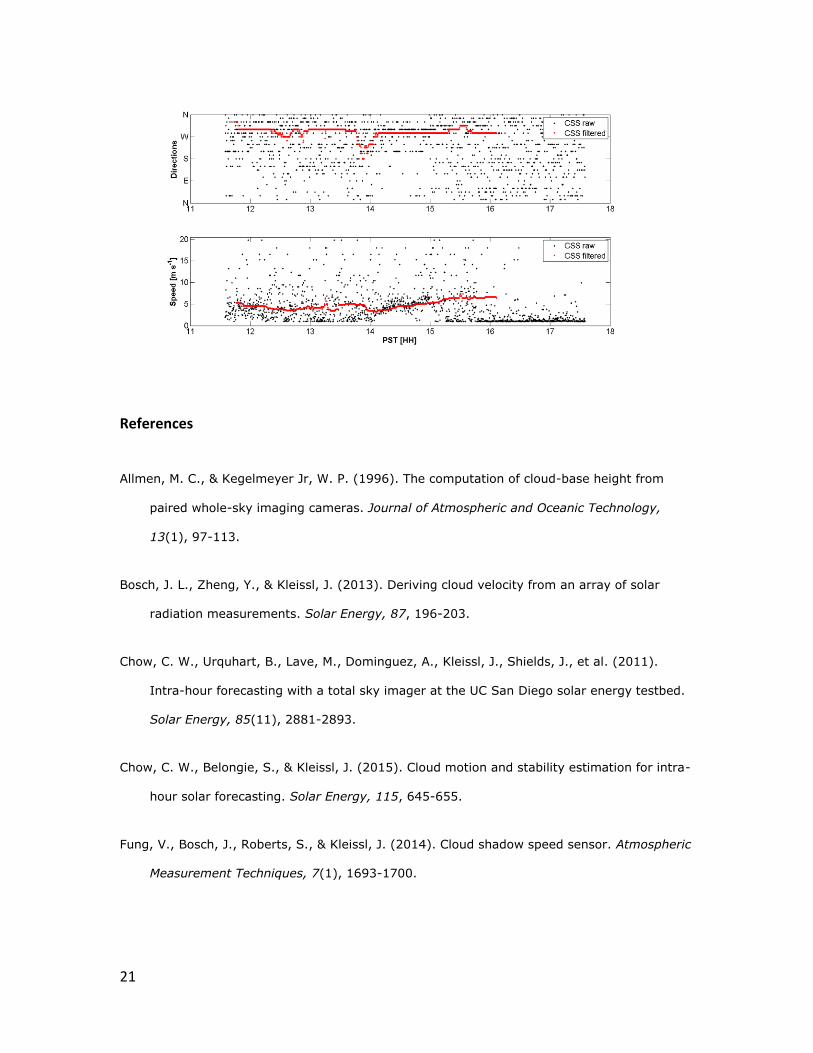
Figure A2: An example of prior MCP method’s output shows scattered CMV measurements distribution and discretized CMV directions. Black dots show the raw measurement, and red dots show the filtered measurement.

21

References

Allmen, M. C., & Kegelmeyer Jr, W. P. (1996). The computation of cloud-base height from

paired whole-sky imaging cameras. Journal of Atmospheric and Oceanic Technology,

13(1), 97-113.

Bosch, J. L., Zheng, Y., & Kleissl, J. (2013). Deriving cloud velocity from an array of solar

radiation measurements. Solar Energy, 87, 196-203.

Chow, C. W., Urquhart, B., Lave, M., Dominguez, A., Kleissl, J., Shields, J., et al. (2011).

Intra-hour forecasting with a total sky imager at the UC San Diego solar energy testbed.

Solar Energy, 85(11), 2881-2893.

Chow, C. W., Belongie, S., & Kleissl, J. (2015). Cloud motion and stability estimation for intra-

hour solar forecasting. Solar Energy, 115, 645-655.

Fung, V., Bosch, J., Roberts, S., & Kleissl, J. (2014). Cloud shadow speed sensor. Atmospheric

Measurement Techniques, 7(1), 1693-1700.

22

Ghonima, M., Urquhart, B., Chow, C., Shields, J., Cazorla, A., & Kleissl, J. (2012). A method

for cloud detection and opacity classification based on ground based sky imagery.

Atmospheric Measurement Techniques, 5(11), 2881-2892.

Hinkelman, L. M., George, R., Wilcox, S., & Sengupta, M. (2011). Spatial and temporal

variability of incoming solar irradiance at a measurement site in Hawai’i. 91st American

Meteorological Society Annual Meeting, pp. 23-27.

Yang, H., Kurtz, B., Nguyen, D., Urquhart, B., Chow, C. W., Ghonima, M., et al. (2014). Solar

irradiance forecasting using a ground-based sky imager developed at UC san diego. Solar

Energy, 103, 502-524.