design, optimization and validation of start-up sequences
TRANSCRIPT
HAL Id: tel-00765438https://tel.archives-ouvertes.fr/tel-00765438
Submitted on 14 Dec 2012
HAL is a multi-disciplinary open accessarchive for the deposit and dissemination of sci-entific research documents, whether they are pub-lished or not. The documents may come fromteaching and research institutions in France orabroad, or from public or private research centers.
L’archive ouverte pluridisciplinaire HAL, estdestinée au dépôt et à la diffusion de documentsscientifiques de niveau recherche, publiés ou non,émanant des établissements d’enseignement et derecherche français ou étrangers, des laboratoirespublics ou privés.
Design, optimization and validation of start-upsequences of energy production systems.
Adrian Tica
To cite this version:Adrian Tica. Design, optimization and validation of start-up sequences of energy production systems..Other. Supélec, 2012. English. �NNT : 2012SUPL0009�. �tel-00765438�
N° d’ordre : 2012-09-TH
THÈSE DE DOCTORAT
DOMAINE : STIC
SPECIALITE : AUTOMATIQUE
Ecole Doctorale « Mathématiques, Télécommunications, Informatique, Signal, Systèmes Electroniques »
Présentée par :
Adrian TIC; Sujet :
Conception, optimisation et validation des séquences de démarrage des systèmes de production d’énergie
Soutenue le 1 juin 2012 devant les membres du jury : M. Damien FAILLE EDF R&D Examinateur
M. Didier DUMUR SUPELEC Co-directeur de thèse
M. Eric BIDEAUX INSA de Lyon Rapporteur
M. Frédéric KRATZ ENSI de Bourges Président
M. Hervé GUEGUEN SUPELEC Directeur de thèse
M. Mohammed M’SAAD ENSI de Caen Rapporteur


Pentru fam ilia m ea...
“...the people who are crazyenough to think they can changethe world are the ones who do.”
Steve Jobs


Acknowledgments
The work reported in this thesis has been conducted in the Hybrid System Control Team(ASH) of the Supelec Rennes Campus. This research has been carried out in collaborationwith EDF (Electricite de France) and supported by the European 7th framework STREPproject ”Hierarchical and Distributed Model Predictive Control (HD-MPC)”, contractnumber INFSO-ICT-223854.
At Supelec, I have been fortunate to meet and work with wonderful people. Firstly, Iwould like to express my gratitude to my supervisor, Prof. Herve Gueguen, for giving methe opportunity to integrate the research project, and for the unequalled support over thelast three years. I can not put into words what I have learned from him. His intelligenceand attitude to research have been an important source of inspiration. I sincerely thankmy co-supervisor, Prof. Didier Dumur. His ability to synthesize, comments and advice,based on long experience in process control, have been very helpful. I am grateful for hisattention to detail and professionalism shown towards my work. It has been a huge honorto work and learn from them.
The participation in an international project was very interesting and challenging.I have had the opportunity to meet brilliant people, whose experience and knowledgehelped me to enrich my own theoretical and practical skills. Also, the collaboration andthe support provided by EDF’s experts have been a significant factor in the developmentof this research. I would like to express my gratitude to Dr.-Ing. Damien Faille, from EDFR&D, for his confidence in my work and results. His constant support and experiencein the modeling and the control of power plants have made an agreeable and rewardingcollaboration. I would also like to thank Ing. Frans Davelaar for his availability andassistance during my research. It was a pleasure to work with both of them.
I would like to express my most sincere gratitude to the members of my thesis com-mittee: Mr. Frederic Kratz, Professor at ENSI Bourges, who did me the honor of chairingthe examination committee, Mr. Eric Bideaux, Professor at INSA Lyon, and Mr. Mo-hammed M’Saad, Professor at ENSI Caen, who agreed to review this dissertation. I amvery grateful for their efforts to accomplish this work and for their constructive commentsand suggestions.
It was a very pleasant experience to work in the ASH Team. I would like to thank

iv
all team members: Jean Buisson, Herve Cormerais, Marie-Anne Lefebvre, Nabil Sadou,Pierre-Yves Richard and Romain Bourdais. All my colleagues: Antoine, Eunice, Ilham,Khang, Maxime, Mihai, Meriem, Soma, ... are acknowledged for creating a friendlyatmosphere and for all those scientific/non-scientific discussions during these years. DanielMorosan deserves my warmest thanks for his friendship, support and many unforgettablemoments experienced during this time.
I also wish to thank everybody from Supelec Rennes Campus who helped me through-out this thesis, and especially, to Catherine Pilet, Clairette Place, Gregory Cadeau,Ophelie Morvan and Myriam Andrieux for their administrative support and their kind-ness.
Working away from home and from loved ones is always a challenge. I have beenlucky to be surrounded by great friends here in Rennes, and I thank to: Alexandra,Alina, Anthony, Dali, Diana, Eliza, Rado, Remus, Roxana, ... I could not forget thosewho have supported me from back home. They are too many to be mentioned here.
A special thanks to my wonderful girlfriend, Raluca, for her love and support duringthis time.
Finally, and above all, I want to express all my gratitude and love to my parents and tomy brother. Thank you for your unconditional support and for giving me the opportunityto fulfill my dreams!
Adrian

Contents
Resume en francais xi
0.1 Contexte . . . . . . . . . . . . . . . . . . . . . . . . . . . . . . . . . . . . . xi
0.2 Centrale a cycles combines . . . . . . . . . . . . . . . . . . . . . . . . . . . xii
0.2.1 Description generale . . . . . . . . . . . . . . . . . . . . . . . . . . xii
0.2.2 Composants, configuration, fonctionnement . . . . . . . . . . . . . xii
0.2.3 Le processus de demarrage . . . . . . . . . . . . . . . . . . . . . . xiii
0.3 Modele physique de centrale . . . . . . . . . . . . . . . . . . . . . . . . . . xiv
0.4 Modele physique adapte pour l’optimisation . . . . . . . . . . . . . . . . . xv
0.4.1 Optimisation des modeles Modelica . . . . . . . . . . . . . . . . . . xv
0.4.2 Methodologie pour deduire modeles d’optimisation . . . . . . . . . xvi
0.4.2.1 Elimination des sources de discontinuite . . . . . . . . . . xvi
0.4.2.2 Bibliotheque ThermoOpt . . . . . . . . . . . . . . . . . . xvii
0.4.2.3 Validation des modeles de composants . . . . . . . . . . . xvii
0.5 Procedure d’optimisation du demarrage . . . . . . . . . . . . . . . . . . . xviii
0.5.1 Optimisation des trajectoires en boucle-ouverte . . . . . . . . . . . xviii
0.5.2 Resultats . . . . . . . . . . . . . . . . . . . . . . . . . . . . . . . . xix
0.6 Approche de commande predictive appliquee au processus de demarrage . xx
0.6.1 MPC approche pour l’optimisation du demarrage . . . . . . . . . . xx
0.6.2 Approche de commande predictive hierarchisee . . . . . . . . . . . xx
0.6.3 Resultats . . . . . . . . . . . . . . . . . . . . . . . . . . . . . . . . xx
0.7 Conclusions et perspectives . . . . . . . . . . . . . . . . . . . . . . . . . . xxii
Acronyms 3
1 Introduction 5
1.1 Background . . . . . . . . . . . . . . . . . . . . . . . . . . . . . . . . . . . 5
1.1.1 Electricity market . . . . . . . . . . . . . . . . . . . . . . . . . . . 8
1.1.2 Combined cycle power plant start-up optimization. Motivation . . 10
1.2 Dissertation objectives . . . . . . . . . . . . . . . . . . . . . . . . . . . . . 10

vi Contents
1.3 Organization and highlights of the dissertation . . . . . . . . . . . . . . . 11
2 Combined cycle power plants, start-up problem 132.1 Conventional Power Plants . . . . . . . . . . . . . . . . . . . . . . . . . . 132.2 Combined Cycle Power Plants . . . . . . . . . . . . . . . . . . . . . . . . . 15
2.2.1 General description . . . . . . . . . . . . . . . . . . . . . . . . . . . 152.2.2 CCPP features . . . . . . . . . . . . . . . . . . . . . . . . . . . . . 162.2.3 Configuration types of a combined cycle . . . . . . . . . . . . . . . 182.2.4 CCPP: Components, operation and control . . . . . . . . . . . . . 19
2.2.4.1 CCPP: Single pressure level . . . . . . . . . . . . . . . . . 202.2.4.2 Gas Turbine . . . . . . . . . . . . . . . . . . . . . . . . . 20
2.2.4.2.1 Description . . . . . . . . . . . . . . . . . . . . . 202.2.4.2.2 Local control strategy . . . . . . . . . . . . . . . 21
2.2.4.3 Heat Recovery Steam Generator . . . . . . . . . . . . . . 222.2.4.3.1 Description . . . . . . . . . . . . . . . . . . . . . 222.2.4.3.2 Local control strategy . . . . . . . . . . . . . . . 25
2.2.4.3.2.1 High Pressure Circuit . . . . . . . . . . . 252.2.4.3.2.2 Intermediate Pressure Circuit . . . . . . . 262.2.4.3.2.3 Low Pressure Circuit . . . . . . . . . . . 27
2.2.4.4 Steam Line . . . . . . . . . . . . . . . . . . . . . . . . . . 272.2.4.4.1 Description . . . . . . . . . . . . . . . . . . . . . 272.2.4.4.2 Local control strategy . . . . . . . . . . . . . . . 28
2.2.4.5 Steam Turbine . . . . . . . . . . . . . . . . . . . . . . . . 282.2.4.5.1 Description . . . . . . . . . . . . . . . . . . . . . 282.2.4.5.2 Local control strategy . . . . . . . . . . . . . . . 29
2.2.4.6 Condenser . . . . . . . . . . . . . . . . . . . . . . . . . . 302.2.4.6.1 Description . . . . . . . . . . . . . . . . . . . . . 302.2.4.6.2 Local control strategy . . . . . . . . . . . . . . . 30
2.2.4.7 GT and ST electrical generators . . . . . . . . . . . . . . 312.2.4.8 CCPP: Multi-pressure levels . . . . . . . . . . . . . . . . 31
2.2.5 CCPP start-up process . . . . . . . . . . . . . . . . . . . . . . . . 332.2.5.1 GT: Physical limitations and constraints . . . . . . . . . 352.2.5.2 HRSG: Physical limitations and constraints . . . . . . . . 35
2.2.5.2.1 High Pressure and Intermediate Pressure Circuits 362.2.5.2.2 Low Pressure Circuit . . . . . . . . . . . . . . . 36
2.2.5.3 SL: Physical limitations and constraints . . . . . . . . . . 372.2.5.4 ST: Physical limitations and constraints . . . . . . . . . . 372.2.5.5 Condenser: Physical limitations and constraints . . . . . 392.2.5.6 Start-up sequence . . . . . . . . . . . . . . . . . . . . . . 39
2.2.5.6.1 Preparation phase . . . . . . . . . . . . . . . . . 402.2.5.6.2 HRSG Start-up phase . . . . . . . . . . . . . . . 402.2.5.6.3 ST Start-up phase . . . . . . . . . . . . . . . . . 412.2.5.6.4 Increasing Load phase . . . . . . . . . . . . . . . 41
2.2.5.7 Objectives of start-up optimization . . . . . . . . . . . . 412.2.5.7.1 Minimization of start-up time . . . . . . . . . . 42
Contents vii
2.2.5.7.2 Minimization of the operating costs . . . . . . . 42
2.2.5.7.3 Minimization of material wear . . . . . . . . . . 42
2.2.5.7.4 Minimization of environmental impacts . . . . . 42
2.2.5.7.5 Minimization of start-up failure . . . . . . . . . 42
2.2.5.8 Approach to improve CCPP start-up . . . . . . . . . . . 43
2.2.5.8.1 New technological designs . . . . . . . . . . . . . 43
2.2.5.8.2 New approaches to improve start-up efficiency . 45
2.3 Conclusions . . . . . . . . . . . . . . . . . . . . . . . . . . . . . . . . . . . 50
3 Physical models for CCPP start-up 51
3.1 Modeling and Simulation . . . . . . . . . . . . . . . . . . . . . . . . . . . 51
3.2 Purpose of Modeling . . . . . . . . . . . . . . . . . . . . . . . . . . . . . . 53
3.3 Modelica language . . . . . . . . . . . . . . . . . . . . . . . . . . . . . . . 53
3.4 CPPP modeling . . . . . . . . . . . . . . . . . . . . . . . . . . . . . . . . . 56
3.4.1 Model libraries. Generalities . . . . . . . . . . . . . . . . . . . . . 56
3.4.2 ThermoPower library . . . . . . . . . . . . . . . . . . . . . . . . . 56
3.4.3 Models adapted to start-up phase . . . . . . . . . . . . . . . . . . 57
3.4.4 CCPP model . . . . . . . . . . . . . . . . . . . . . . . . . . . . . . 58
3.4.4.1 Model components description . . . . . . . . . . . . . . . 59
3.4.4.1.1 Gas Turbine model . . . . . . . . . . . . . . . . 59
3.4.4.1.2 Heat Recovery Steam Generator model . . . . . 59
3.4.4.1.3 Steam Turbine model . . . . . . . . . . . . . . . 64
3.4.4.1.4 Simplified component models . . . . . . . . . . . 66
3.4.5 Model initialization . . . . . . . . . . . . . . . . . . . . . . . . . . 66
3.4.6 Applicability of the CCPP model for optimization . . . . . . . . . 68
3.5 Conclusions . . . . . . . . . . . . . . . . . . . . . . . . . . . . . . . . . . . 69
4 CCPP models adapted for optimization 71
4.1 Introduction . . . . . . . . . . . . . . . . . . . . . . . . . . . . . . . . . . . 71
4.2 Modelica CCPP model suitable for optimization . . . . . . . . . . . . . . 71
4.3 Methodology to create smooth models . . . . . . . . . . . . . . . . . . . . 72
4.3.1 Elimination of discontinuity sources . . . . . . . . . . . . . . . . . 73
4.3.1.1 Approximation of conditional expressions . . . . . . . . . 73
4.3.1.2 Approximation of steam/water tables . . . . . . . . . . . 75
4.3.2 ThermoOpt library . . . . . . . . . . . . . . . . . . . . . . . . . . . 81
4.3.2.1 Library purposes . . . . . . . . . . . . . . . . . . . . . . . 82
4.3.2.2 Library principles . . . . . . . . . . . . . . . . . . . . . . 82
4.3.3 Library models validation . . . . . . . . . . . . . . . . . . . . . . . 86
4.3.3.1 Medium models validation . . . . . . . . . . . . . . . . . 87
4.3.4 Component models validation . . . . . . . . . . . . . . . . . . . . . 91
4.3.4.1 GT unit validation . . . . . . . . . . . . . . . . . . . . . . 92
4.3.4.2 HRSG unit validation . . . . . . . . . . . . . . . . . . . . 92
4.3.4.3 ST unit validation . . . . . . . . . . . . . . . . . . . . . . 93
4.3.5 Modelica CCPP smooth model . . . . . . . . . . . . . . . . . . . . 94
4.3.6 Model validation . . . . . . . . . . . . . . . . . . . . . . . . . . . . 96
viii Contents
4.4 Conclusions . . . . . . . . . . . . . . . . . . . . . . . . . . . . . . . . . . . 100
5 Start-up optimization procedure 101
5.1 Introduction . . . . . . . . . . . . . . . . . . . . . . . . . . . . . . . . . . . 101
5.1.1 Dynamic optimization . . . . . . . . . . . . . . . . . . . . . . . . . 102
5.1.2 Proposed solution . . . . . . . . . . . . . . . . . . . . . . . . . . . 103
5.2 Open-loop trajectory optimization . . . . . . . . . . . . . . . . . . . . . . 104
5.2.1 Gas Turbine load profile optimization . . . . . . . . . . . . . . . . 105
5.2.1.1 Problem formulation . . . . . . . . . . . . . . . . . . . . . 105
5.2.1.2 Parameterized functions . . . . . . . . . . . . . . . . . . . 107
5.2.1.2.1 Parameterization based on Hill function . . . . . 107
5.2.1.2.2 Basis functions . . . . . . . . . . . . . . . . . . . 108
5.2.1.2.2.1 Spline functions . . . . . . . . . . . . . . 108
5.2.1.2.2.2 GT load spline parameterization . . . . . 109
5.2.2 GT load profile and ST throttle opening profile optimization . . . 111
5.3 Results . . . . . . . . . . . . . . . . . . . . . . . . . . . . . . . . . . . . . . 112
5.3.1 Comparison standard sequence - optimal procedure . . . . . . . . . 113
5.3.1.1 Hill functions vs. classical profile . . . . . . . . . . . . . . 113
5.3.1.2 Spline functions application results . . . . . . . . . . . . . 115
5.3.1.2.1 Linear spline . . . . . . . . . . . . . . . . . . . . 115
5.3.1.2.2 Quadratic spline . . . . . . . . . . . . . . . . . . 116
5.3.2 Comparison minimum time - ”just-in-time” start-up problem . . . 117
5.3.3 GT load profile and ST throttle opening profile optimization . . . 118
5.3.4 Validation on the reference CCPP model . . . . . . . . . . . . . . 119
5.3.5 Start-up improvement benefits . . . . . . . . . . . . . . . . . . . . 120
5.3.6 Start-up optimization subproblem with Modelica-based platform . 122
5.3.6.1 Subsystem model . . . . . . . . . . . . . . . . . . . . . . 123
5.3.6.2 Optimization problem . . . . . . . . . . . . . . . . . . . . 123
5.4 Conclusion . . . . . . . . . . . . . . . . . . . . . . . . . . . . . . . . . . . 126
6 Model predictive approach for start-up procedure 129
6.1 Introduction . . . . . . . . . . . . . . . . . . . . . . . . . . . . . . . . . . . 129
6.2 Model predictive control . . . . . . . . . . . . . . . . . . . . . . . . . . . . 130
6.2.1 Concept . . . . . . . . . . . . . . . . . . . . . . . . . . . . . . . . . 130
6.2.2 Solution of the NMPC problem . . . . . . . . . . . . . . . . . . . . 132
6.3 GT load profile optimization. Predictive approach . . . . . . . . . . . . . 132
6.3.1 NMPC problem formulation . . . . . . . . . . . . . . . . . . . . . . 133
6.3.2 NMPC problem solution . . . . . . . . . . . . . . . . . . . . . . . . 134
6.3.3 Implementation of the predictive approach . . . . . . . . . . . . . 135
6.3.4 Simulation results . . . . . . . . . . . . . . . . . . . . . . . . . . . 136
6.4 Hierarchical model predictive control approach . . . . . . . . . . . . . . . 142
6.4.1 Hierarchical structure . . . . . . . . . . . . . . . . . . . . . . . . . 142
6.4.2 H-MPC problem formulation . . . . . . . . . . . . . . . . . . . . . 143
6.4.2.1 Optimization problem for the high level . . . . . . . . . . 143
6.4.2.2 MPC problem for the low level . . . . . . . . . . . . . . . 144

Contents ix
6.4.3 H-MPC multilevel algorithm . . . . . . . . . . . . . . . . . . . . . 1456.4.4 Results . . . . . . . . . . . . . . . . . . . . . . . . . . . . . . . . . 146
6.5 Conclusion . . . . . . . . . . . . . . . . . . . . . . . . . . . . . . . . . . . 151
7 Conclusions and perspectives 1537.1 Synthesis of the work . . . . . . . . . . . . . . . . . . . . . . . . . . . . . . 1537.2 Perspectives . . . . . . . . . . . . . . . . . . . . . . . . . . . . . . . . . . . 158
A Appendix: Modelica language 161
B Appendix: Modelica tools 171
C Appendix: CCPP identified model 175
D Appendix: Structure of the ThermoOpt library 181
E Appendix: Modelica components representation 183
F Appendix: CCPP Dymola diagram 187
G Appendix: Execution of Modelica/Dymola model in Matlab 191
List of Figures 195
List of Tables 197

x Contents
Resume en francais
0.1 Contexte
De nos jours, les producteurs d’electricite doivent repondre a des enjeux economiques etenvironnementaux de plus en plus eleves et s’adapter aux nouveaux modes de fonctionne-ment des systemes de production d’energies.
Actuellement, plus de la moitie des besoins mondiaux en energie electrique sont cou-verts par des centrales thermiques a combustibles fossiles. Parmis celles-ci, les cen-trales a cycles combines utilisent une technologie qui permet d’obtenir un rendementnettement superieur a celui des centrales classiques a combustible fossile, et d’assurerainsi une diminution considerable des emissions polluantes [1]. De plus, les installationsa cycles combines offrent plusieurs avantages economiques, avec entre autre, un coutd’investissement reduit et un temps de construction relativement court surtout vis-a-visdes centrales nucleaires.
C’est pourquoi ces dernieres annees, les centrales a cycles combines ont rencontreun fort succes et se sont developpees [2]. Elles representent le lien entre les anciennestechnologies de production basees sur la combustion des combustibles fossiles (destinees ajouer un role dominant dans le scenario de l’energie au moins jusqu’en 2030) et l’evolutionvers des sources novatrices et renouvelables d’energie.
Dans le contexte francais de l’energie electrique, ce type de centrale thermique estdestine a completer la production de base des centrales nucleaires en particulier lors despics de consommation. Elles sont donc demarrees et arretees relativement souvent pouroffrir ce service d’appoint. De plus, la deregulation du marche de l’electricite a introduit denouveaux producteurs sur le reseau, et des variations importantes du prix de l’electricitepeuvent etre constatees pendant une journee. Par consequent, les centrales sont soumisesa un nombre important des sequences demarrage/arret.
Ces transitoires, en particulier les demarrages, sont cependant delicats car ils con-duisent a un vieillissement accelere des equipements. Il est donc interessant de fournir unenouvelle strategie de gestion plus efficace qui permet d’optimiser le temps de demarragede la centrale, tout en respectant les contraintes de vieillissement des materiels.
L’objectif de cette these est de proposer une methode de conception, d’optimisationet de validation des sequences de demarrages qui permette de diminuer les temps et lescouts de demarrage tout en preservant la duree de vie, en respectant des contraintes qui

xii Resume en francais
limitent le vieillissement des composants physiques.La solution proposee consiste a effectuer l’optimisation du demarrage par une approche
basee sur un modele physique. En outre, les travaux ont porte sur l’application desapproches de commande predictive pour optimiser la sequence de demarrages des centralesa cycles combines.
Afin d’obtenir un fonctionnement sur et efficace, et en meme temps de pouvoir ex-ploiter pleinement le potentiel du processus, les methodes suggerees dans ce manuscritsont basees sur un modele physique precis de la centrale lors la phase de demarrage. Pourcela, une bibliotheque specialisee, basee sur un langage de modelisation physique a eteutilisee.
0.2 Centrale a cycles combines, la problematique du pro-
cessus de demarrage
0.2.1 Description generale
Les centrales a cycles combines sont des systemes thermodynamiques qui comportent deuxou plusieurs cycles de puissance, dont chacun utilise un fluide de travail different (d’oul’appellation cycles ”combines”) [3], [4], [5].
En general, cette technologie combine deux cycles thermodynamiques : elle associe lefonctionnement d’une turbine a combustion (cycle de Brayton) a celui d’une chaudiere derecuperation et d’une turbine a vapeur (cycle de Rankine). Les cycles mixtes vapeur/air(fluides de travail les plus communement utilises) fournissent un rendement eleve du faitque les deux cycles sont complementaires du point de vue thermodynamique : l’energiecalorifique des fumees issues de la turbine a combustion (TAC) est recuperee par lachaudiere, et constitue la source d’energie pour generer de la vapeur pour la turbinea vapeur (TAV).
L’utilisation du deuxieme cycle (eau-vapeur) peut avoir differentes finalites :
- production d’electricite ;
- production de vapeur pour un reseau de chauffage ou a des fins industrielles ;
- production de vapeur et d’electricite : cogeneration [6].
0.2.2 Centrale a cycles combines : structure, fonctionnement
Les installations a cycles combines presentent une large gamme d’options de design etde configurations en ce qui concerne le nombre d’unites, le type de chaudiere, le type deTAV, etc. La structure de base d’une centrale electrique a cycles combines contient lescomposants principaux suivants :
- Turbine a combustible (TAC) ;
- Chaudiere de recuperation ;
- Turbine a vapeur (TAV) ;

0.2 Centrale a cycles combines xiii
- Ligne vapeur ;
- Condenseur ;
- Generateur.
Dans ce document, le type de centrale etudie a une configuration typique 1-1-1 (une TAC,une chaudiere, une TAV). La representation schematique d’une telle centrale est illustreedans la Figure 1. Aussi pour l’objectif propose, une chaudiere et une turbine a vapeuravec un seul niveau de pression (haute pression) ont ete considerees.
Lig
ne V
apeur
Eau
EauCondenseur
G TAVTAC
Ch
au
diè
re
Vapeur HP
Vapeur HP
Vapeur BP
Vapeur HP
Fumées
Pompe
Combustible
Air
Figure 1: Schema d’une centrale a cycles combines de type 1-1-1
Le fonctionnement normal d’un tel circuit se presente comme suit : de l’air ambiantest comprime, puis melange avec du combustible et brule a une pression constante. Legaz a haute temperature et haute pression cree par la combustion est detendu dans laTAC pour generer une puissance mecanique. Les fumees issues de la TAC sont utiliseespour produire de la vapeur dans la chaudiere de recuperation. La vapeur produite estdetendue dans la TAV pour fournir une puissance supplementaire. La vapeur issue de laTAV (BP-basse pression) est collectee par un condenseur. Le cycle eau/vapeur est ferme,en alimentant la chaudiere avec de l’eau provenant du condenseur.
0.2.3 Le processus de demarrage
Le demarrage des cycles combines est une tache complexe, comportant plusieurs phaseset des conditions qui doivent etre respectees simultanement. La procedure de demarragedepend de chaque technologie utilisee, mais en general elle peut etre decomposee en quatreetapes principales :
1. Phase de preparation : cette premiere etape prepare l’allumage de la TAC ;
2. Phase de lancement de la chaudiere : cette phase correspond au conditionnementthermique, et son objectif est de demarrer la chaudiere afin d’obtenir les caracteris-tiques de la vapeur (temperature, pression, qualite) adaptees pour l’admission dansla TAV ;
3. Phase de lancement de la TAV : au cours de cet etape, la TAV est demarree parl’admission de vapeur ;
xiv Resume en francais
4. Phase de prise de charge : pendant cette derniere etape, la charge de la centrale estaugmentee jusqu’a la puissance nominale.
En general, les techniques classiques de demarrage sont assez conservatrices, en seconcentrant principalement sur la securite et la disponibilite plutot que sur l’efficacite del’operation. Ces procedures sont concues de maniere a preserver naturellement la dureede vie des composants de l’installation. Toutefois, afin de repondre aux exigences ducontexte concurrentiel actuel, sans compromettre la securite du fonctionnement, de nou-velles strategies efficaces de demarrage sont necessaires. Les nouvelles strategies doiventintegrer la fiabilite et la flexibilite du fonctionnement, et fournir la puissance attribueepar le dispatching economique dans un temps minimal, tout en satisfaisant les contraintesd’exploitation et en minimisant les couts.
Dans cette these le processus de demarrage de la centrale est traite comme un problemed’optimisation dynamique, consistant a trouver un profil optimal pour les variables decontrole qui minimise une fonction objectif et remplit un ensemble de contraintes im-posees par la dynamique de l’installation et par les principales variables du processus (enparticulier les stress thermiques et mecaniques).
L’optimisation de la procedure dans son ensemble exige de prendre en compte unsysteme hybride contenant des variables discretes et continues qui interagissent. Toutefois,afin de reduire la complexite de l’optimisation, le probleme a ete decompose en sous-problemes plus simples correspondant a chaque phase de demarrage. Ce document estcentre sur la derniere partie du processus, lorsque les deux turbines sont synchroniseeset connectees au reseau (Prise de charge). Cette phase est consideree comme la pluscritique, car l’impact du stress sur les composants est important, ce qui affecte fortementleur duree de vie.
0.3 Modele physique de centrale a cycles combines pour le
demarrage
L’optimisation du demarrage repose sur la determination d’une trajectoire sous con-traintes d’un systeme dynamique correspondant a la centrale. Pour realiser cette op-timisation il est donc necessaire de disposer d’un modele de l’installation.
Actuellement, les processus doivent fonctionner sous des specifications economiques etenvironnementales de plus en plus strictes. En general, ces exigences peuvent etre satis-faites lorsque les systemes fonctionnent sur une gamme large de conditions d’exploitationet, en particulier a proximite des limites de sa region d’exploitation admissible. Dansce contexte, pour decrire adequatement le comportement dynamique du processus, desmodeles non-lineaires sont necessaires. Ceci est d’autant plus vrai pour les centraleselectriques a cycles combines qui ont des comportements dynamiques fortement non-lineaires lors de leur demarrage.
Pour mener les etudes, nous avons construit un modele non-lineaire de centrale avec laconfiguration specifiee dans le chapitre precedent, en utilisant pour la modelisation le lan-gage Modelica [7] et l’environnement de simulation Dymola [8]. Modelica est un langageoriente objet pour la modelisation des systemes physiques de grande dimension, complexes
0.4 Modele physique adapte pour l’optimisation xv
et heterogenes. Ce choix permet en effet de construire un modele fiable en assemblant etconfigurant des composants a partir des bibliotheques dans une approche hierarchisee etstructuree. Le modele developpe utilise la bibliotheque libre pour la modelisation de cen-trales thermiques (ThermoPower [9]) et a ete parametre avec des donnees de conceptionet de fonctionnement d’une unite typique [10].
Dans ce document, nous sommes interesses a la realisation d’un modele physique dela centrale pouvant etre utilise pour l’optimisation de la sequence de demarrage. Ainsi,le modele developpe est adapte a l’etude du demarrage, c’est-a-dire qu’il est en mesurede representer la sequence de demarrage. La representation mathematique du systemeconsidere des modeles simplifies pour les elements non critiques pour l’optimisation dudemarrage (turbine a gaz, condenseur, etc). Pour les autres elements, il comprend descomposants dont le comportement est valable sur tout le domaine de fonctionnement etmodelise des caracteristiques telles que les stress thermiques et mecaniques lorsqu’ils sontles plus limitants.
Les equations du modele proviennent principalement du premier principe de la ther-modynamique (conservation d’energie, conservation de masse).
0.4 Modele physique de centrale adapte pour l’optimisation
0.4.1 Optimisation des modeles Modelica
Avec le langage Modelica, un grand nombre de modeles (lineaires, non lineaires, hybrides,etc.) peut etre decrit, et de nombreux outils performants permettent de les simulerfacilement. Par contre, l’optimisation de ces modeles est plus difficile. En effet, les outilspour l’optimisation statique et dynamique des modeles Modelica sont generalement peupuissants.
En raison de l’heterogeneite et de la complexite des modeles Modelica, l’optimisationest en general faite en traitant le modele comme une boıte noire : l’optimisation utiliseles resultats de simulations sans que la structure particuliere du modele ne soit exploreeselon des methodes heuristiques. L’objectif a donc ete d’etudier comment on pouvaitutiliser de tels modeles, en particulier le modele de la centrale developpe, pour appliquerdes algorithmes d’optimisation efficaces.
La classe d’algorithmes envisagee pour l’optimisation appartient aux methodes fondeessur les gradients. Cette classe peut traiter des systemes de grande echelle, en etant capablede resoudre des problemes de controle optimal sous conditions de temps reel. En general,l’application des methodes de gradient impose une serie de conditions sur la formulationdu modele, en particulier, celle de l’absence de sources de discontinuite (par exemple, lesstructures si-equations).
En ce sens, une methodologie a ete proposee. L’approche vise a obtenir des modelesModelica appropries pour l’optimisation avec des methodes basees sur le gradient. Lemodele du chapitre precedent est considere comme modele de reference. Celui-ci est aussiutilise pour realiser et valider des modeles adaptes pour l’optimisation.

xvi Resume en francais
0.4.2 Methodologie pour creer des modeles Modelica appropries pour
l’optimisation
0.4.2.1 Elimination des sources de discontinuite
Le principe de l’approche consiste a associer a chaque composant du modele initial,une version dans laquelle les sources de discontinuite sont approchees par le biais desrepresentations continues, en gardant ainsi la meme structure et une bonne precision dumodele.
En bref, les etapes accomplies dans l’approche sont les suivantes :
a) l’analyse des composants du modele de simulation et l’identification des sourcespotentielles de discontinuite ;
b) l’elaboration de composants du modele sans sources de discontinuites, en intro-duisant les representations continues ;
c) la validation des composants du modele.
Dans la phase de construction, la representation continue est basee sur l’utilisationd’une approximation de la fonction de Heaviside :
∀x ∈ R, H(x) =
{0, x < 0
1, x ≥ 0(1)
remplacee par l’approximation lisse :
∀x ∈ R, Hk(x) =1
1 + e−kx(2)
ou k est le coefficient de lissage (voir la Figure 2).
−2 −1.5 −1 −0.5 0 0.5 1 1.5 20
0.1
0.2
0.3
0.4
0.5
0.6
0.7
0.8
0.9
1
x
H(x
)
fonction de Heavisideapproximation
Figure 2: La fonction de Heaviside et son approximation pour k=20
0.4 Modele physique adapte pour l’optimisation xvii
L’utilisation d’une approximation lisse sert a rendre continues les discontinuites desstructures conditionnelles. Par exemple, pour un modele conditionnel Modelica commepresente ci-dessous :
hm = if h ≤ hl then hl else hv (3)
la representation continue est ainsi formulee :
f(h) =1
1 + e−k∗(h−hl)(4a)
hm =hv ∗ f(h) + (1− f(h)) ∗ hl (4b)
Un probleme specifique a ete la representation des tables de vapeur/eau. Ces modelesont ete estimes sur differents domaines thermodynamiques (regions), et ensuite raccordesde maniere lisse pour obtenir une representation continue.
0.4.2.2 Bibliotheque ThermoOpt
La methodologie proposee a permis de construire une bibliotheque de composants Mod-elica adaptes a l’optimisation a partir d’une bibliotheque standard Modelica concue pourla simulation. Un modele de la centrale, approprie pour l’optimisation, a ete construiten utilisant des composants provenant de la bibliotheque ThermoOpt. Le modele a lesmemes caracteristiques et la meme configuration que la representation a cycle combine dereference. Ainsi, le modele pour l’optimisation, peut etre deduit du modele de simulationpar simple substitution de la bibliotheque.
0.4.2.3 Validation des modeles de composants
L’ensemble des nouvelles versions des composants et le modele global de la centrale aete valide par comparaison en simulation avec les modeles originaux. Pour demontrer lacoherence des modeles de composants, plusieurs scenarios de simulation ont ete etudies.En general, la validation des elements de la bibliotheque d’optimisation a ete effectuee encomparant leurs reponses, aux variations des signaux d’entree, avec les reponses obtenuespar les modeles de reference.
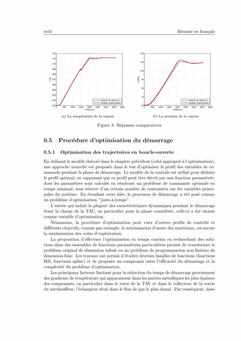
Quelques resultats de simulation pour une variation de type echelon du debit dudesurchauffeur et pour un profil de la charge de la TAC qui suit une rampe avec unepente d’environ 0,65%/min, appliquee apres 180 secondes, sont illustres dans la Figure 3.
Comme on peut le constater, les reponses du modele d’optimisation sont assez prochesde celles de reference. Par rapport au modele original, le comportement de la temperatureet de la pression de la vapeur dans la chaudiere se caracterise par une tres legere difference(erreur relative inferieure a 2.5%).
xviii Resume en francais
0 500 1000 1500 2000 2500 3000 3500 4000620
630
640
650
660
670
680
690
700
710
720
Temps [s]
T [K
]
Modèle de référenceModèle d’optimisation
(a) La temperature de la vapeur
0 500 1000 1500 2000 2500 3000 3500 400060
70
80
90
100
110
120
Temps [s]
p [b
ar]
Modèle de référenceModèle d’optimisation
(b) La pression de la vapeur
Figure 3: Reponses comparatives
0.5 Procedure d’optimisation du demarrage
0.5.1 Optimisation des trajectoires en boucle-ouverte
En utilisant le modele elabore dans le chapitre precedent (celui approprie a l’optimisation),une approche nouvelle est proposee dans le but d’optimiser le profil des variables de co-mmande pendant la phase de demarrage. Le modele de la centrale est utilise pour deduirele profil optimal, en supposant que ce profil peut etre decrit par une fonction parametree,dont les parametres sont calcules en resolvant un probleme de commande optimale entemps minimal, sous reserve d’un certain nombre de contraintes sur les variables princi-pales du systeme. En etendant cette idee, le processus de demarrage a ete pose commeun probleme d’optimisation ”juste-a-temps”.
L’entree qui induit la plupart des caracteristiques dynamiques pendant le demarrageetant la charge de la TAC, en particulier pour la phase consideree, celle-ci a ete choisiecomme variable d’optimisation.
Neanmoins, la procedure d’optimisation peut viser d’autres profils de controle etdifferents objectifs, comme par exemple, la minimisation d’usure des materiaux, ou encorela minimisation des couts d’exploitation.
La proposition d’effectuer l’optimisation en temps continu en recherchant des solu-tions dans des ensembles de fonctions parametrees particulieres permet de transformer leprobleme original de dimension infinie en un probleme de programmation non-lineaire dedimension finie. Les travaux ont permis d’etudier diverses familles de fonctions (fonctionsHill, fonctions spline) et de proposer un compromis entre l’efficacite du demarrage et lacomplexite du probleme d’optimisation.
Les principaux facteurs limitant pour la reduction du temps de demarrage proviennentdes gradients de temperature qui apparaissent dans les parties metalliques les plus epaissesdes composants, en particulier dans le rotor de la TAV et dans le collecteur de la sortiedu surchauffeur, l’echangeur situe dans le flux de gaz le plus chaud. Par consequent, dans

0.5 Procedure d’optimisation du demarrage xix
le probleme d’optimisation, des contraintes sur les valeurs maximales des contraintesthermiques et mecaniques dans le rotor et dans le collecteur ont ete imposees. En effet,ces pics determinent la consommation de la duree de vie pendant toute la sequence dedemarrage, sans tenir compte des effets additionnels causes par la variation du niveau destress (fatigue).
0.5.2 Resultats
Afin de montrer les avantages de l’approche proposee, une comparaison entre la per-formance du demarrage lorsque la procedure optimale est appliquee, et une sequenceclassique a prise de charge constante a ete effectuee. Le tableau 1 resume les resultatsobtenus.
Optimisation de la charge TAC
Fonction/ Temps de Gain de Economie de Opt. Temps
sous-intervalles (N) demarrage [s] temps1[%] carburant1[%] parametres calc. [s]
lineaire parN=1* 6038 - - 1 20
N=10 5540 ≈8 ≈8 10 561
morceaux N=20 4980 ≈17 ≈15 20 855
2-Hill 4466 ≈26 ≈30 6 169
splineN=3 4777 ≈21 ≈23 3 58
N=3v 4397 ≈27 ≈30 5 154
quadratique N=4v 4278 ≈30 ≈34 7 253
Optimisation de la charge TAC et de l’ouverture de la valve TAV
spline NTAC=4v4120 ≈32 ≈36 12 663
quadratique NTAV =3v
Probleme du demarrage ”juste-a-temps”
2-Hill 4510 ≈25 ≈29 5 321
splineN=4v 4321 ≈28 ≈31 6 388
quadratique
1 relativement a la procedure standard* correspondant a la procedure standard avec une rampe de la charge TAC de 2 MW/minv parametrage avec sous-intervalles variables
Table 1: Resultats de simulation/optimisation
Les resultats montrent que la nouvelle procedure optimale reduit considerablement letemps de demarrage, en consommant jusqu’a 36% de moins qu’un demarrage traditionnela prise de charge constante. En raison du fait que les outils pour l’optimisation statiqueet dynamique des modeles physiques, en particulier pour les modeles developpes dans lelangage Modelica, sont generalement peu puissants, les solutions proposees sont basees surun compromis entre l’efficacite du demarrage (par exemple, le temps de demarrage), d’unepart, et les performances de calcul (le temps de calcul, les proprietes de convergence),d’autre part.

xx Resume en francais
0.6 Approche de commande predictive appliquee au pro-
cessus de demarrage
0.6.1 MPC approche pour l’optimisation du demarrage
La derniere partie des travaux a ete centree sur l’utilisation de la demarche d’optimisationa temps continu precedemment presentee dans une strategie de commande a horizonglissant de type Model Predictive Control (MPC). Cette approche permet de corriger lesderives liees aux erreurs de modele et aux perturbations, d’une part, et de considerer pourl’optimisation a chaque instant d’echantillonnage une fonction plus simple conduisant aun meilleur compromis complexite/temps de demarrage, d’autre part. Cette approche decommande conduit cependant a des temps de calcul importants.
0.6.2 Approche de commande predictive hierarchisee
Afin de reduire le temps de calcul, une structure de commande predictive hierarchiseetravaillant a des echelles de temps et sur des horizons differents a ete proposee.
La structure comporte deux niveaux : haut (NH) et bas (NB). Au niveau haut unprobleme de controle optimal en temps minimal est resolu sur une longue periode detemps. La solution de ce probleme est utilisee pour mettre a jour la reference pour leniveau bas, ou un probleme de suivi de consigne sous contrainte est resolu sur une courteperiode (Tp).
L’idee derriere l’approche hierarchique a ete de creer une structure de controle avecdes problemes d’optimisation plus appropries en terme de temps de calcul.
0.6.3 Resultats
L’application d’une strategie de commande predictive permet d’ameliorer d’une manieresignificative les performances du demarrage. Dans le Tableau 2 les resultats obtenuspour deux scenarios sont presentes en faisant varier les parametres de controle (l’horizonde prediction Tp, les periodes d’echantillonnage pour chaque controleur Ts pour MPC,{Tl, Th} pour H-MPC, la constante Tk qui definit l’instant auquel le signal de referenceest envoye au niveau bas et le type de parametrisation pour la charge TAC).
Les profils de la charge TAC issues de la strategie de MPC sont adaptes a l’etat actueldu systeme et sont generes avec une capacite de prediction specifique. Ainsi, avec uneestimation precise de l’evolution future du comportement de l’installation, en particuliersur l’evolution du stress dans le rotor et dans le collecteur, le profile de la charge peutetre plus agressif, en reduisant le temps de demarrage sans depasser les limites admissibles(voir la Figure 4).
Cependant en raison de la complexite du probleme d’optimisation, la resolution enligne a chaque pas d’echantillonnage est assez difficile. A l’exception de quelques casparticuliers, le solveur n’est pas en mesure de fournir une solution dans un delai definiinferieur a la periode d’echantillonnage du processus.
L’algorithme hierarchise (H-MPC) fournit des solutions compatibles avec une implan-tation en temps reel. En outre, les performances du demarrage sont proches de celles

0.6 Approche de commande predictive appliquee au processus de demarrage xxi
donnees par le regulateur MPC avec un seul niveau. Neanmoins, l’application efficace del’algorithme en temps reel conditionne la precision avec laquelle le profil de charge TACest approxime.
Optimisation de la charge TAC
Approche Parametres de Temps de Gain de Economie de Temps calc.[s]
controle [s] demarrage [s] temps [%] carburant [%] total moyen
standard - - 6038 - - - -
spline- 4278 - - - -
quad.
MPCTs=60 Tp=3Ts 3600 ≈40* ≈43* 2884 48
S1
H-MPC Tl=60 Tp=3Tl3600 ≈40* ≈43* 1425
10.5NH
S1 Th=2Tl Tk=5Tp 18.2NB
MPCTs=60 Tp=3Ts 3240 ≈46* ≈48* 6218 115.1
S3
H-MPC Tl=60 Tp= 5Tl3240 ≈46* ≈48* 2949
9.6NH
S3 Th=3Tl Tk= 2Tp 51.2NB
* relativement a la procedure standardNH Temps de calcul moyen au Niveau HautNB Temps de calcul moyen au Niveau BasS1 Scenario 1 : MPC avec le profil de la TAC decrit par une fonction lineaireS3 Scenario 3 : MPC avec le profil de la TAC decrit par les polynomes de Lagrange
Table 2: Resultats comparatifs commande MPC
0 1000 2000 3000 4000 5000 60000.1
0.2
0.3
0.4
0.5
0.6
0.7
0.8
0.9
1
Temps [s]
Cha
rge
TA
C [n
orm
alis
ée]
MPCH−MPCboucle−ouverte : spline quadratique standard
point final
(a) Profils de la charge TAC
0 1000 2000 3000 4000 5000 60000
200
400
600
Temps [s]
Str
ess
du r
otor
[MP
a]
0 1000 2000 3000 4000 5000 600040
60
80
100
120
Temps [s]
Str
ess
du c
olle
cteu
r [M
Pa]
MPCH−MPCboucle−ouvertestandard
MPCH−MPCboucle−ouvertestandard
(b) Evolution des stresses
Figure 4: Resultats comparatifs de simulation. Pour les controleurs MPC, le parametragecorrespond au Scenario 1 du Tableau 2
xxii Resume en francais
0.7 Conclusions et perspectives
Cette these a ete consacree a l’elaboration de nouvelles strategies pour l’amelioration de laperformance du demarrage des centrales a cycles combines. Les strategies proposees sontbasees sur l’utilisation d’un modele physique du processus et de techniques d’optimisationdynamique pour la realisation des objectifs prevus. Dans la suite, les principales contri-butions de la these sont listees :
• Un premier apport consiste en une methodologie qui permet a partir d’une bib-liotheque Modelica, concue pour la simulation, de construire une bibliotheque adap-tee a l’optimisation. En utilisant des composants provenant de cette bibliotheque,un modele de centrale, approprie pour l’optimisation, a ete construit et valide.
• La suite des travaux porte sur l’utilisation du modele pour optimiser le temps dedemarrage d’une centrale a cycles combines. Le modele a ete utilise pour deduire leprofil optimal de la charge de la turbine a combustible, en supposant que ce profilpeut etre decrit par une fonction parametree, dont les parametres sont calcules enresolvant un probleme de commande optimale sous contraintes. La solution proposeeoptimise en temps continu le profil en recherchant l’optimum dans des ensemblesde fonctions particulieres (Hill, splines, ...). Les travaux ont precisement porte surl’etude de diverses familles de fonctions et sur le compromis entre la performance dudemarrage et la complexite de l’optimisation. En etendant cette idee, le processusde demarrage a ete pose comme un probleme d’optimisation ”juste-a-temps”.
• La derniere partie des travaux considere l’integration de la solution a temps con-tinu dans une commande a horizon glissant, de type predictive a modele non lineaire(NMPC). Cette approche en boucle fermee permet d’une part, de corriger les derivesliees aux erreurs de modele et aux perturbations, et d’autre part, d’ameliorer lecompromis entre le temps de calcul et l’optimalite de la solution. Une structurehierarchisee a 2 niveaux travaillant a des pas de temps et sur des horizons deprediction differents est finalement proposee pour reduire le temps de calcul.
L’ensemble des travaux a conduit a des resultats interessants tant sur le plan applicatif,avec une reduction importante du temps theorique de demarrage (jusqu’a 47% par rapporta une sequence a prise de charge constante), que sur le plan methodologique.
En prolongement de ces travaux de these, plusieurs directions peuvent etre envisageespour les developpements futurs. Les principales pistes sont les suivantes :
→ l’amelioration de la procedure d’optimisation par le calcul et la prise en compte desinformations derivees (par exemple, les gradients).
→ la conception d’un observateur en mesure de reconstruire les variables d’etat dusysteme en utilisant un modele physique Modelica/Dymola ; la consideration dessolutions robustes pour initialiser les modeles Modelica ;
→ l’etude de la robustesse des structures de commande proposees ;
→ l’extension de la bibliotheque ThermoOpt avec de nouveaux modeles de composants,et la modelisation des configurations reelles de centrales electriques.

Acronyms
API Application Programming Interface
APROS Advanced Process Simulation Software
ARX AutoRegressive with eXogenous variable
ATT Atemperator (Desuperheater)
BLT Block Lower Triangular
CCPP Combined Cycle Power Plant
CCFF Combined Cycle Fully Fired
DAE Differential Algebraic Equation
DASSL Differential Algebraic System Solver
DCS Distributed Control System
DSH Desuperheater
ECO Economizer
ECO-HP1 High Pressure first stage economizer
ECO-HP2 High Pressure second stage economizer
ECO-HP3 High Pressure third stage economizer
ECO-HP4 High Pressure fourth stage economizer
ECO-IP Intermediate Pressure stage economizer
ECO-LP Low Pressure stage economizer
2 Acronyms
EDF Electricite de France
ETS Emissions Trading System
EU European Union
EV Evaporator
EV-IP Intermediate Pressure Evaporator
EV-HP High Pressure Evaporator
EV-LP Low Pressure Evaporator
FEM Finite Element Method
G Generator
GT Gas Turbine
GTS Gas Turbine System
H-MPC Hierarchical Model Predictive Control
HAT Humid Air Turbine
HILS Hardware In the Loop Simulation
HL High Layer
HP High Pressure
HRSG Heat Recovery Steam Generator
IEA International Energy Agency
IAPWS International Association for the Properties of Water and Steam
IAPWS-IF97 IAPWS Industrial Formulation 1997
IGCC Integrated Gasification Combined Cycle
IGV Inlet Guide Vane
IP Intermediate Pressure
IPOPT Interior Point OPTimizer
ISE Integral Square Error
LdT Load Transducer (Sensor)
LL Low Layer

Acronyms 3
LP Low Pressure
LT Level Transducer (Sensor)
MPC Model Predictive Control
NMPC Nonlinear Model Predictive Control
Mtoe Million tones of oil equivalent
NLP Non-Linear Programming
OE Output Error
ODE Ordinary Differential Equation
PT Pressure Transducer (Sensor)
QP Quadratic Programming
RH-IP1 Intermediate Pressure first stage reheater
RH-IP2 Intermediate Pressure second stage reheater
RMSE Root Mean Square Error
SC Supercritical
SI International System of Units
SL Steam Line
SH Superheater
SH-HP1 High Pressure first stage superheater
SH-HP2 High Pressure second stage superheater
SH-IP Intermediate Pressure superheater
SH-LP Low Pressure superheater
SNOPT Sequential Non-linear OPTimizer
SpT Speed Transducer (Sensor)
SQP Sequential Quadratic Programming
ST Steam Turbine
STAG Steam and Gas
STIG Steam Injection Gas Turbine
TT Temperature Transducer (Sensor)
USC Ultra Supercritical

CHAPTER 1
Introduction
1.1 Background
During the last century, the continuous growth of the world’s population, the industrialdevelopment and the accelerated urbanization have resulted in a major energy demand,which is in full expansion. The energy affects the everyday life of each of us, and theincreased need for more energy will require in the next years massive investments andsubstantial improvement in energy efficiency, all while managing the risks associated withgreenhouse gas emission and climate change. The recent energy market liberalization,which aims the prices reduction, the security of supply, the improvement of efficiency andthe development of renewable energy production, through competition, is expected tohave a positive impact on economy and environment. The international agreements forclimate protection and energy security will involve major changes in the energy supplyand use, representing a fundamental challenge. The companies that produce energy andalso the whole society, in general, will undergo significant changes over the next decades,whether due to government intervention, increasing competition, limited resources orsimply public opinion.
Nowadays, at a global level, there is a strong relationship between economy and energy.As a result of the economic crisis and the global spread of its impacts, the future thatwill unfold in its wake faces unprecedented uncertainty. The strength of the economicrecovery holds the key to energy outlook for the following years.
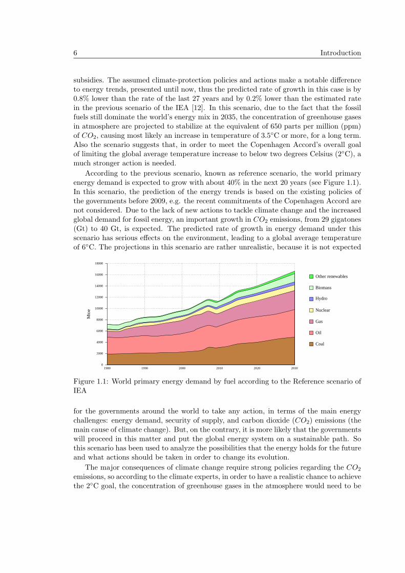
Although global energy demand has recently been reduced by economic recession, therecent annual projection [11] of the International Energy Agency (IEA), suggests that theworld primary energy demand might increase with about 36% between 2008 and 2035,from around 12300 million tones of oil equivalent (Mtoe) to over 16700 Mtoe (with 1.2%per year on average). This scenario takes into account the policy commitments and plansthat have been announced by the governments around the world, including the nationalpledges to reduce greenhouse gas emissions and future plans to phase out fossil-energy
6 Introduction
subsidies. The assumed climate-protection policies and actions make a notable differenceto energy trends, presented until now, thus the predicted rate of growth in this case is by0.8% lower than the rate of the last 27 years and by 0.2% lower than the estimated ratein the previous scenario of the IEA [12]. In this scenario, due to the fact that the fossilfuels still dominate the world’s energy mix in 2035, the concentration of greenhouse gasesin atmosphere are projected to stabilize at the equivalent of 650 parts per million (ppm)of CO2, causing most likely an increase in temperature of 3.5◦C or more, for a long term.Also the scenario suggests that, in order to meet the Copenhagen Accord’s overall goalof limiting the global average temperature increase to below two degrees Celsius (2◦C), amuch stronger action is needed.
According to the previous scenario, known as reference scenario, the world primaryenergy demand is expected to grow with about 40% in the next 20 years (see Figure 1.1).In this scenario, the prediction of the energy trends is based on the existing policies ofthe governments before 2009, e.g. the recent commitments of the Copenhagen Accord arenot considered. Due to the lack of new actions to tackle climate change and the increasedglobal demand for fossil energy, an important growth in CO2 emissions, from 29 gigatones(Gt) to 40 Gt, is expected. The predicted rate of growth in energy demand under thisscenario has serious effects on the environment, leading to a global average temperatureof 6◦C. The projections in this scenario are rather unrealistic, because it is not expected
1980 1990 2000 2010 2020 20300
2000
4000
6000
8000
10000
12000
14000
16000
18000
Mto
e
Other renewables
Biomass
Hydro
Nuclear
Gas
Oil
Coal
Figure 1.1: World primary energy demand by fuel according to the Reference scenario ofIEA
for the governments around the world to take any action, in terms of the main energychallenges: energy demand, security of supply, and carbon dioxide (CO2) emissions (themain cause of climate change). But, on the contrary, it is more likely that the governmentswill proceed in this matter and put the global energy system on a sustainable path. Sothis scenario has been used to analyze the possibilities that the energy holds for the futureand what actions should be taken in order to change its evolution.
The major consequences of climate change require strong policies regarding the CO2
emissions, so according to the climate experts, in order to have a realistic chance to achievethe 2◦C goal, the concentration of greenhouse gases in the atmosphere would need to be
1.1 Background 7
stabilized around 450 ppm of CO2 equivalent. To meet this stabilization target, the ’450’scenario of the IEA [13] estimates that the primary energy demand would grow with 20%,between 2007 and 2030, less than half than in the case of the reference scenario withoutclimate policy.
Despite the increased interest, manifested for renewable sources (hydro, wind, geother-mal, solar, etc.), the traditional energy sources, fossil fuels (coal, oil and natural gas), re-main largely dominant in all three scenarios of the IEA. Their share of the total primaryenergy mix varies depending on the scenario.
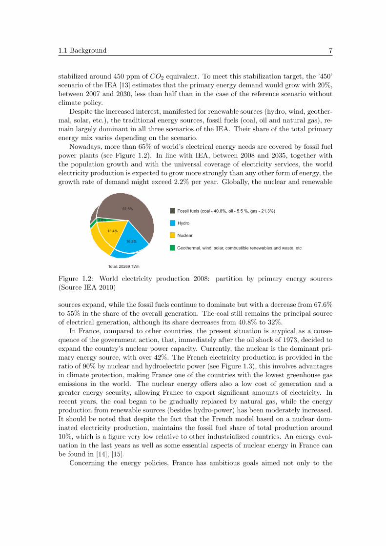
Nowadays, more than 65% of world’s electrical energy needs are covered by fossil fuelpower plants (see Figure 1.2). In line with IEA, between 2008 and 2035, together withthe population growth and with the universal coverage of electricity services, the worldelectricity production is expected to grow more strongly than any other form of energy, thegrowth rate of demand might exceed 2.2% per year. Globally, the nuclear and renewable
13.4%
16.2%
67.6%
2.8%
Total: 20269 TWh
Fossil fuels (coal - 40.8%, oil - 5.5 %, gas - 21.3%)
Hydro
Nuclear
Geothermal, wind, solar, combustible renewables and waste, etc
Figure 1.2: World electricity production 2008: partition by primary energy sources(Source IEA 2010)
sources expand, while the fossil fuels continue to dominate but with a decrease from 67.6%to 55% in the share of the overall generation. The coal still remains the principal sourceof electrical generation, although its share decreases from 40.8% to 32%.
In France, compared to other countries, the present situation is atypical as a conse-quence of the government action, that, immediately after the oil shock of 1973, decided toexpand the country’s nuclear power capacity. Currently, the nuclear is the dominant pri-mary energy source, with over 42%. The French electricity production is provided in theratio of 90% by nuclear and hydroelectric power (see Figure 1.3), this involves advantagesin climate protection, making France one of the countries with the lowest greenhouse gasemissions in the world. The nuclear energy offers also a low cost of generation and agreater energy security, allowing France to export significant amounts of electricity. Inrecent years, the coal began to be gradually replaced by natural gas, while the energyproduction from renewable sources (besides hydro-power) has been moderately increased.It should be noted that despite the fact that the French model based on a nuclear dom-inated electricity production, maintains the fossil fuel share of total production around10%, which is a figure very low relative to other industrialized countries. An energy eval-uation in the last years as well as some essential aspects of nuclear energy in France canbe found in [14], [15].
Concerning the energy policies, France has ambitious goals aimed not only to the

8 Introduction
13.3%77.1%
3.8%
4.8%
1%
Renewables 11.2%
1%
1%
0.1%
NuclearCoalGasOilHydroBiomassWindSolar, marine, waste, etc.
Figure 1.3: France electricity production 2008: partition by primary energy sources(Source IEA 2010)
energy security and competitive supply, but also the protection of the environment and theclimate, in order to reduce further the CO2 emissions (e.g. Grenelle Environment [16]). Inthe next years, the main targets with regard to sustainable development under EuropeanUnion (EU) 20-20-20 commitment by 2020 (20% improvement in energy efficiency, 20%reduction in greenhouses gas emissions and 20% renewable energy supply) [17] are:
• a reduction in CO2 emissions by 14% in the sectors outside Emissions TradingSystem (ETS);
• an increase in share of renewable energies to 23% of total energy consumption;
• a 20% reduction of the energy consumption, by improving energy efficiency.
All the predictions presented are based on scenarios covering demographic, geopoliticaland economic issues which involve risks and uncertainties, because they depend on certaincircumstances and are related to events, that will or may occur in the future. But beyondthe estimated figures, the information presented above offer us a large view about theglobal energy evolution.
1.1.1 Electricity market
The electricity is a form of energy which has become an essential part of today’s society.Every day the range and quantity of activities which need electrical energy are increasing.So the current energy production methods must cope with the demand growth and societyneeds. Briefly, we can expect important changes. The electricity industries all over theworld are undergoing a period of turmoil and transition. The way in which the electricityis generated, who are the producers, who financed its production, how it is distributed,how prices for it are calculated, they all are in a continuous change. Together with theelectricity technology evolution, the role of those involved (e.g. governments, electricityproducers, consumers, etc.), are changing.
A key aspect in the electric power markets is to ensure the stability and the relia-bility of the supply: due to its ”non storable” nature, the electricity must be produced,transmitted and consumed in real time. It means that suppliers have no inventory ofelectricity and have to be able to generate power at levels high enough to meet periods

1.1 Background 9
of peak consumption. Another problem is the market volatility, the large fluctuating indemand during the day requires a quick reaction from power generation plants to main-tain the balance between supply and demand. The achievement of a reliable electricitysupply and an efficient distribution was and remains a major priority.
In recent years a new priority has been set by the global efforts to deregulate theelectricity markets. Deregulation should improve the energy market, by opening the com-petition, offering more options and lower prices to the customers. The private companieshave begun to install their own power plants and supply electricity to the grid. Currently,the electricity manufacturers have to compete to sell their own product. If in a regulatedmarket, in the past, the companies obligations were to serve their customers with reliablepower, the cost minimization and profitability were considered as secondary endpoints,in this competitive context, overall production costs have become a key driver for theelectricity producers. The companies must offer electricity at the lowest cost, while stillfulfilling the requirements of grid stability and reliability.
The availability and the reliability of supply have an important role in economicalterms. Regarding the availability, if a unit is down, the producer has to either generatepower in another station or buy from another manufacturer. Anyway, both cases involveadditional costs. A high availability allows the operator to run a plant during longerperiods per year, resulting in higher returns. In terms of reliability, this is crucial inderegulated markets. During peak times, an important part of the income is generated,so the plant must be reliable. Also in order to limit losses, the outages can be scheduledoutside of peak hours, when costs are lower.
The market risks that can affect the investments (e.g. the price for electricity thatchanges every hour depending on supply and demand, unexpected costs of complyingwith greenhouse gas emission reduction regulations, uncertain future fuel costs, etc.)are accepted by the companies which expect that their plants will be competitive andthat they get an important profit during their exploitation. The deregulation createsa more dynamic environment where the risks and its minimization have a significantweight. As the risks mitigation is paramount, the investments in new and expandedpower stations are performed in close consultation with public policymakers, regulators,and other stakeholders. In this context, the electricity generators are focused to buy orbuild plants technologies with an industrial maturity and competitive costs. It should benoted that in many cases, the building of new plants, with long construction times andhigh capital costs, is considered more hazardous from the private investor’s point of view,so the use of the existing technologies is more interesting.
An attractive solution is the combined cycle technology [1]. The global electricitysupply industry admits that the first choice as production technology for the privateinvestors is represented by the combined cycle power plants (CCPPs), because of theiroutstanding advantages such as high efficiency and low environmental impact. Also thistechnology provides several economic advantages, including low investment costs andshort construction times compared to the conventional power plants, and even more thanthe nuclear plants offer.

10 Introduction
1.1.2 Combined cycle power plant start-up optimization. Motivation
In recent years, several new combined cycle plants have been installed and many existingunits have been re-powered [2]. The continuously growing number of CCPPs installed inthe world, together with the increasing energy demand and the competition for energydispatch to deal with deregulated power markets, require the development and the im-plementation of innovative strategies, either for control at partial or full load, or for thestart-up/shut-down phases.
This second topic is of great importance since in the current context, as a result ofcompetition among energy providers and daily fluctuations in power demand, CCPPs areundergoing frequent start-up/shutdown operations. Indeed, depending on their profitabil-ity, the combined-cycle units are shut down for short periods of time or for longer periods.Thus, during operation, these power plants are subject to a large number of transients.Furthermore, considering the fact that the start-up process is only a cost factor (no elec-trical power is delivered), and that the lifetime consumption of the plant components isseverely affected by the thermal and mechanical stresses reached during this phase, thecontrol and optimization of the start-up process represent a major interest.
In general, the traditional start-up techniques are quite conservative, being focusedmainly on safety and availability rather than on efficiency of the operation. These pro-cedures are designed in order to naturally preserve the lifetime consumption of the plantcomponents. However, in order to meet the requirements of the present competitive con-text without compromising the safe operation, efficient start-up strategies are necessary.The new strategies have to ensure reliability and flexibility in operation, and to deliver thepower assigned by the economic dispatch in minimal time, while satisfying the operatingconstraints and minimizing the costs.
Summarizing, the proposed research is motivated by the need to improve the efficiencyof combined cycle power plants start-up so as to meet tighter economical and environ-mental specifications, and to cope with stringent competition induced by the deregulationof energy market.
1.2 Dissertation objectives
Driven by the need to deal with a number of factors such as increased production demand,tight competition and new environmental policies, the main objective of this dissertationis to investigate and propose new methods to improve the CCPP start-up performances,while fulfilling constraints imposed on the physical process variables. The proposed solu-tion is to perform the optimization of the start-up of the combined cycle plants by meansof a model-based approach. Moreover, the optimal design of the start-up procedure isconsidered by means of a model-based predictive approach, the goal being to create aframework for control of the CCPP start-up.
In order to achieve safe and efficient operation, and at the same time to be able toexploit the full potential of the process, the suggested methods are based on an accuratephysical model of the plant. For this purpose, a dedicated modeling language togetherwith a specialized library are used.
1.3 Organization and highlights of the dissertation 11
The goal of this work is not only to investigate and propose new start-up controlstrategies, but also to emphasize the fact that the availability of a reliable, nonlinearmodel of a plant can represent an important tool for the design of efficient managementstrategies and advanced control techniques.
The modeling approach presented in this dissertation is aimed at allowing practitionersto develop and use operational physical simulation models built on the expert’s knowledge,for model-based control applications. The proposed methodology also serves as a meansof transforming existing knowledge-based models into optimization-oriented models.
1.3 Organization and highlights of the dissertation
The dissertation content is organized as follows:
Chapter 2
The second chapter presents a general overview of the combined cycle power plants. Itcovers important aspects of power plant design, operation, and optimization. The contentof this chapter is focused on the operation of a particular CCPP during the start-upphase, and defines the control specifications for this phase. Thus, plant is partitioned insubsystems and for each subsystem the operational constraints and the existing controlloops are indicated. The start-up procedure is described, and the objectives which canbe envisaged by the start-up optimization are discussed. A state of the art of the designtechnologies and approaches used for the optimization of the start-up process concludesthe chapter.
Chapter 3
In the third chapter the framework for achieving a physical model of a combined cycleplant is given, with a brief description of the dedicated modeling language and the libraryfor thermo-power systems used to develop process models. The Chapter 3 describes acombined cycle plant model built by using the Modelica language and the ThermoPowerlibrary. The model is based on the first principle laws and adapted to the start-up phase.The plant data are derived from a detailed simulator used to study the start-up of a realplant and the global behavior of the model has been validated by experts in the domain.Due to their modeling features and complexity the direct use of physical Modelica modelfor optimization purposes is often difficult. The study presented in this chapter willrepresent a first step towards achieving suitable models for optimization.
Chapter 4
In order to obtain a model that can be handled by efficient nonlinear algorithms for opti-mization and control purposes, a methodology is given in Chapter 4. The method aims attransforming the physical model developed in Chapter 3, considered as a reference plant,into an optimization-oriented model. The principle of the method is based on the refor-mulation of the plant model initially presented with discontinuity sources into a smooth

12 Introduction
model by means of continuous approximations of the Heaviside function. Based on thederived model components, a new optimization-oriented library for the modeling of com-bined cycle power plants is developed. Results of validation are presented to demonstratethe consistency of the model components and to emphasize the accuracy of the smoothCCPP model developed for optimization, compared to the original representation.
Chapter 5
A model-based approach to carry out the optimization of the combined cycle plantsstart-up phases, with focus on the last phase, is proposed in Chapter 5. The approachseeks to find an optimal profile of the control variables, in particular of the gas turbineload, by assuming that these profiles can be described by a parameterized function. Theparameters used for the profile-function description are computed by solving an optimalcontrol problem, subject to the plant dynamics represented by the Modelica/Dymolaoptimization-oriented model and to a number of constraints on the main plant variables,such as pressures, temperatures and stresses. Constrained by the lack of tool support fordynamic optimization relied on Modelica models, the suggested procedure is designed toachieve a good compromise between reliability, optimality of profile and computationalefficiency.
Chapter 6
The sixth chapter extends the approach already suggested by implementing a model pre-dictive control strategy. Formulating the start-up problem by means of a MPC controllermakes possible to exploit the features of this advanced control strategy (such as, itsprediction capability and ability to explicitly handle constraints, its built-in robustnessproperties) in order to derive fast GT loading rates, which lead to the reduction of thetransient time. However, due to the computational effort the application of MPC underreal-time conditions is limited. In the second part of the chapter, the MPC frameworkis redesigned to make it suitable for control of CCPP start-up process under real-timerequirements. Specifically, a hierarchical predictive structure with two layers is proposedin which a controller at each level deals with a specific objective.
Conclusions and perspectives
The last chapter reviews the research works presented in this manuscript, and offersseveral perspectives for future developments.
Appendixes
This manuscript contains several Appendixes in order to complete the content of thework, and to enable the reader to become familiar with the addressed topics.

CHAPTER 2
Combined cycle power plants, start-up problem
2.1 Conventional Power Plants
The thermal power plants represent one of the major sources of power generation. In athermal power plant, the electricity is produced by converting successively the chemicalenergy stored in primary sources (fossil fuels such as coal, oil, natural gas, etc) or thenuclear energy, in thermal energy, mechanical energy and finally in electrical energy. Thethermal-mechanical energy conversion is performed by means of gas turbine (GT) powerplants or steam turbine (ST) power plants, while for the mechanical-electrical conversion,the generators are used. The transformation of the chemical energy in thermal energy iscarried out in the furnace of the steam generator (boiler), for steam power plants and inthe combustion chamber, in the case of the gas turbine power plants [18], [19], [20], [21].Regarding the steam turbines, these use a separate heat source and do not directly convertfuel to electric energy. The energy is transferred from the boiler to the turbine throughhigh pressure steam. In other words, the steam turbine plants generate electricity as aby-product of heat (steam) generation, unlike the gas turbine plants, where the heat is aby-product of power generation. In general, ST plants can achieve an efficiency of over40% and their capacity can vary from 50 kW to several hundred MWs for large utilitypower plants.
Over time, the GT installation, used mainly in aviation, suffered a considerableprogress in order to reach powers unit comparable with other forms of energy production.Thus, the plants based on GT can cover a wide domain of electrical power production(from 3 to over 270 MW) and can reach up to 40% efficiency, even more for the modernunits. Nowadays, the GT plants are used rather to cover the peak electricity demand anddue to their short start-up time, these have a significant role in emergency services. BothGT and ST power plants offer a wide variety of designs and complexity [19], [18], in orderto improve the efficiency and/or to assure the performance specifications.
The GT and ST technologies are based on two thermodynamic cycles: the Joule cycle
14 Combined cycle power plants, start-up problem
or Brayton cycle and its derivatives which describe the operation of a gas turbine en-gine; the Rankine cycle and its derivatives (such as Rankine-Hirn cycle with overheating)which describe the thermodynamic transformations of the water-steam cycle of a steampower plant. In the following only the basic ideas of the thermodynamic cycles and plantoperation are presented, a complete description can be found in [4], [22], [19], [20], [18].
As a comparison between the GT and ST plants, besides the fact that each technologypresents advantages and disadvantages (e.g. GT plants offer an investment cost lower thanST plants, ST plants can operate with a large variety of fuels, GT has a simple designsince no boilers and their auxiliaries are required, GT can be started quickly from initialconditions, etc.), an essential difference is that for two turbines with the same size, theST will provide an electric power significantly larger than the GT.
For many years, in the past, the conventional steam power plants represented thefirst option to use fossil fuels to produce electricity. At that time, the thermal plantsalready used steam turbines with reheating and high steam parameters (170-180 bar, 540-560◦C). Currently, these plants represent about 30% of installed capacity and still remainpredominant over the world, because of their efficiency and their power unit significantlylarger than that the power stations based on GT. A large part of nuclear plants use alsothe thermal-mechanical energy conversion based on a steam cycle with lower temperaturesand pressures.
Initially, the construction of such power plants aimed mainly the electricity productionwith a minimal cost investments, and the issues as the reduction of the environmentalimpact and maximization of the efficiency, were not priorities. Nowadays, thermal powerplants offer a high availability and a low rate of unplanned or forced outage. In addition,the environment protection has become a priority.
Normally, the average lifetime of a conventional plant is of 30 to 40 years, but insome cases even after this period, the plant components can be in excellent operatingconditions. Consequently, a significant number of thermal power plants (which startedcommercial operation in years 1970 -1980) are currently in a technical state that allowstheir to operate in acceptable conditions for another 10 to 15 years. However, theseplants can not meet the current requirements in terms of efficiency and impact on theenvironment, so a rehabilitation is needed.
Concerning the rehabilitation of existing plants, there are different techniques, de-pending on several factors such as the topological conditions, the constructive features,the technical conditions, the life of major equipments, etc. One of the most attractivesolutions is to use the GTs [5], [2]. Repowering of the conventional steam plants bycompleting with a GT is synthesized to the development of particular combined cycleplant.
Over the last years, the improvement of the systems efficiency and the concept of sus-tainable development related to environmental protection, had to seek more efficient so-lutions in energy consumption and power plants with significantly improved performance.The improvement of the material quality and the technological evolution have led to aconsiderable increase in efficiency and productivity of the thermal power plants. More-over, high efficient cycles are available: the units designed for combined cycles (gas-steam)or conventional supercritical steam parameters, which provide performance considerably

2.2 Combined Cycle Power Plants 15
higher than the conventional units. For example, the implementation of Supercritical (SC)and Ultra Supercritical (USC) power generation technologies [23], [24], [25], the plantswhich operate at temperatures and pressures above the critical point of water, provideshigh efficiency (over 45%), with minimum fuel consumption and gas emission, as well as areliable supply of electric energy at low cost. Also, the combined cycle plants based on thenew technologies of turbines, give an efficiency up to 60%, which in terms of the environ-ment, contributes to the minimization of greenhouse gas emission [26]. Furthermore, thenew combustion techniques implemented in the GT technologies allow to achieve lowerrates of emissions of NOx and other pollutants [27], [28], [29]. Nevertheless, the most ofcombined cycle installations use fuels whose estimated reserves are low and their cost isuncertain on a long term (e.g. use natural gas as the main combustible for the GT).
An interesting solution, developed in recent years envisage the coal exploitation, af-ter the gasification process, in so called Integrated Gasification Combined Cycle (IGCC).IGCC technology converts the coal into a cleaner burning synthesis gas (syngas) and asits name suggest, combines the coal gasification with combined-cycle technology. Actu-ally IGCC represent the most efficient and clean way to use the coal for the electricityproduction [30], [31], [32], [33].
Currently, thermal power plants have to be flexible to meet rapidly fluctuations ofdemand levels, as well as to remain reliable, by minimizing the environmental impactsand maximizing the efficiency. So, in the industry, the new challenges are to ensure theflexibility and reliability of the operation with minimum forced outages and the lowestpossible costs, implementing innovative strategies that reduce CO2 emissions and dealwith deregulated power markets.
Despite the fact that the current trends target in particular renewable energy sources[34], the new energy technologies will not replace the large conventional units over theshort- to medium-term. Energy infrastructure takes time to develop and even longerto achieve the necessary industrial competitiveness and reliability. Therefore the energyproduction will rely for a long time period on the use of fossil fuels. In this context thecombined cycle plants and all technologies that emerge from it (e.g. IGCC), will mostlikely meet a strong growth in the coming years.
2.2 Combined Cycle Power Plants
2.2.1 General description
Combined Cycle Power Plant (CCPP) is an advanced power generation technology thatuses two or more thermodynamic cycles, in order to improve the efficiency [3], [4], [35],[5], [18], [36]. They represent the connection between the energy production technologiesbased on fossil fuels (which seem to be destined to play a dominant role in the energyscenario at least until 2035, according to IEA) and the evolution towards renewable andinnovative sources of energy.
In general, this technology combines the operation of a gas turbine Brayton cycle withthat of a steam turbine system Rankine cycle, using air and steam as working fluids. Thesteam/air combined cycles (the most used working fluids) provide an increased thermal
16 Combined cycle power plants, start-up problem
efficiency because the two cycles are complementary in terms of thermodynamic: theheat generated by the GT (Brayton cycle) has a temperature that is conveniently usedas energy source for the steam turbine system (Rankine cycle). In addition, the workingfluids (air and steam/water) are inexpensive, widely available and non-toxic.
The idea to exploit the second cycle has come from the fact that more than 60% ofthe thermal energy generated by Brayton cycle is rejected through the exhaust. So, byusing the ST a part of the exhaust gas energy generated by the gas cycle is recovered,enabling to obtain higher efficiencies than a GT alone (simple cycle configuration). Theconnection between the GT and the ST is performed by means of a Heat Recovery SteamGenerator (HRSG), that uses the hot gases exhaust from the GT to produce steamthat can be expanded in the ST, to generate additional power. The challenge in thesesystems is to obtain an integration level that maximizes the efficiency at an economic cost.Furthermore, the water-steam cycle, which recovers energy can have different purposes:
• power generation only;
• production of steam for urban heating network or for industrial purposes;
• simultaneous production of steam and electricity: cogeneration [6].
2.2.2 CCPP features
CCPPs represent the most efficient, reliable and economic method of power generationfrom fossil fuels, currently available. For these reasons, the combined cycle technology isone of the first options for most of the new power plants installed in the world.
The CCPPs commercially available today achieve a net thermal efficiency up to 60%.Further, the recent developments in GT materials and technology to sustain higher firingtemperatures and higher pressure ratio [37], have led to efficiency records of more than60% [38]. The constant technological development of the GT as well as the performanceimprovement of the steam cycle, is expected to lead to a higher efficiency. Efficiencyratings are very important in economic terms because over a 20-year project life, thecost of fuel represents about 70% of the operating cost for a CCPP. Thus, the efficiencyimprovements can provide considerable savings in fuel cost for the plant operators andlower electricity rates for the customers.
A high efficiency with regard to fuel resource consumption also means that moreelectricity can be generated with less environmental damage. So, another major advan-tage corroborated with the improved performance is the significant reduction in pollutantemissions [39]. In comparison with the coal-fired power plants, the new combined cycletechnologies use less fuel per kWh and is much cleaner. Combined cycle plants emitby up to 90% less nitrogen oxide (NOx) and virtually no sulfur dioxide (SO2), mercuryor particulate matter (PM); they can reduce the CO2 emissions by up to 75%. Theseadvantages become more and more important in the current context where the operat-ing standards and other factors concerning the environment protection are increasinglystringent.
The combined cycle systems do not represent a new technological innovation, thistechnology dates back more than 60 years [40], [1]. In spite of this, only after 1990,

2.2 Combined Cycle Power Plants 17
together with the preoccupation to find solutions to produce electricity at minimal costs,with high efficiency and with a reduced environment impact, CCPPs have experienced areal expansion, proving to be a reliable solution for power generation. Before this period,due to the nuclear energy growth and the low price of the fossil fuels, the development ofan alternative high efficiency technology, was not a requirement.
Over the time, the combined CCPPs technological evolution has undergone differentgenerations, progressing in parallel with the GT and steam cycle development. So, at thebeginning of 1960s (for the first and second generation), the plants efficiency was around25 to 30%, then near to 1975 (for third generation), the 40% threshold has been exceeded,to go today to reach 60% (fourth generation). These figures are given just to get an ideaof how the combined cycle efficiency has progressed.
Additionally to the advantages listed above, the combined cycle systems provide flex-ibility that includes several aspects. Combined cycle plants are fuel flexible since they areable to operate by burning a wide variety of fuels, including natural gas, coal, oil fuels, etc.Another aspect of flexibility is the site. CCPPs require less space than equivalent coal ornuclear stations and less constraints on site due to lower environmental impact. CCPPscan be installed close to the demand points, reducing therefore the need for long-distanceelectricity transmission and decreasing the overall cost of electricity for consumers.
Combined cycles plants are characterized by low investment costs. An example, thecapital construction cost of a combined cycle unit is approximately two times lower thana comparable coal plant with the same output. The difference is even higher compared tonuclear plants. The payback period for CCPPs is considerably shorter than conventionalpower plants. Usually, the payback period for a combined cycle plant is around 5 to 12years, compared with around 25 years for conventional one. The current trend of the costsis to continue to grow, in the case of the conventional plants, mainly due to increasinglystringent environmental policies, and to decrease for the combined cycle units.
Also CCPPs offer low operation and maintenance costs, by quality equipment designedto allow easy access for components inspection. Furthermore, the modular arrangement ofthe units also facilitates generation dispatch because the GT can operate independently, ifcomponents of the plant are down for maintenance or if only a part of unit total capacityis necessary.
Despite the fact that some private investors consider that in terms of efficiency theplant optimal size is of 50 MW or less, the CCPPs can be profitable operating in awide range of sizes depending on local needs (i.e. industrial areas, factories, universitycampuses, commercial buildings, etc.).
CCPPs are able to adapt to fluctuations in the electricity demand; thereby theyare suitable for peak and periodic load operations, i.e. frequently start-up/shutdowntransients, because their dynamic response characteristics are superior to other powerplants, such as fossil-fuel and nuclear power plants. The plant cost and flexibility aremajor factors in choosing the appropriate plant for a particular application. In general, theplants with low investment cost but with expensive fuels are more suitable for supplyingpeak electricity demands than those with high investment cost and fuels with low price,which are better suited for base load operation.
CCPPs provide a high availability and reliability due to a robust design that improves

18 Combined cycle power plants, start-up problem
parts and components. The design is generally governed by the following aspects: thestresses in the crucial components, the material integrity and the control systems.
Combined cycle plants can be easily shipped, transported and connected in new orexisting transmission system of electricity. These plants are commercially available ina worldwide, and in order to minimize installation time and costs their equipment ispre-engineered and factory-packaged.
Due to these outstanding technological advantages, the CCPPs have encountered alarge diffusion over the last decades. Nowadays, the CCPPs have a total installed capacityof more than 800 GW, with a share which exceeds 20% compared to less than 5 % fifteenyears ago. In the coming years, along with the introduction of new standards relating toenvironmental protection, the spread is expected to increase even more dramatically.
2.2.3 Configuration types of a combined cycle
CCPPs present a wide range of design options and configurations relative to the numberof units, the type of the steam cycle, the connection type between the thermodynamiccycles, the electrical circuits, etc.
Generally, the types of plants are categorized according to the number of its componentunits. For example, a combined cycle of 1-1-1 type has a GT, a HRSG and a ST.
Moreover, combined cycle power generation includes a range of steam cycle options,where each cycle can have a certain configuration satisfying a number of technical-economic considerations. The choice of the steam cycle topology depends directly onthe GT used, in particular of its gas exhaust characteristics (flow, temperature). Theamount of potential recoverable energy in the flue gas determines the feasibility of thedifferent steam cycle configurations. Thus there are installations with:
• 1 level of pressure (1P);
• 2 levels of pressure (2P);
• 2 levels of pressure with reheat (2P RH);
• 3 levels of pressure (3P);
• 3 levels of pressure with reheat (3P RH).
The large power stations are often configured 2-2-1, with a water-steam cycle with threelevels of pressure and reheat (3P RH) [41].
Also depending on the introducing mode of the fuel and the type of coupling betweenthe thermodynamic cycles, there are several categories of CCPP [5]:
⋄ Cycles in series: the primary energy is introduced only in gas cycle, the steam cycleis used as a recovery unit. The thermal energy from the fuel is used in both stagesof the thermodynamic cascade. This type of combined cycle gives the best thermalefficiency.
⋄ Cycles in parallel: the primary energy is introduced simultaneously in both cycles(gas and steam). In thermodynamically terms, there is no real coupling betweenthe two cycles, the connection is strictly technological.
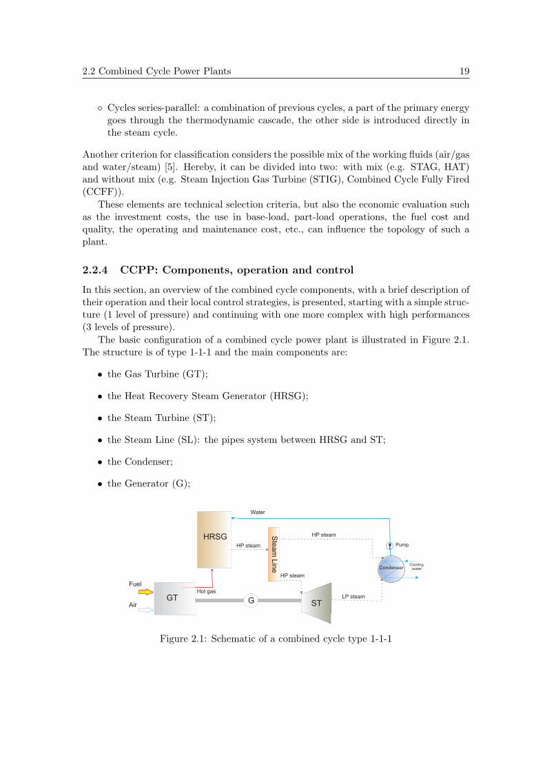
2.2 Combined Cycle Power Plants 19
⋄ Cycles series-parallel: a combination of previous cycles, a part of the primary energygoes through the thermodynamic cascade, the other side is introduced directly inthe steam cycle.
Another criterion for classification considers the possible mix of the working fluids (air/gasand water/steam) [5]. Hereby, it can be divided into two: with mix (e.g. STAG, HAT)and without mix (e.g. Steam Injection Gas Turbine (STIG), Combined Cycle Fully Fired(CCFF)).
These elements are technical selection criteria, but also the economic evaluation suchas the investment costs, the use in base-load, part-load operations, the fuel cost andquality, the operating and maintenance cost, etc., can influence the topology of such aplant.
2.2.4 CCPP: Components, operation and control
In this section, an overview of the combined cycle components, with a brief description oftheir operation and their local control strategies, is presented, starting with a simple struc-ture (1 level of pressure) and continuing with one more complex with high performances(3 levels of pressure).
The basic configuration of a combined cycle power plant is illustrated in Figure 2.1.The structure is of type 1-1-1 and the main components are:
• the Gas Turbine (GT);
• the Heat Recovery Steam Generator (HRSG);
• the Steam Turbine (ST);
• the Steam Line (SL): the pipes system between HRSG and ST;
• the Condenser;
• the Generator (G);
HRSG Ste
am
Lin
e
HP steam
HP steam
LP steam
HP steam
Water
Pump
CoolingwaterCondenser
Fuel
Air
Hot gas
G STGT
Figure 2.1: Schematic of a combined cycle type 1-1-1

20 Combined cycle power plants, start-up problem
2.2.4.1 CCPP: Single pressure level
The simplest type of combined cycle is the so called single pressure cycle (see Figure 2.1).It represents actually the basis for all possible configurations of combined cycle. In thiscycle the HRSG generates steam for ST at only one pressure level (i.e. high pressure - HP).This configuration involves a low installed cost and has been extensively used. Despitethe fact it does not provide the highest efficiency, it can be an economical solution whenthe fuel is of low quality or inexpensive, or when used during peak demand periods.
The normal operation of such a circuit is presented as follows: Ambient air is com-pressed, then mixed with fuel and burned at constant pressure. The high-temperature,high-pressure gas resulted by combustion is expanded in the GT to generate mechanicalpower. The GT exhaust hot gases are used to produce steam in the HRSG. The steamproduced is expanded in the ST to provide additional power. The exhaust steam fromthe ST is collected by a condenser. The steam cycle is completed by feeding the HRSGwith water from the condenser.
2.2.4.2 Gas Turbine
2.2.4.2.1 Description
The thermodynamic cycle which governs the behavior of GT systems, is a Brayton cycle.This cycle is one of the most efficient for the conversion of gas fuels to mechanical power[20], [18], [42].
The GT (combustion turbine) can be considered as the most important equipment ofthe combined cycle since it provides a large part of the electrical power (GT produce about60%, while ST about 40% at base load) and supplies the thermal energy needed by thesteam cycle. The three main elements which constitutes the GT are a compressor coupledto a turbine and a combustion chamber in between (Figure 2.2). Briefly their operation
Compressor Gas Turbine
Fuel
AirHot Gas
Mechanicalpower
To generator
To HRSG
Combustor
Figure 2.2: Gas turbine structure
is the following. Air at atmospheric conditions enters the compressor and is compressedto a required pressure for combustion. As a result of the adiabatic compression, the airundergoes an increase in temperature and pressure. In the combustion chamber (combus-tor), the air is mixed with fuel and burned under constant pressure conditions to convertthe fuel’s chemical energy into thermal energy. The resulting high temperature and high
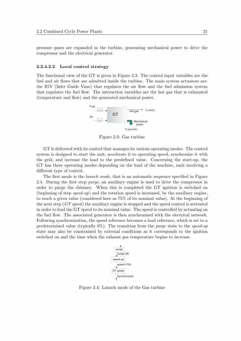
2.2 Combined Cycle Power Plants 21
pressure gases are expanded in the turbine, generating mechanical power to drive thecompressor and the electrical generator.
2.2.4.2.2 Local control strategy
The functional view of the GT is given in Figure 2.3. The control input variables are thefuel and air flows that are admitted inside the turbine. The main system actuators are:the IGV (Inlet Guide Vane) that regulates the air flow and the fuel admission systemthat regulates the fuel flow. The interaction variables are the hot gas that is exhausted(temperature and flow) and the generated mechanical power.
GT
Mechanicalpower
To HRSG
To generator
Fuel
Air
Hot gas
Figure 2.3: Gas turbine
GT is delivered with its control that manages its various operating modes. The controlsystem is designed to start the unit, accelerate it to operating speed, synchronize it withthe grid, and increase the load to the predefined value. Concerning the start-up, theGT has three operating modes depending on the load of the machine, each involving adifferent type of control.
The first mode is the launch mode, that is an automatic sequence specified in Figure2.4. During the first step purge, an auxiliary engine is used to drive the compressor inorder to purge the chimney. When this is completed the GT ignition is switched on(beginning of step speed-up) and the rotation speed is increased, by the auxiliary engine,to reach a given value (considered here as 75% of its nominal value). At the beginning ofthe next step (GT speed) the auxiliary engine is stopped and the speed control is activatedin order to lead the GT speed to its nominal value. The speed is controlled by actuating onthe fuel flow. The associated generator is then synchronized with the electrical network.Following synchronization, the speed reference becomes a load reference, which is set to apredetermined value (typically 8%). The transition from the purge state to the speed-upstate may also be constrained by external conditions as it corresponds to the ignitionswitched on and the time when the exhaust gas temperature begins to increase.
purge
GT speed
speed-up
purge OK
speed=75%
Synchronized
Figure 2.4: Launch mode of the Gas turbine
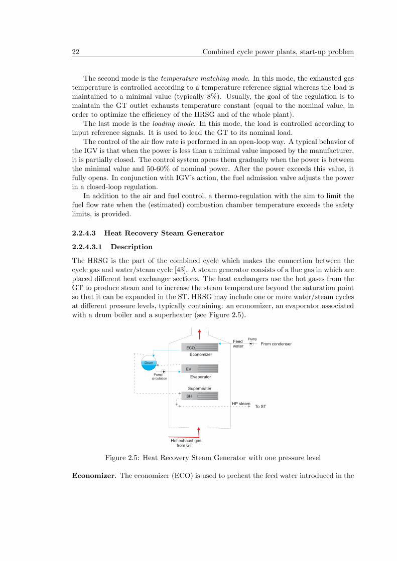
22 Combined cycle power plants, start-up problem
The second mode is the temperature matching mode. In this mode, the exhausted gastemperature is controlled according to a temperature reference signal whereas the load ismaintained to a minimal value (typically 8%). Usually, the goal of the regulation is tomaintain the GT outlet exhausts temperature constant (equal to the nominal value, inorder to optimize the efficiency of the HRSG and of the whole plant).
The last mode is the loading mode. In this mode, the load is controlled according toinput reference signals. It is used to lead the GT to its nominal load.
The control of the air flow rate is performed in an open-loop way. A typical behavior ofthe IGV is that when the power is less than a minimal value imposed by the manufacturer,it is partially closed. The control system opens them gradually when the power is betweenthe minimal value and 50-60% of nominal power. After the power exceeds this value, itfully opens. In conjunction with IGV’s action, the fuel admission valve adjusts the powerin a closed-loop regulation.
In addition to the air and fuel control, a thermo-regulation with the aim to limit thefuel flow rate when the (estimated) combustion chamber temperature exceeds the safetylimits, is provided.
2.2.4.3 Heat Recovery Steam Generator
2.2.4.3.1 Description
The HRSG is the part of the combined cycle which makes the connection between thecycle gas and water/steam cycle [43]. A steam generator consists of a flue gas in which areplaced different heat exchanger sections. The heat exchangers use the hot gases from theGT to produce steam and to increase the steam temperature beyond the saturation pointso that it can be expanded in the ST. HRSG may include one or more water/steam cyclesat different pressure levels, typically containing: an economizer, an evaporator associatedwith a drum boiler and a superheater (see Figure 2.5).
ECO
HP steam
Feedwater
From condenser
Economizer
Evaporator
Superheater
To ST
Pumpcirculation
Pump
Drum
EV
SH
Hot exhaust gasfrom GT
Figure 2.5: Heat Recovery Steam Generator with one pressure level
Economizer. The economizer (ECO) is used to preheat the feed water introduced in the

2.2 Combined Cycle Power Plants 23
drum in order to replace the steam produced and delivered. It is normally located in thecolder gas, downstream the evaporator.
Evaporator. The evaporator (EV) is designed to transform the heated liquid (water)from the drum to a saturated steam. The flow in the evaporator enters as a liquid andexits as saturated steam. The EV modules are connected to the drum via downcornerpipes, riser pipes and distribution manifolds.
Superheater. The superheater (SH) in the HRSG is used to transfer the saturated steamfrom the steam drum to a superheated steam for injection in the ST. The ”dry” processin the SH is performed at a constant pressure. In some units this steam may only beheated slightly above the saturation point while in other units it may be superheated toa significant temperature for additional energy storage. The SH is normally located inthe hotter gas stream close to the inlet of the exhaust gases from the GT.
Drum boiler. The steam drum is the connection point among economizer, evaporatorand superheater. The drum is designed to act as a storage tank as well as separator forthe saturated steam and liquid phase of water mixture. It is fed with the preheated waterfrom the economizer and the saturated steam from the evaporator.
Certainly, the improvement of the combined cycle performance is linked to the techno-logical progress of the GT and ST, but also the development in steam generators design(the increase of the recovered energy from the GT exhaust, more complex heat exchang-ers positioning, the strength of materials, etc.) plays a fundamental role [3]. Therefore,in order to maximize the energy recovery from the GT exhaust, multiple-pressure steamcycles are used.
A schematic representation of a system with three circuits - low pressure (LP), in-termediate pressure (IP) and high pressure (HP) - is given in Figure 2.6. Each circuitproduces steam at a given pressure from water. The LP section is fed with water fromthe condenser while the IP, HP sections are fed with water that has been heated by theLP circuit. In the case of the systems with reheating, the IP circuit is also fed withthe steam return from the HP exhaust ST. An informative range of the thermodynamicvalues for common configurations of HRSG is given in Table 2.1. Increasing the number
HP LPIPHot exhaust gasfrom GT
Waterfromcondenser
Feed water
Pump
Pump
Pump
HP steam Steamreturn
IP steam LP steam
Figure 2.6: HSRG decomposition
of steam pressure levels (two or three-pressure steam cycles) involves the reduction of

24 Combined cycle power plants, start-up problem
the difference between exhaust gas and steam/water energy. Mostly, the improvementof the plant performance results from additional heat transfer surface installed in theHRSG. Furthermore, in certain circumstances, the HRSG can be designed to incorporatesupplementary firing sources to improve the boiler output [19], [43].
Independent of all these configurations, an HRSG design can be of natural circulationtype (by thermosyphon principle) or forced circulation type. The type generally dependson the layout of the boiler, vertical or horizontal [44]. In a forced circulation HRSG,the steam/water mixture is circulated through evaporator tubes by using a pump. Themost common type of HRSG in combined cycle plants uses forced circulation. A completerepresentation of a HRSG with three pressure levels with reheat and forced circulationis shown in Figure 2.7. It should be also noted that the number and the position of the
ECO-LP
SH-LP
SH-IP
EV-LP
ECO-HP2
EV-HP
Feed waterFrom condenser
From HP turbine
To LP turbine
To IP turbine
FromLP drum
FromLP drum
To HP turbine
Pump
LP steam
IP steam
HP steam
Hot exhaust gasfrom GT
Steamreturn
HP Drum
ECO-HP1 ECO-IP
EV-IPIP Drum
LP Drum
DSH
MIX
SH-HP2
SH-HP1
RH-IP1
RH-IP2 DSH
Pressurecontrolvalve
Figure 2.7: HRSG with 3 pressure levels and reheat
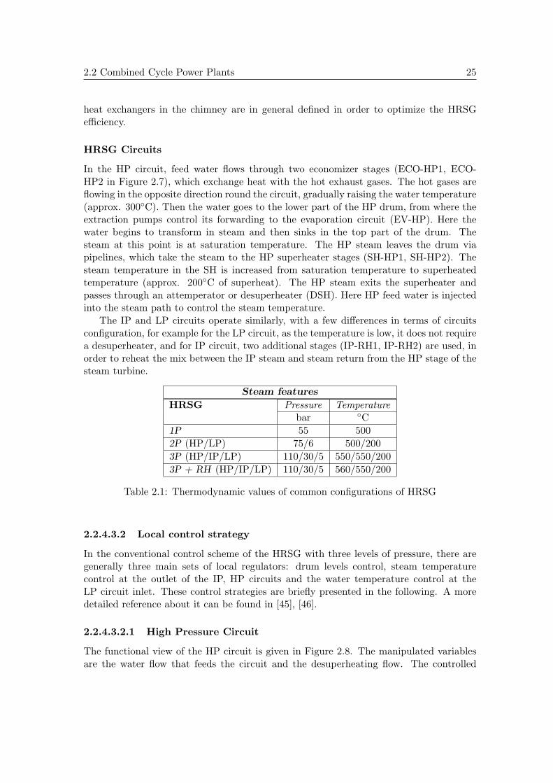
2.2 Combined Cycle Power Plants 25
heat exchangers in the chimney are in general defined in order to optimize the HRSGefficiency.
HRSG Circuits
In the HP circuit, feed water flows through two economizer stages (ECO-HP1, ECO-HP2 in Figure 2.7), which exchange heat with the hot exhaust gases. The hot gases areflowing in the opposite direction round the circuit, gradually raising the water temperature(approx. 300◦C). Then the water goes to the lower part of the HP drum, from where theextraction pumps control its forwarding to the evaporation circuit (EV-HP). Here thewater begins to transform in steam and then sinks in the top part of the drum. Thesteam at this point is at saturation temperature. The HP steam leaves the drum viapipelines, which take the steam to the HP superheater stages (SH-HP1, SH-HP2). Thesteam temperature in the SH is increased from saturation temperature to superheatedtemperature (approx. 200◦C of superheat). The HP steam exits the superheater andpasses through an attemperator or desuperheater (DSH). Here HP feed water is injectedinto the steam path to control the steam temperature.
The IP and LP circuits operate similarly, with a few differences in terms of circuitsconfiguration, for example for the LP circuit, as the temperature is low, it does not requirea desuperheater, and for IP circuit, two additional stages (IP-RH1, IP-RH2) are used, inorder to reheat the mix between the IP steam and steam return from the HP stage of thesteam turbine.
Steam features
HRSG Pressure Temperaturebar ◦C
1P 55 500
2P (HP/LP) 75/6 500/200
3P (HP/IP/LP) 110/30/5 550/550/200
3P + RH (HP/IP/LP) 110/30/5 560/550/200
Table 2.1: Thermodynamic values of common configurations of HRSG
2.2.4.3.2 Local control strategy
In the conventional control scheme of the HRSG with three levels of pressure, there aregenerally three main sets of local regulators: drum levels control, steam temperaturecontrol at the outlet of the IP, HP circuits and the water temperature control at theLP circuit inlet. These control strategies are briefly presented in the following. A moredetailed reference about it can be found in [45], [46].
2.2.4.3.2.1 High Pressure Circuit
The functional view of the HP circuit is given in Figure 2.8. The manipulated variablesare the water flow that feeds the circuit and the desuperheating flow. The controlled

26 Combined cycle power plants, start-up problem
variables are the HP drum level and the output steam temperature (HP steam) that isdirected through pipes to the ST. In this circuit, the circulation pump is used to assurea constant flow in the evaporator. In certain cases, the circulation in the evaporator isdone without pump by natural thermosyphon phenomenon.
The drum level is controlled according to an input reference signal by actuating afeedwater valve/pump. The position of this valve can vary as a function of the variousdesigns of the HRSG manufacturers (e.g. upstream or downstream of the economizer).The regulation of the HP steam temperature is performed according to a temperaturereference signal by desuperheating the corresponding steam fluxes, i.e. by injecting waterupstream the inlet section of the superheater (SH).
Drum HP
EV
ECO
SH
Water
HP Steam
from LP circuit
Controlvalve/pump
to HP turbine
Water fromLP circuit
Desuperheater
Figure 2.8: HP circuit
2.2.4.3.2.2 Intermediate Pressure Circuit
The control strategy is the same, the IP drum level is controlled according to an input level
Drum IP
EV
ECO
SH
Water
Water fromLP circuit
IP Steam
Pressurecontrolvalve
Steamreturn
from HP turbine
from LP circuit
to IP turbine
Desuperheater
RH
MIX
Controlvalve/pump
Figure 2.9: IP circuit
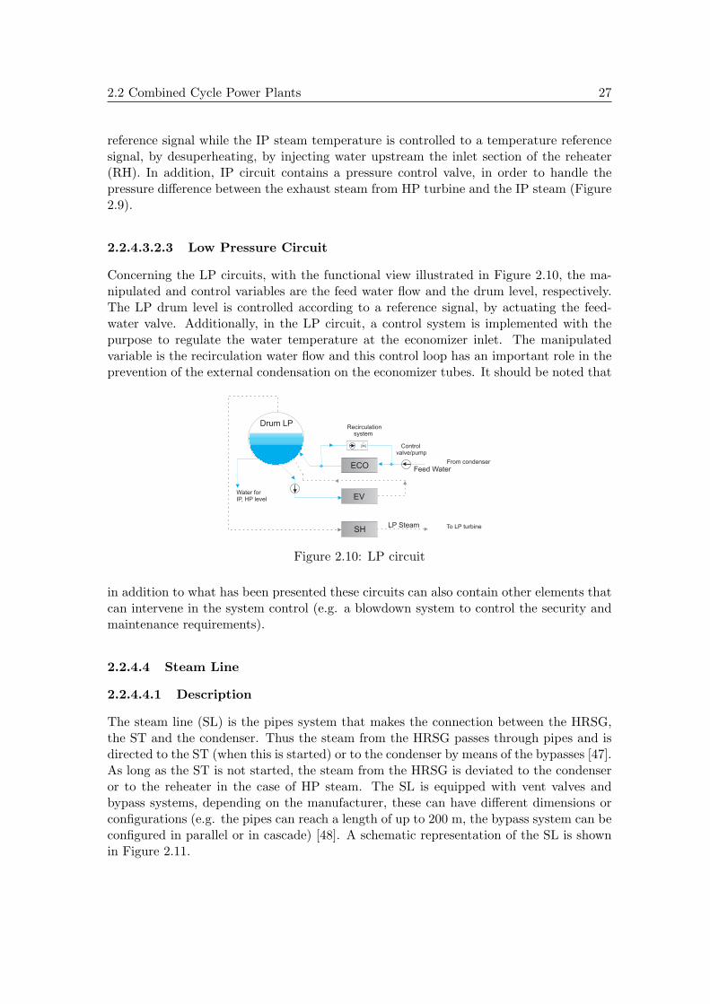
2.2 Combined Cycle Power Plants 27
reference signal while the IP steam temperature is controlled to a temperature referencesignal, by desuperheating, by injecting water upstream the inlet section of the reheater(RH). In addition, IP circuit contains a pressure control valve, in order to handle thepressure difference between the exhaust steam from HP turbine and the IP steam (Figure2.9).
2.2.4.3.2.3 Low Pressure Circuit
Concerning the LP circuits, with the functional view illustrated in Figure 2.10, the ma-nipulated and control variables are the feed water flow and the drum level, respectively.The LP drum level is controlled according to a reference signal, by actuating the feed-water valve. Additionally, in the LP circuit, a control system is implemented with thepurpose to regulate the water temperature at the economizer inlet. The manipulatedvariable is the recirculation water flow and this control loop has an important role in theprevention of the external condensation on the economizer tubes. It should be noted that
Drum LP
EV
ECO
SH
Feed Water
Controlvalve/pump
Recirculationsystem
Water forIP, HP level
From condenser
To LP turbineLP Steam
Figure 2.10: LP circuit
in addition to what has been presented these circuits can also contain other elements thatcan intervene in the system control (e.g. a blowdown system to control the security andmaintenance requirements).
2.2.4.4 Steam Line
2.2.4.4.1 Description
The steam line (SL) is the pipes system that makes the connection between the HRSG,the ST and the condenser. Thus the steam from the HRSG passes through pipes and isdirected to the ST (when this is started) or to the condenser by means of the bypasses [47].As long as the ST is not started, the steam from the HRSG is deviated to the condenseror to the reheater in the case of HP steam. The SL is equipped with vent valves andbypass systems, depending on the manufacturer, these can have different dimensions orconfigurations (e.g. the pipes can reach a length of up to 200 m, the bypass system can beconfigured in parallel or in cascade) [48]. A schematic representation of the SL is shownin Figure 2.11.

28 Combined cycle power plants, start-up problem
HP steamfrom HRSG
HP steam
IP steamfrom HRSG
IP steam
IP steam
LP steamfrom HRSG
LP steam
LP steam
Steam returnto HRSG
Steamreturn
Bypass
Bypass
Bypass
To the Condenser
To Condenser
To LP turbine stage
To IP turbine stage
To HP turbine stage
From HP turbine stage
Steam Line
Vent valve
Vent valve
Vent valve
Vent valve
Vent valve
Vent valve
Figure 2.11: SL schematic representation
2.2.4.4.2 Local control strategy
In general, the SL’s control role in a combined cycle plant is mainly related to the start-upphase. Its objective is to avoid the sudden warming of the pipes (to limit the thermalshocks and to avoid the condensation). Also the main steam entering the ST has tofulfill certain conditions such as temperature, pressure and quality, necessary for thesafe operation of the ST. These conditions are reached by controlling the steam that isadmitted inside the pipe with the evacuation and the bypass systems.
The bypass system is used also during the start-up phase to control the steam pressure.Thereby, a control system throttles the bypass valves, in order to maintain the pressurein the circuits at the set points and to ensure that it does not reach the safety limits.
2.2.4.5 Steam Turbine
2.2.4.5.1 Description
The ST operates on the Rankine cycle using the high-enthalpy (high pressure and temper-ature) steam provided by HRSG to generate mechanical power. In this thermodynamiccycle the working fluid follows a closed loop and is constantly reused, unlike the Braytoncycle that usually works as an open system. The steam turbine converts the thermalenergy in the steam into mechanical energy. A turbine contains several sets of blades(buckets): a set of stationary blades (nozzles) which is connected to the casing and a setof rotating blades which is connected to the shaft. The stationary blades convert storedenergy of high temperature and high pressure steam into kinetic energy (velocity) anddirect the flow onto the rotating blades. The rotating blades transform the kinetic energyin impulse and reaction forces caused by pressure drop, which results in the rotation ofthe turbine rotor (rotor mounted on turbine shaft) [18].
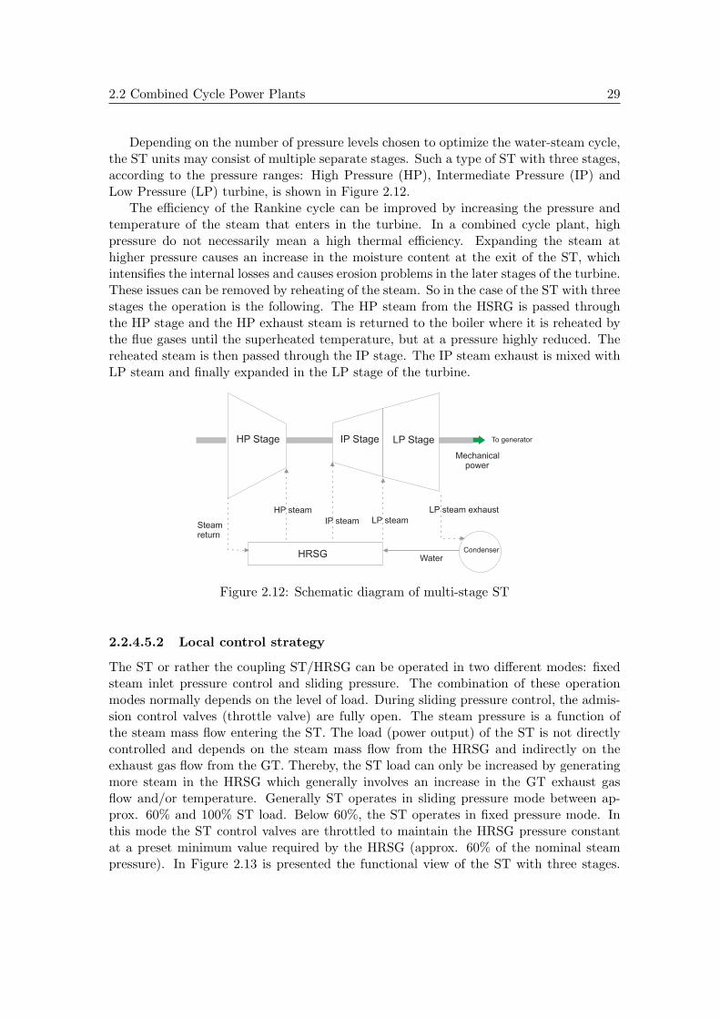
2.2 Combined Cycle Power Plants 29
Depending on the number of pressure levels chosen to optimize the water-steam cycle,the ST units may consist of multiple separate stages. Such a type of ST with three stages,according to the pressure ranges: High Pressure (HP), Intermediate Pressure (IP) andLow Pressure (LP) turbine, is shown in Figure 2.12.
The efficiency of the Rankine cycle can be improved by increasing the pressure andtemperature of the steam that enters in the turbine. In a combined cycle plant, highpressure do not necessarily mean a high thermal efficiency. Expanding the steam athigher pressure causes an increase in the moisture content at the exit of the ST, whichintensifies the internal losses and causes erosion problems in the later stages of the turbine.These issues can be removed by reheating of the steam. So in the case of the ST with threestages the operation is the following. The HP steam from the HSRG is passed throughthe HP stage and the HP exhaust steam is returned to the boiler where it is reheated bythe flue gases until the superheated temperature, but at a pressure highly reduced. Thereheated steam is then passed through the IP stage. The IP steam exhaust is mixed withLP steam and finally expanded in the LP stage of the turbine.
HP Stage
HRSG
IP Stage
HP steam
IP steam LP steam
To generator
Mechanicalpower
LP steam exhaust
Steamreturn
WaterCondenser
LP Stage
Figure 2.12: Schematic diagram of multi-stage ST
2.2.4.5.2 Local control strategy
The ST or rather the coupling ST/HRSG can be operated in two different modes: fixedsteam inlet pressure control and sliding pressure. The combination of these operationmodes normally depends on the level of load. During sliding pressure control, the admis-sion control valves (throttle valve) are fully open. The steam pressure is a function ofthe steam mass flow entering the ST. The load (power output) of the ST is not directlycontrolled and depends on the steam mass flow from the HRSG and indirectly on theexhaust gas flow from the GT. Thereby, the ST load can only be increased by generatingmore steam in the HRSG which generally involves an increase in the GT exhaust gasflow and/or temperature. Generally ST operates in sliding pressure mode between ap-prox. 60% and 100% ST load. Below 60%, the ST operates in fixed pressure mode. Inthis mode the ST control valves are throttled to maintain the HRSG pressure constantat a preset minimum value required by the HRSG (approx. 60% of the nominal steampressure). In Figure 2.13 is presented the functional view of the ST with three stages.

30 Combined cycle power plants, start-up problem
ST
Mechanicalpower
HP steam
IP steam
Steamreturn
LP steam
LP steamTo condenser
To generator
FromHRSG
ToHRSG
ST control valve
Figure 2.13: Steam Turbine
In the fixed inlet pressure control mode, the valves allow to control the steam admission(HP, IP, LP steam) inside the ST stages. During the start-up sequence, controlling thesteam flow, by actuating on the throttle valves, the ST rises gradually in speed and intemperature. The ST accepts the total HRSG steam flow (sliding pressure mode), whenthe bypass is closed.
2.2.4.6 Condenser
2.2.4.6.1 Description
The condenser is the device that converts the steam exiting from the ST in water. Oncethe steam has passed through the ST, it is taken by the condenser, which removes theheat until it condenses back into liquid water. This is done by passing the wet steamaround several cold water tubes. The condensed steam is collected at the bottom of thecondenser and returned to the HRSG using extraction pumps, to continue the water-to-steam cycle. The condenser operates usually at very low vacuum pressures of about 0.1bar.
2.2.4.6.2 Local control strategy
In the case of the condenser the local regulators aim: the level, the inlet steam temperatureand the vacuum pressure. The functional view of the condenser is given in Figure 2.14.The manipulated variables are the water flow, the desuperheating flow and the vacuumflow. The condenser level is controlled according to a reference signal, controlling the water
Condenser
Water
IP steam
LP steam
Coolingwater
HP steam
Water
Vacuum
DSH
From ST
FromHRSG
Water
Water
To HRSG
Figure 2.14: Condenser
2.2 Combined Cycle Power Plants 31
inflow, i.e. by actuating on the water pump. The regulation of the steam temperatureis performed according to a set point signal by desuperheating the corresponding steamfluxes, i.e. by injecting water upstream the inlet section of the condenser. Normally,this regulation is active at start-up when the bypasses are used. The vacuum pressure iscontrolled by actuating the vacuum pump, according to a reference signal.
2.2.4.7 GT and ST electrical generators
The generator is used to convert the rotating mechanical energy of the GT or ST intoelectrical energy. The turbine and generator rotors are connected through a coupling.The rotation of the turbine blades causes the rotation of the generator rotor shaft. So,the generator converts the rotating mechanical energy transmitted to it into electricalenergy.
In a large part of the CCPPs, the GT and the ST have separate generators, using amulti-shaft configuration. In Europe, a popular option is to use a single shaft arrangement.In this design the GT and ST are on the same shaft using only one generator (see forexample Figure 2.1). This configuration represents the economic option, offering a loweroverall cost.
2.2.4.8 CCPP: Multi-pressure levels
Summarizing what has been presented so far, the multiple-pressure steam cycles are forthe most part similar to the single pressure cycle, with the addition of the LP and IPsections, in the HRSG. In this case, the difference in operation is the following. TheGT exhaust gas is used to produce steam at different levels of pressure. This steam isexpanded sequentially in the ST stages to obtain additional power. In addition concerningthe systems which provide a sufficient high thermal energy to reheat the steam, the HPexhaust steam from the ST is mixed with IP steam and reheated in the HRSG to captureadditional energy from the exhaust gases, before the expansion in the IP turbine stage.The steam from the IP turbine exhaust is mixed with LP steam from the HRSG LPcircuit and then expanded in the LP steam turbine up to the condenser pressure. Thesteam cycle is completed by feeding the three circuits in the HRSG with the water fromthe condenser to the LP drum and then from the LP drum to the IP and HP drums.
Multi-pressure steam generation achieves a better efficiency than a single pressuresystem but with a higher investment costs. In general, the plants with multi-pressurecircuits are the economic option if the fuel price is high or if the duty cycle requires ahigh plant load factor. This type of system represents the most efficient power plantcurrently available. A simplified representation of such a CCPP, without any auxiliarysystem and with the main sensors and actuators, is presented in Figure 2.15.

32Com
bined
cycle
pow
erplan
ts,start-u
pprob
lem
HP IP LP
Vent valve
Pump
Spray valveVent valve
Watersource
Watersource
Watersource
Watersource
Condenser
WaterPump
Water
Coolingwater
DSH
DSH
ECO-LP
SH-LP
RH-IP1
SH-IP
EV-LP
ECO-HP2
ECO-HP3
ECO-HP4
SH-HP1
SH-HP2
SH-HP3
RH-IP2
EV-IP
Hot gas
EV-HP
LP steam
IP steam
HP steam
ATT-SH
ATT-RH
MIX
IP Drum
HP Drum
TT
TT
TT
LT
TT
TTTT
TT
LT
LT
PT
PT
LT
TT
PT
PT
PT
PT
PT
PT
SpTSpT
PT
PT
LP Drum
ECO-HP1 ECO-IP
GGGT
Fuel
Air
Valve IP
AdmissionValve
AdmissionValve
BypassLP
Bypass
IP
Bypass
HP
LdT
LdT
Figure 2.15: CCPP with 3P RH
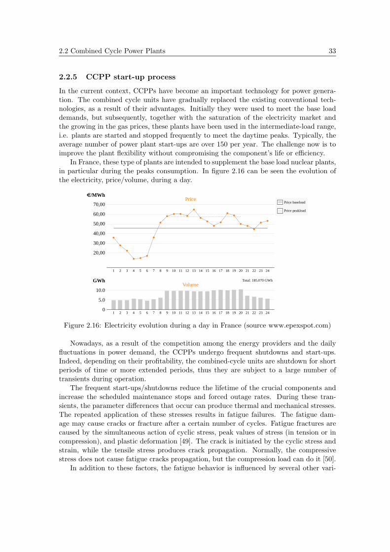
2.2 Combined Cycle Power Plants 33
2.2.5 CCPP start-up process
In the current context, CCPPs have become an important technology for power genera-tion. The combined cycle units have gradually replaced the existing conventional tech-nologies, as a result of their advantages. Initially they were used to meet the base loaddemands, but subsequently, together with the saturation of the electricity market andthe growing in the gas prices, these plants have been used in the intermediate-load range,i.e. plants are started and stopped frequently to meet the daytime peaks. Typically, theaverage number of power plant start-ups are over 150 per year. The challenge now is toimprove the plant flexibility without compromising the component’s life or efficiency.
In France, these type of plants are intended to supplement the base load nuclear plants,in particular during the peaks consumption. In figure 2.16 can be seen the evolution ofthe electricity, price/volume, during a day.
1 2 3 4 5 6 7 8 9 10 11 12 13 14 15 16 17 18 19 20 21 22 23 24
20,00
30,00
40,00
50,00
60,00
70,00
e/MWh
Total: 185.070 GWh
Price baseload
Price peakload
Price
1 2 3 4 5 6 7 8 9 10 11 12 13 14 15 16 17 18 19 20 21 22 23 24
Volume
0
5.0
10.0
GWh
Figure 2.16: Electricity evolution during a day in France (source www.epexspot.com)
Nowadays, as a result of the competition among the energy providers and the dailyfluctuations in power demand, the CCPPs undergo frequent shutdowns and start-ups.Indeed, depending on their profitability, the combined-cycle units are shutdown for shortperiods of time or more extended periods, thus they are subject to a large number oftransients during operation.
The frequent start-ups/shutdowns reduce the lifetime of the crucial components andincrease the scheduled maintenance stops and forced outage rates. During these tran-sients, the parameter differences that occur can produce thermal and mechanical stresses.The repeated application of these stresses results in fatigue failures. The fatigue dam-age may cause cracks or fracture after a certain number of cycles. Fatigue fractures arecaused by the simultaneous action of cyclic stress, peak values of stress (in tension or incompression), and plastic deformation [49]. The crack is initiated by the cyclic stress andstrain, while the tensile stress produces crack propagation. Normally, the compressivestress does not cause fatigue cracks propagation, but the compression load can do it [50].
In addition to these factors, the fatigue behavior is influenced by several other vari-
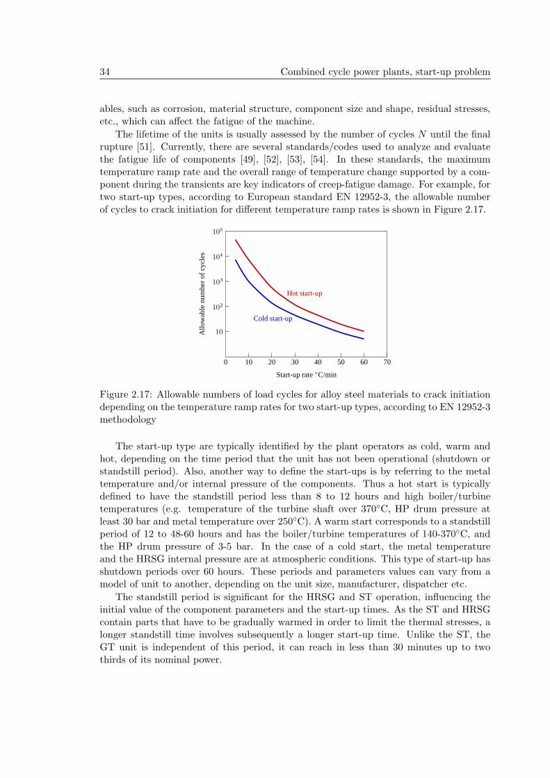
34 Combined cycle power plants, start-up problem
ables, such as corrosion, material structure, component size and shape, residual stresses,etc., which can affect the fatigue of the machine.
The lifetime of the units is usually assessed by the number of cycles N until the finalrupture [51]. Currently, there are several standards/codes used to analyze and evaluatethe fatigue life of components [49], [52], [53], [54]. In these standards, the maximumtemperature ramp rate and the overall range of temperature change supported by a com-ponent during the transients are key indicators of creep-fatigue damage. For example, fortwo start-up types, according to European standard EN 12952-3, the allowable numberof cycles to crack initiation for different temperature ramp rates is shown in Figure 2.17.
0 10 20 30 40 50 60 70
Start-up rate ◦C/min
10
102
103
104
105
Allo
wab
lenu
mbe
rof
cycl
es
Hot start-up
Cold start-up
Figure 2.17: Allowable numbers of load cycles for alloy steel materials to crack initiationdepending on the temperature ramp rates for two start-up types, according to EN 12952-3methodology
The start-up type are typically identified by the plant operators as cold, warm andhot, depending on the time period that the unit has not been operational (shutdown orstandstill period). Also, another way to define the start-ups is by referring to the metaltemperature and/or internal pressure of the components. Thus a hot start is typicallydefined to have the standstill period less than 8 to 12 hours and high boiler/turbinetemperatures (e.g. temperature of the turbine shaft over 370◦C, HP drum pressure atleast 30 bar and metal temperature over 250◦C). A warm start corresponds to a standstillperiod of 12 to 48-60 hours and has the boiler/turbine temperatures of 140-370◦C, andthe HP drum pressure of 3-5 bar. In the case of a cold start, the metal temperatureand the HRSG internal pressure are at atmospheric conditions. This type of start-up hasshutdown periods over 60 hours. These periods and parameters values can vary from amodel of unit to another, depending on the unit size, manufacturer, dispatcher etc.
The standstill period is significant for the HRSG and ST operation, influencing theinitial value of the component parameters and the start-up times. As the ST and HRSGcontain parts that have to be gradually warmed in order to limit the thermal stresses, alonger standstill time involves subsequently a longer start-up time. Unlike the ST, theGT unit is independent of this period, it can reach in less than 30 minutes up to twothirds of its nominal power.
2.2 Combined Cycle Power Plants 35
The cycling operations, in particular the start-up, can be quite damaging for the powergeneration equipment. The main concern in CCPP start-ups is to avoid the phenomena(e.g. thermal stress, mechanical stress) that may shorten the component’s life and pro-duce unsafe situations. All this consideration results in the start-up time increasing, whileeconomical requirements are to reduce this time and to minimize the operation costs. Cur-rently, in order to prevent any possible unsafe conditions and to preserve the componentslife, a number of physical constraints has been introduced. In the following section, themain constraints related to the start-up phase as well as the physical limitations of thesystems, are mainly outlined.
2.2.5.1 GT: Physical limitations and constraints
Generally, the GT is not a limiting factor for the CCPP start-up time, since the GT start-up is much faster than the HRSG/ST system start-up time. Also during transients, theGT has a dynamic response (seconds) faster than the HRSG/ST assemblage (minutes).The GT’s control system performs the start-up and ensures a progressive increase of theturbine rotor temperature. The system disposes also of protection circuits [18], to ensuresafety operation of all the GT’s subsystems and prevent abnormal situations, which couldlead to the plant shutdown:
• overspeed: when the speed exceeds the security limit (typically 110%);
• overtemperature: when the average exhaust temperature exceeds the set limit point;
• overloading: when the load of the turbine is too high with respect to its nominalvalue;
• loss of flame: when fuel/air ratio exceeds the flame extinction limit.
In addition, during start-up phase, a number of constraints are imposed on the GT’sparameters. These constraints are rather a consequence of the fact that the HRSG/STsystem is not able to support a sudden change in steam characteristics (temperature,pressure) and quantity. For a large GT load increase (e.g. more than 5%), in order toguarantee the safety and the availability of the operations, it is necessary to limit theGT load change. In general the load increase is limited to a rate of about 2% -5%/min.Thus, depending on the operating mode, the constraints are specified on the gradientsof the gas temperature or the load. The constraint on temperature gradient is mainlyconsidered during the temperature matching mode, whereas the one on the load gradientis considered during the loading mode.
2.2.5.2 HRSG: Physical limitations and constraints
The physical limitations and constraints related to the HRSG circuits are mainly linkedto the component life consumption, in particular to the stress of the material. As thepressure and temperature are higher, these constraints are more critical for the HP andIP circuits.
36 Combined cycle power plants, start-up problem
2.2.5.2.1 High Pressure and Intermediate Pressure Circuits
A first type of constraints is related to stress on certain components. The componentsin the HRSG which have been identified as critical, in terms of fatigue damage, are theoutlet headers of the reheater and HP superheater, the parts of the exchanger located inthe hotter gas stream, and to a lesser extent, the thick boiler drums walls. The two maintypes of stress on the components surface, which can occur, are: the mechanical stressresulting from internal pressure and the thermal stress resulting from thermal expansion.Thus the constraints are mainly specified on the pressure and temperature gradients.
Considering the fact that condensation is an important phenomenon that occurs dur-ing the start-up in SL downstream and that can be damaging for the components withthick metallic parts, such as the superheater headers, constraints on the quantity ofcondensation are imposed. This phenomenon occurs when the steam of the drum cancondense in the superheater section, therefore it is necessary to limit the condensate for-mation in the colder part of the SH and to prevent slugs of condensate to be pushed intothe steam pipes by an efficient control of the evacuation system (vent and drain valves).
Also, another type of constraints is specified on the minimum flow rate in pumps,in the case of the plants with forced circulation. This constraint is imposed to avoidthe cavitation in pumps [42]. This phenomenon degrades the performance of the pump,resulting in fluctuating flow rate, discharge pressure and in some cases even to the pumpcomponents destruction. In general this constraint is imposed on all circuits equippedwith a pump.
2.2.5.2.2 Low Pressure Circuit
The LP circuit works at low temperature, so in terms of thermal stress, it is not critical.In this case, in order to keep the mechanical stress in the allowable limits, the constraintsare specified on the gradient of pressure in the LP drum.
In addition, at this level a constraint, that aims the temperature of the flue gas, isspecified. It is important to maintain the gas temperature above the acid gas dew point,because the gas condensation can occur, causing serious corrosion problems for the metal-lic parts in contact with these gases.
The values of the gradients used to prevent the fatigue failures, are typically determinedin accordance with international standards and codes (see [49], [53], [54]). As mentionedbefore, the most critical components in the HRSG circuit are the drums and high tem-perature superheater/reheater headers. For each of them a number of precise limits areestablished, thus for large steam drums with a wall thickness greater than 100 mm, oper-ating at 100 bar and over, the acceptable temperature gradient is generally of 36◦C/min,while for smaller drums operating at 60 bar, the temperature gradient can be up to8◦C/min. For the superheaters depending on the wall thickness, the acceptable tempera-ture gradient can reach up to 17◦C/min (e.g. for a SH with a wall thickness greater than25 mm, the acceptable temperature gradient is of 17◦C/min) [46].
The main protection limits for the HRSG (for all circuits HP, IP, LP) are:
• overtemperature: when the steam temperature exceeds the safety limit;

2.2 Combined Cycle Power Plants 37
• high drum level: when the level is too high, the drum can give wet steam, leadingto turbine blade erosion;
• low drum level (loss of water): when the boiler has a loss of feed water, this canboil dry, leading to a dangerous situation. For example, if in the empty boiler feedwater is injected, the water instantaneously boils on contact with the superheatedmetal and leads to explosion;
• low water pressure in desuperheater: when the water pressure injected is too low;
• feed water flow deviation: when the flow exceeds the maximum capability of thefeed water system;
• overpressure: when the pressure in tubes increases over the safety limit.
2.2.5.3 SL: Physical limitations and constraints
Concerning the SL, the main concern is also to limit the components lifetime consump-tion. Thus, a first type of constraints refers to the gradients of increasing pressure andtemperature in pipes.
The second type of constraints aims the condensation. The condensate formation andmigration through pipes must be avoided, otherwise, as mentioned above, harmful effectson the plant components can occur.
In some cases, the purge flow rate is too low and a part of condensate can not beblown off. Hence, to ensure that the condensation effect is eliminated, constraints arespecified on the purge flow rate.
For safe operation, the system is equipped with protection circuits to avoid the fol-lowing situations:
• overpressure: when the pressure in pipes exceeds the security limit;
• high condensate level: when the condensate level is too high (flooding).
2.2.5.4 ST: Physical limitations and constraints
It is generally known that during the start-up operations the ST’s life is the most affected.As previously pointed out, the main factors for the lifetime consumption and thus themain limitations for the reduction of the start-up time are derived from the temperaturegradients which occur in the components with thickest metallic parts. For the ST, theseparts are the HP/IP rotors and casings [55]. The most critical constraint is localized inthe ST rotor [56], more exactly the part of turbine shaft located close to the admission,where the temperature variations are faster and more intense (temperature increasesquickly from about 90◦C to 570◦C during start-ups). The rotor represents the componentwith the highest cost and requires a long outage to be replaced. The large temperaturevariations to which the rotor is subject produce two potential side effects: the developmentof thermal stresses and the differential expansion between stationary and rotating parts.Both phenomena can cause fatigue damage and reduce the life-time of the turbine ifthey are not properly handled. Namely, the high thermal stresses reduce the life-time

38 Combined cycle power plants, start-up problem
of the rotor, by favoring the cracks apparition, cracks propagation, and even fractures.Also, a large differential expansion can give rise to rubbing, which in turn may lead topermanent deformation (creep) and turbine performance degradation. In general, thecreep phenomenon depends much on the stress temporal peak while the fatigue crack iscaused by the repeated application of stress.
In addition to the thermal stress, the start-up rotor stress, which is directly related tothe ST’s life, contains the mechanical stress produced by centrifugal force caused by therotation speed, and in certain cases the electrically induced stress which occurs due to afaulty synchronization or a short circuit.
Acceleration of the ST start up leads in general to stress increase (mechanical, ther-mal) in their components [55]. In most cases the limitation of the stress is performed byimposing several constraints on: the gradient of increasing steam temperature at admis-sion, the gradient of speed/load, the difference between metal and steam temperatures aswell as on the temperature difference between the static and rotating parts.
Many units experienced corrosion and erosion problems. The imposed constraintsto avoid these problems are on the moisture content of steam and the level of waterpurification. The ST must be started with dry steam, if the moisture content of thesteam is over a predefined limit (typically 10% moisture content), major erosion andcorrosion problems can occur. In general the steam is superheated and no moisture ispresent at the inlet. However, moisture can appear at the outlet, particularly for the LPstage. Concerning the water purification, any admission into ST is not possible while thesteam does not have the required purity (below 0.03%).
In some cases the constraints are specified on the steam exhaust from LP stage. Thepressure of the steam which goes out of the turbine has to be limited, in order to reducethe mechanical stress.
Concerning the abnormal situations and safety operation, which could lead to a pro-cedural execution failure (turbine trip), the system provides protection circuits duringseveral events:
• overspeed: when the rotating speed of the turbine is too high; that can occur whenthe torque generated by the steam flow exceeds the countertorque generated by theload;
• high HP exhaust steam temperature: when the HP turbine exhaust steam temper-ature (steam return) is too high;
• water ingress to blade: when the moisture content of steam is over the safety limit(a limit is set at about 90% steam quality);
• low HP turbine pressure: when the pressure is too low;
• high bearing temperature: when the temperature inside the turbine is too high;
• high turbine exhaust pressure (low condenser vacuum): when the turbine exhaustpressure is high, the last stage of the blades in the low-pressure (LP) turbine willbecome overheated and damaged;

2.2 Combined Cycle Power Plants 39
• etc.
In the last decades the effects of the thermal transients on the component life have beencontinuously studied and a number of precise limits on the stresses have been imposed inorder to ensure a safety plant operation [57], [58], [55]. These limits specify the allowablestress levels in the critical components and represent the main operating constraints whichare considered in the start-up optimization procedure presented in the following sections.
2.2.5.5 Condenser: Physical limitations and constraints
The condenser usually does not have particular constraints, the safe operation is ensuredby protection circuits which avoid situations such as:
• high condenser pressure: when the pressure in condenser exceeds the security limits;
• high condenser temperature: when the temperature exceeds the safety limits;
• water level: when level of liquid water in condenser exceeds the allowable limits(level too high/low).
2.2.5.6 Start-up sequence
CCPP start-up is a complex task including several phases and conditions that must berespected simultaneously. The start-up procedure depends on each technology employed,but in general it can be decomposed into four main stages1 (Figure 2.18) that correspondto different objectives and active constraints [42]:
1. Preparation phase: this first stage prepares the ignition of the GT;
2. HRSG Start-up phase: this phase corresponds to the thermal conditioning, andits aim is to start the HRSG in order to obtain the characteristics of the steam(temperature, pressure, quality) suitable to the admission in the ST;
3. ST Start-up phase: during this stage the ST is started by admitting steam;
4. Increasing Load phase: during the last stage the load of the plant is increased toits expected level.
The CCPP start-up sequence that has been considered in this work begins when theGT is started and finishes when the plant achieves a preset level of power output2, closeto the nominal value. In fact, several conditions are required before the GT start, such asthe cooling system, extraction and feedwater pumps circuits started, etc. These actionsare supposed to be done. The overall sequence description can be found in [46].
1In some cases, the process of start-up can be modified to cope with the different environmentalrequirements dictated by local regulations
2This value can vary from one manufacturer to another

40 Combined cycle power plants, start-up problem
Steam/metalconditions
PreparationPreparation
Ignition
GT HRSG
Synchronized
Temperaturematching
Acceleration Warming
Temperaturecondtions
Pressurization
GT HRSG
Synchronized
Temperaturematching
Acceleration
GT ST
ST
ST
HRSG
LoadControl
HRSG/STconnected
HRSG on ST
HRSG Ready
Loading
FullLoad
GT STHRSG4
3
2
Off
Off
1
Figure 2.18: Start-up process decomposition
2.2.5.6.1 Preparation phase
During this stage, the GT is started by an external device, and the plant is purged toensure a non-flammable atmosphere in the turbine and HRSG, prior to ignition. Purging isusually carried out by speeding-up and holding the gas turbine at ignition speed (approx.25-30% of nominal speed) with an engine or a similar starting equipment, until a specifiednumber of air changes occurs in the GT/HRSG system.
During the purge, the exhaust from the GT is close to ambient temperature and byentering into a hot HRSG will produce a cool off in the entire boiler. In some cases (i.e.warm/hot start-up), the condensate can occur in superheater section. Once it formed, thecondensate must be removed to prevent slugs of condensate to be pushed into the systempipes (condensate migration). During this phase, the drums level control is activated tomitigate the swell effect that can appear when the GT is fired and kept active until theend of the start-up sequence. A first constraint that the control system has to respect ison the feed water flow (minimum flow rate). When the purge is completed and the levelin drums reaches the reference value, this stage is finished by firing the GT.
2.2.5.6.2 HRSG Start-up phase
The second stage begins with the GT ignition. The GT is then accelerated and syn-chronized to the grid. After synchronization the GT switches to temperature matchingmode and the exhaust gas temperature is controlled to gradually warm up the HRSGmetal (Warming mode). When the metal temperature of the HRSG (mainly of the su-perheater) is higher than the saturated steam temperature (temperature conditions), theHRSG goes to the pressurization phase.

2.2 Combined Cycle Power Plants 41
In order to avoid condensate formation and obtain characteristics of the steam (tem-perature, pressure, quality) necessary to ST start-up while warming the SL, the pressurecontrol (via bypasses and vent system) and steam temperature regulation (output HP, IPcircuits, via desuperheating) are started. With the HRSG start-up phase, the constraintsrelated to this system become active (e.g. the gradients of increasing temperature in SHs,the gradient of increasing pressure in drums, the condensate level in the SL, etc.).
When the steam conditions (pressure, temperature, quality) for ST start-up are ful-filled, the steam is directed to ST and system goes to the third phase. For the entire timeperiod until the fulfillment of the steam conditions, the generated steam is dischargedthrough the bypass into either the condenser and reheat steam line or only into the con-denser, depending on the configuration. In general the steam conditions depend on theinitial temperature inside the IP stage of the ST.
2.2.5.6.3 ST Start-up phase
During this stage, the GT is kept on temperature matching mode and the HRSG is readyto start the ST. The control of the parameters already activated (i.e. gas temperature,steam pressure, steam temperature and drum level) is maintained. By actuating on thethrottle valve opening, the steam is gradually admitted in the ST, that is started, thenaccelerated and synchronized to the electrical power grid. The ST starts with steamadmission in the IP stage and when the HP steam reaches the required temperaturelimit, it is admitted in the HP stage. After synchronization the ST begins to load (fixedsteam inlet pressure control mode), tracking a pressure set point imposed by the HRSG.
In conjunction with ST Start-up phase, the system control has to respect also theconstraints concerning the ST operation (e.g. the gradient of speed, the gradient ofincreasing temperature, the gradient of increasing load, the steam quality, etc.).
The system goes to the next phase when the connection between the HRSG and theST is complete (the bypasses are closed and the ST synchronized to the grid).
2.2.5.6.4 Increasing Load phase
In this phase, the bypass systems are closed and the entire amount of steam producedin HRSG is taken by ST (HRSG on ST mode). The GT load is controlled in order toachieve the full load (Loading mode). The ST follows the GT, increasing steam production,and switches from the fixed pressure mode to the sliding pressure mode. The start-upprocedure is finished when the power plant work at full power. In the case when theCCPP has two GTs, the second GT starts up when the ST loads.
During start-up, in addition to the active constraints for each phase, the system controlhas to guarantee the safety of the operations.
2.2.5.7 Objectives of start-up optimization
The optimization of the start-up can aim several purposes. The ideal solution should allowthe plant operator to reach the following objectives, while respecting the constraints.
42 Combined cycle power plants, start-up problem
2.2.5.7.1 Minimization of start-up time
A shorter start-up time represents the most important goal because it may be followedby other benefits presented below as targets. It can improve the operational efficiency,reducing the fuel consumption and consequently the CO2 emissions. Also, minimizingthe start-up time is a crucial competitive advantage in a liberalized market since it isdesirable to propose the smallest starting time among all energy providers
2.2.5.7.2 Minimization of the operating costs
Start-up costs include costs for fuel or other consumables such as water and chemicals.A reduction of these consumables means a direct increase of the customer value.
2.2.5.7.3 Minimization of material wear
This minimization has generally two main benefits:
• to reduce the plant life-time consumption;
• to reduce the number of maintenance stops.
2.2.5.7.4 Minimization of environmental impacts
The reduction of pollutant emissions has a major importance in view of the constantlyincreasing restrictions on the environmental impact by law. The high temperature inthe combustion zone (exceeding 1300◦C) results in the nitrogen in the air combining withoxygen, also additional nitrogen could be present in the fuel; consequently the combustiontemperature and the NOx concentrations have to be limited.
2.2.5.7.5 Minimization of start-up failure
This represents also an important point since a missed start means time lost and thesystem impossibility to respond to the dispatching request. This goal can not be easilyassociated with a criterion as previously case. To minimize the risk of start-up failure, ananalysis must be done to determine the main causes (model error, sensor error, etc.) andto choose a criterion that increases the robustness of the control with respect to thesecauses.
Generally these objectives should be considered all together and not separately; it isobvious that by considering the plant life as the first priority (e.g. minimization of thematerial wear) will result in a relatively long start-up time. On the other hand, foreconomic reasons, the start-up procedure should be achieved in the shortest time with aminimum operating cost. For that, a compromise between a fast start-up and the otherobjectives has to be made, in such a way that the imposed constraints are fulfilled.

2.2 Combined Cycle Power Plants 43
2.2.5.8 Approach to improve CCPP start-up
As previously presented, in order to guarantee the safety and the availability of theoperations, the start-up process requires to meet a series of constraints and conditions,which involves a longer transient time. Also, the fast start-up capability of the GT isinfluenced since it must be adapted to the conditions imposed by the HRSG and theST. Currently there is a number of solutions to address these limitations which makes itpossible to optimize the start-up procedure with several benefits. In the sequel, the mainworks carried out in this area are presented. The information relative to the optimizationmethods of the start-up are divided in two parts: a first part which summarizes thesolutions proposed by the manufacturers and a second one which outlines the so-called”academical” solutions. In general the industrial solutions are focusing rather on theplant design by implementing new technologies to relax the constraints and to eliminatethe waiting times during the transients, while the second type aims mainly at improvingthe start-up profiles, by developing new control strategies and approaches based on theplant model.
2.2.5.8.1 New technological designs
In the recent research, driven by changes in customer requirements, the start-up perfor-mance has been improved by implementing new technological designs. An interestingsolution is proposed by Siemens, that has developed a fast start-up concept and imple-mented it in the design of the new power plant units [59], [60]. With this concept, thestart-up time is significantly reduced and also the number of starts for which the plantwas designed, is increased. To achieve this performance, Siemens has modified the tra-ditional plant design, by introducing new features. One of the most important aspectsis the capability of the HRSG, that admits an unconstrained GT start-up. This newsteam generator [61] maintains the characteristics of the natural circulation principle ofdrum type boilers (i.e. flow stability and uniform temperature distribution), but at thesame time the HP drum is replaced with thin-walled components, thereby improving theoperational flexibility. In the design of the new plant, a key role is played by the dimen-sioning of the condenser, bypass and desuperheater systems. An optimal sizing of thebypass and condenser allows to take almost the entire quantity of steam produced by theboiler, while a high capacity of the desuperheaters allows to adjust simultaneously thesteam temperature to ST requirements, even at GT base load. Thus, by means of thedesuperheater, the GT can be ”decoupled” from the ST start-up. Also, the proposed de-sign includes other features such as: condensate polishing system to eliminate the waitingtime for steam purity, mechanical vacuum pumps to evacuate the condensate during thepurge phase and keep it evacuated during the plant standstill, stress monitoring systems,etc.
A further improvement in the start-up time reduction is provided by changing thestart-up conventional procedure, in so-called ”hot-start on the fly”. The new conceptis based on the parallel start-up of the GT and ST, by monitoring and controlling thetemperature gradients for the critical components. The parallel procedure enables plantstart-ups without any GT load waiting for the ST start-up. The main innovation is
44 Combined cycle power plants, start-up problem
represented by the early starting point of the ST. In the first phase of the procedure,after the synchronization, the GT is loaded continuously with its maximal allowable rateto base load. The exhaust gas is led through the HRSG, and with the first quantity ofsteam produced, the ST is accelerated and loaded. With this parallel concept, Siemensindicated a start-up time reduction of up to 60% compared to a classical procedure. Theannounced time for a hot start-up procedure in the case of a single shaft combined cycleplant, is of approximately 40 minutes. Additionally, the times for the other start-up typeswere considerable reduced (the times obtained for a warm and a cold start-up are of about120 min and 150 min respectively). Siemens proposes also an optimization module foruse with the Distributed Control System (DCS) [62], having two operating modes for thestart-up:
− fast start, whose objective is to start the plant in minimal time, which has alsoindirect benefits by reducing the energy losses;
− low loss start, with the objective to minimize the energy losses during the start-up.
These two methods use a prediction model that estimates the stress margins in the criticalcomponents and then provides the optimal trajectories for temperature, pressure and GTload.
Alstom achieves a fatigue-tolerant design [63] to allow an operational flexibility. Theirmethods do not directly address the optimization of the start-up trajectories. The tra-jectory conception process follows a series of precise steps based on an accurate modelingof the plant components. The equipment suppliers carry out detailed studies duringthe design phase of the subcomponents (i.e. valves, pumps, tubes, etc.). Finite Ele-ment Method (FEM) techniques are used for this purpose. Each subsystem is modeledwith high precision to analyze all the constraints. This analysis allows to determine theoperating conditions which guarantee a certain service life. Using the constraints on thesubcomponents, a number of start-up rules (tables, diagrams) with the allowable gradientsfor the main components (i.e. turbines, boilers) are provided. Also detailed parameterhistories are obtained from a dynamic simulation of the process. The gradients derivedby these approaches are directly used by Alstom to improve the start-up performances.According to Alstom by respecting these operating specifications, the optimization is al-ready performed, the plant starts in minimal time and the life of its units is assured. Theconfirmed hot start-up time by Alstom with this procedure is about 45 min.
Furthermore, currently there is a wide range of CCPP simulators for the operatortraining. An example is the simulator from Invensys [64], that although it does notexplicitly deal with the start-up optimization, has been used to improve the control pro-cedure during the transients, by considering different test scenarios (i.e. by parallelizingcertain operations). The main benefit of the control modification has been the reductionof the start-up time.
The technological efforts result in considerable improvement of the start-up perfor-mances, particularly in a start-up times. The new procedures lead to reduced start-uptimes (e.g. Siemens about 40 min, Alstom about 45 min). These times refer usually toa particular type of combined cycle plant and/or start-up procedure. Also the start-upclassification can have different meanings for each manufacturer. For example, concerning

2.2 Combined Cycle Power Plants 45
the initial conditions, in the Alstom’s interpretation, a hot start-up means a ST metaltemperature superior to 350◦C, or regarding the final point, in the Siemens’s conceptiona ”started plant” meaning that the bypasses are closed and the admission valves are com-pletely opened. Therefore, the results generalization and their use as a comparison pointbetween the methods is inappropriate.
2.2.5.8.2 New approaches to improve start-up efficiency
Most of the approaches that deal with the optimization of the CCPP start-up are basedon the process model, in particular the optimization principles are applied on the dynamicmodels. Despite the fact that these models present computational challenges, the dynamicoptimization represents one of the most promising solutions. The start-up process is gen-erally treated as a dynamic optimization problem, consisting in finding an optimal profilefor each control variable (e.g. gas turbine load, steam turbine throttle valve position)that minimizes an objective function (e.g. time and/or fuel consumption) and fulfills anumber of constraints imposed by the plant dynamics and the main process variables. Inthe following lines, the proposed solutions up to now are analyzed in terms of the threeingredients of an optimization problem: the model, the objective function (cost function,performance index) and the constraints.
CCPP models
In the literature the range of proposed models for the CCPPs is very wide. The modelsused for the process components are mainly of three types: manufacturer tables/functions-based models, identification-based models and physical-knowledge-based models. Themost common are these latter, based on physical equations, which are represented inseveral ways and with different degrees of complexity.
The works of [65], [66], [67], [68], [69], [70] have shown that the use of simplifiedmodels can be a possible option to represent the dynamic behavior of combined cycles fordifferent purposes. Despite the fact that not all can be used to study the CCPP start-up,a few articles are worth mentioning.
Some of the most frequently used gas turbine models in dynamic studies of the com-bined cycles are those of Rowen [65]. These simplified representations involve the esti-mation and the identification of certain number of parameters and functions (e.g. thegas temperature). An improved version is presented in [67], where unlike the Rowen’swork, the GT model is entirely determined by using the thermodynamic equations of theturbine and therefore no function/parameter identification is required. Further in thisarticle, the complete representation of a combined cycle system is provided, by connect-ing the GT unit to a steam cycle model (HRSG and ST). In this article (see also [66]),the boiler model conserves the essential non-linear characteristics of the process and itsequations are derived from the first principles of mass, energy and volume balance. Themodeling of the ST is performed as functions of the steam flow rate. In most of thesecases, the immediate applicability of the models in the start-up study is not suitable,mainly because a number of important factors that occur during the transients are notmodeled (e.g. no temperature effects, stress, etc.). Therefore, in order to analyze and
46 Combined cycle power plants, start-up problem
improve the start-up, these models must be adapted to this sequence.
An appropriate model to the start-up transients, that takes into account the majorphenomena during this phase (the evolution of the ST metal temperature, the conden-sation, the drum level evolution, etc.), is described in [69]. This representation is usedby the same authors to derive models adapted to specific stages of the start-up sequence(stage 2 and 4 according to the decomposition from section 2.2.5.6). Based on thesemodels, an interesting solution to minimize the CCPP transient duration phase by phaseis proposed in [70]. One of the main drawbacks of this approach is that although theinitial model enables to calculate the evolution of the ST metal temperature, the stressevaluation on the ST components is not considered. It must be noted that generally inthese works, for the system modeling, the block diagram formalism is used (e.g. by usingMatlab/Simulink).
More complete approaches are based on the implementation of the process equationsin dedicated languages for physical modeling such as Modelica [71] or other computinglanguage and environments [72], [73], [68], [74]. In these works the dynamic behavior ofthe CCPP is represented by mathematical models with a level of detail comparable tothe models listed above, but their use with more powerful tools/packages for optimizationand simulation of dynamic systems enables the study and improvement of the operationalparameters profiles during the start-up procedure. To add that in [71] as in [70], the modelused to calculate the optimal trajectory is adapted to a stage of the start-up sequence, inparticular to the last one (see section 2.2.5.6). The mathematical representation of theplant in these studies includes models of stress, thermal and/or mechanical. Dependingon the proposed objective, the models compute the stress only in the ST components,such as [71], [74] or in all critical parts of the steam circuit (ST and HRSG), such as [73],[68].
The models developed in these papers include several simplifications and assumptionssuch as consideration of constant heat transfer coefficients, neglecting the pressure drops,the friction effects, the heat loss, etc. Moreover, the equations are implemented in asymbolic manner, with no possibility to consider the properties of water and steam. Theimplementation of these details is required in order to obtain more accurate models. Incertain cases the model parameters/functions have to be identified with process data.Although there exist several methods concerning their determination [66], [75], fittingthese models with real processes is not always an easy task.
In general, the dynamic simulation is a critical procedure when the systems operateclose to the limits of the process. This requires complex models that are as close aspossible to real system. Two such models, designed and parametrized with operatingdata from a real plant are presented in [76] and [10]. These models are adapted to thestart-up phase, i.e. they can represent the whole start-up sequence and consider the mainphenomena which occur during this phase. In [76] attention is essentially focused on themodeling of an existing HRSG by means of the Advanced Process Simulation software(APROS). The HRSG components are modeled with a high level of detail, while for GTand ST simplified representations are used. As a drawback, the evaluation of the stressis performed only in the HRSG components, therefore it does not take into account theST stress. The model is validated in two steps: first by performing the verification and

2.2 Combined Cycle Power Plants 47
evaluation with design data for steady state; then by comparing the dynamic simulationresults with measured data from the process.
The article [10] deals with the dynamic modeling of a CCPP by using the Dymolaenvironment [8]. The model is based on the open Modelica library for the dynamicmodeling of thermal power plants, ThermoPower [9]. In this study, the model validationis performed by replicating a real start-up sequence, as recorded by the plant DCS. Acomplete representation of the stress in the critical components is provided. In order tokeep the model complexity at a reasonable level, some phenomena and components whichare not critical for the start-up phase are neglected. Furthermore, it should be noted thatin this paper, as in the previous one, the gas turbine model is represented in a simplifiedway, because as already pointed out, its dynamic is much faster than that of the steamcycle.
In addition to the models proposed in these works, a number of subsystem models canbe also mentioned. They are used for the study and optimization of the start-up for eachcircuit separately, such as for the HRSG [77], [58].
From this general bibliographic study, it appears that the model developed in Dymo-la/Modelica by Casella and Pretolani [10] is one of the most complete and appropriaterepresentations for the CCPP transients study. For the purposes of the present work, thismodel and the ThermoPower library have represented the starting point.
Operational constraints
The articles, which deal with the CCPP start-up optimization, take into account a seriesof operational constraints in order to prevent any possible unsafe situation and to preservethe plant components lifetime. These constraints are relevant for the real start-up process,and actually by taking them into consideration the mathematical optimization problemis transformed in a real engineering problem. Thus, in the papers presented above, thefollowing restrictions have been imposed on:
− the maximum allowable stress value of the ST and/or HRSG components, in [73],[68], [74], [71], [76], [10];
− the temperature gradients of the HRSG components (drum, evaporator, super-heater), in [72], [74], [70]. These constraints are also related to the stress issues,because according to [72] (and its references), the choice of the maximum values forthe temperature gradients is almost equivalent to limiting the stress components.Furthermore, the lack of a model to evaluate the stress can be compensated byimposing these conditions on the temperature rates ([72], [70]). In certain cases,additional restrictions on the steam flow or pressure rate are imposed [70];
− the loading rate of the GT, which must not exceed a maximum rate provided bythe manufacturer, in [71];
− the maximum quantity of the NOx emission, in [74], [68].
It can be seen that the dominant constraints are those related to the material stress, whichrepresents the main limiting factor in the start-up problem. Also it should be pointed out
48 Combined cycle power plants, start-up problem
that the list of constraints specified in the previous sections is not entirely covered. Thus,the constraints for example on the steam quality, the gradient of speed/load, etc. are notaddressed. Taking into account all these constraints requires on the one hand complexmodels and on the other hand numerical solutions in terms of accuracy and efficiency.
Cost functions
The optimization problem described in these articles aims in most of the cases at mini-mizing the start-up time while keeping the operating constraints within their allowablelimits. In other words, the objective is to reach the full load or a value close to this point,in minimum time. Nevertheless, two types of problems can be distinguished: the minimaltime problems, where the cost function is given only by the final time (the parameterthat must be minimized) [73], [70], and optimal control problems, where only the controlinputs are optimized (the final time is not an optimization parameter). The objectivein this case is formulated by using for example quadratic cost functions [72], further in[71] weighting factors are used to penalize the sum of the quadratic deviations from thetarget values. With these cost functions, the computed solution is optimal in the sensethat GT load is increased as fast as possible without violating the imposed constraints.Thus, by increasing with the maximum allowable loading rate, a minimum start-up timeis assumed to be provided. Regarding the optimization problems, they can aim only astage of the starting procedure [70], [71], or certain operations such as a load variationfrom 50 to 75%, which although does not correspond to any start-up stage, the issueremains the same as in the case of the transient optimization [72].
As can be seen, the trend is in general to minimize the start-up time in single-objectiveapproaches, managing all other important aspects of the problem (stress, pollutant emis-sion) as constraints. From a certain point of view, this kind of approach does not nec-essarily ensure the optimization of the overall start-up operations, because an efficientoptimization would be in fact multi-objective. A solution is proposed in [74], where theobjective function combines the start-up time with fuel consumption, in a way that the twoobjectives are solved jointly. Also the problem to find the best trade-off between conflict-ing objectives (time/material stress, production/emissions) can be addressed by meansof multi-objective approaches based on the Pareto theory [78], [79]. In these studies, theoptimization problem needs to fulfill the following objectives: minimize the start-up time,minimize the fuel consumption, minimize the pollutant emissions, minimize the thermalstress, maximize the energy production.
Optimization
From the analysis of these works, two trends emerge concerning the solving of the start-upoptimization problem.
The first trend refers to the conventional methods that use dynamic simulations ofthe process to generate optimal control profiles. In these approaches, the input/outputbehavior of the plant is analyzed, for a wide variety of control profiles. These are modi-fied in an iterative algorithm to fulfill the operational constraints and to obtain solutionsincreasingly better. In this way, [76] and [10] optimize the start-up procedure by using

2.2 Combined Cycle Power Plants 49
trial-and-error methods. Usually the solutions are sub-optimal and depend on the engi-neer’s intuition and experience. Despite this, the obtained results are promising, thus in[76] the steam turbine reaches the maximal power in 76 min instead 148 min (a start-uptime reduction of about 50%), while in [10] the start-up time is reduced from 420 min to208 min (an improvement of more than 50%, with a trade-off between stress and time).
Also, as a result of the complexity, these models are in general treated as black boxesand methods based on heuristic techniques such as genetic algorithms [78], fuzzy logic[79], [80] and neural network [81], are employed. In general these methods require highcomputational resources and offer low performance in terms of convergence and execu-tion times. In certain studies, a compromise between the accuracy of the simulator andthe computational effort is performed, by using these techniques in different iterativeoptimization algorithms working on simplified models and validating on more complexmodels [68]. The solutions found demonstrate a considerable improvement in the start-upperformances. In particular in [68] a reduction by 42% and by 29% of the energy loss isindicated, while the solution found in [78], [79] cuts down the start-up time from 351 minto 240 min (32%), consumption (32%) and emissions (11%), keeping the thermal stressrelatively low.
In the second trend, the processes of start-up is addressed in the most general way asa dynamic optimization problem. The optimization problem is solved by using a seriesof dedicated numerical methods that apply non-linear programming (NLP) solvers to thedynamic model. These methods can be separated into two classes: the sequential andsimultaneous strategies [82].
In the sequential methods, the control variables are parametrized to form a finite di-mensional NLP, and then a standard solver is used. In this category, the solution proposedin [74], [70] where the trajectories control (e.g. GT load, steam pressure) are representedover a finite time horizon as piecewise polynomials, can be included. The coefficients ofthese polynomials are considered as optimization parameters and then derived using asequential quadratic programming (SQP) solver. The approach proposed in [74] reducesthe start-up time by 6 min (21.7%) compared to a conventional method.
The simultaneous strategies rely on a suitable parameterization of both the stateand control variables. By parameterizing the variable profiles, the dynamic optimizationproblem, as in the case of the sequential methods, is translated into a NLP problem.The resulting NLP is usually very large but with a sparse structure that can efficientlybe exploited by several SQP solvers (e.g. IPOPT, SNOPT). Two of the most popularsimultaneous methods, direct collocation and direct multiple shooting, see for examplean overview [83], are used for the start-up optimization problem. The collocation methodis applied in [84], [72], [71], while in [73] the multiple shooting method is employed.These state of the art algorithms are implemented in different environments (e.g. in [73]the optimization package MUSCOD-II, in [71] the platform JModelica.org, in [84] thesoftware OCOMA) and interfaced with the modeling languages in which the combinedcycle plants are represented. The solution proposed in [73] is analyzed by means ofseveral simulation experiments, the best compromise between the stress constraints andtime reduction providing a start-up with a duration of 162 min (about 52%). In [71]the optimization procedure has been applied to the last part of the start-up sequence,

50 Combined cycle power plants, start-up problem
showing that the full load can be reached after 70 min.It must be noted that in the listed works, although methods for large scale dynamic
optimization problems have been developed, the models used with these methods have arelatively low degree of complexity, compared to a real simulator or even to the modelpresented in [10]. Nevertheless the resulting optimization problems are very large (sev-eral thousand variables and constraints), and involve implementation and computationalchallenges. A solution in this sense applied to the start-up sequence, in so far of ourknowledge, does not exist until now, the conventional methods remaining the only onesthat treat the start-up optimization problem by means of real complex models.
The emergence of new optimization algorithms as well as the development of the reli-able models of the plant dynamics with accurate output prediction, have also led to theuse of advanced control strategies. One of the most popular method in the process indus-try, model predictive control (MPC) [85] has been successfully implemented to improvethe start-up efficiency [86], [87], [88]. In the latter, the proposed methodology approxi-mates the non-linear behavior of a combined cycle plant, using a different linear model,derived from a local linearization, at every control step. The resulted large scale quadraticprogramming (QP) problem has been solved by using an efficient algorithm which exploitsthe structure data. The MPC solution has been implemented in a real power plant, tothe last part of the start-up procedure, with a significant reduction in the start-up time(by more than 40%, about 52 min, the time being counted from the moment when theadmission valve is completely open), in the fuel consumption (by 28530 kg) and in theNOx emissions (by 53 kg), with respect to the previously existing start-up controller.
A general conclusion of these studies is that most proposed solutions are based onsimplified models, and not on complex physical-based models validated against experi-mental data. Only a few articles compare the model behavior with real data to validateit [76], [10]. Moreover, the implementation of new techniques, to optimize the combinedcycle start-up, on real power plant is limited [88].
2.3 Conclusions
In this chapter a general overview of the combined cycle power plants has been presented.Attention is mainly focused on the operation of the plant during the start-up phase.Specifically, the control specifications for the start-up of a CCPP have been defined,the plant has been partitioned in subsystems and for each subsystem the operationalconstraints and the existing control loops have been specified. Also the start-up sequencepresentation together with the envisaged optimization objectives of the CCPP transientshave been indicated.
In the last part of the chapter, a state of the art with the current design technologiesand methods applied for the start-up optimization has been cited.
The content of this part enables to know the operation and the complexity of thesystem, providing a global view of the start-up problem in order to propose an optimalapproach for the start-up sequence. Thus, the information presented in this chapter willbe used in the next chapters to build a model of the process and to develop model-basedapproaches for the optimization of the CCPP start-up.

CHAPTER 3
Physical models for CCPP start-up
3.1 Modeling and Simulation
Driven by increasingly competitive markets, the complexity of products as well as indus-trial systems is in a continuous growing. Nowadays, the reduction of production timeand operating costs, while increasing the products range and their quality, have becomeessential for companies, not only in terms of profit growth, but also to survive on themarket. Innovative methods and strategies to develop new products and/or to improvethe existing operation processes are of major interest. In particular, the problems relatedto the system complexity managing have to be addressed. In this regard, modeling andsimulation represent a key enabling technology for dealing with complex systems.
Modeling represents an important part in the development of any engineering fieldactivity. Mathematical models are widely used in many areas, as a standard designmethodology. The building of the models and the possibility to perform experiments onthem instead of on real systems corresponding to the models, namely to simulate theirbehavior, involves a series of advantages. Primarily, the modeling and simulation enable toassess the performances, safety and operation of the process before it is built. Accordingly,before proceeding to the implementation phase, the design can be tested, evaluated and/oroptimized. Furthermore, in the case of the processes already designed and put into service,this technology is used to analyze and optimize the process operations. In certain cases,the simulation can replace experiments, which from the safety point of view or economicalreasons, are not feasible to be realized. Also, in the simulation, all variables can be studiedand manipulated, even those that in the real physical system are inaccessible or hard tobe changed.
The modeling and simulation technologies are becoming indispensable in industry forengineering needs. Nowadays, these technologies represent key aspects to achieve highperformances in manufacturing and to assess the operating risks of the units.
A mathematical model represents a compact description of a real system, where the

52 Physical models for CCPP start-up
relationships between the physical variables of the system are expressed in a mathematicalform. Thus, by determining a mathematical model of a process, the modeler aims toobtain a quantitative characterization of its operation, as close as possible to reality. Aneffective modeling requires satisfying the following three requirements:
• universality (the model can be applied to all objects that belong to interest class);
• limited number of parameters;
• identification of parameters.
There are different kinds of models depending on the representation strategy, technique,purposes, etc. In turn this multitude of models can be characterized by different propertieswhich reflect the behavior of the modeled systems (e.g., static or dynamic, continuous-time or discrete-time, linear or non-linear).
In principle, the determination of such models, for a given process, can be obtainedeither analytically (knowledge-based models) or experimentally (experimental-based mod-els). Knowledge-based models (based on physical laws, chemical, etc.) use the engineersexperience from different fields and allow a complete description of the system with awide range of validity. The involved variables have a direct physical significance (temper-ature, pressure, flow rate, etc.), and in this sense most laws of nature can be consideredas mathematical models. Newton’s second law, for example, describes the relationshipbetween the acceleration, mass and force. The models developed in this way are oftenquite complex and difficult to use for control purposes. Consequently, these models havea relatively low applicability in the automatic control field, being generally employed inpractice for process simulation and design. In the second approach (models based onexperimental identification), the building of the models is performed by observing andprocessing of functional variables (inputs, outputs) associated with the system that willbe modeled. Most models obtained by processing of experimental data are quite simpleand have a limited validity for a specified working point, a certain type of input and a par-ticular process. These models have a reduced physical meaning, in other words, the modelparameters do not have a direct physical significance. Such models are relatively easy tobuild and use, and moreover, in the case of the processes that are based on insufficientknowledge, this representation can be a solution.
Mostly, it is advantageous to combine these two methods, analytical and experimen-tal, so that by analytical modeling a class of models whose parameters are estimatedusing experimental data is achieved. This type of approach is not always possible, beingconstrained by the availability of experimental data.
The models that this work is focused on, belong mainly to the first category, so calledphysical-knowledge-based models, where the mathematical representation is derived fromfirst principle laws, such as conservation of mass, conservation of energy. But nevertheless,for certain components, simplified models based on experimental data have been used.Moreover, in parallel with the physical-based models elaboration, simpler models thatrepresent the main dynamics of the system have been developed by identification andcompared with the knowledge-based ones.

3.2 Purpose of Modeling 53
3.2 Purpose of Modeling
Modeling represents a creative activity with a broad scope. The attention in this thesis isfocused on the modeling of complex industrial processes, in particular a combined cyclepower plant.
The determination of a mathematical model requires to get over a number of stages,by starting from the knowledge of the real system. The goal is in general to obtain amodel that represents as realistic as possible the system. The real processes are oftenvery complex, and the models do not seek and should not seek to obtain exactly the samecomplexity. In fact, if a model is too realistic, it can be infeasible from the mathematicalperspective. Also a simple model can give good results, but it is likely that the level ofdetails will be unsatisfactory in comparison to the required level. Therefore, a mathe-matical model must be a compromise between precision and complexity. Furthermore, amodel must be appropriate to the proposed purposes. Actually, this is one of the ideassuggested by this thesis, to use knowledge of experts in domain, encoded in models li-braries with different levels of detail, to build models which are suitable to the intendedpurposes. Namely, the models developed and used during this dissertation are adapted tostudy and to optimize the CCPP start-up procedure. The models reflect closely the realbehavior of the system and respect specific requirements concerning the start-up phase;on the other hand these models are suitable for control design and optimization.
3.3 Modelica language
Modeling of complex physical systems requires dedicated high level languages. In particu-lar, such modeling languages must provide a complete mathematical formulation to definethe system behavior and, at the same time, structuring concepts for the models descrip-tion. In this context, a modeling formalism that covers these requirements, combiningthe object-oriented concept with a declarative mathematical description is Modelica.
The Modelica language implements object-orientation concepts such as the classes,components (class instances), and inheritance, which enable an easy adaptation of the be-havior and properties of an existing model in different contexts. These concepts facilitatehierarchical structuring, reuse of modeling knowledge and evolution of large and com-plex models. In fact, Modelica language uses the structural benefits of object-orientation,emphasizing structured mathematical modeling.
Modelica uses the declarative equation-based modeling formalism (acausal modeling).In acausal modeling the equations do not specify explicitly which variables are inputs oroutputs (a conversion), as in the case of assignment based formulations. In the case ofequation-based modeling, the causality is unspecified, it is fixed in general when the equa-tion systems are solved, by efficient tools which manipulate the equations to determine theorder of execution and which variables are needed as outputs and which are inputs. Thus,this formalism enables the user to state declarative differential and algebraic relations,without the need to transform the model equations into an ODE (Ordinary DifferentialEquation) representation, a procedure required in the case of block diagram formalism(e.g., Simulink). This concept involves less effort on the part of modeler when the equa-
54 Physical models for CCPP start-up
tion are formulated, and moreover, the modeling code becomes more concise and easy tochange.
A physical system is usually composed by a number of subcomponents, which areassembled by means of acausal connections. In addition to declarative aspect, Modelicaprovides support for acausal connections, meaning that the connections are realized asequations. Thereby, acausal physical interfaces to connect the components can be per-formed, enabling to build models with a structure corresponding to the physical system.
Nowadays, model classes are often employed to create libraries of physical subsystems.The procedure to build a model based on the elements of these libraries - the manner inwhich the elements can be implemented as well as the possibility that they are acausallyconnected - is similar to the assembly phase of a real physical system from its components.
Currently, there are several modeling formalism used to represent the behavior of phys-ical systems. In addition to the acausal modeling, Modelica supports other formalisms,including, for example, the block diagram modeling. A complete presentation of thedifferent formalisms can be found in [89].
These formalisms have been applied in several modeling languages, including Omola[90], Dymola [91], ObjectMath [92], that later, by an international effort to design anuniform modeling language for complex heterogeneous physical systems led to the creationof Modelica [93]. In fact, the realization of an unified language, that enables the modelingof various physical domains into one, makes the difference compared to other modelinglanguages specialized in different fields, such as gPROMS [94] specialized in chemicalprocesses, VHDL-AMS [95] specialized on electrical circuits.
As a general definition, Modelica is an object-oriented equation-based language formodeling of large, complex and heterogeneous physical systems [96]. This language isdesigned to be an engineering tool for modeling of realistic physical systems. The mostimportant features of this language are [97]:
• Acausal modeling. Modelica supports declarative equation-based modeling insteadof assignment statements. This enables the modeler to use directly the equations,without the need to specify a certain data flow direction or execution order. InModelica, the solution direction of the equations adapts to the data flow contextin which it is computed, providing thus a high flexibility and a better reuse of themodel components. This is actually the key to the physical modeling capabilitiesand increased reusability of Modelica models;
• Object-oriented modeling. Modelica like any object-oriented language provides thegeneral concept of class, that represents the fundamental structuring unit and thekey to reuse of modeling knowledge. This technique enables the modeler to handlethe complexity of large-scale system description, by using the structuring conceptsuch as hierarchies, component-connections and inheritance;
• Multi-domain modeling. In Modelica component models corresponding to physicalsystems from different domains can be represented and connected, allowing theheterogeneous systems modeling;
• Modelica has a strong support for component-based models, providing constructsto create and connect components. This feature is suited to create modular models
3.3 Modelica language 55
as well as interfaces for their connection, becoming thus an architectural descriptionlanguage for complex physical systems.
Modelica is an open language designed to support effective library development andmodel exchange, which is continuously updated and maintained by Modelica Association[7]. All these properties make Modelica a powerful language for modeling and efficientsimulation of large and complex systems. Examples of application areas include robotics,automotive, power plants, involving large-scale models, having more than hundred thou-sand equations. The main aspects of the Modelica language are briefly reviewed in Ap-pendix A. For a more detailed overview of the subject, see [97], [98], or Modelica tutorial[99].
The Modelica language provides a convenient modeling environment, but its codecan not be directly integrated by numerical solvers. Dedicated algorithms to translatethe models into an appropriate format for numerical integration are required. Currently,there is a number of symbolic algorithms able to efficiently perform this transformation.The transformation involves in general a series of steps such as structural analysis ofthe DAE, equation sorting, reduction of size and complexity, and if possible, symbolicsolution of equations or code generation for efficient numeric solutions. These algorithmsare used by the Modelica-based tools to generate Modelica code that can be interfacedwith numerical algorithms for simulation or in certain cases for optimization. A briefpresentation of the most popular tools is given in Appendix B.
The primary objective of these tools is most often the modeling and simulation of thecomplex physical systems. In the present context, together with the attempts to improvesystems performance, a new usage of Modelica models emerges, namely the dynamicoptimization. In industrial fields, particularly in the process industry, the optimization hasbecome an important task, being used in many applications including design optimizationfor optimal processes, trajectories optimization, on-line optimal control strategies such asmodel predictive control (MPC), etc.
In terms of tool for static and dynamic optimization of Modelica models, the sup-port is in general weak, although several efforts have been made to integrate advancedmodeling languages with algorithms for dynamic optimization. Dymola (Dynamic Model-ing Laboratory) [8], for example, includes add-ons for parameter identification and designoptimization. Also, an environment that provides support for dynamic optimization prob-lems is gPROMS [94], but this platform is not based on the Modelica language.
Most of the Modelica models are either not immediately suitable for optimizationpurposes or limited to a particular optimization algorithm. Also, it must be stated thatModelica was developed for the purpose of an efficient modeling with formalisms well-suited to describe complex heterogeneous physical systems, lacking language constructswhich enable to express optimization problems. For example the concept of cost functions,constraints, optimization interval, are not included in language.
A promising open source project, that aims to create a flexible and extensible Modelicaenvironment focused on optimization, is JModelica.org [100]. Currently, the platform isunder development, with several constraints on the models formulation, complexity andsyntax, limitations that make impossible at the moment the optimization of complexModelica models, in particular CCPP models. Nevertheless, the potential of this tool has
56 Physical models for CCPP start-up
been proved for simplified Modelica models [71].
3.4 CPPP modeling
3.4.1 Model libraries. Generalities
The dedicated languages for physical modeling facilitate the design and the developmentof process models. Effectively, the modeling languages enable a detailed representation atthe component level and a model complexity management at the system level. In generalthe complex systems require for modeling a quite significant amount of information, whichoften is difficult to manage. In order to create a more complete modeling framework, atthe component level, the expert knowledge from several application domains has beenencapsulated in generic and reusable model libraries. The behavior of these models aregenerally represented by a high level of detail. Thus, by using these collections of reusablemodel parts and subsystems, corresponding to physical models, on one hand, it facilitatesthe rapid development of models. The modeler does not have to rebuild already modeledsystems, but only to adapt the existing components to meet its specific needs. On theother hand, high accurate models can be developed with a considerable reduced effort.If particular models are required, at the equation level, the modeler can encode physicalrelations in order to represent the desired behavior, being able to implement their owncomponents library.
Nowadays, the most commonly used system components are available in Modelica li-braries (e.g., for electrical, fluid, mechanical components) [7], with the possibility for usersto construct model instances corresponding to a particular process or plant. Moreover, inthe last years several libraries for power plant systems have been developed. For example,a Modelica library used for modeling of thermo-hydraulic systems is ThermoFluid [101],or a library based on the first principle models for modeling of thermal power plants isThermoPower [102]. Also a Modelica library which provides a wide range of model com-ponents for modeling of thermodynamic systems of industrial processes is ThermoSysPro[103]. Two common particularities of these libraries are worth to be pointed out. Thefirst feature aims at maximizing the readability of the library by using a ”flat” structureof the model hierarchy, and the second one is that the models can reach a flexible levelof detail advisable for different purposes. In this thesis the library used to developed acombined cycle model is ThermoPower.
3.4.2 ThermoPower library
The ThermoPower is an open-source library, developed at the Politecnico di Milano, fordynamical modeling of thermal power plants at the system level, to support the designand validation of control systems [9]. The library provides the basic components for themodeling of power plants (e.g., pipes, valves, heat exchangers, drum boilers, turbines),having a more restricted purpose than other Modelica libraries for generic thermo-fluidsystems [104]. The ”specialized” scope of the library enables the adoption of some sim-plifying assumptions on the nature of the fluids and their phenomena, for example, twofluids are considered (water/steam and ideal gas mixture), to compute pressure drop a

3.4 CPPP modeling 57
turbulent flow is assumed (valid choice only in the case of power plant components involv-ing water and gases). Also, the library is focused on the key components, providing a highlevel of detail and accuracy. For example, in the pipe models for enthalpies a finer dis-cretization grid than the ones for pressures and flow rates is used, because in general thewave propagation phenomena can be neglected when dealing with power plant dynamics.
The models for water/steam and different gas mixture used in ThermoPower, areprovided by the Modelica.Media library, a package of the Modelica Standard Library[7]. To verify the consistency of the models, each library component has been testedin different configurations. Moreover, the ThermoPower library was validated againstexperimental data coming from a physical model of the evaporation section of a heatrecovery steam generator, with a power scaling factor of 1:600. The library is developedaccording to following main principles:
• The model components are derived from the first principle equations (mass, energyand momentum balance) or from acknowledged empirical correlations;
• The model interface is totally independent of the modeling assumption adopted foreach component, in order to achieve a full modularity;
• The level of detail of the models is flexible;
• The inheritance mechanism is used with limitation, to maximize the code readabilityand modifiability.
A more detail description of the library can be found in [9], [105], also the source codeis freely available online [102]. The library features together with the Modelica languagemake ThermoPower to be an attractive option to develop accurate physical models ofthermal power systems, and in particular of CCPPs.
Also, the applicability of the library in the modeling, simulation and optimizationof the CCPP start-up sequence has been proven in [10], where the behavior of a realplant, with 1-1-1 configuration and three levels of pressure, during the transient phase, isrepresented by means of Modelica/Dymola and using the components from ThermoPower.
3.4.3 Models adapted to start-up phase
In the start-up problem, the process transition involves nonlinear dynamics with multiplesteady-state operating points. For the purposes of the present work, the model developedand used to represent the CCPP behavior must have the following features:
• It can represent the whole start-up sequence, from any initial state;
• It includes models of thermal and mechanical stress in some critical components,since the lifetime of CCPP is mainly related to these stresses reached during thestart-up;
• It neglects phenomena and components which are not critical for the start-up se-quence, in order to obtain a reasonable level of complexity.

58 Physical models for CCPP start-up
The first two points are mandatory for a realistic representation of the start-up phase.Moreover, concerning the second item, the transient regimes which arise particularlyduring the start-ups give rise to a considerable thermal and mechanical stress in the thickwalled components. Therefore, for the integrity and lifetime assessment of the system,the plant model has to include thermo-mechanical stress parts in critical components.
3.4.4 CCPP model
A Modelica model of a typical CCPP with 1-1-1 configuration has been implemented inthe Dymola environment, using the elements from ThermoPower library. For sake ofsimplicity, a steam generator with a single level of pressure (high pressure) is considered.The schematic diagram of the plant is illustrated in Figure 3.1. The plant data have been
ECO
High Pressuresteam
Lo
wP
ressu
reste
amDesuperheater
Admissionvalve
Vent valveSpray valve
BypassPump
Condenser
Coolingwater
Feed water
Drum
EV
SH
HRSG
ST
Hot exhaust gas
GT
Fuel
Air
Economizer
Evaporator
Superheater
Figure 3.1: Schematic diagram of a CCPP
derived from a detailed simulation model with three levels of pressure used in [10] to studythe start-up sequence of a combined cycle plant. The original model was designed andparameterized with data from a typical unit, and validated by replicating a real start-upsequence as recorded by the plant data control system (DCS).
In a first phase, the aim was to build a reliable plant model, accurate enough to repre-sent the main dynamics of a real combined cycle during the start-up phase. Subsequently,the resulting models expected to be coupled with numerical optimization algorithms tocompute optimal transients and used for control purposes.
The model built by using the ThermoPower library is derived mainly from the firstprinciple laws and adapted to the start-up phase. The components elaboration is basedon the object-oriented modeling method: each component is described by means ofdifferential-algebraic equations, and then the components are connected via a-causal con-nection equations to create the complete model. It should be pointed out that new model

3.4 CPPP modeling 59
components which are not available in the existing libraries, have been developed. Forexample, in the case of the condensation phenomenon that occurs during the start-upphase, a steam line model has been implemented in order to evaluate the condensationlevel and to eliminate it, if necessary.
The main features of the plant model with its main components are summarized inTable 3.1. According to the plant structure shown in Figure 3.1 and following the object-
GT data at nominal load
power 235 MWflue gas flow rate 585.5 kg/sexhaust temperature 570 ◦C
HRSG data at base load
HP steam pressure 95 barsteam temperature 520 ◦Csteam flow rate 64.2 kg/s
ST data at nominal loadpower 80 MW
Table 3.1: Main features of the developed CCPP
oriented modeling principle, the complete CCPP model is obtained by connecting themodels of the units (e.g., GT, HRSG, ST), via thermo-fluid connectors [9]. The mainmodel components are briefly described below, a detailed description of the elementaryfirst-principle models of the main CCPP elements is reported in [45].
3.4.4.1 Model components description
3.4.4.1.1 Gas Turbine model
The GT is not generally a limiting factor for start-up time, since the GT has a much fasterdynamic response than the HRSG and ST assembly. Accordingly, a simplified descriptionfor the GT model has been used. The GT model is described as an ideal source offlue gases, whose flow rate and temperature are specified as a function of the load levelinput signal (GTLoad representing the control variable). The GT model describes atypical behavior of real units with Inlet Guide Vane (IGV) control: from 0% to 50-60%load, the IGVs are closed, thus the exhaust gas flow is approximately constant and theexhaust temperature increases until the base load temperature; for higher load levels, theIGVs begin to open, so the exhaust gas flow increases and the exhaust temperature ismaintained constant. The GT behavior description is approximated by piecewise linearfunctions, which are included in an algebraic model. The schematic representation of itsbehavior is shown in Figure 3.2.
3.4.4.1.2 Heat Recovery Steam Generator model
The HRSG is the multivariable subsystem of the CCPP with a modular structure (seeFigure 3.1). The modular structure enables a separate representation of its component

60 Physical models for CCPP start-up
0 100 200 300 400 500 600
450
500
550
600
650
700
750
800
850
Time [s]
GT
exha
ust g
as fl
ow [k
g/s]
GT
exg
aust
tem
pera
ture
[K]
GT exhaust gas flowGT exhaust temperature
IGV opening
Figure 3.2: Schematic representation of the GT behavior
elements, exploiting thus the advantages provided by the modeling object-oriented lan-guage. The complete representation of the steam generator is subsequently obtained byassembling all components according to the plant topology.
The model of the HRSG is composed of several sub-systems, including: heat exchang-ers, a drum boiler, a desuperheater system and elementary physical components (valves,pumps). Its control inputs are represented by the drum feed-water flow rate and thedesuperheater flow rate.
Heat Exchangers
The HRSG model has three heat exchangers: one economizer, one evaporator and onesuperheater (see Figure 3.1). The heat exchangers together with the drum boiler performthe heat transfer from the GT exhaust gas to the steam/water fluid.
The structure of each heat exchanger includes finite-volume models of the fluid flows(water/steam and/or flue gases), fluid-wall heat transfer and wall thermal inertia. Dueto increased efficiency, the adopted heat exchangers configuration is counter-current (i.e.fluxes flowing in opposite directions).
The model of fluid in economizer and superheater is of 1-dimensional type with asingle phase, while in evaporator a two-phase model is used to describe the fluid flow.For example, in the case of a 1-D single phase flow in a tube of constant cross-section,assuming that the fluid velocity is uniformly distributed on the cross-section, and thatthe kinetic term and the thermal diffusion effects are negligible, the basic equations arethe distributed-parameter mass, momentum and energy balances:
A∂ρ
∂t+
∂w
∂x= 0 (3.1)
∂w
∂t+A
∂p
∂x+ ρgA
dz
dx+
Cfωp
2ρA2w |w| = 0 (3.2)

3.4 CPPP modeling 61
ρA∂h
∂t+ w
∂h
∂x−A
dp
dt= ωpφ (3.3)
where ρ is the fluid density, w is the mass flow rate, p is the pressure, A denotes the pipecross-section, g is the gravity acceleration, z is the elevation, Cf is the Fanning frictioncoefficient, ωp is the pipe perimeter, x is the tube abscissa, h is the fluid enthalpy and φdenotes the heat flux entering the tube across the lateral surface. The equation (3.3) isobtained from the standard energy balance by taking (3.1) into account. The equationsare then discretized with finite volume method [106].
Drum
The drum model describes a cylindrical cavity containing saturated steam and water. Itis equipped with connectors for feedwater inlet (connection with the economizer), steamoutlet (connection with the superheater), downcomer outlet and riser inlet (the circuitsthat connect the drum to the evaporator). Also the drum model disposes of a connectorfor blowdown that is neglected in our case. The drum representation is based on massand energy balances, by assuming the thermodynamic equilibrium between the liquidand vapor phases. The basic equations (mass and energy balance) are indicated in thefollowing:
dM
dt= wf + wr − wv − wd − wb (3.4)
dEt
dt= wfhf + wrhr − wvhv − wdhd − wbhls −Qme (3.5)
M = Ml +Mv (3.6)
E = Mvhv +Mlhls − pV + Em (3.7)
where M , Et are the mass and the total energy of the fluid (liquid and vapor), wf denotesthe mass flow rate of feed water, wr is the mass flow rate from the risers, wv is the massflow rate of steam at the outlet, wd represents the flow rate to the downcomers, wb denotesthe mass flow rate of blowdown, hf is the specific enthalpy of feed water, hr is the specificenthalpy of fluid from the risers, hv is the specific enthalpy of steam at the drum outlet(equal to the enthalpy of vapor at saturation), hd denotes the specific enthalpy of liquidto the downcomers, hls represents the enthalpy of saturated liquid and Qme is the heatflow from metal wall to external environment; Mv = ρvVv is the vapor mass (ρv, Vv arethe density and the volume of the vapor), Ml = ρlVl is the liquid mass (ρl, Vl are thedensity and the volume of the liquid), p is the pressure in the drum, V is the total volumeof the drum (V = Vl + Vv) and Em is the internal energy of the metal.
62 Physical models for CCPP start-up
The temperature of the water and steam volume inside the drum corresponds tothe saturation state. The metal temperature is assumed to be equal to water/steamtemperature and the heat exchange through the metal wall between the drum and theexternal environment is neglected (Em = 0, Qme = 0).
Desuperheater
The desuperheater system plays a fundamental role in the steam temperature regulationat the output of the superheater, by mixing a controlled water flow rate to the superheatedsteam flux. The system includes a mixer and an ideal flow rate source.
The mixer representation, as in the case of drum model, is based on standard massand energy balances (3.8, 3.9), assuming uniform pressure and temperature in the controlvolume.
dM
dt= wl + ws − wls (3.8)
dEt
dt= wlhl + wshs − wlshls − γS(T − Tm) +Q (3.9)
where M , Et are the mass and the energy of the fluid, wl denotes the mass flow rate of thewater, ws is the mass flow rate of the steam, wls is the mass flow rate of the mixture, hl isthe specific enthalpy of water, hl denotes the specific enthalpy of steam, hls is the specificenthalpy of mixture and Q is the heat flow exchanged with the exterior. The heat transferwith the metal is also considered, thus T , Tm are the steam and metal temperatures, γ isthe heat transfer coefficient and S is the internal surface.
Thermo-mechanical stress model
The transients that occur during start-up give rise to a considerable stress in the thickwalled components. Therefore, for the integrity and the lifetime assessment of the systemduring the start-up, a thermo-mechanical stress model on the critical components of theheat collector boiler, namely on superheater steam header section, is included.
To compute the thermo-mechanical stress a one-dimensional radial model is consid-ered, by assuming the component geometry similar to that of a hollow, smooth cylinder,of infinite length. Also an axial-symmetric temperature distribution is assumed. Thisassumption is reasonable as long as in the computation of total stress, acting on thecomponent, appropriate concentration ratios are introduced (dictated by technical stan-dards or requirements of the manufacturers) that take into account the three-dimensionalstructure of the unit.
Concerning the stress computation, the introduced hypothesis enables the consider-ation of the cylinder in plane strain, i.e. no component of stress in the axial direction(σz = 0). For headers, if the length is not much larger than the diameter, the axial straincan also be included, this component reducing the total thermo-mechanical stress on thecomponents. Therefore, by neglecting this potential component the stress estimation isperformed in order to improve the system security.
3.4 CPPP modeling 63
To represent the radial distribution of the temperature, a thermal model based onFourier’s equation discretized by a finite difference method, has been used.
Mechanical stress in header
On the header part, the mechanical stress that originates inside the component wall isdue to the internal pressure of the fluid. Generally, the most affected part is the internalsurface, the mechanical stress on the external surface is often neglected.
The evaluation of the stress depends on the adopted technical standards. In themodel two of the most popular standards, the German standard TRD and the Americanstandard ASME, are represented [107], [49]. In the sequel only the ASME evaluation isconsidered.
According to this standard, the mechanical stress components (σp,r- radial, σp,t- tan-gential, σp,z- axial) are represented in the following way:
σp,r = −p
σp,t = pr2 + 1
r2 − 1
σp,z = p1
r2 − 1
(3.10)
where r is the ratio between the external and the inner diameter of the steam header andp is the pressure of the fluid.
Thermal stress in header
The thermal stress is computed on the internal and external surfaces, as a function ofthe difference between the mean temperature and the surface temperature. Thus on theinternal surface the stress components are:
σT,r = 0
σT,t =αE
1− ν(Tm − Tint)
σT,z =αE
1− ν(Tm − Tint)
(3.11)
where α is the thermal expansion coefficient, E is the Young’s modulus, ν is the Poisson’sratio and Tm, Tint are the mean temperature and the internal surface temperature of thematerial, respectively. The material properties are dependent on its temperature. Thesecharacteristics are evaluated during simulation by means of a defined model of material.On the external surface, the thermal stress is calculated in the same manner, by replacingthe temperature Tint with Text, where Text denotes the external surface temperature ofthe material. Also, it should be noted that usually the axial component is not requiredto be determined since it is the same as the maximum principal stress (tangential stress).
64 Physical models for CCPP start-up
Equivalent stress
The equivalent stress used to evaluate the lifetime of the unit is computed based on thestress intensity (SI), which represents the largest absolute value of the stress differences:
Header Stress = max[|σ1 − σ2| , |σ2 − σ3| , |σ1 − σ3|] (3.12)
with
σi = KtσT,i +Kpσp,i, i = 1, 3 (3.13)
where i corresponds to the stress components (1- axial, 2- tangential, 3- radial), Kt andKp are stress concentration factors for thermal and mechanical components.
3.4.4.1.3 Steam Turbine model
In order to provide a consistent description of all the start-up phases, the ST unit model isquite detailed. The unit includes a bypass/throttle valve circuit model, a turbine model,a rotational inertia model, an electrical generator model and a simplified model of theconnection to the grid.
The modeled turbine has a single stage (HP) and as the most critical constraint interms of thermal-mechanical stress during the start-up is localized in the ST rotor, inparticular in the part of turbine shaft located close to the admission, this turbine partis separately represented. Thus, the steam turbine model is obtained by connecting twosub-models:
• an impulse stage model, which is described by a nozzle, where the steam undergoesa quasi-isentropic transformation, assuming a constant isentropic efficiency and anideal bucket, which converts the kinetic energy in mechanical energy. The kineticenergy of the steam at the nozzle inlet is neglected. The impulse stage is coupledto a thermo-mechanical stress model of the shaft section.
• a model based on the Stodola’s law [108], which computes the performance charac-teristics of the turbine (i.e. the steam flow rate).
The steam flow through the turbine section described according to Stodola’s law is statedas:
ws = kt√psρ
√1− 1
r2(3.14)
where ws, ps are the mass flow rate and the inlet pressure of the steam, kt is the coefficientof the Stodola’s law, ρ is the density of the steam and r denotes the pressure ratio (ratioof inlet/outlet stage pressure).The ST generated power is given by:
Pm = ηmws(hin − hout) (3.15)
where Pm is the mechanical power from the steam, ηm is the mechanical efficiency, hin,hout are the inlet and outlet steam enthalpy.

3.4 CPPP modeling 65
The unit is completed by a rotational inertia and an electrical generator model as wellas a simplified model of the connection to the grid. The generator model is representedas an ideal synchronous machine that converts the mechanical power in electrical power:
Pm =Pe
η+ Ploss (3.16)
where Pe is the electrical power, Ploss is inertial power loss and η is the conversion effi-ciency. The inertial power loss is zero by default, but the generator inertia in the modelcan be considered:
Ploss = Jdω
dt∗ ω (3.17)
where J is the moment of inertia of the generator and ω is the angular velocity of theshaft.
Also the ST model contains a small torque in order to avoid the turbine stopping,which would lead to model singularities. The ST model has three control inputs: thebypass position, the throttle valve position and the generator grid breaker that connectsthe turbine to the grid.
Thermo-mechanical stress model
During the start-up sequence, the most limiting factor in terms of time reduction is thelifetime consumption of the ST rotor caused by the thermal and mechanical stresses. Inorder to evaluate the lifetime of the unit, the ST impulse stage is coupled to a thermo-mechanical stress model in the section of a steam turbine shaft.
Mechanical stress in rotor
The mechanical component of the stress on the rotor is mainly generated by a centrifu-gal force caused by the rotation speed, the steam pressure effect being neglected. Thecentrifugal components have been determined by assuming the similarity between the af-fected area of the rotor and a thick disk (annular wheel), that rotates at the same speed.Considering also a state of plane stress (σm,z = 0), the mechanical stress on the internalrotor surface is thus described:
σm,r = 0
σm,t =3 + ν
4ρω2(r2ext −
1− ν
3 + νr2int)
(3.18)
where ω is the angular velocity of the rotor, ν is the Poisson’s ratio, rint is the internalradius and rext is the external radius of the disk. On the external surface the stress isrepresented in the same manner, considering that the internal radius corresponds to theexternal one:
σm,r = 0
σm,t =3 + ν
4ρω2(r2int −
1− ν
3 + νr2ext)
(3.19)
In general the influence of centrifugal forces is neglected on the outer surface of the rotor.
66 Physical models for CCPP start-up
Thermal stress in rotor
The representation of the thermal stress in rotor is carried out as in the header case,by assuming the same condition. The thermal stress is computed as a function of thedifference between the surface temperature and the mean temperature of the rotor.
Equivalent stress
In the case of the rotor, the stress is computed on the internal and external surfaces,but as this latter is the most exposed, the attention is focused mainly on this side. Theequivalent stress representation on the external surface of the rotor is represented by usingthe same principle as in the header case, neglecting the mechanical component:
Rotor Stress = KtσT,t (3.20)
where σT,t is the tangential component of the thermal stress and Kt denotes a stressconcentration factor for thermal component.
Valve and pump models
To complete the system representation, the dynamics of the main actuators (valves andpumps) are included. The valve models are relied on the international standard equationsfor valve sizing [109]. The pump models are expressed by algebraic characteristic equationsderived from the manufacturer’s design data. In our model a simplified pump model,which describes the flow rate passing through it, neglecting the specific enthalpy due tothe pressure drop between the inlet and the outlet, has been used.
3.4.4.1.4 Simplified component models
The plant parts that work at low temperature (condenser, feed-water system) are repre-sented in a simplified way, because these are not critical concerning the stress and thecontrol, during the start-up. The condenser is described as a sink with the pressure spec-ified as a function of the steam flow rate, while the feed-water system is represented byan ideal flow rate source, controlled by a PI loop, in order to maintain the drum level ata constant value.
Considering the fact that condensation is an important phenomenon that occurs dur-ing the start-up phase, a simple steam line model provided with vent valve has beenincluded. Its objective is mainly to evaluate and eliminate the quantity of condensation.A complete description of a steam line model for combined cycle plants can be found in[110].
3.4.5 Model initialization
The initialization of the plant model in a shut-down state is difficult (insufficient knowl-edge of the initial values, low or zero flow rates). Therefore in a first phase, the Modelicamodel has been initialized close to the full-load steady state. Then the model has been

3.4 CPPP modeling 67
brought to a state corresponding to the hot start-up of the plant by a shut-down se-quence. The obtained state has been used to initialize the model in a feasible region.Thus, the model is designed to study the hot start-up procedure of the plant. Followingthe start-up sequence specified in the previous chapter, the initial state coincides withsecond stage of the start-up procedure (see Figure 2.18), when the GT is synchronizedand the HRSG is ready (the thermal conditioning is fulfilled, that means the superheatermetal temperature is greater than steam temperature).
The first stage, Preparation phase (GT start, purge) and also the first part of thesecond stage, HRSG Start-up phase with thermal conditioning (GT acceleration, HRSGwarming), are assumed to be completed. Also it should be pointed out that by modifyingthe shut-down sequence the model can be initialized in a state corresponding to a differenttype of start-up, e.g., to the warm start-up, or to another stage of the sequence.
The state corresponding to the hot start-up of the plant is then:
• GT:
– GT Power around 17.6 MW1;
– Gas flow rate 454 kg/s;
– Gas temperature around 312 ◦C;
• HRSG:
– Steam pressure in the circuit 65 bar;
– Water flow rate around 8.9 kg/s;
– Steam temperature around 305 ◦C;
– Water flow rate of the desuperheater 0 kg/s;
– Drum level2 around 0 m;
– Economizer metal wall temperature 281 ◦C;
– Evaporator metal wall temperature 282 ◦C;
– Superheater metal wall temperature 307 ◦C;
• ST with no steam flow, stopped (”almost”):
– Mean temperature of the turbine shaft around 420 ◦C;
– Bypass opening around 16%;
– Admission valve completely closed (0);
– Generator grid breaker open (0).
1Value corresponding to 7.5% of maximal load2Drum level is measured with respect to the middle of the drum

68 Physical models for CCPP start-up
Model specification
The CCPP model has 6 inputs and 11 output signals. In line with the Dymola’s statisticinformation, the model is described by a differential algebraic equation (DAE), with 2721equations, 867 algebraic variables, 54 state variables, 2664 parameters and constants.Also, it should be noted that the variables considered to be of interest during the start-upphase by engineers have been defined as outputs of the model. Specifically, the outputsignals are:
• GT power;
• GT fuel flow rate.
• Drum level;
• Steam temperature inSH;
• Steam temperature atST inlet;
• Steam pressure;
• Steam flow rate;
• SH header stress;
• ST power;
• ST frequency;
• ST rotor stress.
The CCPP model has been designed and parameterized with data from a typical unit.The parameters used in this case study have to be adapted for any real case implementa-tion. The validation of the model has been performed by a series of systematic simulationstudies. The overall behavior of the model has been analyzed by experts in the domain,and considered as coherent and representative for the CCPP start-up procedure. More-over, the model has been developed by using the elements from ThermoPower library,components that have been validated against the experimental data. Dymola diagramrepresentation of the CCPP model is given in Appendix F.
3.4.6 Applicability of the CCPP model for optimization
While the availability of dedicated languages for physical system modeling, in particularModelica language, facilitates the development of complex large-scale models, the result-ing code from the modeling process is not immediately suitable for numerical integration.It usually requires a number of transformation steps in order generate an efficient codewhich in turn can be interfaced with algorithms for simulation or optimization.
As previously pointed out, nowadays there are several tools supporting Modelica, en-vironments having mainly as target the efficient simulation of the models. On the otherhand, tool support to formulate and solve optimization problems based on Modelica mod-els is in general weak, although several efforts have been made to integrate the advancedmodeling language with algorithms for dynamic optimization.
Most times, in the case of complex heterogeneous physical systems the optimizationis usually made by considering the model as a black box; the optimization uses thesimulation results without exploring the particular structure of the model, according tosome heuristic methods, which do not require derivative information or detailed structuralinformation. Typically, these methods offer low performance in terms of convergence andexecution times, essential requirements in real-time optimization problems.
In fact, the key to solve efficiently large-scale optimization problems is related to thestructure exploitation of the model to be optimized. An algorithm provides better per-
3.5 Conclusions 69
formance, in terms of convergence properties and execution times, if the model structurecan be exploited. In general the applicability of a dedicated optimization algorithm isconstrained by the structure of the model (e.g., linear, non-linear ODE, DAE, hybridsystems).
Over the last decades numerous algorithms have been developed to solve efficientlythe optimization problems, such a class which offers a fast convergence is representedby the gradient-based methods. These algorithms impose restrictions on the structurewhen the model is formulated in Modelica. For example this excludes the use of spe-cific constructs that may introduce discontinuities since the convergence relies on a twicecontinuously differentiable right-hand side. Therefore the model must not contain thepossible source of discontinuities, such as hybrid constructs (conditional expressions orconditional equations), lookup-tables, functions like abs (absolute value), min, max.
Indeed this limitation excludes the optimization of many realistic Modelica models,in particular the plant model developed starting from the ThermoPower library, whichincludes several sources of discontinuity. On the other hand, the discontinuities canbe reformulated by means of continuous representations in order to enable an efficientoptimization.
By analyzing the optimization possibilities and seeing the difficulties to use complexModelica models, in particular the combined cycle model described in this section, foroptimization purposes, two solutions derived from the CCPP model presented above havebeen suggested. A first solution has been to determine a simple identified model able toaccurately reproduce the main dynamics of the concerned power plant. The simplifiedmodel has been built by interpolating a number of linear estimated models with localvalidity. In this sense, an identification and interpolation procedure has been developedand implemented in Matlab/Simulink. A brief description of the procedure is reported inAppendix C, a more detailed presentation can be found in [111], [112].
Although in general the considered procedure allows relatively easy to develop simpli-fied models that can be used with standard tools for different purposes (e.g., simulation,control design and/or optimization), the models obtained through this approach are spe-cific to a particular configuration or system, being thus, limited in their applicability. Asthe dissertation’s objective is mainly focused on physical-based models and their use toimprove the efficiency of the start-up phase, another type of approach is proposed. Theapproach aims at developing more general models with a high accuracy, derived from firstprinciple laws and suitable for control purposes. This approach enables the exploitationof the advantages provided by the dedicated modeling languages.
3.5 Conclusions
This chapter has presented the framework to achieve a physical model of a combined cycleplant able to represent the start-up procedure (modeling language, library specialized formodeling of power plants, requirements for start-up sequence, model initialization), aswell as the actual description of the model. The elaboration of the CCPP model hasbeen performed by means of the library for thermal power systems ThermoPower, andhas been implemented in the Dymola environment. The CCPP model is adapted to the

70 Physical models for CCPP start-up
start-up phase, neglecting the irrelevant phenomena and considering in a simplified waycomponents which are not critical for the respective phase. The plant data have beenderived from a detailed simulation model used to study the start-up sequence of a realCCPP. The global behavior of the model has been analyzed by experts in the domain,and considered as representative for the start-up procedure.
The physical knowledge-based models developed in Modelica are often difficult tobe used for optimization purposes. Therefore, it appears to be interesting to developknowledge-based models that can be efficiently used in optimal control problems. Forthis, a different type of approach must be addressed. This aspect will be presented in thefollowing chapter.

CHAPTER 4
CCPP models adapted for optimization
4.1 Introduction
Driven by the increasing use of high-level modeling languages in industrial applicationsdue to their outstanding features and together with the attempts to obtain improvedperformance to meet increasingly complex and rigorous demands, the investigation andelaboration of Modelica models that can be used for optimization are of interest. The goalis now to employ such models to formulate and solve optimization problems. Moreover,in industrial applications, one of the most important reasons for the limited use of theadvanced control techniques (e.g., MPC [85]), is the significant time and effort necessaryto develop and validate process models that are applicable over a wide operating range.
Nowadays the availability of the advanced modeling languages and an important num-ber of libraries validated against experimental data facilitates the development of highaccuracy models which could be used for control purposes. Nevertheless, most of themodels developed with these tools are primarily intended for simulation and process de-sign, and are either not immediately suitable for optimization or limited to a particularoptimization algorithm. A solution in this direction has been suggested in the previouschapter (see also Appendix C). Nevertheless, the proposed procedure can be consideredquite laborious and in certain cases too application-specific (i.e. in the case of a pa-rameters modification in the plant configuration the whole procedure of model buildingmust be redesigned). In this chapter, a general methodology that enables the building ofModelica models suitable for optimal control problems is proposed.
4.2 Modelica CCPP model suitable for optimization
Modelica together with the ThermoPower library forms a powerful tool for a rapid de-velopment of accurate physical models of thermo power systems, and in particular ofcombined cycle systems. On the other hand, the models developed using ThermoPower

72 CCPP models adapted for optimization
are designed for simulation and use extensively Modelica object-oriented features, such asgenericity and inheritance, which make them unsuitable for optimization purposes withtools available at the moment.
Also a drawback when the formulation of optimization problem is based on non-linearmodels is that a significant computational effort to solve the optimal control problem isneeded. To solve efficiently such problems, algorithms that provide high performance interms of convergence properties and execution times are required. For example, whenMPC strategies are applied, algorithms compatible with a real-time applicability arenecessary. As previously mentioned in Chapter 3, the key for an efficient resolutionof large-scale optimization problems is linked to the exploitation of the model structure.The applicability of dedicated optimization algorithms is usually constrained by the modelstructure.
An important family of optimization algorithms is that of gradient-based methods.This class of algorithms can typically address large-scale systems and is often used tosolve real-time optimal control problems in advanced control structures, offering a fastconvergence. In general the convergence of these algorithms is based on the fact thatthe right-hand side is twice continuously differentiable (e.g., sequential quadratic pro-gramming (SQP) [113], interior point methods [114]). The application of gradient-basedmethods to non-smooth or discontinuous problems can lead to a failure in convergence,in optimality conditions, or in gradient information. In other words, the application ofsuch algorithms to solve optimal control problems based on Modelica models requires asmooth problem1, more specifically a second-order smoothness2. This characteristic re-stricts thus the use of specific constructs that may introduce discontinuities, when themodel is formulated in Modelica. Obviously, this restriction excludes the possibility tooptimize the developed CCPP model, since it includes several sources of discontinuity.Therefore some modifications and compromises are required in order to build a ready-to-use Modelica model for optimization purposes. The CCPP ThermoPower model designedin the previous chapter will be considered as reference plant and will be used to deriveand validate models suitable for optimization.
In the sequel, a methodology to transform a physical simulation model to one adaptedfor model-based control is proposed. The components, used to systematically derive acombined cycle smooth model, have been included into a new library, so-called Ther-moOpt. This library in turn can be employed to create other plant models that enablean efficient optimization. The library elements as well as the derived CCPP model havebeen validated by performing a number of simulation tests and comparing the obtainedresponses with the ones generated by the original model.
4.3 Methodology to create smooth models
In the elaboration phase of the smooth model two priority issues have been considered:primarily, the model must be appropriate for an efficient optimization, and secondly themodel has to reflect as closely as possible the behavior of the real system. The idea
1A function is smooth if it is differentiable and the derivatives are continuous2The second derivatives exist and are continuous
4.3 Methodology to create smooth models 73
is to transform the existing validated models to be suitable for optimization and notre-create new models components. Thus the new components keep the structure of theoriginal models and can be easily deduced from them. In this sense for each componentof the ThermoPower library, corresponding to the initial model, a version in which thediscontinuities are reformulated by using smooth approximations has been developed.This enables to keep the same structure of the model and the most important aspect, tobuild a model suitable for optimization in terms of issues such as complexity, accuracy andsmoothness. In this context, the challenge is to simplify/approximate the model elementsas much as possible while keeping a good precision in terms of behavior with respect tothe reference model.
The principle of the approach considered to build the CCPP optimization model hasbeen the following:
• analysis of the simulation model components and identification of the possible dis-continuity sources;
• elaboration of the model components without discontinuities, by introducing thecontinuous representations [115];
• model components validation.
4.3.1 Elimination of discontinuity sources
4.3.1.1 Approximation of conditional expressions
In the components analysis phase, the expressions which can introduce discontinuitiesand consequently make the optimization problem to become non-smooth have been iden-tified, namely: conditional equation constructs (if-expression and if-equations to describedifferent types of models and their behavior), abs and max functions (which can alsobe expanded into conditional expressions), piecewise linear functions and steam/watertables.
Most of these discontinuity sources have been reformulated by using continuous rep-resentations. The construction of the representations is based on smooth approximationsof the Heaviside function:
∀x ∈ R, H(x) =
{0, x < 0
1, x ≥ 0(4.1)
replaced by the smooth approximation:
∀x ∈ R, Hk(x) =1
1 + e−kx(4.2)
where k is the smoothness coefficient (see Figure 4.1).In the case of conditional equation constructs, such as the conditional model of en-
thalpy presented below:
hm = if h ≤ hl then hl else hv (4.3)

74 CCPP models adapted for optimization
the continuous representation is formulated as follows:
f(h) =1
1 + e−k∗(h−hl)(4.4a)
hm =hv ∗ f(h) + (1− f(h)) ∗ hl (4.4b)
−2 −1.5 −1 −0.5 0 0.5 1 1.5 20
0.1
0.2
0.3
0.4
0.5
0.6
0.7
0.8
0.9
1
x
H(x
)
step functionsmooth approximation
Figure 4.1: Heaviside step function and smooth approximation for k=20
On the same principle, the piecewise linear functions used to approximate particularfunctions (e.g., the behavior of GT unit), are reformulated in order to be smoothed at theborder points. Also for this type of functions, in order to reduce the number of equations,a polynomial approximation has been implemented.
−2 −1.5 −1 −0.5 0 0.5 1 1.5 20
0.2
0.4
0.6
0.8
1
1.2
1.4
1.6
1.8
2
x
|x|
"abs" functionsmooth approximation
Figure 4.2: Abs function and smooth approximation for ǫ = 0.2
In certain cases, e.g., max, abs functions, for a more rapid implementation a smoothapproximation of the following type has been used:
∀x, y ∈ R, max(x, y) =((x− y)2 + ǫ2)0.5
2+
(x+ y)
2(4.5)

4.3 Methodology to create smooth models 75
where ǫ, as in the previous case, represents the coefficient used to set the level of smooth-ness (see Figure 4.2).
In the elaboration of the smooth model, the most intricate part is linked to the smoothrepresentations of the fluid properties models. The manner in which these steam/watertables have been approximated, aimed at obtaining a consistent level of accuracy with anefficient simulation/optimization. The details of the adopted approach will be presentedin the following section.
4.3.1.2 Approximation of steam/water tables
In thermal power plants modeling two types of fluid (water/steam and ideal gas mixture)are mainly considered. For these fluids, specific models are defined. In ThermoPower, thefluid properties are computed using the medium models included in the Modelica.Media,a package of the Modelica Standard Library [7] that contains property models for singleand multiple substance fluids with one and multiple phases. A medium model defines aset of algebraic equations for the thermodynamic variables used in the mass and energybalance of component models. In general the medium equations are independent fromthe component equations.
The models for the fluid properties calculation are in line with the International As-sociation for the Properties of Water and Steam (IAPWS-IF97) [116], and with accurateideal gas models based on NASA data, respectively. The implementation of these for-mulations has been explicitly designed to work well in dynamic simulations, offering highcomputational performance. On the other hand these functions for the thermodynamiccomputation include a large number of sub-functions hierarchically implemented; thesesub-functions determine the relations between variables using conditional expressions forthe affiliation to each thermodynamic region, fact that makes their use with optimizationalgorithms to generate a series of issues. An alternative to the thermodynamic propertiesof media for optimization purposes is therefore required.
The industrial standard formulation, IAPWS-IF97, relies on a set of equations whichcovers a particular range of validity, divided in five regions (see Figure 4.3). Accordingto the variation domain of CCPP model, corresponding to a domain of pressure ∈ [1-130bar] and temperature ∈ [290-865 K], only three regions are covered (the region 1 forliquid state, the region 2 for vapor and ideal gas state and the region 4 for vapor/liquidequilibrium). This facilitates somehow the applicability of the approximation procedure.
Due to the general design of the Modelica medium models, in the Modelica.Medialibrary there are several types of functions used to compute the substance properties,covering all regions with large modeling options. The smooth representation of all thesefunctions is beyond the scope of this work. Therefore, attention is focused only on thefunctions called by the components of the ThermoPower library, which are used in thestructure of the developed CCPP model. These functions have been approximated andimplemented in a new medium model, by using the standard interfaces defined in Model-ica.Media.Interfaces.
In the Modelica model that derives the medium properties for water in different phases,the independent variable considered are: the pressure and the specific enthalpy. This is themost popular choice and is recommended for general purpose applications, in particular

76 CCPP models adapted for optimization
for power plants.
1000
100
273.15 623.15 1073.15 2273.150
500
p [bar]
T [K]
1
4
5
23
Figure 4.3: Regions according to IAPWS-IF97 standard
The class of functions used in Modelica medium models can be roughly divided intotwo categories: monovariable and multivariable functions. These functions usually includemodels with sets of equations corresponding to each thermodynamic regions, models thatare coupled by means of conditional expressions. To obtain a smooth approximation, foreach type, a methodology is proposed.
The basic principle of the method is the following:
1. the original Modelica function for calculating medium properties is evaluated in Npoints from the indicated variation interval;
2. a mathematical model that fits the generated data is derived.
The idea is to obtain a mathematical representation for each Modelica function, thatprovides a good accuracy compared to the original one (a good fit of our data), keepinga reasonable level of complexity and respecting the smoothness restrictions.
Monovariable functions approximation
In the case of the monovariable functions, the determination of a mathematical repre-sentation has been performed by using the Matlab Curve Fitting Toolbox [117] or thePolyfitn Toolbox [118]. As a remark, the latter in certain situations, e.g., when the pointsare not well-scaled, can offer a better fit. Based on regression techniques, different typesof functions have been tested (e.g., polynomial, exponential, power series) in order to findthe coefficients (parameters) which ensure that function matches as closely as possiblewith our data points. In the sequel, the method is explained by means of an example.
Consider the function saturationTemperature(), defined inModelica.Media.Water, thattypically calls in its algorithm section a hierarchy of sub-functions, can be described by amathematical representation as follows:
Tsat = f(p) (4.6)
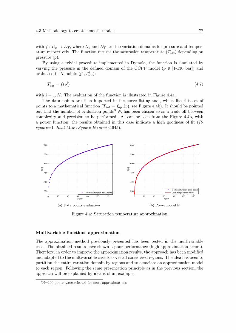
4.3 Methodology to create smooth models 77
with f : Dp → DT , where Dp and DT are the variation domains for pressure and temper-ature respectively. The function returns the saturation temperature (Tsat) depending onpressure (p).
By using a trivial procedure implemented in Dymola, the function is simulated byvarying the pressure in the defined domain of the CCPP model (p ∈ [1-130 bar]) andevaluated in N points (pi, T i
sat):
T isat = f(pi) (4.7)
with i = 1, N . The evaluation of the function is illustrated in Figure 4.4a.
The data points are then imported in the curve fitting tool, which fits this set ofpoints to a mathematical function (Tsat = fapp(p), see Figure 4.4b). It should be pointedout that the number of evaluation points3 N, has been chosen so as a trade-off betweencomplexity and precision to be performed. As can be seen from the Figure 4.4b, witha power function, the results obtained in this case indicate a high goodness of fit (R-square=1, Root Mean Square Error=0.1945).
0 20 40 60 80 100 120
350
400
450
500
550
600
p [bar]
T [K
]
Modelica function data points
(a) Data points evaluation
0 20 40 60 80 100 120
350
400
450
500
550
600
p [bar]
T [K
]
Modelica function data pointsData fitting: Power model
(b) Power model fit
Figure 4.4: Saturation temperature approximation
Multivariable functions approximation
The approximation method previously presented has been tested in the multivariablecase. The obtained results have shown a poor performance (high approximation errors).Therefore, in order to improve the approximation results, the approach has been modifiedand adapted to the multivariable case to cover all considered regions. The idea has been topartition the entire variation domain by regions and to associate an approximation modelto each region. Following the same presentation principle as in the previous section, theapproach will be explained by means of an example.
3N=100 points were selected for most approximations
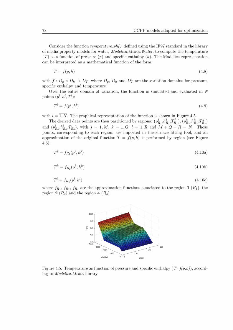
78 CCPP models adapted for optimization
Consider the function temperature ph(), defined using the IF97 standard in the libraryof media property models for water, Modelica.Media.Water, to compute the temperature(T ) as a function of pressure (p) and specific enthalpy (h). The Modelica representationcan be interpreted as a mathematical function of the form:
T = f(p, h) (4.8)
with f : Dp ×Dh → DT , where Dp, Dh and DT are the variation domains for pressure,specific enthalpy and temperature.
Over the entire domain of variation, the function is simulated and evaluated in Npoints (pi, hi, T i):
T i = f(pi, hi) (4.9)
with i = 1, N . The graphical representation of the function is shown in Figure 4.5.The derived data points are then partitioned by regions: (pjR1
,hjR1,T j
R1), (pkR2
,hkR2,T k
R2)
and (plR4,hlR4
,T lR4
), with j = 1,M , k = 1, Q, l = 1, R and M + Q + R = N . Thesepoints, corresponding to each region, are imported in the surface fitting tool, and anapproximation of the original function T = f(p, h) is performed by region (see Figure4.6):
T j = fR1(pj , hj) (4.10a)
T k = fR2(pk, hk) (4.10b)
T l = fR4(pl, hl) (4.10c)
where fR1, fR2
, fR4are the approximation functions associated to the region 1 (R1), the
region 2 (R2) and the region 4 (R4).
0
50
100
150
0
1000
2000
3000
4000200
400
600
800
1000
p [bar]h [kJ/kg]
T [K
]
Figure 4.5: Temperature as function of pressure and specific enthalpy (T=f(p,h)), accord-ing to Modelica.Media library

4.3 Methodology to create smooth models 79
0
50
100
150
2500
3000
3500
4000300
400
500
600
700
800
900
p [bar]h [kJ/kg]
T [K
]
R1
(a) Temperature evaluation region 1
0
50
100
150
0
500
1000
1500
2000200
300
400
500
600
p [bar]h [kJ/kg]
T [K
] R2
(b) Temperature evaluation region 2
0
50
100
150
0
1000
2000
3000350
400
450
500
550
600
650
p [bar]h [kJ/kg]
T [K
]
R4
(c) Temperature evaluation region 4
0
50
100
150
0
1000
2000
3000
4000200
400
600
800
1000
p [bar]h [kJ/kg]
T[K
]
f14
f42
R1
R4
R2
(d) Complete representation with boundaries
Figure 4.6: Temperature function decomposition by regions
Once the fitting problem for each region has been solved, the overall approximationis derived by connecting the functions associated to the regions in a continuous manner,in order to ensure its smoothness. In this case, the principle based on the Heaviside func-tion approximation, previously described, has been adapted by considering the boundaryfunctions among regions. Thus, rewriting equation (4.1) as:
∀x, y ∈ R, H(x, y) =
{0, x− fR(y) < 0
1, x− fR(y) ≥ 0(4.11)
the new smooth approximation used to define the continuous representation of the func-tion becomes:
∀x, y ∈ R, Hk(x, y) =1
1 + e−k(x−fR(y))(4.12)
where fR denotes the boundary function.
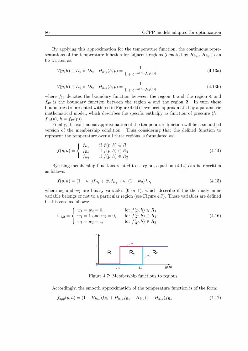
80 CCPP models adapted for optimization
By applying this approximation for the temperature function, the continuous repre-sentations of the temperature function for adjacent regions (denoted by Hk14 , Hk42) canbe written as:
∀(p, h) ∈ Dp ×Dh, Hk14(h, p) =1
1 + e−k(h−f14(p))(4.13a)
∀(p, h) ∈ Dp ×Dh, Hk42(h, p) =1
1 + e−k(h−f42(p))(4.13b)
where f14 denotes the boundary function between the region 1 and the region 4 andf42 is the boundary function between the region 4 and the region 2. In turn theseboundaries (represented with red in Figure 4.6d) have been approximated by a parametricmathematical model, which describes the specific enthalpy as function of pressure (h =f14(p), h = f42(p)).
Finally, the continuous approximation of the temperature function will be a smoothedversion of the membership condition. Thus considering that the defined function torepresent the temperature over all three regions is formulated as:
f(p, h) =
fR1, if f(p, h) ∈ R1
fR4, if f(p, h) ∈ R4
fR2, if f(p, h) ∈ R2
(4.14)
By using membership functions related to a region, equation (4.14) can be rewrittenas follows:
f(p, h) = (1− w1)fR1+ w2fR2
+ w1(1− w2)fR4(4.15)
where w1 and w2 are binary variables (0 or 1), which describe if the thermodynamicvariable belongs or not to a particular region (see Figure 4.7). These variables are definedin this case as follows:
w1,2 =
w1 = w2 = 0, for f(p, h) ∈ R1
w1 = 1 and w2 = 0, for f(p, h) ∈ R4
w1 = w2 = 1, for f(p, h) ∈ R2
(4.16)
f14 f42
0
1
R1 R4 R2
(p,h)
w
w
w
Figure 4.7: Membership functions to regions
Accordingly, the smooth approximation of the temperature function is of the form:
fapp(p, h) = (1−Hk14)fR1+Hk42fR2
+Hk14(1−Hk42)fR4(4.17)

4.3 Methodology to create smooth models 81
0
50
100
150
0
1000
2000
3000
4000200
400
600
800
1000
p [bar]h [kJ/kg]
T [K
]
(a) Temperature according to smooth approximation
0
50
100
150
0
1000
2000
3000
4000−40
−30
−20
−10
0
10
p [bar]h [kJ/kg]
e=T
−T
app [K
]
(b) Error representation (e = T − Tapp)
Figure 4.8: Smooth approximation of the temperature function and error evaluation
with Hk14 and Hk42 the smooth approximations described above. The graphical represen-tation of the function is illustrated in Figure 4.8a
Generally, by adopting this type of approach, the mathematical models obtained withthe fitting tools, are quite accurate, providing a good fit (R-square ≈ 1, RMSE close to 0).Also, the introduced errors by the smooth connection between the regions are quite small,resulting in a good approximation (see Figure 4.8b). The exception is the approximationin the first part of the variation interval ([1-5 bar]), where the errors are quite significant(around 35 K). These high errors derive from the approximation of the function for theregion 4, fR4
. A possible solution, in order to reduce these errors and to improve thealgorithm fit, is the refinement of the approximation function, by considering additionalpartitions of the regions into subregions. Such a method has been addressed in the caseof the functions that provide poor performance over entire domain of variation (e.g., thedensity as function of pressure and temperature has been partitioned in 5 sections). Forthe functions that have high errors only in the interval [1-5 bar], the obtained resultshave been considered as being in general satisfactory for the intended goals, and thereforean additional refining of the approximation was not necessary. Moreover, the variationdomain of the considered Modelica model in the case of a hot start-up sequence is higherthan this range. As it will be seen in the validation phase, the approach described inthis section enables to obtain a medium model quite consistent compared to the originalModelica one.
4.3.2 ThermoOpt library
In the modeling field, when a model or a library is designed, one of the first decision tobe taken is to specify the modeling purposes. As previously pointed out, the elementsof the ThermoPower library are primarily intended for simulation and are not designedwith the optimization purposes in mind. A new library, so-called ThermoOpt, has beendeveloped in this direction.

82 CCPP models adapted for optimization
4.3.2.1 Library purposes
In order to provide model components that can be used for model-based control appli-cations and in the same time that reflect as much as possible the behavior of the realsystem, the ThermoPower library’s components have been expanded and transformed.In other words, for each component of the ThermoPower library, corresponding to thereference model, a version in which the discontinuities have been reformulated by usingsmooth approximations has been developed. The idea has been to transform the existingmodels to be suitable for intended purposes and not re-create new models and librarycomponents. This enables, on one side, to keep the same structure of the model and onthe other side, the key aspect, to obtain a model suitable for optimization in terms ofissues such as complexity, accuracy and smoothness. Then these modified componentshave been included in ThermoOpt library, with a precise purpose, to be able to model,simulate, and optimize the control of a specific power plant. As in the ThermoPower ’scase, one of the principal objectives of the ThermoOpt library is to provide a base frame-work with common model parts, offering the possibility to the user to extend and adaptthe library’s elements for a particular application.
Thus, by providing a model library suitable for optimization, even if it does not havea general applicability, being limited to the CCPP start-up case at the time being, it canbe considered as an excellent way to package the modeling knowledge in a form that canbe further extended by other users with similar purposes.
In this context, the challenge was to find the best trade-off between the simplifica-tion/approximation of the model elements and their accuracy with respect to the originalrepresentations. What should the library cover and what should be excluded from thelibrary? These decisions affect the elaboration of model components since the designphase. In fact the library ThermoOpt aims to provide a basic framework for the modelingof the power plants elements, covering the engineering needs for an intuitive descriptionformat and the requirements of the efficient optimization algorithms.
4.3.2.2 Library principles
The ThermoOpt library closely follows the modeling principles adopted in ThermoPower.In the following sections, the main features of the model library ThermoOpt as well asthe differences compared to ThermoPower are outlined.
Library structure
The ThermoOpt library is structured into 9 packages: 7 main packages and 2 auxiliarypackages. Structuring of the packages in ThermoOpt is generally performed according totwo principles: an object decomposition and a subject decomposition, respectively. Theobject decomposition refers to the system subdivision into its physical parts, e.g., turbines,HRSG. In ThermoOpt, this partitioning is used in the package CCPP where the mainunits of the plant are included: GT, HRSG and ST. This subdivision facilitates the user’swork that can easily find unit models in the library. The subject decomposition deals withthe inheritance structure, that in our case is sparingly used to avoid the potential problemslinked to the inability of the optimization tools to address the inheritance mechanism. In
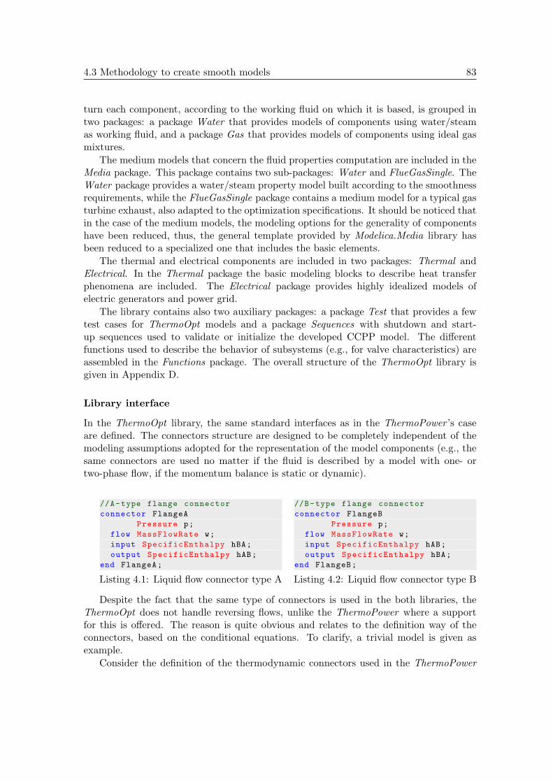
4.3 Methodology to create smooth models 83
turn each component, according to the working fluid on which it is based, is grouped intwo packages: a package Water that provides models of components using water/steamas working fluid, and a package Gas that provides models of components using ideal gasmixtures.
The medium models that concern the fluid properties computation are included in theMedia package. This package contains two sub-packages: Water and FlueGasSingle. TheWater package provides a water/steam property model built according to the smoothnessrequirements, while the FlueGasSingle package contains a medium model for a typical gasturbine exhaust, also adapted to the optimization specifications. It should be noticed thatin the case of the medium models, the modeling options for the generality of componentshave been reduced, thus, the general template provided by Modelica.Media library hasbeen reduced to a specialized one that includes the basic elements.
The thermal and electrical components are included in two packages: Thermal andElectrical. In the Thermal package the basic modeling blocks to describe heat transferphenomena are included. The Electrical package provides highly idealized models ofelectric generators and power grid.
The library contains also two auxiliary packages: a package Test that provides a fewtest cases for ThermoOpt models and a package Sequences with shutdown and start-up sequences used to validate or initialize the developed CCPP model. The differentfunctions used to describe the behavior of subsystems (e.g., for valve characteristics) areassembled in the Functions package. The overall structure of the ThermoOpt library isgiven in Appendix D.
Library interface
In the ThermoOpt library, the same standard interfaces as in the ThermoPower ’s caseare defined. The connectors structure are designed to be completely independent of themodeling assumptions adopted for the representation of the model components (e.g., thesame connectors are used no matter if the fluid is described by a model with one- ortwo-phase flow, if the momentum balance is static or dynamic).
//A-type flange connector
connector FlangeA
Pressure p;
flow MassFlowRate w;
input SpecificEnthalpy hBA;
output SpecificEnthalpy hAB;
end FlangeA;
Listing 4.1: Liquid flow connector type A
//B-type flange connector
connector FlangeB
Pressure p;
flow MassFlowRate w;
input SpecificEnthalpy hAB;
output SpecificEnthalpy hBA;
end FlangeB;
Listing 4.2: Liquid flow connector type B
Despite the fact that the same type of connectors is used in the both libraries, theThermoOpt does not handle reversing flows, unlike the ThermoPower where a supportfor this is offered. The reason is quite obvious and relates to the definition way of theconnectors, based on the conditional equations. To clarify, a trivial model is given asexample.
Consider the definition of the thermodynamic connectors used in the ThermoPower

84 CCPP models adapted for optimization
library to describe the flanges of the components that carry a water/steam flow, presentedin Listings 4.1 and 4.2.
In Listings 4.1 and 4.2, p is the fluid pressure, representing the potential variable, w isthe mass flow rate entering the component, representing the flow variable, hAB and hBA
are the specific enthalpies of the fluid corresponding to the flow direction from a flangeof A-type to a flange of B-type and vice versa respectively. Although the two types ofconnector are formally equivalent, the basic rule when two components are connected isthat the connection has always to be made between two flanges of complementary type.These types of connectors enable to deal with reversing flows in a quite simple way. Thischaracteristic is illustrated in Listing 4.3 by means of a simple model describing a vesselwith a constant quantity of liquid.
The reversing flow support in the models is specified by considering two conditionalexpressions, thus, the example equations give hi = Inl.hBA and ho = h, when the massflow is positive, and hi = h and ho = Out.hAB, when the mass flow is negative. Theseexpressions can introduce discontinuities, making the optimization problem to be non-smooth. Consequently, in ThermoOpt the conditional expressions have been eliminatedfrom the library models, resulting in model components without reversing flow support(see Listing 4.4).
model SimpleV "ThermoPower version"
FlangeA Inl;
FlangeB Out;
parameter Mass Ml=10 "Fluid mass";
Pressure p;
SpecificEnthalpy h "of Fluid";
SpecificEnthalpy hi "at Inlet";
SpecificEnthalpy ho "at Outlet";
equation
//Mass balance
0 = Inl.w + Out.w;
// Energy balance
Ml*der(h) = Inl.w*hi + Out.w*ho;
// Boundary conditions
hi = if Inl.w >= 0 then Inl.hBA
else h;
ho = if Out.w >= 0 then Out.hAB
else h;
Inl.hAB = h;
Out.hBA = h;
Inl.p = p;
Out.p = p;
end SimpleV;
Listing 4.3: Reversing flow example
model SimpleV "ThermoOpt version"
FlangeA Inl;
FlangeB Out;
parameter Mass Ml=10 "Fluid mass";
Pressure p;
SpecificEnthalpy h "of Fluid";
SpecificEnthalpy hi "at Inlet";
SpecificEnthalpy ho "at Outlet";
equation
//Mass balance
0 = Inl.w + Out.w;
// Energy balance
Ml*der(h) = Inl.w*hi + Out.w*ho;
// Boundary conditions
hi = Inl.hBA;
ho = h;
Inl.hAB = h;
Out.hBA = h;
Inl.p = p;
Out.p = p;
end SimpleV;
Listing 4.4: Non-reversing flow example
In general, when models are supposed to not support reversing flows, additional in-formation in connectors (such as specification of the inlet/outlet specific enthalpies) arenot required. Although, to keep the compatibility between the library’s elements, thestructure of the connectors in ThermoOpt remains the same as in the ThemoPower li-
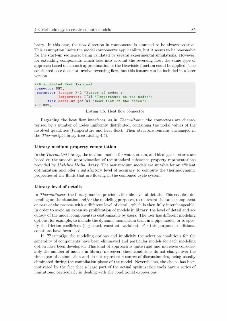
4.3 Methodology to create smooth models 85
brary. In this case, the flow direction in components is assumed to be always positive.This assumption limits the model components applicability, but it seems to be reasonablefor the start-up sequence, being validated by several experimental simulations. However,for extending components which take into account the reversing flow, the same type ofapproach based on smooth approximation of the Heaviside function could be applied. Theconsidered case does not involve reversing flow, but this feature can be included in a laterversion.
// Distributed Heat Terminal
connector DHT;
parameter Integer N=2 "Number of nodes";
Temp erature T[N] "Temperature at the nodes";
flow Heat Flux phi[N] "Heat flux at the nodes";
end DHT;
Listing 4.5: Heat flow connector
Regarding the heat flow interfaces, as in ThemoPower, the connectors are charac-terized by a number of nodes uniformly distributed, containing the nodal values of theinvolved quantities (temperature and heat flux). Their structure remains unchanged inthe ThermoOpt library (see Listing 4.5).
Library medium property computation
In the ThermoOpt library, the medium models for water, steam, and ideal gas mixtures arebased on the smooth approximation of the standard substance property representationsprovided by Modelica.Media library. The new medium models are suitable for an efficientoptimization and offer a satisfactory level of accuracy to compute the thermodynamicproperties of the fluids that are flowing in the combined cycle system.
Library level of details
In ThermoPower, the library models provide a flexible level of details. This enables, de-pending on the situation and/or the modeling purposes, to represent the same componentor part of the process with a different level of detail, which is then fully interchangeable.In order to avoid an excessive proliferation of models in library, the level of detail and ac-curacy of the model components is customizable by users. The user has different modelingoptions, for example, to include the dynamic momentum term in a pipe model, or to spec-ify the friction coefficient (neglected, constant, variable). For this purpose, conditionalequations have been used.
In ThermoOpt the modeling options and implicitly the selection conditions for thegenerality of components have been eliminated and particular models for each modelingoption have been developed. This kind of approach is quite rigid and increases consider-ably the number of models in library, moreover, these conditions do not change over thetime span of a simulation and do not represent a source of discontinuities, being usuallyeliminated during the compilation phase of the model. Nevertheless, the choice has beenmotivated by the fact that a large part of the actual optimization tools have a series oflimitations, particularly in dealing with the conditional expressions.

86 CCPP models adapted for optimization
The modeling assumptions adopted in the optimization library match those fromthe simulation one, the difference is related to the representation of the models. Thus,in ThermoOpt the components of interest from the ThermoPower library, in particularthose components corresponding to the developed CCPP model, have been implementedin a form that is suitable for optimization, by means of smooth approximation procedurepresented above in this chapter. It should be noticed that unlike the ThermoPower thatprovides a wide range of model components for power plants modeling, the ThermoOpt ’smodels range is narrower, including only the elementary components necessary to describea combined cycle model. A few examples of model components implemented as Modelicacode are reported in Appendix E. The library elements have been validated against thedata obtained by the ThermoPower models. The validation procedure will be presentedin the sequel.
4.3.3 Library models validation
The validation of the optimization library elements has been performed by comparingtheir responses, to the variation of the input signals, with the ones obtained by the Ther-moPower ’s models. The validation procedure presented in this section strictly refers todemonstrate the consistency of ThermoOpt ’s components with respect to the developedCCPP simulator. Thus, the procedure consists in a systematic replacement of the originalelements of the CCPP simulator based on ThermoPower with the ones provided by Ther-moOpt library; then the simulation scenarios are separately applied on the new CCPP”test-model” as well as on the reference simulator, and the so obtained evolution of themain parameters are graphically compared.
The reliability of the library’s components has been investigated through simulationby means of several typical scenarios for the start-up procedure. The main two validationtests and the results of these tests are presented in the following.
Scenario I
The first scenario refers to a ramp variation of the GT load and of the bypass position.The GT load is gradually increased until 30% of maximal threshold, following a ramp withthe slope of 2.25%/min, applied at 120 seconds. According to a ramp variation profilewith a slope of 40%/min, the bypass valve is opened up to about 36 %, at 600 seconds.The variations applied on the GT load and on the bypass position are presented in Figures4.9a and 4.9b. The other signal inputs have been maintained constant and their valuesas well as the model initialization correspond to the hot start-up phase specified in theprevious chapter (see Section 3.4.5).
Scenario II
The second scenario deals with a gradual variation of the GT load, which is increased from7.5% (the initial state of GT, corresponding to a power of 17.6 MW) until 90% of nominalload, following a ramp profile with a slope of approx. 4%/min, applied after 180 seconds.Also, a ramp variation profile with a slope of 60%/min is applied on the ST throttle valveafter 600 seconds. The variations applied on the GT load and on the ST valve position

4.3 Methodology to create smooth models 87
are illustrated in Figures 4.9c and 4.9d. During the scenario, the ST is assumed to beconnected to the grid and the other inputs are kept constant, corresponding to the hotstart-up state.
0 500 1000 1500 2000 2500 3000 3500 40000.05
0.1
0.15
0.2
0.25
0.3
0.35
0.4
Time [s]
GT
Loa
d [n
orm
aliz
ed]
GT Load variation
(a) Scenario I: GT Load ramp variation
0 500 1000 1500 2000 2500 3000 3500 4000
0.2
0.25
0.3
0.35
0.4
Time [s]B
ypas
s op
enin
g [p
.u.]
Bypass variation
(b) Scenario I: Bypass ramp variation
0 500 1000 1500 2000 2500 3000 3500 40000
0.1
0.2
0.3
0.4
0.5
0.6
0.7
0.8
0.9
1
Time [s]
GT
Loa
d [n
orm
aliz
ed]
GT Load variation
(c) Scenario II: GT Load ramp variation
0 500 1000 1500 2000 2500 3000 3500 40000
0.1
0.2
0.3
0.4
0.5
0.6
0.7
Time [s]
ST
thro
ttle
valv
e op
enin
g [p
.u.]
ST throttle valve variation
(d) Scenario II: ST throttle ramp variation
Figure 4.9: Scenarios I and II: Applied variations of the input variables
4.3.3.1 Medium models validation
To validate the simplified/approximated models for the fluid properties calculation im-plemented in the ThermoOpt library, a new version of the CCPP reference model hasbeen derived. This new model has been obtained by replacing the standard Mediummodels with approximated ones, keeping the original components. Then, the validationscenarios presented above have been applied on both models (CCPP reference model andCCPP model based on the ThermoOpt Medium models), and their responses have beencompared.
In general the parameters that have been investigated are the temperature, pressureand the mass flow rate of the steam. Following the applied scenarios, the steam flow rate
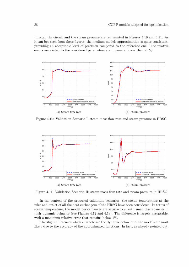
88 CCPP models adapted for optimization
through the circuit and the steam pressure are represented in Figures 4.10 and 4.11. Asit can bee seen from these figures, the medium models approximation is quite consistent,providing an acceptable level of precision compared to the reference one. The relativeerrors associated to the considered parameters are in general lower than 2.5%.
0 500 1000 1500 2000 2500 3000 3500 40005
10
15
20
25
30
35
Time [s]
w [k
g/s]
reference modelmodel with ThermoOpt Medium
(a) Steam flow rate
0 500 1000 1500 2000 2500 3000 3500 400065
70
75
80
85
90
95
100
105
110
115
Time [s]p
[bar
]
reference modelmodel with ThermoOpt Medium
(b) Steam pressure
Figure 4.10: Validation Scenario I: steam mass flow rate and steam pressure in HRSG
0 500 1000 1500 2000 2500 3000 3500 40000
10
20
30
40
50
60
70
80
Time [s]
w [k
g/s]
reference modelmodel with ThermoOpt Medium
(a) Steam flow rate
0 500 1000 1500 2000 2500 3000 3500 400060
70
80
90
100
110
120
Time [s]
p [b
ar]
reference modelmodel with ThermoOpt Medium
(b) Steam pressure
Figure 4.11: Validation Scenario II: steam mass flow rate and steam pressure in HRSG
In the context of the proposed validation scenarios, the steam temperature at theinlet and outlet of all the heat exchangers of the HRSG have been considered. In terms ofsteam temperature, the model performances are satisfactory, with small discrepancies intheir dynamic behavior (see Figures 4.12 and 4.13). The difference is largely acceptable,with a maximum relative error that remains below 1%.
The slight differences which characterize the dynamic behavior of the models are mostlikely due to the accuracy of the approximated functions. In fact, as already pointed out,

4.3 Methodology to create smooth models 89
0 500 1000 1500 2000 2500 3000 3500 4000294.4
294.6
294.8
295
295.2
295.4
295.6
Time [s]
T [K
]
reference modelmodel with ThermoOpt Medium
(a) ECO inlet steam temperature
0 500 1000 1500 2000 2500 3000 3500 4000545
550
555
560
565
570
575
580
585
590
Time [s]
T [K
]
reference modelmodel with ThermoOpt Medium
(b) ECO outlet steam temperature
0 500 1000 1500 2000 2500 3000 3500 4000550
555
560
565
570
575
580
585
590
595
Time [s]
T [K
]
reference modelmodel with ThermoOpt Medium
(c) EV inlet steam temperature
0 500 1000 1500 2000 2500 3000 3500 4000550
555
560
565
570
575
580
585
590
595
Time [s]
T [K
]
reference modelmodel with ThermoOpt Medium
(d) EV outlet steam temperature
0 500 1000 1500 2000 2500 3000 3500 4000550
555
560
565
570
575
580
585
590
595
Time [s]
T [K
]
reference modelmodel with ThermoOpt Medium
(e) SH inlet steam temperature
0 500 1000 1500 2000 2500 3000 3500 4000560
580
600
620
640
660
680
700
Time [s]
T [K
]
reference modelmodel with ThermoOpt Medium
(f) SH outlet steam temperature
Figure 4.12: Validation Scenario I: steam temperature in HRSG
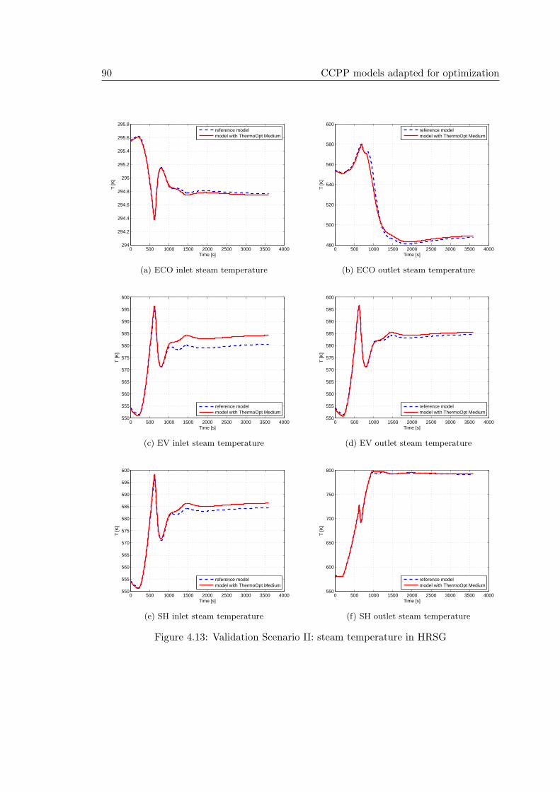
90 CCPP models adapted for optimization
0 500 1000 1500 2000 2500 3000 3500 4000294
294.2
294.4
294.6
294.8
295
295.2
295.4
295.6
295.8
Time [s]
T [K
]
reference modelmodel with ThermoOpt Medium
(a) ECO inlet steam temperature
0 500 1000 1500 2000 2500 3000 3500 4000480
500
520
540
560
580
600
Time [s]
T [K
]
reference modelmodel with ThermoOpt Medium
(b) ECO outlet steam temperature
0 500 1000 1500 2000 2500 3000 3500 4000550
555
560
565
570
575
580
585
590
595
600
Time [s]
T [K
]
reference modelmodel with ThermoOpt Medium
(c) EV inlet steam temperature
0 500 1000 1500 2000 2500 3000 3500 4000550
555
560
565
570
575
580
585
590
595
600
Time [s]
T [K
]
reference modelmodel with ThermoOpt Medium
(d) EV outlet steam temperature
0 500 1000 1500 2000 2500 3000 3500 4000550
555
560
565
570
575
580
585
590
595
600
Time [s]
T [K
]
reference modelmodel with ThermoOpt Medium
(e) SH inlet steam temperature
0 500 1000 1500 2000 2500 3000 3500 4000550
600
650
700
750
800
Time [s]
T [K
]
reference modelmodel with ThermoOpt Medium
(f) SH outlet steam temperature
Figure 4.13: Validation Scenario II: steam temperature in HRSG
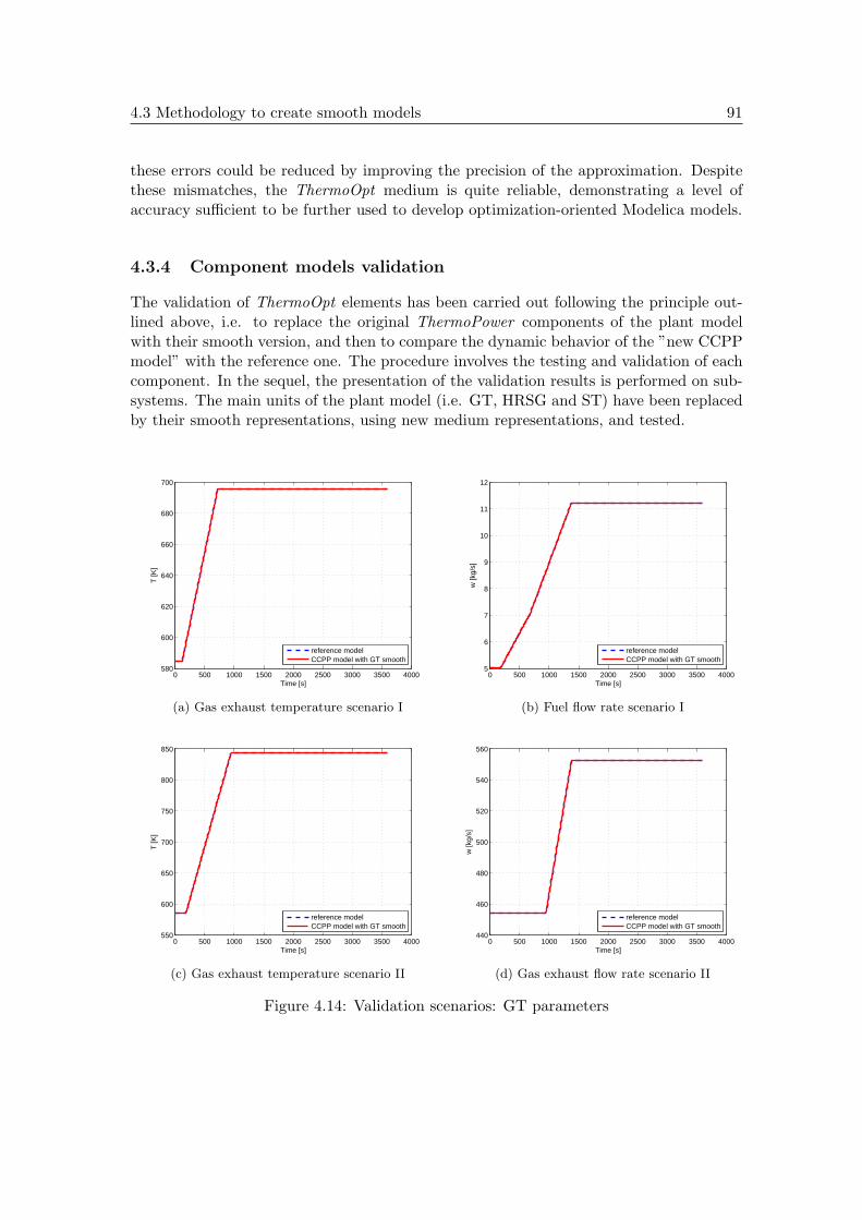
4.3 Methodology to create smooth models 91
these errors could be reduced by improving the precision of the approximation. Despitethese mismatches, the ThermoOpt medium is quite reliable, demonstrating a level ofaccuracy sufficient to be further used to develop optimization-oriented Modelica models.
4.3.4 Component models validation
The validation of ThermoOpt elements has been carried out following the principle out-lined above, i.e. to replace the original ThermoPower components of the plant modelwith their smooth version, and then to compare the dynamic behavior of the ”new CCPPmodel” with the reference one. The procedure involves the testing and validation of eachcomponent. In the sequel, the presentation of the validation results is performed on sub-systems. The main units of the plant model (i.e. GT, HRSG and ST) have been replacedby their smooth representations, using new medium representations, and tested.
0 500 1000 1500 2000 2500 3000 3500 4000580
600
620
640
660
680
700
Time [s]
T [K
]
reference modelCCPP model with GT smooth
(a) Gas exhaust temperature scenario I
0 500 1000 1500 2000 2500 3000 3500 40005
6
7
8
9
10
11
12
Time [s]
w [k
g/s]
reference modelCCPP model with GT smooth
(b) Fuel flow rate scenario I
0 500 1000 1500 2000 2500 3000 3500 4000550
600
650
700
750
800
850
Time [s]
T [K
]
reference modelCCPP model with GT smooth
(c) Gas exhaust temperature scenario II
0 500 1000 1500 2000 2500 3000 3500 4000440
460
480
500
520
540
560
Time [s]
w [k
g/s]
reference modelCCPP model with GT smooth
(d) Gas exhaust flow rate scenario II
Figure 4.14: Validation scenarios: GT parameters
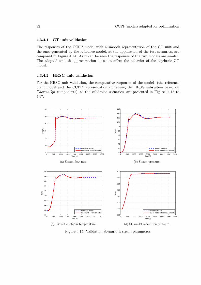
92 CCPP models adapted for optimization
4.3.4.1 GT unit validation
The responses of the CCPP model with a smooth representation of the GT unit andthe ones generated by the reference model, at the application of the test scenarios, arecompared in Figure 4.14. As it can be seen the responses of the two models are similar.The adopted smooth approximation does not affect the behavior of the algebraic GTmodel.
4.3.4.2 HRSG unit validation
For the HRSG unit validation, the comparative responses of the models (the referenceplant model and the CCPP representation containing the HRSG subsystem based onThermoOpt components), to the validation scenarios, are presented in Figures 4.15 to4.17.
0 500 1000 1500 2000 2500 3000 3500 40005
10
15
20
25
30
35
Time [s]
w [k
g/s]
reference modelmodel with HRSG smooth
(a) Steam flow rate
0 500 1000 1500 2000 2500 3000 3500 400065
70
75
80
85
90
95
100
105
110
115
Time [s]
p [b
ar]
reference modelmodel with HRSG smooth
(b) Steam pressure
0 500 1000 1500 2000 2500 3000 3500 4000550
555
560
565
570
575
580
585
590
595
Time [s]
T [K
]
reference modelmodel with HRSG smooth
(c) EV outlet steam temperature
0 500 1000 1500 2000 2500 3000 3500 4000560
580
600
620
640
660
680
700
Time [s]
T [K
]
reference modelCCPP model with HRSG smooth
(d) SH outlet steam temperature
Figure 4.15: Validation Scenario I: steam parameters
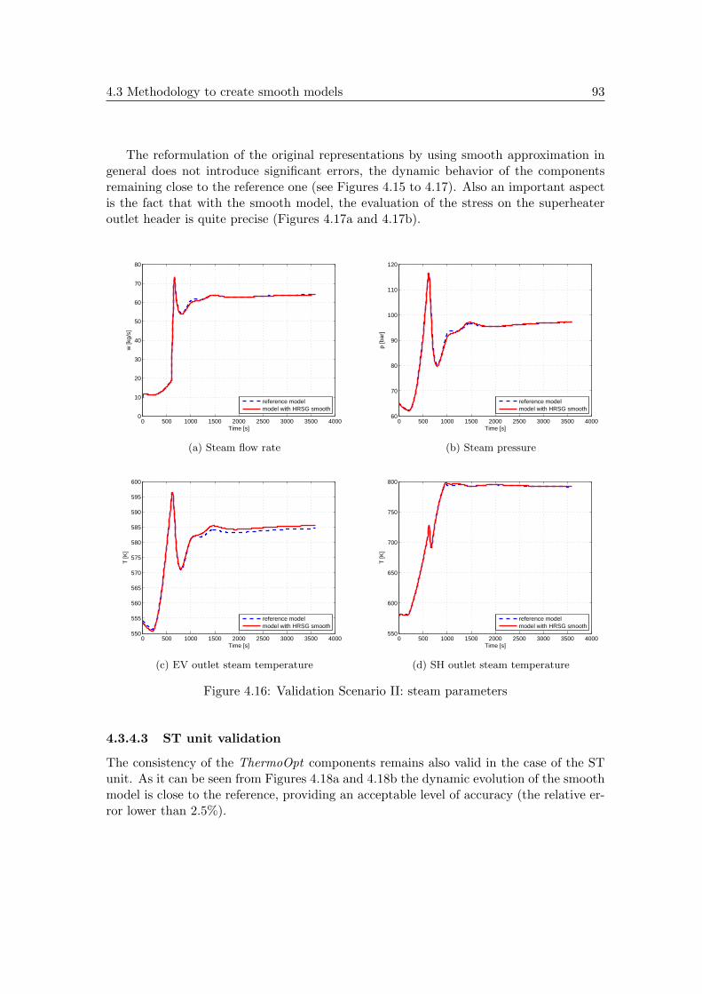
4.3 Methodology to create smooth models 93
The reformulation of the original representations by using smooth approximation ingeneral does not introduce significant errors, the dynamic behavior of the componentsremaining close to the reference one (see Figures 4.15 to 4.17). Also an important aspectis the fact that with the smooth model, the evaluation of the stress on the superheateroutlet header is quite precise (Figures 4.17a and 4.17b).
0 500 1000 1500 2000 2500 3000 3500 40000
10
20
30
40
50
60
70
80
Time [s]
w [k
g/s]
reference modelmodel with HRSG smooth
(a) Steam flow rate
0 500 1000 1500 2000 2500 3000 3500 400060
70
80
90
100
110
120
Time [s]
p [b
ar]
reference modelmodel with HRSG smooth
(b) Steam pressure
0 500 1000 1500 2000 2500 3000 3500 4000550
555
560
565
570
575
580
585
590
595
600
Time [s]
T [K
]
reference modelmodel with HRSG smooth
(c) EV outlet steam temperature
0 500 1000 1500 2000 2500 3000 3500 4000550
600
650
700
750
800
Time [s]
T [K
]
reference modelmodel with HRSG smooth
(d) SH outlet steam temperature
Figure 4.16: Validation Scenario II: steam parameters
4.3.4.3 ST unit validation
The consistency of the ThermoOpt components remains also valid in the case of the STunit. As it can be seen from Figures 4.18a and 4.18b the dynamic evolution of the smoothmodel is close to the reference, providing an acceptable level of accuracy (the relative er-ror lower than 2.5%).
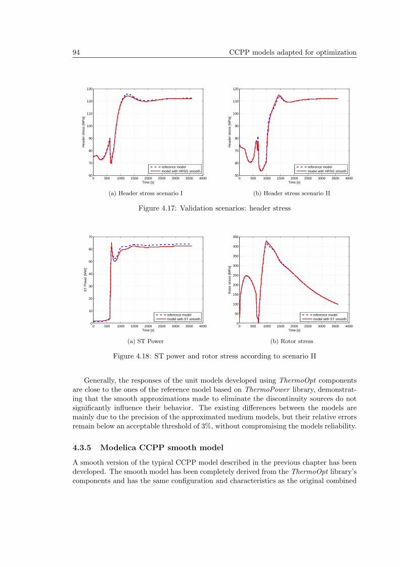
94 CCPP models adapted for optimization
0 500 1000 1500 2000 2500 3000 3500 400060
70
80
90
100
110
120
130
Time [s]
Hea
der
stre
ss [M
Pa]
reference modelmodel with HRSG smooth
(a) Header stress scenario I
0 500 1000 1500 2000 2500 3000 3500 400050
60
70
80
90
100
110
120
Time [s]
Hea
der
stre
ss [M
Pa]
reference modelmodel with HRSG smooth
(b) Header stress scenario II
Figure 4.17: Validation scenarios: header stress
0 500 1000 1500 2000 2500 3000 3500 40000
10
20
30
40
50
60
70
Time [s]
ST
Pow
er [M
W]
reference modelmodel with ST smooth
(a) ST Power
0 500 1000 1500 2000 2500 3000 3500 40000
50
100
150
200
250
300
350
400
450
Time [s]
Rot
or s
tres
s [M
Pa]
reference modelmodel with ST smooth
(b) Rotor stress
Figure 4.18: ST power and rotor stress according to scenario II
Generally, the responses of the unit models developed using ThermoOpt componentsare close to the ones of the reference model based on ThermoPower library, demonstrat-ing that the smooth approximations made to eliminate the discontinuity sources do notsignificantly influence their behavior. The existing differences between the models aremainly due to the precision of the approximated medium models, but their relative errorsremain below an acceptable threshold of 3%, without compromising the models reliability.
4.3.5 Modelica CCPP smooth model
A smooth version of the typical CCPP model described in the previous chapter has beendeveloped. The smooth model has been completely derived from the ThermoOpt library’scomponents and has the same configuration and characteristics as the original combined
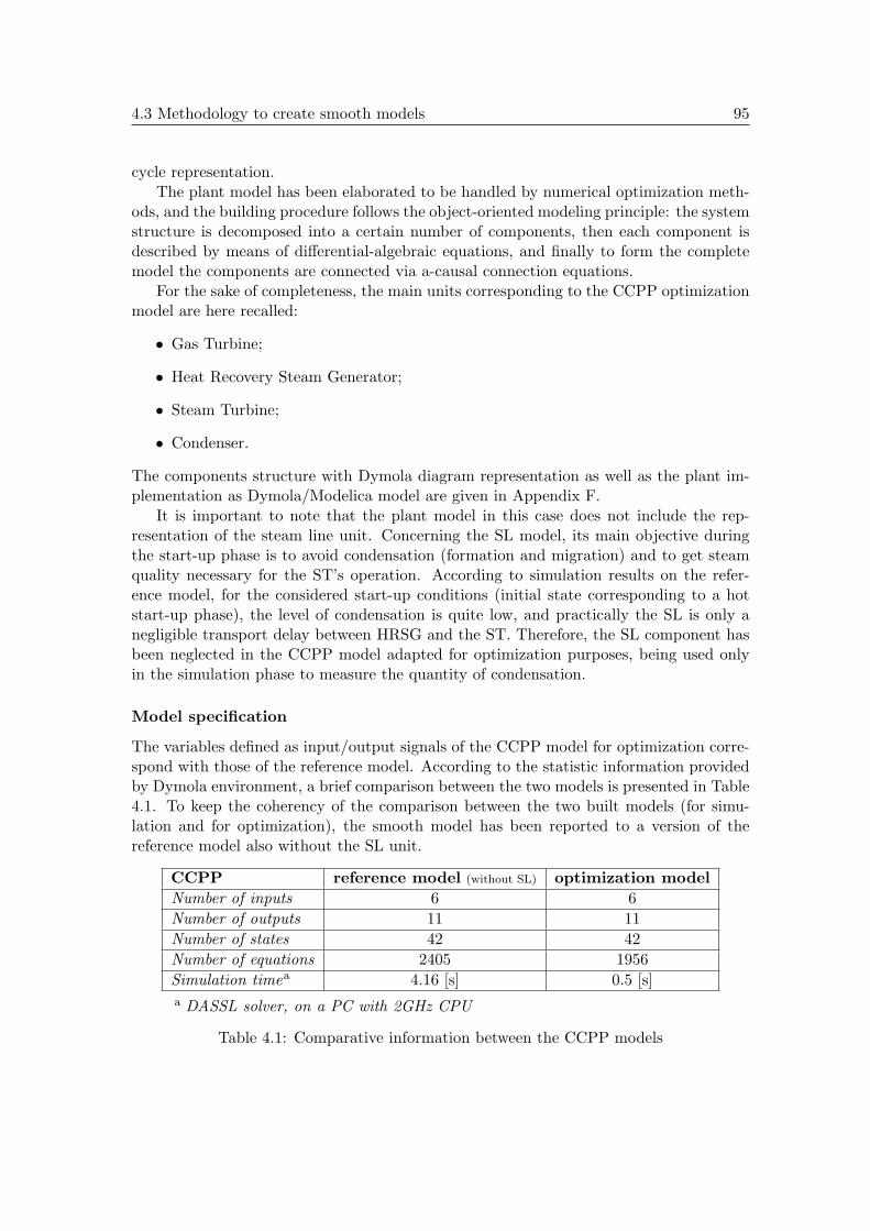
4.3 Methodology to create smooth models 95
cycle representation.The plant model has been elaborated to be handled by numerical optimization meth-
ods, and the building procedure follows the object-oriented modeling principle: the systemstructure is decomposed into a certain number of components, then each component isdescribed by means of differential-algebraic equations, and finally to form the completemodel the components are connected via a-causal connection equations.
For the sake of completeness, the main units corresponding to the CCPP optimizationmodel are here recalled:
• Gas Turbine;
• Heat Recovery Steam Generator;
• Steam Turbine;
• Condenser.
The components structure with Dymola diagram representation as well as the plant im-plementation as Dymola/Modelica model are given in Appendix F.
It is important to note that the plant model in this case does not include the rep-resentation of the steam line unit. Concerning the SL model, its main objective duringthe start-up phase is to avoid condensation (formation and migration) and to get steamquality necessary for the ST’s operation. According to simulation results on the refer-ence model, for the considered start-up conditions (initial state corresponding to a hotstart-up phase), the level of condensation is quite low, and practically the SL is only anegligible transport delay between HRSG and the ST. Therefore, the SL component hasbeen neglected in the CCPP model adapted for optimization purposes, being used onlyin the simulation phase to measure the quantity of condensation.
Model specification
The variables defined as input/output signals of the CCPP model for optimization corre-spond with those of the reference model. According to the statistic information providedby Dymola environment, a brief comparison between the two models is presented in Table4.1. To keep the coherency of the comparison between the two built models (for simu-lation and for optimization), the smooth model has been reported to a version of thereference model also without the SL unit.
CCPP reference model (without SL) optimization model
Number of inputs 6 6
Number of outputs 11 11
Number of states 42 42
Number of equations 2405 1956
Simulation timea 4.16 [s] 0.5 [s]
a DASSL solver, on a PC with 2GHz CPU
Table 4.1: Comparative information between the CCPP models

96 CCPP models adapted for optimization
The both models can be rapidly simulated, but nevertheless a significant improvementin the simulation time of the smooth model compared to the reference one (a time reduc-tion of about 90%) can be observed. Therefore, only considering this aspect (simulationtime), the effect of the applied transformations is quite important.
4.3.6 Model validation
As in the validation study of the ThermoOpt library, the reliability and consistency ofthe CCPP smooth model have been investigated by means of several scenarios judgedas representative for the start-up phase by engineers. These test scenarios have beenderived from a standard start-up procedure and can reflect real transient operating con-ditions of the plant. Also specific scenarios corresponding to the start-up stages have beenconsidered in order to make a phase by phase validation.
The validation of the smooth CCPP model has been made by strictly comparing itsresponses to the variation of the input signals, with the ones obtained by the previouslydescribed CCPP simulator, considering the same initial conditions for both models. In thissection, additionally to the validation scenarios previously presented, two other scenarioshave been studied in order to get more confidence in the smooth model consistency: asimple scenario which involves the variation of the input signals, and an experimental testthat replicates a classical start-up procedure.
Scenario III
This scenario corresponds to a step variation of the desuperheater flow rate and to aGT load profile that follows a ramp with a slope of approximately 0.65%/min, appliedafter 180 seconds (see Figures 4.19a). The step variation on the desuperheater flow rate
0 500 1000 1500 2000 2500 3000 3500 40000.1
0.15
0.2
0.25
0.3
0.35
0.4
Time [s]
GT
Loa
d [n
orm
aliz
ed]
GT Load variation
(a) GT Load ramp variation
0 500 1000 1500 2000 2500 3000 3500 40000
0.02
0.04
0.06
0.08
0.1
0.12
0.14
0.16
0.18
0.2
Time [s]
DS
H [p
.u.]
DSH step variation
(b) Desuperheater step variation
Figure 4.19: Scenario III: Applied variations of the input variables
has an amplitude of 10% and is applied at 1500 seconds (see Figures 4.19b). The initialconditions assumed in this case are:
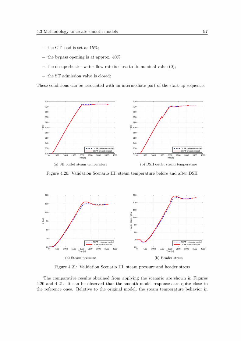
4.3 Methodology to create smooth models 97
− the GT load is set at 15%;
− the bypass opening is at approx. 40%;
− the desuperheater water flow rate is close to its nominal value (0);
− the ST admission valve is closed;
These conditions can be associated with an intermediate part of the start-up sequence.
0 500 1000 1500 2000 2500 3000 3500 4000620
630
640
650
660
670
680
690
700
710
720
Time [s]
T [K
]
CCPP reference modelCCPP smooth model
(a) SH outlet steam temperature
0 500 1000 1500 2000 2500 3000 3500 4000620
630
640
650
660
670
680
690
700
710
720
Time [s]
T [K
]
CCPP reference modelCCPP smooth model
(b) DSH outlet steam temperature
Figure 4.20: Validation Scenario III: steam temperature before and after DSH
0 500 1000 1500 2000 2500 3000 3500 400060
70
80
90
100
110
120
Time [s]
p [b
ar]
CCPP reference modelCCPP smooth model
(a) Steam pressure
0 500 1000 1500 2000 2500 3000 3500 400060
70
80
90
100
110
120
130
Time [s]
Hea
der
stre
ss [M
Pa]
CCPP reference modelCCPP smooth model
(b) Header stress
Figure 4.21: Validation Scenario III: steam pressure and header stress
The comparative results obtained from applying the scenario are shown in Figures4.20 and 4.21. It can be observed that the smooth model responses are quite close tothe reference ones. Relative to the original model, the steam temperature behavior in

98 CCPP models adapted for optimization
the smooth model is characterized by a slight difference (see Figure 4.20). In termsof steam pressure, the discrepancy between the two models is considered as acceptable,the relative error being below 2.5% (see Figure 4.21a). In general, the result of thesedifferences, mainly between pressures, can also be seen in the evaluation of stress on thesuperheater outlet header (Figure 4.21a).
Scenario IV
This scenario replicates a simplified start-up sequence. Considering the initial conditioncorresponding to the hot start-up phase, with GT synchronized and connected to thegrid, the scenario follows the steps of the start-up sequence described in Section 2.2.5.6,namely:
1. Temperature matching : the HRSG metal is gradually warmed (during 1500 seconds)in order to limit the thermal stress. Using the bypass, the pressure in circuit ismaintained close to the value required by the ST (60 bar);
2. ST Start-up: the ST admission starts after 2000 seconds when the steam conditionsare fulfilled (i.e. steam temperature higher than ST metal temperature, steampressure above 60 bar). At 2100 seconds, the ST is synchronized to the grid.
3. Increasing load : the bypass is closed (2300 seconds) and the ST valve is graduallyopened (completely open at 3900 seconds). The GT and ST loads are increaseduntil they reach their nominal values.
As in previous cases, the difference between the models is below the relative tolerance of2.5% with respect to the main plant variables (see Figures 4.22 to 4.24).
0 1000 2000 3000 4000 5000 6000550
600
650
700
750
800
850
Time [s]
T [K
]
CCPP reference modelCCPP smooth model
(a) Steam temperature
0 1000 2000 3000 4000 5000 600050
60
70
80
90
100
110
120
130
Time [s]
p [b
ar]
CCPP reference modelCCPP smooth model
(b) Steam pressure
Figure 4.22: Validation Scenario IV: temperature and pressure of the steam
The results of the validation tests show the smooth model consistency and denote that itis accurate enough to be further used for control purposes. Although there are some small
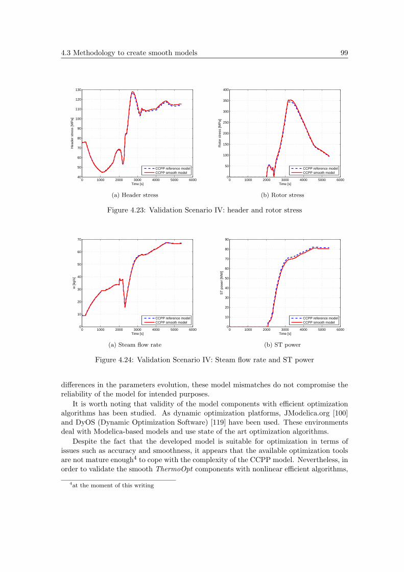
4.3 Methodology to create smooth models 99
0 1000 2000 3000 4000 5000 600040
50
60
70
80
90
100
110
120
130
Time [s]
Hea
der
stre
ss [M
Pa]
CCPP reference modelCCPP smooth model
(a) Header stress
0 1000 2000 3000 4000 5000 60000
50
100
150
200
250
300
350
400
Time [s]
Rot
or s
tres
s [M
Pa]
CCPP reference modelCCPP smooth model
(b) Rotor stress
Figure 4.23: Validation Scenario IV: header and rotor stress
0 1000 2000 3000 4000 5000 60000
10
20
30
40
50
60
70
Time [s]
w [k
g/s]
CCPP reference modelCCPP smooth model
(a) Steam flow rate
0 1000 2000 3000 4000 5000 60000
10
20
30
40
50
60
70
80
90
Time [s]
ST
pow
er [M
W]
CCPP reference modelCCPP smooth model
(b) ST power
Figure 4.24: Validation Scenario IV: Steam flow rate and ST power
differences in the parameters evolution, these model mismatches do not compromise thereliability of the model for intended purposes.
It is worth noting that validity of the model components with efficient optimizationalgorithms has been studied. As dynamic optimization platforms, JModelica.org [100]and DyOS (Dynamic Optimization Software) [119] have been used. These environmentsdeal with Modelica-based models and use state of the art optimization algorithms.
Despite the fact that the developed model is suitable for optimization in terms ofissues such as accuracy and smoothness, it appears that the available optimization toolsare not mature enough4 to cope with the complexity of the CCPP model. Nevertheless, inorder to validate the smooth ThermoOpt components with nonlinear efficient algorithms,
4at the moment of this writing

100 CCPP models adapted for optimization
the optimization problems based on the subsystems of the CCPP model have been solvedwith JModelica.org tool. The optimization problem formulation as well as the obtainedresults will be presented in the next chapter.
4.4 Conclusions
The approach adopted in this chapter had as objective the development of Modelicamodels which can be handled by efficient nonlinear optimization algorithms. In generalsuch algorithms impose a series of restrictions on the model structure which limit theirapplicability. Therefore certain transformations in order to obtain Modelica models readyto be used for an effective optimization are required.
In this direction, a methodology that aims at transforming a physical simulation modelsuitable for description of a CCPP start-up behavior, to one adapted for model-basedcontrol applications has been proposed. The method enables to keep the same modelstructure as the reference one and to create models suitable for optimization with respectto complexity, accuracy and smoothness. The reformulation of the models structure isbased on continuous approximations.
The modified components have been included in a new library, ThermoOpt. Even if thelibrary has a limited operating range, its model components are suitable for optimizationpurposes, covering engineering needs for an intuitive description format of the powerplants and efficient optimization algorithms requirements.
By using the new library components, a smooth model with the same configurationand characteristics as the original CCPP model has been derived. The library elementsas well as the smooth CCPP model have been validated by simulation against the dataprovided by the original ThemoPower model. The validation results prove the smoothmodel consistency and denote that its level of accuracy is sufficient to be used for controlpurposes.
The proposed methodology is general and can be applied to other complex Modelicamodels in order to derive optimization-oriented models that comply with the requirementsof the gradient-based methods. Moreover, the developed model components included inthe ThermoOpt library can be used to design different types of plants, for example, acombined cycle power plant with two levels of pressure.
In this context, it is interesting to propose a solution to use such Modelica knowledge-based models in order to improve the CCPP start-up performances. The next chapterdeals with an approach that derives the optimal trajectory profiles of the input signalsbased on the smooth CCPP model.
CHAPTER 5
Start-up optimization procedure
5.1 Introduction
In the current context, the increased production demand as well as the performanceimprovement to meet the tightening competition and new environmental policies involvethe development of new and efficient management strategies for start-up phase. A verypromising solution to deal with all these economic and environmental requirements isrepresented by dynamic optimization. In the case of CCPP start-up several strategieshave been proposed in literature for optimization [74], [70], [73], [71] (see Section 2.2.5.8for an overview).
To systematically address the challenge of applying dynamic optimizations, a modelable to operate closely to the process limits is needed. In fact the control problem can besolved as a constrained minimization problem in order to reduce the start-up time whilekeeping constraints on the plant variables within their allowable limits. The optimizationcan also aim other objectives (e.g., minimization of material wear, minimization of oper-ating costs, etc). In this study the optimization targets to minimize the start-up time. Inthe previous chapter, with aid of the advanced modeling language Modelica, an accuratecombined cycle model appropriate for the start-up phase and that can be used for controlpurposes has been developed. By using this model, in this chapter a novel model-basedapproach is presented in order to optimize the profile of the control variables during thestart-up phase. The developed CCPP model is used to derive the optimal profile, assum-ing that it can be described by a parameterized function, whose parameters are computedby solving a minimum-time optimal control problem, subject to the plant dynamics andto a number of constraints on the main plant variables. Seeing from another point of view,the start-up problem can be posed as a ”just-in-time” optimization problem, subject tothe same constraints as in the minimum-time case.
The adopted solutions in this chapter are also motivated by the current difficultiesto apply efficient numerical methods for the solution of optimization problem based on
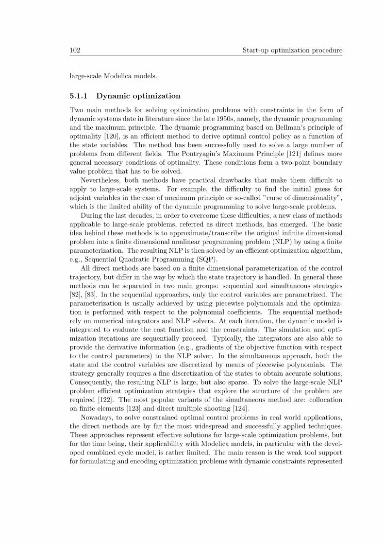
102 Start-up optimization procedure
large-scale Modelica models.
5.1.1 Dynamic optimization
Two main methods for solving optimization problems with constraints in the form ofdynamic systems date in literature since the late 1950s, namely, the dynamic programmingand the maximum principle. The dynamic programming based on Bellman’s principle ofoptimality [120], is an efficient method to derive optimal control policy as a function ofthe state variables. The method has been successfully used to solve a large number ofproblems from different fields. The Pontryagin’s Maximum Principle [121] defines moregeneral necessary conditions of optimality. These conditions form a two-point boundaryvalue problem that has to be solved.
Nevertheless, both methods have practical drawbacks that make them difficult toapply to large-scale systems. For example, the difficulty to find the initial guess foradjoint variables in the case of maximum principle or so-called ”curse of dimensionality”,which is the limited ability of the dynamic programming to solve large-scale problems.
During the last decades, in order to overcome these difficulties, a new class of methodsapplicable to large-scale problems, referred as direct methods, has emerged. The basicidea behind these methods is to approximate/transcribe the original infinite dimensionalproblem into a finite dimensional nonlinear programming problem (NLP) by using a finiteparameterization. The resulting NLP is then solved by an efficient optimization algorithm,e.g., Sequential Quadratic Programming (SQP).
All direct methods are based on a finite dimensional parameterization of the controltrajectory, but differ in the way by which the state trajectory is handled. In general thesemethods can be separated in two main groups: sequential and simultaneous strategies[82], [83]. In the sequential approaches, only the control variables are parametrized. Theparameterization is usually achieved by using piecewise polynomials and the optimiza-tion is performed with respect to the polynomial coefficients. The sequential methodsrely on numerical integrators and NLP solvers. At each iteration, the dynamic model isintegrated to evaluate the cost function and the constraints. The simulation and opti-mization iterations are sequentially proceed. Typically, the integrators are also able toprovide the derivative information (e.g., gradients of the objective function with respectto the control parameters) to the NLP solver. In the simultaneous approach, both thestate and the control variables are discretized by means of piecewise polynomials. Thestrategy generally requires a fine discretization of the states to obtain accurate solutions.Consequently, the resulting NLP is large, but also sparse. To solve the large-scale NLPproblem efficient optimization strategies that explore the structure of the problem arerequired [122]. The most popular variants of the simultaneous method are: collocationon finite elements [123] and direct multiple shooting [124].
Nowadays, to solve constrained optimal control problems in real world applications,the direct methods are by far the most widespread and successfully applied techniques.These approaches represent effective solutions for large-scale optimization problems, butfor the time being, their applicability with Modelica models, in particular with the devel-oped combined cycle model, is rather limited. The main reason is the weak tool supportfor formulating and encoding optimization problems with dynamic constraints represented
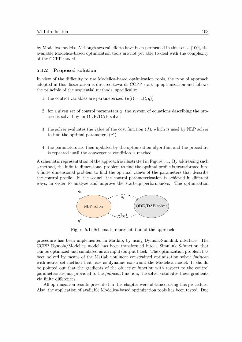
5.1 Introduction 103
by Modelica models. Although several efforts have been performed in this sense [100], theavailable Modelica-based optimization tools are not yet able to deal with the complexityof the CCPP model.
5.1.2 Proposed solution
In view of the difficulty to use Modelica-based optimization tools, the type of approachadopted in this dissertation is directed towards CCPP start-up optimization and followsthe principle of the sequential methods, specifically:
1. the control variables are parameterized (u(t) = u(t, q))
2. for a given set of control parameters q0 the system of equations describing the pro-cess is solved by an ODE/DAE solver
3. the solver evaluates the value of the cost function (J), which is used by NLP solverto find the optimal parameters (q∗)
4. the parameters are then updated by the optimization algorithm and the procedureis repeated until the convergence condition is reached
A schematic representation of the approach is illustrated in Figure 5.1. By addressing sucha method, the infinite dimensional problem to find the optimal profile is transformed intoa finite dimensional problem to find the optimal values of the parameters that describethe control profile. In the sequel, the control parameterization is achieved in differentways, in order to analyze and improve the start-up performances. The optimization
NLP solver ODE/DAE solver
q0
q∗J(qi)
qi
Figure 5.1: Schematic representation of the approach
procedure has been implemented in Matlab, by using Dymola-Simulink interface. TheCCPP Dymola/Modelica model has been transformed into a Simulink S-function thatcan be optimized and simulated as an input/output block. The optimization problem hasbeen solved by means of the Matlab nonlinear constrained optimization solver fminconwith active set method that uses as dynamic constraint the Modelica model. It shouldbe pointed out that the gradients of the objective function with respect to the controlparameters are not provided to the fmincon function, the solver estimates these gradientsvia finite differences.
All optimization results presented in this chapter were obtained using this procedure.Also, the application of available Modelica-based optimization tools has been tested. Due
104 Start-up optimization procedure
to the complexity of the process representation, the existing tools have proved unable tohandle the entire structure of the derived CCPP model. However, for a comparative idea,optimization problems based on subsystems of the CCPP model have been formulatedand solved using the proposed procedure and the platform JModelica.org for optimizationof Modelica models [100]. JModelica.org provides efficient algorithms for solving dynamicoptimization problems (e.g., algorithms based on the direct collocation method with theinterior point optimization solver, IPOPT [125]).
Remark 5.1.1. The optimization methods often require feasible initial values in orderto ensure robust convergence. The initial values of the parameters in the optimizationprocedure have been derived from the profile corresponding to a classical start-up sequenceapplied on the CCPP model.
5.2 Open-loop trajectory optimization
In general the traditional CCPP start-up sequence is quite conservative since in order toguarantee the safety and the availability of the operations, it imposes a series of limitationson the main control variables (e.g., on GT load rate). This type of sequence limitsnaturally the stress in thick components. In fact, the classical strategy is focused mainlyon safety and availability rather than on efficiency of the operation. A new approach forthe CCPP start-up process is proposed in this section, the idea is to implement a moreflexible start-up strategy that eliminates as much as possible these limitations, withoutcompromising the safe operation and keeping the lifetime consumption of the most stressedcomponents under control.
The approach aims at deriving an optimal profile of the plant control variables (e.g.,GT load, ST throttle valve position, DSH flow rate), by assuming that this profile can bedescribed by a parameterized function. The parameters of this function are computed bysolving either a minimum-time optimal control problem or an optimal quadratic trackingproblem, subject to the plant dynamics and to constraints on the main plant variables,such as pressures, temperatures and stresses.
CCPP start-up is a complex task which includes different phases, involving severalinterconnected subsystems. In general, the optimization of the entire sequence requiresconsideration of a hybrid system in which discrete and continuous variables interact. Toreduce the complexity of optimization problem of the whole start-up process, the entireproblem can be decomposed into simpler sub-problems corresponding to each start-upphase. The idea is to divide the start-up sequence in successive steps which are separatelyoptimized, by performing a phase by phase optimization.
Since the most critical part of the start-up sequence in terms of lifetime consumption(the peak values of stress are reached) involves the ST operation, the optimization problemformulation is focused on the last stage of the sequence, namely, the part after the startingof the steam admission in the ST. The applicability of the approach can be easily extendedto other start-up phases.
The optimization procedure can be used to find an optimal trajectory for differentsystem control variables (GT load, bypass, ST throttle, DSH water flow rate, etc.), but

5.2 Open-loop trajectory optimization 105
as the variable that induces most of the dynamic characteristics during the start-up pro-cedure is the GT load, in particular in the last part of the sequence, it will represent thevariable of interest for optimization. Besides the profile optimization of the GT load fora reduction of the start-up time, another study is also performed on the ST throttle fora better control of the thermo-mechanical rotor stress.
5.2.1 Gas Turbine load profile optimization
The goal of the optimization problem is mainly to find the GT load profile that mini-mizes the time required to reach the final point of the start-up (full load conditions) whilefulfilling constraints on the process variables; typically, it is required that temperatures,pressures and stresses remain into specified limits for safety and availability of the oper-ation. The posed problem corresponds to a minimum-time optimal control problem thatwill be presented below.
Another aspect derived from practice, where in order to provide electricity in timea planning of the plant operation is carried out, the start-up problem can be stated asan optimal quadratic tracking problem subject to constraints. In this type of problemthe optimization horizon is fixed a priori, the objective being to reach the final point ofthe start-up (availability of the nominal operation) at the indicated time (”just-in-time”optimization problem).
5.2.1.1 Problem formulation
Start-up minimum-time problem
Consider that the CCPP nonlinear model developed in the previous chapter can be giveninto a dynamic explicit form:
x(t) = f(x(t), z(t), u(t), L(t), t, p)
0 = g(x(t), z(t), u(t), L(t), t, p)(5.1)
where x(t) is the differential state profile vectors (temperatures, pressures, enthalpies,etc.), z(t) denotes algebraic state profile vectors, u(t) is the vector of input profiles whichare not concerned by the optimization procedure (e.g., feed flow to the desuperheater,bypass valve, etc.), L(t) represents the GT load profile (the control profile to optimize)and p is a time-independent parameter vector.
Let t0 and tf denote the initial time instant of the start-up procedure (conventionallylet t0 = 0) and the final time, respectively. Also considering the start-up conditions, forthe load profile the following values are selected: L(t0) = Lm and L(tf ) = LM , where Lm
and LM are the initial and final (full) loads.
Assumption 5.2.1. The control variable profile can be described by a parameterizedfunction, L(t, q), satisfying the boundary conditions stated above, with q a vector ofunknown parameters that have to be derived through an optimization procedure.
106 Start-up optimization procedure
The optimal GT load profile determination consists in finding the value of the pa-rameters vector, q, together with the final start-up time, tf , as solutions of the followingoptimization problem:
minq,tf
(J =
∫ tf
t0
dt) (5.2)
subject to the constraints
x(t) = f(x(t), z(t), u(t), L(t, q), t, p)
0 = g(x(t), z(t), u(t), L(t, q), t, p)(5.3)
L(tf , q) ≥ LM − ǫ1 (5.4)
|f(x(tf ), u(tf ), z(tf ), L(tf , q)| ≤ ǫ2 (5.5)
c(x(t)) ≤ 0, t0 ≤ t ≤ tf (5.6)
where ǫ1 and ǫ2 are tightening terms of the constraints (ideally equal to zero) and thecorresponding constraints are included to guarantee that at the final time tf the systemhas reached the full load with an error specified by ǫ1 (5.4) and is in stationary conditionswith an error specified by ǫ2 (5.5). The last constraint (5.6) includes, in a general form,all the constraints to be imposed on the plant variables during the start-up procedure.In the following, the main operational constraints included in the optimization procedureare on the level of stress in the critical components, namely, the superheater outlet header(5.6a) and the ST rotor (5.6b). It should be stated that additional constraints on theplant variables can be included (e.g., GT load rate of change, required power production,variation rate of the stress level, drum level), thus according to the intended objectivesthe procedure can be easily modified.
σSH(t) ≤ σmaxSH (5.6a)
σST (t) ≤ σmaxST (5.6b)
where σSH and σST are the equivalent stresses on the header and on the external surfaceof the rotor; σmax
SH and σmaxST are the peak values corresponding to admissible stresses on
the header and on the rotor surface, respectively.
Start-up ”just-in-time” optimization problem
Considering the dynamic system representation (5.1) and the same start-up conditionsas in the previous minimum time problem, the optimal GT load profile is determined byfinding the value of the parameters vector, q, as solution of the following optimizationproblem:
minq
(J =
∫ tf
t0
(L(t, q)− LM )2dt) (5.7)

5.2 Open-loop trajectory optimization 107
subject to the constraints (5.3) to (5.6). In this case an integral square error criterion(ISE) is used in order to drive the system towards the desired set point (L(t, q) = LM ) inthe interval [t0, tf ], where the final start-up time, tf is not an optimization parameters,being fixed a priori.
5.2.1.2 Parameterized functions
The variety of functions that can be selected to describe the GT load profile is quite wide.Based on the experience of the operators and analyzing the GT load transient duringa standard start-up procedure, the GT load profile can be associated with a sigmoidfunction. In fact, the selection of the functions is important, because, as it will be seen inthe following sections, the performed choice can lead to a more or less suboptimal solutionof the original problem.
In the sequel, several types of functions have been considered, e.g., Hill functions,or a more general situation by using special functions defined piecewise by polynomi-als, in order to derive the optimal profile with the best compromise between executiontime/convergence and start-up performance.
5.2.1.2.1 Parameterization based on Hill function
Hill function
A first choice is to describe the GT load profile as a Hill function:
L(t, q) = Lm + (LM − Lm)th
th + kh(5.8)
where q = [h, k] is the parameter vector to be determined through optimization. Consid-ering an example with the following start-up conditions, Lm = 0, LM = 1, t0 = 0 andtf = 5000 [s], the graphical representation of the Hill function for different values of theparameters is shown in Figure 5.2a.
2-Hill function
The GT load profile can be also represented by connecting two or more Hill functions (orequivalent) in cascade. The representation of the GT load as a combination of two Hillfunctions is formulated as follows:
L(t, q) = Lm + (Li − Lm)th
th + kh+ (LM − Li)
tp
tp + rp(5.9)
where q = [h, k, p, r, Li] is the parameter vector to be determined through the optimiza-tion procedure. The graphical representation of the function for different values of theparameters, considering the same start-up conditions as in the previous case, is shown inFigure 5.2b.
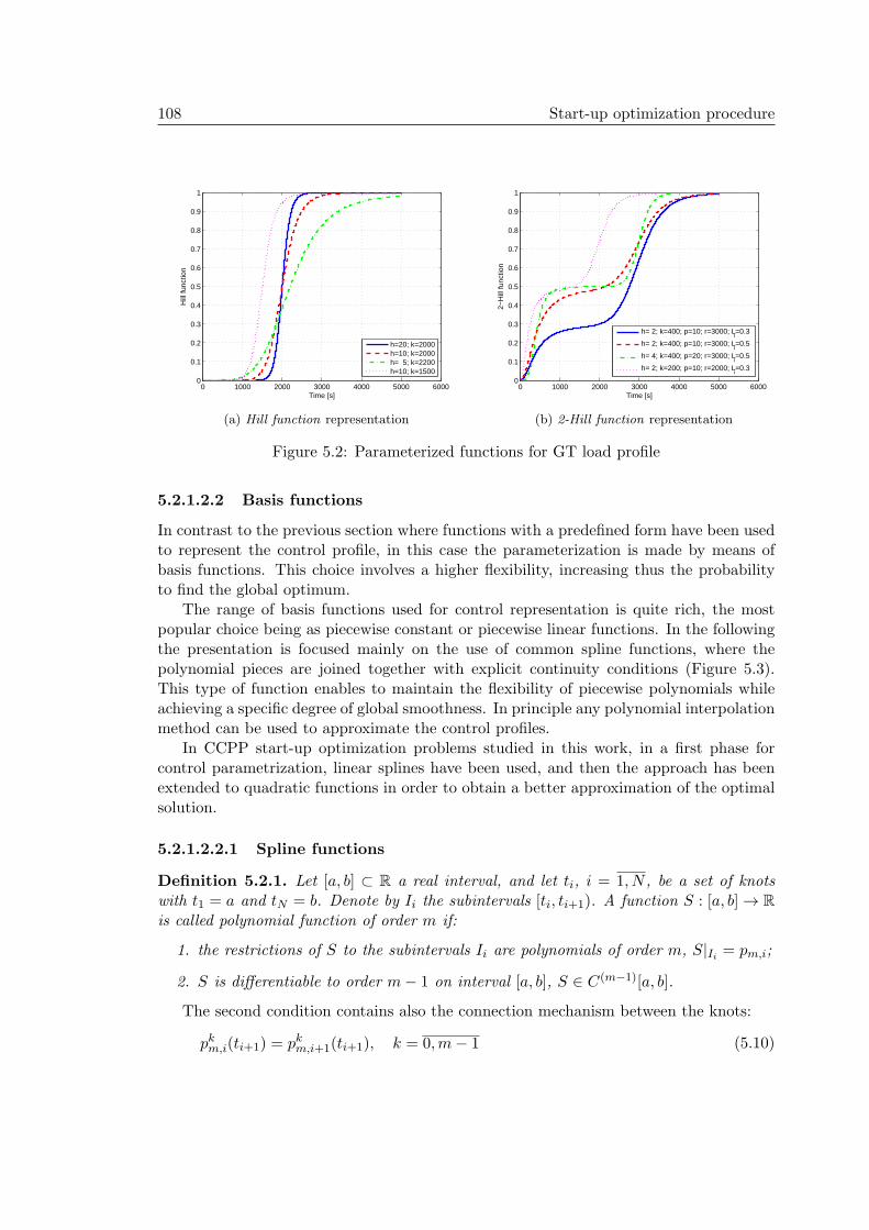
108 Start-up optimization procedure
0 1000 2000 3000 4000 5000 60000
0.1
0.2
0.3
0.4
0.5
0.6
0.7
0.8
0.9
1
Time [s]
Hill
func
tion
h=20; k=2000h=10; k=2000h= 5; k=2200h=10; k=1500
(a) Hill function representation
0 1000 2000 3000 4000 5000 60000
0.1
0.2
0.3
0.4
0.5
0.6
0.7
0.8
0.9
1
Time [s]
2−H
ill fu
nctio
n
h= 2; k=400; p=10; r=3000; Li=0.3
h= 2; k=400; p=10; r=3000; Li=0.5
h= 4; k=400; p=20; r=3000; Li=0.5
h= 2; k=200; p=10; r=2000; Li=0.3
(b) 2-Hill function representation
Figure 5.2: Parameterized functions for GT load profile
5.2.1.2.2 Basis functions
In contrast to the previous section where functions with a predefined form have been usedto represent the control profile, in this case the parameterization is made by means ofbasis functions. This choice involves a higher flexibility, increasing thus the probabilityto find the global optimum.
The range of basis functions used for control representation is quite rich, the mostpopular choice being as piecewise constant or piecewise linear functions. In the followingthe presentation is focused mainly on the use of common spline functions, where thepolynomial pieces are joined together with explicit continuity conditions (Figure 5.3).This type of function enables to maintain the flexibility of piecewise polynomials whileachieving a specific degree of global smoothness. In principle any polynomial interpolationmethod can be used to approximate the control profiles.
In CCPP start-up optimization problems studied in this work, in a first phase forcontrol parametrization, linear splines have been used, and then the approach has beenextended to quadratic functions in order to obtain a better approximation of the optimalsolution.
5.2.1.2.2.1 Spline functions
Definition 5.2.1. Let [a, b] ⊂ R a real interval, and let ti, i = 1, N , be a set of knotswith t1 = a and tN = b. Denote by Ii the subintervals [ti, ti+1). A function S : [a, b] → R
is called polynomial function of order m if:
1. the restrictions of S to the subintervals Ii are polynomials of order m, S|Ii = pm,i;
2. S is differentiable to order m− 1 on interval [a, b], S ∈ C(m−1)[a, b].
The second condition contains also the connection mechanism between the knots:
pkm,i(ti+1) = pkm,i+1(ti+1), k = 0,m− 1 (5.10)
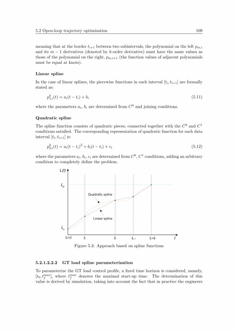
5.2 Open-loop trajectory optimization 109
meaning that at the border ti+1 between two subintervals, the polynomial on the left pm,i
and its m − 1 derivatives (denoted by k-order derivative) must have the same values asthose of the polynomial on the right, pm,i+1 (the function values of adjacent polynomialsmust be equal at knots).
Linear spline
In the case of linear splines, the piecewise functions in each interval [ti, ti+1] are formallystated as:
pk1,i(t) = ai(t− ti) + bi (5.11)
where the parameters ai, bi are determined from C0 and joining conditions.
Quadratic spline
The spline function consists of quadratic pieces, connected together with the C0 and C1
conditions satisfied. The corresponding representation of quadratic function for each datainterval [ti, ti+1] is:
pk2,i(t) = ai(t− ti)2 + bi(t− ti) + ci (5.12)
where the parameters ai, bi, ci are determined from C0, C1 conditions, adding an arbitrarycondition to completely define the problem.
Quadratic spline
Linear spline
t0=0
L(t)
t1 tk tn-1 t tn f= t
LM
Lm
Figure 5.3: Approach based on spline functions
5.2.1.2.2.2 GT load spline parameterization
To parameterize the GT load control profile, a fixed time horizon is considered, namely,[t0, t
maxf ], where tmax
f denotes the maximal start-up time. The determination of thisvalue is derived by simulation, taking into account the fact that in practice the engineers
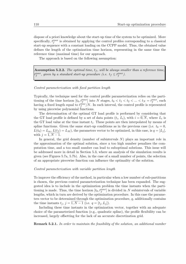
110 Start-up optimization procedure
dispose of a priori knowledge about the start-up time of the system to be optimized. Morespecifically, tmax
f is obtained by applying the control profiles corresponding to a classicalstart-up sequence with a constant loading on the CCPP model. Thus, the obtained valuedefines the length of the optimization time horizon, representing in the same time thereference time (maximal time) for our approach.
The approach is based on the following assumption:
Assumption 5.2.2. The optimal time, tf , will be always smaller than a reference time,tmaxf , given by a standard start-up procedure (i.e. tf ≤ tmax
f ).
Control parameterization with fixed partition length
Typically, the technique used for the control profile parameterization relies on the parti-tioning of the time horizon [t0, t
maxf ] into N stages, t0 < t1 < t2 < ... < tN = tmax
f , eachhaving a fixed length equal to tmax
f /N . In each interval, the control profile is representedby using piecewise polynomial functions.
The determination of the optimal GT load profile is performed by considering thatthe GT load profile is defined by a set of data points (ti, Li), with i = 0, N , where Li isthe GT load value at the time instant ti. These points are then interpolated by means ofspline functions. Given the same start-up conditions as in the previous case (i.e. t0 = 0,L(t0) = Lm, L(tf ) = LM ), the parameters vector to be optimized, in this case, is q = [Lj ],with j = 1, N − 1.
In general, the grid density (number of subintervals N) plays an important role inthe approximation of the optimal solution, since a too high number penalizes the com-putation time, and a too small number can lead to suboptimal solutions. This issue willbe addressed more in detail in Section 5.3, where an analysis of the simulation results isgiven (see Figures 5.7a, 5.7b). Also, in the case of a small number of points, the selectionof an appropriate piecewise function can influence the optimality of the solution.
Control parameterization with variable partition length
To improve the efficiency of the method, in particular when a low number of sub-partitionsis chosen, the previous control parameterization technique has been expanded. The sug-gested idea is to include in the optimization problem the time instants when the parti-tioning is made. Thus, the time horizon [t0, t
maxf ] is divided in N subintervals of variable
lengths, which in turn are derived by the optimization procedure. In this case the parame-ters vector to be determined through the optimization procedure, q, additionally containsthe time instants tj , j = 1, N − 1 (i.e. q = [tj , Lj ]).
Including these time instants in the optimization vector, together with an adequatechoice of the parameterized function (e.g., quadratic spline), the profile flexibility can beincreased, largely offsetting for the lack of an accurate discretization grid.
Remark 5.2.1. In order to maintain the feasibility of the solution, an additional number

5.2 Open-loop trajectory optimization 111
of linear constraints on the parameters bounds have been imposed:
Lm ≤ L(t, q) ≤ LM (5.13)
so that the GT load remains between the minimal and maximal load. In addition for thesecond case:
t0 ≤ tj ≤ tf , j = 1, N − 1 (5.14)
so that the parameters remain in the feasible domain.
5.2.2 GT load profile and ST throttle opening profile optimization
In the procedure outlined above, only the GT load has been used as optimization variable,the other control inputs of the system being considered as constants (e.g., DSH water flowrate), or represented as a predefined function of the GT load (e.g., ST throttle valve).In order to improve the start-up performances even further, the procedure can be easilyextended to aim also other inputs, for example, in this section the ST throttle opening isincluded in the optimization procedure.
Problem formulation
Let Assumption 5.2.1 hold for ST throttle valve. The ST valve opening profile is rep-resented by using a parameterized function (Ot(t, v)), where v denotes the parametersvector. The start-up conditions are specified by O(t0) = Om and O(tf ) = OM , whereOm, OM are the initial and final opening values. The optimization procedure follows thesame principle as in previous case; the optimal profiles of the GT load and ST throttleare determined by solving a minimum time problem:
minq,v,tf
(J =
∫ tf
t0
dt) (5.15)
subject to the constraints (5.4) to (5.6)
x(t) = f(x(t), z(t), u(t), L(t, q), Ot(t, v), t, p)
0 = g(x(t), z(t), u(t), L(t, q), Ot(t, v), t, p)(5.16)
O(tf , v) ≥ OM − ǫv (5.17)
where ǫv denotes tightening term of the constraint (ideally equal to zero) and the corre-sponding constraint (5.17), is included to ensure that at the final start-up time tf the STvalve is (almost) completely open.
In this case the overall parameter vector to be optimized contains the parametersthat describe the GT load profile (q) and the parameters of the ST throttle profile (v)respectively. Similar to the parameters vector q, v can contain the set of data points usedby the spline functions or the parameters of the Hill functions.

112 Start-up optimization procedure
5.3 Results
The approach presented in the previous section has been applied to a hot part of thestart-up sequence. The part corresponds to the last stage of the sequence, after the steamadmission begins and ST is synchronized to the grid (see also Section 2.2.5.6). Namely,the initial conditions of the model assumed in this case correspond to:
• the bypass valve is closed;
• the ST is synchronized and connected to grid;
• the feed-water flow rate is of approximatively 19 kg/s;
• the DSH feed-water flow rate is set at nominal value (0);
• the throttle valve is set to a value that ensures a pressure in circuit of 60 bar;
• the load of the GT is set to 15% (Lm = 0.15).
It should be noted that, regarding the ST valve, a loop that controls its position tomaintain the pressure in circuit at a specified value (i.e. 60 bar) is used. The controlloop is active only when the GT load is below 50%, above this value the opening directlydepends on the GT load (sliding pressure mode).
The concerned stage of the start-up is considered as one of the most critical regardingthe lifetime consumption of the system components. The optimization procedure has beenimplemented by imposing a number of constraints on the main plant variables, in order toprevent any possible unsafe conditions and to preserve the life of the units. In particular,the constraints are imposed on the maximum values of thermal-mechanical stresses in themost affected components, namely, the rotor and the superheater outlet header. Thesepeaks determine in general the lifetime consumption during the entire start-up (i.e. thecreep phenomenon depends mainly on the temporal peak stress), without consideringadditional effects caused by the variation rate of the stress level (i.e. the fatigue crackdue to fluctuating stress). The peak values for the header stress and the rotor stress havebeen fixed to not exceed 116 MPa and 460 MPa, respectively (5.18c). These limits areconsistent with typical values estimated on a real plant during the start-up phase andcorrespond to a normal start-up procedure.
As already stated, the objective of the optimization problem is to reach the finalpoint of the start-up as fast as possible, while keeping the lifetime consumption of themost stressed components under control. The start-up sequence is considered as beingcompleted when the GT load exceeds 99.3% (ǫ1 = 0.7%) and the stationary conditionsare reached with ǫ2 = 1%, meaning that the gradient of the steam temperature is lowerthan 0.01 K/s and the pressure gradient is below 0.01 bar/s (5.18a-5.18b).
L(tf , q) ≥ 0.993 (5.18a)
Ts(tf ) ≤ 0.01 K/s
ps(tf ) ≤ 1000 Pa/s(5.18b)

5.3 Results 113
σSH(t) ≤ 116 MPa
σST (t) ≤ 460 MPa(5.18c)
5.3.1 Comparison standard sequence - optimal procedure for minimal
start-up time
In order to show the advantages of the proposed approach, based on the above initialconditions, a comparison between the performances in terms of start-up time and con-sumption of the optimal procedure with respect to a standard start-up sequence has beenperformed. The classical start-up procedure uses a conservative load rate limit to takeinto consideration the worst case plant conditions. Thus in our case, during the lastpart of the sequence the considered GT load ramp has a slope limited to 2 MW/min.This value corresponds to the constant GT load rate that ensures the fulfillment of theconstraints imposed on the stress.
5.3.1.1 Hill functions vs. classical profile
Assuming that GT load profile is described as a Hill function, the optimization procedurehas been implemented, resulting in the GT load optimal profile shown in Figure 5.4a. As
0 2000 4000 6000 8000 10000 12000 14000 160000.1
0.2
0.3
0.4
0.5
0.6
0.7
0.8
0.9
1
Time [s]
GT
Loa
d [n
orm
aliz
ed]
GT load profile − Hill function
(a) GT Load profile described as a Hill function
0 1000 2000 3000 4000 5000 60000.1
0.2
0.3
0.4
0.5
0.6
0.7
0.8
0.9
1
Time [s]
GT
Loa
d [n
orm
aliz
ed]
GT Load − standard start−upGT Load − 2−Hill functions
(b) Standard and optimal GT Load profile
Figure 5.4: Start-up with an optimal profile based on Hill functions vs. standard proce-dure
it can be seen, by using this type of functions, the optimization procedure can guaranteea safe operation (see Figure 5.5) but with a very suboptimal solution in terms of start-uptime. Nevertheless, this simple choice to describe the input signal could be useful tooptimize other start-up phases (e.g., HRSG Start-up phase), or for the concerned phase,by connecting two such functions in cascade. Thus, considering that the load profile isdescribed by a 2-Hill function, the start-up time can be significantly reduced with respectto the standard procedure (see Figure 5.4b).

114 Start-up optimization procedure
0 2000 4000 6000 8000 10000 12000 14000 1600050
60
70
80
90
100
110
120
Time [s]
Hea
der
stre
ss [M
Pa]
Header stress − GT Loadas optimal Hill function
(a) Header stress evaluation
0 2000 4000 6000 8000 10000 12000 14000 160000
50
100
150
200
250
300
350
400
450
500
Time [s]
Rot
or s
tres
s [M
Pa]
Rotor stress − GT Loadas optimal Hill function
(b) Rotor stress evaluation
Figure 5.5: Stress evolution according to GT load profile based on Hill function
The optimization results show that the new procedure based on 2-Hill function isable to reduce the start-up time compared to the classical one by approximately 26% (26minutes), while limiting the peak stress value on the header (Figure 5.6a) and on therotor surface (see Figure 5.6b). An optimization procedure relied on these functions canguarantee a fast and safe start-up operation.
0 1000 2000 3000 4000 5000 600040
50
60
70
80
90
100
110
120
Time [s]
Hea
der
stre
ss [M
Pa]
standard start−upoptimal start−up with 2−Hill functions
(a) Header stress evaluation
0 1000 2000 3000 4000 5000 60000
50
100
150
200
250
300
350
400
450
500
Time [s]
Rot
or s
tres
s [M
Pa]
standard start−upoptimal start−up with 2−Hill functions
(b) Rotor stress evaluation
Figure 5.6: Stress evolution corresponding to the standard GT load profile and optimalprofile based on 2-Hill function
It should be noted that the simple selection of 2-Hill function demonstrates adequateresults for the last stage of start-up. However different input functions can be selected toimprove further the start-up performances, taking into account the fact that a compromisebetween the start-up time performance and the complexity of the optimization, mainlylinked to the number of parameters that define the function, has to be made.
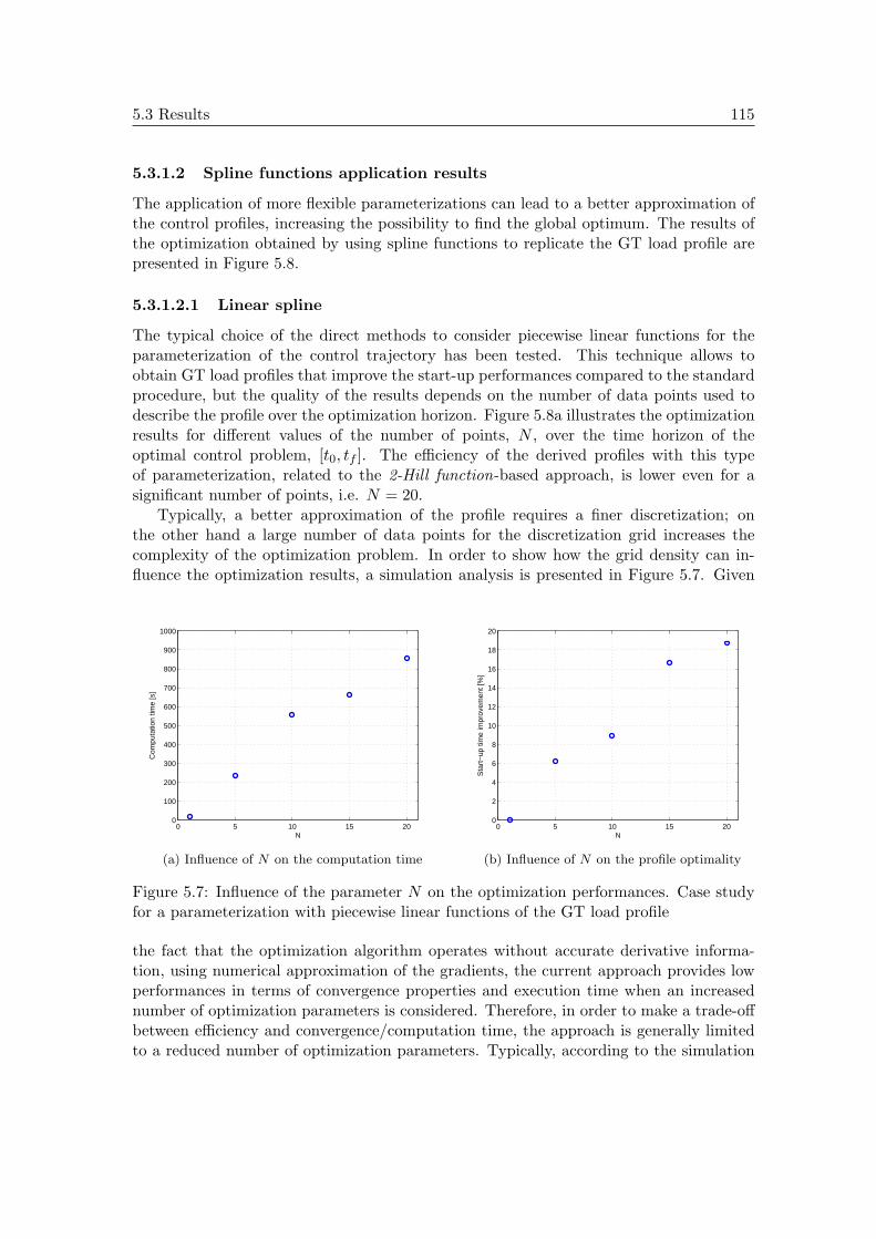
5.3 Results 115
5.3.1.2 Spline functions application results
The application of more flexible parameterizations can lead to a better approximation ofthe control profiles, increasing the possibility to find the global optimum. The results ofthe optimization obtained by using spline functions to replicate the GT load profile arepresented in Figure 5.8.
5.3.1.2.1 Linear spline
The typical choice of the direct methods to consider piecewise linear functions for theparameterization of the control trajectory has been tested. This technique allows toobtain GT load profiles that improve the start-up performances compared to the standardprocedure, but the quality of the results depends on the number of data points used todescribe the profile over the optimization horizon. Figure 5.8a illustrates the optimizationresults for different values of the number of points, N , over the time horizon of theoptimal control problem, [t0, tf ]. The efficiency of the derived profiles with this typeof parameterization, related to the 2-Hill function-based approach, is lower even for asignificant number of points, i.e. N = 20.
Typically, a better approximation of the profile requires a finer discretization; onthe other hand a large number of data points for the discretization grid increases thecomplexity of the optimization problem. In order to show how the grid density can in-fluence the optimization results, a simulation analysis is presented in Figure 5.7. Given
0 5 10 15 200
100
200
300
400
500
600
700
800
900
1000
Com
puta
tion
time
[s]
N
(a) Influence of N on the computation time
0 5 10 15 200
2
4
6
8
10
12
14
16
18
20
Sta
rt−
up ti
me
impr
ovem
ent [
%]
N
(b) Influence of N on the profile optimality
Figure 5.7: Influence of the parameter N on the optimization performances. Case studyfor a parameterization with piecewise linear functions of the GT load profile
the fact that the optimization algorithm operates without accurate derivative informa-tion, using numerical approximation of the gradients, the current approach provides lowperformances in terms of convergence properties and execution time when an increasednumber of optimization parameters is considered. Therefore, in order to make a trade-offbetween efficiency and convergence/computation time, the approach is generally limitedto a reduced number of optimization parameters. Typically, according to the simulation
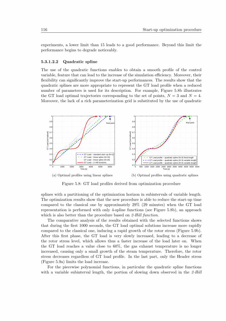
116 Start-up optimization procedure
experiments, a lower limit than 15 leads to a good performance. Beyond this limit theperformance begins to degrade noticeably.
5.3.1.2.2 Quadratic spline
The use of the quadratic functions enables to obtain a smooth profile of the controlvariable, feature that can lead to the increase of the simulation efficiency. Moreover, theirflexibility can significantly improve the start-up performances. The results show that thequadratic splines are more appropriate to represent the GT load profile when a reducednumber of parameters is used for its description. For example, Figure 5.8b illustratesthe GT load optimal trajectories corresponding to the set of points, N = 3 and N = 4.Moreover, the lack of a rich parameterization grid is substituted by the use of quadratic
0 1000 2000 3000 4000 5000 60000.1
0.2
0.3
0.4
0.5
0.6
0.7
0.8
0.9
1
Time [s]
GT
Loa
d [n
orm
aliz
ed]
GT Load − standard start−up (N=1)GT Load − linear spline (N=10)GT Load − linear spline (N=20)GT Load − 2−Hill functions
final point
(a) Optimal profiles using linear splines
0 500 1000 1500 2000 2500 3000 3500 4000 4500 5000 55000.1
0.2
0.3
0.4
0.5
0.6
0.7
0.8
0.9
1
Time [s]
GT
Loa
d [n
orm
aliz
ed]
GT Load profile − quadratic spline (N=3) fixed lengthGT Load profile − quadratic spline (N=3) variable lengthGT Load profile − quadratic spline (N=4) variable length
final point
(b) Optimal profiles using quadratic splines
Figure 5.8: GT load profiles derived from optimization procedure
splines with a partitioning of the optimization horizon in subintervals of variable length.The optimization results show that the new procedure is able to reduce the start-up timecompared to the classical one by approximately 29% (29 minutes) when the GT loadrepresentation is performed with only 4-spline functions (see Figure 5.8b), an approachwhich is also better than the procedure based on 2-Hill function.
The comparative analysis of the results obtained with the selected functions showsthat during the first 1000 seconds, the GT load optimal solutions increase more rapidlycompared to the classical one, inducing a rapid growth of the rotor stress (Figure 5.9b).After this first phase, the GT load is very slowly increased, leading to a decrease ofthe rotor stress level, which allows thus a faster increase of the load later on. Whenthe GT load reaches a value close to 60%, the gas exhaust temperature is no longerincreased, causing only a small growth of the steam temperature. Therefore, the rotorstress decreases regardless of GT load profile. In the last part, only the Header stress(Figure 5.9a) limits the load increase.
For the piecewise polynomial functions, in particular the quadratic spline functionswith a variable subinterval length, the portion of slowing down observed in the 2-Hill
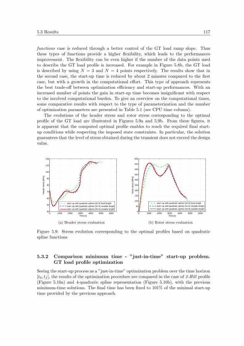
5.3 Results 117
functions case is reduced through a better control of the GT load ramp slope. Thusthese types of functions provide a higher flexibility, which leads to the performancesimprovement. The flexibility can be even higher if the number of the data points usedto describe the GT load profile is increased. For example in Figure 5.8b, the GT loadis described by using N = 3 and N = 4 points respectively. The results show that inthe second case, the start-up time is reduced by about 2 minutes compared to the firstcase, but with a growth in the computational effort. This type of approach representsthe best trade-off between optimization efficiency and start-up performances. With anincreased number of points the gain in start-up time becomes insignificant with respectto the involved computational burden. To give an overview on the computational times,some comparative results with respect to the type of parameterization and the numberof optimization parameters are presented in Table 5.1 (see CPU time column).
The evolutions of the header stress and rotor stress corresponding to the optimalprofile of the GT load are illustrated in Figures 5.9a and 5.9b. From these figures, itis apparent that the computed optimal profile enables to reach the required final start-up conditions while respecting the imposed state constraints. In particular, the solutionguarantees that the level of stress obtained during the transient does not exceed the designvalue.
0 1000 2000 3000 4000 5000 600040
50
60
70
80
90
100
110
120
Time [s]
Hea
der
stre
ss [M
Pa]
start−up with quadratic splines (N=3) fixed lengthstart−up with quadratic splines (N=3) variable lengthstart−up with quadratic splines (N=4) variable length
(a) Header stress evaluation
0 1000 2000 3000 4000 5000 60000
50
100
150
200
250
300
350
400
450
500
Time [s]
Rot
or s
tres
s [M
Pa]
start−up with quadratic splines (N=3) fixed lengthstart−up with quadratic splines (N=3) variable lengthstart−up with quadratic splines (N=4) variable length
(b) Rotor stress evaluation
Figure 5.9: Stress evolution corresponding to the optimal profiles based on quadraticspline functions
5.3.2 Comparison minimum time - ”just-in-time” start-up problem.
GT load profile optimization
Seeing the start-up process as a ”just-in-time” optimization problem over the time horizon[t0, tf ], the results of the optimization procedure are compared in the case of 2-Hill profile(Figure 5.10a) and 4-quadratic spline representation (Figure 5.10b), with the previousminimum-time solutions. The final time has been fixed to 101% of the minimal start-uptime provided by the previous approach.

118 Start-up optimization procedure
0 1000 2000 3000 4000 50000.1
0.2
0.3
0.4
0.5
0.6
0.7
0.8
0.9
1
Time [s]
GT
Loa
d [n
orm
aliz
ed]
GT Load profile − minimum time approachGT Load profile − "just−in−time" approach
(a) Optimal profiles with 2-Hill function
0 1000 2000 3000 4000 50000.1
0.2
0.3
0.4
0.5
0.6
0.7
0.8
0.9
1
Time [s]
GT
Loa
d [n
orm
aliz
ed]
GT Load profile − minimum time approachGT Load profile − "just−in−time" approach
(b) Optimal profiles with quadratic splines
Figure 5.10: GT load profiles derived from the both optimization procedures
As it can be observed, the approach leads to start-up profiles comparable to theminimum-time solution. Therefore, in the case when a coherent final time is provided,the start-up minimum time problem can be seen as an optimal tracking problem subjectto constraints.
5.3.3 GT load profile and ST throttle opening profile optimization
To improve the start-up performances even further, the optimization procedure has beenextended to aim also the ST throttle opening profile. If in the previous case the STthrottle valve opening has been described as a function of GT load, in this procedurethe profile is represented with quadratic spline functions. The new optimal GT load
0 1000 2000 3000 4000 50000.1
0.2
0.3
0.4
0.5
0.6
0.7
0.8
0.9
1
Time [s]
GT
Loa
d [n
orm
aliz
ed]
1−control optimization2−controls optimization
final point
(a) Optimal GT load profiles
0 1000 2000 3000 4000 50000.2
0.3
0.4
0.5
0.6
0.7
0.8
0.9
1
Time [s]
ST
val
ve o
peni
ng [p
.u.]
ST valve profile as function of GT loadoptimal ST valve profile
(b) ST throttle profile representation
Figure 5.11: Comparison profiles 1-control and 2-controls optimization

5.3 Results 119
profile derived with this procedure as well as the solution found in the case of 1-controloptimization problem are reported in Figure 5.11a. In the both cases the control profileshave been parameterized by using 4-quadratic spline functions. Also, the optimized STthrottle profile represented with 3-quadratic spline functions and the ST valve opening asa predefined function of the GT load level are represented in Figure 5.11b. The results
0 1000 2000 3000 4000 500030
40
50
60
70
80
90
100
110
120
Time [s]
Hea
der
stre
ss [M
Pa]
1−control optimization2−controls optimization
(a) Header stress
0 1000 2000 3000 4000 50000
50
100
150
200
250
300
350
400
450
500
Time [s]
Rot
or s
tres
s [M
Pa]
1−control optimization2−controls optimization
(b) Rotor stress
Figure 5.12: Comparison between 1-control and 2-controls optimization stress results
show that by optimizing the ST valve profile (2-controls optimization) a supplementaryreduction of the start-up time (approximatively 3 minutes) is obtained compared to thesingle-control optimization (see Table 5.1 for a more complete comparison). This can beconsidered as a point of interest for the start-up phase, because in 1-control optimization,the ST throttle behavior has been described as a predefined function of the GT load level,and by optimizing its profile a better control on the ST rotor stress can be performed (seeFigure 5.12b). Nevertheless, the gain in start-up time is not significant compared to theinvolved computation time.
5.3.4 Validation on the reference CCPP model
The different optimal profiles computed with the smooth model have been applied tosimulate the last part of the start-up procedure on the original combined cycle model. Inthis section, as case study only the GT load profile representation with quadratic splinesis considered. The transients of some relevant plant variables corresponding to this profileare illustrated in Figures 5.13 to 5.14.
From the derived results it can be observed that the responses of the two modelsare quite close to each other, validating once again the consistency of the CCPP smoothmodel . Also, the optimal solution found with the smooth model remains valid in thecase of the CCPP reference one, ensuring that the constraints imposed on the main plantsvariables are fulfilled.

120 Start-up optimization procedure
0 1000 2000 3000 4000 5000600
650
700
750
800
850
Time [s]
T [K
]
CCPP smooth modelCCPP reference model
(a) Steam temperature
0 1000 2000 3000 4000 500060
65
70
75
80
85
90
95
100
Time [s]
p [b
ar]
CCPP smooth modelCCPP reference model
(b) Steam pressure
Figure 5.13: Evolution of steam parameters corresponding to the smooth and referencemodel
0 1000 2000 3000 4000 500040
50
60
70
80
90
100
110
120
Time [s]
Hea
der
stre
ss [M
Pa]
CCPP smooth modelCCPP reference model
(a) Header stress
0 1000 2000 3000 4000 50000
50
100
150
200
250
300
350
400
450
500
Time [s]
Rot
or s
tres
s [M
Pa]
CCPP smooth modelCCPP reference model
(b) Rotor stress
Figure 5.14: Evolution of the stress corresponding to the smooth and reference model
5.3.5 Start-up improvement benefits
The main benefit of shortening the start-up time is the reduction of the operating costs.A first gain is due to lower fuel consumption. A comparison between the fuel consumptionfor two optimal profiles, related to the classical start-up, is given in Figure 5.15a. Theresults show that the new optimal start-up procedure consumes up to 36% less than thetraditional start-up.
Also, taking into account the losses during the start-up related to an operation ofthe plant in nominal mode (Figure 5.15b), the reduction of the start-up time involvesconsiderable saved earnings (up to 32%). In Figure 5.15b, the Loss indicates the earningsif the plant would have fictitiously operated at nominal power during a period equivalent

5.3 Results 121
0 1000 2000 3000 4000 5000 60000
0.2
0.4
0.6
0.8
1
1.2
Time [s]
Fue
l con
sum
ptio
n [n
orm
aliz
ed]
standard start−upoptimal start−up with 2−Hill functionstart−up with 2−controls optimization
(a) Fuel consumption comparison
4000 4500 5000 5500 6000 650040
45
50
55
60
65
Start−up time [s]
Loss
[kE
uros
]
standard start−up sequenceoptimal start−up with 2−Hill functionoptimal start−up with 4−quadratic splinesstart−up with 2−controls optimization
(b) Losses reduction comparison
Figure 5.15: Start-up reduction benefits
to the start-up time, defined as:
Loss = En ∗ pe (5.19)
where En denotes the delivered electrical energy (KWh), and pe denotes the tariff (ine/KWh) of the electricity. A complete comparison in terms of benefits, computationtime and number of optimization parameters, between all the profile-functions consideredin this section can be found in Table 5.1. Also in Table 5.1, a ratio between the start-up time gain and complexity, defined as in 5.20, is presented. This ratio quantifies thetrade-off between complexity and performance, showing in some measure the possibilityfor a real-time implementation.
r =gtc
(5.20)
with
gt =tref − tst
tref(5.20a)
c =tc − trctrc
(5.20b)
where tst is the start-up time derived by optimization procedure, tref is the start-up timecorresponding to the standard procedure considered as reference time, tc is the compu-tation time required for the resolution of the optimization problem and trc denotes thecomputation time corresponding the standard start-up considered as reference computa-tion time.
It should be pointed out that the computation time and the convergence propertiesstrongly depend on the initial values of the optimization parameters selected in the pro-cedure. In all these cases a feasible set of initial values derived from the standard start-upprofile has been used.
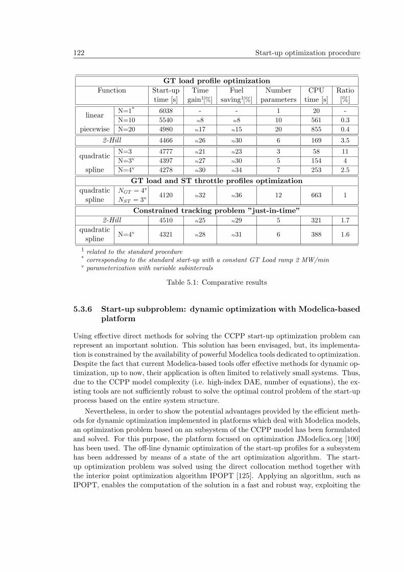
122 Start-up optimization procedure
GT load profile optimization
Function Start-up Time Fuel Number CPU Ratiotime [s] gain1[%] saving1[%] parameters time [s] [%]
linearN=1* 6038 - - 1 20 -N=10 5540 ≈8 ≈8 10 561 0.3
piecewise N=20 4980 ≈17 ≈15 20 855 0.4
2-Hill 4466 ≈26 ≈30 6 169 3.5
quadraticN=3 4777 ≈21 ≈23 3 58 11
N=3v 4397 ≈27 ≈30 5 154 4
spline N=4v 4278 ≈30 ≈34 7 253 2.5
GT load and ST throttle profiles optimization
quadratic NGT = 4v4120 ≈32 ≈36 12 663 1
spline NST = 3v
Constrained tracking problem ”just-in-time”
2-Hill 4510 ≈25 ≈29 5 321 1.7
quadraticN=4v 4321 ≈28 ≈31 6 388 1.6
spline
1 related to the standard procedure* corresponding to the standard start-up with a constant GT Load ramp 2 MW/minv parameterization with variable subintervals
Table 5.1: Comparative results
5.3.6 Start-up subproblem: dynamic optimization with Modelica-based
platform
Using effective direct methods for solving the CCPP start-up optimization problem canrepresent an important solution. This solution has been envisaged, but, its implementa-tion is constrained by the availability of powerful Modelica tools dedicated to optimization.Despite the fact that current Modelica-based tools offer effective methods for dynamic op-timization, up to now, their application is often limited to relatively small systems. Thus,due to the CCPP model complexity (i.e. high-index DAE, number of equations), the ex-isting tools are not sufficiently robust to solve the optimal control problem of the start-upprocess based on the entire system structure.
Nevertheless, in order to show the potential advantages provided by the efficient meth-ods for dynamic optimization implemented in platforms which deal with Modelica models,an optimization problem based on an subsystem of the CCPP model has been formulatedand solved. For this purpose, the platform focused on optimization JModelica.org [100]has been used. The off-line dynamic optimization of the start-up profiles for a subsystemhas been addressed by means of a state of the art optimization algorithm. The start-up optimization problem was solved using the direct collocation method together withthe interior point optimization algorithm IPOPT [125]. Applying an algorithm, such asIPOPT, enables the computation of the solution in a fast and robust way, exploiting the
5.3 Results 123
sparsity structure of the resulting NLP.
5.3.6.1 Subsystem model
The dynamic optimization considered in this section is based on a nonlinear model com-posed of the GT unit and a heat exchanger (economizer). The control input of the sub-system, that will be used as manipulated variable in the start-up optimization problem, isrepresented by the load level of the GT. According to the Dymola’s statistic information,the model is described by a DAE with 481 equations and 12 state variables.
5.3.6.2 Optimization problem
As already stated, the definition of a dynamic optimization problem is an iterative proce-dure. The result of such a procedure in the case of a start-up problem based on a CCPPsubsystem, regarding the adaptation of the model, objectives and constraints definition,is given in a final formulation in this section.
Specifications
As in the case of the start-up optimization procedure already stated, the goal of theoptimization problem formulated in this section is to reach the GT full load level asquickly as possible, while limiting the stress value on the metal surface of the exchanger.The objective is formulated by means of a Lagrange-type cost function, penalizing thesquared deviation from the target value represented by the full load (5.21). The full loadstate is considered when the load level of the GT (L(t)) has reached the final target of100% (LM = 1).
In this case a limiting factor in the start-up problem is the constraint acting on thethermal stress in the heat exchanger (5.22). The thermal stress is kept under control bylimiting the allowable temperature gradient in the metal Tm.
In addition, inequality constraints are imposed on the rate of change of the GT loadprofile. A constraint is imposed so that the GT load must not exceed the maximum rate∆Lmax specified by the manufacturer (5.23), and a constraint is considered to impose apositive gradient in order to avoid as far as possible the multiple cycling of the stress levelduring the transient (5.24).
Optimal control problem
Considering the specifications presented above, the optimization problem has been for-mulated as:
minL(t)
∫ tf
t0
(L(t)− LM )2dt) (5.21)
subject to the constraints
Tm(t) ≤ ∆Tmax (5.22)
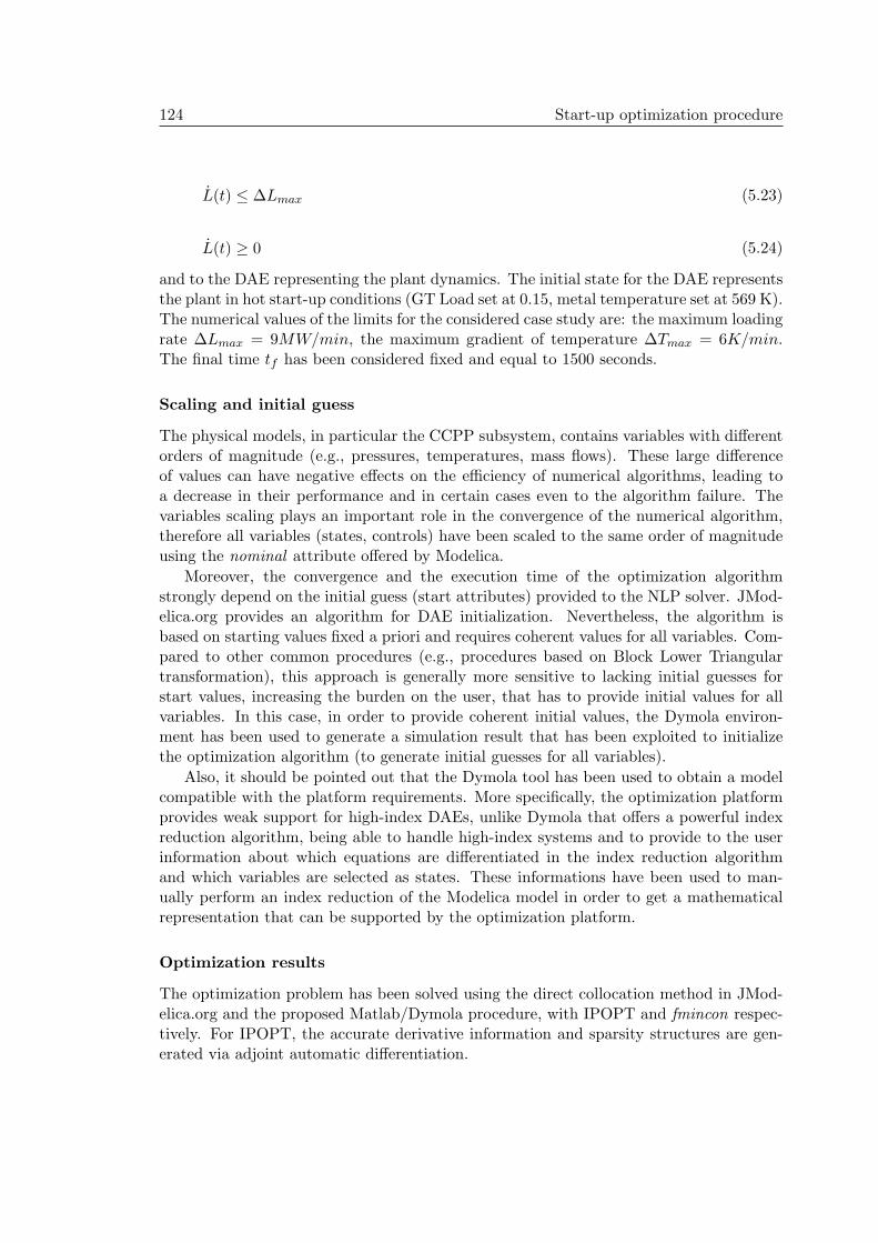
124 Start-up optimization procedure
L(t) ≤ ∆Lmax (5.23)
L(t) ≥ 0 (5.24)
and to the DAE representing the plant dynamics. The initial state for the DAE representsthe plant in hot start-up conditions (GT Load set at 0.15, metal temperature set at 569 K).The numerical values of the limits for the considered case study are: the maximum loadingrate ∆Lmax = 9MW/min, the maximum gradient of temperature ∆Tmax = 6K/min.The final time tf has been considered fixed and equal to 1500 seconds.
Scaling and initial guess
The physical models, in particular the CCPP subsystem, contains variables with differentorders of magnitude (e.g., pressures, temperatures, mass flows). These large differenceof values can have negative effects on the efficiency of numerical algorithms, leading toa decrease in their performance and in certain cases even to the algorithm failure. Thevariables scaling plays an important role in the convergence of the numerical algorithm,therefore all variables (states, controls) have been scaled to the same order of magnitudeusing the nominal attribute offered by Modelica.
Moreover, the convergence and the execution time of the optimization algorithmstrongly depend on the initial guess (start attributes) provided to the NLP solver. JMod-elica.org provides an algorithm for DAE initialization. Nevertheless, the algorithm isbased on starting values fixed a priori and requires coherent values for all variables. Com-pared to other common procedures (e.g., procedures based on Block Lower Triangulartransformation), this approach is generally more sensitive to lacking initial guesses forstart values, increasing the burden on the user, that has to provide initial values for allvariables. In this case, in order to provide coherent initial values, the Dymola environ-ment has been used to generate a simulation result that has been exploited to initializethe optimization algorithm (to generate initial guesses for all variables).
Also, it should be pointed out that the Dymola tool has been used to obtain a modelcompatible with the platform requirements. More specifically, the optimization platformprovides weak support for high-index DAEs, unlike Dymola that offers a powerful indexreduction algorithm, being able to handle high-index systems and to provide to the userinformation about which equations are differentiated in the index reduction algorithmand which variables are selected as states. These informations have been used to man-ually perform an index reduction of the Modelica model in order to get a mathematicalrepresentation that can be supported by the optimization platform.
Optimization results
The optimization problem has been solved using the direct collocation method in JMod-elica.org and the proposed Matlab/Dymola procedure, with IPOPT and fmincon respec-tively. For IPOPT, the accurate derivative information and sparsity structures are gen-erated via adjoint automatic differentiation.

5.3 Results 125
The results of the optimization are shown in Figures 5.16 and 5.17. The GT loadcontrol variable has been approximated in both cases by a piecewise linear function, andfor the collocation method cubic interpolation polynomials have been used to approximatestate profiles.
0 500 1000 15000.1
0.2
0.3
0.4
0.5
0.6
0.7
0.8
0.9
1
Time [s]
GT
Loa
d [n
orm
aliz
ed]
GT Load − proposed optimization procedureGT Load − JModelica.org optimization procedure
(a) GT load profile
0 500 1000 1500568
570
572
574
576
578
580
582
584
586
588
Time [s]
T [K
]
Metal temperature − proposed optimization procedure Metal temperature − JModelica.org optimization procedure
(b) Economizer metal tube temperature
Figure 5.16: Comparative graphical results for an optimization problem with reducednumber of elements of the grid (N = 3)
0 500 1000 15000.1
0.2
0.3
0.4
0.5
0.6
0.7
0.8
0.9
1
Time [s]
GT
Loa
d [n
orm
aliz
ed]
GT Load − proposed optimization procedureGT Load − JModelica.org optimization procedure
(a) GT load profile
0 500 1000 1500568
570
572
574
576
578
580
582
584
586
588
Time [s]
T [K
]
Metal temperature − standard optimization procedureMetal temperature − JModelica.org optimization procedure
(b) Economizer metal tube temperature
Figure 5.17: Comparative results for an optimization problem with increased number ofelements of the grid (N = 20)
Table 5.2 shows the performance of the two compared procedures in terms of compu-tation time. As it can be observed, the compared procedures yield very similar results,but with a significant reduction of computation time in the case of the solution com-puted with the efficient optimization algorithm implemented in JModelica.org. The maindrawback of the JModelica.org procedure is that it is no applicable to address the start-
126 Start-up optimization procedure
up optimization problem based on the complete CCPP model, being limited to plantsubsystems. The solution proposed in the first part of this chapter, although, providesperformances in terms of computational efficiency and accuracy which may be improved,has the advantage that it can support a complete representation of the plant, enablinghandling of large-scale systems.
Optimization Tool Number of elements CPU time [s]
Matlab/Dymola N= 3 49
fmincon N=20 8306
JModelica.org N= 3 8IPOPT N=20 38
Table 5.2: Comparative results execution time
5.4 Conclusion
In this chapter the optimal design of the control profiles during the hot start-up of com-bined cycle plants is considered by means of an approach based on Modelica models. Tosolve the dynamic start-up optimization problem there is a series of efficient methods, buttheir application is constrained by the availability of powerful Modelica tools dedicatedto optimization. The lack of optimization support able to handle large-scale Modelicamodels and to provide required information in order to apply efficient algorithms makesdifficult the use of such models for optimization and control purposes. However, a versionof the sequential method has been implemented in our case. The method exploits thesequential approach principle, solving the optimization problem by using a parameterizedcontrol sequence and integrating the system dynamics with this sequence of commands.Thus, the proposed method uses the CCPP model to derive an optimal profile of the inputsignals, assuming that it can be described by a parameterized function, whose parametersare computed by solving an optimal control problem, subject to the plant dynamics andto a number of constraints on the main plant variables.
The results have showed that the optimization procedure adopted in this work cansignificantly improve the start-up performances with a limited stress on the componentsand with numerous economic benefits. The adopted formulation of the optimizationproblem is quite simple in the definition of the cost function and the constraints. Inparticular, the variables used to define the constraints, such as allowable stress levels,maximal GT load variation, temperatures, pressures are usual quantities for the planttechnicians, so that they can easily modify the optimization problem according to theirneeds and requirements. Also, although the optimization procedure aims mainly the GTload profile applied on the last start-up phase, the procedure can be easily expanded tothe other input signals and other start-up phases.
Nevertheless, the efficiency of the approach is limited by the fact that the nonlinearsolver uses numerical derivative information computed by finite-difference approximation.This procedure systematically perturbs each variable in order to compute cost function
5.4 Conclusion 127
and constraint partial derivatives. Typically, the problem can be solved more accuratelyand efficiently if the derivative information is analytically computed and provided to thesolver. Thus, the proposed approach makes a trade-off between the start-up performanceand the computation time/convergence properties, showing that efficient control trajec-tories can be derived with a reduced number of parameters and with an adequate choiceof the parameterized functions.
Also, in this chapter the applicability of an efficient direct method, implemented inthe optimization platform for Modelica models JModelica.org, has been tested for an op-timization problem based on a subsystem of the plant, and compared with the proposedprocedure. The optimization results have showed that for the same type of approximationof the control profiles, i.e. piecewise linear function, described by the same number ofparameters, the obtained solutions by both procedures are quite similar, but with a con-siderable reduction of computation time when the JModelica.org optimization procedureis used (i.e. direct collocation method with IPOPT). The complete formulation of thestart-up optimization problem based on the developed CCPP model has not been possibledue to the current limitation of the optimization platform concerning the complexity ofthe plant model. However, the optimization of physical systems is an area of active re-search and the level of support is expected to increase even more in the near future, takingalso into account the fact that from a dynamic optimization perspective the complexityof Modelica models is a major challenge.
An important aspect that should be noted is the fact that the robustness propertiesof the optimal solution have not been considered. The robustness of the optimal solutionscould be considered in terms of parametric sensitivity. Thus, the robustness properties ofa solution can be analyzed by computing the state sensitivity with respect to parametricuncertainty. Nevertheless, as already pointed out, the sensitivities computation requirestool support that is quite difficult to be applied at the moment in the case of power plantModelica model described in this work.
The proposed open-loop approach can be used in advanced control strategies. Thus,in order to improve the CCPP start-up performances even further, by exploiting theadvantages of advanced control techniques, the approach will be implemented in a modelpredictive control framework. Furthermore, this control technique has built-in robustnessproperties, representing a robust solution against perturbation and model errors.


CHAPTER 6
Model predictive approach for start-up procedure
6.1 Introduction
Driven by the fact that nowadays the processes need to operate under tighter econom-ical and environmental specifications, in the previous chapter a model-based approachhas been proposed. In general these requirements can be met when the systems workover a wide range of operating conditions and often close to its admissible operating re-gion. In these conditions, linear models are often unsuitable to adequately describe theprocess dynamics and therefore complex nonlinear models, able to operate close to thelimits of the process, are required. Thus, the proposed approach is based on the firstprinciple CCPP model, developed in the Modelica language and adapted for optimizationpurposes in Chapter 4. The model can accurately represent the start-up process, duringwhich the plant operates over wide temperature and pressure ranges, and in which thethermodynamics lead to highly nonlinear behavior.
In this chapter, the approach will be expanded by using the model predictive controlstrategy (MPC) [85] [126], [127]. During the last decades, the MPC technique (also knownas receding horizon control or moving horizon control) has been extensively used in manyapplications in the process industry to derive control policies for dynamic systems [128].The predictive control strategy has been successfully applied in the case of combined cyclepower plants for control at partial or full load [129], [130], but it has been seldom usedfor the start-up phase [88].
The main advantages of MPC is that in principle it enables to anticipate the futureknown situations at en early stage, taking into account the potential perturbations andmodel-plant mismatch. Due to its prediction capability and ability to explicitly handleconstraints, the MPC technique represents an attractive solution for the CCPP start-up problem. Thus, by using the mathematical model of the system, the MPC strategycan exploit in an optimal manner the future effects of the control actions on the systemevolution, in particular, the modification of the GT load profile ramp. Indeed, the GT

130 Model predictive approach for start-up procedure
load profile issued from the MPC algorithm is adapted to the current state of the systemand can be generated with an improved prediction capability compared to the open-loopapproach proposed in Chapter 5.
However, due to the computational burden of the associated optimization problem,the indicated centralized MPC solution can be considered inappropriate for a real-timeimplementation, being generally limited to an off-line application. In order to obtainreal-time implementable results, a hierarchical predictive control structure (H-MPC) inwhich two controllers tackle different objectives is further suggested.
6.2 Model predictive control
6.2.1 Concept
In general, the principle of the model predictive control strategy [85] [131] consists inthe repeated solving of an optimal control problem, over a finite time horizon knowingexplicitly the trajectory to be followed over this horizon, subject to system dynamics andconstraints involving state and control variables. MPC is an advanced control strategythat explicitly uses a mathematical model to predict the future behavior of the processand an optimizer to derive the control sequence by minimizing/maximizing an objectivefunction. According to the receding horizon paradigm, at each instant, the sequence ofoptimal control moves is computed by solving the optimization problem over the predic-tion horizon, and then only the first value of the sequence is applied to the system. At thenext sample, the procedure is repeated, and a new optimization is performed, based onthe current process measurements or estimations. The basic structure of an MPC controlloop is illustrated in Figure 6.1.
optimization
model prediction
controlactions
objective,constraints
Plantcontrolinputs
measurements
MPC controller
Figure 6.1: Basic MPC scheme
In the following, the basic principle of model predictive control is described by meansof Figure 6.2. At time t, by using the current measurements, the controller predicts thefuture behavior of the system over a prediction horizon Tp and determines over a controlhorizon Tc (with Tc ≤ Tp) the input signal trajectory, by optimizing a predefined objectivefunction.
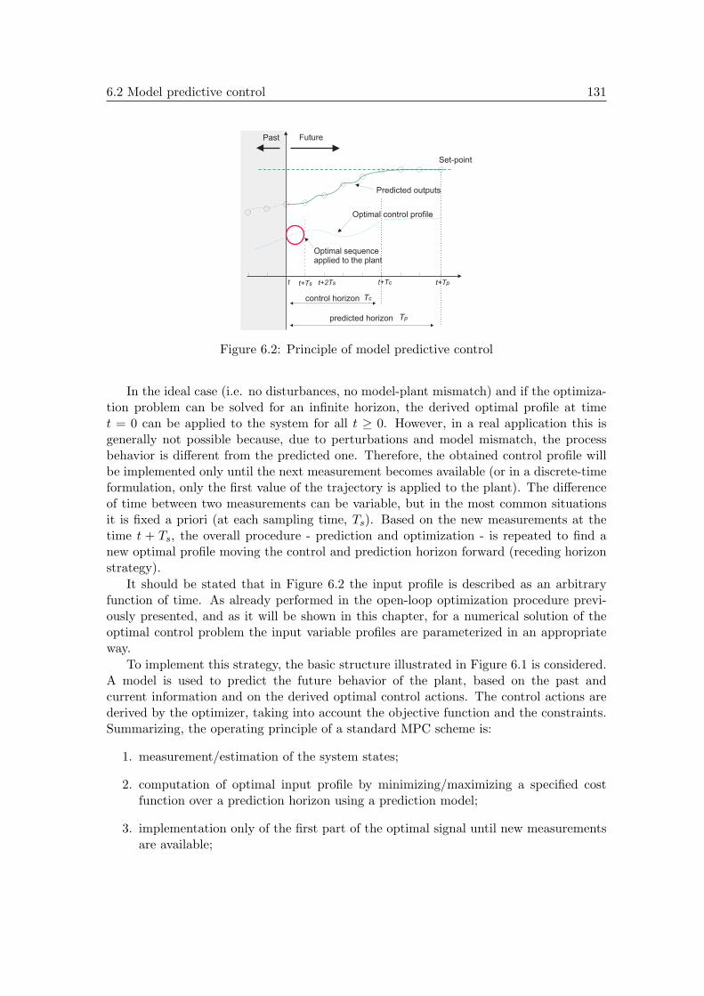
6.2 Model predictive control 131
Past Future
Set-point
Optimal control profile
Optimal sequenceapplied to the plant
control horizon
predicted horizon
t t+Tc t+Tpt+Ts t+2Ts
Predicted outputs
Tc
Tp
Figure 6.2: Principle of model predictive control
In the ideal case (i.e. no disturbances, no model-plant mismatch) and if the optimiza-tion problem can be solved for an infinite horizon, the derived optimal profile at timet = 0 can be applied to the system for all t ≥ 0. However, in a real application this isgenerally not possible because, due to perturbations and model mismatch, the processbehavior is different from the predicted one. Therefore, the obtained control profile willbe implemented only until the next measurement becomes available (or in a discrete-timeformulation, only the first value of the trajectory is applied to the plant). The differenceof time between two measurements can be variable, but in the most common situationsit is fixed a priori (at each sampling time, Ts). Based on the new measurements at thetime t + Ts, the overall procedure - prediction and optimization - is repeated to find anew optimal profile moving the control and prediction horizon forward (receding horizonstrategy).
It should be stated that in Figure 6.2 the input profile is described as an arbitraryfunction of time. As already performed in the open-loop optimization procedure previ-ously presented, and as it will be shown in this chapter, for a numerical solution of theoptimal control problem the input variable profiles are parameterized in an appropriateway.
To implement this strategy, the basic structure illustrated in Figure 6.1 is considered.A model is used to predict the future behavior of the plant, based on the past andcurrent information and on the derived optimal control actions. The control actions arederived by the optimizer, taking into account the objective function and the constraints.Summarizing, the operating principle of a standard MPC scheme is:
1. measurement/estimation of the system states;
2. computation of optimal input profile by minimizing/maximizing a specified costfunction over a prediction horizon using a prediction model;
3. implementation only of the first part of the optimal signal until new measurementsare available;
132 Model predictive approach for start-up procedure
4. go to step (2).
Consequently, the process model plays a key role in the MPC controller. The control per-formance depends on the accuracy of the plant model. In fact, in the application of MPCstrategy, two key issues have to be addressed. The first concern is that a reliable modelable to represent the process dynamics with an accurate output prediction is required. Onthe other hand, MPC requires the repeated on-line solution of an optimal control problembased on the dynamic model of the plant to be controlled and a complex model involvespowerful algorithms to solve efficiently the resulting problem. Thus, the second, whichrepresents one of the main limiting factors of the MPC strategies application, is that ateach sampling time the computational effort needed to solve the optimization problem ishigh and efficient algorithms compatible with real-time implementation are required. Theimplementation becomes more challenging when nonlinear models are used (NMPC).
6.2.2 Solution of the NMPC problem
In the literature different approaches to solve on-line NMPC problems exist, the mostpopular being so-called direct methods briefly presented in the previous chapter [132],[133]. In these approaches, the control, constraints and/or state variables are finitely pa-rameterized, and thus an approximation of the original open-loop optimal control problemis sought. The resulting finite dimensional dynamic optimization problem is then solvedwith standard optimization techniques. Nevertheless, as previously stated, the applicabil-ity of these methods is currently limited for Modelica physical models. Therefore, to solvethe optimal control problem at each sampling time, the open-loop optimization proceduredescribed in the previous chapter has been adapted and used.
6.3 GT load profile optimization. Predictive approach
The predictive method proposed in this section focuses on the determination of the GTload profile. In general, the severity of thermo-mechanical stresses depend on the initialmetal temperatures of the components before start-up, and on the GT loading ratesapplied throughout the start-up process. Consequently, to achieve a minimum start-uptime, the controller must consistently manipulate the fastest instantaneous loading rates,while keeping the stresses under admissible limits. This is specifically the goal of thecontrol strategy described in the following sections. However, the procedure can targetalso the other control variables of the plant.
For the application in a predictive approach, the mathematical formulation of theopen-loop optimal control problem outlined in Chapter 5 has been slightly changed. Inthe sequel, the adopted continuous time formulation and resolution of NMPC for theCCPP start-up problem are presented.

6.3 GT load profile optimization. Predictive approach 133
6.3.1 NMPC problem formulation
Following the notation in Chapter 5, the combined cycle system dynamics can be describedas:
x(t) = f(x(t), z(t), u(t), L(t, q), t, p)
0 = g(x(t), z(t), u(t), L(t, q), t, p)(6.1)
with differential state variables x(t), algebraic state variables z(t) , control variables thatare not concerned by the optimization procedure u(t), control variable to optimize repre-sented by using a finite parameterization L(t, q) (GT load profile) and time-independentparameters p.
Objective function definition
The objective in this approach is defined by means of an integral square error criterion,penalizing the deviation of the control input from its target value (LM ). In fact, with thiscost function, as in the case of ”just-in-time” start-up problem, the computed solution isoptimal in the sense that GT load is increased as fast as possible without violating theimposed constraints. Thus, by increasing the GT load with a maximum allowable loadingrate, a minimum start-up time is assumed to be provided.
In the NMPC problem, at every sampling instant, the input applied to the system isgiven by the solution of the following finite horizon open-loop optimal control problem:
Problem 1.
Find
minq
J(x(t), L(t, q), Tp, Tc)
with
J(x(t), L(t, q), Tp, Tc) =
∫ iTs+Tp
iTs
(L(t, q)− LM )2dt (6.2)
subject to the plant dynamics (6.1) and
c(x(t)) ≤ 0, ∀t ∈ [iTs, iTs + Tp] (6.3)
where i ∈ N is an index used to define the sampling time Ts, Tp and Tc are the output andcontrol prediction horizons. For the approach considered in this section, it is assumed thatthe output prediction horizon is set equal to the control horizon Tp = Tc. The constraint(6.3) represents, in a general form, all the constraints to be imposed on the plant variablesduring the start-up, in particular on the stress level.
The parameter vector q is computed by solving Problem 1, and the receding horizonparadigm is adopted. Thus, only the optimal profile L∗(t, q) computed for t ∈ [iTs, (i +1)Ts] is applied to the system and the overall procedure is repeated at the next samplingperiod Ts.
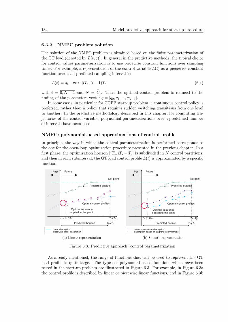
134 Model predictive approach for start-up procedure
6.3.2 NMPC problem solution
The solution of the NMPC problem is obtained based on the finite parameterization ofthe GT load (denoted by L(t, q)). In general in the predictive methods, the typical choicefor control values parameterization is to use piecewise constant functions over samplingtimes. For example, a representation of the control variable L(t) as a piecewise constantfunction over each predicted sampling interval is:
L(t) = qi, ∀t ∈ [iTs, (i+ 1)Ts] (6.4)
with i = 0, N − 1 and N =Tp
Ts. Thus the optimal control problem is reduced to the
finding of the parameters vector q = [q0, q1, ..., qN−1].In some cases, in particular for CCPP start-up problem, a continuous control policy is
preferred, rather than a policy that requires sudden switching transitions from one levelto another. In the predictive methodology described in this chapter, for computing tra-jectories of the control variable, polynomial parameterizations over a predefined numberof intervals have been used.
NMPC: polynomial-based approximations of control profile
In principle, the way in which the control parameterization is performed corresponds tothe one for the open-loop optimization procedure presented in the previous chapter. In afirst phase, the optimization horizon [iTs, iTs + Tp] is subdivided in N control partitions,and then in each subinterval, the GT load control profile L(t) is approximated by a specificfunction.
Past Future
Set-point
Predicted horizon T =Tp c
iT +Ts piTs (i+1)Ts
Optimal sequenceapplied to the plant
Optimal control profiles
Predicted outputs
linear descriptionpiecewise linear description
(a) Linear representation
Past Future
Set-point
Predicted horizon T =Tp c
iT +Ts piTs (i+1)Ts
Optimal sequenceapplied to the plant
Optimal control profiles
smooth descriptionpiecewisedescription based on Lagrange polynomials
Predicted outputs
(b) Smooth representation
Figure 6.3: Predictive approach: control parameterization
As already mentioned, the range of functions that can be used to represent the GTload profile is quite large. The types of polynomial-based functions which have beentested in the start-up problem are illustrated in Figure 6.3. For example, in Figure 6.3athe control profile is described by linear or piecewise linear functions, and in Figure 6.3b
6.3 GT load profile optimization. Predictive approach 135
by functions with a specific degree of smoothness. It should be pointed out that in thepredictive approach for the GT load description, additionally to the case studies presentedin the open-loop procedure, a parameterization based on the Lagrange polynomials hasbeen used in order to increase the control performance. This parameterization is describedbelow.
Lagrange polynomial based parameterization
Considering n+1 points t0, ..., tn ∈ [iTs, iTs+Tp], with n ≥ 1, and the corresponding GTload values at these points L0, ..., Ln, the Lagrange interpolation polynomial of degree nused to describe the GT load profile is formally stated as follows:
Ln(t) =
n∑
j=0
Ljlnj (t) (6.5)
where lnj represent Lagrange basis polynomials defined as:
lnj (t) = 1, n = 1
lnj (t) =
n∏
k=0k 6=j
t− tktj − tk
, n ≥ 2 (6.6)
with 0 ≤ j ≤ n.This type of representation has the advantage that it can be easily implemented com-
pared with that based on quadratic spline functions, providing similar performances (seeSection 6.3.4). It represents an alternative for the use of quadratic splines, but as forthese functions the number of elements in each optimization interval is limited (in thiscase is typically lower than 10). A description of this parameterization with applicationresults can be found in [134].
6.3.3 Implementation of the predictive approach
The MPC controller has been implemented in Matlab, and uses for the resolution ofthe optimization problem the nonlinear solver fmincon. In order to enable and facilitatethe use of the smooth CCPP model for periodic simulations in the MPC algorithm, themodel description has been compiled into an executable code (dymosim.exe) [8]. Thedymosim executable is a stand-alone program which can be directly called from Matlab.This program can use specific files to define its inputs and initial conditions, perform asimulation run, store the results into an output file, etc. For example, when a Dymolamodel is simulated, an input file (dsin.txt) is read that contains all the initial values of thevariables including the states of the system. Therefore, the Dymola files together with theCCPP description (dymosim.exe), have been used to periodically restart the simulationfrom a given point, making it possible to update the current state of the model and toapply the receding horizon paradigm. More details about dymosim executable, Dymolafiles specification and the way in which a Modelica model can be executed are given inAppendix G.

136 Model predictive approach for start-up procedure
In general, the derivation of predictive control law is based on the knowledge of thecomplete state of the system. The feature that the model representation can use files todefine conditions of experiment (variables, parameters) and to provide complete informa-tion about the state variables of the system has been exploited in the implementation ofthe MPC controller. Thus, at each sampling time the determination of the current stateand the initialization of the model in the specified state have been carried out using theresults file generated by simulation.
The entire procedure has been coded in Matlab and included in the control algorithm.The adopted NMPC control loop with the physical plant represented by the Modelica/Dy-mola system is outlined in Figure 6.4a.
optimization
model prediction
controlactions
objective,constraints
Matlab/Dymolaprocedure
Modelica/Dymolasystem
controlinputs
u
outputfile
inputfile
currentstate
-dymosim.exe
MPC controller
(a) Adopted control loop
optimization
model prediction
controlactions
objective,constraints
Observer
P lantcontrolinputs
u
y
x
MPC controller
(b) Classical control loop
Figure 6.4: NMPC control loop
Therefore, the elaboration of the control law has been conducted assuming that thecomplete states of the system are known, which is not generally true in the case of areal plant. In a real control environment, the measurement of the state variables of thesystem is often not available, either very expensive or even impossible. The most popularsolution to this problem is the use of an observer that reconstructs the state variablesusing a dynamic model of the physical system, the inputs and the available measurablephysical outputs of the system (see Figure 6.4b). However, the design of such an observeris beyond the scope of this work.
6.3.4 Simulation results
In the preceding paragraphs, the predictive approach of the GT load profile for the CCPPstart-up problem has been presented.
The purpose of this section is to compare the predictive algorithm results with the onesobtained by applying the open-loop optimization procedure implemented in Chapter 5.To do this, the control algorithm has been applied to last stage of the start-up sequence,considering the same initial conditions as in Section 5.3. Also, the admissible limits ofthe constraints that act on the plant variables are maintained the same.
To illustrate the advantages and the limitations of the predictive approach, severalscenarios have been studied, varying the MPC control parameters and the type of pa-
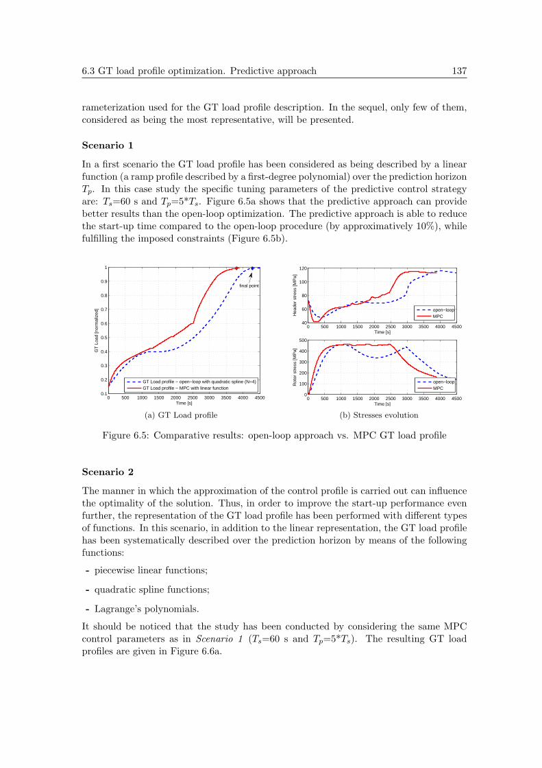
6.3 GT load profile optimization. Predictive approach 137
rameterization used for the GT load profile description. In the sequel, only few of them,considered as being the most representative, will be presented.
Scenario 1
In a first scenario the GT load profile has been considered as being described by a linearfunction (a ramp profile described by a first-degree polynomial) over the prediction horizonTp. In this case study the specific tuning parameters of the predictive control strategyare: Ts=60 s and Tp=5*Ts. Figure 6.5a shows that the predictive approach can providebetter results than the open-loop optimization. The predictive approach is able to reducethe start-up time compared to the open-loop procedure (by approximatively 10%), whilefulfilling the imposed constraints (Figure 6.5b).
0 500 1000 1500 2000 2500 3000 3500 4000 45000.1
0.2
0.3
0.4
0.5
0.6
0.7
0.8
0.9
1
Time [s]
GT
Loa
d [n
orm
aliz
ed]
GT Load profile − open−loop with quadratic spline (N=4) GT Load profile − MPC with linear function
final point
(a) GT Load profile
0 500 1000 1500 2000 2500 3000 3500 4000 450040
60
80
100
120
Time [s]
Hea
der
stre
ss [M
Pa]
0 500 1000 1500 2000 2500 3000 3500 4000 45000
100
200
300
400
500
Time [s]
Rot
or s
tres
s [M
Pa]
open−loopMPC
open−loopMPC
(b) Stresses evolution
Figure 6.5: Comparative results: open-loop approach vs. MPC GT load profile
Scenario 2
The manner in which the approximation of the control profile is carried out can influencethe optimality of the solution. Thus, in order to improve the start-up performance evenfurther, the representation of the GT load profile has been performed with different typesof functions. In this scenario, in addition to the linear representation, the GT load profilehas been systematically described over the prediction horizon by means of the followingfunctions:
- piecewise linear functions;
- quadratic spline functions;
- Lagrange’s polynomials.
It should be noticed that the study has been conducted by considering the same MPCcontrol parameters as in Scenario 1 (Ts=60 s and Tp=5*Ts). The resulting GT loadprofiles are given in Figure 6.6a.
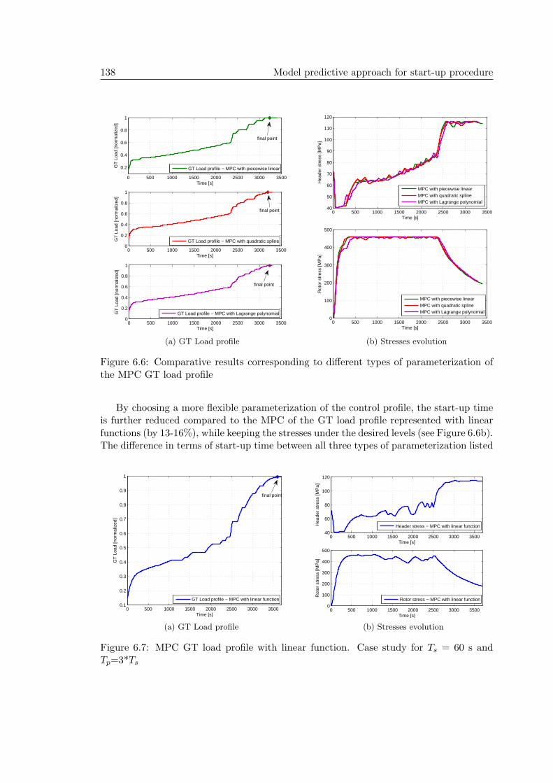
138 Model predictive approach for start-up procedure
0 500 1000 1500 2000 2500 3000 3500
0.2
0.4
0.6
0.8
1
Time [s]
GT
Loa
d [n
orm
aliz
ed]
0 500 1000 1500 2000 2500 3000 35000
0.2
0.4
0.6
0.8
1
Time [s]
GT
Loa
d [n
orm
aliz
ed]
0 500 1000 1500 2000 2500 3000 35000
0.2
0.4
0.6
0.8
1
Time [s]
GT
Loa
d [n
orm
aliz
ed]
GT Load profile − MPC with piecewise linear
GT Load profile − MPC with quadratic spline
GT Load profile − MPC with Lagrange polynomial
final point
final point
final point
(a) GT Load profile
0 500 1000 1500 2000 2500 3000 350040
50
60
70
80
90
100
110
120
Time [s]
Hea
der
stre
ss [M
Pa]
0 500 1000 1500 2000 2500 3000 35000
100
200
300
400
500
Time [s]
Rot
or s
tres
s [M
Pa]
MPC with piecewise linearMPC with quadratic splineMPC with Lagrange polynomial
MPC with piecewise linearMPC with quadratic splineMPC with Lagrange polynomial
(b) Stresses evolution
Figure 6.6: Comparative results corresponding to different types of parameterization ofthe MPC GT load profile
By choosing a more flexible parameterization of the control profile, the start-up timeis further reduced compared to the MPC of the GT load profile represented with linearfunctions (by 13-16%), while keeping the stresses under the desired levels (see Figure 6.6b).The difference in terms of start-up time between all three types of parameterization listed
0 500 1000 1500 2000 2500 3000 35000.1
0.2
0.3
0.4
0.5
0.6
0.7
0.8
0.9
1
Time [s]
GT
Loa
d [n
orm
aliz
ed]
GT Load profile − MPC with linear function
final point
(a) GT Load profile
0 500 1000 1500 2000 2500 3000 350040
60
80
100
120
Time [s]
Hea
der
stre
ss [M
Pa]
0 500 1000 1500 2000 2500 3000 35000
100
200
300
400
500
Time [s]
Rot
or s
tres
s [M
Pa]
Header stress − MPC with linear function
Rotor stress − MPC with linear function
(b) Stresses evolution
Figure 6.7: MPC GT load profile with linear function. Case study for Ts = 60 s andTp=3*Ts

6.3 GT load profile optimization. Predictive approach 139
above is really quite low (equal to the sampling time of 60 s, see also Table 6.1). In thiscase the gain brought by a more flexible profile (e.g., quadratic spline) is less importantthan for the open-loop approach. Also, the use of such functions for profile descriptioninvolves a computation time well above the limits for a real-time implementation.
In the considered predictive approach the solution that ensures the best trade-offbetween start-up performance and computation time is carried out by approximating theGT load profile by means of a linear function over the prediction horizon, together withan appropriate tuning of the control parameters (Figure 6.7a). It enables to obtain a gainin start-up time comparable to that provided by a more accurate description of the GTload profile (a lower gain up to 12%), without exceeding the stress limits (Figure 6.7b).
In general, simplified representations are desirable from the point of view of the com-putational effort. This fact can be observed from the computation time needed to solvethe overall optimization process for each type of parameterization (see Table 6.1), wherefor the MPC with a linear representation of the GT load profile the computation time isconsiderably lower than in other cases.
Scenario 3
By adopting the predictive control strategy, the potential delay between changes in theloading rate and their effects on the process variables, in particular on the header andsteam turbine stresses, can be anticipated. An important role in this strategy is playedby the prediction horizon.
In general in industrial application of NMPC, in order to achieve specific controlperformance a long prediction horizon is required. Moreover, the nominal stability ofthe closed-loop is relied on the selection of long horizons. On the other hand, from acomputational point of view short prediction horizons are preferable [135].
In this scenario the length of the prediction horizon has been varied to show how itcan influence the start-up performance. Also, for obtaining high controller performances,different values of the sampling time has been chosen. The obtained results are presentedin Figure 6.8.
The selection of sampling time Ts and prediction horizon Tp is important in the imple-mentation of the MPC start-up controller. As shown in Figure 6.8 the trend for obtainingthe highest start-up performances is to select a short prediction horizon. In fact, theprediction horizon Tp, which together with the control profile approximation directly in-fluence the computational effort to solve Problem 1, is limited by the efficiency of theoptimization algorithm. Also, the manner in which the sampling is chosen can influencethe optimality of the solution. The fact that at each control step the approximation of theoptimal solution is not performed with accuracy requires a frequent computation of thecontrol profile, involving a short sampling time. In turn, a short sampling time involvesan increased number of optimization problems solved during the start-up, resulting in ahigher overall computation time (6.8b). It should be pointed out that the minimum valueof the look-ahead time has been selected to be longer than the dominant time constantof the system, a necessary condition to avoid issues linked to an insufficient predictiontime. A complete comparison in terms of start-up performances and computation timebetween different types of profile-functions used for the GT load description and control
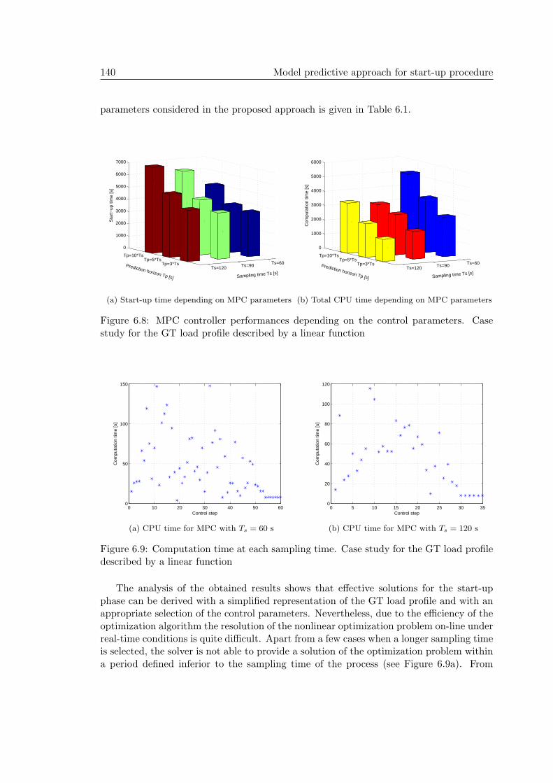
140 Model predictive approach for start-up procedure
parameters considered in the proposed approach is given in Table 6.1.
Ts=60Ts=90Ts=120Tp=3*Ts
Tp=5*TsTp=10*Ts
0
1000
2000
3000
4000
5000
6000
7000
Sampling time Ts [s]
Prediction horizon Tp [s]
Sta
rt−
up ti
me
[s]
(a) Start-up time depending on MPC parameters
Ts=60Ts=90Ts=120Tp=3*Ts
Tp=5*TsTp=10*Ts
0
1000
2000
3000
4000
5000
6000
Sampling time Ts [s]
Prediction horizon Tp [s]
Com
puta
tion
time
[s]
(b) Total CPU time depending on MPC parameters
Figure 6.8: MPC controller performances depending on the control parameters. Casestudy for the GT load profile described by a linear function
0 10 20 30 40 50 600
50
100
150
Control step
Com
puta
tion
time
[s]
(a) CPU time for MPC with Ts = 60 s
0 5 10 15 20 25 30 350
20
40
60
80
100
120
Control step
Com
puta
tion
time
[s]
(b) CPU time for MPC with Ts = 120 s
Figure 6.9: Computation time at each sampling time. Case study for the GT load profiledescribed by a linear function
The analysis of the obtained results shows that effective solutions for the start-upphase can be derived with a simplified representation of the GT load profile and with anappropriate selection of the control parameters. Nevertheless, due to the efficiency of theoptimization algorithm the resolution of the nonlinear optimization problem on-line underreal-time conditions is quite difficult. Apart from a few cases when a longer sampling timeis selected, the solver is not able to provide a solution of the optimization problem withina period defined inferior to the sampling time of the process (see Figure 6.9a). From

6.3 GT load profile optimization. Predictive approach 141
the computation time point of view, more suitable solutions can be given when a largesampling time is chosen, but in this case the solution is sub-optimal in terms of start-uptime (Figure 6.9b).
GT load profile optimization
Function Control Start-up Time Fuel CPUparameters time [s] gain [%] saving [%] time1[s]
standard seq. - - 6038 - -
open-loop- 4278 - - -
quadratic spline
linear
Ts = 60 s Tp = 3 ∗ Ts 3600≈16* ≈14*
2884≈40** ≈43**
Ts = 60 s Tp = 5 ∗ Ts 3840≈10* ≈5*
3776≈36** ≈38**
Ts = 90 s Tp = 3 ∗ Ts 3780≈11* ≈8*
1942≈37** ≈39**
Ts = 120 s Tp = 3 ∗ Ts 4200≈2* -*
1563≈30** ≈38**
piecewiseTs = 60 s Tp = 5 ∗ Ts 3240
≈25* ≈23*12851
linear ≈46** ≈49**
quadraticTs = 60 s Tp = 5 ∗ Ts 3180
≈26* ≈25*14831
spline ≈47** ≈49**
Lagrange’sTs = 60 s Tp = 5 ∗ Ts 3240
≈25* ≈23*6218
polynomial ≈46** ≈48**
1 overall CPU time computed for optimization process* related to the open-loop procedure** related to the standard procedure with a constant GT Load ramp 2 MW/min
Table 6.1: Comparative results Model Predictive Control of the GT load profile
Summarizing, the GT load profiles issued from the MPC strategy are adapted for thecurrent plant state and are generated with a specific prediction capability. Therefore,with an accurate estimation of future evolution of the plant behavior, in particular of thestresses (rotor and header), the MPC load can be more aggressive, without exceeding theadmissible limits. As a result, the new controller has been able to complete the start-upphase by about 18 minutes faster than the open-loop approach and by 47 minutes fasterthan a standard start-up procedure. Despite this, due to the computational burden, atthis stage, an effective solution in terms of start-up time, which at the same time isimplementable under real-time conditions can not be provided. A solution in this sensewill be given in the next section.

142 Model predictive approach for start-up procedure
6.4 Hierarchical model predictive control approach
Hierarchical control has received a significant attention during the last decades [136]. Theinterest is mainly motivated by the fact that an important number of systems can be bet-ter controlled with hierarchical structures than with classic control methodologies. Amongthem, we can mention the design of controllers for multi-time scale systems characterizedby clearly separable slow and fast dynamics (based on e.g., cascade structures), hierar-chical structures used to coordinate a number of local controllers (e.g., for the controlof a power plant [130]), the design of controllers for plants characterized by an inherenthierarchical structure. A complete discussion can be found in the reports of the HD-MPCproject1 (see for example [137], [138]) and the many references therein.
Also, given the difficulty to control large-scale systems with centralized control struc-ture due to the required computational complexity, the application of MPC approachin hierarchical and distributed control architectures shows a high potential. In manysituations, sharing information between local regulator designed with MPC and/or be-tween different control layers about the future control actions and the corresponding statetrajectories involves performances comparable to those ideally provided by a centralizedcontrol structure.
In the case of the CCPP start-up problem, the application of a hierarchical controlstructure is motivated by two aspects. The first aspect is that the combined cycle powerplants are complex systems composed by many interacting subsystems that are generallycontrolled by means of a hierarchical structure, where the upper layer coordinates thelocal controllers. The second aspect is that the computational burden of the optimizationproblem to be solved at each control step is high, and the proposed MPC solution canbe considered inconsistent for a real-time implementation (which was the case in pre-vious section). Therefore, in order to obtain more real implementable results, the MPCframework has been redesigned and extended to a hierarchical predictive control structure(H-MPC) in which two controllers tackle different objectives.
6.4.1 Hierarchical structure
The proposed hierarchical structure includes two layers with different time scales: a high(HL) and a low layer (LL). At the high level a minimum time optimal control problemis solved over a long time period. The solution of this problem is used to update theGT load set-point for the low level, where a constrained tracking optimization problemis solved over a shorter period. It should be noticed that in this case the MPC problemsfor each layer are formulated based on the same Modelica model and not on models withdifferent dynamic behaviors as in the most common approaches proposed in the literature[139].
The objective of the hierarchical approach is to create a control structure with moresuitable optimization problems in terms of computation time. The underlying idea is tohave at the high level an optimization problem that derives suboptimal profiles of the GTload, enabling to be quickly solved. Then, at the low level the information provided by
1Hierarchical and Distributed Model Predictive Control of Large-Scale Systems, http://www.ict-hd-mpc.eu/

6.4 Hierarchical model predictive control approach 143
the high level is used for obtaining a more tractable optimization problem, which refinesthe GT load profiles in order to reach an optimal solution.
6.4.2 H-MPC problem formulation
The problem is formulated for the high and low layers, where the control variable ofinterest is the load of the GT.
Consider that the CCPP model can be given in two dynamic explicit forms, corre-sponding to each level:
• high level:
x(t) = f(x(t), z(t), u(t), Lh(t), t, p)
0 = g(x(t), z(t), u(t), Lh(t), t, p)(6.7)
• low level:
x(t) = f(x(t), z(t), u(t), Ll(t), t, p)
0 = g(x(t), z(t), u(t), Ll(t), t, p)(6.8)
where Lh(t) is the GT load control variable associated with the high level, while Ll(t) isthe refined GT load control variable corresponding to the low level.
Assumption 6.4.1. The GT load profile for each level is described by a parameterizedfunction, Lh(t, qh), Ll(t, ql), with qh and ql the parameter vectors that are derived throughoptimization.
In the H-MPC approach, for each layer a different sampling time is defined. In thesequel, Th and Tl represent the sampling times for high level and low level respectively.
Remark 6.4.1. For simplicity, a relationship between Th and Tl is fixed, by introducinga time ratio, k ∈ N so that Th = kTl, with k ≥ 1.
Remark 6.4.2. At each level different horizons are associated; a long horizon correspondsto the high level while for the low level a short prediction horizon is considered.
6.4.2.1 Optimization problem for the high level
The goal of the optimization problem is to find the GT load profile that minimizes thestart-up time, while fulfilling constraints on the process variables. The problem corre-sponds to the open-loop optimization presented in the previous chapter.
At each HL sample time iTh, the GT load control profile, described by Lh(t, qh), iscomputed as a result of the following minimum time problem:
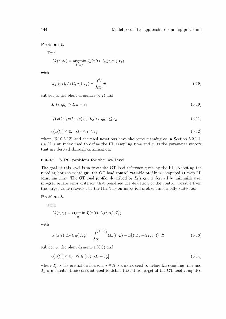
144 Model predictive approach for start-up procedure
Problem 2.
Find
L∗h(t, qh) = argmin
qh,tf
Jh(x(t), Lh(t, qh), tf )
with
Jh(x(t), Lh(t, qh), tf ) =
∫ tf
iTh
dt (6.9)
subject to the plant dynamics (6.7) and
L(tf , qh) ≥ LM − ǫ1 (6.10)
|f(x(tf ), u(tf ), z(tf ), Lh(tf , qh)| ≤ ǫ2 (6.11)
c(x(t)) ≤ 0, iTh ≤ t ≤ tf (6.12)
where (6.10-6.12) and the used notations have the same meaning as in Section 5.2.1.1,i ∈ N is an index used to define the HL sampling time and qh is the parameter vectorsthat are derived through optimization.
6.4.2.2 MPC problem for the low level
The goal at this level is to track the GT load reference given by the HL. Adopting thereceding horizon paradigm, the GT load control variable profile is computed at each LLsampling time. The GT load profile, described by Ll(t, ql), is derived by minimizing anintegral square error criterion that penalizes the deviation of the control variable fromthe target value provided by the HL. The optimization problem is formally stated as:
Problem 3.
Find
L∗l (t, ql) = argmin
ql
Jl(x(t), Ll(t, ql), Tp)
with
Jl(x(t), Ll(t, ql), Tp) =
∫ jTl+Tp
jTl
(Ll(t, ql)− L∗h(iTh + Tk, qh))
2dt (6.13)
subject to the plant dynamics (6.8) and
c(x(t)) ≤ 0, ∀t ∈ [jTl, jTl + Tp] (6.14)
where Tp is the prediction horizon, j ∈ N is a index used to define LL sampling time andTk is a tunable time constant used to define the future target of the GT load computed

6.4 Hierarchical model predictive control approach 145
by the HL. The constraint (6.14), as in other optimization problems, includes all theconstraints imposed on the plant variables during start-up phase.
Then, according to the receding horizon paradigm, only the optimal profile computedfor t ∈ [jTl, (j + 1)Tl] is applied to the system and the overall procedure is repeated at anew sampling period.
The optimization problem at the low level (Problem 3) aims the same objective as the1-level MPC controller (Problem 2), namely the minimization of the squared deviationsfrom the target point. The difference is made by the target point that in the hierarchicalstructure is defined at each HL sampling time by the upper optimization problem, whilein the 1-level MPC it corresponds to the full load.
Remark 6.4.3. The reference from HL is considered as a constant along the interval[jTl, jTl + Tp] to facilitate the communication between layers.
6.4.3 H-MPC multilevel algorithm
The hierarchical approach presented above has been integrated in an MPC multilevel al-gorithm. The algorithm with the principle adopted for the communication of informationbetween the layers can be stated as:
Basic algorithm:
HL: - at the time instant iTh:
• the optimization problem corresponding to the high level (Problem 2) is solved
• the solution determined at the predefined instant Tk, L∗h(iTh+Tk, qh), is sent
to the low level
- the procedure is repeated after each time instant Th (i := i + 1) with the newstates provided by the plant
LL: - at every instant jTl:
• the corresponding MPC problem for the low level (Problem 3) is solved byusing the reference signal provided by high level optimization
- according to the receding horizon paradigm:
• only the optimal profile computed for t ∈ [jTl, (j + 1)Tl] is applied to thesystem
• the overall procedure is repeated at a new sampling period Tl (j := j + 1),with the current plant states
The adopted structure of the hierarchical controller is illustrated in Figure 6.10a. Also,Figure 6.10b shows the temporal diagram of the approach.
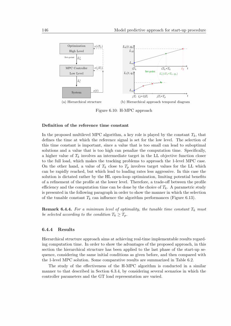
146 Model predictive approach for start-up procedure
Optimization
High Level
MPC Controller
Low Level
Systemx(t)
x(jTl)
x(iTh)
L∗
hSet-point
L∗
l
(a) Hierarchical structure
jTl
iTh
(j+1)Tl jTl+Tp t
ttfiTh+Tk
Ll(t, ql)
Lh(t, qh)
Lm
Lm
LM
Set-pointL∗
h(iTh+Tk, qh)
(b) Hierarchical approach temporal diagram
Figure 6.10: H-MPC approach
Definition of the reference time constant
In the proposed multilevel MPC algorithm, a key role is played by the constant Tk, thatdefines the time at which the reference signal is set for the low level. The selection ofthis time constant is important, since a value that is too small can lead to suboptimalsolutions and a value that is too high can penalize the computation time. Specifically,a higher value of Tk involves an intermediate target in the LL objective function closerto the full load, which makes the tracking problems to approach the 1-level MPC case.On the other hand, a value of Tk close to Tp involves target values for the LL whichcan be rapidly reached, but which lead to loading rates less aggressive. In this case thesolution is dictated rather by the HL open-loop optimization, limiting potential benefitsof a refinement of the profile at the lower level. Therefore, a trade-off between the profileefficiency and the computation time can be done by the choice of Tk. A parametric studyis presented in the following paragraph in order to show the manner in which the selectionof the tunable constant Tk can influence the algorithm performances (Figure 6.13).
Remark 6.4.4. For a minimum level of optimality, the tunable time constant Tk mustbe selected according to the condition Tk ≥ Tp.
6.4.4 Results
Hierarchical structure approach aims at achieving real-time implementable results regard-ing computation time. In order to show the advantages of the proposed approach, in thissection the hierarchical structure has been applied to the last phase of the start-up se-quence, considering the same initial conditions as given before, and then compared withthe 1-level MPC solution. Some comparative results are summarized in Table 6.2.
The study of the effectiveness of the H-MPC algorithm is conducted in a similarmanner to that described in Section 6.3.4, by considering several scenarios in which thecontroller parameters and the GT load representation are varied.

6.4 Hierarchical model predictive control approach 147
GT load profile optimization
Approach Control Start-up Time Fuel CPU time [s]parameters time [s] gain [%] saving [%] total mean
standard - - 6038 - - - -
open-loop - 4278 - - - -
MPCTs = 60 s Tp = 3 ∗ Ts 3600 ≈40* ≈43* 2884 48
S1
H-MPC Tl = 60 s Tp = 3 ∗ Tl3600 ≈40* ≈43* 1425
10.5HL
S1 Th = 2 ∗ Tl Tk = 5 ∗ Tp 18.2LL
MPCTs = 60 s Tp = 3 ∗ Ts 3240 ≈46* ≈48* 6218 115.1
S3
H-MPC Tl = 60 s Tp = 5 ∗ Tl3240 ≈46* ≈48* 2949
9.6HL
S3 Th = 3 ∗ Tl Tk = 2 ∗ Tp 51.2LL
* related to the standard procedureHL High Level mean computation timeLL Low Level mean computation timeS1 Scenario 1: MPC with GT load profile described by linear functionsS3 Scenario 3: MPC with GT load profile described by Lagrange polynomials
Table 6.2: Results comparison MPC vs. H-MPC
Scenario 1
In this scenario, a linear representation of the GT load profile has been considered for eachMPC controller. Also, to compare the performance of the H-MPC algorithm with respectto the 1-level MPC solution, the parameters of the 1-level MPC controller correspond tothose of the LL controller of H-MPC, namely:
• MPC: Ts = 60 s, Tp = 3 ∗ Ts;
• H-MPC:
– LL: Tl = Ts, Tp = 3 ∗ Tl;
– HL: Th = 2 ∗ Tl, Tk = 5 ∗ Tp.
The experimental results in terms of computation time at each control step are given inFigure 6.11. Visibly, the main advantage of the application of the hierarchical structure isthat it enables the reduction of the computation time. In the case of the H-MPC algorithmapplication, the time required to solve the optimization problem at each control step islower than the sampling period (see Figure 6.11). Furthermore, the hierarchical approachbased on a consistent estimation of the future behavior of the plant, together with aperiodic computation of the GT load profile, derives an optimal profile that leads to afast start-up phase (see Figure 6.12a), while maintaining the lifetime consumption of themost stressed components under control (see Figure 6.12b). As can be seen from Table6.2, the hierarchical approach leads to start-up performances comparable to those of the

148 Model predictive approach for start-up procedure
one level MPC solution, but with a significant reduction of the total computation time(over 50%).
0 10 20 30 40 50 600
60
100
150
Control step
Com
puta
tion
time
[s]
MPCH−MPC
Figure 6.11: Computation time at each sampling time MPC vs. H-MPC. Case study for:{Ts = 60 s, Tp = 3 ∗Ts}MPC , {Tl = Ts, Tp = 3 ∗Tl, Th = 2 ∗Tl, Tk = 5 ∗Tp}H−MPC , withGT load profile described by a linear function
0 500 1000 1500 2000 2500 3000 35000.1
0.2
0.3
0.4
0.5
0.6
0.7
0.8
0.9
1
Time [s]
GT
Loa
d [n
orm
aliz
ed]
MPCH−MPC
final point
(a) GT Load profile
0 500 1000 1500 2000 2500 3000 35000
200
400
600
Time [s]
Rot
or S
tres
s [M
Pa]
0 500 1000 1500 2000 2500 3000 350040
60
80
100
120
Time [s]
Hea
dear
Str
ess
[MP
a]
MPCH−MPC
MPCH−MPC
(b) Header stress and Rotor stress results
Figure 6.12: Results comparison MPC vs. H-MPC. Case study for: {Ts = 60 s, Tp =3∗Ts}MPC , {Tl = Ts, Tp = 3∗Tl, Th = 2∗Tl, Tk = 5∗Tp}H−MPC , with GT load describedby a ramp profile
Scenario 2
The key of the hierarchical algorithm is represented by the use of intermediate load-pointsto define the target in the low level objective function. The full load target in the LLcontroller, initially considered in the 1-level MPC, has been replaced with intermediate

6.4 Hierarchical model predictive control approach 149
points generated by the HL in order to provide to the solver a more suitable trackingproblem.
In the H-MPC algorithm the definition of the LL targets-load is updated at eachTk period. The selection of the constant Tk at which the reference signal is set to theLL influences the quality of the solution. In order to show how the tunable algorithmparameter Tk can influence the solution of the H-MPC problem, the results of a parametricstudy are presented in Figure 6.13. The case study has been performed for a descriptionof the GT load profile with a linear function and using the following parameters of theH-MPC controller: Tl = 60 s, Th = 2 ∗ Tl, Tp = 3 ∗ Tl.
Tp 3*Tp 5*Tp 7*Tp 9*Tp600
700
800
900
1000
1100
1200
1300
1400
1500
1600
1700
Com
puta
tion
time
[s]
Tk
(a) Influence of Tk on the overall computation time
Tp 3*Tp 5*Tp 7*Tp 9*Tp0
5
10
15
20
25
Sta
rt−
up ti
me
impr
ovem
ent [
%]
Tk
(b) Influence of Tk on the profile optimality
Figure 6.13: Influence of the parameter Tk on the optimization performances. Comparisonstart-up time related to the case Tk=Tp
According to the simulation results, it is apparent that a value of Tk close to the LLprediction horizon leads to profiles which can be quickly derived, but less effective in termsof start-up time; on the other hand, if a higher value is chosen, the corresponding targetstend to full load, resulting in optimal profiles determined with inappropriate computationtimes, but close to those provided by the 1-level MPC solution. In general, a compromisestart-up time/computation time must be done in order to obtain real-time implementableresults. In fact, the proposed approach offers the possibility to make a trade-off betweenstart-up performance and computation time, by selecting the constant that defines thetime at which the set-point is set for the low level.
Scenario 3
The performances of the H-MPC algorithm, as for other proposed solutions, depend onthe accuracy with which the GT load profile is approximated. In the third scenario, theefficiency of the hierarchical algorithm has been tested for more flexible representationsof the GT load profile at the low level. The results presented in Figure 6.14a have beenobtained by considering the GT load profile at the LL described by Lagrange polynomials.At the HL, the same type of representation as in the previous cases, based on a linear
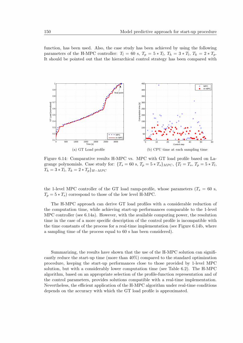
150 Model predictive approach for start-up procedure
function, has been used. Also, the case study has been achieved by using the followingparameters of the H-MPC controller: Tl = 60 s, Tp = 5 ∗ Tl, Th = 3 ∗ Tl, Tk = 2 ∗ Tp.It should be pointed out that the hierarchical control strategy has been compared with
0 500 1000 1500 2000 2500 30000.1
0.2
0.3
0.4
0.5
0.6
0.7
0.8
0.9
1
Time [s]
GT
Loa
d [n
orm
aliz
ed]
MPC H−MPC
final point
(a) GT Load profile
0 10 20 30 40 50 600
50
100
150
200
250
300
350
400
450
Com
puta
tion
time
[s]
Control step
MPCH−MPC
(b) CPU time at each sampling time
Figure 6.14: Comparative results H-MPC vs. MPC with GT load profile based on La-grange polynomials. Case study for: {Ts = 60 s, Tp = 5 ∗ Ts}MPC , {Tl = Ts, Tp = 5 ∗ Tl,Th = 3 ∗ Tl, Tk = 2 ∗ Tp}H−MPC
the 1-level MPC controller of the GT load ramp-profile, whose parameters (Ts = 60 s,Tp = 5 ∗ Ts) correspond to those of the low level H-MPC.
The H-MPC approach can derive GT load profiles with a considerable reduction ofthe computation time, while achieving start-up performances comparable to the 1-levelMPC controller (see 6.14a). However, with the available computing power, the resolutiontime in the case of a more specific description of the control profile is incompatible withthe time constants of the process for a real-time implementation (see Figure 6.14b, wherea sampling time of the process equal to 60 s has been considered).
Summarizing, the results have shown that the use of the H-MPC solution can signifi-cantly reduce the start-up time (more than 40%) compared to the standard optimizationprocedure, keeping the start-up performances close to those provided by 1-level MPCsolution, but with a considerably lower computation time (see Table 6.2). The H-MPCalgorithm, based on an appropriate selection of the profile-function representation and ofthe control parameters, provides solutions compatible with a real-time implementation.Nevertheless, the efficient application of the H-MPC algorithm under real-time conditionsdepends on the accuracy with which the GT load profile is approximated.
6.5 Conclusion 151
6.5 Conclusion
In this final chapter, a Nonlinear Model-based Predictive Controller (NMPC) for CCPPstart-up problem has been proposed. The optimization problem has been formulated inorder to minimize the start-up time subject to the plant dynamics represented by thesmooth Modelica model of the plant and to constraints on the main plant variables. Theoptimization is focused on the GT load profile. Based on the finite parameterization ofthe manipulated variable profile, the same technique as in Chapter 5 has been used forthe resolution of the optimization problem. Different types of profile functions have beentested to achieve efficient solutions.
The predictive approach is a promising control technology for the CCPP start-up.Using a periodic computation of the GT load profile and based on an accurate predictionof the future behavior of the plant, the proposed approach provides high start-up perfor-mances (time, fuel consumption), being able to significantly improve the transient timeas compared to the standard start-up procedure, and even than the open-loop procedurepreviously presented.
The optimal GT load profiles derived from the MPC controller are computed witha specific predictability and adapted to the current process state, resulting in a moreaggressive GT loading rate, without exceeding the stress limits.
However, due to the computational effort to solve the optimization problem at eachcontrol step, the indicated MPC solution has been considered inconsistent for a real-timeimplementation, providing an insufficiently low computation time. A solution in orderto obtain real-time implementable results has been proposed in the second part of thischapter. The suggested solution has been to use a hierarchical predictive control structure(H-MPC) with two levels, in which each controller tackles a different objective. Thehierarchical algorithm has a certain degree of flexibility (start-up efficiency/computationtime) regarding the determination of the optimal solution.
The results emphasize the fact that the use of the H-MPC solution reduces significantlythe start-up time compared with the standard start-up procedure and even with open-loop optimization procedure, keeping the start-up performances close to those providedby 1-level MPC solution, but, the most important aspect, with a lower computation time.
This chapter completes the proposed solutions for the improvement of the CCPP start-up throughout the dissertation. In the next chapter, a synthesis with general conclusionsregarding the presented study is outlined and some perspectives with suggestions for afuture work are provided.

CHAPTER 7
Conclusions and perspectives
The content of this thesis is dedicated to the development of new strategies for the im-provement of the combined cycle power plant start-up efficiency. The proposed strategiesare based on the first-principle model of process using dynamic optimization techniquesfor achieving the intended purposes. The presented chapters include systematically themain phases to develop and implement a model-based approach, detailing every aspectin part: physical modeling, optimization and control. In general, the results are specificfor the CCPP start-up, but many parts can be generalized to other applications of opti-mization and control design. The posed optimal start-up problem has been analyzed andformalized, before explaining the proposed solutions, while emphasizing the contributionsbrought. Each adopted solution has been tested and validated by simulation. In thisfinal chapter, the main results are summarized, and some future research directions arediscussed.
7.1 Synthesis of the work
In the process industry, the safety and the operational availability represents imperativerequirements. Thus, conventional strategies are generally used for the start-up of com-bined cycle power plants. Nevertheless, the traditional techniques are quite conservative,using a series of limitations on the control variable which leads to suboptimal solutions(i.e. a relatively long start-up time, high operating costs, etc.). These limitations areintended to preserve the lifetime consumption of the plant components under control.Due to increasingly stringent economical and environmental specifications, new and ef-ficient management strategies are required for the start-up phase, which ensure the safeoperation of the plant, while keeping the lifetime consumption of the components underspecific levels.
The dynamic optimization for optimal control of the system represents an importantsolution to deal with the improvement of the start-up efficiency. Based on a dynamic
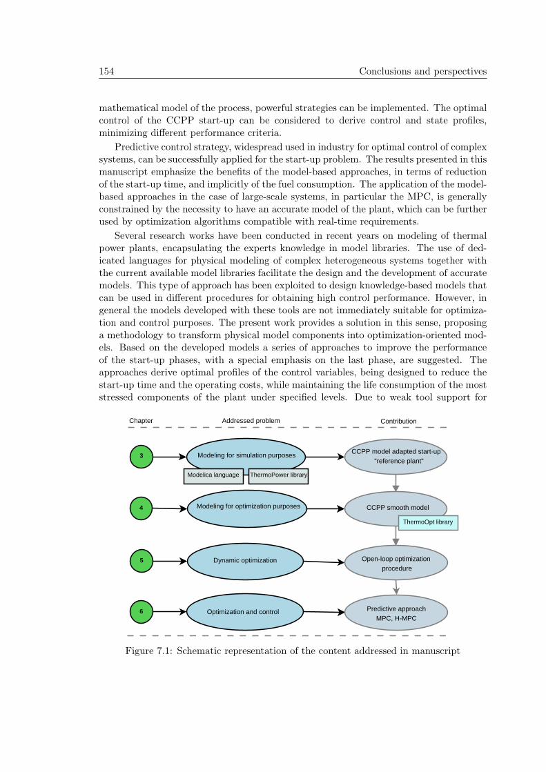
154 Conclusions and perspectives
mathematical model of the process, powerful strategies can be implemented. The optimalcontrol of the CCPP start-up can be considered to derive control and state profiles,minimizing different performance criteria.
Predictive control strategy, widespread used in industry for optimal control of complexsystems, can be successfully applied for the start-up problem. The results presented in thismanuscript emphasize the benefits of the model-based approaches, in terms of reductionof the start-up time, and implicitly of the fuel consumption. The application of the model-based approaches in the case of large-scale systems, in particular the MPC, is generallyconstrained by the necessity to have an accurate model of the plant, which can be furtherused by optimization algorithms compatible with real-time requirements.
Several research works have been conducted in recent years on modeling of thermalpower plants, encapsulating the experts knowledge in model libraries. The use of ded-icated languages for physical modeling of complex heterogeneous systems together withthe current available model libraries facilitate the design and the development of accuratemodels. This type of approach has been exploited to design knowledge-based models thatcan be used in different procedures for obtaining high control performance. However, ingeneral the models developed with these tools are not immediately suitable for optimiza-tion and control purposes. The present work provides a solution in this sense, proposinga methodology to transform physical model components into optimization-oriented mod-els. Based on the developed models a series of approaches to improve the performanceof the start-up phases, with a special emphasis on the last phase, are suggested. Theapproaches derive optimal profiles of the control variables, being designed to reduce thestart-up time and the operating costs, while maintaining the life consumption of the moststressed components of the plant under specified levels. Due to weak tool support for
4
3
5
6
Chapter Addressed problem
Modeling for simulation purposes
Modeling for optimization purposes
Dynamic optimization
Optimization and control
CCPP model adapted start-up "reference plant"
CCPP smooth model
ThermoOpt library
Open-loop optimization procedure
Predictive approachMPC, H-MPC
Contribution
Modelica language ThermoPower library
Figure 7.1: Schematic representation of the content addressed in manuscript

7.1 Synthesis of the work 155
dynamic optimization, in particular for the models developed in Modelica language, theprovided solutions are based on a trade-off between start-up efficiency (i.e. optimalityof profile), on the one hand, and computational performance (i.e. computation time,convergence properties), on the other hand.
The development of the approaches described in this thesis is progressive. The mainproblems addressed in the manuscript with the distribution by chapter are summarizedin Figure 7.1.
Model of the process
In a first part, a nonlinear model of a typical CCPP with one single level of pressurehas been derived based on the first principle library ThermoPower [9]. The model hasbeen developed in the Modelica language and implemented in the Dymola environment.In order to enable a complete investigation of the transient phases, the CCPP modelhas been adapted to the start-up. A detailed model, previously validated by studying areal start-up sequence [10], allowed to derive all the plant data (dimensioning, masses,capacities, etc.). The global behavior of the model has been validated by experts in thedomain.
It has been shown that the availability of reliable plant models, able to operate closeto the process limits, capturing the most significant dynamics and nonlinearities, is akey aspect to carry on different plant management strategies and to implement innova-tive control techniques. The use of simulation models, in particular the CCPP modeldeveloped in Modelica, for optimization and control purposes can represent a solution.However, the efficient application of these models, regarding computation time, opti-mality, etc., in model-based methods requires some transformations and compromises inthe models structure. Therefore, the CCPP ThermoPower model initially designed hasbeen considered as reference plant and used to derive and validate models suitable foroptimization.
Model of the process for optimization and control purposes
In order to obtain a ready-to-use Modelica model for intended purposes, a methodologywhich transforms physical models designed for simulation to optimization-oriented modelsis suggested. The goal has been to derive a CCPP physical model that can be furtherused with efficient optimization algorithms to improve start-up performances. The classof algorithms envisaged for resolution of optimization problems based on such a modelhas been gradient-based methods, which can typically address large-scale systems andefficiently solve real-time optimal control problems. In general, the convergence of thesealgorithms relies on the fact that the right-hand side is twice continuously differentiable,imposing a series of restrictions on the model formulation, in particular that of the lackof discontinuity source. Thus, the proposed methodology is based on the reformulation ofthe plant initially represented with discontinuity sources into a smooth model, by meansof continuous approximations of the Heaviside function. It enables to develop modelswith the same structure as the original one, on the one side, and suitable for optimizationin terms of issues such as accuracy and smoothness, on the other side.

156 Conclusions and perspectives
By applying this methodology, a CCPP model is built, and then validated by compar-ing its dynamic responses to specific simulation scenarios with the ones provided by theoriginal ThemoPower model. The validation results demonstrate the model consistencyand emphasize the fact that it is sufficiently accurate to be used for optimization andcontrol purposes.
ThermoOpt library
The components systematically derived to build a combined cycle smooth model have beenencapsulated into a first-principle models library, so-called ThermoOpt. The ThermoOptis an optimization-based version of the ThermoPower library, covering engineering needsfor an intuitive description format of the power plants and efficient optimization algo-rithms specifications. The validation of the library elements has been performed againstsimulation data provided by the original models. Also, in order to validate the fact thatthe library elements are adapted to optimization, optimal control problems based on thesubsystems have been formulated and solved with state-of-the-art solvers.
The model components of the ThermoOpt can be further used in different applicationswith similar purposes, for example, to design a model of combined cycle power plant withtwo levels of pressure for start-up study. In addition, as a general feature of modelswritten in Modelica, the library provides:
• high flexibility for a rapid model development;
• full access to the source code, enabling an easier model verification and validation;
• declarative encoding of modeling knowledge based on equations;
Optimal control of the start-up process
The start-up control problem is challenging since the process involves transitions over awide range of operating conditions, exhibiting a highly nonlinear behavior. Moreover,the thermal-mechanical stresses which occur in thick walled components need to be keptunder specified limits, and multiple manipulated variables must be coordinated.
In this work, the start-up process has been treated as a dynamic optimization problem,specifically: to find optimal profiles of the control variables which minimize a specificobjective function, while respecting the constraints imposed by the plant dynamics andprocess variables. Two types of optimal control problems have been formulated: the firstcorresponds to a minimum-time problem which aims at minimizing the start-up time, thesecond corresponds to a constrained quadratic tracking problem which uses an integralsquare error criterion to drive the system towards the nominal set point. The optimizationproblem has been implemented based on the optimization-oriented model (CCPP smoothmodel) and by imposing a series of constraints on the main plant variables, such aspressures, temperatures and stresses, in order to prevent emergency stops and to preservethe lifetime consumption of the units. Due to the fact that the lifetime consumption duringthe entire start-up is generally dictated by the maximum values of thermal-mechanicalstresses in the most affected components (rotor and superheater header), the constraintshave been mostly imposed on the peak values of the stresses.

7.1 Synthesis of the work 157
The CCPP start-up is a complex procedure which includes several phases, and theoptimization of the entire procedure requires consideration of a hybrid system containingdiscrete and continuous variables which interact. To reduce the complexity of optimizingthe whole start-up process, the problem has been decomposed into simpler sub-problemscorresponding to each start-up phase. Attention has been focused on the last part, theincreasing load phase when both turbines are synchronized and connected to the grid,phase considered as the most critical in terms of lifetime consumption.
The proposed approach aims at deriving optimal profiles of the plant control variables,by assuming that these profiles can be described by a parameterized function, whoseparameters are computed by solving a constrained optimal control problem (either aminimum-time problem or a quadratic tracking problem, subject to variable limitationsand plant dynamics). The idea behind the approach is deduced from the direct methods[82] that approximate the original infinite-dimensional problem by a finite-dimensionalproblem by using a finite parameterization. The variable of interest for optimization hasbeen the gas turbine load, because it induces most of the dynamic characteristics duringthe start-up procedure, in particular in the considered phase. It has been also shown thatthe applicability of the approach can be easily extended to other control profiles.
Different types of parameterization have been proposed in order to obtain the bestbalance between quality of solutions and computation time required. The approach isable to considerably improve the start-up performances compared to a standard start-up procedure. Also to emphasize the consistency of the approach, the derived profilescomputed with the smooth model have been validated by simulation on the originalcombined cycle model.
Although the performances of the approach are limited by the accuracy and efficiencyof resolution of optimization problem, the approach offers the advantage that it can beapplied to the whole combined cycle system, providing a solution for optimization oflarge-scale problems based on Modelica/Dymola models.
Predictive approach for the start-up process
The control design based on Model Predictive Control represents an important solutionfor the improvement of the start-up performance, due to the fact that it can handlemultivariable process models, input and state constraints, providing flexibility in thespecification of the control objectives.
In this manuscript, MPC strategy for the gas turbine load control has been imple-mented and investigated for the start-up process. The specific goal of the control techniquehas been to reduce the start-up time by means of a consistent manipulation of the instan-taneous GT loading rates, while keeping the thermo-mechanical stresses under admissiblelimits.
The predictive approach relies on the optimization-oriented model developed in Mod-elica/Dymola, using at each sampling time the proposed optimization strategy with afinite parameterization of the control variable profile. The objective has been defined bymeans of an integral square error criterion, penalizing the deviation of the control inputfrom the target value represented by the full load.
The results demonstrate that a periodic computation of the GT load profile together

158 Conclusions and perspectives
with an accurate prediction of the future behavior of the plant make it possible to derivefast loading rates, leading to a significant reduction of the transient time compared tostandard procedures, and even compared with the presented open-loop procedure, withoutexceeding the stress limits.
Despite the proven benefits offered, the indicated MPC solution has been consideredas inappropriate for a real-time implementation. The main drawback is the computationtime, which at each control step is generally superior to the defined sampling time (apartfrom a few cases which provide implementable solutions, but with a penalization in start-up time). In order to obtain real-time implementable results a hierarchical predictivecontrol structure (H-MPC) has been suggested. The hierarchical structure includes twolayers with different time scales: a high and a low layer. The control problem for eachlayer has been formulated based on the CCPP smooth model, and aims at determiningan optimal profile of the GT load. At each level a controller tackles a different objective.Thus, at the high level a minimum time optimal control problem is solved over a longtime period. The solution of this problem is used to update the GT load set-point forthe low level, where a constrained tracking optimization problem is solved over a shorterperiod.
The hierarchical algorithm has been designed with a certain degree of flexibility, whichmakes it possible to derive optimal profiles with a trade-off between a low computationtime and a high start-up efficiency. The results emphasize the fact that the H-MPC leadsto start-up performances close to those provided by 1-level MPC solution, but with acomputation time compatible with real-time implementation.
The collaboration and the assistance provided by EDF have been important in the de-velopment of this research. The support of experts in the field, regarding issues suchas operation, modeling and control of combined cycle power plants proved to be, un-doubtedly, beneficial. It is important to stress this aspect, not only to emphasize the”applicative/industrial” character of the suggested approaches, but also to underline thatthe objective has been to provide a study with a general validity, in the sense that, themodeling methodology, optimization procedure and control design methods proposed canbe further used for other typologies of combined cycle plants.
7.2 Perspectives
Several possible extensions of the work presented in this dissertation can be envisagedfor future developments. The availability of a smooth CCPP model together with anoptimization-oriented library opens a wide field of research projects. One direction fur-ther concerns the modeling of different real power plant configurations. Specifically, theextension of the CCPP configuration with one level of pressure to the model with threelevels of pressure that has been initially used to derive all the plant data implemented inthe current CCPP representation. Also, another study is to continue the development ofmodel components for the representation of thermal power plants in order to completethe ThermoOpt library.
A future work concerns the improvement of the optimization procedure. Two direc-

7.2 Perspectives 159
tions are under consideration:
• analytical computation of information related to derivative terms (i.e. gradients)that can be provided to the optimization solver. The optimization problem can bemore accurately and efficiently solved if the derivative information is provided;
• application of state-of-the-art optimization algorithms. For control purposes, itcould be beneficial to couple the model with state-of-the-art optimization algorithmswhich exploit the structure of the model in order to obtain a better performance interms of convergence properties and execution times.
For a successful implementation of the MPC technique a series of studies are envisaged.Among them, the following are recalled:
• extension of the predictive procedure in order to take into account the use of theoriginal physical model as plant. MPC schemes discussed in this work consider thatthe actual system is identical to the model used for prediction, i.e. that no mod-el/plant mismatch or unknown disturbances are present. Considering the originalphysical model as plant, a robustness study with respect to the current implementa-tion can be performed. Also, for a practical application, an MPC framework whichaddresses robustness issues can be intended.
• design of an observer able to reconstruct the state variables using a Modelica/Dy-mola model of the physical system. In the formulation of the start-up optimizationproblem, the system states have been considered totally accessible through mea-surements. This fact is generally not possible and a state observer must be includedin the control loop. Moreover, the initialization of large-scale models in the currentstates is often difficult, and new solutions to robustly initialize Modelica modelsmust be taken into consideration.
Regarding the hierarchical approach, its implementation requires the consideration ofa number of factors about the robustness and reliability of the control with respect to thelower level, considerations that can be envisaged for the future.
An important alternative to deal with the complexity of the control task is the imple-mentation of distributed approaches. A distributed control structure, where the globalsystem is decomposed in several subsystems interacting with each other, has been studiedbeyond the information presented in this manuscript [134]. The encountered issues re-garding the feasibility of the profiles which are changed among the interacting subsystems,as well as the lack of tool support have made difficult the application of the distributedapproach in the case of the CCPP start-up problem. Nevertheless, the applicability of adistributed control structure for the CCPP start-up remains questionable, and once withthe maturity of optimization Modelica-based tools, a more extensive approach should beenvisaged.
The extension of the phase by phase optimization into a hybrid procedure that willcover the whole start-up sequence represents an interesting future study.

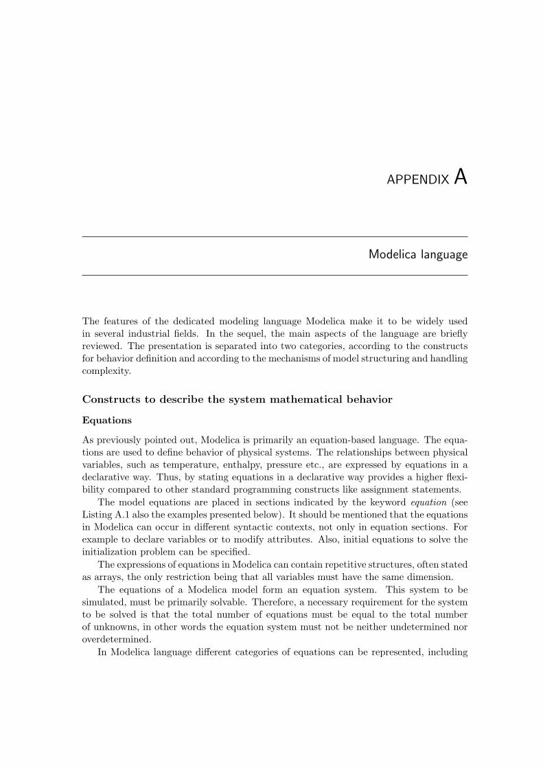
APPENDIX A
Modelica language
The features of the dedicated modeling language Modelica make it to be widely usedin several industrial fields. In the sequel, the main aspects of the language are brieflyreviewed. The presentation is separated into two categories, according to the constructsfor behavior definition and according to the mechanisms of model structuring and handlingcomplexity.
Constructs to describe the system mathematical behavior
Equations
As previously pointed out, Modelica is primarily an equation-based language. The equa-tions are used to define behavior of physical systems. The relationships between physicalvariables, such as temperature, enthalpy, pressure etc., are expressed by equations in adeclarative way. Thus, by stating equations in a declarative way provides a higher flexi-bility compared to other standard programming constructs like assignment statements.
The model equations are placed in sections indicated by the keyword equation (seeListing A.1 also the examples presented below). It should be mentioned that the equationsin Modelica can occur in different syntactic contexts, not only in equation sections. Forexample to declare variables or to modify attributes. Also, initial equations to solve theinitialization problem can be specified.
The expressions of equations in Modelica can contain repetitive structures, often statedas arrays, the only restriction being that all variables must have the same dimension.
The equations of a Modelica model form an equation system. This system to besimulated, must be primarily solvable. Therefore, a necessary requirement for the systemto be solved is that the total number of equations must be equal to the total numberof unknowns, in other words the equation system must not be neither undetermined noroverdetermined.
In Modelica language different categories of equations can be represented, including

162 Appendix: Modelica language
ordinary differential equations, algebraic equations, differential algebraic equations, dif-ference equations, hybrid DAEs and so on. Nevertheless there are a few types such aspartial differential equations that are not yet supported by the language.
Algorithms
Even if the equations are suitable to express physical phenomena, there are situationswhen the systems behavior is more conveniently represented by algorithms. A popularexample is the case when the model has to include not only the physical system but alsothe associated control system.
The algorithms, expressed as sequences of instructions (statements), can occur onlywithin the algorithm sections. As in the equations case, there is a specified keyword algo-rithm, which indicates these sections (see Listing A.2). Typically the algorithm sectionsare used when procedural descriptions are required.
In Modelica, there are different kinds of non-declarative algorithmic constructs avail-able, such as assignment statements, conditional statements(e.g. if-then-else) and itera-tion (e.g. for-loop).
equation
...
<equations >
...
<other allowed keyword >
Listing A.1: Equation section
algorithm
...
<statements >
...
<other allowed keyword >
Listing A.2: Algorithm section
Functions
The Modelica language has a limited number of predefined mathematical functions (e.g.abs, mod, sqrt, etc.). This list is completed by other functions (e.g. sin,log, exp, etc.)available in the Modelica standard library, developed together with the language by theModelica Association [7]. Also the user-defined mathematical functions are supportedby the Modelica. In general, the body of a Modelica function is represented by analgorithm section that is executed when the function is called. Each formal parameterof the functions are prefixed by either input or output keywords, the later being used toreturn the function results (see Listing A.3).
The Modelica functions calls are in general declarative1, despite the fact that theyencapsulate non-declarative constructs. The Modelica functions correspond to the math-ematical functions, meaning that for the same arguments it always returns the sameresults.
Another feature is the possibility to call functions that are defined outside of theModelica language (external functions). Thus, it enables easy reuse of tested functionsand interface with the routines of other software. The declaration of these functions ismarked with the keyword external (see Listing A.4).
1Exception: external functions called in when-equations/when statements or during initialization
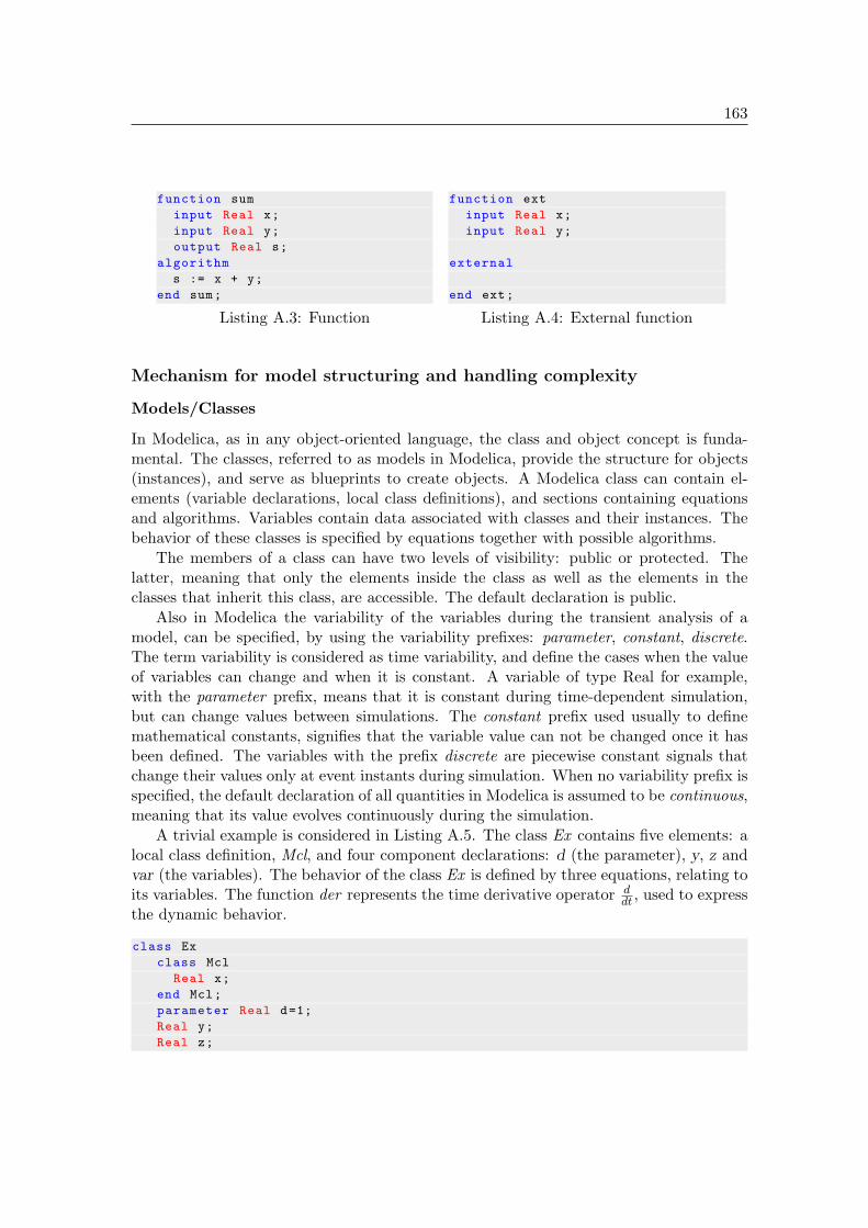
163
function sum
input Real x;
input Real y;
output Real s;
algorithm
s := x + y;
end sum;
Listing A.3: Function
function ext
input Real x;
input Real y;
external
end ext;
Listing A.4: External function
Mechanism for model structuring and handling complexity
Models/Classes
In Modelica, as in any object-oriented language, the class and object concept is funda-mental. The classes, referred to as models in Modelica, provide the structure for objects(instances), and serve as blueprints to create objects. A Modelica class can contain el-ements (variable declarations, local class definitions), and sections containing equationsand algorithms. Variables contain data associated with classes and their instances. Thebehavior of these classes is specified by equations together with possible algorithms.
The members of a class can have two levels of visibility: public or protected. Thelatter, meaning that only the elements inside the class as well as the elements in theclasses that inherit this class, are accessible. The default declaration is public.
Also in Modelica the variability of the variables during the transient analysis of amodel, can be specified, by using the variability prefixes: parameter, constant, discrete.The term variability is considered as time variability, and define the cases when the valueof variables can change and when it is constant. A variable of type Real for example,with the parameter prefix, means that it is constant during time-dependent simulation,but can change values between simulations. The constant prefix used usually to definemathematical constants, signifies that the variable value can not be changed once it hasbeen defined. The variables with the prefix discrete are piecewise constant signals thatchange their values only at event instants during simulation. When no variability prefix isspecified, the default declaration of all quantities in Modelica is assumed to be continuous,meaning that its value evolves continuously during the simulation.
A trivial example is considered in Listing A.5. The class Ex contains five elements: alocal class definition, Mcl, and four component declarations: d (the parameter), y, z andvar (the variables). The behavior of the class Ex is defined by three equations, relating toits variables. The function der represents the time derivative operator d
dt, used to express
the dynamic behavior.
class Ex
class Mcl
Real x;
end Mcl;
parameter Real d=1;
Real y;
Real z;

164 Appendix: Modelica language
Mcl var;
equation
z = d;
der(y) = y;
var.x = z;
end Ex;
Listing A.5: A class example
In Modelica, almost everything is a class. The class concept is used for differentpurposes. In order to make the programs code more accessible and easy to read andmaintain, special keywords are introduced for specific use of the class. There are severalrestricted classes (specialized), specified by keywords: model, connector, record, block,type.
A connector, is a class used to declare the structure of connection points, which maycontain variables but no equations. The model restricted class is the most widely usedtype of class for modeling purposes. Its semantics are almost the same with the generalclass concept, the only restriction is that a model may not be used in connections. A typerestricted class is usually used to introduce new type names and can be an extension toa record, an array, or one of the Modelica built-in data types: Real, Integer, Boolean,String, Enumeration. It should be noted that in Modelica all kinds of classes define types,not only the type restricted class.
Another specialized class, record, is used to declare a record data structure and maynot contain equations or algorithms. Also a class with a specified causality, is the block.The interface member variables of this class are declared by using the causality prefix,input or output.
As the restricted classes are specialized versions of the general concept of class, for avalid model, the specific keywords can be replaced by the class keyword without changingthe model behavior.
From the modeler point of view, the idea of specialized classes is useful, because it isnot necessary to learn several different concepts, but only one: the class concept. Mostof class properties, such as syntax and semantic of definition, instantiation, inheritance,genericity are the same for all kinds of specialized classes.
There are another two concepts in Modelica: package and function. These conceptsare more than restricted classes, they can be also considered as enhanced classes. Thefunction concept corresponds to the mathematical functions and its syntax and semanticsare close to the block restricted class. A package is mainly used to manage namespaces andorganize Modelica code. The packages can contain definitions of constants and all kindsof restricted classes. The requirements for a package is to not contain non-constants, i.e,parameters, variables. By using the import statement, it can get access to the definitionsof other packages.
Typing
Modelica is a strongly typed language. The strong typing in Modelica has been introducedto provide a partial verification of internal consistency, thus reducing the risk of errorsin modeling. By typing, precise data types are defined. For example, in the case of the
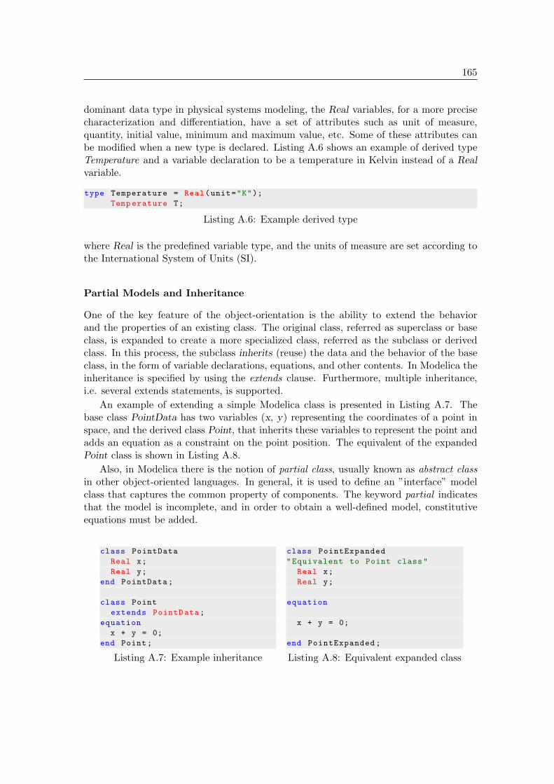
165
dominant data type in physical systems modeling, the Real variables, for a more precisecharacterization and differentiation, have a set of attributes such as unit of measure,quantity, initial value, minimum and maximum value, etc. Some of these attributes canbe modified when a new type is declared. Listing A.6 shows an example of derived typeTemperature and a variable declaration to be a temperature in Kelvin instead of a Realvariable.
type Temperature = Real(unit="K");
Temp erature T;
Listing A.6: Example derived type
where Real is the predefined variable type, and the units of measure are set according tothe International System of Units (SI).
Partial Models and Inheritance
One of the key feature of the object-orientation is the ability to extend the behaviorand the properties of an existing class. The original class, referred as superclass or baseclass, is expanded to create a more specialized class, referred as the subclass or derivedclass. In this process, the subclass inherits (reuse) the data and the behavior of the baseclass, in the form of variable declarations, equations, and other contents. In Modelica theinheritance is specified by using the extends clause. Furthermore, multiple inheritance,i.e. several extends statements, is supported.
An example of extending a simple Modelica class is presented in Listing A.7. Thebase class PointData has two variables (x, y) representing the coordinates of a point inspace, and the derived class Point, that inherits these variables to represent the point andadds an equation as a constraint on the point position. The equivalent of the expandedPoint class is shown in Listing A.8.
Also, in Modelica there is the notion of partial class, usually known as abstract classin other object-oriented languages. In general, it is used to define an ”interface” modelclass that captures the common property of components. The keyword partial indicatesthat the model is incomplete, and in order to obtain a well-defined model, constitutiveequations must be added.
class PointData
Real x;
Real y;
end PointData;
class Point
extends PointD ata;
equation
x + y = 0;
end Point;
Listing A.7: Example inheritance
class PointExpanded
"Equivalent to Point class"
Real x;
Real y;
equation
x + y = 0;
end PointExpanded;
Listing A.8: Equivalent expanded class

166 Appendix: Modelica language
Hierarchical structuring
Complex physical systems are naturally composed of several connected components, wherea part of these components can be hierarchically decomposed into distinct subcomponentsthrough multiple levels. This technique to decompose the complex models in simpler partswhich are combined in a hierarchical approach is fully supported by Modelica. Thus,an organization of structured models is performed. In order to formulate structuredmodels, the interaction between components on the same hierarchical level is achieved viaa connection mechanism, by using specialized class connector and the built-in functionconnect.
The connector class acts as an interface between components. The communicationinterface, defined by the connectors (often called ports in literature), consists of a setof variables. These variables are basically of two types: non-flow (by default) and flow(prefixed with the keyword flow). Non-flow refers to potential variables, e.g. pressure,temperature, voltage, etc., while variables of flow type usually represent some kind offlow, e.g. fluid flow rate, electrical current, force, etc.
Depending on the type of variables, two kinds of coupling, relied on laws of nature, areestablished by connections: for potential variables, these are set equal (equality coupling),while the sum of the flow variables is set to zero (sum-to-zero coupling), at the connectionpoint.
The Modelica connector classes can be used to design new interfaces and can be for-mulated for different application domains. Currently a large number of well-designedconnectors in Modelica libraries are available. The only restriction, to realize the con-nection between systems, is the fact that the components must have the same type ofconnector.
The connection between connectors are performed as equations. During translationof Modelica models, the connect statements are transformed in normal equations. Forexample, considering the Listing A.9, the Flange connector class describes an interface forinteraction in thermodynamic domain by specifying the flow variable represented by themass flow rate w and the potential variable represented by pressure p at the interactionpoint (Figure A.1).
connector Flange
Pressure p;
flow MassFlowRate w;
end Flange;
Listing A.9: Flange connector
p
w
flange
Figure A.1: A component with a flangeconnector
In Modelica there are three kinds of connection, reflecting three design situations.The first is acausal connection, when the interaction is between two physical componentsinvolving energy flow. In this case the data flow direction in connection is not explicitlyspecified. The second is causal connection, when signals (information) are exchangedbetween components. In the connector class, in this case, the data flow is specified byusing the input/output prefixes. The last type is composite connection, for the complex
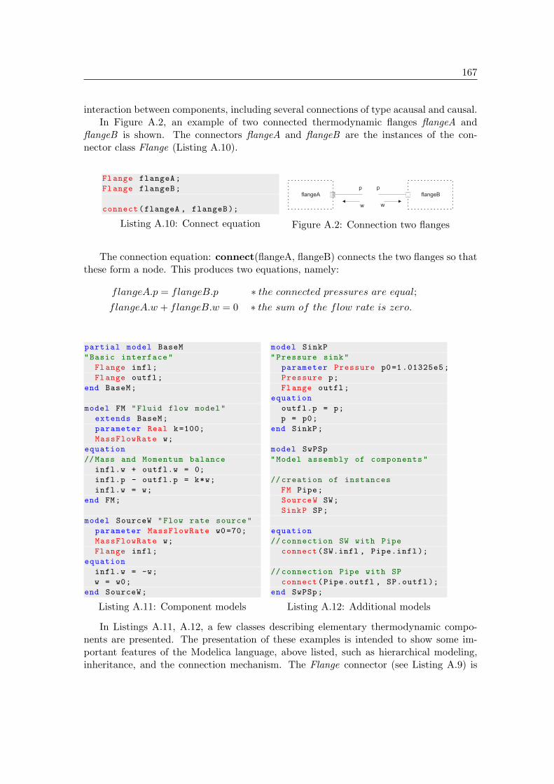
167
interaction between components, including several connections of type acausal and causal.In Figure A.2, an example of two connected thermodynamic flanges flangeA and
flangeB is shown. The connectors flangeA and flangeB are the instances of the con-nector class Flange (Listing A.10).
Flange flangeA;
Flange flangeB;
connect(flangeA , flangeB );
Listing A.10: Connect equation
p
w
p
w
flangeA flangeB
Figure A.2: Connection two flanges
The connection equation: connect(flangeA, flangeB) connects the two flanges so thatthese form a node. This produces two equations, namely:
flangeA.p = flangeB.p ∗ the connected pressures are equal;
flangeA.w + flangeB.w = 0 ∗ the sum of the flow rate is zero.
partial model BaseM
"Basic interface"
Flange infl;
Flange outfl;
end BaseM;
model FM "Fluid flow model"
extends BaseM;
parameter Real k=100;
MassFlowRate w;
equation
//Mass and Momentum balance
infl.w + outfl.w = 0;
infl.p - outfl.p = k*w;
infl.w = w;
end FM;
model SourceW "Flow rate source"
parameter MassFlowRate w0=70;
MassFlowRate w;
Flange infl;
equation
infl.w = -w;
w = w0;
end SourceW;
Listing A.11: Component models
model SinkP
"Pressure sink"
parameter Pressure p0=1 .01325e5;
Pressure p;
Flange outfl;
equation
outfl.p = p;
p = p0;
end SinkP;
model SwPSp
"Model assembly of components"
// creation of instances
FM Pipe;
SourceW SW;
SinkP SP;
equation
// connection SW with Pipe
connect(SW.infl , Pipe.infl );
// connection Pipe with SP
connect(Pipe.outfl , SP.outfl );
end SwPSp;
Listing A.12: Additional models
In Listings A.11, A.12, a few classes describing elementary thermodynamic compo-nents are presented. The presentation of these examples is intended to show some im-portant features of the Modelica language, above listed, such as hierarchical modeling,inheritance, and the connection mechanism. The Flange connector (see Listing A.9) is
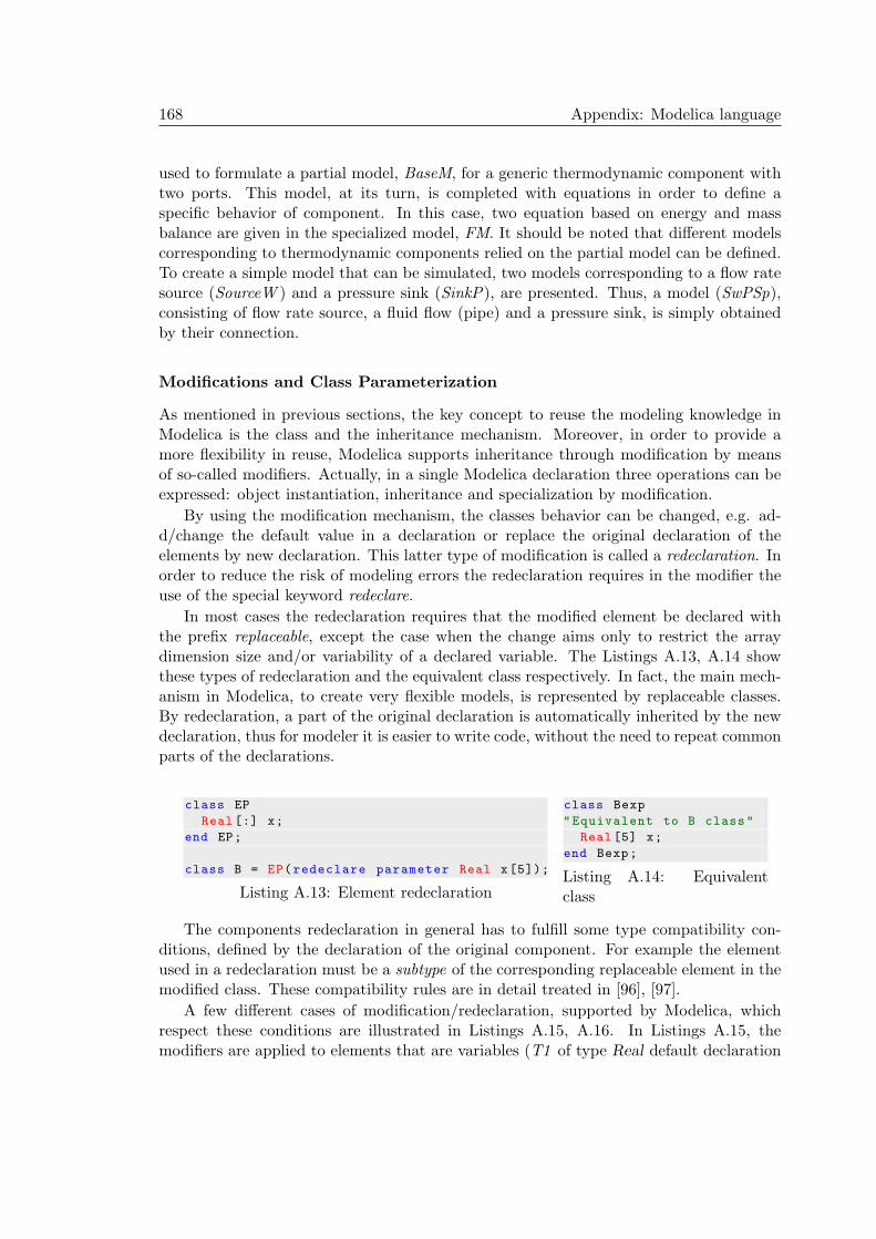
168 Appendix: Modelica language
used to formulate a partial model, BaseM, for a generic thermodynamic component withtwo ports. This model, at its turn, is completed with equations in order to define aspecific behavior of component. In this case, two equation based on energy and massbalance are given in the specialized model, FM. It should be noted that different modelscorresponding to thermodynamic components relied on the partial model can be defined.To create a simple model that can be simulated, two models corresponding to a flow ratesource (SourceW ) and a pressure sink (SinkP), are presented. Thus, a model (SwPSp),consisting of flow rate source, a fluid flow (pipe) and a pressure sink, is simply obtainedby their connection.
Modifications and Class Parameterization
As mentioned in previous sections, the key concept to reuse the modeling knowledge inModelica is the class and the inheritance mechanism. Moreover, in order to provide amore flexibility in reuse, Modelica supports inheritance through modification by meansof so-called modifiers. Actually, in a single Modelica declaration three operations can beexpressed: object instantiation, inheritance and specialization by modification.
By using the modification mechanism, the classes behavior can be changed, e.g. ad-d/change the default value in a declaration or replace the original declaration of theelements by new declaration. This latter type of modification is called a redeclaration. Inorder to reduce the risk of modeling errors the redeclaration requires in the modifier theuse of the special keyword redeclare.
In most cases the redeclaration requires that the modified element be declared withthe prefix replaceable, except the case when the change aims only to restrict the arraydimension size and/or variability of a declared variable. The Listings A.13, A.14 showthese types of redeclaration and the equivalent class respectively. In fact, the main mech-anism in Modelica, to create very flexible models, is represented by replaceable classes.By redeclaration, a part of the original declaration is automatically inherited by the newdeclaration, thus for modeler it is easier to write code, without the need to repeat commonparts of the declarations.
class EP
Real [:] x;
end EP;
class B = EP(redeclare parameter Real x[5]);
Listing A.13: Element redeclaration
class Bexp
"Equivalent to B class"
Real [5] x;
end Bexp;
Listing A.14: Equivalentclass
The components redeclaration in general has to fulfill some type compatibility con-ditions, defined by the declaration of the original component. For example the elementused in a redeclaration must be a subtype of the corresponding replaceable element in themodified class. These compatibility rules are in detail treated in [96], [97].
A few different cases of modification/redeclaration, supported by Modelica, whichrespect these conditions are illustrated in Listings A.15, A.16. In Listings A.15, themodifiers are applied to elements that are variables (T1 of type Real default declaration

169
replaced by unit=”K”), in an extends clause (the class Pex inherits the class Ppa andapplies the modifier p0=1e5, or in the case of Pbar, the modifiers are applied to the localclass Pressure within the class Ppa, changing thus the unit), hierarchical modification(the instance Ph of the class Ppa, with modified parameter, is created).
The Listing A.16 shows an example of redeclaration, redeclare MP m(x=1), thatreplace the original declaration MP m, from the class EP, and also a redeclaration of thesubtype SS, both used in an extends clause.
// Modifier to variable
Real T(unit="K");
class Ppa
type Pressu re = Real(unit="Pa");
Pressure P;
parameter Real p0;
end Ppa;
//to local class
class Pbar
extends Ppa(Pressu re(unit="bar"));
end Pbar;
// nested extends clause
class Pex
extends Ppa(p0=1e5);
end Pex;
// hierarchical
Ppa Ph(p0(unit="bar") = 1);
Listing A.15: Modification examples
// Redeclaration
class MP
parameter Real x;
end MP;
class SS "subtype of MP"
parameter Real x=10;
parameter Real y;
end SS;
class EP
replaceable MP m;
end EP;
class EPs
extends EP(redeclare MP m(x=1));
end EPs;
class EM
extends EP(redeclare SS m(y=1));
end EM;
Listing A.16: Redeclaration examples
The redeclaration approach enables the use of the parametrized generic classes, com-monly known as generics. Instead to write code for several similar models, a significantamount of coding as well as software maintenance can be reduced by expressing a generalstructure of the problem (”prototype model”), with specific information provided as for-mal parameters. The formal class parameters makes from Modelica a flexible modelinglanguage, thus depending on situation and purpose, simplified models can be refined intoa high precision models, by exchanging sub-models or even whole sub-systems.
In Modelica two cases of class parameterization can be noted: formal class parametersare components (i.e. when objects are used as values) or types (i.e. when types are used asvalues). In Listing A.17, the first case when class parameters are variables (components)is presented.
Consider the description of the thermodynamic circuit (SwPSp), previously presentedin Listing A.12. In this case, SwPSp has a formal class parameter Pipe (components ofSwPSp), marked by the keyword replaceable, and two components SW, SP that are notclass parameters because are not declared replaceable.
Assuming that there is a more detailed model of the fluid flow, FMc, subtype of FM,the target is to create a model (called C), with the same structure but containing FMc.

170 Appendix: Modelica language
This is easily performed, by exchanging the FM with the new model, FMc, in other words,the default declaration of the class parameter Pipe is changed in the definition of the classC. The equivalent of this class is also illustrated (CC).
An example relating to the second case, when the class parameters are types, is shownin Listing A.18. Considering this example, it is possible to change a set of models bydefining a type parameter Mr in the generic model SwPSp, all objects having this typecan be then changed (e.g. from the default type FM to FMc type).
model SwPSp
replaceable FM Pipe;
SourceW SW;
SinkP SP;
equation
...
end SwPSp;
model C = SwPSp(redeclare FMc Pipe);
//class equivalent to C
model CC
FMc Pipe;
SourceW SW;
SinkP SP ;
equation
...
end CC;
Listing A.17: Modification examples
model SwPSp
replaceable model Mr=FM;
Mr Pipe;
SourceW SW;
SinkP SP ;
equation
...
end SwPSp;
model C = SwPSp(redeclare Mr=FMc);
//class equivalent to C
model CC
FMc Pipe;
SourceW SW;
SinkP SP ;
equation
...
end CC;
Listing A.18: Redeclaration examples
Annotations
Apart from the features above mentioned, Modelica provides a particular construction,called annotation, to store additional information about the elements of the models. Thisfeature is used by Modelica environments for example to describe a graphical representa-tion of the icons and connections associated with models or to support model documen-tation. In general, the annotations are widely used by library developers. By graphicalrepresentation, the models become easier to understand, and the users can create modelsbased on elements of libraries, in a drag and drop manner, without directly working withthe Modelica code. The graphical annotations are also represented textually in the modelcode, thus making possible a textual editing. This is seldom made because most toolsprovide a graphical modeling environment. In addition, in Modelica language, specialannotations can be defined for functions, in order to obtain a higher performance and/ornumerical accuracy.

APPENDIX B
Modelica tools
Currently there are several software tools for physical system modeling based on the open-source standard Modelica. Some such tools are briefly presented in the following, for moreinformation, see [7].
Generally any Modelica environment needs to contain the following modules:
• a Modelica compiler (interpreter), that translates the Modelica model into a formwhich can be efficiently simulated. Symbolic manipulation algorithms are required;
• an execution and run-time system, to simulate the translated model with standardnumerical solvers and plotting of the results;
• a text editor for models editing, that can be a specialized Modelica or any standardtext editor;
• a graphical editor for graphical representation of models and browsing.
These features can be found in different variants in all Modelica tools presented in thefollowing lines.
Dymola
Dymola, Dynamic Modeling Laboratory [8], is a modeling and simulation environmentbased on Modelica language. Dymola provides a powerful Modelica translator that is ableto perform symbolic manipulation for large-scale systems (more than 100 000 equations),as well as for real-time applications, currently being considered the leading Modelica soft-ware. Apart from the common features above listed, graphical model editing, simulationand plotting, Dymola enables model calibration, parameter optimization and real-timeHardware in the Loop Simulations (HILS). In addition, Dymola can be connected withMatlab by means of Dymola-Symulink interface (DymolaBlock). Dymola offers also a

172 Appendix: Modelica tools
wide range of libraries, covering different engineering domains (e.g. mechanical, elec-trical, thermodynamical, etc.), with the open possibility of the user to create modelsaccording to their specific needs, using the templates and elements from these libraries.
OpenModelica
The OpenModelica [140] is an open source project that supports the full Modelica lan-guage but with a lower level of efficiency, in terms of computation and solving the equa-tions systems, than Dymola. OpenModelica uses MetaModelica, an extension of theModelica specifically designed to expand the tool functionality.
MathModelica
MathModelica [141] is a commercial Modelica environment relied on the integration ofModelica with the Mathematica language. The subset Modelica is used for object-orientedmodeling and simulation whereas the Mathematica part is used for interactive scripting,providing extensibility and flexibility in functionality. MathModelica provides a customiz-able set of Modelica component libraries but with a reduced number compared to Dymola.
MapleSim
MapleSim [142] is a multi-domain modeling and simulation tool, supporting Modelica.MapleSim combines Modelica libraries with advanced symbolic computing technologyand high-performance numerical solvers, taking advantage of Maple’s features.
SimulationX
SimulationX [143] is a graphically-interactive tool for modeling, simulation and analysisof multi-domain systems. The whole range of the SimulationX computation methods,can be applied to all kinds of Modelica models. SimulationX offers also the possibility toexport models to various platforms such as Matlab/Simulink, dSPACE, Simpack etc.
This section presents only a few most popular environments with different levels of sup-port for Modelica, the list goes on. As the adoption of Modelica as standard for dynamicmodeling is steadily increasing, in the near future, it is expected that the level of supportas well as the number of tools for Modelica to increase.
JModelica.org
The project is described as an extensible Modelica-based open source platform for opti-mization, simulation and analysis of complex dynamic systems. JModelica.org tries to fillthe gap between modeling/simulation tools and the numerical optimization algorithms.Effectively, the platform enables a high-level description of the models, simulation, analy-sis and optimization, in a fully integrated way. The formulation of dynamic optimizationproblems is performed into an extension of the Modelica language, called Optimica [144].This extension complements Modelica with language constructs dedicated to optimization

173
(e.g. cost functions, constraints, quantities to optimize), enabling the user to use high-level descriptions to express optimization problems. As a key feature of the Optimica isthe fact that the formulation of the optimization problem is performed independently ofthe numerical algorithm used to solve the problem. The algorithm and associated controlparameters can be specified using language constructs, making easy the applicability ofdifferent algorithms. The JModelica.org platform implements state of the art numericalalgorithms e.g. simultaneous optimization method based on Lagrange polynomials onfinite element with Radau points. In particular, Jacobians and sparsity information areexploited in order to increase the efficiency of the algorithm. The non-linear programresulting from collocation is then solved by the solver IPOPT.
Currently the platform is under development, with several constraints on the modelsformulation, complexity and syntax, limitations which are highlighted in the content ofthis thesis, limitations that have made our attempt to use this environment to deal withthe start-up optimization problem based on the developed CCPP models to fail.

APPENDIX C
CCPP identified model
A solution to derive simple models of combined cycle power plant suitable for controlpurposes is to use an identification/interpolation procedure. The principle of the methodis here presented.
Identification and interpolation procedure 1
According to the approach proposed in [145], [146], the nonlinear combined cycle modelcan be considered as composed by a number of local linear identified models combinedby means of a scheduling variable, which describes their local validity through suitablydefined membership functions. As in the start-up phase one of the most important vari-ables is represented by the load level signal GTLoad, this has been selected as schedulingvariable, i.e. the variable specifying the current operating condition. The Modelica de-veloped model has been integrated in Matlab by using Dymola-Simulink interface, andseveral transients to identify models for different operating points have been generated.The identification of each simulation transient has been performed by means of the MatlabSystem Identification Toolbox [147]. The considered approach is based on the followingmain steps:
I. Consider that the operating set of the model is partitioned into n (n=10) disjointoperating regimes. To each regime corresponds a significant value of the GTLoad.According to the normal functioning of this type of plant, the selected plant oper-ating points are:
• 7.5% of full load;
• 15% of full load;
• 25% of full load;
• 40% of full load;
• 50% of full load;
• 57% of full load;
• 60% of full load;
• 65% of full load;
• 75% of full load;
• 100% of full load.
1Work carried out in collaboration with Dipartimento di Elettronica e Informazione, Politecnico diMilano

176 Appendix: CCPP identified model
It should be noted that this set of values has been selected to cover the overalloperating range of the system and is more dense around 60% where the plant modelexhibits a strongly nonlinear behaviour.
II. In order to generate appropriate identification data, different simulations of theDymola/Modelica model, with small step variations around each operating pointof the interest variable, have been performed. For the determination of the steadystate conditions at any point, the Dymola simulator has been used. It should benoted that in the case of the CCPP system, the model to be identified has beeninitialized in a state corresponding to a hot start-up phase and has three signalsof interest: GT level load, ST throttle valve position and the desuperheater flowrate. The drum feed-water flow rate is controlled by a local regulator to avoid theproblems of an excessive increase/decrease of the level inside the drum, while theother inputs: the bypass position and the grid breaker are maintained constant,with the bypass valve completely closed and the ST connected to the grid.
III. The generated data have been subsequently used to identify linear models withlocal validity. Thus, a local model (Mi, with i = 1, ..., n) has been associated toeach operating regime. These models have been estimated by means of standardidentification procedures (e.g. based on the Least Squares method), using ARX(AutoRegressive with eXogenous variable) and OE (Output Error) structures. Ingeneral the use of first and/or second order models are adequate to describe thetransients of the outputs with satisfactory results for the proposed purposes. Forexample, the comparison between the transients corresponding to the simulationdata model with those provided by the estimated model, when a step positive varia-tion of the GTLoad at the 75% of its nominal value is applied, are shown in FiguresC.1a and C.1b. As it can be seen, the obtained responses with the two models, inthe case of two interest variables during start-up, steam temperature and headerstress, are quite close, showing thus the consistency of the identified model.
IV. Once the local linear models have been estimated, the overall identified plant model(M) has been obtained by suitably interpolating at any operating point the locallinear models through the use of weights:
M =n∑
i=1
µi(φ)Mi (C.1a)
µi(φ) ∈[0, 1] (C.1b)
n∑
i=1
µi(φ) = 1, ∀φ ∈ Π (C.1c)
where φ represents the scheduling variable, GTLoad, chosen to cover if possible theoverall operating set of the system (Π) and µi denotes the weighting functions whichdefine the validity of the local estimated models. The weights have been specified by
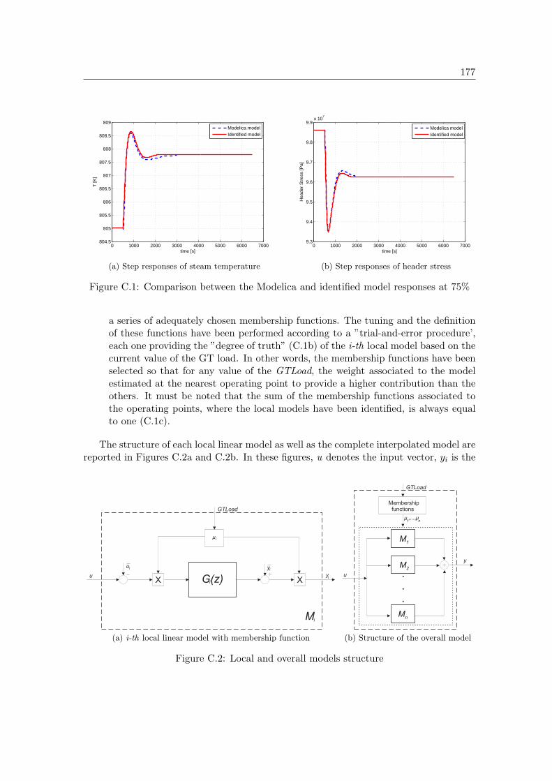
177
0 1000 2000 3000 4000 5000 6000 7000804.5
805
805.5
806
806.5
807
807.5
808
808.5
809
time [s]
T [K
]
Modelica modelIdentified model
(a) Step responses of steam temperature
0 1000 2000 3000 4000 5000 6000 70009.3
9.4
9.5
9.6
9.7
9.8
9.9x 10
7
time [s]
Hea
der
Str
ess
[Pa]
Modelica modelIdentified model
(b) Step responses of header stress
Figure C.1: Comparison between the Modelica and identified model responses at 75%
a series of adequately chosen membership functions. The tuning and the definitionof these functions have been performed according to a ”trial-and-error procedure’,each one providing the ”degree of truth” (C.1b) of the i-th local model based on thecurrent value of the GT load. In other words, the membership functions have beenselected so that for any value of the GTLoad, the weight associated to the modelestimated at the nearest operating point to provide a higher contribution than theothers. It must be noted that the sum of the membership functions associated tothe operating points, where the local models have been identified, is always equalto one (C.1c).
The structure of each local linear model as well as the complete interpolated model arereported in Figures C.2a and C.2b. In these figures, u denotes the input vector, yi is the
X XG(z)
GTLoad
M
u
u y
y
i i
i
i
i
(a) i-th local linear model with membership function
GTLoad
Membershipfunctions
M1
M2
Mn
.
.
.
u
y
1 n,...,
(b) Structure of the overall model
Figure C.2: Local and overall models structure

178 Appendix: CCPP identified model
output of the local model Mi, Gi(z) is the identified transfer function of the local linearmodel, (ui, yi) is the input-output equilibrium pair for the i-th working point specified bythe corresponding value of the GTLoad and y represents the output of the overall modelobtained as the sum of the outputs yi, i = 1, ..., n of the local models Mi.
The consistency of the model developed by the identification and interpolation proce-dure has been tested in several simulation scenarios. In addition to the local comparisonof responses generated by each identified model with those provided by the Modelicasimulator, several large transients have been performed. The results of such a scenariowhen a wide ramp variation of the GTLoad (from 100% to the 15% of the nominal load)is applied, are reported in Figures C.3a and C.3b.
0 1 2 3 4 5 6 7
x 104
600
650
700
750
800
850
time [s]
T [K
]
Modelica modelIdentified model
(a) Steam temperature responses
0 1 2 3 4 5 6 7
x 104
6.5
7
7.5
8
8.5
9
9.5
10
10.5
11x 10
7
time [s]
Hea
der
Str
ess
[Pa]
Modelica modelIdentified model
(b) Header stress responses
Figure C.3: Comparison between the Modelica and identified model responses correspond-ing to a large transient (from 100% to the 15% of the GT nominal load))
It is apparent that the identified model can reproduce the plant dynamics of interestwith satisfactory accuracy, both for local and for large variations of the working point.The only variable that requires a deeper investigation is represented by the rotor stressof the ST, that according to the results given by an optimization procedure exhibitsan incompatibility between the real simulator behavior and the one obtained with theidentified model. This is probably due to the insufficient accuracy of the identified modelfor the rotor stress variable, and as a possible solution, a more appropriate identificationof the stress model in the rotor section has to be done.
Concerning the adopted procedure to obtain the interpolated identified model, thenumber of operating points is important but it must be emphasized that the most cum-bersome and time consuming phase concerns the definition and tuning of the membershipfunctions. In this regard, automatic procedures based, e.g., on the optimization of thequality of the open-loop simulation results over large transients could be conceived to re-duce the development time. Furthermore, a direct analysis of a classical start-up transientto tune the membership functions can be envisaged.
Concluding, the proposed method appears to provide promising results. Typically,the method performance depends strongly on the quality of the identified linear models

179
as well as on the membership functions specification. The procedure can be furtherimproved, in particular with an optimized selection of the membership functions andwith the consideration of the other signals (e.g. throttle valve position and desuperheaterflow rate). Indeed, the later will require a more complete procedure that deals with thedefinition of the operating points where to perform local model identification and thesubsequent optimization of the corresponding membership functions.


APPENDIXD
Structure of the ThermoOpt library
The optimization-oriented model components developed in this dissertation have beenincluded in the ThermoOpt library.
The ThermoOpt library is composed of 7 main packages and 2 auxiliary packages.The overall structure of the ThermoOpt library is shown in Figure D.1.
Figure D.1: Structure of the ThermoOpt library

182 Appendix: Structure of the ThermoOpt library
Package CCPP
The package CCPP contains the models of the main units of the plant: GT, HRSG, ST.The package includes also two sub-packages: Buses and Control. The sub-package Buseshas bus definitions (empty connectors defined by expansion) used to make the connectionssimpler for users. The package Control has a block model which can provide P, PI, PD,and PID controllers with anti-windup
Package Media
The package Media contains two sub-packages: Water and FlueGasSingle. The packageWater provides a water/steam properties model developed according to the smoothnessrequirements, while the package FlueGasSingle provides a medium model for a typicalgas turbine exhaust, also adapted to the optimization requirements.
Package Water
The provides models of components that use water/steam as working fluid. The packagecontains models of elementary components such as valves, pumps, mixers, headers, drumboilers, ideal flow sources, turbines, etc.
Package Gas
The package Gas provides models of components that use ideal gases as working fluid.Similarly to the Water, this package contains models of elementary components.
Package Thermal
The Thermal package includes basic modeling blocks to describe heat transfer phenomena.
Package Electrical
The Electrical package contains idealized models of electric power components.
Package Functions
The Functions package includes several functions used to describe behavior of subsystemsor for a smooth approximation (e.g., the smooth approximation of the abs and maxfunctions).
Package Sequences
The package Sequences contains several shutdown and start-up sequences used in thephases of validation and initialization of the CCPP model.
Package Test
The package Test contains a few test cases for the component models of the library.
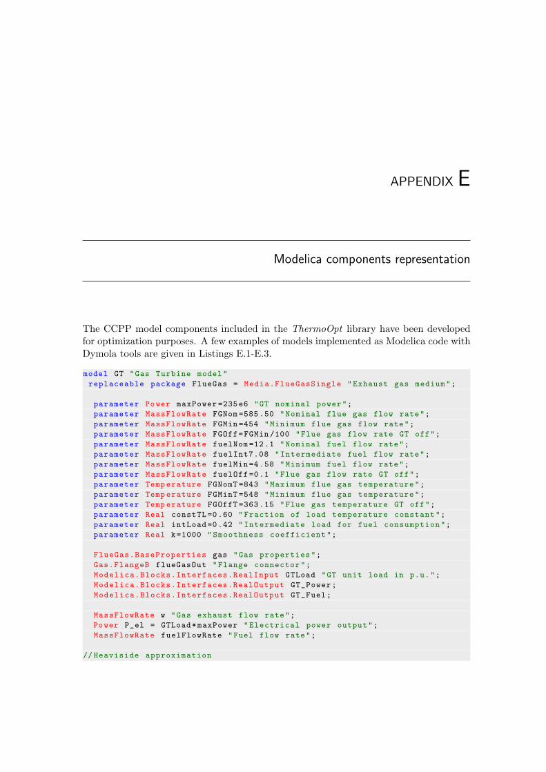
APPENDIX E
Modelica components representation
The CCPP model components included in the ThermoOpt library have been developedfor optimization purposes. A few examples of models implemented as Modelica code withDymola tools are given in Listings E.1-E.3.
model GT "Gas Turbine model"
replaceable package FlueGas = Media.FlueGasSingle "Exhaust gas medium";
parameter Power maxPower =235e6 "GT nominal power";
parameter MassFlowRate FGNom =585 .50 "Nominal flue gas flow rate";
parameter MassFlowRate FGMin =454 "Minimum flue gas flow rate";
parameter MassFlowRate FGOff=FGMin /100 "Flue gas flow rate GT off";
parameter MassFlowRate fuelNom =12.1 "Nominal fuel flow rate";
parameter MassFlowRate fuelInt7.08 "Intermediate fuel flow rate";
parameter MassFlowRate fuelMin =4.58 "Minimum fuel flow rate";
parameter MassFlowRate fuelOff =0.1 "Flue gas flow rate GT off";
parameter Temp erature FGNomT =843 "Maximum flue gas temperature";
parameter Temp erature FGMinT =548 "Minimum flue gas temperature";
parameter Temp erature FGOffT =363 .15 "Flue gas temperature GT off";
parameter Real constTL =0.60 "Fraction of load temperature constant";
parameter Real intLoad =0.42 "Intermediate load for fuel consumption";
parameter Real k=1000 "Smoothness coefficient";
FlueGas.BaseProperties gas "Gas properties";
Gas.FlangeB flueGasOut "Flange connector";
Modelica.Blocks.Interfaces.RealInput GTLoad "GT unit load in p.u.";
Modelica.Blocks.Interfaces.RealOutput GT_Power;
Modelica.Blocks.Interfaces.RealOutput GT_Fuel;
MassFlowRate w "Gas exhaust flow rate";
Power P_el = GTLoad*maxPower "Electrical power output";
MassFlowRate fuelFlowRate "Fuel flow rate";
// Heaviside approximation
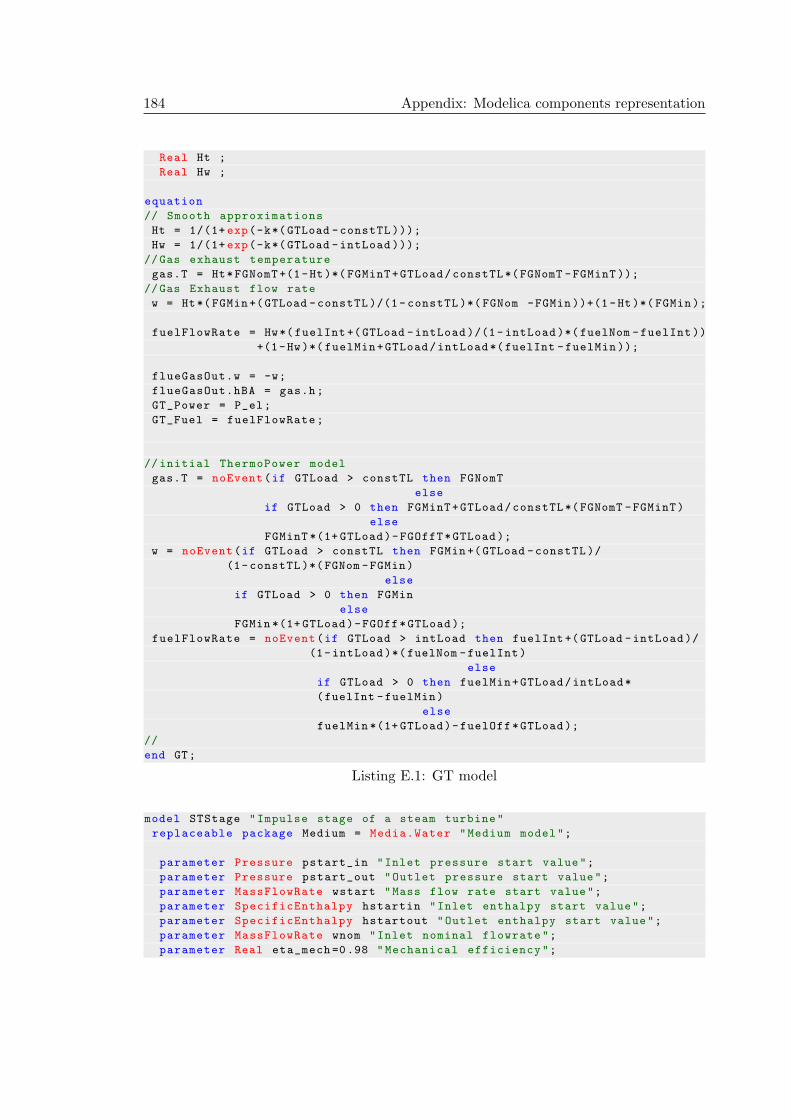
184 Appendix: Modelica components representation
Real Ht ;
Real Hw ;
equation
// Smooth approximations
Ht = 1/(1+ exp(-k*(GTLoad -constTL )));
Hw = 1/(1+ exp(-k*(GTLoad -intLoad )));
//Gas exhaust temperature
gas.T = Ht*FGNomT +(1-Ht)*( FGMinT+GTLoad/constTL *(FGNomT -FGMinT ));
//Gas Exhaust flow rate
w = Ht*( FGMin +(GTLoad -constTL )/(1- constTL )*( FGNom -FGMin ))+(1 -Ht)*( FGMin );
fuelFlowRate = Hw*( fuelInt +(GTLoad -intLoad )/(1- intLoad )*( fuelNom -fuelInt ))
+(1-Hw)*( fuelMin+GTLoad/intLoad *(fuelInt -fuelMin ));
flueGasOut.w = -w;
flueGasOut.hBA = gas.h;
GT_Power = P_el;
GT_Fuel = fuelFlowRate;
// initial ThermoPower model
gas.T = noEvent(if GTLoad > constTL then FGNomT
else
if GTLoad > 0 then FGMinT+GTLoad/constTL *(FGNomT -FGMinT)
else
FGMinT *(1+ GTLoad)-FGOffT*GTLoad );
w = noEvent(if GTLoad > constTL then FGMin +(GTLoad -constTL )/
(1-constTL )*(FGNom -FGMin)
else
if GTLoad > 0 then FGMin
else
FGMin *(1+ GTLoad)-FGOff*GTLoad );
fuelFlowRate = noEvent(if GTLoad > intLoad then fuelInt +(GTLoad -intLoad )/
(1-intLoad )*( fuelNom -fuelInt)
else
if GTLoad > 0 then fuelMin+GTLoad/intLoad*
(fuelInt -fuelMin)
else
fuelMin *(1+ GTLoad)-fuelOff*GTLoad );
//
end GT;
Listing E.1: GT model
model STStage "Impulse stage of a steam turbine"
replaceable package Medium = Media.Water "Medium model";
parameter Pressure pstart_in "Inlet pressure start value";
parameter Pressure pstart_out "Outlet pressure start value";
parameter MassFlowRate wstart "Mass flow rate start value";
parameter SpecificEnthalpy hstartin "Inlet enthalpy start value";
parameter SpecificEnthalpy hstartout "Outlet enthalpy start value";
parameter MassFlowRate wnom "Inlet nominal flowrate";
parameter Real eta_mech =0.98 "Mechanical efficiency";
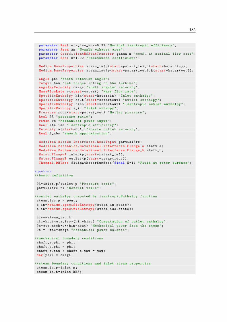
185
parameter Real eta_iso_nom =0.92 "Nominal isentropic efficiency";
parameter Area An "Nozzle exhaust area";
parameter CoefficientOfHeatTransfer gamma_n "coef. at nominal flow rate";
parameter Real k=1000 "Smoothness coefficient";
Medium.BaseProperties steam_in(p(start=pstart_in),h(start=hstartin ));
Medium.BaseProperties steam_iso(p(start=pstart_out),h(start=hstartout ));
Angle phi "shaft rotation angle";
Torque tau "net torque acting on the turbine";
AngularVelocity omega "shaft angular velocity";
MassFlowRate w(start=wstart) "Mass flow rate";
SpecificEnthalpy hin(start=hstartin) "Inlet enthalpy";
SpecificEnthalpy hout(start=hstartout) "Outlet enthalpy";
SpecificEnthalpy hiso(start=hstartout) "Isentropic outlet enthalpy";
SpecificEntropy s_in "Inlet entropy";
Pressure pout(start=pstart_out) "Outlet pressure";
Real PR "pressure ratio";
Power Pm "Mechanical power input";
Real eta_iso "Isentropic efficiency";
Velocity u(start =0.1) "Nozzle outlet velocity";
Real S_abs "smooth approximation";
Modelica.Blocks.Interfaces.RealInput partialArc;
Modelica.Mechanics.Rotational.Interfaces.Flange_a shaft_a;
Modelica.Mechanics.Rotational.Interfaces.Flange_b shaft_b;
Water.FlangeA inlet(p(start=pstart_in ));
Water.FlangeB outlet(p(start=pstart_out ));
Thermal.DHThtc fluidAtRotorSurface (final N=1) "Fluid at rotor surface";
equation
//basic definition
PR=inlet.p/outlet.p "Pressure ratio";
partialArc =1 "Default value";
// outlet enthalpy computed by isentropicEnthalpy function
steam_iso.p = pout;
s_in=Medium.specificEntropy(steam_in.state );
s_in=Medium.specificEntropy(steam_iso.state );
hiso=steam_iso.h;
hin -hout=eta_iso *(hin -hiso) "Computation of outlet enthalpy";
Pm=eta_mech*w*(hin -hout) "Mechanical power from the steam";
Pm = -tau*omega "Mechanical power balance";
// mechanical boundary conditions
shaft_a.phi = phi;
shaft_b.phi = phi;
shaft_a.tau + shaft_b.tau = tau;
der(phi) = omega;
//steam boundary conditions and inlet steam properties
steam_in.p=inlet.p;
steam_in.h=inlet.hBA;

186 Appendix: Modelica components representation
hin=steam_in.h;
hout=outlet.hBA;
pout=outlet.p;
w = inlet.w;
inlet.w + outlet.w = 0 "Mass balance";
inlet.hAB = outlet.hBA "Close balance equation";
// impulse stage description
eta_iso = eta_iso_nom "Constant efficiency";
hin = hiso + u^2/2;
w = steam_iso.d*An*u;
fluidAtRotorSurface.T [1] = steam_iso.T "Fluid temp. at rotor surface";
// initial ThermoPower model
// /////////////////////////
fluidAtRotorSurface.gamma [1] = gamma_n *(abs(w)/wnom )^0.8 "heat transfer";
// ////////////////////////
// replaced by
S_abs =(((2*w)^2+k^2)^0 .5)/2;
fluidAtRotorSurface.gamma [1] = gamma_n *( S_abs/wnom )^0.8 "heat transfer";
end STStage;
Listing E.2: ST impulse stage model
model Condenser "Pressure sink for water/steam flows"
extends Icons.Water.SourceP ;
replaceable package Medium = Media.Water "Medium model";
parameter Pressure p0=1 .01325e5 "Nominal pressure";
parameter Pressure pmin=0.1e5 "Minimum pressure";
parameter Pressure pmax=0 .15e5 "Maximum pressure";
parameter MassFlowRate wmin =18 "Minimum flow";
parameter MassFlowRate wmax =82.5 "Maximum flow";
parameter SpecificEnthalpy h=1e5 "Nominal specific enthalpy";
Pressure p;
Modelica.Blocks.Interfaces.RealInput in_w;
Water.FlangeA flange;
equation
flange.p = p;
p = ((pmax -pmin )/(wmax -wmin ))* in_w;
flange.hAB =h;
end Condenser;
Listing E.3: Condenser model

APPENDIX F
CCPP Dymola diagram
The CCPP model presented throughout this manuscript has been developed in the Dy-mola environment. The model corresponds to a combined cycle plant with one single levelof pressure and includes the following units:
• Gas Turbine;
• Heat Recovery Steam Generator:
– 1 drum boiler;
– 3 heat exchangers;
– 1 desuperheater system (Mixer + water source);
– 1 steam header;
• Steam line;
• Steam Turbine:
– turbine;
– bypass/valve circuit;
– rotational inertia of the turbine;
– electrical generator;
– power grid;
• Condenser.
The Dymola representation of the plant model with the main components is presentedin Figures F.1a-F.2b. It should be pointed out that in the case of optimization-orientedmodel the steam line unit has not been included in the structure of the system.

188 Appendix: CCPP Dymola diagram
(a) Plant implementation as Dymola/Modelica model
(b) Structure of the plant model
Figure F.1: Structure of the CCPP model represented in Dymola
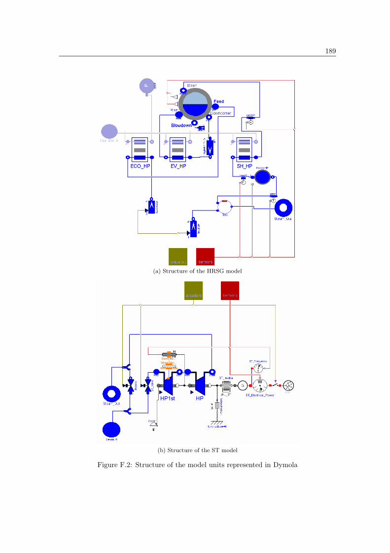
189
(a) Structure of the HRSG model
(b) Structure of the ST model
Figure F.2: Structure of the model units represented in Dymola


APPENDIX G
Execution of Modelica/Dymola model in Matlab
For optimization and control designed, the smooth CCPP model developed in Modeli-ca/Dymola has been imported in Matlab by means of Dymola-Matlab interface.
Dymola-Matlab interface
Dymola provides convenient interfaces to Matlab and to the simulation and modelingplatform Simulink. It enables to combine the powerful physical modeling capabilitiesof Modelica language with efficient tools for control design and optimization given byMatlab.
In addition to the fact that a model can be transformed into a S-function file andsimulated in Simulink as an input/output block, Dymola compiles the model into anexecutable Dymosim file (dymosim.exe). Dymosim contains the code necessary for con-tinuous simulation, and event handling. Model descriptions are compiled into machinecode such that to reach maximum execution speed during simulation. The dymosim is astand-alone application which can be used in several different environments.
Dymosim has no graphical user interface, and reads the experiment description froman input file, performs a simulation run, stores the result into an output file and termi-nates. The dymosim executable can be directly called by user from Matlab:
>>dos(’dymosim.exe’);
or as a m-function :
>> [s,n] = dymosim(exp,x0,p);
The simulation run of the Dymola model is performed by reading an input file ’dsin.txt ’with the initial state, by storing the simulation result into the binary file ’dsres.mat ’, andoptionally by loading the result from file into ’s, n’. The executable ’dymosim’ contains
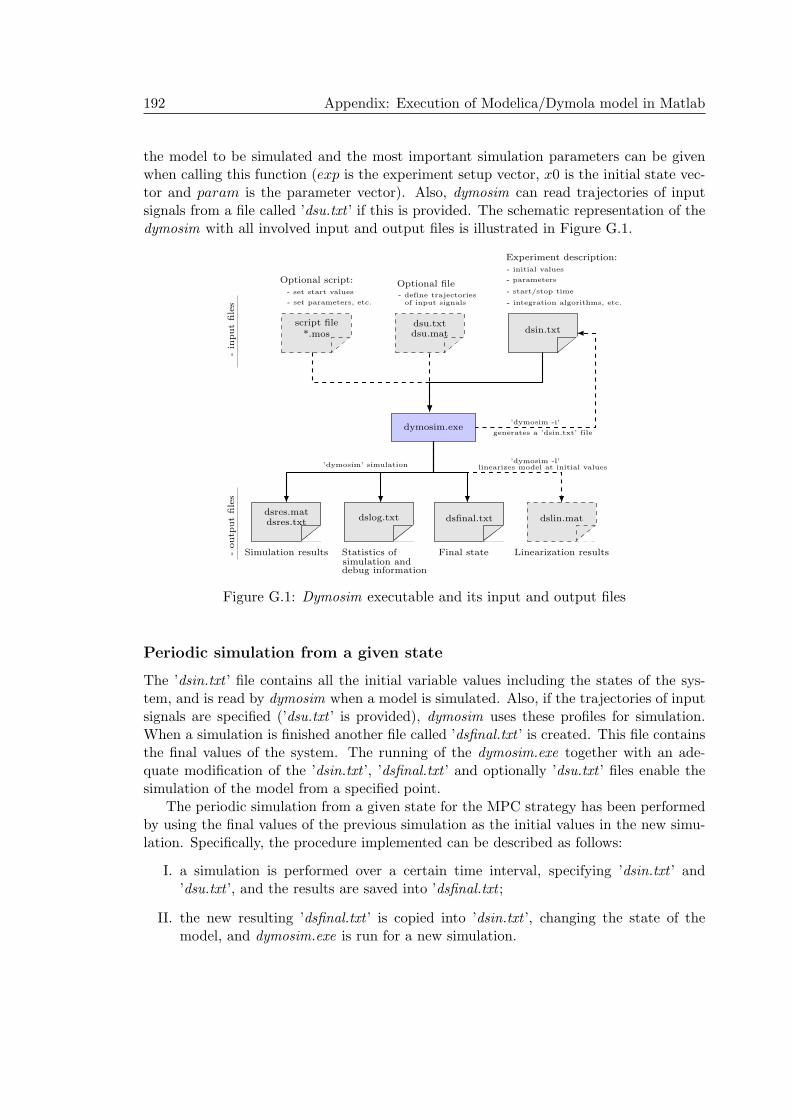
192 Appendix: Execution of Modelica/Dymola model in Matlab
the model to be simulated and the most important simulation parameters can be givenwhen calling this function (exp is the experiment setup vector, x0 is the initial state vec-tor and param is the parameter vector). Also, dymosim can read trajectories of inputsignals from a file called ’dsu.txt ’ if this is provided. The schematic representation of thedymosim with all involved input and output files is illustrated in Figure G.1.
dsres.matdsres.txt
dslog.txt dsfinal.txt dslin.mat
script file
*.mosdsu.txtdsu.mat dsin.txt
Simulation results Statistics ofsimulation anddebug information
Final state Linearization results
’dymosim -l’linearizes model at initial values
’dymosim -i’
generates a ’dsin.txt’ file
’dymosim’ simulation
dymosim.exe
Experiment description:
- initial values
- parameters
- start/stop time
- integration algorithms, etc.
Optional file- define trajectoriesof input signals
Optional script:
- set start values
- set parameters, etc.
-inputfiles
-outp
utfiles
Figure G.1: Dymosim executable and its input and output files
Periodic simulation from a given state
The ’dsin.txt ’ file contains all the initial variable values including the states of the sys-tem, and is read by dymosim when a model is simulated. Also, if the trajectories of inputsignals are specified (’dsu.txt ’ is provided), dymosim uses these profiles for simulation.When a simulation is finished another file called ’dsfinal.txt ’ is created. This file containsthe final values of the system. The running of the dymosim.exe together with an ade-quate modification of the ’dsin.txt ’, ’dsfinal.txt ’ and optionally ’dsu.txt ’ files enable thesimulation of the model from a specified point.
The periodic simulation from a given state for the MPC strategy has been performedby using the final values of the previous simulation as the initial values in the new simu-lation. Specifically, the procedure implemented can be described as follows:
I. a simulation is performed over a certain time interval, specifying ’dsin.txt ’ and’dsu.txt ’, and the results are saved into ’dsfinal.txt ;
II. the new resulting ’dsfinal.txt ’ is copied into ’dsin.txt ’, changing the state of themodel, and dymosim.exe is run for a new simulation.

List of Figures
1 Schema d’une centrale a cycles combines de type 1-1-1 . . . . . . . . . . . xiii2 La fonction de Heaviside et son approximation pour k=20 . . . . . . . . . xvi3 Reponses comparatives . . . . . . . . . . . . . . . . . . . . . . . . . . . . . xviii4 Resultats comparatifs de simulation . . . . . . . . . . . . . . . . . . . . . xxi
1.1 World primary energy demand by fuel according IEA scenario . . . . . . . 61.2 World electricity production 2008: partition by primary energy sources . . 71.3 France electricity production 2008: partition by primary energy sources . 8
2.1 Schematic of a combined cycle type 1-1-1 . . . . . . . . . . . . . . . . . . 192.2 Gas turbine structure . . . . . . . . . . . . . . . . . . . . . . . . . . . . . 202.3 Gas turbine . . . . . . . . . . . . . . . . . . . . . . . . . . . . . . . . . . . 212.4 Launch mode of the Gas turbine . . . . . . . . . . . . . . . . . . . . . . . 212.5 Heat Recovery Steam Generator with one pressure level . . . . . . . . . . 222.6 HSRG decomposition . . . . . . . . . . . . . . . . . . . . . . . . . . . . . . 232.7 HRSG with 3 pressure levels and reheat . . . . . . . . . . . . . . . . . . . 242.8 HP circuit . . . . . . . . . . . . . . . . . . . . . . . . . . . . . . . . . . . . 262.9 IP circuit . . . . . . . . . . . . . . . . . . . . . . . . . . . . . . . . . . . . 262.10 LP circuit . . . . . . . . . . . . . . . . . . . . . . . . . . . . . . . . . . . . 272.11 SL schematic representation . . . . . . . . . . . . . . . . . . . . . . . . . . 282.12 Schematic diagram of multi-stage ST . . . . . . . . . . . . . . . . . . . . . 292.13 Steam Turbine . . . . . . . . . . . . . . . . . . . . . . . . . . . . . . . . . 302.14 Condenser . . . . . . . . . . . . . . . . . . . . . . . . . . . . . . . . . . . . 302.15 CCPP with 3P RH . . . . . . . . . . . . . . . . . . . . . . . . . . . . . . . 322.16 Electricity evolution during a day in France . . . . . . . . . . . . . . . . . 332.17 Admissible number of load cycles to crack initiation for two start-up types 342.18 Start-up process decomposition . . . . . . . . . . . . . . . . . . . . . . . . 40
3.1 Schematic diagram of a CCPP . . . . . . . . . . . . . . . . . . . . . . . . 583.2 Schematic representation of the GT behavior . . . . . . . . . . . . . . . . 60

194 List of Figures
4.1 Heaviside step function and smooth approximation for k=20 . . . . . . . 74
4.2 Abs function and smooth approximation for ǫ = 0.2 . . . . . . . . . . . . . 74
4.3 Regions according to IAPWS-IF97 standard . . . . . . . . . . . . . . . . . 76
4.4 Saturation temperature approximation . . . . . . . . . . . . . . . . . . . . 77
4.5 Temperature as function of pressure and specific enthalpy . . . . . . . . . 78
4.6 Temperature function decomposition by regions . . . . . . . . . . . . . . . 79
4.7 Membership functions to regions . . . . . . . . . . . . . . . . . . . . . . . 80
4.8 Smooth approximation of the temperature function and error evaluation . 81
4.9 Scenarios I and II: Applied variations of the input variables . . . . . . . . 87
4.10 Validation Scenario I: steam mass flow rate and steam pressure . . . . . . 88
4.11 Validation Scenario II: steam mass flow rate and steam pressure . . . . . 88
4.12 Validation Scenario I: steam temperature in HRSG . . . . . . . . . . . . . 89
4.13 Validation Scenario II: steam temperature in HRSG . . . . . . . . . . . . 90
4.14 Validation scenarios: GT parameters . . . . . . . . . . . . . . . . . . . . . 91
4.15 Validation Scenario I: steam parameters . . . . . . . . . . . . . . . . . . . 92
4.16 Validation Scenario II: steam parameters . . . . . . . . . . . . . . . . . . . 93
4.17 Validation scenarios: header stress . . . . . . . . . . . . . . . . . . . . . . 94
4.18 ST power and rotor stress according to scenario II . . . . . . . . . . . . . 94
4.19 Scenario III: Applied variations of the input variables . . . . . . . . . . . 96
4.20 Validation Scenario III: steam temperature before and after DSH . . . . . 97
4.21 Validation Scenario III: steam pressure and header stress . . . . . . . . . . 97
4.22 Validation Scenario IV: temperature and pressure of the steam . . . . . . 98
4.23 Validation Scenario IV: header and rotor stress . . . . . . . . . . . . . . . 99
4.24 Validation Scenario IV: Steam flow rate and ST power . . . . . . . . . . . 99
5.1 Schematic representation of the approach . . . . . . . . . . . . . . . . . . 103
5.2 Parameterized functions for GT load profile . . . . . . . . . . . . . . . . . 108
5.3 Approach based on spline functions . . . . . . . . . . . . . . . . . . . . . . 109
5.4 Comparison start-up optimal vs. standard procedure . . . . . . . . . . . . 113
5.5 Stress evolution according to GT load profile based on Hill function . . . 114
5.6 Stress evolution corresponding to standard and optimal profile . . . . . . 114
5.7 Influence of the parameter N on the optimization performances . . . . . . 115
5.8 GT load profiles derived from optimization procedure . . . . . . . . . . . 116
5.9 Stress evolution corresponding to the optimal profiles with splines . . . . 117
5.10 GT load profiles derived from the both optimization procedures . . . . . . 118
5.11 Comparison profiles 1-control and 2-controls optimization . . . . . . . . . 118
5.12 Comparison between 1-control and 2-controls optimization stress results . 119
5.13 Evolution of steam parameters . . . . . . . . . . . . . . . . . . . . . . . . 120
5.14 Evolution of the stress corresponding to the smooth and reference model . 120
5.15 Start-up reduction benefits . . . . . . . . . . . . . . . . . . . . . . . . . . 121
5.16 Comparative graphical results for a simplified profile description . . . . . 125
5.17 Comparative graphical results for an accurate profile description . . . . . 125
6.1 Basic MPC scheme . . . . . . . . . . . . . . . . . . . . . . . . . . . . . . . 130
6.2 Principle of model predictive control . . . . . . . . . . . . . . . . . . . . . 131
List of Figures 195
6.3 Predictive approach: control parameterization . . . . . . . . . . . . . . . . 1346.4 NMPC control loop . . . . . . . . . . . . . . . . . . . . . . . . . . . . . . . 1366.5 Comparative results: open-loop approach vs. MPC GT load profile . . . . 1376.6 Results corresponding to different description of GT load profile . . . . . 1386.7 MPC GT load profile with linear function . . . . . . . . . . . . . . . . . . 1386.8 MPC controller performances depending on the control parameters . . . . 1406.9 Computation time at each sampling time . . . . . . . . . . . . . . . . . . 1406.10 H-MPC approach . . . . . . . . . . . . . . . . . . . . . . . . . . . . . . . . 1466.11 Computation time at each sampling time MPC vs. H-MPC . . . . . . . . 1486.12 Results comparison MPC vs. H-MPC . . . . . . . . . . . . . . . . . . . . 1486.13 Influence of the parameter Tk on the optimization performances . . . . . . 1496.14 Comparative results H-MPC vs. MPC with Lagrange polynomials . . . . 150
7.1 Schematic representation of the content addressed in manuscript . . . . . 154
A.1 A component with a flange connector . . . . . . . . . . . . . . . . . . . . . 166A.2 Connection two flanges . . . . . . . . . . . . . . . . . . . . . . . . . . . . . 167
C.1 Comparison Modelica and identified model responses at 75% . . . . . . . 177C.2 Local and overall models structure . . . . . . . . . . . . . . . . . . . . . . 177C.3 Comparison between the Modelica and identified model responses . . . . . 178
D.1 Structure of the ThermoOpt library . . . . . . . . . . . . . . . . . . . . . 181
F.1 Structure of the CCPP model represented in Dymola . . . . . . . . . . . . 188F.2 Structure of the model units represented in Dymola . . . . . . . . . . . . 189
G.1 Dymosim executable and its input and output files . . . . . . . . . . . . . 192


List of Tables
1 Resultats de simulation/optimisation . . . . . . . . . . . . . . . . . . . . . xix2 Resultats comparatifs commande MPC . . . . . . . . . . . . . . . . . . . . xxi
2.1 Thermodynamic values of common configurations of HRSG . . . . . . . . 25
3.1 Main features of the developed CCPP . . . . . . . . . . . . . . . . . . . . 59
4.1 Comparative information between the CCPP models . . . . . . . . . . . . 95
5.1 Comparative results . . . . . . . . . . . . . . . . . . . . . . . . . . . . . . 1225.2 Comparative results execution time . . . . . . . . . . . . . . . . . . . . . . 126
6.1 Comparative results Model Predictive Control of the GT load profile . . . 1416.2 Results comparison MPC vs. H-MPC . . . . . . . . . . . . . . . . . . . . 147

Bibliography
[1] G. Ryder. The advantages of combined cycle plants: A ’new generation’ technology.Probe International, pages 1–12, November 1997.
[2] G. Heyen and B. Kalitventzeff. A comparison of advanced thermal cycles suitable forupgrading existing power plant. Applied Thermal Engineering, 19:227–237, March1999.
[3] R. Kehlhofer. Combined-Cycle Gas & Steam Turbine Power Plants. PennWell, firstedition, 1997.
[4] J.-M. Monteil. Centrale a cycle combine: Theorie, performances, modularite. Tech-niques de l’Ingenieur, pages [BE 8 905] 1–15, October 2003.
[5] G. Darie. Rehabilitation des centrales thermiques. Techniques de l’Ingenieur, pages[BM 4189] 1–14, 2005.
[6] C. Levy. Les techniques de cogeneration. Techniques de l’Ingenieur, pages [B 8910]1–25, August 1996.
[7] Modelica Association. The Modelica Association, https://www.modelica.org/.
[8] Dynasim AB. Dymola, Multi-Engineering Modeling and Simulation. User ManualVolume 1-2. Dassault Systemes, 2009.
[9] F. Casella and A. Leva. Modelica open library for power plant simulation: de-sign and experimental validation. In Proceedings of the 3rd International ModelicaConference, November 2003.
[10] F. Casella and F. Pretolani. Fast start-up of a combined-cycle power plant: asimulation study with Modelica. Modelica Conference, pages 3–10, September 2006.
[11] International Energy Agency. World energy outlook 2010.
[12] International Energy Agency. World energy outlook 2009.
200 Bibliography
[13] International Energy Agency. World energy outlook 2008.
[14] M. Dimitrova. French nuclear energy and its environmental impact. Perspectiveson global issues Fall 2009, 4(1):23–26, 2009.
[15] EDF. Renewable origin electricity production: details by region and country. Ob-serv’ER, pages 116–120, 2010.
[16] T. Tuot. Rapport general: le grenelle environnement, october 2007.
[17] European Union Committee. The EU’s target for renewable energy: 20% by 2020.Technical report, House of Lords, October 2008.
[18] P. Kiameh. Power Generation Handbook: Selection, Applications, Operation, andMaintenance. McGraw-Hill Professional, 2002.
[19] A. Lallemand. Production d’energie electrique par centrales thermiques. Techniquesde l’Ingenieur, pages [D 4 002] 1–11, 2005.
[20] M. P. Boyce. Gas Turbine Handbook. Gulft Professional, second edition, 2002.
[21] C. Bolard and J.-P. Metz. Production d’energie electrique a partir des combustiblesfossiles. Techniques de l’Ingenieur, pages [B 1 250] 1–25, 2005.
[22] R. K. Kapooria, S. Kumar, and K. S. Kasana. An analysis of a thermal powerplant working on a rankine cycle: A theoretical investigation. Journal of Energy inSouthern Africa, 19(1):77–83, February 2008.
[23] M. Boss, T. Gadoury, S. Feeny, and M. Montgomery. Recent advances in ultra supercritical steam turbine technology. In GE Energy, January 2002.
[24] R. Quinkertz, A. Ulma, E. Gobrecht, and M. Wechsung. USC steam turbine tech-nology for maximum efficiency and operational flexibility. In Power-GEN. SiemensAG, October 2008.
[25] F. Cziesla, J. Bewerunge, and A. Senzel. Lunen - state-of-the art ultra supercriticalsteam power plant under construction. In Power-GEN, May 2009.
[26] D. L. Chase and P. T. Kehoe. GE combined-cycle product line and performance.GER-3574G: GE Power Systems, pages 1–40, October 2000.
[27] L. B. Davis and S. H. Black. Dry low NOx combustion systems for GE heavy-dutygas turbines. GER-3568G: GE Power Systems, pages 1–22, October 2000.
[28] C. Johnson, B. Pepperman, M. Koenig, K. Abou-Jaoude, A. Gulati, and A. Mora-dian. Ultra low NOx combustion technology. In PowerGen International. SiemensPower Generation Inc., December 2008.
[29] V. Cenusa, R. Benelmir, M. Feidt, and A. Badea. On gas turbines and combinedcycles. International Journal of Energy, Environment and Economics, 11(4):15–26,2003.
Bibliography 201
[30] P. E. Campbell, J. T. McMullan, and B. C. Williams. Concept for a competitivecoal fired integrated gasification combined cycle power plant. Fuel, 79(9):1031–1040,July 2000.
[31] M. Klaeyle and F. Nandjee. Technologie de gazeification integree a un cycle combine.Techniques de l’Ingenieur, pages [B 8920] 1–25, April 1997.
[32] O. Shinada, A. Yamada, and Y. Koyama. The development of advanced energy tech-nologies in japan: Igcc: A key technology for the 21st century. Energy Conversionand Management, 43(9-12):1221–1233, June-August 2002.
[33] G. J. Stiegela and R. C. Maxwell. Gasification technologies: the path to clean,affordable energy in the 21st century. Fuel Processing Technology, 71(1-3):79–97,2001.
[34] B. Multon. Production d’energie electrique par sources renouvelables. Techniquesde l’Ingenieur, pages [D 4 005] 1–11, 2003.
[35] D. L. Chase. Combined-cycle developement, evolution and future. GER-4206: GEPower Systems, pages 1–14, October 2000.
[36] P.A. Pilavachi. Power generation with gas turbine systems and combined heat andpower. Applied Thermal Engineering, 20(15-16):1421–1429, 2000.
[37] I. G. Wright and T. B. Gibbons. Recent developments in gas turbine materialsand technology and their implications for syngas firing. International Journal ofHydrogen Energy, 32(16):3610–3621, Novembre 2007.
[38] Siemens AG. New order for combined cycle power plant featuring world-recordsiemens gas turbine. Energy Business Review (EBR), January 2011.
[39] J. L. Silveira, J. A. de Carvalho Jr., and I. A. de C. Villela. Combined cycleversus one thousand diesel power plants: pollutant emissions, ecological efficiencyand economic analysis. Renewable and Sustainable Energy Reviews, 11(3):524–535,April 2007.
[40] W. J. Watson. The ’success’ of the combined cycle gas turbine. In IEEE Interna-tional Conference on Opportunities and Advances in International Electric PowerGeneration, pages 87–92, March 1996.
[41] J.-M. Monteil. Centrale a cycle combine - fonctionnement, exploitation, exemple.Techniques de l’Ingenieur, pages [BE 8 907] 1–16, 2009.
[42] F. Sandoz. Principes generaux des centrales a cycles combines et de leur demarrage.In Les centrales a cycles combines, pages 1–29, October 2008.
[43] J.-M. Monteil. Centrale a cycle combine: Composants potentiels. Techniques del’Ingenieur, pages [BE 8 906] 1–15, October 2003.
202 Bibliography
[44] H. Nessler, R. Preiss, and P. Eisenkolb. Developments in HRSG technology. In The7th Annual Industrial & Power Gas Turbine O&M Conference, November 2001.
[45] C. Aurora. Power Plants: Modeling, Simulation and Control. PhD thesis, Universityof Pavia, 2004.
[46] B. G. Liptak. Control and Optimization of Unit Operations, volume II, chapter 8,pages 1473–2208. CRC Press, 2006.
[47] International Society of Automation (ISA). Fossil fuel power plant steam turbinebypass system, 1999.
[48] D. Faille. Instruction de la modelisation du conditionnement des lignes vapeur d’uncycle combine. Technical report, EDF R&D, 2008.
[49] R. B. Dooley. Evaluation of thermal-, creep- and corrosion-fatigue of heat recoverysteam generator pressure parts. Technical report, Electric Power Research Institute(EPRI), 2006.
[50] H. E. Boyer. Atlas of fatigue curves. ASM International, 1986.
[51] I. Dumitru and N. Faur. Elemente de calcul si aplicatii ın rezistenta materialelor.Editura Politehnica Timisoara, 1999.
[52] R. Miroshnik, Y. Shaked, and D. Elmakis. Life assessment evaluation of pipingbranch connection under creep and fatigue. International journal of pressure vesselsand piping, pages 147–154, 1997.
[53] P. Fontaine and J.-F. Galopin. HRSG optimization for cycling duty. Power Engi-neering, pages 170–184, November 2007.
[54] American Boiler Manufacturers Association. Comparaison of fatigue assessementtechniques for heat recovery steam generators. Technical report, ABMA, 2003.
[55] G. Kosman and A. Rusin. The influence of the start-ups and cyclic loads of steamturbines conducted according to european standards on the components life. Energy,(26):1083–1099, 2001.
[56] G. Song, B. Kim, and S. Chang. Fatigue life evaluation for turbine rotor usingGreen’s function. Procedia Engineering, pages 2292–2297, 2011.
[57] R.C. Spencer and D.P. Timo. Starting and loading of large steam turbines. In 36thAmerican Power Conference, May 1974.
[58] T. S. Kim, D. K. Lee, and S.T. Ro. Analysis of thermal stress evolution in thesteam drum during start-up of a heat recovery steam generator. Applied ThermalEngineering, pages 977–992, 2000.
[59] N. Henkel, E. Schmid, and E. Gobrecht. Operational flexibility enhancement ofcombined cycle power plants. In Power-Gen. Siemens AG, October 2008.

Bibliography 203
[60] U. Grumann, H. Kurz, G. Meinecke, and A. Pickard. Improvement of operationalefficiency based on fast startup plant concepts. In XXIst World Energy Congress.Siemens AG, September 2010.
[61] Siemens AG. Benson once-through heat recovery steam generator. Power Plants,www.siemens.com/powergeneration, 2006.
[62] Siemens AG. SPPA-P3000 solutions for process optimization. Instrumentation &Controls, www.siemens.de/ic, 2006.
[63] M. Ladwing and M. Stevens. KA26 combined cycle power plant as ideal solutionto balance load fluctuations. In Power Plant Technology Forum - Hannover Messe2011, April 2011.
[64] Invensys Operations Management. The benefits of using dynamic simulationand training systems for expanding operator knowledge and understanding.www.iom.invensys.com, 2010.
[65] W.J. Rowen. Simplified mathematical representations of heavy duty gas turbines.ASME Journal of Engineering for Power, 105(4):865–869, 1983.
[66] F.P. Mello. Boiler models for system dynamic performance studies. IEEE Transac-tions on Power Systems, 6(1):66–74, 1991.
[67] Working Group on Prime Mover and Energy Supply Models for System DynamicPerformance Studies. Dynamic models for combined cycle plants in power systemstudies. IEEE Transactions on Power Systems, 9(3):1698–1708, 1994.
[68] T. Akiyama, H. Matsumoto, and K. Asakura. Dynamic simulation and its appli-cations to optimum operation support for advanced combined cycle plants. EnergyConversion and Management, 38(15-17):1709–1723, 1997.
[69] D. Faille, F. Davelaar, and A.C. Deroide. Combined cycle start-up hybrid simula-tion. In 51th Annual ISA Power Industry Division Symposium, June 2008.
[70] D. Faille and F. Davelaar. Model based start-up optimization of a combined cyclepower plant. In 6th IFAC Symposium on Power Plants and Power Systems Control,July 2009.
[71] F. Casella, F. Donida, and J. Akesson. Object-oriented modeling and optimalcontrol: A case study in power plant start-up. In 18th IFAC World Congress,August 2011.
[72] J. Bausa and G. Tsatsaronis. Dynamic optimization of startup and load-increasingprocesses in power plants-part II: Application. Transactions of the ASME, 123:251–254, 2001.
[73] C. Albanesi, M. Bossi, L. Magni, J. Paderno, F. Pretolani, P. Kuehl, and M. Diehl.Optimization of the start-up procedure of a combined cycle power plant. In Proceed-ings of the 45th IEEE Conference on Decision & Control, pages 1840–1845. IEEE,December 2006.

204 Bibliography
[74] M. Shirakawa, M. Nakamoto, and S. Hosaka. Dynamic simulation and optimizationof start-up processes in combined cycle power plants. JSME International Journal,48(1):122–128, 2005.
[75] H. E. Shalan, M. A. M. Hassan, and A. B. G. Bahgat. Parameter estimation anddynamic simulation of gas turbine model in combined cycle power plants based onactual operational data. Journal of American Science, 7(5):303–310, 2011.
[76] F. Alobaid, R. Postler, J. Strohle, B. Epple, and H.-G. Kim. Modeling and in-vestigation start-up procedures of a combined cycle power plant. Applied Energy,85(12):1173–1189, 2008.
[77] K. Kruger, R. Franke, and M. Rode. Optimization of boiler start-up using a non-linear boiler model and hard constraints. Energy, 29:22392251, 2004.
[78] I. Bertini, M. De Felice, F. Moretti, and S. Pizzuti. Start-up optimisation of a com-bined cycle power plant with multiobjective evolutionary algorithms. In Applica-tions of Evolutionary Computation: EvoApplications (2), pages 151–160. Springer,April 2010.
[79] I. Bertini, A. Pannicelli, and S. Pizzuti. Fuzzy optimization of start-up operationsfor combined cycle power plants. In Soft Computing Models in Industrial and Envi-ronmental Applications, 5th International Workshop (SOCO), pages 153–160, June2010.
[80] H. Matsumoto, Y. Ohsawa, S. Takahasi, T. Akiyama, and O. Ishiguro. An expertsystem for startup optimization of combined cycle power plants under NOx emissionregulation and machine life management. IEEE Transactions on Energy Conversion,11(2):414–422, 1996.
[81] H. Matsumoto, Y. Ohsawa, S. Takahasi, T. Akiyama, H. Hanaoka, and O. Ishig-uro. Startup optimization of a combined cycle power plant based on cooperativefuzzy reasoning and a neural network. IEEE Transactions on Energy Conversion,12(1):51–59, 1997.
[82] A. Cervantes and L. T. Biegler. Optimization strategies for dynamic systems. InC.A Floudas and P.M. Pardalos, editors, Encyclopedia of Optimization, January2000.
[83] L. T. Biegler. An overview of simultaneous strategies for dynamic optimization.Chemical Engineering and Processing: Process Intensification, 46(11):1043–1053,November 2007.
[84] J. Bausa and G. Tsatsaronis. Dynamic optimization of startup and load-increasingprocesses in power plants-part I: Method. Transactions of the ASME, 123:246–250,2001.
[85] E. F. Camacho and C. Bordons. Model Predictive Control in the Process Industry.Second Edition. Springer-Verlag, London, England, 2004.

Bibliography 205
[86] A. Nakai, M. Nakamoto, A. Kakehi, and S. Hayashi. Turbine start-up algorithmbased on prediction of rotor thermal stress. In SICE’95. Proceedings of the 34thSICE Annual Conference, pages 1561–1564. IEEE, July 1995.
[87] J. Patanian. Plant automation methods for predictable steam turbine fast starts ina combined cycle. In 53th Annual ISA Power Industry Division Symposium, June2010.
[88] F. J. D’Amato. Industrial application of a model predictive control solution forpower plant startups. In Proceedings of the 2006 IEEE International Conference onControl Applications, pages 243–248, October 2006.
[89] K. J. Astrom, H. Elmqvist, and S. E. Mattsson. Evolution of continuous-timemodeling and simulation. In 12th European Simulation Multiconference, ESM’98,June 1998.
[90] Mats Andersson. Object-Oriented Modeling and Simulation of Hybrid Systems. PhDthesis, Lund Institute of Technology, 1994.
[91] Hilding Elmqvist. A structured model language for large continuous systems. PhDthesis, Lund Institute of Technology, 1978.
[92] P. Fritzson, L. Viklund, D. Fritzson, and J. Herber. ObjectMath - an environmentfor high-level mathematical modelling and programming in scientific computing. InIEEE Software, July 1995.
[93] H. Elmqvist, S. E. Mattsson, and M. Otter. Modelica - an international effort todesign an object-oriented modeling language. In Proceedings of the 1998 SummerComputer Simulation Conference, SCSC’98, July 1998.
[94] Process System Enterprise Limited. gPROMS, http://www.psenterprise.com/gproms/index.html.
[95] E. Christen and K. Bakalar. VHDL-AMS - a hardware description language foranalog and mixed-signal applications. IEEE Transactions on Circuits and SystemsII: Analog and Digital Signal Processing, 46(10):1263–1272, 1999.
[96] Modelica Association. Modelica - A Unified Object-Oriented Language for PhysicalSystems Modeling. Language Specification Version 3.2, March 2010.
[97] P. Fritzson. Principles of Object-Oriented Modeling and Simulation With Modelica2.1. John Wiley & Sons, Inc., 2004.
[98] M. Tiller. Introduction to Physical Modeling with Modelica. Kluwer AcademicPublishers, 2001.
[99] Modelica Association. Modelica - A Unified Object-Oriented Language for PhysicalSystems Modeling. Tutorial, December 2000.
206 Bibliography
[100] J. Akesson, K-E. Arzen, M. Gafvert, T. Bergdahl, and H. Tummescheit. Modelingand optimization with Optimica and JModelica.org—languages and tools for solvinglarge-scale dynamic optimization problem. Computers and Chemical Engineering,34(11):1737–1749, November 2010.
[101] H. Tummescheit, J. Eborn, and F.J. Wagner. Development of a Modelica baselibrary for modeling of thermohydraulic systems. In The Modelica Workshop 2000,October 2000.
[102] Politecnico di Milano (F. Casella). The ThermoPower Modelica library v. 2.0,http://home.dei.polimi.it/casella/thermopower/.
[103] B. El Hefni, D. Bouskela, and G. Lebreton. Dynamic modelling of a combined cyclepower plant with thermosyspro. In Proceedings 8th Modelica Conference, March2011.
[104] F. Casella and A. Leva. Object-oriented modelling & simulation of power plantswith Modelica. In 44th IEEE Conference on Decision and Control, December 2005.
[105] F. Casella and A. Leva. Modelling of thermo-hydraulic power generation processesusing Modelica. Mathematical and Computer Modelling of Dynamical Systems,12(1):19–33, 2006.
[106] F. Casella and F. Schiavo. Modelling and simulation of heat exchangers in Model-ica with finite element methods. In Proceedings of the 3rd International ModelicaConference, November 2003.
[107] TRD. Technical rules for steam boilers. Technical report, Deutscher Dampfkesse-lausschuß (DDA), 1975.
[108] D. H. Cooke. Modeling of off-design multistage turbine pressures by Stodola’sellipse. In Energy Incorporated PEPSE user’s group meeting, November 1983.
[109] Fisher Controls International LLC. Introduction and sizing valves for liquids,November 1999.
[110] M. Outtas, H. Gueguen, and D. Dumur. Modelisation du conditionnement deslignes vapeur d’un cycle combine. Master’s thesis, Supelec, France, 2009.
[111] F. Casella, M. Farina, F. Righetti, R. Scattolini, D. Faille, F. Davelaar, A. Tica,H. Gueguen, and D. Dumur. An optimization procedure of the start-up of combinedcycle power plants. In 18th IFAC World Congress, August 2011.
[112] F. Righetti. Control and optimization of the start-up of a combined cycle powerplant. Master’s thesis, Politecnico di Milano University, 2010.
[113] J. Nocedal and S.J. Wright. Numerical Optimization. Secon Edition. Springer, 2000.
[114] A. Neculai. Programarea matematica. Metode de punct interior. Editura Tehnica,1999.

Bibliography 207
[115] M. Gapaillard. Representations continues de systemes hybrides. Journal europeendes systemes automatises, pages 913–940, 2007.
[116] International Association for the Properties of Water and Steam. Release on theiapws industrial formulation 1997 for the thermodynamic properties of water andsteam. Technical report, IAPWS, Erlangen, Germany, 1997.
[117] John D’Errico. Polyfin matlab toolbox, http://www.mathworks.com.
[118] MathWorks. Matlab curve fitting toolbox, http://www.mathworks.com/products/curvefitting/.
[119] M. Brendel, J. Oldenburg, M. Schlegel, and K. Stockmann. DyOS User’s Guide,Release 2.1. Aachen: Lehrstuhl fur Prozesstechnik. RWTH Aachen University, 2002.
[120] R. Bellman. Dynamic Programming. Princeton University Press, 1957.
[121] L.S. Pontryagin, V.G. Boltyanskii, R.V. Gamkrelidze, and E.F. Mishchenko. TheMathematical Theory of Optimal Processes. John Wiley & Sons Inc., 1962.
[122] L.T. Biegler, A.M. Cervantes, and A.Wachter. Advances in simultaneous strategiesfor dynamic process optimization. Chemical Engineering Science, 57:575–593, 2002.
[123] L.T. Biegler. Solution of dynamic optimization problems by successive quadraticprogramming and orthogonal collocation. Computers & Chemical Engineering,8:243–248, 1984.
[124] H.G. Bock and K.J. Plitt. A multiple shooting algorithm for direct solution ofoptimal control problems. In 9th IFAC World Congress Budapest, July 1984.
[125] A. Wachter and L. T. Biegler. Interior Point OPTimizer (IPOPT). MathematicalProgramming, 106(1):25–57, 2006, https://projects.coin-or.org/Ipopt.
[126] S.J. Qin and T.A. Badgwell. A survey of industrial model predictive control tech-nology. Control Engineering Practice, 11:733–764, 2003.
[127] P. Boucher and D. Dumur. La commande predictive. Editions Technip, Paris, 1996.
[128] M. Morari and J.H. Lee. Model predictive control: past, present and future. Com-puters and Chemical Engineering, 23:667–682, 1999.
[129] C. Aurora, M. Diehl, P. Kuhl, L. Magni, and R. Scattolini. Nonlinear model predic-tive control of combined cycle power plants. In Proceedings of the 16th IFAC WorldCongress, pages 128–132, July 2005.
[130] M. R. Katebi and M. A. Johnson. Predictive control design for large-scale systems.Automatica, 33(3):421–425, 1997.
[131] J. Maciejowski. Predictive Control with Constraints. Prentice-Hall, 2001.

208 Bibliography
[132] T. Binder, L. Blank, H. G. Bock, R. Bulirsch, W. Dahmen, M. Diehl, T. Kronseder,W. Marquardt, J. P. Schloder, and O. von Stryk. Introduction to model based opti-mization of chemical processes on moving horizons, chapter 3, Online Optimizationof Large Scale Systems, pages 295–339. Springer-Verlag, 2001.
[133] M. Diehl, H. J. Ferreau, and N. Haverbeke. Efficient Numerical Methods for Nonlin-ear MPC and Moving Horizon Estimation, chapter 32, Nonlinear Model PredictiveControl, pages 391–417. Springer, 2009.
[134] A. Tica, H. Gueguen, D. Dumur, D. Faille, and F. Davelaar. Predictive approachesfor the combined cycle plant start-up. Technical report, Hierarchical and DistributedModel Predictive Control of Large-Scale Systems project (HD-MPC), 2011.
[135] H. Chen and F. Allgower. A quasi-infinite horizon nonlinear model predictive controlscheme with guaranteed stability. Automatica, 34(10):1205–1217, 1998.
[136] R. Scattolini. Architectures for distributed and hierarchical model predictive con-trol. Journal of Process Control, pages 723–730, 2009.
[137] H. Scheu and W. Marquardt. Report on literature survey on hierarchical and dis-tributed nonlinear mpc, including analysis and comparison, and description of theresulting methodological framework. Technical report, Hierarchical and DistributedModel Predictive Control of Large-Scale Systems project (HD-MPC), 2009.
[138] A. Nunez, B. Picasso, D. De Vito, R. Scattolini, P. Colaneri, J. Espinosa, F. Va-lencia, B. De Schutter, and K. Stankova. Report on newly developed coordinationmechanisms for hierarchical and distributed mpc. Technical report, Hierarchical andDistributed Model Predictive Control of Large-Scale Systems project (HD-MPC),2010.
[139] B. Picasso, C. Romani, and R. Scattolini. On the design of hierachical controlsystems with MPC. In Poceedings of the European Control Conference, pages 731–736, August 2009.
[140] Open Source Modelica Consortium (OSMC). OpenModelica Open Source Tools,http://www.openmodelica.org/.
[141] MathCore Engineering AB. MathModelica, http://www.mathcore.com/products/mathmodelica/.
[142] Waterloo Maple Inc. MapleSim, http://www.maplesoft.com/.
[143] ITI GmbH. SimulationX, http://www.itisim.com/.
[144] Johan Akesson. Optimica - an extension of Modelica supporting dynamic optimiza-tion. In The 6th International Modelica Conference. Modelica Association, March2008.
[145] T. A. Johansen and B. A. Foss. Constructing narmax models using armax models.International Journal of Control, 58(5):1125–1153, 1993.

Bibliography 209
[146] T. A. Johansen and B. A. Foss. Identification of non-linear system structure andparameters using regime decomposition. Automatica, 31:321–326, 1995.
[147] MathWorks. System identification toolbox, http://www.mathworks.fr/products/sysid/index.html.


Publications
The work presented in this thesis is based on the following publications:
International journals with reading committee:
• A. Tica, H. Gueguen, D. Dumur, D. Faille, F. Davelaar. ”Design of a combinedcycle power plant model for optimization”. Applied Energy, 98(10): 256-265, 2012.
International conferences with reviewing committee:
• A. Tica, H. Gueguen, D. Dumur, D. Faille, F. Davelaar. ”Optimization of the Com-bined Cycle Power Plants Start-up”. 54th ISA Power Industry Division Symposium,Charlotte, North Carolina, 2011.
• F. Casella, M. Farina, F. Righetti, R. Scattolini, D. Faille, F. Davelaar, A. Tica, H.Gueguen, D. Dumur. ”An optimization procedure of the start-up of combined cyclepower plants”. 18th IFAC World Congress, Milan, Italy, 2011.
• A. Tica, H. Gueguen, D. Dumur, D. Faille, F. Davelaar. ”Hierarchical Model Pre-dictive Control Approach for Start-up Optimization of a Combined Cycle PowerPlant”. 8th Power Plant and Power Systems Control Symposium, Toulouse, France,2012.
• A. Tica, H. Gueguen, D. Dumur, D. Faille, F. Davelaar. ”Hierarchical NonlinearModel Predictive Control for Combined Cycle Start-up Optimization”. Submittedto 51st IEEE Conference on Decision and Control, USA, 2012.
Reports in the European FP7 STREP project HD-MPC (Hierarchical andDistributed Model Predictive Control of Large-Scale Systems)
• A. Tica, H. Gueguen, D. Dumur, D. Faille, F. Davelaar. ”Control specification forthe Combined Cycle start-up”. Report D7.1.1, HD-MPC ICT-223854, 2009.

212 Publications
• A. Tica, H. Gueguen, D. Dumur, D. Faille, F. Davelaar, F. Righetti, R. Scattolini.”Model and open-loop simulation results for the combined cycle start-up”. ReportD7.1.2, HD-MPC ICT-223854, 2010.
• A. Tica, H. Gueguen, D. Dumur, D. Faille, F. Davelaar. ”Closed-loop validationresults for the combined cycle start-up”. Report D7.1.3, HD-MPC ICT-223854,2011.
International conferences without proceedings:
• A. Tica, H. Gueguen, D. Dumur, D. Faille, F. Davelaar. ”HD-MPC poster onthe application to the start-up of the combined cycle power plant”. CPS Week,Stockholm, Sweden, 2010.

Titre : Conception, optimisation et validation des sequences de demarrage des
systemes de production d’energie
Cette these porte sur l’application des approches de commande predictive pour optimiser lessequences de demarrage des centrales a cycles combines. L’elaboration des approches est progre-ssive. Dans une premiere partie un modele de centrale est construit et adapte a l’optimisation,en utilisant une methodologie qui transforme des modeles physiques Modelica concus pour lasimulation en des modeles pour l’optimisation. Cette methodologie a permis de construire unebibliotheque adaptee a l’optimisation. La suite des travaux porte sur l’utilisation du modele afind’optimiser phase par phase les performances du demarrage. La solution proposee optimise, entemps continu, le profil de charge des turbines en se restreignant a des ensembles de fonctionsparticulieres. Le profil optimal est determine en considerant que celui-ci peut etre decrit par unefonction parametree dont les parametres sont calcules en resolvant un probleme de commandeoptimale sous contraintes. La derniere partie des travaux consiste a integrer cette demarched’optimisation a temps continu dans une strategie de commande a horizon glissant. Cette approchepermet d’une part de corriger les derives liees aux erreurs de modeles et aux perturbations, etd’autre part, d’ameliorer le compromis entre le temps de calcul et l’optimalite de la solution.Cette approche de commande conduit cependant a des temps de calcul importants. Afin dereduire le temps de calcul, une structure de commande predictive hierarchisee avec deux niveaux,en travaillant a des echelles de temps et sur des horizons differents, a ete proposee.
Mots cles : Commande Predictive, Commande Hierarchisee, Optimisation, Systemes de grandetaille, Modelisation physique, Centrales a Cycles Combines, Sequence de demarrage.
Title: Design, optimization and validation of start-up sequences of energy produc-tion systems
This thesis focuses on the application of model predictive control approaches to optimize the com-bined cycle power plants start-ups. The development of the proposed approaches is progressive.In the first part a physical model of plant is developed and adapted to optimization purposes,by using a methodology which transforms Modelica model components into optimization-orientedmodels. By applying this methodology, a library suitable for optimization purposes has beenbuilt. In the second part, based on the developed model, an optimization procedure to improvethe performances of the start-up phases is suggested. The proposed solution optimizes, in contin-uous time, the load profile of the turbines, by seeking in specific sets of functions. The optimalprofile is derived by considering that this profile can be described by a parameterized functionwhose parameters are computed by solving a constrained optimal control problem. In the lastpart, the open-loop optimization procedure has been integrated into a receding horizon controlstrategy. This strategy represents a robust solution against perturbation and models errors, andmakes it possible to improve the trade-off between computation time and optimality of the so-lution. Nevertheless, the control approach leads to a significant computation time. In order toobtain real-time implementable results, a hierarchical model predictive control structure with twolayers, working at different time scales and over different prediction horizons, has been proposed.
Keywords: Model Predictive Control, Hierarchical Control, Optimization, Large-scale Systems,Physical modeling, Combined Cycle Power Plants, Start-up.