Optimal Implementation and Benefits of Rolling

Inventory

Ana Muriel

Rocio Ruiz-Benitez

Mechanical and Industrial Engineering Department

University of Massachusetts, Amherst, MA 01003-2210

E-mail: muriel@ecs.umass.edu

Phone: (413) 545-4242

Fax: (413) 545-1027

March 2003

Abstract

We study a warehouse management problem where the schedule of incoming supplies and

customer orders for a wide variety of products is known over a number of periods. In addition

to storage at the warehouse, product can be kept in the shipping trailers (rolling inventory)

at the warehouse yard, avoiding material handling costs but incurring trailer handling and

opportunity costs. Our objective is to determine which incoming trailers to leave at the

yard, for how long and with what mix of products, in order to maximize the associated

savings. We propose three possible implementation policies and show that the search for

optimal solutions can be restricted to these three policies without loss of generality. Using

this result, we formulate the problem as an integer program, where incoming trucks are to be

assigned to outgoing shipments. Under the first policy, incoming trailers can only be stored

at the yard directly upon arrival, with their original contents. In this case, we show that our

formulation possesses the integrality property and thus the optimal solution can be easily

obtained. When the three policies are considered jointly, however, this is no longer the case.

Nevertheless, computational tests show that the linear programming bound is very strong

and commercial integer programming solvers generate an optimal solution very quickly. In

most cases, no branch and bound nodes are required. Finally, we perform a computational

study based on realistic data provided by our industry partner to evaluate the benefits of

rolling inventory, the effectiveness of the different implementation policies and the viability

of our proposed solution approaches.

1

1 Introduction

Warehouses are typically managed in one of two ways, depending on whether their

main purpose is to hold inventory or act as crossdocking points. In the former case, all

product is downloaded from incoming trucks and stored away for later retrieval in response

to customer orders. In the latter, the warehouse acts as coordinator of the supply process

and as transshipment point for incoming orders from outside vendors, but holds no inventory;

within 24-48 hours all the incoming material is redistributed, loaded into outgoing trailers

and shipped to customers. In this case, incoming supplies must be coordinated and match

customer demands.

In this paper, we propose an alternative warehouse management strategy aimed at

saving handling costs and storage space in situations where scheduled deliveries from outside

vendors and customer requests cannot be fully coordinated. Under this strategy, incoming

products can either be downloaded and stored at the warehouse or left at the warehouse

yard in the trailers where they were shipped, awaiting to fulfill a customer order. We call

this strategy rolling inventory, since a portion of the inventory is stored “on wheels” (in

the trailers). We study various possible implementation policies to make optimal use of the

rolling inventory strategy and evaluate the savings that this new option generates.

In particular, consider a warehousing complex that includes a yard where trailers can

be stationed, a docking area and the warehouse itself. Full trucks arrive from suppliers of

each of the products and trucks containing a mix of products are sent to retailer facilities

as demanded over time. Unfortunately, the flows of incoming and outgoing trucks do not

perfectly match and thus material flows through the warehouse need to be managed effec-

tively. Given the schedule of single-product full-truck deliveries from outside vendors and the

2

timetable of customer orders for replenishment of a wide variety of products over a planning

horizon of T periods, the Rolling Inventory Problem consists on determining which incoming

trailers to leave at the yard, their contents and the length of their stay so as to maximize the

savings in reduced handling costs minus the costs associated with keeping the trailer idle at

the yard. Leaving material in the trailer saves the handling costs incurred when unloading

it at the warehouse, storing it away, retrieving it and loading it back to a trailer. On the

other hand, it requires driving the trailer to and from the warehouse dock to the yard and

foregoing the opportunity costs associated with using it. More specifically, the warehouse

incurs the following costs:

hy = storage or opportunity cost per trailer in the yard per unit of time.

ct = fixed cost of transportation per trailer within the warehouse complex (dock to yard

or viceversa, involving trailer pick up).

ch = handling cost per truckload of product (this cost includes unloading/reloading and

storage/retrieval costs).

The latter quantity is linear in the amount loaded or unloaded and we consider the unit of

measurement a truckload. Since the incoming and outgoing flows are predetermined , the

amount of product in the warehousing complex over time is not under our control. Thus, we

do not include product inventory holding costs in our model. We must also point out that

the rolling inventory approach results in a reduction of product damage, handling complexity

and storage requirements at the warehouse as much of the product never leaves the trailers.

Research on warehouse management has previously focused on either the storage

and retrieval of products, when the warehouse follows the first strategy mentioned above

(for a review, see Cormier and Gunn (1992)), or the coordination of incoming supplies

with customer deliveries at crossdocking facilities (e.g., Bramel and Simchi-Levi (1997) and

3

Croxton, Gendron and Magananti (2003)).

We formulate the Rolling Inventory Problem as an integer program, where incoming

trucks are to be assigned to outgoing shipments. This formulation can be seen as an extension

of the Multi-Resource Generalized Assignment Problem (MRGAP). The term Generalized

Assignment Problem (GAP) was first introduced by Ross and Soland (1975). Given a set

of tasks that need to be processed, a set of agents that are able to process these tasks and

a limited amount of a single resource that is available to each of the agents and is required

to process the tasks, the GAP is the problem of assigning each of these tasks to exactly one

agent, so that the total cost of processing all tasks is minimized and no agent exceeds its

resource capacity. The GAP has been used to model a variety of logistics problems, such as

the p-median location problem (Ross and Soland (1977)) and the vehicle routing problem

(Fisher and Jaikumar (1981)).

The Generalized Assignment Problem assumes that there is just one resource that can be

used by the agents. However, it is common to find situations where more than one resource is

available to the agents and necessary to complete certain tasks. To model such cases, Gavish

and Pirkul (1991) propose the Multi-Resource Generalized Assignment Problem (MRGAP),

where tasks consume several resources when being processed by the agents. This problem

has numerous practical applications. For example, Campbell and Langevin (1995) used it

for the assignment of snow removal sectors to snow disposal sites in Montreal. It has also

been recently applied to model the distribution of gasoline products from depots to petrol

stations, see Blocq, Romero Morales and Romeijn (2000).

Numerous solution approaches, both exact and heuristic, have been proposed to solve the

Generalized Assignment Problem. Cattrysse and Van Wassenhove (1992) provide a survey

of algorithms for the GAP and they conclude that an effective algorithm should include

4

a primal heuristic, a bounding scheme, a variable-fixing procedure and a branching rule.

More recently, Osman (1995) proposes tabu search and simulated annealing heuristics, and

Romeijn and Romero Morales (2000) introduce a class of greedy algorithms using weight

functions to approximate the desirability of assigning a task to an agent .

The Multi-Resource Generalized Assignment Problem has been studied and solved using

various Lagrangian relaxations by Gavish and Pirkul (1991). They develop heuristic solution

procedures and an efficient branch and bound algorithm that uses lagrangian bounds.

In the following section, we introduce three different implementation policies and show

that they are sufficient to solve the problem optimally. The first one is the most appealing

from a management standpoint and is studied in Section 3. We formulate the problem under

this policy restriction as a Multi-Resource Generalized Assignment Problem and show that

it possesses the integrality property. In Section 4 we consider the general case in which either

of the three policies can be used. The integrality property no longer holds. We then study

the relationship between the optimal solution to the linear programming relaxation and the

optimal integer solution. Computational tests show that commercial integer programming

solvers can solve the problem efficiently. A case study based on real data provided by a

warehousing company is presented in Section 5 and provides insight into the volume of

savings that can be achieved through the rolling inventory strategy and the effectiveness of

the proposed solution approaches.

2 Structure of Optimal Policies

As a first step towards modelling the Rolling Inventory Problem, we study the structure of

optimal implementation policies. How should material flows throughout the warehouse be

5

managed to maximize the benefits of rolling inventory?

We assume that the given schedule is feasible; that is, customer demands for a particular

product at any period do not exceed the amount of that product that is available at the

warehouse or scheduled to arrive on or before that period. We first observe that to realize

savings in material handling we must pair up an arriving truck full of product p at time t

with the delivery at time s ≥ t of a certain outgoing shipment o that requires a fraction

Fop of that product. The trailer will be left in the yard during the period between the

arrival of the incoming supplies, t, and the scheduled departure of the outgoing shipment,

s. Trailer holding costs are thus fixed, hy(s − t), once the pairing has been determined.

The issue however is what materials will be stored in the trailer. To maximize savings in

handling costs while minimizing yard-dock transportation costs, two implementation policies

first come to mind.

Full-Truckload Policy: Hold the full trailer in the yard directly upon arrival, drive the

trailer to the dock at the shipment departure time to unload the unnecessary portion

of product p (i.e., 1 − Fop) and load other products requested in shipment o.

Ready-To-Go Policy: Make the complete swap of products when the incoming truck arrives

and then store the trailer in the yard. That is, the truck goes directly to the dock,

unloads the portion of product p not required and loads all the products requested in

the outgoing shipment o into the trailer before putting it in storage.

Both policies achieve maximum savings. They lead to maximum handling cost savings

of chFop, for that pairing (p, o), and require a single visit to the dock and a single stop at

the yard1, minimizing transportation costs. It is easy to see that any other policy would

1Except when s = t and the trailer can be shipped directly from the dock without visiting the yard.

6

increase costs in the system. Savings can be missed, however, when the requirement of

keeping the full truckload in the yard renders these alternatives infeasible, while a fraction of

the product could have been stored. The feasibility of the trailer storage operation must be

carefully monitored. If we store a full or partially full trailer in the yard to be used to cover

a certain demand in a later period, we must ensure that the goods are not needed earlier.

Storing only a fraction l of the goods in the trailer may provide a feasible solution, while

still saving handling costs. This leads us to consider a third policy:

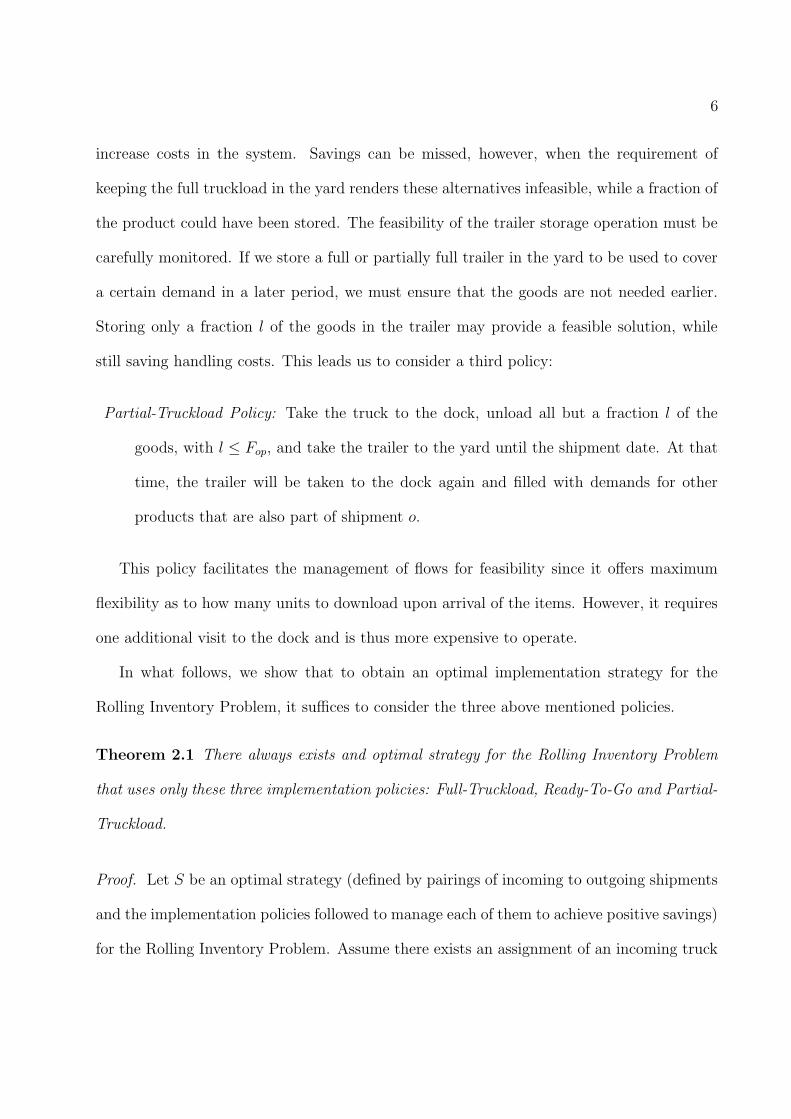
Partial-Truckload Policy: Take the truck to the dock, unload all but a fraction l of the

goods, with l ≤ Fop, and take the trailer to the yard until the shipment date. At that

time, the trailer will be taken to the dock again and filled with demands for other

products that are also part of shipment o.

This policy facilitates the management of flows for feasibility since it offers maximum

flexibility as to how many units to download upon arrival of the items. However, it requires

one additional visit to the dock and is thus more expensive to operate.

In what follows, we show that to obtain an optimal implementation strategy for the

Rolling Inventory Problem, it suffices to consider the three above mentioned policies.

Theorem 2.1 There always exists and optimal strategy for the Rolling Inventory Problem

that uses only these three implementation policies: Full-Truckload, Ready-To-Go and Partial-

Truckload.

Proof. Let S be an optimal strategy (defined by pairings of incoming to outgoing shipments

and the implementation policies followed to manage each of them to achieve positive savings)

for the Rolling Inventory Problem. Assume there exists an assignment of an incoming truck

7

of product p at time period t to an outgoing shipment o at time period s ≥ t using an

implementation policy different from the three above. If either the Full-Truckload or the

Ready-To-Go policies are feasible (i.e. there is enough materials to satisfy the demands in

the intermediate outgoing shipments between s and t when following these policies) within

strategy S, then we would increase savings by switching to these policies. This contradicts

the optimality of the initial solution S. Thus, s > t and it must not be feasible to leave

the full trailer in the yard or to load the entire mix of products upon arrival at t and store

the goods in the trailer up until time s. Let z > 0 be the amount of product p t hat is

never unloaded into the warehouse. It must be a positive amount in order for the pairing

to achieve positive savings, ch min{z, Fop}, and be part of an optimal strategy. Since the

quantity z is never downloaded in the feasible strategy S, the Partial-Truck load policy with

l = min{z, Fop} is also feasible and achieves the same savings in handling. All that remains

to show is that transportation costs are no higher when using this policy. The Partial-

Truckload policy requires (1) the arriving truck to stop at the dock at time t, (2) the trailer

to be taken to the yard, (3) the trailer to be picked up from the yard and taken back to

the dock at time s, and (4) final shipment from the dock. Observe that any feasible policy

will require two visits to the dock (as the Partial-Truckload policy) and/or two visits to the

yard. Any policy that requires two visits to the dock, will lead to savings no higher than the

Partial-Truckload policy and thus we can simply change the implementation of that pairing

to the Partial-Truckload policy. If the policy requires two visits to the yard, the minimum

possible transportation costs associated will involve: (1) taking the trailer to the yard, (2)

picking the trailer up from the yard to the dock, (3) taking the trailer back to the yard, and

(4) picking the trailer up from the yard. These costs are no smaller than those associated

with the Partial-Truckload policy. Thus, we can always construct a solution with equal or

8

better cost that only uses the three described implementation policies.

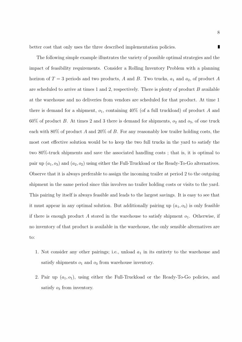
The following simple example illustrates the variety of possible optimal strategies and the

impact of feasibility requirements. Consider a Rolling Inventory Problem with a planning

horizon of T = 3 periods and two products, A and B. Two trucks, a1 and a2, of product A

are scheduled to arrive at times 1 and 2, respectively. There is plenty of product B available

at the warehouse and no deliveries from vendors are scheduled for that product. At time 1

there is demand for a shipment, o1, containing 40% (of a full truckload) of product A and

60% of product B. At times 2 and 3 there is demand for shipments, o2 and o3, of one truck

each with 80% of product A and 20% of B. For any reasonably low trailer holding costs, the

most cost effective solution would be to keep the two full trucks in the yard to satisfy the

two 80%-truck shipments and save the associated handling costs ; that is, it is optimal to

pair up (a1, o3) and (a2, o2) using either the Full-Truckload or the Ready-To-Go alternatives.

Observe that it is always preferable to assign the incoming trailer at period 2 to the outgoing

shipment in the same period since this involves no trailer holding costs or visits to the yard.

This pairing by itself is always feasible and leads to the largest savings. It is easy to see that

it must appear in any optimal solution. But additionally pairing up (a1, o3) is only feasible

if there is enough product A stored in the warehouse to satisfy shipment o1. Otherwise, if

no inventory of that product is available in the warehouse, the only sensible alternatives are

to:

1. Not consider any other pairings; i.e., unload a1 in its entirety to the warehouse and

satisfy shipments o1 and o3 from warehouse inventory.

2. Pair up (a1, o1), using either the Full-Truckload or the Ready-To-Go policies, and

satisfy o3 from inventory.

9

3. Pair up (a1, o3) using policy 2 with l = 0.6 and satisfying shipment o1 with the material

downloaded to the warehouse.

Which of these strategies to use depends on the particular parameters of the problem.

Finally, observe that the Partial-Truckload policy may not be cost-efficient when there

are large fixed costs in transportation and dock operations. The Ready-To-Go policy, on

the other hand, reduces the flexibility to accommodate last-minute changes in orders and

may end up increasing costs if customers occasionally modify their orders as the delivery

date approaches. As a result, in practice, it may be attractive to consider the Full-Truckload

policy in isolation, as the only alternative, to simplify the management of materials through

the warehouse complex. Section 2 addresses the Rolling Inventory Problem in that case and

Section 3 considers the general case in which the optimal strategy can be any mixture of the

three policies: Full-Truckload, Partial-Truckload and Ready-To-Go .

3 Full-Truckload Case

In this section we consider the Rolling Inventory Problem under the assumption that trailers

are only stored in the yard full, directly upon arrival; i.e., under the Full-Truckload policy.

We consider P products indexed by p, T periods of time indexed by t and N outgoing trucks

indexed by o. Each outgoing truck o is made up of a certain mix of products. We consider

a full truckload to be the unit of measurement for all products. We define the following

parameters:

To = departure time of outgoing shipment o

Apt = number of arriving trucks of product p at time t.

Fop = fraction of a truckload of product p in outgoing shipment o.

10

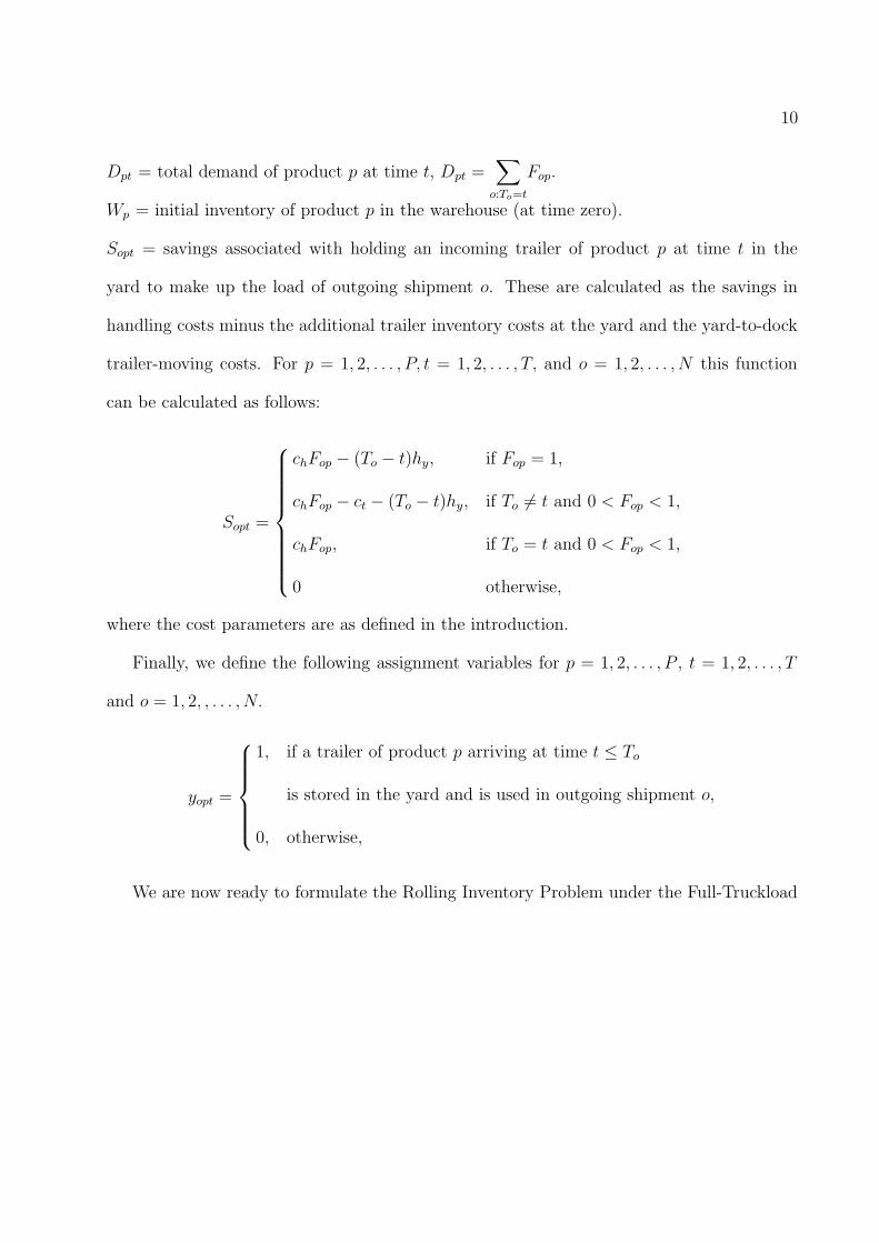
Dpt = total demand of product p at time t, Dpt =∑

o:To=t

Fop.

Wp = initial inventory of product p in the warehouse (at time zero).

Sopt = savings associated with holding an incoming trailer of product p at time t in the

yard to make up the load of outgoing shipment o. These are calculated as the savings in

handling costs minus the additional trailer inventory costs at the yard and the yard-to-dock

trailer-moving costs. For p = 1, 2, . . . , P, t = 1, 2, . . . , T, and o = 1, 2, . . . , N this function

can be calculated as follows:

Sopt =

chFop − (To − t)hy, if Fop = 1,

chFop − ct − (To − t)hy, if To 6= t and 0 < Fop < 1,

chFop, if To = t and 0 < Fop < 1,

0 otherwise,

where the cost parameters are as defined in the introduction.

Finally, we define the following assignment variables for p = 1, 2, . . . , P , t = 1, 2, . . . , T

and o = 1, 2, , . . . , N.

yopt =

1, if a trailer of product p arriving at time t ≤ To

is stored in the yard and is used in outgoing shipment o,

0, otherwise,

We are now ready to formulate the Rolling Inventory Problem under the Full-Truckload

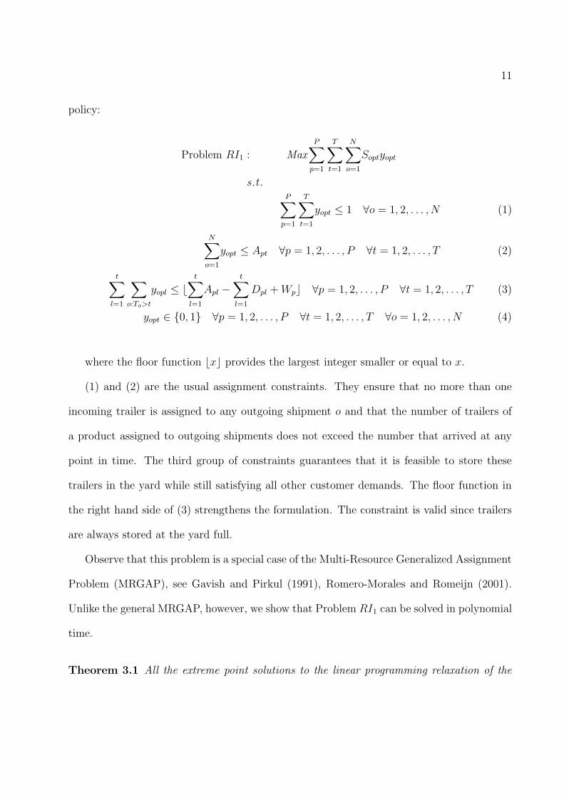
11

policy:

Problem RI1 : MaxP

∑

p=1

T∑

t=1

N∑

o=1

Soptyopt

s .t .P

∑

p=1

T∑

t=1

yopt ≤ 1 ∀o = 1, 2, . . . , N (1)

N∑

o=1

yopt ≤ Apt ∀p = 1, 2, . . . , P ∀t = 1, 2, . . . , T (2)

t∑

l=1

∑

o:To>t

yopl ≤ b

t∑

l=1

Apl −

t∑

l=1

Dpl + Wpc ∀p = 1, 2, . . . , P ∀t = 1, 2, . . . , T (3)

yopt ∈ {0, 1} ∀p = 1, 2, . . . , P ∀t = 1, 2, . . . , T ∀o = 1, 2, . . . , N (4)

where the floor function bxc provides the largest integer smaller or equal to x.

(1) and (2) are the usual assignment constraints. They ensure that no more than one

incoming trailer is assigned to any outgoing shipment o and that the number of trailers of

a product assigned to outgoing shipments does not exceed the number that arrived at any

point in time. The third group of constraints guarantees that it is feasible to store these

trailers in the yard while still satisfying all other customer demands. The floor function in

the right hand side of (3) strengthens the formulation. The constraint is valid since trailers

are always stored at the yard full.

Observe that this problem is a special case of the Multi-Resource Generalized Assignment

Problem (MRGAP), see Gavish and Pirkul (1991), Romero-Morales and Romeijn (2001).

Unlike the general MRGAP, however, we show that Problem RI1 can be solved in polynomial

time.

Theorem 3.1 All the extreme point solutions to the linear programming relaxation of the

12

Rolling Inventory Problem under the Full-Truckload policy, RI1, are integer.

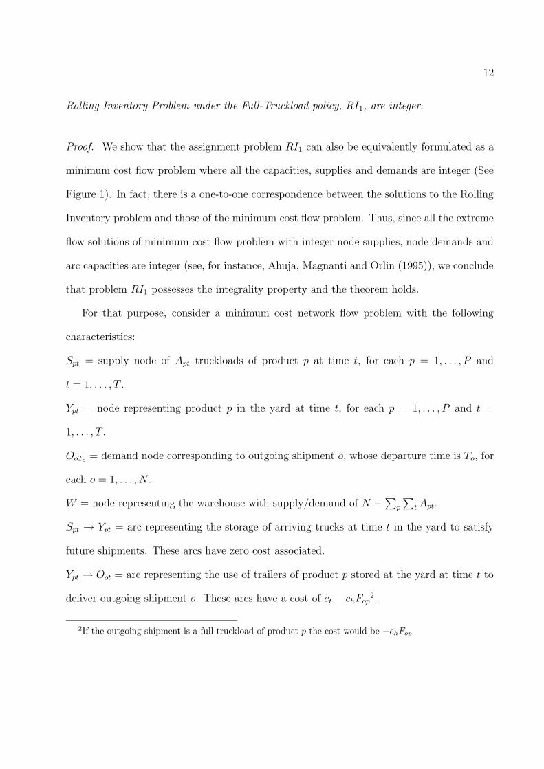
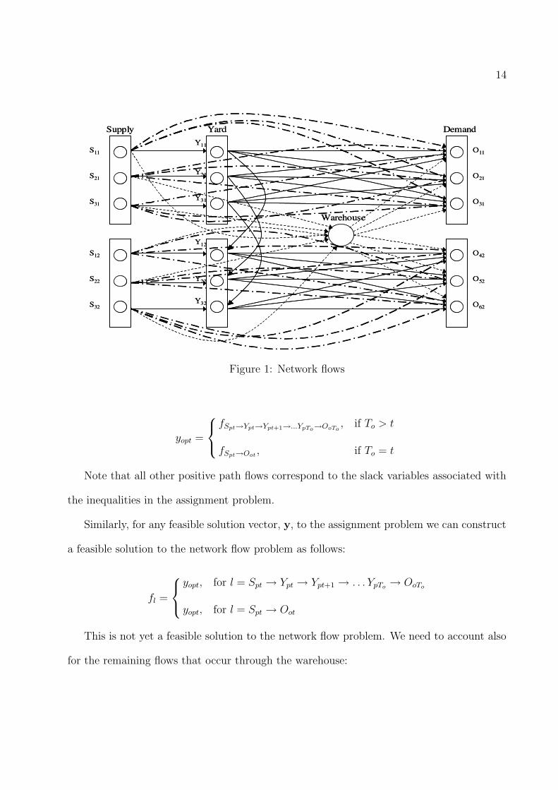
Proof. We show that the assignment problem RI1 can also be equivalently formulated as a

minimum cost flow problem where all the capacities, supplies and demands are integer (See

Figure 1). In fact, there is a one-to-one correspondence between the solutions to the Rolling

Inventory problem and those of the minimum cost flow problem. Thus, since all the extreme

flow solutions of minimum cost flow problem with integer node supplies, node demands and

arc capacities are integer (see, for instance, Ahuja, Magnanti and Orlin (1995)), we conclude

that problem RI1 possesses the integrality property and the theorem holds.

For that purpose, consider a minimum cost network flow problem with the following

characteristics:

Spt = supply node of Apt truckloads of product p at time t, for each p = 1, . . . , P and

t = 1, . . . , T .

Ypt = node representing product p in the yard at time t, for each p = 1, . . . , P and t =

1, . . . , T .

OoTo= demand node corresponding to outgoing shipment o, whose departure time is To, for

each o = 1, . . . , N .

W = node representing the warehouse with supply/demand of N −∑

p

∑

t Apt.

Spt → Ypt = arc representing the storage of arriving trucks at time t in the yard to satisfy

future shipments. These arcs have zero cost associated.

Ypt → Oot = arc representing the use of trailers of product p stored at the yard at time t to

deliver outgoing shipment o. These arcs have a cost of ct − chFop2.

2If the outgoing shipment is a full truckload of product p the cost would be −chFop

13

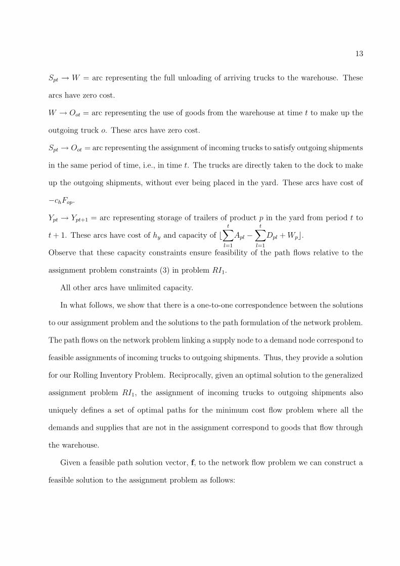
Spt → W = arc representing the full unloading of arriving trucks to the warehouse. These

arcs have zero cost.

W → Oot = arc representing the use of goods from the warehouse at time t to make up the

outgoing truck o. These arcs have zero cost.

Spt → Oot = arc representing the assignment of incoming trucks to satisfy outgoing shipments

in the same period of time, i.e., in time t. The trucks are directly taken to the dock to make

up the outgoing shipments, without ever being placed in the yard. These arcs have cost of

−chFop.

Ypt → Ypt+1 = arc representing storage of trailers of product p in the yard from period t to

t + 1. These arcs have cost of hy and capacity of bt

∑

l=1

Apl −

t∑

l=1

Dpl + Wpc.

Observe that these capacity constraints ensure feasibility of the path flows relative to the

assignment problem constraints (3) in problem RI1.

All other arcs have unlimited capacity.

In what follows, we show that there is a one-to-one correspondence between the solutions

to our assignment problem and the solutions to the path formulation of the network problem.

The path flows on the network problem linking a supply node to a demand node correspond to

feasible assignments of incoming trucks to outgoing shipments. Thus, they provide a solution

for our Rolling Inventory Problem. Reciprocally, given an optimal solution to the generalized

assignment problem RI1, the assignment of incoming trucks to outgoing shipments also

uniquely defines a set of optimal paths for the minimum cost flow problem where all the

demands and supplies that are not in the assignment correspond to goods that flow through

the warehouse.

Given a feasible path solution vector, f, to the network flow problem we can construct a

feasible solution to the assignment problem as follows:

14

Supply Yard

S11

Demand

S21

S31

S12

S22

S32

Y11

Y21

Y31

Y12

Y22

Y32

Warehouse

O11

O21

O31

O42

O52

O62

Supply Yard

S11

Demand

S21

S31

S12

S22

S32

Y11

Y21

Y31

Y12

Y22

Y32

Warehouse

O11

O21

O31

O42

O52

O62

Figure 1: Network flows

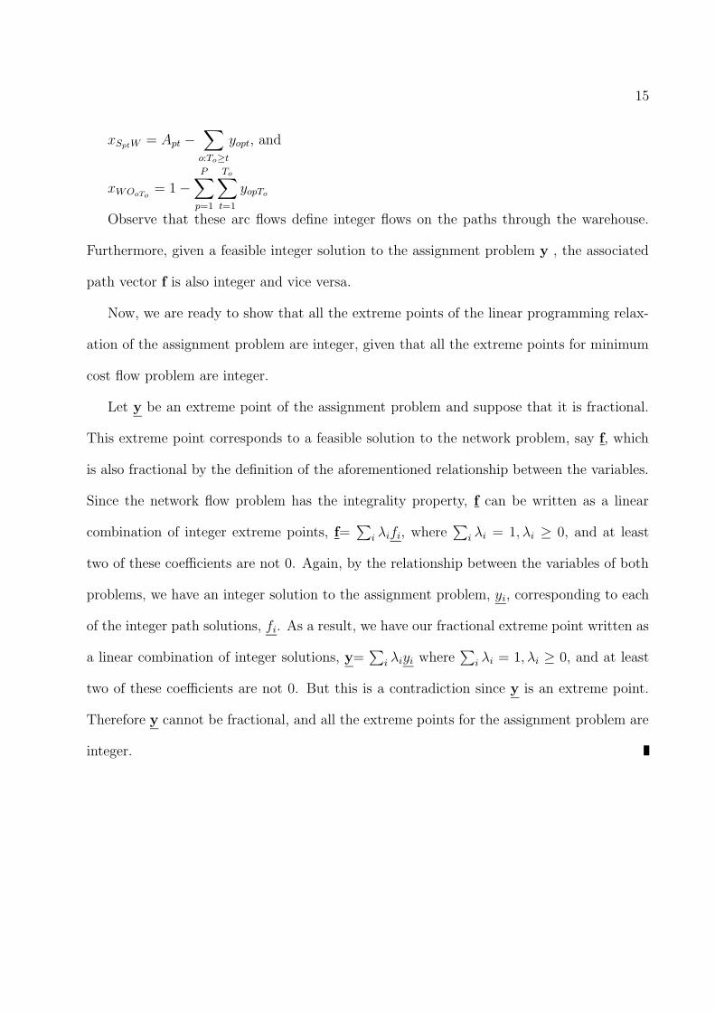
yopt =

fSpt→Ypt→Ypt+1→...YpTo→OoTo, if To > t

fSpt→Oot, if To = t

Note that all other positive path flows correspond to the slack variables associated with

the inequalities in the assignment problem.

Similarly, for any feasible solution vector, y, to the assignment problem we can construct

a feasible solution to the network flow problem as follows:

fl =

yopt, for l = Spt → Ypt → Ypt+1 → . . . YpTo→ OoTo

yopt, for l = Spt → Oot

This is not yet a feasible solution to the network flow problem. We need to account also

for the remaining flows that occur through the warehouse:

15

xSptW = Apt −∑

o:To≥t

yopt, and

xWOoTo= 1 −

P∑

p=1

To∑

t=1

yopTo

Observe that these arc flows define integer flows on the paths through the warehouse.

Furthermore, given a feasible integer solution to the assignment problem y , the associated

path vector f is also integer and vice versa.

Now, we are ready to show that all the extreme points of the linear programming relax-

ation of the assignment problem are integer, given that all the extreme points for minimum

cost flow problem are integer.

Let y be an extreme point of the assignment problem and suppose that it is fractional.

This extreme point corresponds to a feasible solution to the network problem, say f, which

is also fractional by the definition of the aforementioned relationship between the variables.

Since the network flow problem has the integrality property, f can be written as a linear

combination of integer extreme points, f=∑

i λifi, where∑

i λi = 1, λi ≥ 0, and at least

two of these coefficients are not 0. Again, by the relationship between the variables of both

problems, we have an integer solution to the assignment problem, yi, corresponding to each

of the integer path solutions, fi. As a result, we have our fractional extreme point written as

a linear combination of integer solutions, y=∑

i λiyi where∑

i λi = 1, λi ≥ 0, and at least

two of these coefficients are not 0. But this is a contradiction since y is an extreme point.

Therefore y cannot be fractional, and all the extreme points for the assignment problem are

integer.

16

4 General Case

In this section we formulate the problem in the general case where the optimal strategy

uses any of the three implementation policies – Full-Truckload, Ready-To-Go and Partial-

Truckload. Recall that it suffices to consider these 3 alternatives to generate optimal solutions

to the Rolling Inventory problem (RI).

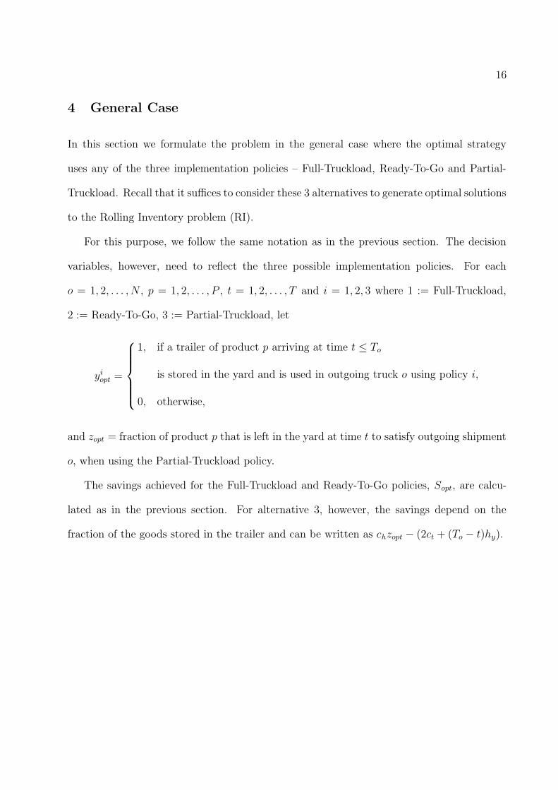
For this purpose, we follow the same notation as in the previous section. The decision

variables, however, need to reflect the three possible implementation policies. For each

o = 1, 2, . . . , N , p = 1, 2, . . . , P , t = 1, 2, . . . , T and i = 1, 2, 3 where 1 := Full-Truckload,

2 := Ready-To-Go, 3 := Partial-Truckload, let

yiopt =

1, if a trailer of product p arriving at time t ≤ To

is stored in the yard and is used in outgoing truck o using policy i,

0, otherwise,

and zopt = fraction of product p that is left in the yard at time t to satisfy outgoing shipment

o, when using the Partial-Truckload policy.

The savings achieved for the Full-Truckload and Ready-To-Go policies, Sopt, are calcu-

lated as in the previous section. For alternative 3, however, the savings depend on the

fraction of the goods stored in the trailer and can be written as chzopt − (2ct + (To − t)hy).

17

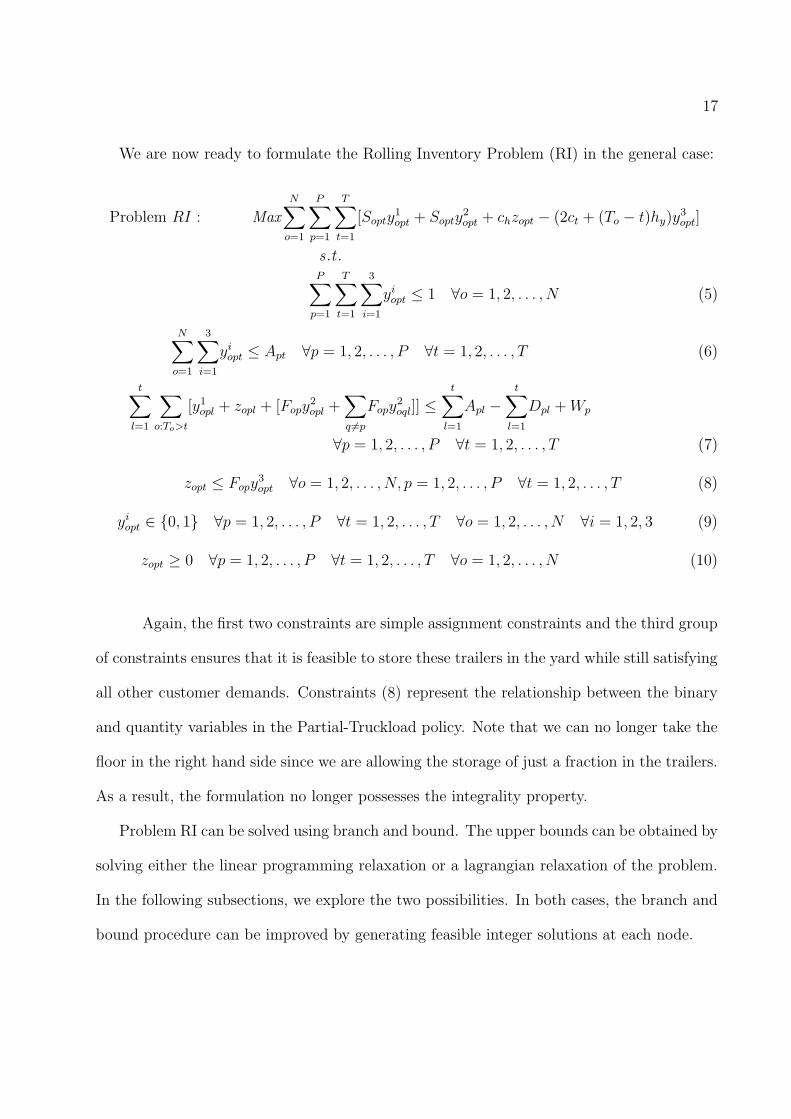
We are now ready to formulate the Rolling Inventory Problem (RI) in the general case:

Problem RI : MaxN

∑

o=1

P∑

p=1

T∑

t=1

[Sopty1

opt + Sopty2

opt + chzopt − (2ct + (To − t)hy)y3

opt]

s .t .P

∑

p=1

T∑

t=1

3∑

i=1

yiopt ≤ 1 ∀o = 1, 2, . . . , N (5)

N∑

o=1

3∑

i=1

yiopt ≤ Apt ∀p = 1, 2, . . . , P ∀t = 1, 2, . . . , T (6)

t∑

l=1

∑

o:To>t

[y1

opl + zopl + [Fopy2

opl +∑

q 6=p

Fopy2

oql]] ≤t

∑

l=1

Apl −t

∑

l=1

Dpl + Wp

∀p = 1, 2, . . . , P ∀t = 1, 2, . . . , T (7)

zopt ≤ Fopy3

opt ∀o = 1, 2, . . . , N, p = 1, 2, . . . , P ∀t = 1, 2, . . . , T (8)

yiopt ∈ {0, 1} ∀p = 1, 2, . . . , P ∀t = 1, 2, . . . , T ∀o = 1, 2, . . . , N ∀i = 1, 2, 3 (9)

zopt ≥ 0 ∀p = 1, 2, . . . , P ∀t = 1, 2, . . . , T ∀o = 1, 2, . . . , N (10)

Again, the first two constraints are simple assignment constraints and the third group

of constraints ensures that it is feasible to store these trailers in the yard while still satisfying

all other customer demands. Constraints (8) represent the relationship between the binary

and quantity variables in the Partial-Truckload policy. Note that we can no longer take the

floor in the right hand side since we are allowing the storage of just a fraction in the trailers.

As a result, the formulation no longer possesses the integrality property.

Problem RI can be solved using branch and bound. The upper bounds can be obtained by

solving either the linear programming relaxation or a lagrangian relaxation of the problem.

In the following subsections, we explore the two possibilities. In both cases, the branch and

bound procedure can be improved by generating feasible integer solutions at each node.

18

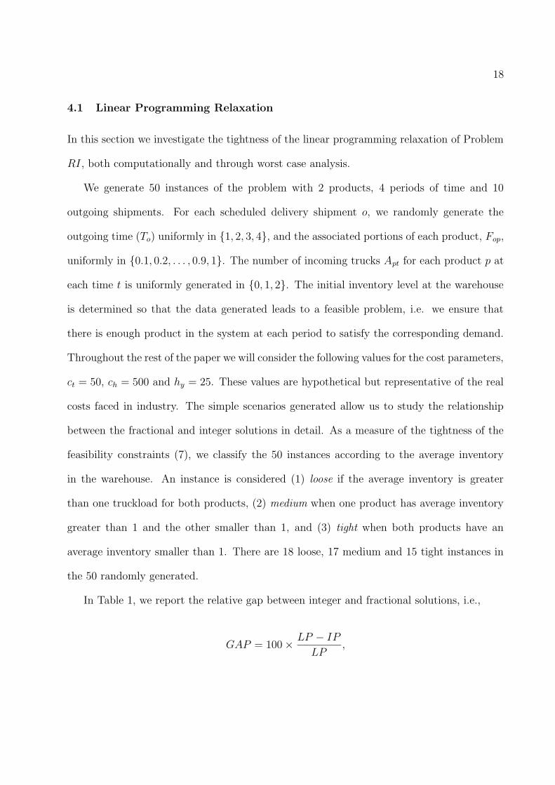
4.1 Linear Programming Relaxation

In this section we investigate the tightness of the linear programming relaxation of Problem

RI, both computationally and through worst case analysis.

We generate 50 instances of the problem with 2 products, 4 periods of time and 10

outgoing shipments. For each scheduled delivery shipment o, we randomly generate the

outgoing time (To) uniformly in {1, 2, 3, 4}, and the associated portions of each product, Fop,

uniformly in {0.1, 0.2, . . . , 0.9, 1}. The number of incoming trucks Apt for each product p at

each time t is uniformly generated in {0, 1, 2}. The initial inventory level at the warehouse

is determined so that the data generated leads to a feasible problem, i.e. we ensure that

there is enough product in the system at each period to satisfy the corresponding demand.

Throughout the rest of the paper we will consider the following values for the cost parameters,

ct = 50, ch = 500 and hy = 25. These values are hypothetical but representative of the real

costs faced in industry. The simple scenarios generated allow us to study the relationship

between the fractional and integer solutions in detail. As a measure of the tightness of the

feasibility constraints (7), we classify the 50 instances according to the average inventory

in the warehouse. An instance is considered (1) loose if the average inventory is greater

than one truckload for both products, (2) medium when one product has average inventory

greater than 1 and the other smaller than 1, and (3) tight when both products have an

average inventory smaller than 1. There are 18 loose, 17 medium and 15 tight instances in

the 50 randomly generated.

In Table 1, we report the relative gap between integer and fractional solutions, i.e.,

GAP = 100 ×LP − IP

LP,

19

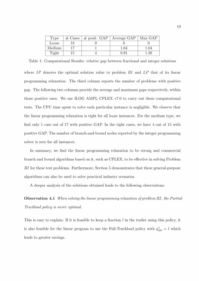
Type # Cases # posit. GAP Average GAP Max GAPLoose 18 0 0 0

Medium 17 1 1.04 1.04Tight 15 4 0.91 1.38

Table 1: Computational Results: relative gap between fractional and integer solutions

where IP denotes the optimal solution value to problem RI and LP that of its linear

programming relaxation. The third column reports the number of problems with positive

gap. The following two columns provide the average and maximum gaps respectively, within

those positive ones. We use ILOG AMPL CPLEX v7.0 to carry out these computational

tests. The CPU time spent to solve each particular instance is negligible. We observe that

the linear programming relaxation is tight for all loose instances. For the medium type, we

find only 1 case out of 17 with positive GAP. In the tight cases, we have 4 out of 15 with

positive GAP. The number of branch-and-bound nodes reported by the integer programming

solver is zero for all instances.

In summary, we find the linear programming relaxation to be strong and commercial

branch and bound algorithms based on it, such as CPLEX, to be effective in solving Problem

RI for these test problems. Furthermore, Section 5 demonstrates that these general-purpose

algorithms can also be used to solve practical industry scenarios.

A deeper analysis of the solutions obtained leads to the following observations.

Observation 4.1 When solving the linear programming relaxation of problem RI, the Partial-

Truckload policy is never optimal.

This is easy to explain: If it is feasible to keep a fraction l in the trailer using this policy, it

is also feasible for the linear program to use the Full-Truckload policy with y1opt = l which

leads to greater savings.

20

Observation 4.2 The linear programming relaxation for the general case may generate a

fractional solution even if an integer solution with the same value exists.

We have observed numerous cases where the linear program splits the assignment of one

incoming truck to an outgoing shipment between the Full-Truckload and the Ready-To-Go

policies, even though it is feasible to use just one of the alternatives (but not feasible to use

both since otherwise it would not be an extreme point solution). Since the savings function

is the same for both policies, both solutions lead to the same objective value. To avoid this

problem, one could think of increasing the savings associated with one of the alternatives,

say policy 1 (Full-Truckload), by a small amount, ε. Then, if that alternative is feasible

the linear program would not split between the two and thus generate an integral solution.

Unfortunately, this is not always the case. If policy 1 is not feasible, this additional savings

drive the linear program to use it for as large a portion of the assignment as possible, forcing

the solution to be fractional. Thus, this approach would not necessarily help in increasing

the number of integer variables in the solution to the linear program.

B A

.1(A)/.9(B).9(A)/.1(B)

1 21GAP = 100 %

Warehouse.9 (A)

20

Arriving Trucks

Outgoing Trucks1 2

2

B A

.1(A)/.9(B).9(A)/.1(B)

1 21GAP = 100 %

Warehouse.9 (A)

20

Arriving Trucks

Outgoing Trucks1 2

2

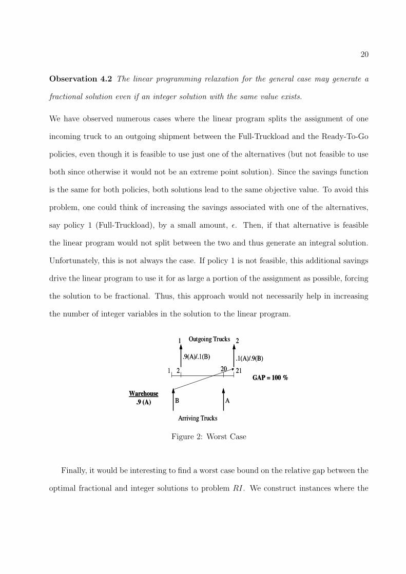
Figure 2: Worst Case

Finally, it would be interesting to find a worst case bound on the relative gap between the

optimal fractional and integer solutions to problem RI. We construct instances where the

21

linear program finds a positive solution while no positive savings can be achieved in reality.

Thus, the relative gap can be as large as 100%.

Observation 4.3 The relative gap between integer and fractional solutions can be as large

as 100%.

The example in Figure 2 illustrates this situation. When the linear programming relax-

ation is solved, the incoming truck of product B arriving at time 1 is assigned to the second

outgoing shipment with y12B1 = 0.9. Note that we cannot store the full truck of product

B since we need 10% of the product to satisfy the first outgoing shipment. When solving

the integer program, however, neither the Full-Truckload nor the Ready-To-Go policies are

feasible. Furthermore, the Partial-Truckload Policy does not yield any positive savings. The

optimal savings in this case are thus zero. Then, the GAP would be 100% as we mentioned

above.

It is easy to construct a feasible integer solution from a fractional one as follows. Order

the fractional assignment variables using some priority rule; e.g., according to their fractional

values or the timing of the shipments. Considered in that order, set each variable to 1 unless

a constraint is violated, in which case the variable is set to 0.

4.2 Lagrangian Relaxation

Lagrangian relaxation techniques are commonly used to solve integer programming problems

and have been proposed for the MRGAP (Gavish and Pirkul (1991)). In this section, we

investigate the application of such techniques to Problem RI.

Observe that relaxing constraints (5) results in a Lagrangian problem that decomposes

over the products, p, but is not much easier to solve than the original one. Similarly, relaxing

22

constraints (6) is not appealing, since all the variables would continue to be linked by the

remaining constraints. Thus, we focus on the relaxation of constraint set (7), which leads to

the following lagrangian problem.

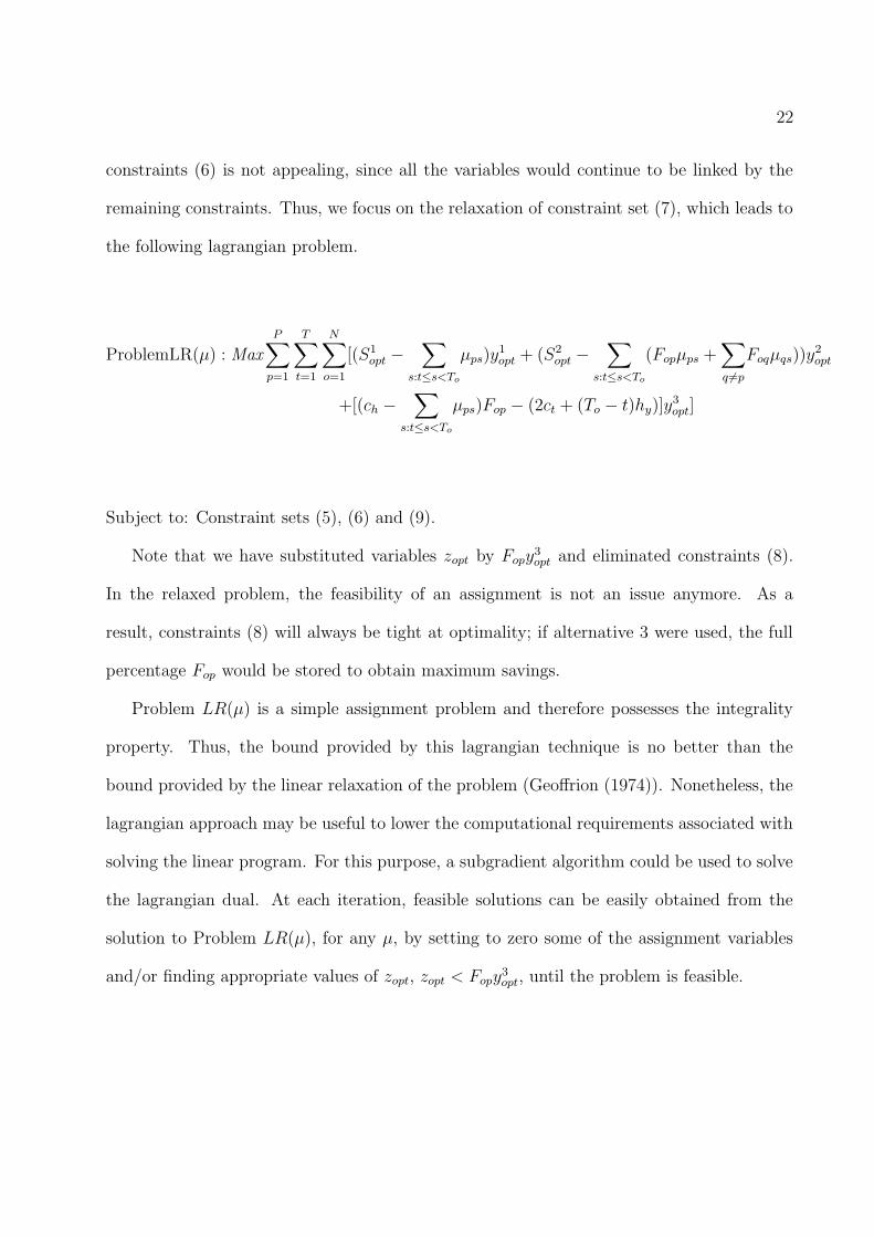
ProblemLR(µ) : MaxP

∑

p=1

T∑

t=1

N∑

o=1

[(S1

opt −∑

s:t≤s<To

µps)y1

opt + (S2

opt −∑

s:t≤s<To

(Fopµps +∑

q 6=p

Foqµqs))y2

opt

+[(ch −∑

s:t≤s<To

µps)Fop − (2ct + (To − t)hy)]y3

opt]

Subject to: Constraint sets (5), (6) and (9).

Note that we have substituted variables zopt by Fopy3opt and eliminated constraints (8).

In the relaxed problem, the feasibility of an assignment is not an issue anymore. As a

result, constraints (8) will always be tight at optimality; if alternative 3 were used, the full

percentage Fop would be stored to obtain maximum savings.

Problem LR(µ) is a simple assignment problem and therefore possesses the integrality

property. Thus, the bound provided by this lagrangian technique is no better than the

bound provided by the linear relaxation of the problem (Geoffrion (1974)). Nonetheless, the

lagrangian approach may be useful to lower the computational requirements associated with

solving the linear program. For this purpose, a subgradient algorithm could be used to solve

the lagrangian dual. At each iteration, feasible solutions can be easily obtained from the

solution to Problem LR(µ), for any µ, by setting to zero some of the assignment variables

and/or finding appropriate values of zopt, zopt < Fopy3opt, until the problem is feasible.

23

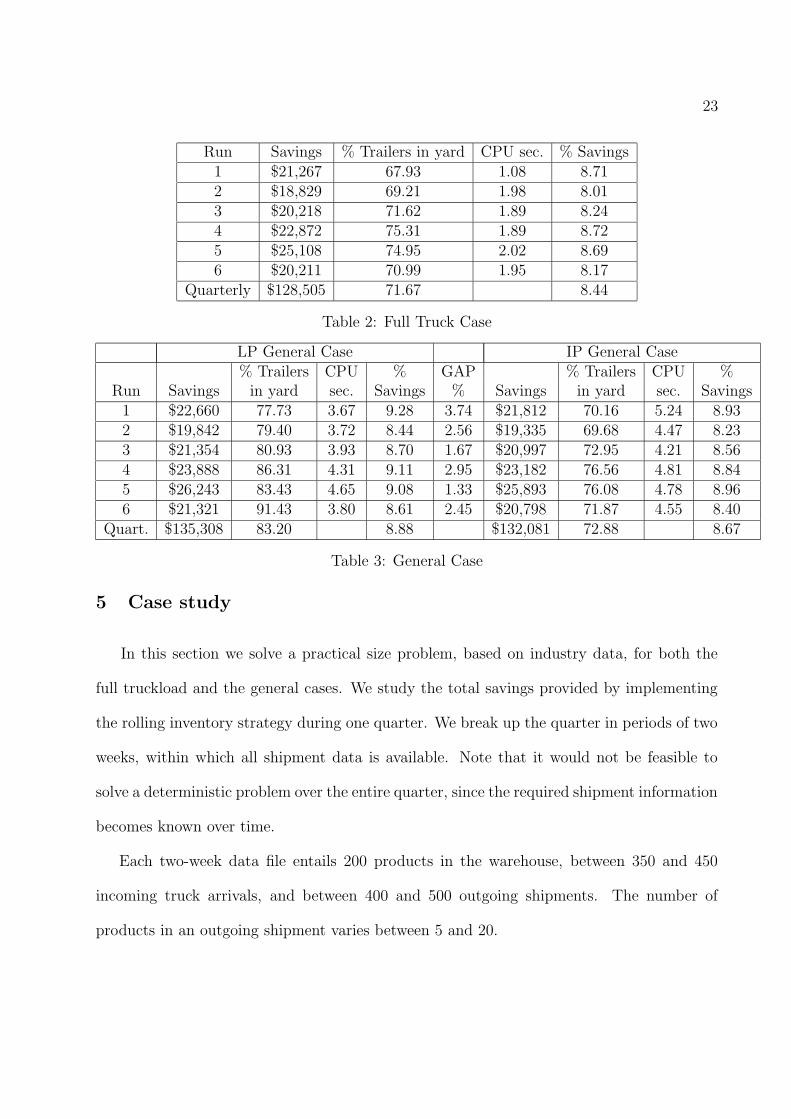
Run Savings % Trailers in yard CPU sec. % Savings1 $21,267 67.93 1.08 8.712 $18,829 69.21 1.98 8.013 $20,218 71.62 1.89 8.244 $22,872 75.31 1.89 8.725 $25,108 74.95 2.02 8.696 $20,211 70.99 1.95 8.17

Quarterly $128,505 71.67 8.44

Table 2: Full Truck Case

LP General Case IP General Case% Trailers CPU % GAP % Trailers CPU %

Run Savings in yard sec. Savings % Savings in yard sec. Savings1 $22,660 77.73 3.67 9.28 3.74 $21,812 70.16 5.24 8.932 $19,842 79.40 3.72 8.44 2.56 $19,335 69.68 4.47 8.233 $21,354 80.93 3.93 8.70 1.67 $20,997 72.95 4.21 8.564 $23,888 86.31 4.31 9.11 2.95 $23,182 76.56 4.81 8.845 $26,243 83.43 4.65 9.08 1.33 $25,893 76.08 4.78 8.966 $21,321 91.43 3.80 8.61 2.45 $20,798 71.87 4.55 8.40

Quart. $135,308 83.20 8.88 $132,081 72.88 8.67

Table 3: General Case

5 Case study

In this section we solve a practical size problem, based on industry data, for both the

full truckload and the general cases. We study the total savings provided by implementing

the rolling inventory strategy during one quarter. We break up the quarter in periods of two

weeks, within which all shipment data is available. Note that it would not be feasible to

solve a deterministic problem over the entire quarter, since the required shipment information

becomes known over time.

Each two-week data file entails 200 products in the warehouse, between 350 and 450

incoming truck arrivals, and between 400 and 500 outgoing shipments. The number of

products in an outgoing shipment varies between 5 and 20.

24

We use ILOG CPLEX v6.5 to solve the problem. The results are given in Tables 2 and 3,

for the Full-Truckload and General cases, respectively. The tables include the total savings

and the percentage of trailers stored in the yard when implementing the rolling inventory

strategy, the CPU times used in solving the problem, and the relative savings as compared

to unloading all arriving product to the warehouse. For the general case, we also report

information on the linear programming relaxation and the GAP between the fractional and

integer solutions, where again GAP is defined as GAP = 100 × LP−IPLP

.

Summarizing the results obtained, the rolling inventory approach leads to total savings

of over $128,000 dollars under the simplest implementation policy, Full-Truckload, which

allows only full arriving truckloads in the yard. This represents savings of 8% in quarterly

warehouse operations. Surprisingly, no significant additional savings (only a 0.23% increase)

are gained by jointly considering the three policies to ensure an overall optimal solution.

Using the Full-Truckload policy in isolation is indeed a very attractive alternative in order

to keep the management of the operation simple while reaping most of the benefits of the

rolling inventory strategy. Finally, we observe that, for the instances studied, it is possible

to solve the general problem optimally without a significant increase in computation time.

This is due to the tightness of the linear programming relaxation.

6 Conclusions

In this paper we present a new strategy in warehouse management, Rolling Inventory, that

allows for the storage of products in the trailers where they were shipped. This saves handling

costs and storage space at the expense of some extra trailer movements and the opportunity

costs of using the trailers. Additional advantages of the rolling inventory strategy are the

25

reduction of product damage, handling complexity and storage requirements in the ware-

house. We introduce three different implementation policies: Full-Truckload, Ready-To-Go

and Partial-Truckload. We show that it suffices to consider these three policies in order to

make optimal use of the rolling inventory strategy.

Our computational study shows that rolling inventory leads to considerable savings,

around 8%, for real size problems. Moreover, a simple policy that only allows for trucks

to be stored in the yard full upon arrival, namely the Full Truckload policy, provides savings

that are fairly close to optimal (leading to only a 0.23% decrease in savings). This policy

facilitates the implementation of the rolling inventory strategy from both managerial and

computational standpoints, which makes it very attractive in practice. Under such policy,

we show that the problem of determining which incoming trucks to store, their contents

and the length of their stay, has the integrality property and can thus be solved as a simple

linear program. In addition, we would like to point out that this policy has a much higher

potential for acceptance in the field. In the warehousing operations that we are familiar

with, managers have a very strong preference towards moving full trucks.

We have managed to solve real instances of the problem optimally, i.e. for the general

case, using a commercial integer programming solver. The optimal solution was generated

in just a few seconds due to the tightness of the linear relaxation of our problem formulation.

However, it would be interesting to study heuristics or exact algorithms that can provide

the optimal integer solution in polynomial time. Finally, since the data on scheduled supply

arrivals and customer orders becomes known over time, the stochastic version of the problem

will have a wider range of application and needs to be studied.

Acknowledgements: We would like to thank Bruce Gamble (Schneider Logistics) and

Matt Littleton (Kimberly Clark) for introducing us to this problem and providing us with

26

invaluable industry insight.

7 References

Ahuja, R.K., Magnanti, T.L. and Orlin, J.B. (1993) Network Flows. Theory, Algorithms

and applications. Prentice Hall.

Bramel, J. and Simchi-Levi D. (1997) The Logic of Logistics: Theory, Algorithms, and Ap-

plications for Logistics Management. Springer Series in Operations Research, Springer-

Verlag, New York.

Blocq, R.,Romero Morales, D., Romeijn, H., and Timmer, G. (2000) The multi-resource gen-

eralized assignment problem with and application to the distribution of gasoline prod-

ucts. Working Paper, Department of Decision and Information Sciences, Rotterdam

School of Management, The Netherlands.

Campbell, J. and Langevin, A. (1995) The snow disposal assignment problem. Journal of

the Operational Research Society, 46:919-929.

Cattrysse, D. and Van Wassenhove, L. (1992) A survey of algorithms for the generalized

assignment problem. European Journal of Operational Research, 60:260-272.

Comier, G. and Gunn, E.A. (1992) A review of warehouse models. European Journal of

Operational Research, 58:3-13.

Croxton K. L., B. Gendron and T. L. Magnanti (2003) Models and Methods for Merge-In-

Transit Operations. To appear in Transportation Science.

Fisher, M. and Jaikumar, R. (1981) A generalized assignment heuristic for vehicle routing.

Networks, 11:109-124.

Gavish, B. and Pirkul, H. (1991) Algorithms for the multi-resource generalized assignment

27

problem. Management Science, 37(6):695-713.

Geoffrion, A. M. (1974) Lagrangian Relaxation and its Uses in Integer Programming. Math

Programming Study 2, 82–114.

Osman, I. (1995) Heuristics for the generalized assignment problem: simulated annealing

and tabu search approaches. OR Spektrum, 17:211-225.

Romeijn, H. and Romero Morales, D. (2000) A class of greedy algorithms for the generalized

assignment problem. Discrete Applied Mathematics, 103:209-235.

Romero Morales, D. and Romeijn, H.E. The generalized assignment problem and extensions.

Forthcoming in: Handbook of Combinatorial Optimization, supplement volume B (D.Z.

Du and P.M. Pardalos, eds.), Kluwer Academic Publishers, Dordrecht, The Netherlands.

Ross, G. and Soland, R. (1975) A branch and bound algorithm for the generalized assignment

problem. Mathematical Programming, 8:91-103.

Ross, G. and Soland, R. (1977) Modelling facility location problems as generalized assignment

problems. Management Science, 24(3):345-357.