Guaranteeing Benefits in Generational Pension Plans

Xiaohong HuangSchool of Management and Governance, University of Twente,

Drienerlolaan 5, 7522 NB Enschede, the Netherlands.E-mail: x.huang@utwente.nl

Ronald MahieuDepartment of Econometrics and Operations Research,Tilburg University,

Warandelaan 2, 5000 LE Tilburg, the Netherlands.Tel: 0031 53 4893458, Fax: 31 53 489 2159.

E-mail: r.j.mahieu@uvt.nl ∗

March 31, 2011

Abstract

In this paper we analyze the possibilities of intergenerational risk sharing in a generationalDB pension fund. Each generation is subject to discretionary investment, indexation and con-tribution policies, thereby losing intergenerational diversification gains. Intergenerational risksharing is repaired by introducing contingent claims on the generational surplus or deficit. Wefind that in some circumstances the values of these options can be substantial.

∗The authors thank participants in the RSM Ph.D. seminar at Erasmus University, and Research Conference onRisk Sharing in DC Pension Schemes” at Exeter University for valuable comments. The paper was written whenboth authors were at Erasmus University, the Netherlands. The usual disclaimer applies.

1

1 Introduction

In this paper we propose a generational pension plan design, in which some degree of individu-

alization can be realized at the level of a single generation, while at the same time advantages

of economies of scale are present. The economies of scale can be achieved by pooling investment

and operational strategies from the different generations. Compared with a pure collective defined

benefit plan without any generational discretion, the new generational design provides no intergen-

erational risk sharing. As intergenerational risk sharing is an important feature of a pension design

we explore in this chapter whether risk sharing can be improved by introducing explicit contingent

claims contracts.

A generational pension plan consists of multiple generational funds. Each generational fund

serves one particular generation regarding its contribution, indexation and investment policies. A

generational fund is a self-financed fund in the sense that no transfers are possible. When the assets

of a particular fund are lower than its liabilities, fund participants run the risk of having to accept

lower benefits during retirement. On the contrary, when the fund has a surplus after having paid all

promised benefits, it has to forego this terminal surplus.1 These make two possible consequences of

the absence of risk sharing among generations. In order to make risk sharing possible and explicit

we introduce contingent claims that individual generations can trade with each other. By buying

a benefit guarantee or put options on future expected benefit payments participants can insure

themselves against downside risks that cannot be diversified within a generation. More specifically

the pension put protects the participants against less-than-promised pension payments. Secondly,

by writing a call option on the surplus of its terminal assets, after all pension payments are made,

a particular generation can sell its surplus assets to other generations. In this chapter we use the

setup of a generational conditional DB fund to evaluate both these contingent claims.

Allowing for contingent claims to be traded among generational funds greatly improves the

possibilities for intergenerational risk sharing. In a way the identification of these claims makes

the collection of individual generational funds resemble a traditional collective defined benefit plan.

An important difference between the generational plan and the traditional collective plan is that

1For example, the fund gets a windfall in its last period investment or its participants die earlier than expected.

2

in the latter plan all generations adopt the same contribution, investment and indexation policies,

while in the generational plan these policies still differ across generations. From this perspective a

traditional collective plan can be seen as a special case of a generational plan.

To facilitate intergenerational risk sharing via contingent claims, the contracts need to be traded

among generational funds within an umbrella parent plan. The claims cannot be traded with

counterparties outside the parent plan due to moral hazard problem. We assume a complete

market in the sense that all types of payoffs, especially the liabilities, can be replicated within this

internal market.2 Within a complete market we can apply traditional valuation methods for the

contingent claims.

The benefit guarantees in our setup differ from the guarantees discussed in Pennacchi (1999),

Feldstein & Ranguelova (2000), and Lachance, Mitchell & Smetters (2003) in two aspects. The

benefit guarantee is a compound option that has payoffs in each of the retirement years. Secondly,

both the underlying asset and the strike price of the guarantees are time-varying and depend on the

particular contribution, indexation and investment policies of the generational fund. Therefore we

use a Monte Carlo simulation to value the options. In addition, we analyze three types of benefit

guarantees that respectively provide nominal, accrued rights and real benefits as a minimum.

The rest of the paper is organized as follows. First, in Section 2 we briefly describe a generational

defined benefit pension plan, and introduce the design of the contingent claims. We clarify how

intergenerational risk sharing can be achieved in our setup and how value transfers occur. Section

3 presents the specifics of a generational DB fund and the resulting payoff structures for the claims.

Section 4 presents our empirical setup and discusses the approach for valuation. In Section 5 results

are presented and discussed. Section 6 concludes this chapter.

2Our assumption of a complete market is somewhat restrictive. In particular, labor income and longevity risks aredifficult to hedge within the composite generational plan. However, in this chapter we abstract from an incompletemarket setting.

3

2 Generational pension plans and risk sharing

2.1 A generational pension plan

In our setup a generational pension plan consists of a number of generational accounts. Each

account serves to provide pension services to one specific generation. When a person enters the

plan, he/she will enter the appropriate generational account and will stay in this account until

death.3 A distinctive property of each generational account is that contribution, indexation and

investment policies can be set independently. This distinguishes the generational plan from the

traditional collective plan where participants across all living generations share uniform policies

and are highly susceptible to differential treatment. The umbrella parent plan only specifies the

level of annual nominal accrued rights.

In order to focus the discussion we assume that a defined benefit plan can be divided into N

generational accounts. Each account n = 1, . . . , N is responsible for its investment, contribution

and indexation policies. A time index t = T0, . . . , Td indicates the age of the members in the

account. At age T0 the first members enter the account and at age Td the last member dies.

A fixed retirement date is set at Tr, with T0 ≤ Tr ≤ Td.4 The nominal benefit is set by the

parent plan in the form of an annual nominal pension benefit accrual ARnt, which we assume to be

representative for all people in generation n. Contributions are accumulated into an asset account

Ant, which needs to be invested.

An important feature is that each generation can make its own decisions regarding the level of

annual contributions and indexation. In order to prevent opportunistic behavior each generation has

to fix its strategy by writing a policy ladder at the inception (t = T0) of the account. These strategies

are typically conditional on the funding ratio of the generation: Ant/PV (∑

ARnt). Intuitively, the

higher this ratio, the more indexation can be granted, and the lower the contributions can be.

The policy ladders of the generation need to be approved by the parent plan. Furthermore, each

generation can decide upon rules on how to allocate the investments accumulated in the generational

3A person can leave the account only when she leaves the organization that provides the pension arrangement(company/government), and transfers the accrued pension rights to another pension plan. We do not consider thesetransfers in this paper.

4In the simulations later in this chapter we set T0 = 25, Tr = 65, and Td = 80.

4

account. The guideline regarding investment decision should also be made at the inception of the

account5. For example, the fund can draft guidelines whether they adopt age-dependent investment

policy or funding ratio-dependent policy. These pre-set rules on investment policy are necessary in

valuing latent options.

In general the financial situation of the n-th generational account at time t from the perspective

of participants can be represented by the following

∑ARnt

∑(C +R)nt∑

ARnt represents the pension benefits received by participants, and∑

(C + R)nt represents the

amount that participants have accumulated by contributions and investments. The difference

between these two is the transfer (Xnt) that this account gives away to other generations. Xnt can

be positive or negative, depending on the pension deal.

2.2 Option designs

For a generational fund that adopts a DC deal, its participants receive any pension benefits out

of the fund assets they have accumulated. The nominal benefits suffer from uncertainty mainly

caused by three sources: investment risk, mortality risk and labor income risk. The real pension

benefits bear additionally the inflation risk. For a generational fund choosing a DB deal, it has

to handle these risks to make the promised benefit payments. The fund can adjust its investment

policy to reduce investment risk. However, there are pan-generation risks such as war outbreak

or long-running economic depression that may not be diversified away within the generation itself.

Regarding the mortality risk rising from uncertain death time of individuals, the idiosyncratic part

of this risk can be diversified away within a generation. For example, some individuals die earlier

while others die later than expected. The benefit payouts saved from the early death can supplement

the payment to the late death. This is also the so-called intra-generational risk sharing. However,

the systematic part of this risk, also referred as longevity risk, can not be diversified away within a

generation. Longevity risk refers to the uncertainty in the life expectancy of a generation. The life

5This may be very restricted. To allow varying investment policy will increase the complication of valuing fund-related options. In this paper we aim to give a first approximate of the option value, therefore we restrain ourselvesfrom injecting too many complications.

5

expectancy is an important assumption in setting the contribution rate. If the life expectancy of a

generation is longer than the assumption, a generational fund will run short of assets to pay for the

extra living years. The fund may buy a longevity linked bond in the open market but such securities

are scarcely available currently6. The labor income risk refers to the mismatch risk between assets

and liabilities that arises from the stochastic future income. The stochastic income influences the

cash inflow of contributions and is also an important factor in determining the defined benefits

for a given replacement rate. Unfortunately the current market does not provide income-linked

securities. Thus the hedge against this risk also needs to be provided by other generations.

To protect the benefits from the mentioned risks, a generational fund that prefers a DB deal

can purchase a benefit guarantee from other generational funds. The guarantee functions like a

series of put options that generate payoffs each time when assets are not sufficient to pay for the

retirement benefits.

Benefit guarantee provides a channel to eliminate the downside risk of pension assets. On the

other hand, the mentioned risks can also lead to a surplus to a generational DB fund. This upside

risk can also be sold. For example, there is a possibility that a generational fund has experienced

favorable economic conditions during its lifetime, or the cohort lives shorter than expected, or the

average lifetime income rises higher than expected. In these case, after paying all its obligations,

the fund will end in surplus. A generational fund is designed to serve one birth cohort. Once all its

participants die, the fund will be automatically dissolved. This means the fund has to give up its

terminal assets (possibly to the plan). This is a waste to the fund because it is giving away assets

without any compensation. Thus a generational DB fund can sell a call option on the surplus of

its terminal assets to other generational funds. Incorporating the guarantee, a DB deal is formed

by buying a put and selling a call on top of a DC deal, which corresponds with ? who showed one

type of pension scheme can be modeled by another pension scheme and contingent claims.

Trading benefit guarantees and call options between generational funds is essentially a realiza-

tion of intergenerational risk sharing. This is beneficial to both sides as long as different generations

have a different appetite for risks. Option buyers can pay a price to eliminate unwanted risks and

6See Blake, Cairns & Dowd (2006) for a discussion of a limited range of current longevity-linked securities.

6

option writers can earn a premium for taking the risks. As each generational fund is financially

independent, pricing the guarantee and the surplus option of terminal asset in a fair way is essen-

tial in executing the intended risk sharing. If the price is fair, we assume there always exists a

counterparty for option trading, either the living generation or the future generation7. A suitable

fair price is the market-consistent price where the value of options are derived from the asset prices

used by the financial market. This chapter provides a framework to price these options.

Any design of an insurance-like contract has to handle moral hazard and adverse selection

problems. The potential moral hazard problem makes it difficult for generational funds to buy

benefit guarantees in the open market. For example, a generational fund after purchasing a benefit

guarantee, may take excessive risks to maximize the upside potential while ignoring the downside

losses, which is at the expense of the guarantee provider. Solutions could be guaranteeing stan-

dardized portfolio or taxing excess return or subsidize the shortfalls of non-standardized portfolios

as proposed by Smetters (2002). In our case, the best solution is to have this guarantee provided by

the other generational funds under the same umbrella plan. Within the same plan all generational

funds are operated centrally. All the information and activities are administered and regulated

at the plan level by a group of representative trustees from each generational funds. The motive

to take advantage of each other is thus minimal and the moral hazard problem can be greatly

mitigated.

The best time to sign the contract on guarantee provision is at the establishment of a genera-

tional fund as soon as it has decided its contribution, indexation and investment policies. If a fund

can choose when to buy guarantees, they may want to time the market and this can lead to the

collapse of risk sharing. For example, if a fund has experienced a period of good investment returns,

the benefit guarantee for this fund will be cheaper due to less possibility that the guarantee will

be effected. The fund also finds it is easy to buy a guarantee as it has accumulated much assets.

Such funds that are least in need of guarantee can either easily buy the guarantees or may not

buy them at all. On the contrary, if a fund has experienced a period of disappointing investment

returns, the benefit guarantee on this fund will become expensive as there is a higher chance that

7To enable this arrangement and contracting between non-overlapping funds that prefer a DB deal, the parentplan can serve as a financial intermediary.

7

the guarantee will be effected. The fund also finds it is difficult to buy a guarantee as its assets are

less than satisfactory. Such funds that are most in need of guarantees may not be able to buy the

guarantees. In equilibrium, the fund that can afford the guarantees finds it unnecessary to buy,

and the fund that needs the guarantees are not able to afford them. Then trading of guarantees

will not occur. Therefore to facilitate this risk sharing mechanism, the decision and the contract

to purchase the guarantees should be determined and signed at the fund establishment.

2.3 Intergenerational risk sharing

To elaborate the intergenerational risk sharing via contingent claims, we follow the spirit in Ponds

(2003) and present the generational account of a DB fund at two dates from the perspective of

participants. The first is at the time of the fund closure. By then everything is realized and

known. The account at this time shows the ex post actual transfers between this generation and

the rest. The second is at the contracting time when a generational fund decides its deal concerning

contribution, indexation and investment policies, and accordingly the value of options related to

this fund are also determined. The value at this moment is derived from the economic value of the

items at the time of fund closure. We apply the value-based ALM in Hoevenaars & Ponds (2008)

that the value of assets and liabilities of a pension fund should account for their respective risks.

We use a ”V” operator in the sequel to show the economic value of the items adjusted by their risks.

Readers can think of this value as the present value. The account expressed in economic values

at the fund establishment shows whether there exist a prior transfers and can signify whether the

fund strikes a fair deal for its participants.

A generational account at the fund disclosure looks like

∑(AR)

∑(C +R)

If the generation chooses a DB deal, pension benefits∑

(AR) are defined according to a function

of an accrual rate, a life-time average salary and years of employment, and also represent what

participants actually receive. Contributions and investment returns∑

(C+R) are the actual amount

that this generation has accumulated over their lifetime. However,∑

(AR) are not necessarily all

8

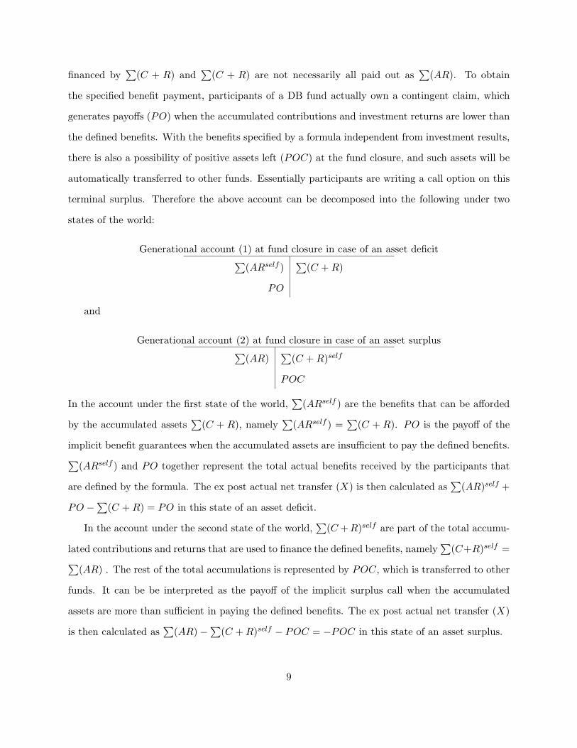
financed by∑

(C + R) and∑

(C + R) are not necessarily all paid out as∑

(AR). To obtain

the specified benefit payment, participants of a DB fund actually own a contingent claim, which

generates payoffs (PO) when the accumulated contributions and investment returns are lower than

the defined benefits. With the benefits specified by a formula independent from investment results,

there is also a possibility of positive assets left (POC) at the fund closure, and such assets will be

automatically transferred to other funds. Essentially participants are writing a call option on this

terminal surplus. Therefore the above account can be decomposed into the following under two

states of the world:

Generational account (1) at fund closure in case of an asset deficit∑(ARself )

∑(C +R)

PO

and

Generational account (2) at fund closure in case of an asset surplus∑(AR)

∑(C +R)self

POC

In the account under the first state of the world,∑

(ARself ) are the benefits that can be afforded

by the accumulated assets∑

(C + R), namely∑

(ARself ) =∑

(C + R). PO is the payoff of the

implicit benefit guarantees when the accumulated assets are insufficient to pay the defined benefits.∑(ARself ) and PO together represent the total actual benefits received by the participants that

are defined by the formula. The ex post actual net transfer (X) is then calculated as∑

(AR)self +

PO −∑

(C +R) = PO in this state of an asset deficit.

In the account under the second state of the world,∑

(C +R)self are part of the total accumu-

lated contributions and returns that are used to finance the defined benefits, namely∑

(C+R)self =∑(AR) . The rest of the total accumulations is represented by POC, which is transferred to other

funds. It can be be interpreted as the payoff of the implicit surplus call when the accumulated

assets are more than sufficient in paying the defined benefits. The ex post actual net transfer (X)

is then calculated as∑

(AR)−∑

(C +R)self − POC = −POC in this state of an asset surplus.

9

At the time of fund establishment before guarantees or surplus options are realized, the gener-

ational account looks like:

Generational account (3) at the fund establishment

V (AR) V (C +R)

V (PO) V (POC)

At the contracting time, the economic value of contributions and investments equals the eco-

nomic value of the accrued rights, V (AR) = V (C + R), as the contribution rate is determined

in such a way that the defined benefits can be fully financed (even though ex post they are not

often matched). The economic value of the option payoffs is simply their respective market prices,

V (PO) = Pgua and V (POC) = Pcall. Therefore we can see that the net transfer ex ante is

V (X) = V (AR) + V (PO)− V (C +R)− V (POC) = Pgua − Pcall

The price of the guarantee (Pgua) and the price of the call (Pcall) are derived from the pension

deal once the fund has set its contribution, indexation and investment policy. If the price of the

guarantee (Pgua) is larger than the price of the call (Pcall), then the fund has a positive net transfer,

meaning the fund is a net receiver. If the value of the guarantee is smaller than the value of the

call, then the fund has a negative net transfer, meaning the fund is a net giver. Whether the net

transfer is 0 determines whether this DB deal is a fair contract. This also highlights the importance

of explicitly pricing the options in designing a fair plan, as put forward by Kocken (2006). In this

paper we try to price this guarantee and surplus call so that a generational DB fund can explicitly

trade them and strike a fair deal for its participants. The existence of the guarantee and the

call reveals the mechanism for intergenerational risk sharing in a generational plan, because the

deficiency in assets is made up by guarantee providers and the surplus of terminal assets is left to

other generations. The magnitude of this risk sharing is Pcall + Pgua.

The above account is only for one generational fund. At the pension plan level, the consolidated

account is simply the aggregation of all individual accounts for each generational fund. Since

options are traded within the pension plan at their fair prices or market consistent prices, the

total net transfer (X) will be 0, making a generational plan with option arrangement a sustainable

10

system. The zero-sum makes the generational plan resembles the collective plan that they are both

a self-contained system. What distinguishes a generational plan from a collective one is that the

transfers between generations are explicitly priced in the generational plan. Such prices quantify

intergenerational risk sharing and contribute to the sustainability of a pension plan. In a collective

plan there exist transfers between generations, but they are implicit and can lead to differential

treatment to different generations. As a consequent some generations may opt out of the plan.

Our analysis of the generational account combines ideas from previous studies, but also distin-

guishes itself in the following aspects. Kocken (2006) detects implicit options embedded in pension

contracts but does not assign them to different generations. Hoevenaars & Ponds (2008) introduce

the generational account to study the transfers, but their focus is the change of the value of an

generational account due to a change of the pension deal. In addition, they study the value changes

for a generational account for a time window of 20 years, while we study the value transfers over

the entire life of a generation. Cui, de Jong & Ponds (2009) discuss the value transfers between

generations within a collective plan in the context that all generations apply the uniform poli-

cies in contribution, investment, and indexation. We show the value transfer from one particular

generation, and this transfer varies to the particular pension deal chosen by the generation.

3 Option payoff structures

The last section shows the setup of the guarantee and surplus call option in a DB generational fund,

this section tries to value these options by modeling the development of the assets and liabilities

of a generational conditional DB fund. We explain how the values of the contingent claims are

determined. Guarantees to pension benefits can take two forms: minimum rate of return guaran-

tees and minimum benefit guarantees as summarized in Lachance & Mitchell (2003). In our setup,

the guarantees are of the second form. We allow for three types of guarantees: (1) guaranteeing

nominal pension benefits, based on life-time average salaries and a replacement rate; (2) guaran-

teeing the accrued pension rights including previously granted conditional indexation rights; and

(3) guaranteeing unconditional real pension benefits that are fully indexed to the inflation rates.

11

3.1 A conditional DB generational fund

We use a representative individual for a generation to model the development of a generational

fund. Assume a participant enters the labor market at T0, retires at Tr, and dies at Td. He earns

a flat salary (S0).

The assets (At) grow due to contribution collections (ptS0) and investment returns (rA,t).

At = At−1(1 + rA,t) + ptS0 (1)

During the working years the liabilities change due to the change in accrued rights (ARt) and

the corresponding yield curve.

Lt =

Td−Tr∑n=0

ARt

(1 + yTr−t+n,t)Tr−t+n(2)

where yTr−t+n,t is the yield of maturity Tr − t+ n at time t.

ARt refers to accrued rights at time t, it is the future annual benefits that is entitled to partic-

ipants since their retirement. In year 1 the accrued rights are AR1 = NAR(1+ ind1). From year 2

onwards until retirement the accrued rights are given by ARt+1 = (ARt +NAR)(1 + indt+1). indt

is the indexation rate. NAR is the newly accrued rights for one year of service and time indepen-

dent. If RR is the replacement rate, then for every year of service NAR is RR/(Tr − T0) ∗S0. The

indexation rate in this study is bounded within [0,100%], so the accrued rights is always between

the nominal rights and real rights.

Upon retirement (t = Tr), the fund starts to pay out benefits as defined in ARt and still invests

the rest. So the assets on the one hand decrease with the benefit payments, while on the other

hand increase with the investment returns, and they follow

At = At−1(1 + rA,t)−ARt (3)

No new rights are accrued as of retirement, NAR = 0. The total accrued rights only increase

with indexation ARt+1 = ARt(1+ indt+1). The value of the fund liabilities is the discounted value

12

of the benefit payments with a declining amount of years.

Lt =

Td−t∑n=0

ARt

(1 + yn,t)n(4)

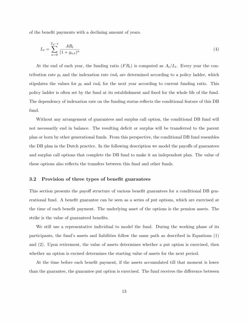
At the end of each year, the funding ratio (FRt) is computed as At/Lt. Every year the con-

tribution rate pt and the indexation rate indt are determined according to a policy ladder, which

stipulates the values for pt and indt for the next year according to current funding ratio. This

policy ladder is often set by the fund at its establishment and fixed for the whole life of the fund.

The dependency of indexation rate on the funding status reflects the conditional feature of this DB

fund.

Without any arrangement of guarantees and surplus call option, the conditional DB fund will

not necessarily end in balance. The resulting deficit or surplus will be transferred to the parent

plan or born by other generational funds. From this perspective, the conditional DB fund resembles

the DB plan in the Dutch practice. In the following description we model the payoffs of guarantees

and surplus call options that complete the DB fund to make it an independent plan. The value of

these options also reflects the transfers between this fund and other funds.

3.2 Provision of three types of benefit guarantees

This section presents the payoff structure of various benefit guarantees for a conditional DB gen-

erational fund. A benefit guarantee can be seen as a series of put options, which are exercised at

the time of each benefit payment. The underlying asset of the options is the pension assets. The

strike is the value of guaranteed benefits.

We still use a representative individual to model the fund. During the working phase of its

participants, the fund’s assets and liabilities follow the same path as described in Equations (1)

and (2). Upon retirement, the value of assets determines whether a put option is exercised, then

whether an option is excised determines the starting value of assets for the next period.

At the time before each benefit payment, if the assets accumulated till that moment is lower

than the guarantee, the guarantee put option is exercised. The fund receives the difference between

13

the assets available and the guarantee. This amount is also the payoff of the guarantee option. Then

the asset value for the next period becomes 0. If the asset value is not lower than the guarantee,

the fund assets will continue as specified in Equation (3). The following lists the payoff of the

guarantees, the development of the asset value and the accrued rights during the payout phase.

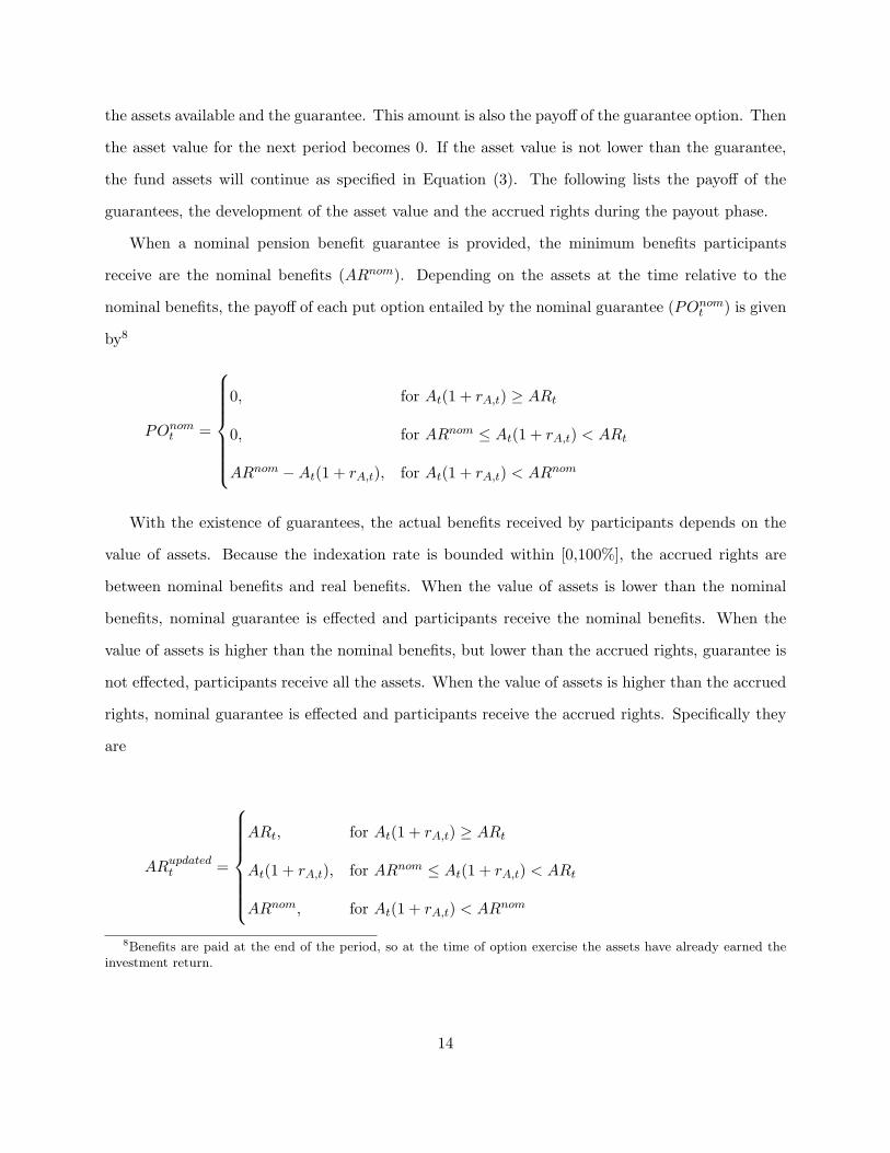
When a nominal pension benefit guarantee is provided, the minimum benefits participants

receive are the nominal benefits (ARnom). Depending on the assets at the time relative to the

nominal benefits, the payoff of each put option entailed by the nominal guarantee (POnomt ) is given

by8

POnomt =

0, for At(1 + rA,t) ≥ ARt

0, for ARnom ≤ At(1 + rA,t) < ARt

ARnom −At(1 + rA,t), for At(1 + rA,t) < ARnom

With the existence of guarantees, the actual benefits received by participants depends on the

value of assets. Because the indexation rate is bounded within [0,100%], the accrued rights are

between nominal benefits and real benefits. When the value of assets is lower than the nominal

benefits, nominal guarantee is effected and participants receive the nominal benefits. When the

value of assets is higher than the nominal benefits, but lower than the accrued rights, guarantee is

not effected, participants receive all the assets. When the value of assets is higher than the accrued

rights, nominal guarantee is effected and participants receive the accrued rights. Specifically they

are

ARupdatedt =

ARt, for At(1 + rA,t) ≥ ARt

At(1 + rA,t), for ARnom ≤ At(1 + rA,t) < ARt

ARnom, for At(1 + rA,t) < ARnom

8Benefits are paid at the end of the period, so at the time of option exercise the assets have already earned theinvestment return.

14

Accordingly the value of assets for the next period depends on how much benefits are actually

paid. When the assets are less than the nominal benefits, the fund pays the nominal benefits by

using the money received from the guarantee. The assets for the next period is 0. In sum they are

given by

At+1 = At(1 + rA,t)−ARupdatedt =

At(1 + rA,t)−ARt, for At(1 + rA,t) ≥ ARt

0, for ARnom ≤ At(1 + rA,t) < ARt

0, for At(1 + rA,t) < ARnom

When an accrued pension rights guarantee is provided, the indexation won’t be negative and

the accrued pension rights (ARt) are protected from any current and future cutdown. Participants

receive what they have accrued, namely ARupdatedt = ARt. The payoff of this guarantee is

POARt =

0, for At(1 + rA,t) ≥ ARt

ARt −At(1 + rA,t), for At(1 + rA,t) < ARt

The assets for the next period becomes

At+1 = At(1 + rA,t)−ARupdatedt =

At(1 + rA,t)−ARt, for At(1 + rA,t) ≥ ARt

0, for At(1 + rA,t) < ARt

When a real pension benefit guarantee is provided, participants always receive the real benefits,

ARupdatedt = ARreal

t , as the real benefits are the highest possible benefits participants can receive9.

The real benefits are fully indexed to all the inflation rates over time, ARrealt+1 = (ARreal

t +NAR)(1+

πt+1) and πt is the inflation rate. The payoff of this guarantee only depends on the comparison

9As indexation rate is not larger than 100%, ARt is not higher than ARrealt .

15

between the assets and the real benefits. It is given as

POrealt =

0, for At(1 + rA,t) ≥ ARreal

t

ARrealt −At(1 + rA,t), for At(1 + rA,t) < ARreal

t

The assets for the next period is

At+1 = At(1 + rA,t)−ARupdatedt =

At(1 + rA,t)−ARrealt, for At(1 + rA,t) ≥ ARreal

t

0, for At(1 + rA,t) < ARrealt

We give a numerical example. Suppose now the fund is at the point to pay out its first benefits.

The assets accumulated till this moment is e40, 000. The nominal and real pension rights are

respectively e21, 000 and e80, 000, and the accrued rights till this moment is e60, 000. At this

point, the first put option contained in a guarantee is to be expired. If the fund holds a nominal

guarantee, because the value of assets is larger than the minimum guarantee of nominal benefits,

this first put option is not exercised, the payoff of the nominal guarantee at this moment is 0.

Participants should get the accrued rights, but the fund assets are not enough. Participants then

receive what the fund can afford, which is e40, 000. The starting value of assets for the next

period is 0. If the fund holds an accrued rights guarantee, because the value of assets is smaller

than the accrued rights, the first put option contained in this guarantee is exercised, payoff of

the accrued rights guarantee at this moment is e(60, 000 − 40, 000). Participants receive accrued

rights,e60, 000. The starting value of assets for the next period is 0. If the fund has a real benefit

guarantee, because the value of assets is smaller than the real rights, the first put option contained

in this guarantee is exercised, payoff of the real guarantee at this moment is e(80, 000 − 40, 000).

Participants receive real benefits, e80, 000. The starting value of assets for the next period is 0.

The value of liabilities is calculated in the same way as described in Equation (4).

16

3.3 Selling the fund surplus

As mentioned, the generational fund is an independent fund. At the fund disclosure when all

participants die, the fund is dissolved automatically. If there are any assets left, then they would

be automatically transferred to the other funds or to the plan level for central planning. From the

perspective of the generational fund, this potential surplus is given away without compensation.

To avoid wasting resources, the fund can sell a call option on its terminal surplus. This call option

entitles the buyer any positive assets left with the fund at its closure. Using the previous setup the

payoff of this call option (POC) is

POC = max(0, ATd(1 + rA,Td

)−ARupdatedTd

)

As the value of assets varies to the guarantee arrangement, the value of the call also differs for

various guarantee arrangements.

4 Empirical methodology

Benefit guarantees and surplus options are traded among generational funds within a common par-

ent plan, which forms an internal market. We assume a complete market that all states of liabilities

can be replicated within this internal market. We apply the risk neutral technique introduced by

Cox & Ross (1976). It says that in the absence of arbitrage opportunities, there exists a risk neutral

probability such that

V (t, Tr, Td) = e−rft(T−t)Et[

T=Td∑T=Tr

PO(T )] (5)

The left hand side is the value of the guarantees at time t and the guarantees are effective from the

retirement date (Tr) until the death date (Td). The guarantee functions like a number of Td−Tr put

options. rft is the risk free rate at t. Et is the expectation taken at time t and under risk-neutral

measure. In its bracket is the sum of options which each has a payoff at the time of each benefit

payment. These payoffs are specified in the previous section. In the same way, the value of the

17

surplus call at time t and expires at Td is

V C(t, Td) = e−rft(Td−t)Et[POC(Td)] (6)

The payoffs are generated in a risk neutral world when all investments are earning a risk free

rate. We specify the following stochastic process for stock returns, bond returns, yield curve and

inflation in the risk-neutral world where risk premium is 0. We use the Vasicek model (1977) to

model the risk free rate. We choose this approach for yield curve modeling because it is based

on the no-arbitrage principle and suitable for pricing purpose. As the Vasicek model does not

preclude a negative rate, we apply this model to the real risk free rate. Then according to Fisher’s

hypothesis, the nominal short rate is the sum of the real rate and expected inflation rate. This

two-factor approach for the nominal rate is also applied by Campbell & Viceira (2001). Specifically,

the real rate (rt) and expected inflation (πt) respectively follow:

rt+1 = r + ϕ(rt − r) + ϵrt+1

πt+1 = π + κ(πt − π) + ϵπt+1

r and π are the long term means of the real rate and expected inflation. ϕ and κ are mean reversion

coefficients of the real rate and expected inflation. The risk free rate is rft = rt + πt.

According to the expectation theory, a long term rate is the average of expected future short

rates. Therefore we have the yield for m periods at t as

ym,t = r + π +1− ϕm

m(1− ϕ)(rt − r) +

1− κm

m(1− κ)(πt − π)

Accordingly the return of a zero-coupon bond with m years to maturity follows

bondm,t =pricem−1,t+1

pricem,t− 1 = exp(mym,t − (m− 1)ym−1,t+1)− 1

We assume pension funds invest in 10-year zero bonds. Assuming stock prices follow a lognormal

18

distribution, then the annual stock return follows

stockt = exp(rft − σ2/2 + σϵst )

ϵrt+1, ϵπt+1, ϵ

st are shocks to the real rate, expected inflation and stock return respectively. Each

follows a standard normal distribution and is independent from each other.

Because the payoffs of the guarantees and the surplus call option are path-dependent on the

development of assets and liabilities, which are mediated by the contribution, indexation and in-

vestment polices set in the pre-specified policy ladder, it is hard to derive a closed-form solution

for the values. We make a numeric valuation with a Monte Carlo simulation. Such simulation

approach has been applied in various pension contexts in different countries10.

Specifically, we simulate 1000 paths for stock returns and yield curves through the lifetime of

a generational fund. From the simulated yield curves we derive bond returns, together with the

simulated stock returns, we get the value for assets. Discounting accrued rights with the simulated

yield curves, we get the value for liabilities. Accordingly we obtain 1000 scenarios of option payoffs.

Discounting the payoffs at the risk free rates we get the present value of the options.

The values of all options will be determined at the time of its establishment as soon as the

fund has announced its contribution, indexation and investment policy. A fund can only trade

such options at this time by signing a contract with counter parties. However, they can fulfill the

payment during the whole working phase. Of course the price will be higher the later they buy due

to the time value of money.

We collect all the data in an annual frequency over the period between year 1954 and 200711.

We take the 3-month US T-bill rate for the short nominal rate. The annual inflation rate is

calculated from US Consumer Price Index-All Urban Consumers. This realized inflation rate is

used to back out the expected inflation assuming an AR(1) process. Then the real rate is obtained

as the difference between the nominal rate and the expected inflation rate according to the Fisher

10Consult Pennacchi (1999) for public and private pension funds guarantee in Uruguay and Chile, Feldstein &Ranguelova (2000) for DC plan guarantee in the US, Lachance et al. (2003) for DC to DB conversion, Kocken (2006)for option valuation in pension contracts.

11This is the period when all the data are available.

19

hypothesis. From the Center for Research and Security Prices (CRSP) of the University of Chicago

we get the stock return (including dividends), which is for a value-weighted portfolio including all

stocks traded on the NYSE, NASDAQ, and AMEX. The parameter estimates are shown in Table

1.

5 Prices of guarantees and the call option

The options are designed to handle the investment risk, longevity risks, and labor income risks that

lead to the mismatch between assets and liabilities. Firstly we will present two sets of prices in a

baseline case when only diversifiable financial risks are considered. One set of prices is under the

assumption of a deterministic labor income, and the other is under a stochastic labor income. Then

starting from the base prices under deterministic labor income, we go on to show the sensitivities

of these prices when there is a generation-long shock to the financial market reflected by a higher

market volatility of the stock market; and the sensitivity when there is a longevity risk reflected by

a stochastic life expectancy.

5.1 Base prices under a deterministic labor income

In the baseline case, the uncertainty of the assets and liabilities of a generational fund comes only

from the financial market risks, which are represented by the yield curve and the stock market

described in the previous section. The assumptions on the fund and participants are specified in

Table 2. The entire life of a generational DB fund is 55 years. The first 40 years are the working

phase when the fund collects contributions, and the later 15 years are the retirement phase where

the fund pays out retirement benefits. The average of the participants earn a flat salary (S0) over

the working years at e30,000. All cash flows occur at the end of each year, namely participants

get salary, pay contributions and receive pension benefits all at the end of the year. The policy

ladder concerning contribution and indexation policy is defined in Figure 1. The contribution rate

is adjusted within a range of [-5%, 5%] around the base rate according to the funding ratio. In the

beginning when the funding ratio is above 6, the contribution rate is 5% lower than the base rate,

and is 5% higher when the funding ratio is lower than 1. Over time the upper bound of the funding

20

ratio linearly declines to 2 at the time of retirement. The upper bound is set initially high at 6 in

the consideration of the mechanically low starting liabilities which otherwise lead to no contribution

requirement. Investment policy is set constant at 50% stocks and 50% bonds during the working

and retirement phase. The base contribution rate is determined in a actuarially fair way. It is

solved from∑Td

t=1 pS0(1+rt)−t =

∑Tdt=Tr

S0RR(1+rt)−t, which says the lifetime individual pension

entitlements equals to lifetime individual pension contributions. Based on the historical mean real

rate of 1.27% as the discount rate (rt)12 and 70% replacement rate (RR), the base contribution

rate (p) is set at 18.38%. The dynamics of the fund over time is shown in Figure 2 depicting the

average simulated contribution rate, indexation rate and various types of pension rights.

Panel A in Table 3 shows the prices of the three types of benefit guarantees and the surplus

call under the three types of guarantees at the time of the first contribution collection. When only

the nominal pension benefit is guaranteed, namely participants can get at least 70% of the annual

salary after retirement, the guarantee costs for one time 4.17% of the yearly salary when purchased

at age 26, the time of the first contribution payment. If paid in annual installment over the whole

working years, it is only 0.1%13 of the salary. Compared to the base contribution rate of 18%, this

nominal guarantee is only a marginal addition to the pension cost. The average paid benefits are

e65,510, far over the nominal guarantee of e21,000. It reflects the fact that the nominal guarantee

is not exercised most of the time. This low cost is expected because a real rate 1.27% is used as

the discount rate to set the base contribution rate to afford the real benefits.

When the accrued pension rights are guaranteed, namely, participants at least maintain the

level of the previous year’s benefits, this guarantee costs for one time 12.11% of the yearly salary.

Such guarantee can provide an average annual benefit of e68,219, about 86% of the real benefits.

When the real pension benefit is guaranteed, where participants get inflation-proof benefits,

it costs considerably 60% of the yearly salary. If paid in annual installment over 40 years, this

guarantee costs an annual amount of 1.5% of the salary.

12Pointed out in Queisser & Whitehouse (2006), the discount rate is a central and contentious issue in settingcontribution rate. In general there are three possible choices for the discount rate. They are market rate of return,riskless interest rate and fiscally sustainable rate. Here we choose the real riskfree rate to make a conservativecalculation of contribution rate.

13=4.17%/40.

21

Selling a call option on the surplus of the terminal assets, a generational fund can avoid wasting

the upside potential of its assets to generate an extra income to pay for the benefit guarantees. In

general, the value of this call option on the fund surplus goes in a different direction from the value

of the benefit guarantee. When the fund becomes affluent, the value of the guarantees decreases

while the value of the call increases.

When a fund is provided with a nominal guarantee, the call option it can issue at the fund

establishment is worthy of 49.31% of the annual salary. For a fund provided with an accrued rights

guarantee, the call option is worth the same value. This is because the payoff of a call option

only counts the upside potential, and this upside potential is the same for a fund with a nominal

guarantee and a fund with an accrued rights guarantee. The conditional DB plan defines that

participants get a high indexation when the value of assets are high. Therefore when the assets

develop to its up state, participants receive the same granted indexation when the fund is provided

with either a nominal or an accrued rights guarantee. The assets accordingly follow the same path

in the up states, leading to the same value of the surplus call option.

For a fund provided with a real guarantee, the call option is worth 47.31%, not much lower

than the call under the other two guarantee types. This is because the base contribution rate is

set to aim for real benefits, which most of the time enables the fund to grant a high indexation.

This leads to little difference between the surplus under a real guarantee and the surplus under the

other guarantees.

5.2 Base prices under a stochastic labor income

The previous case assumes a deterministic labor income. Now we incorporate an exogenous la-

bor income risk14. The shocks in the labor income can influence the contributions and the asset

accumulation, accordingly will influence the accrued rights and liabilities.

We apply a simple process for the labor income as St = E(S) ∗ (1 + s+ ξt)15. St is the income

14Here we abstract from the endogeneicity that labor supply can vary with labor income shocks and the correlationbetween the labor income shock and the investment return shock.

15Often used in literature is that labor income follows log normal distribution such as in Carroll (1997)and Viceira(2001) that St+1 = Stexp(s+ξt+1). But in order to make it comparable to the baseline case we assume labor income isnormally distributed rather than being lognormally distributed, because the later assumption will lead to an increasein the expected labor income even when the error term has a mean of 0.

22

flow at year t. s is the expected income growth rate, and ξt follows NIID(0, σ2ξ ). For the simulation

and comparison purpose we set S0 = 30, 000, s = 0 and σξ = 0.116.

The second set of prices in Panel A of Table 3 shows that the prices do not change much from the

base case with a deterministic labor income. This is because the average income is the same in both

cases and after 40 years of accumulation the distribution of assets and liabilities are comparable at

the time of retirement in both cases. In addition, the labor income risk does not influence the fund

dynamics after retirement when the guarantee starts to be effective. Therefore a random income

shock from a standard normal distribution has negligible impact on the option prices.

5.3 Sensitivities to non-diversifiable investment and longevity risks

The base prices of the guarantees and the call are based on the assumptions summarized in Table

2. This section relaxes some of the assumptions and considers two non-diversifiable risks that the

generation has to share with other generations, namely the uncertainty on the financial market and

the life expectancy.

There is a possibility that one generation could suffer from a life-long shock from the financial

market so that the generation cannot diversify such risk away within itself. We apply an alternative

value for the stock market volatility to reflect this risk. We calculate the volatility of stock returns

within a 20-year window during our sample period and find the highest volatility is 18.33%, which is

a 22% increase from 15.06% for the base case. The investment risk directly influences the volatility

of assets both during the working phase and the post-retirement phase. This causes considerable

increases in the prices of the guarantees and the call, ranging from a 14% to a 43% increase. Figure

3 compares the payoffs of three types of guarantees under this scenario with the payoffs under the

base case. There is an increase in the payoffs irrespective of the guarantee type. Relatively the

percentage increase in the price of the nominal benefit guarantee is the highest, and the percentage

increase in the price of the real benefit guarantee is the lowest.

The average annual pension benefits received by the participants under the macro-investment

risk, seen in the last two columns of Table 3, are lower than the base case because of the no catch-up

16This is taken from Viceira (2001).

23

indexation in our pension design. More volatile assets under the investment risk will miss some

indexation which will not be made up later even when the value of assets picks up.

The base contribution rate is set based on the life expectancy of the generation. The uncertainty

in the life expectancy is a non-negligible risk. We incorporate this risk by making the life expectancy

a random variable from a normal distribution with a mean of 80 years and a standard deviation of

2 years.

When the generation has a lower life expectancy than the expected, the extra surplus assets

are transferred to other funds who bought a surplus call from this fund. When the generation

has a longer life expectancy than the expected, the fund policy is set as follows. For the years

after the expected life expectancy, no investment is made and no indexation is given. Under the

nominal guarantee, the fund aims to pay what it can afford, with the order of firstly the accrued

rights, secondly the less indexed rights, and lastly the nominal benefits. Under the accrued rights

guarantee, the fund always pay the accrued rights as participants have accrued till the last year

of their expected life expectancy. Under the real guarantee, the fund still pays inflation-indexed

benefits, including the inflation rate for these extra years.

Panel B in Table 3 shows that this longevity risk increases the prices of the guarantees con-

siderably. Figure 4 compares the average payoffs of three types of guarantees under this scenario

with the payoffs under the base case. In the base case, the payoffs stop at the expected death age

of 80. In the longevity case, the payoffs for short-lived years are on average lower than the payoffs

for long-lived years. Therefore the guarantee often pays more and accordingly more valuable when

there exists uncertainty on the life expectancy.

The impact of the longevity risk on the call option is negligible. This is because the call only

concerns the terminal assets when obligations to all participants are filled. The possibility of both

out-living and under-living the expected age leads to a non-significant change in the average value

of the terminal assets.

24

5.4 Net Transfers

A generational fund accommodates the needs of a particular generation. Buying a benefit guarantee

protects its participants from non-diversifiable generation-specific shocks. Selling a call option on

the fund surplus avoids under-consumption. Recalling the generational account of a DB deal at

the fund establishment, the net transfer a prior is determined by the difference between the value

of the guarantee and the value of the call. A conditional DB deal in our numerical example is a

net giver when it is provided with either a nominal or an accrued rights guarantee, meaning this

fund transfers net positive values to other funds because the call it sells has a higher value than

the guarantee it receives. For a conditional DB deal with a real benefit guarantee, the fund is a net

receiver, as the real guarantee it receives is more valuable than the call it sells. The above results

remains when the additional investment risk and longevity risk are considered.

To make the generational DB deal a fair deal, we should equalize the value of the guarantee

and the surplus call. This can be done via a change in the contribution, indexation or investment

policy, or simply pay or receive the difference between the price of the guarantee and the price

of the surplus call. Here we give an example of doing so via a change in the contribution policy.

Table 4 reports the break-even base contribution rate that equalizes the value of the guarantee and

the value of the surplus call when the underlying fund has the characteristics defined in Table 2.

With this base contribution rate, a generational fund with a conditional DB deal does not have to

pay a cash outflow explicitly for the guarantee or receive cash inflow explicitly for the call. The

break-even base contribution under the nominal guarantee is 10.16%. It means if a generational

fund whose characteristics are defined as in the assumptions in Table 2 adopts a conditional DB

deal with a nominal guarantee, then this DB deal is a fair deal if it sets its base contribution rate

at 10.16%. It will be net giver(receiver) if its base contribution rate is higher(lower) than 10.16%.

For a fund with an accrued rights and a real benefit guarantee, the break-even base contribution

rate is respectively 13.09% and 19.28%.

Comparing the value of the guarantee or the call under three types of guarantees, we find the

value is highest in the case of a real guarantee provision. This reveals that the risk sharing among

generational funds is the highest when a real benefit guarantee is traded, and is the lowest when

25

only nominal benefit guarantee is traded.

6 Conclusion and discussion

A generational pension fund enables customized fund management in contribution, indexation and

investment policies, facilitates risk management of a pension fund geared to the preference of a

particular generation, and frees pension sponsors from unwanted risks. To further improve the

welfare of participants, guaranteeing pension benefits can be desirable. As a generational fund is

financially independent, the upside potential of its terminal assets should also be sold to avoid under-

consumption. The arrangement of such options provides a mechanism for intergenerational risk

sharing, and this chapter tries to quantify this risk sharing by pricing the options. In the collective

plan, such options are implicitly embedded in the contract and can hardly be quantified. Our design

of option trading and their valuation in the setup of a generational plan makes intergenerational

risk sharing more explicit and transparent, and can be used as a reference to the risk sharing in

the current collective plan.

Applying risk-neutral and simulation techniques, we show that with a base contribution rate

determined by using a real rate as the discount rate the nominal and accrued rights guarantees

are relatively cheap. The one-time cost of the nominal benefits guarantee is 4%, the accrued rights

guarantee is 12% and the real rights guarantee is 60% of the yearly salary. A call option written

on the surplus of the terminal assets is worth about 50% of the yearly salary for all types of the

benefit guarantee. We consider another base case with a stochastic labor income that has the same

expected annual salary as in the deterministic labor income case. This has negligible impact on

the option prices as labor income shocks only influence the fund assets till the retirement.

We also show the sensitivity of the option prices when some of the non-diversifiable risks are

incorporated. We reflect the generation-long shock in investment by increasing the volatility of the

stock returns to the historic highest in our sample period. This investment risk directly influences

the volatility of the fund asset accumulation both during the working phase and the retirement

phase. This causes considerable increases in the prices of all guarantees and the surplus call.

We reflect the longevity risk by making the life expectancy a random variable from a normal

26

distribution. The uncertainty of the life expectancy leads to only a marginal change in the value

of the surplus call due to the two-side possibilities of realized life-time. However it increases the

prices of all benefit guarantees considerably.

The explicit pricing of the contingent claims help to identify whether a deal is a fair deal ex

ante. To make a fair deal in a generational plan, a change can be made in the fund policies

concerning contribution, indexation, and investment, or a money difference between the prices of

the guarantee and the surplus call can be paid. Regarding the DB deal in our example, we find that

respectively at a break-even base contribution rate of 10.16%, 13.09% and 19.28%, a generational

fund featured in our base case with a deterministic labor income does not have to make explicit

cash flows for the options under nominal, accrued rights and real guarantee provisions. At these

rates, a conditional DB deal is a fair deal. The break-even values of the guarantees or the call also

reflect that the intergenerational risk sharing is the highest when a real benefit guarantee is traded

among generational funds.

In our evaluation, we actually assume a partial equilibrium that a generation only buy the

guarantee and sell a surplus call from and to a young or possibly an unborn generation. Yet in a

complete equilibrium, this generation can also be the seller of the guarantee and the buyer of the

surplus call to and from the current elder generations. In this case we should apply an overlapping

generation model with three generations, where each have their own deal concerning investment,

contribution and indexation policies.17 Nevertheless, this chapter provides a framework how the

contingent claims can be priced explicitly to make a fair deal.

The valuation of the options traded among generational funds is done under the complete market

assumption. This is a very restrictive assumption as replicating the option payoffs and a market

for continuous trading of the contingent claims can be hard to implement in practice. Hence our

current estimation only provides the first proximate of their market values. The future research

can be in the direction of the valuation of such options under an incomplete market.

17Then there will be a concern over the credibility of the guarantee provider. Our primary solution is having theparent plan acting as the intermediary to execute the trading and making the payoff on behalf of the generationalfunds.

27

References

Blake, D., A. Cairns & K Dowd (2006), ‘Living with mortality: Longevity bonds and other

mortality-linked securities’, British Actuarial Journal 12(1), 153–197.

Campbell, J.Y. & L.M. Viceira (2001), ‘Who should buy long-term bonds?’, The American Eco-

nomic Review 91(1), 99–127.

Carroll, Christopher D. (1997), ‘Buffer-stock saving and the life cycle/permanent income hypothe-

sis’, Quarterly Journal of Economics 112, 1.

Cox, John C. & Stephen A. Ross (1976), ‘The valuation of options for alternative stochastic pro-

cesses’, Journal of Financial Economics 3, 145.

Cui, Jiajia, Frank de Jong & Eduard Ponds (2009), Intergenerational risk sharing within funded

pension schemes, Technical report, Network for Studies on Pensions, Aging and Retirement,

The Netherlands.

Feldstein, Martin & Elena Ranguelova (2000), ‘Accumulated pension collars: A market approach to

reducing the risk of investment-based social security reform’, NBER Working paper No.7861,

August.

Hoevenaars, Roy P.M.M. & Eduard H.M. Ponds (2008), ‘Valuation of intergenerational transfers

in funded collective pension schemes’, Insurance: Mathematics and Economics 42, 578–593.

Kocken, Theo P. (2006), Curious Contracts: Pension Fund Redesign for the Future, PHD thesis,

Tutein Nolthenius.

Lachance, Marie-Eve & Olivia S. Mitchell (2003), ‘Understanding individual account guarantees’,

Working paper, University of Michugan Retirement Research Center and NBER.

Lachance, Marie-Eve, Olivia S. Mitchell & Kent Smetters (2003), ‘Guaranteeing defined contribu-

tion pensions: The option to buy back a defined benefit promise’, The Journal of Risk and

Insurance 70(1), 1–16.

28

Pennacchi, George G. (1999), ‘The valuation of guarantees on pension fund returns’, The Journal

of Risk and Insurance 66(2), 219–237.

Ponds, Eduard (2003), ‘Pension funds and value-based generational accounting’, Journal of Pension

Economics and Finance 2(3), 295–325.

Queisser, Monikaand & Edward Whitehouse (2006), ‘Neutral or fair? actuarial concepts and

pension-system design’, OECD Social, Employment and Migration, working paper NO. 40.

Smetters, Kent (2002), ‘Controlling the cost of minimum benefit guarantees in publich conversions’,

Pension Economics and Finance Journal 1, 9–33.

Viceira, Luis M. (2001), ‘Optimal portfolio choice for long-horizon investors with nontradable labor

income’, Journal of Finance 56, 433.

29

Table 1: Parameter estimates based on annual observations during 1954-2007Real world Risk neutral world σ

Real rate r=1.27% r=1.27% 1.50 %ϕ=0.56 ϕ=0.56

rT=1.43%(initial value for simulation)

Expected inflation π=4.16% π=4.16% 1.83%κ=0.78 κ=0.78

πT=4.12%(initial value for simulation)

Stock return 10.81% 5.43% 15.06%r and π are the long term means, ϕ and κ are the mean reversion coefficients of real rate andexpected inflation.

Table 2: Assumptions for baseline scenariosParameters Values

Age of labor entry 25Retirement age 65Death age 80Starting annual salary e30,000Annual salary growth rate 0Replacement rate 70%Investment policy constant 50% in stocks and 50% in bondsRisk free rate 5.43%Base contribution rate 18.38%

30

Table 3: Value of the guarantees and the call across different scenariosGua. type Guarantee Call Ann. B. % of real B.Panel A

Base case with a deterministic labor income

Nominal guarantee 4.17 49.31 65,510 83.45Accursed rights gua. 12.11 49.31 68,219 85.84Real guarantee 59.34 47.31 83,652 100

Base case with a stochastic labor income

Nominal guarantee 4.17 49.39 65,517 83.45Accursed rights gua. 12.10 49.39 68,225 85.84Real guarantee 59.32 47.32 83,652 100

Panel B

Sensitivity to investment risk

Nominal guarantee 5.98 60.70 63,709 81.32(43.47% ) (23.09%)

Accursed rights gua. 15.99 60.70 67,028 84.35(32.11%) (23.09%)

Real guarantee 67.69 57.99 83,652 100(14.08%) (22.58%)

Sensitivity to longevity risk

Nominal guarantee 5.42 49.64 63,981 81.69(29.95%) (0.66%)

Accursed rights gua. 17.65 49.64 67,170 84.4(37.55%) (0.66%)

Real guarantee 66.92 44.49 84,423 100(12.78%) (-5.96%)

The table reports the prices of the nominal benefit, accrued rights, and real benefit guaranteesand the surplus call option by simulating a generational conditional DB fund. Panel A reportsthe prices for the base cases respectively with a deterministic and a stochastic labor income. Theassumptions for the base case are specified in Table 2 and Figure 1. Panel B reports the priceswhen the uncertainties in the volatility of the stock market and the life expectancy are considered.Specifically, in considering the investment risk we increase the volatility of the stock market tothe highest 20-year volatility in the sample period. In considering the longevity risk, we make thelife expectancy a random variable with a nominal distribution that has a mean of 80 years anda standard deviation of 2 years. ”Guarantee” and ”Call” are the one-time price of the benefitguarantee and the call respectively at the time of first contrition collection, expressed as as apercentage of the average annual salary. ”Ann. B” displays the average annual benefits expressedin ethat participants receive since their retirements, and its average percentage of the fully indexedbenefits/real benefits is shown in the last column. Numbers in brackets are the change in valuewhen compared with the base case with a deterministic labor income

31

Table 4: Break-even base contribution rateContribution rate Value of guarantee Value of call

Nominal guarantee 10.16% 10.87% 10.86%Accrued rights gua. 13.09% 19.97% 19.98%

Real guarantee 19.28% 54.41% 54.43%The table reports the break-even base contribution rate that equalizes the value the guaranteeand the value of the call under DB deal with a nominal benefit, accrued rights, and real benefitguarantee respectively. The last two columns report the resulting values of the guarantee and thecall, which should be the same.

32

100% Upper bound (t)−5%

Base rate

+5%

Funding ratio

Contribution policy

100% 110%0

100%

Funding ratio

Indexation policy

Figure 1: Contribution and indexation policy in the generational planThe contribution rate is adjusted between [-5%, 5%] above the base rate depending on the fundingratio of [100%, upper bound (t)]. This upper bound is time varying running from 600% at T0 to200% at Tr. The right graph shows the indexation ratio. No indexation to the inflation is grantedwhen the funding ratio is below 100%, and a full indexation is granted when the funding ratio ishigher than 110%. A linear rule applies when the funding ratio is between 100% and 110%.

33

26 35 45 55 65 75 800

0.1

0.2

Con

trib

utio

n ra

te

26 35 45 55 65 75 800.4

0.6

0.8

1

Inde

xatio

n ra

tio

26 35 45 55 65 75 800

5

10

15x 10

4

Age

Pen

sion

rig

hts

Figure 2: Fund dynamics in the base case with a deterministic labor incomeThe Figure shows the average simulated contribution rate, indexation ratio and pension rights overthe life time of a generational fund. In the lowest graph, the solid line shows the path of thenominal pension rights. The dotted line shows the path of the accrued pension rights. The starredline shows the path of the real pension rights.

34

65 70 75 800

1

2

3

4

5

6

7

8x 10

4

Age

Gua

rant

ee p

ayof

f und

er b

ase

and

inve

stm

ent r

isk

case

Payoffs of nominalguarantees

Payoffs of realguarantees

Payoffs of accrued rightsguarantees

Figure 3: Payoff comparison between the base case and the investment risk caseThe lowest set shows the average payoffs in euros of the nominal benefit guarantee. The middle setof the lines shows the payoffs in euros of the accrued rights guarantee. The upper set of the linesshows the payoffs in euros of the real benefit guarantee. The solid line represents the base case,and the dotted line represents the case incorporating additional investment risk.

35

65 70 75 80 85 900

1

2

3

4

5

6

7

8x 10

4

Age

Gua

rant

ee p

ayof

fs u

nder

bas

e an

d lo

ngev

ity c

ases

Payoffs of realguarantees

Payoffs of accrued rightsguarantees

Payoffs of nominalguarantees

Figure 4: Payoff comparison between the base case and the longevity risk caseThe lowest set shows the average payoffs in euros of the nominal benefit guarantee. The middle setof the lines shows the payoffs in euros of the accrued rights guarantee. The upper set of the linesshows the payoffs in euros of the real benefit guarantee. The solid line represents the base case,and the dotted line represents the case incorporating longevity risk.

36