NBER WORKING PAPER SERIES

ON THE WELFARE GAINS FROM TRADEABLE BENEFITS-IN-KIND

Martin Ravallion

Working Paper 28728http://www.nber.org/papers/w28728

NATIONAL BUREAU OF ECONOMIC RESEARCH1050 Massachusetts Avenue

Cambridge, MA 02138April 2021

The author thanks Nicholas Barr, Caitlin Brown, Ian Gale, Emanuela Galasso, Milan Thomas and Dominique van de Walle for their comments on an earlier draft. The views expressed herein are those of the author and do not necessarily reflect the views of the National Bureau of Economic Research.

NBER working papers are circulated for discussion and comment purposes. They have not been peer-reviewed or been subject to the review by the NBER Board of Directors that accompanies official NBER publications.

© 2021 by Martin Ravallion. All rights reserved. Short sections of text, not to exceed two paragraphs, may be quoted without explicit permission provided that full credit, including © notice, is given to the source.

On the Welfare Gains from Tradeable Benefits-in-KindMartin RavallionNBER Working Paper No. 28728April 2021JEL No. H30,I38,O15

ABSTRACT

Governments often prohibit resale of the benefits-in-kind provided by antipoverty programs. Yet the personal gains from those benefits are likely to vary and to be known privately, so there can be gains to poor people from trading their assignments. We know very little about those gains. To help address this knowledge gap, the paper models a competitive market for assignments, and simulates the market using an unusual survey of workers on a rural public-works scheme in a poor state of India. The results indicate large gains from tradeable assignments after first randomizing. The gains exceed those from poverty targeting without trade and are not lower for poorer households or female workers. Fully realizing the gains from trade in practice may require complementary policies to help people access the market and to support its administration and regulation.

Martin RavallionDepartment of EconomicsGeorgetown UniversityICC 580Washington, DC 20057and NBERmr1185@georgetown.edu

2

1. Introduction

In-kind benefits have been popular in social policy making.2 There is a (long-standing)

question as to whether it would be better instead to provide the benefits as cash. Let us put that

issue aside for the moment and take it as given that a benefit-in-kind (BIK) is provided. The

problem is then how a limited number of BIKs is to be assigned across a designated set of

eligible individuals. The policy maker cares about the aggregate disbursement of the BIKs

(viewed as merit goods) but also cares about the welfare gains from the BIKs, and those gains

undoubtedly vary. Thus, the inter-household allocation of BIKs matters.

What then does the policy maker do? With information about the gains to all individuals,

one could simply target the BIKs based on that information, with the first BIK going to those

with highest gains and so on until the available budget is exhausted. What makes the problem

difficult in practice is that how the gains differ is in large part unknown to the policy maker,

although the personal gains may be known reasonably well at the individual level.

Three examples illustrate the problem. For the first, consider a food distribution scheme,

that targets discrete food rations to poor families. For some, the ration is no more food than

wanted, given their food demand functions, but for others it is more than they want. Thus, the

value of this BIK varies.

In the second example, consider a training program with only so many slots available.

The wage gains from training vary. Some plausible covariates of the gains may be observable to

the policy maker. However, crucial variables are not observable, such as latent ability, although

one can expect them to be reasonably well known privately. The policy problem is how to

allocate the limited number of slots, with little or no information about the individual gains.

The third example is a workfare scheme, providing extra work at a wage rate common to

all. Here the BIK is the extra work, but not all who want that work can be accommodated. The

gains to individuals who join the program vary, given differing forgone earnings from other

available work. While each person probably has a fairly good idea of their best alternative at the

time, this is not known to the policy maker in deciding how to ration the available jobs.

2 On the rationales for BIKs see Moffitt (2006) and Currie and Gahvari (2008).

3

In practice, the policy maker assigns the BIKs based on the available information,

including priors about what types of individuals are likely to gain the most. If the benefits were

cash instead of BIKs then that would be the end of the story from the policy maker’s perspective.

When it is BIK, a new policy option is available: to allow trade in assignments. Yet, having

assigned the BIKs, a common (indeed, near-universal) practice is to try to prevent people trading

them, such as by stipulating that vouchers are non-transferable, and penalizing violations. It can

be expected that there are welfare costs from such restrictions since some of those eligible have

larger gains than others (as in the examples above). Removing the restrictions on trade would

tend to re-allocate the BIKs toward those with larger latent gains, thus increasing the aggregate

impact of the social policy.

Undoubtedly, most economists would be opposed to preventing mutually beneficial

trades. Yet, non-economists and policy makers are often supportive of bans on trade in BIKs.

Why? One response might be that the policy maker wants the initial recipient to consume the in-

kind good. But why does it need to be the initial recipients? Surely, as long as nothing less than

the initial supply of BIKs is consumed among the eligible set of people, there can be no problem.

Indeed, without the re-sale option, some of the BIKs may end up being wasted, which does not

help anyone. So, this does not seem to be a credible reason for preventing re-sale.

Another possible reason is that policy makers only expect a small cost to program

participants from restricting trade. We do not know that the cost of preventing trade is “high” in

any policy-relevant sense. Furthermore, whatever the rules may say, informal trades might keep

the cost down in practice. We may find that there are only small differences in the remaining

gains from a specific BIK across the eligible population, such that the gains from further trade

are also small. This is a conjecture; instead, we may find that there is a high welfare cost.

Why does this knowledge gap exist? An important reason is that individual gains from

trade are typically unobserved—they are private information, which is (indeed) why we can

imagine potential gains from allowing trade after the initial assignment. The fact that gains are

not fully observable has made it hard to quantify the costs of making BIK assignments non-

tradeable, so as to better inform the public debate on whether the prevailing practice is the best

approach. The knowledge gap exists for the same reason that it is a concern.

4

Another common concern about market-like solutions in social policy design is that the

gains may be captured disproportionately by the well-off. By this view, allowing re-sale of BIKs

may bring less benefit to initially excluded poor people. Weitzman (1977) showed that the gains

from a market-based allocation mechanism depend on how much individual gains differ and on

the extent of income inequality. If one judges that incomes are too unequally distributed then one

can also be concerned that a market mechanism for social programs will only make things worse.

Yet the literature provides counterarguments. Sah (1987) demonstrates that, for poor people,

allowing rationed BIKs to be tradeable (which he calls “convertible rations”) can dominate the

other allocation mechanisms he considers. Furthermore, Che et al. (2013) show that a

competitive market allocation for an assignable good can attain higher utilitarian social welfare if

it is introduced in the wake of an initially random assignment.

Recognizing the concern that a quasi-market assignment runs the risk of being captured

by the non-poor, this paper studies the properties and performance of the Che et al. (2013)

“randomization-with-resale” assignment mechanism when the welfare outcomes are to be judged

by the pecuniary gains to poor people. The paper characterizes the competitive market allocation

of assignments to a program following an initially randomized assignment across a set of eligible

people. This is the allocation we would observe if those eligible could freely trade. The model is

key to the empirical analysis of the costs of restricting trade in BIKs. The model also carries

some implications for the interpretation of randomized controlled trials (RCTs).

Based on this model, the paper simulates market allocations using a sample of surveyed

workers in a large workfare scheme in India. The data studied here provide an unusual—indeed,

unique (to my knowledge)—opportunity for addressing this issue, given that a plausible measure

of the personal gains can be retrieved using survey data. The sample is treated as the universe

from which artificial programs are simulated, consistently with the predictions of the theoretical

model. The simulations are used to estimate the participant’s mean monetary gains, interpretable

as the impacts on the aggregate poverty gap, beyond what has been attained already by trade in

assignments (legal or otherwise). Various counterfactuals are considered, including a “needs-

based” assignment, based on household consumption expenditure per person, as widely used for

measuring poverty in India.

5

This is also a setting in which we can learn about how the gains are distributed. The data

come from a population of poor households; indeed, three-quarters come from families living

below the World Bank’s (frugal) international poverty line. However, they are not all equally

poor—indeed, the inequality in household consumption per person is similar to rural India as a

whole. Gender inequality is also an issue. The paper looks at heterogeneity along both

dimensions.

The following section provides the theoretical model of the market for assignments,

which carries the key insights needed for the subsequent empirical analysis. Section 3 applies the

model to the survey data for workers on the public works scheme in India. The results indicate

that allowing tradeable assignments increases the scheme’s aggregate gains by a factor of 2 to 3.

Similar gains are found when the comparison is with the needs-based assignment. It is found that

a market-based assignment method yields large potential gains to both workers from poor

families and female workers. Section 4 identifies some potential impediments to realizing the

gains in practice. The impediments relate to deeper features of the market and

institutional/governmental environment that can be thought of as being among the reasons why

poverty exists in this setting. Complementary policies are identified that may be necessary to

realize the potential gains to poor people of allowing tradeable BIK assignments. Section 5

concludes.

2. The market equilibrium with tradeable assignments

The theoretical problem is how to assign a lumpy BIK across a pre-determined set of

eligible recipients when there is not enough for everyone. The BIKs are provided free of charge.

The nature of the BIK is such that nobody would want a second, and it cannot be stored for later

use. There is some fixed cost of creating the market for trading BIK assignments.

Let 𝐷𝐷𝑖𝑖 = 1 if individual 𝑖𝑖 = 1, . . ,𝑛𝑛 (with 𝑛𝑛 fixed) receives the BIK initially while 𝐷𝐷𝑖𝑖=0 if

not, with mean 𝐷𝐷� ≡ 𝐸𝐸(𝐷𝐷), which we can call the coverage rate. There are both BIK recipients

and non-recipients, so 0 < 𝐷𝐷� < 1. There is a fixed number (𝑛𝑛𝐷𝐷�) of BIKs available (as

determined by the budget), so 𝐷𝐷� is exogenous. Using the (Neyman–Rubin) potential outcomes

framework, whether or not an individual actually receives the BIK, one can define two numbers

for all 𝑖𝑖 = 1, …𝑛𝑛, namely the outcome under the BIK, 𝑌𝑌𝑖𝑖1, and that in the absence of it, 𝑌𝑌𝑖𝑖0. The

6

gain is 𝐺𝐺𝑖𝑖 ≡ 𝑌𝑌𝑖𝑖1 − 𝑌𝑌𝑖𝑖0, with cumulative distribution function 𝐹𝐹(. ) and mean 𝐸𝐸(𝐺𝐺). When it helps

to simplify the analysis, 𝐺𝐺 is treated as a continuous variable with a continuous (strictly

increasing) distribution function on the support [𝐺𝐺𝑚𝑚𝑖𝑖𝑚𝑚,𝐺𝐺𝑚𝑚𝑚𝑚𝑚𝑚].

The information structure is key. The individual gains from a BIK are unknown to the

policy maker, given that it is hard to know outcomes in two different states of nature at the same

time (analogously to the usual missing data problem in impact evaluation). Granted, we may

have some observable characteristics deemed relevant (on a priori grounds) to the likely gains,

and various methods of targeting based on observables have been used in practice. It is unclear

how well any of this works in practice, given that we cannot test effectiveness in predicting the

gains when they are unobserved. The information available for targeting social programs has

proved to be especially deficient in poor countries.3

However, each person clearly knows a lot more about his or her own likely gain. Indeed,

in some settings (including the examples in the introduction) it can be expected that each

individual is reasonably well-informed about the 𝐺𝐺𝑖𝑖, and acts accordingly.4

In the literature on the standard “evaluation problem” the main task is usually to estimate

the mean gain 𝐸𝐸(𝐺𝐺) (or a conditional mean of interest such as 𝐸𝐸(𝐺𝐺|𝐷𝐷 = 1)). No attempt is made

to estimate the individual gains. The classic RCT randomly assigns the treatment and compares

mean outcomes for those treated and those not. As is well known, under standard assumptions

(including that there are no spillover effects, contaminating the controls), randomized assignment

delivers an unbiased estimate of the mean gain (though, of course, any one trial will contain an

experimental error).

Here we address a different problem: how should the program be assigned to maximize

mean gain? Call this the “assignment problem.” With perfect information, the solution is

obvious: give the BIK first to the individual with 𝐺𝐺𝑚𝑚𝑚𝑚𝑚𝑚 then to the next highest and continue

until all the available BIKs have been allocated. Of course, information is far from perfect. The

fact that 𝐺𝐺𝑖𝑖 is typically unobserved by the policy maker naturally constrains applications. What

should be done in practice?

3 For example, in the context of targeting in Africa based on “proxy-means tests,” see Brown et al. (2019). 4 This specific information asymmetry is an example of what Heckman et al. (2006) call “essential heterogeneity.”

7

When the policy maker knows nothing about the individual gains, a random assignment

among those eligible has obvious appeal. But one can do better. Allowing trade clearly changes

the assignment in an economically relevant way. Those who were assigned a BIK can sell their

assignment at a price 𝑃𝑃. Assuming that the personal gain from the program is known to each

person, the sellers will be those who receive the program initially but for whom 𝐺𝐺𝑖𝑖 < 𝑃𝑃; they do

better by selling it than keeping it. Buyers will be those who did not receive it initially, but with

𝐺𝐺𝑖𝑖 > 𝑃𝑃.

The market equilibrium can now be characterized. Randomization justifies assuming that

the distribution of gains is the same for those who are initially assigned the program and those

not. The share of the population that received the BIK and want to sell at the price 𝑃𝑃 is 𝐷𝐷� ∙ 𝐹𝐹(𝑃𝑃).

The corresponding share who did not receive the BIK but want to buy an assignment at price 𝑃𝑃 is

(1 − 𝐷𝐷�)(1 − 𝐹𝐹(𝑃𝑃)). Let us further assume that 𝐹𝐹�𝐺𝐺𝑚𝑚𝑖𝑖𝑚𝑚� < 1 − 𝐷𝐷�. (A sufficient condition for

this to hold is that 𝐹𝐹�𝐺𝐺𝑚𝑚𝑖𝑖𝑚𝑚� = 0 but a point mass at 𝐺𝐺𝑚𝑚𝑖𝑖𝑚𝑚 is also allowed.) Then there is a

positive excess demand for assignments at 𝐺𝐺𝑚𝑚𝑖𝑖𝑚𝑚. By definition 𝐹𝐹(𝐺𝐺𝑚𝑚𝑚𝑚𝑚𝑚) = 1, so there must be a

positive excess supply at 𝐺𝐺𝑚𝑚𝑚𝑚𝑚𝑚. Then, by continuity of 𝐹𝐹(. ), a unique equilibrium exists.5 The

market-clearing price solves 𝐹𝐹(𝑃𝑃) = 1 − 𝐷𝐷�, i.e., the equilibrium price is the quantile of gains

corresponding to the share of the population not receiving a BIK (𝑃𝑃 = 𝐹𝐹−1(1− 𝐷𝐷�)).

There are four groups of people in this model:

1. The keepers: those assigned the BIK who do not want to sell it (𝐺𝐺𝑖𝑖 > 𝑃𝑃). The proportion

of the population who are keepers is 𝐷𝐷��1 − 𝐹𝐹(𝑃𝑃)� = 𝐷𝐷�2 (in equilibrium) and their mean

gain is 𝐸𝐸(𝐺𝐺𝑖𝑖|𝐷𝐷𝑖𝑖 = 1,𝐺𝐺𝑖𝑖 > 𝑃𝑃).

2. The sellers: those selected initially who would rather sell their assignment (𝐺𝐺𝑖𝑖 < 𝑃𝑃).

Their population share is 𝐷𝐷�(1 − 𝐷𝐷�) in equilibrium, with a mean gain of 𝑃𝑃.

3. The buyers: those initially excluded who expect a net benefit from buying access (𝐺𝐺𝑖𝑖 >

𝑃𝑃). Their population share is 𝐷𝐷�(1 − 𝐷𝐷�) (in equilibrium) and their mean gain is

𝐸𝐸(𝐺𝐺𝑖𝑖|𝐷𝐷𝑖𝑖 = 0,𝐺𝐺𝑖𝑖 > 𝑃𝑃) − 𝑃𝑃.

4. The rest, with population share (1 − 𝐷𝐷�)𝐹𝐹(𝑃𝑃) and zero gain.

5 Stability is assured under the usual condition that the price rises with excess demand and falls with excess supply.

8

Notice that, in equilibrium, the share of the population participating in the market

(2𝐷𝐷�(1 −𝐷𝐷�)) does not depend on the distribution of the gains; the price does all the adjustment

given 𝐷𝐷�. Differences in that distribution do, of course, matter to the size of the aggregate gains

from allowing tradeable assignments.

Summing the gains across all four groups, weighted by population shares, the total gain

per capita of the population when trade is allowed is:6

𝐸𝐸(𝐺𝐺𝑖𝑖) = 𝐷𝐷�2𝐸𝐸(𝐺𝐺𝑖𝑖|𝐷𝐷𝑖𝑖 = 1,𝐺𝐺𝑖𝑖 > 𝑃𝑃)+𝐷𝐷�(1 − 𝐷𝐷�)𝐸𝐸(𝐺𝐺𝑖𝑖|𝐷𝐷𝑖𝑖 = 0,𝐺𝐺𝑖𝑖 > 𝑃𝑃) = 𝐷𝐷�𝐸𝐸(𝐺𝐺𝑖𝑖|𝐺𝐺𝑖𝑖 > 𝑃𝑃) (1)

The first term on the LHS is the gain to keepers while the second term is the gain to the traders

(the gain to sellers plus that to buyers).

Now compare this to the maximum attainable aggregate gain with perfect information.

For that allocation, there will be some threshold gain, 𝑍𝑍, above which everyone receives the BIK,

and below which no-one receives it. (𝑍𝑍 is determined by the number of BIKs available.) The

mean gain is 𝐸𝐸(𝐺𝐺𝑖𝑖|𝐺𝐺𝑖𝑖 > 𝑍𝑍) and 1 − 𝐹𝐹(𝑍𝑍) = 𝐷𝐷�, which implies that 𝑍𝑍 = 𝑃𝑃, giving the same mean

gain as the market equilibrium attains after the initial randomized assignment.

Thus, despite the policy maker knowing nothing about individual gains, the proposed

assignment mechanism attains the first-best optimum with perfect information. The market

improves over the randomized assignment, since the gains to those who buy an assignment

((𝐸𝐸(𝐺𝐺𝑖𝑖|𝐷𝐷𝑖𝑖 = 0,𝐺𝐺𝑖𝑖 > 𝑃𝑃)) must exceed the gains to those who sell one (𝐸𝐸(𝐺𝐺𝑖𝑖|𝐷𝐷𝑖𝑖 = 1,𝐺𝐺𝑖𝑖 < 𝑃𝑃)).7

A further comparison of interest is with the expected gain without trade, as given by

𝐷𝐷�𝐸𝐸(𝐺𝐺𝑖𝑖|𝐷𝐷𝑖𝑖 = 1), which is the mean gain we would estimate using a RCT under standard

assumptions (including no trade in assignments). The gain (per capita) from allowing trade is

then 𝐷𝐷�(1 − 𝐷𝐷�)[𝐸𝐸(𝐺𝐺𝑖𝑖|𝐷𝐷𝑖𝑖 = 0,𝐺𝐺𝑖𝑖 > 𝑃𝑃) − 𝐸𝐸(𝐺𝐺𝑖𝑖|𝐷𝐷𝑖𝑖 = 1,𝐺𝐺𝑖𝑖 < 𝑃𝑃)] > 0 (invoking randomization).

There is an implication here for the interpretation of RCTs aiming to evaluate the impact

of BIKs using a pilot, to inform a government’s decision about scaling up. It would seem

unlikely that the pilot will be able to prevent trades in assignments, as this would require laws

6 Note that the term in 𝐷𝐷�(1 − 𝐷𝐷�)𝑃𝑃 drops out as it is a pure transfer between groups 2 and 3. 7 Note that randomized assignment implies that (𝐸𝐸(𝐺𝐺𝑖𝑖|𝐷𝐷𝑖𝑖 = 0,𝐺𝐺𝑖𝑖 > 𝑃𝑃) = 𝐸𝐸(𝐺𝐺𝑖𝑖|𝐷𝐷𝑖𝑖 = 1,𝐺𝐺𝑖𝑖 > 𝑃𝑃) (given that randomization assures that the assignment is uncorrelated with the potential individual gains). Then the market improves upon the randomized assignment if 𝐸𝐸(𝐺𝐺𝑖𝑖|𝐷𝐷𝑖𝑖 = 1,𝐺𝐺𝑖𝑖 > 𝑃𝑃) > 𝐸𝐸(𝐺𝐺𝑖𝑖|𝐷𝐷𝑖𝑖 = 1,𝐺𝐺𝑖𝑖 < 𝑃𝑃), which must hold.

9

and the power to enforce them. Yet, governments routinely prevent trade in assignments at scale,

and have the required power. So, we can imagine a scenario in which there is more trade in

assignments at the pilot stage than for the program at scale. Assuming that the mean gain is

correctly calculated in the RCT, allowing for trade, the RCT will tend to over-estimate the

impact of the scaled-up program, given that the gains from trade are lost on scaling up. The RCT

will provide undue encouragement for scaling up.

This argument assumes that the induced change in assignments is observable to the

evaluator. That might not be the case. Suppose instead that the evaluator ignores the spillover

effect to the control group implied by trade (as it is unobserved) and simply calculates the mean

gain for those treated based on observable incomes. This calculation will also over-estimate the

mean gain on scaling up (without trade) since the evaluator will over-estimate the gains to the

sellers (attributing a gain of 𝑃𝑃 per seller instead of 𝐸𝐸(𝐺𝐺𝑖𝑖|𝐷𝐷𝑖𝑖 = 1,𝐺𝐺𝑖𝑖 < 𝑃𝑃)). Again, the RCT will

deliver an excessively positive conclusion for scaling up.

The above model can be adapted to allow stratification by categories of individuals

defined by observed characteristics, taken as fixed. For example, this may be based on gender or

a poverty map (showing poverty measures by area). The value of 𝐷𝐷� is then allowed to vary by

group, yielding different (group-specific) prices. The policy aims to maximize aggregate gains

for each category, which then assures a maximum of any fixed-weighted aggregate gain.

3. Simulations of a market for public-works jobs in rural India

The rest of this paper implements the model in Section 2 for a sample of workers

participating in India’s Mahatma Gandhi National Rural Employment Guarantee Scheme

(MGNREGS). This provides up to 100 days per year per household of unskilled manual work on

rural public-works projects, at stipulated wage rates for the scheme. The scheme is essentially

workfare, with a more-or-less explicit aim of reducing poverty by providing jobs. As is often the

case, requiring people to work for poverty relief is seen to have intrinsic merit. There is also a

classic self-targeting argument, namely that non-poor people will not want to do such work, and

nor will poor people with preferred options.8

8 One the incentive arguments for workfare versus cash transfers see Besley and Coate (1992) and Alik Lagrange and Ravallion (2018).

10

While the scheme is intended to be demand driven, there is evidence that the assignments

are heavily rationed in practice, and more so in poorer states of India (Dutta et al. 2012, 2014;

Desai et al. 2015). Using national survey data for 2010, Dutta et al (2012) report that, for India as

a whole, 44% of those rural households who say that they wanted work on the scheme did not

get it. In all but three of India’s 20 larger states, the reported rationing rate was over 20%.9

Furthermore, the rationing rate tended to be higher in states with a higher poverty rate. In one of

India’s poorest states, Bihar, the rationing rate was 79%; barely one-in-five of those workers who

wanted work on the scheme got it. Ravallion (2020) identifies reasons why rationing of the

available jobs on MGNREGS can emerge as an equilibrium in the local political economy and

argues that the conditions for this to occur are more likely in poorer states.

The scheme allows (implicitly) its assignments to be transferred within households. One

sees signs of such intra-household “work-sharing.” On visiting worksites and interviewing

workers, I found that families often make joint decisions about participation in the program, with

the clear intention of increasing the net income gain to the family as a whole by assuring that

extra work opportunities go to family members with lower forgone earnings. This is consistent

with the econometric model of intra-household time allocation in Datt and Ravallion (1994),

using data related to an antecedent program to MGNREGS, in the state of Maharashtra. One

cannot rule out the possibility that some inter-household trade in assignments is also occurring,

but it is naturally harder to observe. So, what is being measured here can be interpreted as the

remaining, unexploited, gains from competitive inter-household trade in assignments.

Survey of workers on MGNREGS: The survey was done in two rounds over 2009/10 and

is described more fully in Dutta et al. (2014).10 The simulations implementing the model in

Section 2 are only possible for the surveyed sample of existing workers under the scheme. This

is clearly a selected sample, rather than being representative of rural India, or even rural Bihar.

75% of this sample of workers live in households with consumption per person below the World

Bank’s international poverty line of $1.90 a day, at 2011 Purchasing Power Parity.11 This is well

9 Evidence of rationing is also reported by Ravallion et al. (1993) for the antecedent programs to MGNREGS, in the state of Maharashtra. 10 Workers’ surveys in the two rounds are pooled, but standard errors are adjusted upwards by √2 to allow for re-surveying the same workers in different rounds. Since not all were re-surveyed, this adjustment is conservative. 11 The consumption aggregate used here follows the same methods as for India’s National Sample Survey.

11

above the corresponding poverty rate for rural India in the same year, which was 36%. That said,

the workers in the sample are not all “equally poor.” For example, the Gini index of household

consumption per person among the surveyed workers is 0.27, which is only slightly lower than

the corresponding Gini index for rural India at this time of 0.29 (Himanshu 2019).

The fact that this is a selected sample does not, of itself, reduce interest in these

calculations. Social programs typically identify an eligible group of participants, as identified by

poverty proxies or criteria such as employment status. However, creating a market in BIK

assignments can generate new incentives for being declared eligible, with implications for policy

design. Section 4 returns to this issue in the context of the application studied here.

Surveyed MGNREGS workers were asked to report both their wages under the scheme

and to estimate their forgone earnings, i.e., how many days work they think they would have

found and at what daily wage rate. In this setting, the participants are likely to have a good idea

of their options. Dutta et al. (2014) found that the answers given accorded well with prevailing

earnings from the casual (mostly part-time) work available at the time. Response rates to the

questions on forgone earnings were high (92% and 98% in the two survey rounds). These

questions were clearly no more difficult than the more familiar “objective” questions. The most

common response to the question on what activity would have been forgone was “casual labor,”

which was the answer given by 42% of the respondents. This was casual manual work for a local

landowner or some similar, relatively un-skilled, non-farm work (18% of respondents gave

“casual agricultural labor” as their response, while 24% gave “casual non-agricultural labor”).

“Work on own land” was the next most common (23%), followed by “remain unemployed”

(19%) and “search for work” (14%). Very few (0.3%) of the respondents said that they “don’t

know” what activity they would have been doing.

The survey only allows us to measure the monetary gain from obtaining a job on the

scheme. There may be non-pecuniary gains or losses that are not being picked up. The work

available on MGNREGS is manual labor that is very similar to the type of casual work normally

available in this setting. So, one would not expect much difference in non-pecuniary aspects

related to the work itself. (Possibly the fact that the MGNREGS work is for the government

makes it more attractive, though that is a conjecture at best.)

12

Thus, in this setting, we have credible self-reported data on the individual gains, as given

by the actual earnings less forgone earnings (both reported).12 This is very unusual; we rarely

have data on the individual gains from social programs, and only aim to estimate the mean gain.

Furthermore, the gains are obviously known to participants, and it would seem reasonable to

assume that they are the relevant gains if trade in assignments had been allowed. (Since the

survey asked actual participants, it is not likely that there would be an incentive to under-report

forgone earnings to help gain access to the program.) Table 1 provides summary statistics on the

gains, expressed as a proportion of the overall mean wage rate.

Simulations of the market and comparisons with policy options: Applying the model of

Section 2, let 𝑊𝑊𝑖𝑖(1) denote the wage received by worker i when participating in the scheme

while 𝑊𝑊𝑖𝑖(0) is her forgone earnings while on the program, so 𝐺𝐺𝑖𝑖 = 𝑊𝑊𝑖𝑖(1) −𝑊𝑊𝑖𝑖(0) for all i. A

worker who receives an initial (random) assignment will sell it if 𝐺𝐺𝑖𝑖 < 𝑃𝑃, or (equivalently) her

income if she sells, 𝑊𝑊𝑖𝑖(0) + 𝑃𝑃, exceeds that if she does not, 𝑊𝑊𝑖𝑖(1). A worker who did not get

assigned to the program initially will buy one if 𝐺𝐺𝑖𝑖 > 𝑃𝑃 (or, equivalently, her income if she buys,

𝑊𝑊𝑖𝑖(1) − 𝑃𝑃, exceeds that if she does not, 𝑊𝑊𝑖𝑖(0)). The value of 𝑃𝑃 clears this market.

One issue is whether the gain should be measured by the total wages received net of

forgone earnings (reported forgone daily wage times days of work forgone) or the daily net wage

rate. The latter is total wages received under the program less forgone earnings, both normalized

by the total days worked on the scheme. In this setting, the daily net wage rate seems more

relevant as the space for defining the price of a BIK assignment, leaving each individual to

determine days to be worked. That is how the following calculations are done.

Figure 1 plots the conditional means over the range of gains, i.e., 𝜑𝜑(𝑋𝑋) ≡ 𝐸𝐸�(𝐺𝐺𝑖𝑖|𝐺𝐺𝑖𝑖 > 𝑋𝑋)

for 𝑋𝑋 ∈ [𝐺𝐺𝑚𝑚𝑖𝑖𝑚𝑚,𝐺𝐺𝑚𝑚𝑚𝑚𝑚𝑚]. (Some high values are dropped as the sample sizes become too small to

be considered reliable.) To aid interpretation, the gain is expressed as a proportion of the overall

sample mean wage rate (84.28 INR per day in 2009/10 prices). A key number to focus on for

now is the sample mean gain, �̅�𝐺 = 0.393 (s.e.=0.017; N=2307), meaning that the average gain

from the existing assignment to the program represents just under 40% of the mean wage rate.

12 There are lags in actual wage receipts (Dutta et al. 2014, Chapter 4). I include wages owed. There were some cases where forgone earnings exceeded wages received (or owed). These were treated as measurement errors (probably reflecting some misunderstanding of the survey question); the net gain was then set to zero.

13

This is the status quo of the existing scheme, or, in expectation, the mean for a random

subsample. We see that the conditional mean rises sharply once one includes the positives

(𝐸𝐸�(𝐺𝐺𝑖𝑖|𝐺𝐺𝑖𝑖 ≥ 0) = 0.393 but 𝐸𝐸�(𝐺𝐺𝑖𝑖|𝐺𝐺𝑖𝑖 > 0) = 0.644). In the positive range, the conditional mean

rises roughly linearly with 𝑋𝑋.

The implied values of the equilibrium price and expected mean gains with the

“randomization-with-resale” allocation are found in Table 2 for selected coverage rates ranging

from 𝐷𝐷� = 0.10 to 𝐷𝐷� = 0.50. Recall that the equilibrium price is 𝑃𝑃 = 𝐹𝐹−1(1− 𝐷𝐷�), i.e., the value

of gains below which one finds 1 − 𝐷𝐷� of the workers.

We see that allowing tradeable assignments substantially increases the mean gains

relative to the status quo. The average gains in Table 2 are 2 to 3 times higher (depending on the

scale of the hypothetical program). Naturally, the mean gain per participant rises as one reduces

the overall coverage rate since the BIKs tend to be picked up by those with higher gains.

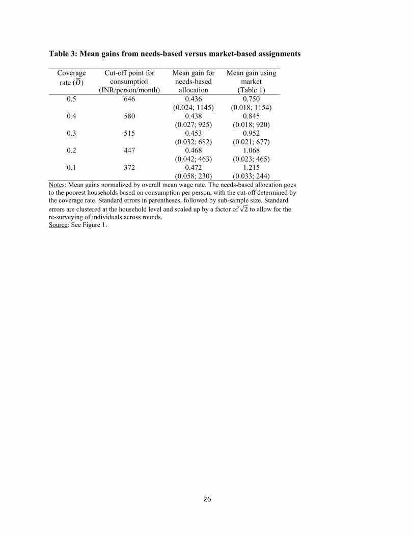
Turning to the “needs-based” counterfactual, the obvious criterion is household

consumption per person, as used for measuring poverty in India.13 Table 3 gives mean gains for

the same coverage rates, but now assigning from the lowest consumption per person upwards

until the coverage rate is met. (Table 3 also gives the required thresholds.) We see that the

“poverty-based” allocation achieves slightly higher mean gains than the actual mean (�̅�𝐺 =0.393),

but that it falls far short of the gains attainable with the “randomization plus resale” policy.

A common policy option to workfare is cash transfers. Starting from the same assignment

and with the same budget, tradeable BIKs can attain different welfare outcomes to cash transfers.

The interesting question in this context is how the policy option of allowing BIKs to be traded

alters the evaluative comparison of workfare versus cash transfers. Murgai et al. (2016) provide

revenue-neutral comparisons of MGNREGS in Bihar with hypothetical alternatives using cash

transfers. They show that, on taking account of forgone earnings and other costs in

implementation, the workfare scheme does no better than a (revenue-neutral) universal basic

income or transfers paid to those holding a ration card targeted to the poor, known as the “Below

Poverty Line” card. The outcomes for poverty are essentially the same across these options.

13 In practice this would probably be based on some form of proxy-means test, which would add extra errors of targeting; see, for example, Brown et al. (2019).

14

Since the comparison is a tie, the extent of the increase in mean gains found here when trade in

assignments is allowed suggests that this change in policy design would tilt the balance in favor

of the workfare scheme. Removing the current restrictions on transferability of assignments

would make this a more effective antipoverty policy than (revenue-neutral) cash transfers.

Heterogeneity in the gains: A key aspect of heterogeneity in this context is the extent of

poverty. We see from Figure 2 that the conditional mean gains tend to fall with higher household

consumption, although the (non-parametric) regression line is being pulled up at the bottom by a

few outliers. It is clear, however, that the mean gains from the market assignment are no lower

for those workers coming from households living below the median (Table 2, Columns (5) and

(7)). The potential gains are spread through the distribution of living standards.

Gender differences are also of interest. 29% of the sampled workers are women. The

overall mean gain is slightly lower for women. The relationship with household consumption is

similar by gender, though the tendency for the gains to fall as household consumption per person

rises tends to be less evident for women (Figure 2(b)). When one calculates mean gains

separately by gender (conditional on gains exceeding the market-clearing price), the differences

are small at all levels of coverage (Table 2).

The gender split in Table 2 assumes a common market for both genders. Instead, one

might split the market by gender (with trades only allowed among the same gender). This raises

the market-clearing price for men, and lowers it for women, while the aggregate gains remain

similar to Table 2. For example, at 𝐷𝐷� = 0.50, the equilibrium price rises to 0.31 for men and

falls to 0.18 for women, with mean gains of 0.760 and 0.724 respectively. The population

weighted mean gain across genders is 0.750 (Table 2).

4. Impediments to realizing the gains in practice

The evidence presented above is at least suggestive of large costs to poor people of

preventing trade in BIK assignments. However, there are reasons why the gains from allowing

trade may not be fully realized in practice. The reasons relate to market and institutional

impediments that also play a role in creating poverty in the first place. Thus, realizing the

potential gains from allowing tradeable assignments may require complementary policies.

15

Four main concerns can be identified. The first relates to credit-market imperfections,

such that poor potential beneficiaries simply cannot afford to purchase a BIK assignment.

Finding that the mean gains are no lower for poorer household does not, of course, imply that

poor households who did not get an initial assignment could afford to buy one. Given liquidity

constraints, the benefits may still be disproportionately captured by the relatively well off.

In support of this claim, Figure 3 gives the market price as a share of monthly

consumption for a family of five. The cost rises to a (clearly) prohibitive share of consumption

among poor families. Even the average shares for those living below the median are high; at a

coverage rate of 0.5, the purchase cost is a little over 20% of consumption; it rises to over 80% at

a coverage rate of 0.1. (Column 6 of Table 2 gives the share of monthly consumption for those

living below the median and the standard errors.) If the government insists on full payment of

the market price up-front this could be a prohibitively large share of consumption for poor

households.

One possible policy response is to introduce a “pay-as-you-go” option for those who do

not receive the program in the initial assignment but would benefit from purchasing it. Given that

this is a government-regulated market, the problem could be readily solved by introducing such

an option. Granted, one can anticipate resistance to such a step, as it can be interpreted as a

lowering of take-home wages for some. That concern would need to be weighed against the

potential benefits to poor workers in gaining access to the program.

Second, there will be scope for less liquidity-constrained, non-poor, people to participate

in the new market for BIKs. This is a concern, though it could also be addressed by policy design

features. In the context of explicitly targeted programs, one may want to maintain or even tighten

existing eligibility criteria. The norm in antipoverty and other social programs appears to be

under-coverage of those deemed eligible, with rationing among the set of eligible participants.14

While the results of this paper indicate large potential gains from allowing trade among those

eligible, there would be new risks in substantially expanding the set of those eligible since the

potential gains from trading assignments would attract more affluent participants not facing the

same liquidity constraints on participating in the market.

14 For an overview of evidence on this point see Ravallion (2017).

16

Another policy to address this second concern in the context of self-targeted programs

(such as the scheme studied here) is to introduce a minimum participation threshold. While the

self-targeting mechanism will tend to discourage participation by the well-off, creating the

market option could well impact selection into the program—attracting “speculators” and

middlemen who do not intend to work, but only re-sell their assignment if they get one.

However, one can avoid this by requiring a sufficiently long initial period of work before re-sale

is available as an option.

Third, there are impediments to the flow of knowledge in this setting. Dutta et al. (2014)

also surveyed participants’ knowledge about MGNREGS in Bihar. Most of the sample

(including over 90% of men) had heard of the scheme, but knowledge about the scheme’s rules

and provisions was poor, especially for women. The above calculations may overstate gains to

women relative to men.

Realizing the benefits from removing restrictions on trade requires that individual

participants are reasonably well-informed about their personal gains. Otherwise, there can be no

presumption that allowing resale will achieve an allocation that is any better than the status quo

or randomization on its own. Creating a market for BIK assignments would presumably change

the incentives for seeking and spreading information on the scheme. Even so, information

dissemination efforts would probably be needed, to complement a switch to tradeable

assignments in social programs.

There is evidence from the same setting that external intervention through “infotainment”

can enhance individual knowledge about this program and (hence) the individual gains.

Ravallion et al. (2015) report results from their RCT using an entertaining movie (produced for

this purpose) to teach people their rights and the rules and administrative procedures under the

scheme. The movie did enhance knowledge when assessed by a quiz given before and after

seeing the movie, and especially so for women. However, in studying the impacts of this RCT,

Alik-Lagrange and Ravallion (2019) find evidence of social frictions on information dispersal

within villages—frictions that disadvantage lower caste and poorer individuals.

The fourth concern is whether the administrative capacity will be present in poor places

to implement an efficient, largely corruption free, secondary market in BIK assignments. This is

no small matter. MGNREGA does have a quite sophisticated (public-access) web-based

17

information system, and it would seem plausible that the software to support a market for

assignments could also be developed, preferably integrated with the existing information

system.15 However, what actually happens on the ground could deviate appreciably from the

program’s formal operating rules. Dutta et al. (2014) identify a number of administrative

performance problems in poor areas of India that make it hard for the scheme studied here to

attain its potential impact on poverty even without allowing tradeable assignments. Ravallion

(2021) explains how rationing of jobs under MGNREGS could emerge in equilibrium given

local administrative costs in implementation and the scope for corruption by local leaders. These

features can also be thought of as examples of institutional failures that create poverty in the first

place. Of course, enhancing public administrative capacity is an important element of

development policy more broadly—a channel that is relevant to the efficacy of a wide range of

policies.

5. Conclusions

Governments often strive to prevent trade in assignments to antipoverty programs,

despite the lack of evidence on the welfare costs of doing so. Letting well-informed people trade

their assignments of benefits-in-kind can help programs attain the maximum aggregate gain with

perfect information even when the policy maker is ignorant of the individual gains. The

existence and relevance of private information is clearly one of the reasons why we know so

little about how much poor people might lose from such restrictions. This also has implications

for how we interpret evaluative evidence on the impacts of antipoverty programs.

Based on a theoretical model of a competitive market for assignments, the paper has

offered some evidence on the costs of preventing trade for a large antipoverty program in India.

The program aims to reduce poverty by providing jobs on labor-intensive public works projects.

A novel feature of the setting is that it is feasible to use surveys to measure individual pecuniary

gains from the jobs provided, even though this information is unlikely to be available for

implementing a scheme of transferable in-kind benefits. The surveyed workers were asked about

both actual wages received and labor-market options at the time. Using these data, the paper has

15 The existing information system does not record the extent of rationing under the scheme. Under the scheme’s rules, the state government is responsible for paying an unemployment allowance if work cannot be found. This gives the state government a strong incentive to report that all requests for work were honored. That is inconsistent with what has been observed based on surveys (Dutta et al. 2012, 2014; Desai et al. 2015).

18

simulated various stylized schemes of randomized assignment with resale, at different levels of

coverage, and studied the gains from such a policy, including their incidence by household levels

of living and the gender of workers.

The calculations indicate that there are large unexploited gains to poor people from

allowing trade in work assignments. A competitive market for tradeable assignments would

generate aggregate gains that are around 2 to 3 times the current mean gains to these (mostly

very poor) families. It would also have greater impact (by a similar magnitude in terms of mean

gains) than an allocation without re-sale options targeted to workers from consumption-poor

families. Allowing the assignments to be tradeable in this setting can also make workfare more

effective against poverty than (budget-neutral) cash transfers.

The results do not suggest that the gains from the market-based assignment would tend to

favor more affluent families; the mean gains were very similar between the poorest half in terms

of household consumption per person as for the rest. The simulated allocations with tradeable

assignments imply a tendency for somewhat larger gains among poorer households, not the

opposite. Gains are similar between male and female workers.

The paper has also pointed to some likely impediments to fully realizing these gains in

practice, including credit market failures, capture by non-poor speculators, and imperfect

information. There are complementary policies that may well be needed to realize the gains to

poor people from allowing tradeable assignments. A “pay-as-you-go” option could help address

liquidity constraints stemming from credit market imperfections. Eligibility criteria and

minimum participation requirements (to encourage self-targeting) could help dissuade non-poor

speculators and middlemen from entering the market. And information campaigns are clearly

desirable, and not so hard to do. Limitations on local-level administrative capacity and the

(related) scope for corruption also warn for caution. The same features impede many other

aspects of economic development.

As is often the case, success in one policy effort—in this case assuring that the benefits to

poor people of an antipoverty program are fully realized—may require success on multiple

fronts.

19

References

Alik Lagrange, Arthur, and Martin Ravallion, 2018. “Workfare versus Transfers in Rural India,”

World Development 112: 244-258.

Alik Lagrange, Arthur, and Martin Ravallion, 2019. “Estimating Within-Group Spillover Effects

Using a Cluster Randomization: Knowledge Diffusion in Rural India,” Journal of

Applied Econometrics 34: 110-128.

Besley, Timothy, and Stephen Coate, 1992, “Workfare vs. Welfare: Incentive Arguments for

Work Requirements in Poverty Alleviation Programs,” American Economic Review

82(1): 249–61.

Brown, Caitlin, Martin Ravallion and Dominique van de Walle, 2018, “A Poor Means Test?

Econometric Targeting in Africa,” Journal of Development Economics 134: 109-124.

Che, Yeon-Koo, Ian Gale and Jinwoo Kim, 2013, “Assigning Resources to Budget-Constrained

Agents,” Review of Economic Studies 80(1): 73-107.

Currie, Janet, and Firouz Gahvari, 2008, “Transfers in Cash and In-Kind: Theory Meets the

Data,” Journal of Economic Literature 46(2): 333-383.

Datt, Gaurav, and Martin Ravallion, 1994, “Transfer Benefits from Public-Works Employment,”

Economic Journal 104: 1346-1369.

Desai, Sonalde, Prem Vashishtha and Omkar Joshi (2015), Mahatma Gandhi National Rural

Employment Guarantee Act: A Catalyst for Rural Transformation, New Delhi: National

Council of Applied Economic Research.

Dutta, Puja, Rinku Murgai, Martin Ravallion and Dominique van de Walle, 2012, “Does India’s

Employment Guarantee Scheme Guarantee Employment?” Economic and Political

Weekly 48 (April 21): 55-64.

Dutta, Puja, Rinku Murgai, Martin Ravallion and Dominique van de Walle, 2014, Right-to-

Work? Assessing India’s Employment Guarantee Scheme in Bihar. World Bank.

Heckman, James, Serio Urzua and Edward Vytlacil, 2006, “Understanding Instrumental

Variables in Models with Essential Heterogeneity,” Review of Economics and Statistics

88(3): 389-432.

Himanshu, 2019, “Inequality in India: Review of Levels and Trends,” WIDER WP 2019/42.

Moffitt, Robert, 2006, “Welfare Work Requirements with Paternalistic Government

Preferences,” Economic Journal 116(515): F441-F458.

20

Murgai, Rinku, Martin Ravallion and Dominique van de Walle (2016), “Is Workfare Cost

Effective against Poverty in a Poor Labor-Surplus Economy?,” World Bank Economic

Review 30(3):413-445.

Narita, Yusuke, 2018. “Toward an Ethical Experiment,” Cowles Foundation Discussion Paper

No. 2127, Yale University.

Ravallion, Martin, 2017, Interventions against Poverty in Poor Places, 20th Annual WIDER

Lecture, World Institute of Development Economics, Helsinki.

Ravallion, Martin, 2020, “Is a Decentralized Right-to-Work Policy Feasible?” Development,

Distribution, and Markets, Kaushik Basu, Kenneth Kletzer, Sudipto Mundle and Eric

Verhoogen (eds), New Delhi: Oxford University Press.

Ravallion, Martin, Gaurav Datt, and Shubham Chaudhuri, 1993, “Does Maharashtra’s

‘Employment Guarantee Scheme’ Guarantee Employment? Effects of the 1988 Wage

Increase,” Economic Development and Cultural Change 41: 251–75.

Ravallion, Martin, Dominique van de Walle, Rinku Murgai and Puja Dutta, 2015, “Empowering

Poor People through Public Information? Lessons from a Movie in Rural India,” Journal

of Public Economics 132: 13-22.

Sah, Raaj Kumar, 1987, “Queues, Rations, and Market: Comparisons of Outcomes for the Poor

and the Rich,” American Economic Review 77(1): 69-77.

Weitzman, Martin, 1977, “Is the Price System or Rationing More Effective in Getting a

Commodity to Those Who Need it Most?” Bell Journal of Economics 8(2): 517-524.

21

Figure 1: Conditional mean gains (𝐸𝐸�(𝐺𝐺𝑖𝑖|𝐺𝐺𝑖𝑖 > 𝑋𝑋))

0.0

0.2

0.4

0.6

0.8

1.0

1.2

1.4

0.0 0.1 0.2 0.3 0.4 0.5 0.6 0.7 0.8 0.9 1.0 1.1 1.2X

Mea

n ga

in (n

orm

alize

d by

ave

rage

wag

e ra

te)

Conditional mean

Mean

X

Mea

n ga

in (n

orm

alize

d by

ave

rage

wag

e ra

te)

Conditional mean

Mean

Note: Gain from employment in the National Rural Employment Guarantee Scheme in Bihar, India. The gain is normalized by the overall mean wage rate (84.28 INR per day). Lower and upper bounds of the 95% confidence intervals. Standard errors are clustered at the household level and scaled up by a factor of √2 to allow for the re-surveying of individuals across rounds. Source: Author’s calculations from the survey data collected in two rounds, 2009-10, by a team including the author and documented in Dutta et al. (2014). N=2307 after deleting 17 implausibly high outliers (exceeding 400 INR per day).

22

Figure 2: Gains plotted against household consumption per person

(a) All workers

0.0

0.5

1.0

1.5

2.0

2.5

3.0

3.5

4.0

5.0 5.5 6.0 6.5 7.0 7.5 8.0 8.5 9.0 9.5

Household consumption per person (log scale)

Gai

n (n

orm

alize

d by

mea

n w

age

rate

)

Household consumption per person (log scale)

Gai

n (n

orm

alize

d by

mea

n w

age

rate

)

(b) Split by gender

0.0

0.4

0.8

1.2

1.6

2.0

2.4

2.8

3.2

3.6

5.0 5.5 6.0 6.5 7.0 7.5 8.0 8.5 9.0 9.5

Household consumption per person (log scale)

Male workersFemale workers

MaleFemale

Household consumption per person (log scale)

MaleFemale

Note: See Figure 1. Nearest neighbor smoothed scatter plot. Source: See Figure 1.

23

Figure 3: Market price of assignments as a share of household consumption

0.0

0.4

0.8

1.2

1.6

2.0

5.0 5.5 6.0 6.5 7.0 7.5 8.0 8.5 9.0 9.5

Household consumption per person (log scale)

0.10.20.30.40.5

Coverage rate=

Shar

e of

hou

seho

ld co

nsum

ptio

n

Household consumption per person (log scale)

Coverage rate=

Shar

e of

hou

seho

ld co

nsum

ptio

n

Note: Share of consumption calculated for a household of five people with one person selling an assignment for 20 days per month. Nearest neighbor smoothed scatter plots. Source: See Figure 1.

24

Table 1: Summary statistics on monetary gains from jobs on a workfare scheme in Bihar, India

Sample mean

Standard error

N

Gain 0.393 0.017 2307 Gain for workers in households with below median consumption per person

0.436 0.024 1150

Gain for workers in households with above median consumption per person

0.350 0.031 1151

Gain for female workers 0.363 0.031 669 Gain for male workers 0.406 0.020 1638 Gain for female workers in household with below median consumption per person

0.435 0.047 315

Gain for male workers in household with below median consumption per person

0.437 0.027 835

Gain for female workers in household with above median consumption per person

0.299 0.037 352

Gain for male workers in household with above median consumption per person

0.373 0.028 799

Notes: Mean gains (wage rate less forgone earnings) normalized by overall mean wage rate. 17 extreme values for the gains (exceeding 400% of mean wage rate) are dropped. Standard errors are clustered at the household level and scaled up by a factor of √2 to allow for the re-surveying of individuals across rounds.

25

Table 2: Mean gains from competitively tradeable assignments

(1) (2) (3) (4) (5) (6) (7) (8) (9) Coverage rate (𝐷𝐷�)

Market-clearing price (𝑃𝑃)

Pop. share

trading

Mean gain for treated

(𝐸𝐸�(𝐺𝐺𝑖𝑖|𝐺𝐺𝑖𝑖 > 𝑃𝑃))

Mean gain for those below

median consumption

Share of consumption for below median

household

Mean gain for those above

median consumption

Mean gain for female

workers

Mean gain for male workers

0.5 0.28 0.25 0.750 (0.018; 1154)

0.736 (0.024; 654)

0.217 (0.004; 654)

0.767 (0.028; 497)

0.757 (0.030; 312)

0.748 (0.030; 842)

0.4 0.47 0.24 0.845 (0.018; 920)

0.826 (0.024; 522)

0.363 (0.007; 522)

0.869 (0.030; 395)

0.827 (0.030; 262)

0.852 (0.023; 658)

0.3 0.60 0.21 0.952 (0.021; 677)

0.944 (0.027; 367)

0.463 (0.011; 367)

0.963 (0.030; 307)

0.931 (0.028; 190)

0.961 (0.025 487)

0.2 0.81 0.16 1.068 (0.023; 465)

1.059 (0.030; 249)

0.642 (0.020; 249)

1.078 (0.033; 214)

1.043 (0.025;129)

1.078 (0.030; 336)

0.1 1.05 0.09 1.215 (0.033; 244)

1.217 (0.042; 126)

0.834 (0.038; 126)

1.214 (0.047; 117)

1.188 (0.018; 63)

1.225 (0.044; 181)

Notes: Mean gains normalized by overall mean wage rate. The status quo mean is 0.393 (s.e.=0.017). Equilibrium prices calculated numerically to nearest second decimal place. Share of consumption (column 6) calculated for household of five people with one person selling an assignment for 20 days per month. Median consumption per person=INR 647 per month. Standard errors in parentheses, followed by sub-sample size. Standard errors are clustered at the household level and scaled up by a factor of √2 to allow for the re-surveying of individuals across rounds. Source: See Figure 1.

26

Table 3: Mean gains from needs-based versus market-based assignments

Coverage rate (𝐷𝐷�)

Cut-off point for consumption

(INR/person/month)

Mean gain for needs-based allocation

Mean gain using market

(Table 1) 0.5 646 0.436

(0.024; 1145) 0.750

(0.018; 1154) 0.4 580 0.438

(0.027; 925) 0.845

(0.018; 920) 0.3 515 0.453

(0.032; 682) 0.952

(0.021; 677) 0.2 447 0.468

(0.042; 463) 1.068

(0.023; 465) 0.1 372 0.472

(0.058; 230) 1.215

(0.033; 244) Notes: Mean gains normalized by overall mean wage rate. The needs-based allocation goes to the poorest households based on consumption per person, with the cut-off determined by the coverage rate. Standard errors in parentheses, followed by sub-sample size. Standard errors are clustered at the household level and scaled up by a factor of √2 to allow for the re-surveying of individuals across rounds. Source: See Figure 1.