Welfare Gains from Foreign Direct Investment throughTechnology Transfer to Local Suppliers∗

Garrick Blalock† Paul J. Gertler‡

May 15, 2005

Abstract

We hypothesize that multinational firms operating in emerging markets transfertechnology to local suppliers to increase their productivity and lower input prices.To avoid hold-up by any single supplier, the foreign firm must make the technologywidely available. This technology diffusion induces entry and more competition whichlowers prices in the supply market. As a result, not just the foreign-owned firm,but all firms downstream of that supply market obtain lower prices. We test thishypothesis using a panel dataset of Indonesian manufacturing establishments. We findstrong evidence of productivity gains, greater competition, and lower prices amonglocal firms in markets that supply foreign entrants. The technology transfer is Paretoimproving—value added and output increase for firms in both the supplier and buyersectors. Further, the technology transfer generates an externality that benefits buyersin other sectors downstream from the supply sector as well. This externality mayprovide a justification for policy intervention to encourage foreign investment.

Keywords:Foreign Direct Investment, Technology Transfer, Productivity, Supply ChainJ.E.L. codes: F23, O14, O12, H41

∗We are indebted to Indra Surbakti, Fitria Fitrani, Kai Kaiser, and Jack Molyneaux for their assistancein compiling the data. We received helpful advice from David I. Levine, David C. Mowery, Pranab Bardhan,Ann Harrison, Mary Amati, Nina Pavcnik, James E. Blalock, Haryo Aswicahyono, and Thee Kian Wei. Wethank the Institute of Business and Economic Research (IBER) and Management of Technology (MOT)program, both at the University of California, Berkeley, for their generous financial support. We receivedhelpful comments from seminar participants at The Pennsylvania State University and the London Schoolof Economics and Political Science. Finally, we are grateful to the factory managers in Indonesia who kindlyparticipated in interviews.

†Corresponding author. Cornell University, Department of Applied Economics and Management, 346Warren Hall, Ithaca, NY 14853 USA. +1 (607) 255-0307, +1 (607) 255-9984 fax.garrick.blalock@cornell.edu

‡University of California, Berkeley, Haas School of Business, and NBER, gertler@haas.berkeley.edu

1

1 Introduction

Many countries try to attract foreign direct investment (FDI) with costly public programs,

such as tax holidays, subsidized industrial infrastructure, and duty exemptions. Is this

enthusiasm for FDI warranted? In this paper, we investigate the hypothesis that multina-

tional firms transfer technology to their domestic suppliers and that this transfer generates

greater competition and lower prices that benefit the entire economy. If true, the effect on

competition may justify public encouragement of FDI.

Recently, a number of authors have argued that that multinationals may deliberately

transfer technology to local suppliers as part of a strategy to build efficient supply chains

for overseas operations (Pack and Saggi 2001; Blalock 2002; Javorcik 2004). By transferring

technology to local suppliers, the downstream multinationals lower the cost of non-labor

inputs. This cost-reduction motive implies that multinationals transfer technology to sup-

pliers because it confers a private benefit to them. However, unless there is an additional

social benefit, there is no case for public subsidies to stimulate technology transfers from

multinationals.

How might social benefits develop? The primary motivation for multinationals to transfer

technology to suppliers is to enable higher quality inputs at lower prices. One problem with

this strategy is that if the enabling technology is transferred to only one upstream vendor,

then the multinational is vulnerable to hold-up. To mitigate hold-up risk, the multinational

could diffuse the technology widely—either by direct transfer to additional firms or by en-

couraging spillover from the original recipient. The wide diffusion of the technology would

then encourage entry in the supplier market, thereby increasing competition and lowering

prices. However, the multinational cannot prevent the upstream suppliers from also selling

to others in downstream markets. The lower input prices may induce entry and therefore

more competition in downstream markets, which lowers prices and increases output. Pack

and Saggi (2001) show that theoretically, as long as there is not too much entry, profits will

rise in both the downstream and upstream markets. If so, then the new surplus generated

2

from increased productivity and the deadweight loss reduced from increased competition will

be split between consumers and producers in a Pareto-improving distribution.

In this paper we test the hypotheses that FDI lead to a Pareto superior increase in welfare

via these mechanisms. Specifically, we examine whether there were transfers of technology

along the supply chain, whether the technology transfer leads to increased competition, and

whether the increased competition induced welfare improvements in terms of lower prices,

greater production, and higher profits in both the supply market and in sectors downstream of

the supply market. Our chief contribution is to establish and quantify the welfare enhancing

externalities of vertical technology transfer.

The analysis is in two parts. The first part measures the effect of FDI on local supplier

productivity by estimating a production function using a rich panel dataset on local- and

foreign-owned Indonesian manufacturing establishments. In a number of industries, the

realized productivity gain is more than two percent. The second part of the paper examines

the market and welfare effects of technology diffusion from FDI. We find that downstream

FDI increases the output and value added of upstream firms, and decreases prices and market

concentration of upstream markets. We also find increased output and value added among

downstream firms, and decreased prices and market concentration in markets downstream of

markets supplying multinationals. In sum, our findings suggest several welfare effects—i.e.,

benefits for consumers in terms of lower prices and for firms in the form of greater value

added—transmitted both up and down the supply chain from the adoption of technology

brought with FDI.

2 Conceptual Framework

Policymakers often cite technology diffusion to host country firms as a benefit of foreign

direct investment (FDI). This belief proliferates in part because of impressive claims of

technological development from FDI, such as those of the World Bank (1993, p. 1), which

3

writes that “[FDI] brings with it considerable benefits: technology transfer, management

know-how, and export marketing access. Many developing countries will need to be more

effective in attracting FDI flows if they are to close the technology gap with high-income

countries, upgrade managerial skills, and develop their export markets.”

The proponents offer three explanations for how technology spillovers from multinationals

to domestic competitors. First, the local firm may be able to learn simply by observing and

imitating the multinationals. Second, employees may leave multinationals to create or join

local firms. Third, multinational investment may encourage the entry of international trade

brokers, accounting firms, consultant companies, and other professional services, which then

may become available to local firms as well.

However, a number of recent empirical studies, which find mixed evidence of technology

transfer from FDI, have prompted many observers to question its existence. Rodrik (1999,

p. 37), in a summary of the evidence, comments, “today’s policy literature is filled with

extravagant claims about positive spillovers from FDI, [but] the hard evidence is sobering.”

The studies to which Rodrik refers ask if local competitors benefit from a positive externality,

or “technology spillover,” generated by multinational entry in the same industry.1

Indeed, it is hard to believe that such horizontal spillovers are likely. First, the tech-

nology gap between foreign and domestic firms may often be wide. Local firms may lack

the absorptive capacity needed to recognize and adopt the new technology. Similarly, the

degree to which foreign and domestic firms actually compete in the same market will also

vary. Domestic firms may produce for the local market while multinationals produce for

export. Because of differences in quality and other attributes, exported and domestically

consumed goods may entail different production methods which reduce the potential for

technology transfer. Second, multinationals may enact measures to minimize technology

leakage to local competitors. Multinationals with non-protectable technology may not enter

1Examples of empirical papers measuring technology spillovers include Blomstrom and Wolff 1994, Had-dad and Harrison 1993, Kokko 1994, Aitken and Harrison 1999, Aitken and Harrison 1999, and Haskel,Pereira, and Slaughter 2002. See Moran 2001 and Keller 2004 for excellent surveys of the evidence.

4

the market at all if they rely on a technological advantage to sustain rents. Further, foreign

firms typically pay managers higher wages to discourage technology leakage through former

employees. In fact, because of the higher wages, foreign firms may instigate a “brain drain”

that lures the most capable managers away from domestic firms.

In contrast, technological benefits to local firms through vertical linkages are much more

likely since the multinational has incentives to provide technology to suppliers. Vertical

technology transfer could occur through both backward (from buyer to supplier) and forward

(from supplier to buyer) linkages. Because most multinationals in Indonesia are export-

oriented and generally do not supply Indonesian customers, we focus here on technology

transfer through backward linkages. That is, we examine the effect of downstream FDI on

the performance of local suppliers.

Two arguments suggest that supply chains may be a conduit for technology transfer.

First, whereas multinationals seek to minimize technology leakage to competitors, they have

incentives to improve the productivity of their suppliers through training, quality control,

and inventory management, for example. To reduce dependency on a single supplier, the

multinational may establish such relationships with multiple vendors, which benefits all firms

which purchase these vendors’ output. Second, while the technology gap between foreign and

domestic producers may limit within-sector technology transfer, multinationals likely procure

inputs requiring less sophisticated production techniques for which the gap is narrower.

Evidence of technology transfer through vertical supply chains is well documented in case

studies. For example, Kenney and Florida 1993 and Macduffie and Helper 1997 provide a

rich description of technology transfer to U.S. parts suppliers following the entry of Japanese

automobile makers. Until recently, empirical analysis, however, is generally limited to small

samples, such as that by Lall (1980), which documents technology transfer from foreign firms

through backward linkages in the Indian trucking industry. Blalock 2002 finds evidence of

technology transfer through the supply chain in production function estimates in Indonesia,

and Javorcik 2004 finds similar results in Lithuania.

5

Multinationals transfer technology to suppliers to reduce input costs and increase quality.

However, if the multinational aids only a single supplier, the supplier can play hold-up and

capture all of the rents from its increased productivity. In this case, the multinational would

not benefit from the technology transfer. The multinational could overcome this vulnera-

bility, however, by distributing the technology widely to multiple suppliers and potential

entrants. This would create multiple sources of superior supply and would encourage en-

try (competition) that would lower prices. Total surplus rises because the new technology

increases productivity and because the deadweight from imperfect competition falls. The

downstream multinational captures some of the rent because the prices it pays for supplies

have fallen. However, if there is not too much entry, the suppliers may also capture some of

the rent in terms of profits resulting from increased productivity and sales (Pack and Saggi

2001).

Although the multinational has an incentive to aid many suppliers, doing so may inad-

vertently aid competitors if the more productive supply base is a non-excludable benefit.

That is to say that the multinational cannot prevent its now more productive suppliers from

also selling to the multinational’s rivals at lower prices. The lower supply prices may induce

entry and increase competition so that prices fall in the downstream markets as well. In sum,

these actions increase surplus by lowering costs of production and by reducing deadweight

loss from imperfect competition. Moreover, the lower supply prices not only increase surplus

in the multinational’s market, but in all of the markets to which the suppliers sell.

In a developing country setting, where generally export-oriented foreign firms are more

productive than domestic firms and seldom compete with domestic makers anyway, aiding

local buyers may not concern multinationals. However, foreign firms may be concerned that

their investment in the local supply chain will eventually benefit later foreign entrants. Given

this possibility, one might think that foreign firms would be reluctant to transfer technology

to suppliers.

The structural model in Pack and Saggi 2001 shows that, provided new competition is

6

not too great, the benefits of a competitive supply base to the multinational buyer outweigh

the rents lost to free-loading rivals. Perhaps surprisingly, technology diffusion and leakage

to other local suppliers can also benefit the initial local recipient. In the case of a single

supplier and just one buyer with some market power, both parties set prices above marginal

cost—the “double marginalization problem.” If technology diffusion to other upstream firms

allows more capable suppliers to enter, then one would expect market concentration and

input prices to fall. Further, given the benefit of lower-priced inputs, firms downstream of

that upstream sector will lower prices and increase output, and new firm entry may occur.

The stronger demand downstream would, in turn, prompt higher output upstream that

would help the initial technology recipient. Lower prices and greater volume clearly generate

a surplus for consumers. Pack and Saggi 2001 note that in some cases, firms may be able

to capture some of the surplus also because the benefits of lower input prices and higher

volume outweigh the costs of greater competition. Here, we would expect to see firm value

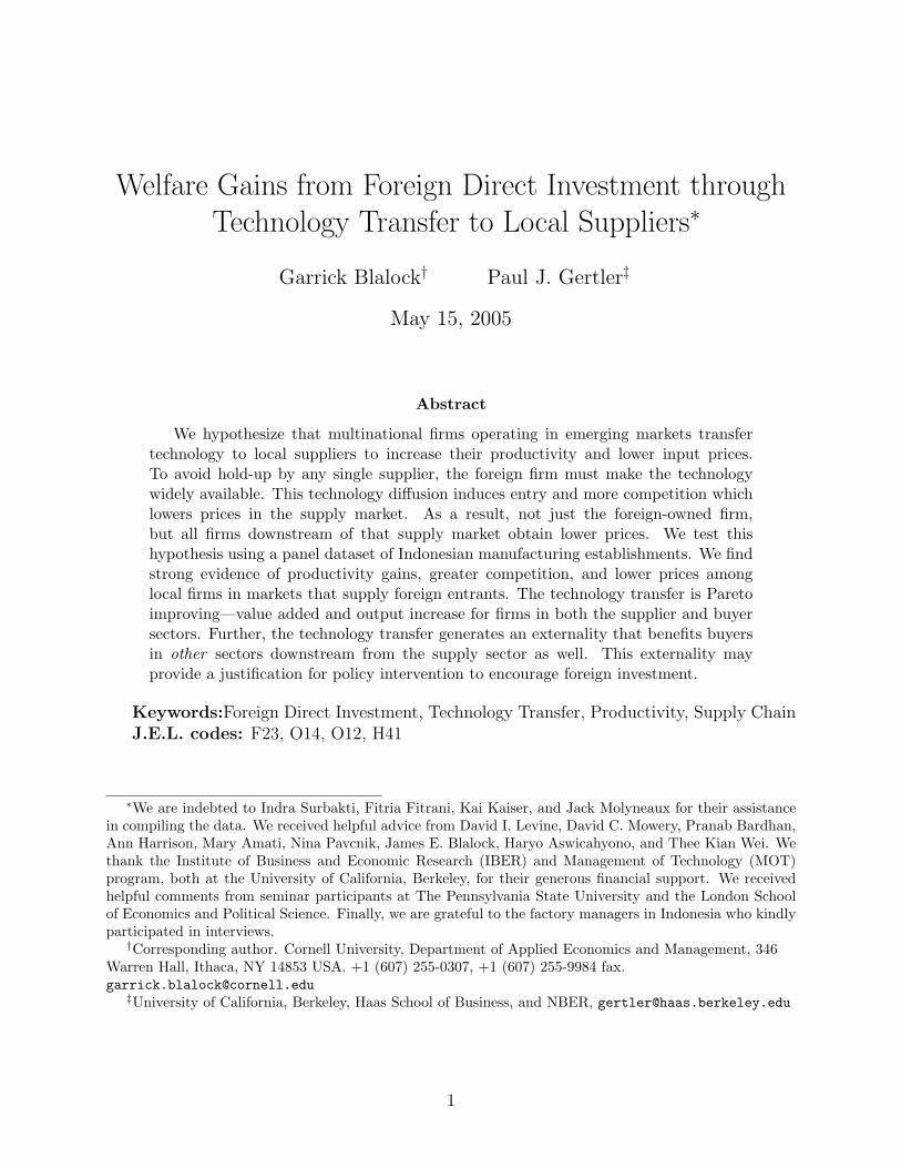
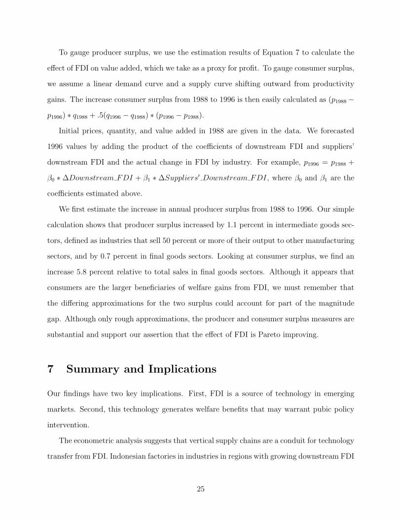
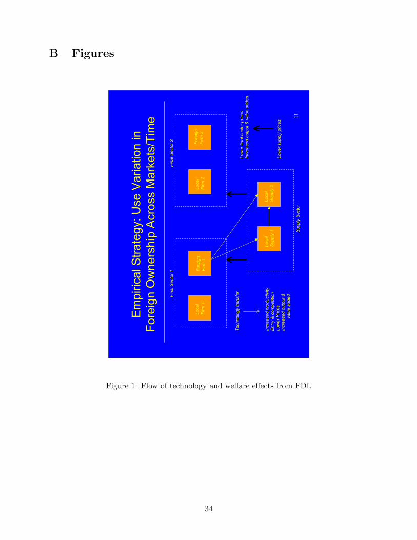
added—a proxy for profitability—rise.2 Figure 1 illustrates the total effect of FDI.

If the above argument is true, then technology transfer to suppliers is in multinationals’

interest, but the benefits accrue widely to all sectors and consumers not only through im-

proved productivity, but also through increased competition resulting in lower deadweight

loss. Hence, technology transfer induces a Pareto improvement in welfare. However, a

multinational might not take into account the social benefits of increased competition, and

therefore may transfer too little technology. In this case, it would be socially optimal to

facilitate the transfer of technology from multinationals to local suppliers.

Although the specific mechanisms for technology transfer described above are typically

unobservable in the data, one can identify technology transfer indirectly by otherwise unex-

plained productivity gains. If vertical supply chains are a conduit for technology transfer,

then one would expect, ceteris paribus, that local firms in industries and regions with grow-

ing levels of downstream FDI would show greater productivity growth than other local firms.

2We define value added as revenue minus wages and the cost of materials and energy. This is similar toEBITDA (Earnings before interest, taxes, depreciation, and amortization, a common proxy for profitability.

7

Further, one would expect to see lower concentration, lower prices, higher output, and more

value added in these beneficiary sectors, as well as in sectors downstream of them. The

methodology for testing the productivity effects is described in Section 5, and the methodol-

ogy for testing the market and welfare effects is described in Section 6. Both are preceded by

some background on Indonesian manufacturing and a description of the data in the following

two sections.

3 Indonesian Manufacturing and Foreign Investment

Policy

Indonesia’s manufacturing sector is an attractive setting for research on FDI and technology

transfer for several reasons. First, with the fourth largest population in the world and

thousands of islands stretching over three time zones, the country has abundant labor and

natural resources to support a large sample of manufacturing facilities in a wide variety of

industries. Further, the country’s size and resources support a full supply chain, from raw

materials to intermediate and final goods, and both export and domestic markets. Second,

rapid and localized industrialization provides variance in manufacturing activity in both time

and geography. Third, the country’s widespread island archipelago geography and generally

poor transportation infrastructure create a number of local markets, each of which can

support independent supply chains. Fourth, a number of institutional reforms of investment

law have dramatically increased the amount of FDI and export activity in recent years. In

particular, the nature and timing of these reforms provide exogenous variation in FDI by

region, industry, and time that will be exploited in the econometric identification. Last,

Indonesian government agencies employ a number of well trained statisticians who have

collected exceptionally rich manufacturing data for a developing country.

The Indonesian economy and the manufacturing sector grew dramatically from the late

8

1970’s until the recent financial crisis.3 Indonesia enjoyed an average annual GDP growth rate

of 6-7 percent and much of this growth was driven by manufacturing, which expanded from

11 percent of GDP in 1980 to 25 percent in 1995 (Nasution 1995). Government initiatives

to reduce dependency on oil and gas revenue in the mid-1980’s, principally liberalization of

financial markets and foreign exchange, a shift from an import-substitution regime to export

promotion, currency devaluation, and relaxation of foreign investment laws, facilitated the

large increase in manufacturing output (Goeltom 1995).

Over the past 40 years, government regulation has shifted dramatically from a policy

antagonistic to FDI to a policy actively encouraging it (Wie 1994; Hill 1988; Pangestu 1996).

Following independence from the Netherlands in 1945, the Sukarno government nationalized

many of the former Dutch manufacturing enterprises. Weak property rights and socialist

rhetoric kept foreign investment at a trickle throughout the 1950’s and 1960’s.

Gradual reforms began in 1967 as part of the “New Order” economic regime of Suharto.

The reforms allowed investment in most sectors, but still required substantial minimum lev-

els of initial and long-term Indonesian ownership in new ventures. Following the collapse of

oil prices in the mid-1980’s, the government began to seek outside investment more actively.

From 1986 to 1994, it introduced a number of exemptions to the restrictions on foreign

investment. The exemptions were targeted to multinationals investing in particular loca-

tions, notably a bonded zone on the island of Batam (only 20 kilometers from Singapore),

government sponsored industrial parks, and undeveloped provinces of east Indonesia. The

new policy also granted exemptions to investment in capital-intensive, technology-intensive,

and export-oriented sectors. Moreover, the reforms reduced or eliminated import tariffs for

certain capital goods and for materials that would be assembled and exported.

Finally, in 1994 the government lifted nearly all equity restrictions on foreign investment.

Multinationals in most sectors were allowed to establish and maintain in perpetuity oper-

ations with 100 percent equity. In a handful of sectors deemed strategically important, a

3Hill (1988) and Pangestu and Sato (1997) provide detailed histories of Indonesian manufacturing fromthe colonial period to the present.

9

nominal 5 percent Indonesian holding was required with no further requirement to divest.

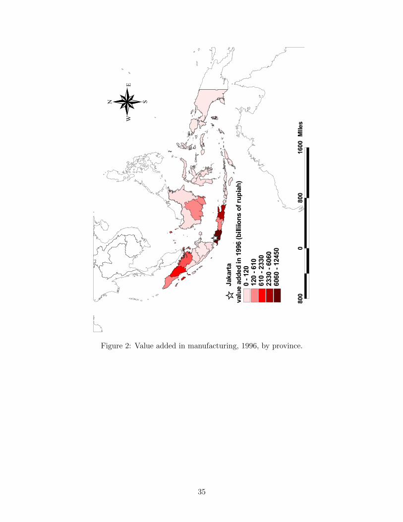
The reforms have been accompanied by large increases in both the absolute and the

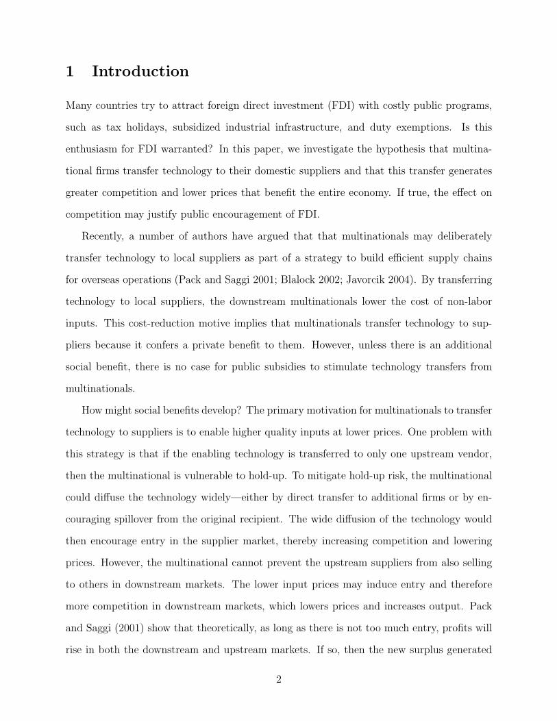
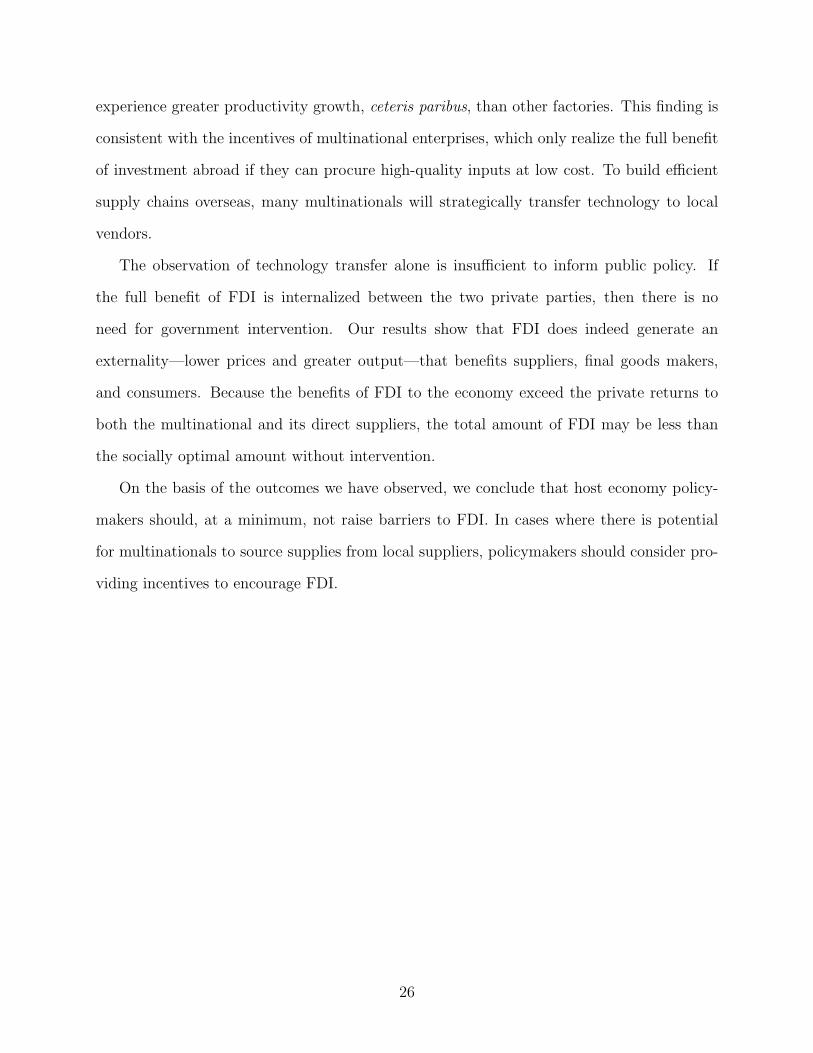
relative value of foreign production in Indonesian manufacturing. Figure 2 shows the real

value added by foreign firms in 1996 by province. The map indicates significant regional

variation and shows the absolute level of foreign output to be very large. For example, the

value added by multinational manufacturing in the province of Riau (the closest province to

Singapore and home to the Batam bonded zone) is 2,335 billion rupiah, or about 10 percent

of the province GDP. Large foreign investment from 1988 to 1996 in chemicals, plastics,

electronics assembly, textiles, garments, and footwear dramatically increased the foreign

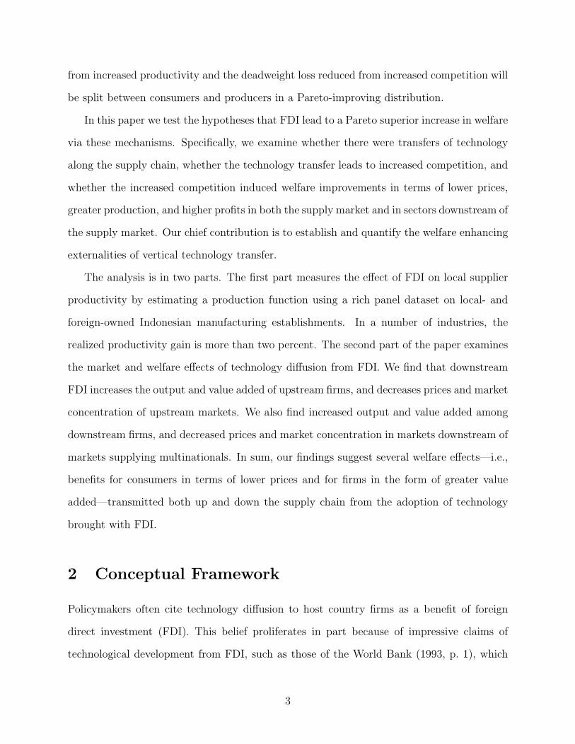
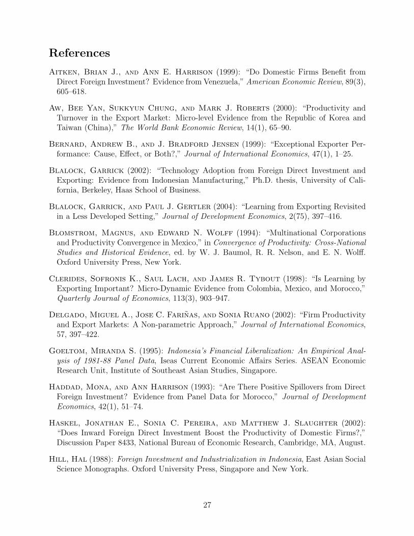
output in many areas. Figure 3 shows the foreign share of manufacturing value added in

1988 and 1996, respectively, by province. In many regions the foreign share of value added

increased dramatically from 1988 to 1996 and accounted for more than half of the total in

1996.

4 Data

The analysis is based on data from the Republic of Indonesia’s Budan Pusat Statistik (BPS),

the Central Bureau of Statistics.4 The primary data are taken from an annual survey of

manufacturing establishments with more than 20 employees conducted by Biro Statistik

Industri, the Industrial Statistics Division of BPS. Additional data include the input-output

table and several input and output price deflators.

The principal dataset is the Survei Tahunan Perusahaan Industri Pengolahan (SI), the

Annual Manufacturing Survey conducted by the Industrial Statistics Division of BPS. The SI

dataset is designed to be a complete annual enumeration of all manufacturing establishments

with 20 or more employees from 1975 onward. Depending on the year, the SI includes up

to 160 variables covering industrial classification (5-digit ISIC), ownership (public, private,

4We identify names in Bahasa Indonesia, the language of most government publications, with italics.Subsequently, we use the English equivalent or the acronym.

10

foreign), status of incorporation, assets, asset changes, electricity, fuels, income, output,

expenses, investment, labor (head count, education, wages), raw material use, machinery,

and other specialized questions.

BPS submits a questionnaire annually to all registered manufacturing establishments,

and field agents attempt to visit each non-respondent to either encourage compliance or

confirm that the establishment has ceased operation.5 Because field office budgets are partly

determined by the number of reporting establishments, agents have some incentive to identify

and register new plants. In recent years, over 20,000 factories have been surveyed annually.

Government laws guarantee that the collected information will only be used for statistical

purposes. However, several BPS officials commented that some establishments intentionally

misreport financial information out of concern that tax authorities or competitors may gain

access to the data. Because the fixed-effect analysis admits only within-factory variation on

a logarithmic scale, errors of under- or over-reporting will not bias the results provided that

each factory consistently misreports over time. Further, even if the degree of misreporting

for a factory varies over time, the results are unbiased provided the misreporting is not

correlated with other factory attributes in the right-hand-side of the regression.

The analysis here starts from 1988, the first year data on fixed assets are available. To

avoid measurement error in price and other uncertainties introduced by the 1997-1998 Asian

financial crisis, the last year of analysis is 1996. The key variables are described in Appendix

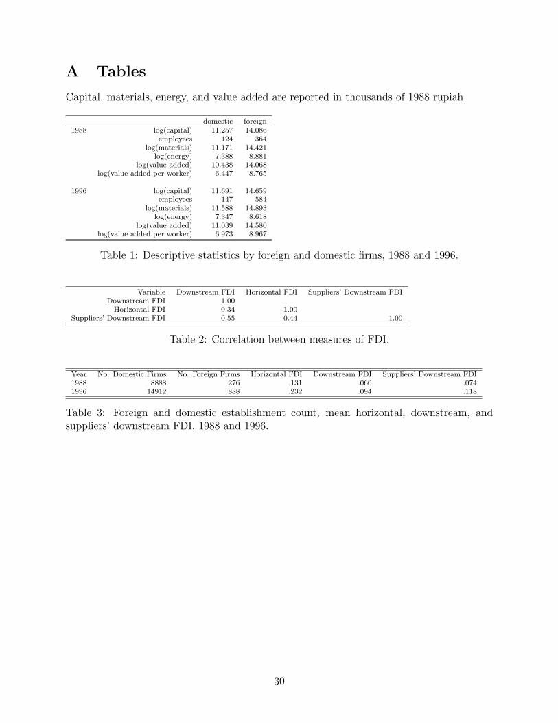
C and summarized for 1988 and 1996 in Table 1. On average, foreign factories are bigger

(as measured by value added, employees, and capital), more capital intensive (as measured

by capital per employee), more productive (as measured by value added per employee), and

more export-oriented (as measured by percentage of production exported). Table 3 shows

the sample count, which grew from 8,888 to 14,912 and from 276 to 888 for domestic and

5Because some firms may have more than one factory, we henceforth refer to each observation as anestablishment, plant, or factory. BPS also submits a different questionnaire to the head office of every firmwith more than one factory. Although these data were not available for this study, early analysis by BPSsuggests that less than 5 percent of factories belong to multi-factory firms. We thus generalize our resultsto firms in our discussion.

11

foreign factories respectively.

We derived inter-industry supply chains using input-output (IO) tables published by

BPS in 1990 and 1995. The tables show the value added of goods and services produced by

economic sector and how this value is distributed to other economic sectors. The IO tables

divide manufacturing activity into 89 sectors, and BPS provides concordance tables linking

the 1990 and 1995 IO codes to 5-digit ISIC codes as described in Appendix D.

We deflated output, materials, energy, and capital to express values in real terms. Ap-

pendix D describes the deflator calculation in detail.

Not surprisingly, particularly in a developing country environment, there is a high level of

non-reporting and obvious erroneous responses to many of the survey questions, particularly

questions that require some accounting expertise, such as the replacement and book value

of fixed assets. We removed establishments with especially frequent non-responses to funda-

mental questions such as number of employees. In other cases, we imputed some variables to

correct for non-reporting in just one or two years or to fix obvious clerical mistakes in data

keypunching. We cleaned each variable independently and only removed establishments from

the analysis for which the needed variables could not be constructed. For example, establish-

ments with missing wage data could be used for output regression but not for value added

regression. Thus, readers will notice slight differences in the sample count across different

regressions. We also note that analysis on completely raw data yields very similar results

to what we report here, although standard errors are slightly higher. Appendix D describes

the process by which we prepared the data in more detail.

5 Productivity Effects

Our strategy to identify the effect of downstream FDI on productivity is to examine whether

domestic establishments which sell more to foreign-owned firms produce more, ceteris paribus.

We estimate this effect using a translog production function with establishment fixed effect,

12

year-region dummies, and measures of FDI. The production function controls for input levels

and scale effects. The establishment fixed effects control for time-invariant differences across

sectors and firms, and the year-island dummies control for local market changes over time

common to all firms in that part of the country. Specifically, we specify the establishment-

level translog production function as:

ln Yit =β0Downstream FDIjrt + β1 ln Kit + β2 ln Lit + β3 ln Mit + β4 ln Eit+

β5 ln2 Kit + β6 ln2 Lit + β7 ln2 Mit + β8 ln2 Eit+

β9 ln Kit ln Lit + β10 ln KitMit + β11 ln KitEit+

β12 ln LitMit + β13 ln LitEit + β14 ln MitEit + λgt + αi + γt + εit

(1)

where Yit, Kit, Lit, Mit and Eit are the amounts of production output, capital, labor, raw

materials, and energy (fuel and electricity) for establishment i at time t, and λgt is a dummy

indicator for the interaction of each of the four island groupings g and year t, αi is a fixed

effect for factory i, and γt is a dummy variable for year t. A positive coefficient on downstream

FDI indicates that it is associated with higher productivity. Output, capital, materials, and

energy are nominal rupiah values deflated to 1983 rupiah. Labor is the total number of

production and non-production workers. We initially assume that εit is i.i.d., but we later

control for simultaneity bias that may arise if εit is correlated with other right-hand-side

variables. We estimate Equation 1 on a sample of locally owned factories.

5.1 Measuring Horizontal and Downstream FDI

We use a longstanding measure of horizontal FDI in the literature: the share of a sector’s

output in a particular market that is produced by foreign-owned firms. Specifically,

Horizontal FDIjrt =

∑i∈jrt Foreign OUTPUTit∑

i∈jrt OUTPUTit

(2)

13

where i ∈ jrt indicates a factory in a given sector, region, and time, OUTPUTit is the output

of factory i, and Foreign OUTPUTit is the output of factory i if the factory is foreign, and

zero otherwise.

The measure of horizontal FDI varies by industrial sector, region, and time. The approach

appeals to Indonesia’s vast island geography and poor inter-region transportation infrastruc-

ture in assuming local markets, so that any technology spillover from foreign firms to local

rivals most likely only occurs between firms that are geographically close. We consider each

of Indonesia’s 27 provinces to be a separate region.6

While horizontal FDI is straightforward to measure, downstream FDI is somewhat more

complicated. In principle, we would like to measure that share of a firm’s output that is

sold to foreign-owned firms. However, we would then have to worry about the endogeneity

of a particular factory’s decision to sell to multinational customers. Moreover, and more

importantly, this information is not available in our dataset. Instead, we proxy the share

of an establishment’s output sold to foreign firms with the share of a sector’s output in a

market that is sold to foreign firms.

How do we measure the share of sector j’s output, in region r, that is sold to foreign

firms in year t? From the IO tables we know the amount that firms in one sector purchase

from each of the other sectors. We also know the share of output in sector j that is produced

by foreign-owned firms, i.e, horizontal FDI. If we assume that a firm’s share of a sector’s

demand for a particular input is equal to its output share, then a measure of the share of a

sector’s output sold to foreign firms is the sum the output shares purchased by other sectors

multiplied by the share of foreign output in each purchasing sector.

For example, consider three sectors: wheat flour milling, pasta production, and baking.

Suppose that half of the wheat flour sector output is purchased by the bakery sector and

the other half is purchased by the pasta sector. Further, suppose that the bakery sector has

no foreign factories but that foreign factories produce half of the pasta sector output. The

6The use of geographical variation allows for comparison of two firms in the same strengthens our results.However, we find similar but slighter weaker results when all regions are aggregated together.

14

calculation of downstream FDI for the flour sector would yield 0.25 = 0.5(0.0) + 0.5(0.5).

Formally, equation 3 expresses the calculation for sector j, region r, at time t.

Downstream FDIjrt =∑

k

αjktHorizontal FDIkrt (3)

where αjkt is the proportion of sector j output consumed by sector k. Horizonal FDI is our

measure of the share of a sector’s output in a local market that is produced by foreign-owned

firms. Values of αjkt before and including 1990 follow from the 1990 IO table, values of αjkt

from 1991 through 1994 are linear interpolations of the 1990 and 1995 IO tables, and values

of αjkt from 1995 on are from the 1995 IO table. Recall that αjkt does not have a region r

subscript because the IO table is compiled for the entire national economy.

The measure of downstream FDI varies by industrial sector, region, and time. Again, the

approach appeals to Indonesia’s vast island geography and poor inter-region transportation

infrastructure in assuming local markets, i.e., that intermediate goods output is consumed

by firms in the same region. Table 3 shows some summary statistics for these two measures

of FDI and a third one described in the next section.

5.2 Productivity Results

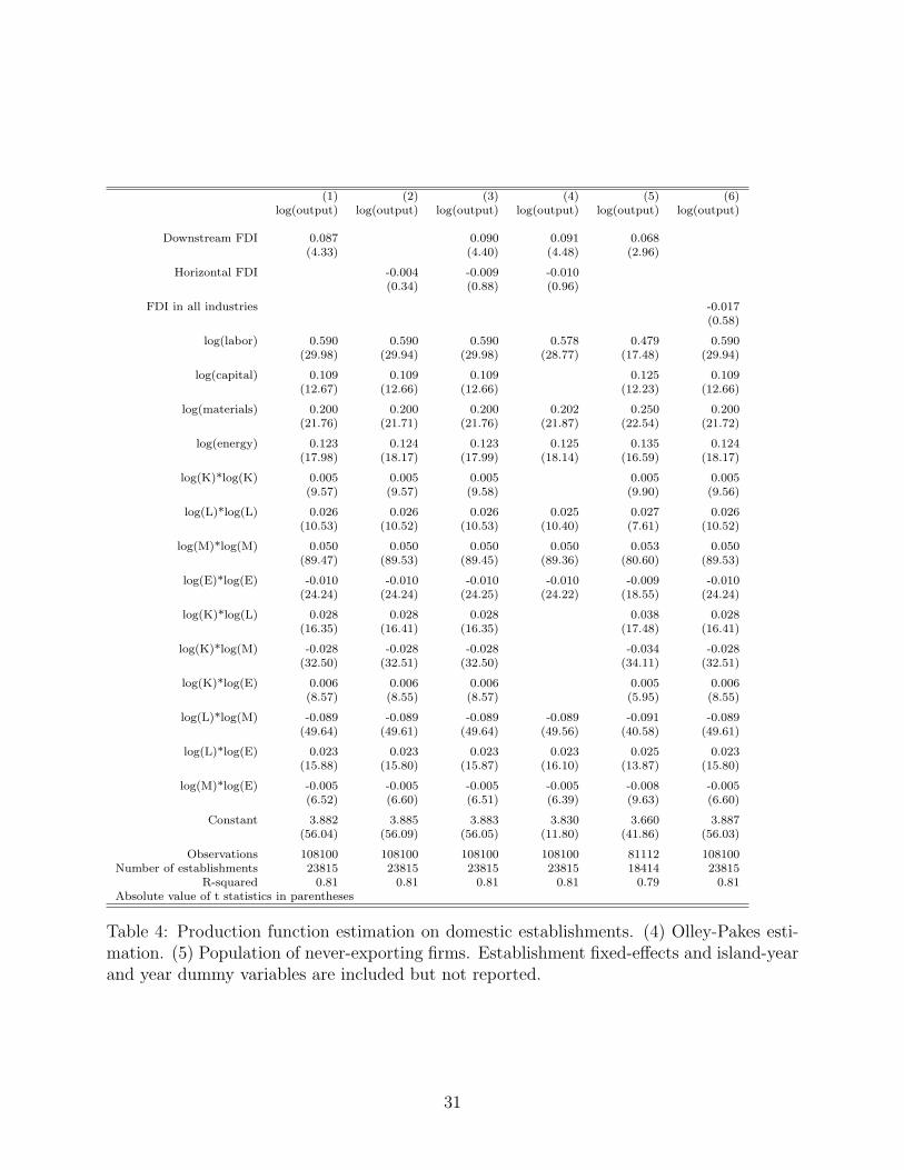
Table 4 reports the results of estimating Equation 1 using an establishment-level fixed-effect

estimator on a sample of domestic firms.7 Column (1) shows downstream FDI, column (2)

shows horizontal FDI, and column (3) shows the effect of both. The coefficient on horizontal

FDI is close to zero, suggesting that there is little learning from direct foreign competitors.

In contrast, the effect of downstream FDI is large and significant, indicating that firms with

growing FDI downstream acquire technology through the supply chain.

Because the estimation is a log-linear production function, the coefficients approximate

elasticities and have intuitive interpretations. The 0.087 coefficient on downstream FDI

7A Hausman test showed significant correlation between individual establishment effects and the otherregressors, thereby rejecting a random-effects model.

15

suggests that firm output increases over eight percent as the share of foreign ownership

downstream rises from zero to one. In practice, increases in share of downstream FDI of

approximately 20 percent are not unusual, suggesting that the actual realized productivity

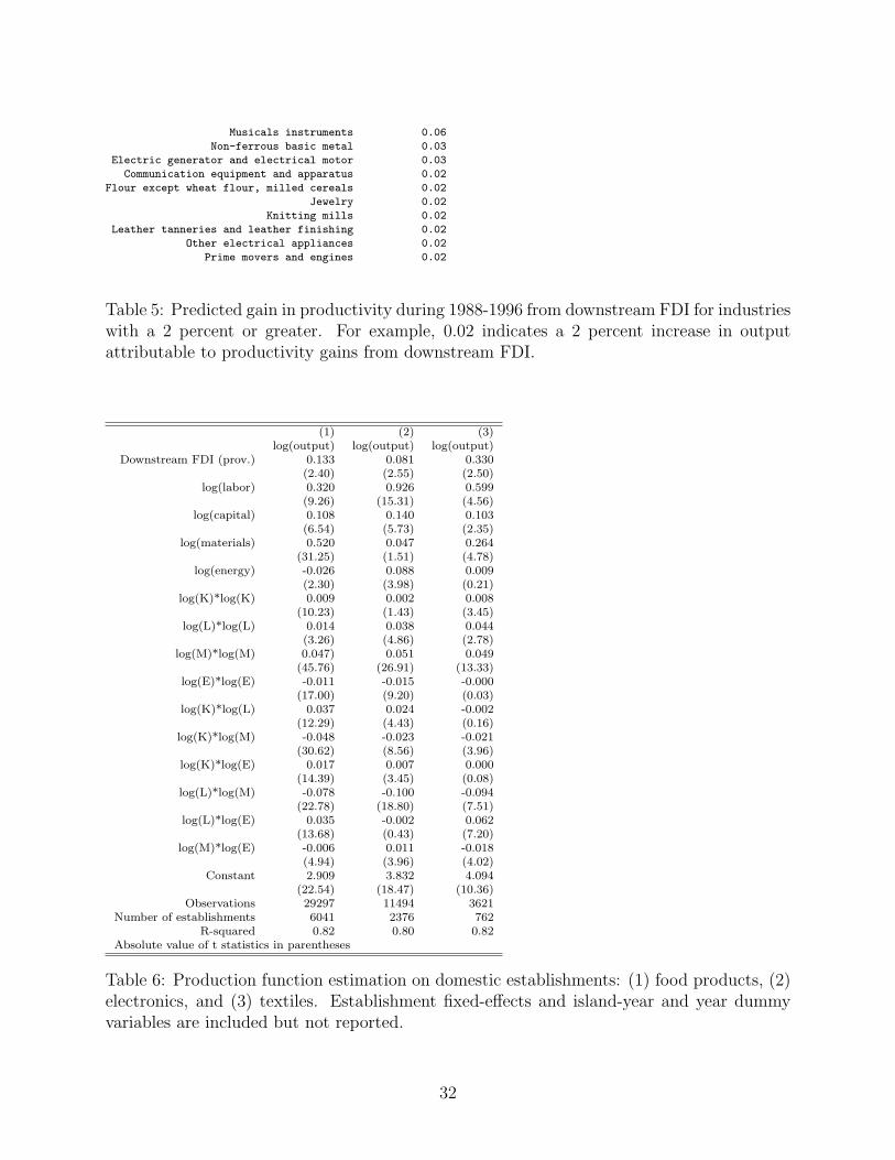
gain might be close to 2 percent (0.2 times 0.087). Table 5 shows the estimated productivity

gain based on the 0.087 point estimate and the actual change in downstream FDI for the

industries with a predicted gain of 2 percent or greater during 1988-1996.

We next perform several checks to examine the robustness of these results.

5.2.1 Potential Simultaneity Bias

The positive correlation between downstream FDI and domestic factory productivity could

result from multinationals selectively locating in areas where supplier productivity was im-

proving. That is, productivity shocks could simultaneously determine downstream FDI and

measured performance. Fixed-effect estimation allows some establishments to be inherently

more productive than others, but assumes that the conditions that make some factories “bet-

ter” remain unchanged. Suppose, however, that establishments were affected by productivity

shocks during the interim of the panel. Such a shock, e.g., the hiring of a skilled manager or

the discovery of a better production technique, is potentially observable to both the supplier

and potential investors, but would remain unobservable to the econometrician. If either local

factories or multinationals reacted to those shocks by adjusting inputs or investment, then

the error term in Equation 1 would not be independent of other right-hand-side variables.

Of particular concern, such simultaneity would introduce correlation between the error term

εit and Downstream FDIjrt.

The error term in Equation 1 can be decomposed to show potential sources of productivity

shocks:

εit = εi + εjt + εrt + εit

One can consider the error term for factory i at time t to consist of four (and potentially

more) sources of error: εi, a static “fixed-effect” for factory i, εjt, a shock to industry j at

16

time t, εrt, a shock to region r at time t, and a fully idiosyncratic shock, εit, affecting factory i

at time t. The fixed-effect estimator controls for the error term εi by only admitting variation

about a factory’s mean. We control for region shocks, such as political strife or government

intervention, by including dummy variables for the interaction of year and island. We will

control for industry-level shocks with by-industry estimations below.

Other variation in the error terms, such as a factory-specific shock or a shock to a par-

ticular industry in a particular region, is captured in the idiosyncratic error term, εit. In

practice, it seems unlikely that εit would be correlated with Downstream FDI; the long lead

time and high transaction costs of investment and contracting with suppliers suggest that

multinationals would invest in industries and regions which offered long-term productivity

growth potential rather than chasing transient boosts to supplier performance. Further, if

supply markets are competitive, shocks affecting just one supplier may have little effect on

market prices. Nonetheless, the possibility of bias remains. Moreover, unobserved produc-

tivity shocks could be correlated with other inputs, such as capital, although the direction

of such a simultaneity bias on the Downstream FDI coefficient is not clear.

Olley and Pakes 1996 proposes using investment as a proxy for idiosyncratic shocks.

The identifying assumption in Olley-Pakes estimation is that investment is monotonically

increasing with respect to the shock, conditional on capital. Because capital responds to the

shock only in a lagged fashion through contemporaneous investment, the return to the other

inputs can be obtained by non-parametrically inverting investment and capital to proxy

for the unobserved shock. Appendix E summarizes the Olley-Pakes estimation approach.

Although it is possible to obtain the return to capital variables with an optional second stage

of estimation, we do not implement that here since capital is not a variable of interest.8

Column (4) of Table 4 shows the results of the Olley-Pakes estimation. The effect of

downstream FDI is statistically identical to that measured without the Olley-Pakes correc-

8An additional concern expressed in Olley and Pakes 1996 is that of survivorship bias. If downstream FDIwas associated with differences in factory survival probability, then changes in the composition of survivingfactories could be confounded with changes in individual factories. In our sample, logit estimates of firmdeaths reveal no significant correlation between downstream FDI and survival probabilities.

17

tion, suggesting that simultaneity bias is not driving the contribution of downstream FDI to

upstream supplier productivity.

Consistent with the arguments in Rodrik (1999) and findings in Aitken and Harrison

(1999) and Javorcik (2004), none of our models provide any evidence of horizontal technology

transfer. The remainder of our analysis focuses on the salient effects of downstream FDI.

5.2.2 Correlation with Exporting Activity

The results so far reveal only the effect on local firms supplying multinationals that operate

within Indonesia. Many of the mechanisms for technology transfer, however, would also

benefit local firms that exported. Indeed, one would expect some correlation between local

firms that supply multinationals within the country and local firms that export. To the

extent that local exporters produce products of international quality and price, in-country

multinationals would be likely to select them as suppliers. Further, to the extent that

local suppliers learn from multinational customers and improve quality and price, they are

more able to export successfully to global markets. Indeed, the factory interviews suggested

that multinational customers may sometimes assist their local suppliers in accessing export

markets.9

To remove any effects of exporting, we estimated Equation 1 on a sample including only

never-exporting domestic firms. Column (5) of Table 4 shows that the positive effect of

downstream FDI holds and suggests that exports are not a viable alternative explanation

for the observed productivity gains.

5.2.3 Public Goods from FDI

The correlation between downstream FDI and local plant productivity could be explained by

multinationals’ provision of public goods rather than by technology transfer. For example,

9See Clerides, Lach, and Tybout 1998, Bernard and Jensen 1999, Aw, Chung, and Roberts 2000, Delgado,Farinas, and Ruano 2002 Van Biesebroeck 2003 and Blalock and Gertler 2004 for discussion of firm learningand exporting.

18

if multinational entry leads to the building of new roads or the installation of more reliable

electricity-generating facilities, then local firm productivity may increase without any transfer

of technology. Since the provision of these public goods would likely be correlated with

downstream FDI, analysis could erroneously attribute local firm gains from public goods to

technology transfer.

To test for the role of public goods, we assume that all plants would benefit from the pro-

vision of roads, bridges, ports, etc. Although some industries would benefit more than others,

this proposition seems reasonable on the grounds that public goods are non-excludable. We

then estimate Equation 1 substituting Region FDIrt, the share of foreign firm share of in-

dustrial output in all industries, for Downstream FDIjrt. Column (6) of Table 4 shows the

insignificant coefficient on Region FDI, indicating that public goods do not have a major

impact on local firm productivity.

5.2.4 By-industry Analysis

The analysis above pools factories in all industries. The advantage of a pooled cross-industry

sample is that it provides high variation in downstream FDI. Recall that downstream FDI is

calculated by industry, region, and year. Because the estimation uses fixed-effect estimation,

only the variation about a factory’s mean, or within variation, is admitted. If the estimation

sample were limited to firms in just one industry, the only between-plant variation in down-

stream FDI would be by region. That is, one would take factories in regions with changes

in downstream FDI over time as the treatment group, and those in other regions with no

changes in downstream FDI as the control group. In practice, we use Indonesia’s 27 provinces

as regional indicators and many industries are concentrated in only a few provinces. Thus,

there is insufficient variation between provinces for a statistically powerful test. Further, if

there is little change in downstream FDI in the industry, there may be insufficient within-

plant variation. To increase variation, we have pooled all industries together. The estimation

then takes some industries as treatment groups and other industries as control groups.

19

A pooled sample, however, has two disadvantages. First, because the effect of downstream

FDI is also constrained to be uniform across industries, one cannot see which industries

benefit from downstream FDI. Second, a pooled sample constrains the return to inputs to

be constant across industries. It may be unreasonable to assume that the marginal product

of capital or labor is uniform across industries as varied as fish processing and electronics

assembly. Such a constraint could bias the results, although it is not obvious in what

direction.

To balance the need for variation in downstream FDI and the desire to have industries

with similar technologies in the treatment and control groups, we selected three groups: a

food group, a textile group, and an electronics group. These groups correspond to the 31,

32, and 38 2-digit ISIC codes respectively, which span several IO codes each and have large

between- and within-establishment downstream FDI. Table 6 shows the results of estimating

Equation 1 on the three samples. The results indicate a strong benefit from downstream

FDI in all three sectors.

5.2.5 Price Heterogeneity

Our framework suggests that multinationals transfer technology to suppliers to reduce in-

put prices and increase quality. The coupling of technology transfer with price reductions

introduces a complication in productivity estimation. Recall that we measure firm output

as nominal revenue deflated by the industry price index. In a competitive market with ho-

mogenous goods, our measure will perfectly correlate with the number of units produced.

In differentiated markets, however, technology transfer might selectively affect the prices of

the recipient firms and, by extension, their estimated unit output.10

Fortunately, the likely direction of productivity bias from price heterogeneity is opposite

to our findings. Suppose the probable case that foreign buyers obtain lower prices from

their suppliers and that these price reductions are not reflected in the industry price index.

10See Melitz 2000 and Katayama, Lu, and Tybout 2003 for a detailed discussion of the estimation concerns.

20

Deflation would thus understate the unit output of technology-recipient firms and downward

bias the measured effect of downstream FDI for the industry overall.

An alternative argument is to consider an industry with little product differentiation. A

market of largely commodity inputs and outputs is less likely to demonstrate price hetero-

geneity across firms. The strong effect of downstream FDI in the textile industry, often an

example of a non-differentiated industry, suggests that it is technology transfer that explains

the productivity gains of domestic supply industries.

6 Market and Welfare Effects

The previous section, we believe, provides evidence that productivity increases when the

share of output purchased by foreign firms rises. This is consistent with downstream foreign-

owned firms transferring technology to upstream suppliers. In this section, we examine the

market and welfare consequences of transferring this technology and test whether it results

in Pareto improvements in welfare as hypothesized in Pack and Saggi 2001. In particular, we

test the hypotheses that technology transfer upstream to suppliers resulted in entry, lower

prices, increased output, and higher profitability in the upstream market; and that the lower

supply prices lead to entry, lower prices, increased output, and increased profitability in the

downstream market.

6.1 Methods and Identification

Again, we are not able to directly measure the transfer of technology. Rather, we measure

the sectors and location where and when foreign companies entered downstream of local

companies. We examine the effect of changes in the share of output purchased by foreign

firms on prices, concentration, and profitability in the supply sector. Specifically, we estimate

21

several reduced form models. Equation 4 measures the effect of FDI on concentration.

HIsrt = β0Downstream FDIjrt + αsr + λgt + γt + εsrt (4)

where HIsrt is the Herfindahl concentration index for 5-digit ISIC sector s in region r in

time t. Note that we use the 89 IO table codes, indicated by subscript j, to define sectors for

supply chains. However, for calculating concentration indexes, which do not require the IO

table, one can more narrowly define industries by the 329 ISIC codes, indicated by subscript

s. αsr is a fixed-effect for the interaction of sector s and region r, λgt is intended to capture

time-variant conditions affecting particular island groupings of the country, and εsrt is an

error term.

Equation 5 measures the effect of FDI on prices.

Pricest = β0Downstream FDIjt + αs + γt + εst (5)

Because prices are not available at the regional level, we use Downstream FDI at the

national level here. That is, downstream FDI is calculated as if the entire country were one

region.

Equations 6 and 7 measure the effect of FDI on firm output and value added respectively.

We define value added as revenue minus wages and the cost of materials and energy. This

is similar to EBITDA (earnings before interest, taxes, depreciation, and amortization), a

common proxy for profitability.

Yit = β0Downstream FDIjrt + αi + λgt + γt + εit (6)

V Ait = β0Downstream FDIjrt + αi + λgt + γt + εit (7)

We then consider the hypotheses regarding feedback to downstream markets, in particu-

lar, that the lower supply prices induce entry, lower prices, and higher profits. We test this

22

hypothesis by examining the effects of changes in foreign ownership in sectors purchasing

from the focal supply sector on the performance of other sectors supplied by that focal sector.

In other words, we ask what is the effect of buying from sectors that supply multinationals

and call this measure suppliers’ downstream FDI. We measure suppliers’ downstream FDI

as the value of downstream FDI in each of the sectors upstream of the focal sector weighted

by the share of focal sector inputs provided by that sector.

Suppliers′ Downstream FDIjrt =∑

k

αjktDownstream FDIkrt (8)

where αjkt is the share of sector j inputs obtained from sector k.

We then re-estimate equations 4-7 replacing downstream FDI with suppliers’ downstream

FDI to gauge the welfare effects in sectors downstream of those sectors supplying multina-

tionals.

6.2 Market and Welfare Results

We estimate the effect of FDI on concentration and prices at the market level—province

markets in the case of concentration and national markets in the case of prices, for which we

do not have regional variation. The effect of FDI on output and value added is calculated

at the firm level.

6.2.1 Concentration and Price

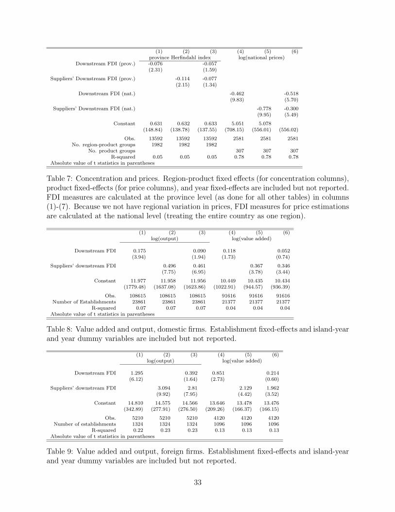
Table 7 contains the estimations of equations 4 and 5. Columns (1)-(3) show estimates of

regional market concentration with a fixed effect for each 5-digit ISIC product and province

cell. Both downstream FDI and suppliers’ downstream FDI are significantly associated

with a decrease in market concentration, measured by a Herfindahl index. This association

suggests that foreign entry downstream will lead to more competition in upstream supply

markets. Likewise, other sectors downstream of those upstream markets also show increases

23

in competition.

Columns (4)-(6) display the effect of FDI on prices estimated by Equation 5. Because we

do not have regional variation in prices, the identifying estimation is by industry and year.

Although one may be cautious in assigning causality from such a reduced form estimation,

the results are consistent with the notion that FDI competition lowers prices. In fact,

downstream FDI and supplier’s downstream FDI are both associated with a decline in prices.

6.2.2 Output and Value Added

We next estimate establishment output and value added. Given that FDI lowers prices, one

expects to see an increase in output. Indeed, columns (1)-(5) of Table 8 show the effect of

FDI on domestic firm output by estimating Equation 6. Both downstream FDI and suppliers’

downstream FDI increase output, likely through the effect of FDI on prices and the demand

added by the new entry. Columns (4)-(6) estimate Equation 7 to show whether domestic

firms capture any of the surplus generated from lower prices and higher output. Again, both

downstream FDI and suppliers’ downstream FDI lead to greater value added, suggesting

that firms are capturing some of the welfare benefits of vertical technology transfer.

Table 9 estimates Equations 6 and 7 on the population of just foreign firms. As was the

case with domestic firms, an increase in downstream FDI and suppliers’ downstream FDI is

associated with increases in both volume and value added.

6.3 Magnitude of Welfare Effects

Since technology transfer from FDI appears to lower prices and increase output and valued

added, there should be a Pareto improvement in welfare. To gauge the magnitude of the

welfare effect, we calculate a simple “back of the envelope” estimation of producer and

consumer surplus gains resulting from FDI in Indonesia during the period of our panel. Our

estimates of the effect are lower bound estimates as they only include the manufacturing

sectors.

24

To gauge producer surplus, we use the estimation results of Equation 7 to calculate the

effect of FDI on value added, which we take as a proxy for profit. To gauge consumer surplus,

we assume a linear demand curve and a supply curve shifting outward from productivity

gains. The increase consumer surplus from 1988 to 1996 is then easily calculated as (p1988 −

p1996) ∗ q1988 + .5(q1996 − q1988) ∗ (p1996 − p1988).

Initial prices, quantity, and value added in 1988 are given in the data. We forecasted

1996 values by adding the product of the coefficients of downstream FDI and suppliers’

downstream FDI and the actual change in FDI by industry. For example, p1996 = p1988 +

β0 ∗ ∆Downstream FDI + β1 ∗ ∆Suppliers′ Downstream FDI, where β0 and β1 are the

coefficients estimated above.

We first estimate the increase in annual producer surplus from 1988 to 1996. Our simple

calculation shows that producer surplus increased by 1.1 percent in intermediate goods sec-

tors, defined as industries that sell 50 percent or more of their output to other manufacturing

sectors, and by 0.7 percent in final goods sectors. Looking at consumer surplus, we find an

increase 5.8 percent relative to total sales in final goods sectors. Although it appears that

consumers are the larger beneficiaries of welfare gains from FDI, we must remember that

the differing approximations for the two surplus could account for part of the magnitude

gap. Although only rough approximations, the producer and consumer surplus measures are

substantial and support our assertion that the effect of FDI is Pareto improving.

7 Summary and Implications

Our findings have two key implications. First, FDI is a source of technology in emerging

markets. Second, this technology generates welfare benefits that may warrant pubic policy

intervention.

The econometric analysis suggests that vertical supply chains are a conduit for technology

transfer from FDI. Indonesian factories in industries in regions with growing downstream FDI

25

experience greater productivity growth, ceteris paribus, than other factories. This finding is

consistent with the incentives of multinational enterprises, which only realize the full benefit

of investment abroad if they can procure high-quality inputs at low cost. To build efficient

supply chains overseas, many multinationals will strategically transfer technology to local

vendors.

The observation of technology transfer alone is insufficient to inform public policy. If

the full benefit of FDI is internalized between the two private parties, then there is no

need for government intervention. Our results show that FDI does indeed generate an

externality—lower prices and greater output—that benefits suppliers, final goods makers,

and consumers. Because the benefits of FDI to the economy exceed the private returns to

both the multinational and its direct suppliers, the total amount of FDI may be less than

the socially optimal amount without intervention.

On the basis of the outcomes we have observed, we conclude that host economy policy-

makers should, at a minimum, not raise barriers to FDI. In cases where there is potential

for multinationals to source supplies from local suppliers, policymakers should consider pro-

viding incentives to encourage FDI.

26

References

Aitken, Brian J., and Ann E. Harrison (1999): “Do Domestic Firms Benefit fromDirect Foreign Investment? Evidence from Venezuela,” American Economic Review, 89(3),605–618.

Aw, Bee Yan, Sukkyun Chung, and Mark J. Roberts (2000): “Productivity andTurnover in the Export Market: Micro-level Evidence from the Republic of Korea andTaiwan (China),” The World Bank Economic Review, 14(1), 65–90.

Bernard, Andrew B., and J. Bradford Jensen (1999): “Exceptional Exporter Per-formance: Cause, Effect, or Both?,” Journal of International Economics, 47(1), 1–25.

Blalock, Garrick (2002): “Technology Adoption from Foreign Direct Investment andExporting: Evidence from Indonesian Manufacturing,” Ph.D. thesis, University of Cali-fornia, Berkeley, Haas School of Business.

Blalock, Garrick, and Paul J. Gertler (2004): “Learning from Exporting Revisitedin a Less Developed Setting,” Journal of Development Economics, 2(75), 397–416.

Blomstrom, Magnus, and Edward N. Wolff (1994): “Multinational Corporationsand Productivity Convergence in Mexico,” in Convergence of Productivity: Cross-NationalStudies and Historical Evidence, ed. by W. J. Baumol, R. R. Nelson, and E. N. Wolff.Oxford University Press, New York.

Clerides, Sofronis K., Saul Lach, and James R. Tybout (1998): “Is Learning byExporting Important? Micro-Dynamic Evidence from Colombia, Mexico, and Morocco,”Quarterly Journal of Economics, 113(3), 903–947.

Delgado, Miguel A., Jose C. Farinas, and Sonia Ruano (2002): “Firm Productivityand Export Markets: A Non-parametric Approach,” Journal of International Economics,57, 397–422.

Goeltom, Miranda S. (1995): Indonesia’s Financial Liberalization: An Empirical Anal-ysis of 1981-88 Panel Data, Iseas Current Economic Affairs Series. ASEAN EconomicResearch Unit, Institute of Southeast Asian Studies, Singapore.

Haddad, Mona, and Ann Harrison (1993): “Are There Positive Spillovers from DirectForeign Investment? Evidence from Panel Data for Morocco,” Journal of DevelopmentEconomics, 42(1), 51–74.

Haskel, Jonathan E., Sonia C. Pereira, and Matthew J. Slaughter (2002):“Does Inward Foreign Direct Investment Boost the Productivity of Domestic Firms?,”Discussion Paper 8433, National Bureau of Economic Research, Cambridge, MA, August.

Hill, Hal (1988): Foreign Investment and Industrialization in Indonesia, East Asian SocialScience Monographs. Oxford University Press, Singapore and New York.

27

Javorcik, Beata Smarzynska (2004): “Does Foreign Direct Investment Increase theProductivity of Domestic Firms? In Search of Spillovers through Backward Linkages,”American Economic Review, 94(3), 605–627.

Katayama, Haijime, Shihua Lu, and James Tybout (2003): “Why Plant-Level Pro-ductivity Studies are Often Misleading, and an Alternative Approach to Interference,”Working Paper 9617, National Bureau of Economic Research, Cambridge, MA.

Keller, Wolfgang (2004): “International Technology Diffusion,” Journal of EconomicLiterature, 42, 752–782.

Kenney, Martin, and Richard L. Florida (1993): Beyond Mass Production: TheJapanese System and Its Transfer to the U.S. Oxford University Press, New York.

Kokko, Ari (1994): “Technology, Market Characteristics, and Spillovers,” Journal of De-velopment Economics, 43(2), 279–293.

Lall, Sanjaya (1980): “Vertical Inter-Firm Linkages in LDCS: An Empirical Study,”Oxford Bulletin of Economics and Statistics, 42, 203–226.

Macduffie, John Paul, and Susan Helper (1997): “Creating Lean Suppliers: DiffusingLean Production through the Supply Chain,” California Management Review, 39(4), 118–151.

Melitz, Marc (2000): “Estimating Firm-Level Productivity in Differentiated ProductIndustries,” Working paper, Harvard University, Department of Economics.

Moran, Theodore H. (2001): Parental Supervision: The New Paradigm for ForeignDirect Investment and Development. Institute for International Economics, Washington,DC.

Nasution, Anwar (1995): “The Opening-up of the Indonesian Economy,” in IndonesianEconomy in the Changing World, ed. by D. Kuntjoro-Jakti, and K. Omura, vol. 32. Insti-tute of Developing Economies, Tokyo.

Olley, G. Steven, and Ariel Pakes (1996): “The Dynamics of Productivity in theTelecommunications Equipment Industry,” Econometrica, 64(6), 1263–1297.

Pack, Howard, and Kamal Saggi (2001): “Vertical Technology Transfer Via Interna-tional Outsourcing,” Journal of Development Economics, 65(2), 389–415.

Pangestu, Mari (1996): Economic Reform, Deregulation, and Privatization: The Indone-sian Experience. Centre for Strategic and International Studies, Jakarta.

Pangestu, Mari, and Yuri Sato (1997): Waves of Change in Indonesia’s ManufacturingIndustry. Institute of Developing Economies, Tokyo.

Rodrik, Dani (1999): “The New Global Economy and Developing Countries: MakingOpenness Work,” Policy Essay 24, Overseas Development Council; Johns Hopkins Uni-versity Press, Washington, DC.

28

Van Biesebroeck, Johannes (2003): “Exporting Raises Productivity in Sub-SaharanAfrican Manufacturing,” Working Paper 10020, National Bureau of Economic Research,Cambridge, MA, October.

Wie, Thee Kian (1994): “Intra-Regional Investment and Technology Transfer in In-donesia,” in Symposium on Intra-Regional Investment and Technology Transfer, ed. byK. Yanagi, pp. 137–166, Kuala Lumpur. Asian Productivity Organization.

World Bank (1993): “Foreign Direct Investment—Benefits Beyond Insurance,” Develop-ment Brief 14, Development Economics Vice-Presidency, Washington, DC, April.

29

A Tables

Capital, materials, energy, and value added are reported in thousands of 1988 rupiah.

domestic foreign1988 log(capital) 11.257 14.086

employees 124 364log(materials) 11.171 14.421

log(energy) 7.388 8.881log(value added) 10.438 14.068

log(value added per worker) 6.447 8.765

1996 log(capital) 11.691 14.659employees 147 584

log(materials) 11.588 14.893log(energy) 7.347 8.618

log(value added) 11.039 14.580log(value added per worker) 6.973 8.967

Table 1: Descriptive statistics by foreign and domestic firms, 1988 and 1996.

Variable Downstream FDI Horizontal FDI Suppliers’ Downstream FDIDownstream FDI 1.00

Horizontal FDI 0.34 1.00Suppliers’ Downstream FDI 0.55 0.44 1.00

Table 2: Correlation between measures of FDI.

Year No. Domestic Firms No. Foreign Firms Horizontal FDI Downstream FDI Suppliers’ Downstream FDI1988 8888 276 .131 .060 .0741996 14912 888 .232 .094 .118

Table 3: Foreign and domestic establishment count, mean horizontal, downstream, andsuppliers’ downstream FDI, 1988 and 1996.

30

(1) (2) (3) (4) (5) (6)log(output) log(output) log(output) log(output) log(output) log(output)

Downstream FDI 0.087 0.090 0.091 0.068(4.33) (4.40) (4.48) (2.96)

Horizontal FDI -0.004 -0.009 -0.010(0.34) (0.88) (0.96)

FDI in all industries -0.017(0.58)

log(labor) 0.590 0.590 0.590 0.578 0.479 0.590(29.98) (29.94) (29.98) (28.77) (17.48) (29.94)

log(capital) 0.109 0.109 0.109 0.125 0.109(12.67) (12.66) (12.66) (12.23) (12.66)

log(materials) 0.200 0.200 0.200 0.202 0.250 0.200(21.76) (21.71) (21.76) (21.87) (22.54) (21.72)

log(energy) 0.123 0.124 0.123 0.125 0.135 0.124(17.98) (18.17) (17.99) (18.14) (16.59) (18.17)

log(K)*log(K) 0.005 0.005 0.005 0.005 0.005(9.57) (9.57) (9.58) (9.90) (9.56)

log(L)*log(L) 0.026 0.026 0.026 0.025 0.027 0.026(10.53) (10.52) (10.53) (10.40) (7.61) (10.52)

log(M)*log(M) 0.050 0.050 0.050 0.050 0.053 0.050(89.47) (89.53) (89.45) (89.36) (80.60) (89.53)

log(E)*log(E) -0.010 -0.010 -0.010 -0.010 -0.009 -0.010(24.24) (24.24) (24.25) (24.22) (18.55) (24.24)

log(K)*log(L) 0.028 0.028 0.028 0.038 0.028(16.35) (16.41) (16.35) (17.48) (16.41)

log(K)*log(M) -0.028 -0.028 -0.028 -0.034 -0.028(32.50) (32.51) (32.50) (34.11) (32.51)

log(K)*log(E) 0.006 0.006 0.006 0.005 0.006(8.57) (8.55) (8.57) (5.95) (8.55)

log(L)*log(M) -0.089 -0.089 -0.089 -0.089 -0.091 -0.089(49.64) (49.61) (49.64) (49.56) (40.58) (49.61)

log(L)*log(E) 0.023 0.023 0.023 0.023 0.025 0.023(15.88) (15.80) (15.87) (16.10) (13.87) (15.80)

log(M)*log(E) -0.005 -0.005 -0.005 -0.005 -0.008 -0.005(6.52) (6.60) (6.51) (6.39) (9.63) (6.60)

Constant 3.882 3.885 3.883 3.830 3.660 3.887(56.04) (56.09) (56.05) (11.80) (41.86) (56.03)

Observations 108100 108100 108100 108100 81112 108100Number of establishments 23815 23815 23815 23815 18414 23815

R-squared 0.81 0.81 0.81 0.81 0.79 0.81Absolute value of t statistics in parentheses

Table 4: Production function estimation on domestic establishments. (4) Olley-Pakes esti-mation. (5) Population of never-exporting firms. Establishment fixed-effects and island-yearand year dummy variables are included but not reported.

31

Musicals instruments 0.06

Non-ferrous basic metal 0.03

Electric generator and electrical motor 0.03

Communication equipment and apparatus 0.02

Flour except wheat flour, milled cereals 0.02

Jewelry 0.02

Knitting mills 0.02

Leather tanneries and leather finishing 0.02

Other electrical appliances 0.02

Prime movers and engines 0.02

Table 5: Predicted gain in productivity during 1988-1996 from downstream FDI for industrieswith a 2 percent or greater. For example, 0.02 indicates a 2 percent increase in outputattributable to productivity gains from downstream FDI.

(1) (2) (3)log(output) log(output) log(output)

Downstream FDI (prov.) 0.133 0.081 0.330(2.40) (2.55) (2.50)

log(labor) 0.320 0.926 0.599(9.26) (15.31) (4.56)

log(capital) 0.108 0.140 0.103(6.54) (5.73) (2.35)

log(materials) 0.520 0.047 0.264(31.25) (1.51) (4.78)

log(energy) -0.026 0.088 0.009(2.30) (3.98) (0.21)

log(K)*log(K) 0.009 0.002 0.008(10.23) (1.43) (3.45)

log(L)*log(L) 0.014 0.038 0.044(3.26) (4.86) (2.78)

log(M)*log(M) 0.047) 0.051 0.049(45.76) (26.91) (13.33)

log(E)*log(E) -0.011 -0.015 -0.000(17.00) (9.20) (0.03)

log(K)*log(L) 0.037 0.024 -0.002(12.29) (4.43) (0.16)

log(K)*log(M) -0.048 -0.023 -0.021(30.62) (8.56) (3.96)

log(K)*log(E) 0.017 0.007 0.000(14.39) (3.45) (0.08)

log(L)*log(M) -0.078 -0.100 -0.094(22.78) (18.80) (7.51)

log(L)*log(E) 0.035 -0.002 0.062(13.68) (0.43) (7.20)

log(M)*log(E) -0.006 0.011 -0.018(4.94) (3.96) (4.02)

Constant 2.909 3.832 4.094(22.54) (18.47) (10.36)

Observations 29297 11494 3621Number of establishments 6041 2376 762

R-squared 0.82 0.80 0.82Absolute value of t statistics in parentheses

Table 6: Production function estimation on domestic establishments: (1) food products, (2)electronics, and (3) textiles. Establishment fixed-effects and island-year and year dummyvariables are included but not reported.

32

(1) (2) (3) (4) (5) (6)province Herfindahl index log(national prices)

Downstream FDI (prov.) -0.076 -0.057(2.31) (1.59)

Suppliers’ Downstream FDI (prov.) -0.114 -0.077(2.15) (1.34)

Downstream FDI (nat.) -0.462 -0.518(9.83) (5.70)

Suppliers’ Downstream FDI (nat.) -0.778 -0.300(9.95) (5.49)

Constant 0.631 0.632 0.633 5.051 5.078(148.84) (138.78) (137.55) (708.15) (556.01) (556.02)

Obs. 13592 13592 13592 2581 2581 2581No. region-product groups 1982 1982 1982

No. product groups 307 307 307R-squared 0.05 0.05 0.05 0.78 0.78 0.78

Absolute value of t statistics in parentheses

Table 7: Concentration and prices. Region-product fixed effects (for concentration columns),product fixed-effects (for price columns), and year fixed-effects are included but not reported.FDI measures are calculated at the province level (as done for all other tables) in columns(1)-(7). Because we not have regional variation in prices, FDI measures for price estimationsare calculated at the national level (treating the entire country as one region).

(1) (2) (3) (4) (5) (6)log(output) log(value added)

Downstream FDI 0.175 0.090 0.118 0.052(3.94) (1.94) (1.73) (0.74)

Suppliers’ downstream FDI 0.496 0.461 0.367 0.346(7.75) (6.95) (3.78) (3.44)

Constant 11.977 11.958 11.956 10.449 10.435 10.434(1779.48) (1637.08) (1623.86) (1022.91) (944.57) (936.39)

Obs. 108615 108615 108615 91616 91616 91616Number of Establishments 23861 23861 23861 21377 21377 21377

R-squared 0.07 0.07 0.07 0.04 0.04 0.04Absolute value of t statistics in parentheses

Table 8: Value added and output, domestic firms. Establishment fixed-effects and island-yearand year dummy variables are included but not reported.

(1) (2) (3) (4) (5) (6)log(output) log(value added)

Downstream FDI 1.295 0.392 0.851 0.214(6.12) (1.64) (2.73) (0.60)

Suppliers’ downstream FDI 3.094 2.81 2.129 1.962(9.92) (7.95) (4.42) (3.52)

Constant 14.810 14.575 14.566 13.646 13.478 13.476(342.89) (277.91) (276.50) (209.26) (166.37) (166.15)

Obs. 5210 5210 5210 4120 4120 4120Number of establishments 1324 1324 1324 1096 1096 1096

R-squared 0.22 0.23 0.23 0.13 0.13 0.13Absolute value of t statistics in parentheses

Table 9: Value added and output, foreign firms. Establishment fixed-effects and island-yearand year dummy variables are included but not reported.

33

B Figures

11

Em

piric

al S

trat

egy:

Use

Var

iatio

n in

For

eign

Ow

ners

hip

Acr

oss

Mar

kets

/Tim

e

Fin

al S

ecto

r 1

Sup

ply

Sec

tor

Fin

al S

ecto

r 2

Tec

hnol

ogy

tran

sfer

For

eign

F

irm 2

Loca

l S

uppl

y 2

Loca

l S

uppl

y 1

Loca

l F

irm 2

For

eign

F

irm 1

Loca

l F

irm 1

Incr

ease

d pr

oduc

tivity

Ent

ry &

com

petit

ion

Low

er P

rices

In

crea

sed

outp

ut &

v

alue

add

ed

Low

er fi

nal s

ecto

r pr

ices

Incr

ease

d ou

tput

& v

alue

add

ed

Low

er s

uppl

y pr

ices

Figure 1: Flow of technology and welfare effects from FDI.

34

���

�

�

���������

�

Figure 2: Value added in manufacturing, 1996, by province.

35

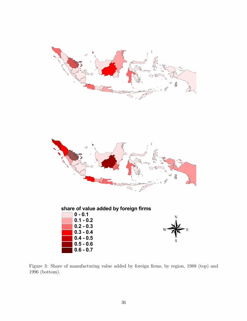
Figure 3: Share of manufacturing value added by foreign firms, by region, 1988 (top) and1996 (bottom).

36

C Data Appendix

C.1 Product Class, Location, and Age

The main product class of each establishment is identified by 5-digit International Standardof Industrial Classification (ISIC) codes published by the United Nations Industrial Devel-opment Organization (UNIDO). The ISIC standard divides manufacturing activity into 329codes at the 5-digit level.11 The data include plant age and location at the province andkabupaten (district) level. The province and district codes divide the country into 27 and304 areas respectively. The analysis in this paper uses province to identify region.12

C.2 Ownership

Two survey questions relate to establishment ownership. First, establishments report whetherthey operate under a domestic or a foreign investment license. All new enterprises in Indone-sia must obtain an operating license from Badan Koordinasi Penanaman Modal (BKPM), theInvestment Coordinating Board. Establishments funded with any foreign investment operateunder Penanaman Modal Asing (PMA), foreign capital investment licenses. Establishmentswith only domestic investment obtain Penanaman Modal Dalam Negeri (PMDN), whollydomestic capital investment licenses. Second, each establishment reports the percentage offoreign equity.13 Establishments with more than 20 percent foreign equity were defined asforeign. This definition yielded a sample of foreign factories very similar to those operatingwith PMA licenses. Estimation with foreign plants defined as those with any foreign equity,or those with more than 50 percent foreign equity, yielded nearly identical results.

C.3 Capital

The survey asks for the book value and current replacement value of fixed assets. Respon-dents report assets in five categories: land, buildings, machinery and equipment, vehicles,and other assets. The value of investment is also reported yearly.

C.4 Labor and Wages

The numbers of production and non-production workers are reported in all years. Cashand in-kind wages are available for production and non-production workers in all years. Inmost years, wage payments are detailed in four categories: normal wages, overtime, gifts andbonuses, and other payments. We used to total of all payments as our measure of wages.

11ISIC codes are revision 1 codes prior to 1990 and revision 2 codes thereafter. The method of concordancebetween the two revisions is discussed in Appendix D.

12Following the independence of East Timor, there are now 26 provinces and 291 districts.13The source country of foreign capital is reported only in the 1988 survey. Although the survey instruments

asked for this information in most years, BPS keypunched the response in only 1988. Sadly, BPS hasdestroyed the original paper survey responses, so this information cannot be retrieved.

37

C.5 Materials and Energy

The value of all consumed materials is reported every year. The data also indicate the quan-tity and cost of consumed petroleum products, e.g., gasoline and lubricants, and purchasedand self-generated electricity.

C.6 Output

The nominal rupiah value of production output is available every year.

D Data Cleaning Appendix

This section provides more detail on the construction and cleaning of the dataset.

D.1 Construction of Price Deflators

Output, materials, and capital are deflated to express values in real terms. The deflatorsare based on Indeks Harga Perdangangan Besar (IHPB), wholesale price indexes (WPI),published monthly in BPS’s Buletin Statistik Bulanan Indikator Ekonomi, the Monthly Sta-tistical Bulletin of Economic Indicators. To calculate WPI, BPS field officers interviewrepresentative firms in all provinces to collect prices for five categories of commodities: agri-culture, manufacturing, mining and quarrying, imports, and exports. In total, prices areavailable for 327 commodities, 192 of which are manufactured commodities.

D.1.1 Output, Materials, and Energy Deflators

Nominal rupiah output and materials values are deflated using the WPI for the nearestcorresponding manufactured commodity. BPS officials provided an unpublished concordancetable mapping the 192 WPI commodity codes to the 329 5-digit ISIC product codes. Energyis deflated using Indonesian petroleum prices.

D.1.2 Capital Deflators

Fixed assets are deflated using the WPI for manufactured construction materials and im-ported machinery. Specifically, the capital deflator combines the WPI for construction mate-rials, imported electrical and non-electrical machinery, and imported transportation equip-ment. We weighted these price indexes by the average reported value shares of buildingand land, machinery, and vehicle fixed assets in the SI survey to obtain an annual capitaldeflator.

D.2 Correction for Outliers and Missing Values in Industrial Sur-veys

We have cleaned key variables to minimize noise due to non-reporting, misreporting, andobvious mistakes in data keypunching. A three-stage cleaning process was used for capital,

38

labor, materials, and energy. First, the earliest and latest years in which a plant reportedwere identified, and interpolation was used to fill-in up gaps of up to two missing years withinthe reporting window. If more than two continous years of data were missing, the factorywas dropped from the sample. The first stage of cleaning removed about 15 percent of thetotal sample. Second, sudden spikes in key data values likely attributable to keypunch error(often due to an erroneously added or omitted zero) were corrected with interpolation. Third,plants with remaining unreasonably large jumps or drops in key variables not accompaniedby corresponding movements in other variables (for example, large increases in labor notaccompanied by any increase in output) were dropped. This third stage removed about 10percent of the sample.

The replacement value of fixed assets is used as the measure of capital stock for mostfactories. For the few factories that reported only the book value of fixed assets, those figureswere used instead.

The percentage of foreign equity in the establishment was cleaned to remove erroneouslyadded or omitted zeros resulting from keypunch error. For example, a factory with foreignequity reported over time as 100, 100, 10, and 100 percent was cleaned to show 100 percentin all years.

D.3 Concordance of Rev. 1 and Rev. 2 ISIC Codes

The industrial survey reports revision 1 ISIC codes prior to 1990 and revision 2 codes there-after. Attempts to create a concordance table at the 5-digit level from rev. 1 to rev. 2 codesyielded disappointing results. Comparing code changes for the same establishment beforeand after 1990 showed that the concordance table predictions were incorrect as often as halfthe time. Rather than accept the noise introduced by these mistakes, the analysis attemptsto assign each establishment’s actual rev. 2 code to its observations in 1988-1989. Specifi-cally, for each establishment that appears in either 1988 or 1989, the analysis looks for theearliest appearance of the same establishment in 1990 and later years. In most cases, therev. 2 code from the 1990 observation could be used. If the establishment did not appearin 1990, the rev. 2 code from 1991 or 1992 was used. If the establishment did not appearbetween 1990 and 1992, it was dropped. This process greatly improved the precision of ISICcode assignments at the cost of dropping about 5 percent of the 1988-1989 sample. Sincethe dropped establishments appear in only one or two years anyway, the 5 percent loss haslittle effect on the results.

D.4 Concordance of Input-Output Table Code and ISIC Codes

The IO table was published in 1990 and 1995 with four variants: domestic transactions atproducer prices, domestic transactions at purchaser prices, domestic and export transactionsat producer prices, and domestic and export transactions at purchaser prices. The analysishere considers domestic transactions at producer prices.

Both the 1990 and 1995 IO tables classified industrial production into 89 categories. Tomerge the IO table with the SI, first the 1995 IO table codes were concorded with the 1990IO table codes. Next, the 1990 IO table codes were concorded with the 329 5-digit ISICcodes reported in the SI. The 1990 IO codes were used to define industries in the analysis.

39

E Olley-Pakes Estimation Appendix

Although a full description of Olley-Pakes estimation is beyond the scope of this paper(interested readers are referred to Olley and Pakes 1996), the steps implemented here arebriefly outlined below.

Because the variable of interest in this study is the return to FDI, which is estimated inthe first of the three estimation stages, we do not implement the second and third stages.However, the latter two stages are briefly described below for reference.

Although we estimated a translog production function, a Cobb-Douglas function is shownbelow for ease of presentation.

The EstimationThe Olley-Pakes estimation consists of three stages. First, investment is used as a proxy

for idiosyncratic shocks to determine the contribution of variable inputs (labor, materials,and energy) conditional on the shock and state variables (capital). Second, the effect of statevariables on factory exit is estimated with a probit model to control for self-selection biasin plant closings. The concern here is that factories with certain state attributes, such aslow levels of capitalization, may be more likely to close if they experience a negative shock.Third, the contribution of state variables is calculated conditional on the prior period’s shockand the likelihood of closure. The assumption driving the identification in this stage is thatstate variables respond to shocks in a lagged manner. That is, the unexpected portion ofthe current period shock does not immediately affect capital or vertical FDI. Rather, onlyinvestment in the current period, which yields capital or vertical FDI in the subsequentperiod, is affected.

STAGE 1The estimation starts with a Cobb-Douglas production function

yit = βexpFDIjrt + βllit + βmmit + βeeit + βkkit (9)

+ ωit + ηit

where ωit is the factory’s idiosyncratic productivity shock (that could affect the factory’schoice of freely variable inputs) and ηit is measurement error (or error that does not affectthe factory’s choice of inputs), and lower case variable names represent logs. Olley and Pakesshow that investment is monotonically increasing in ωit and can hence be used as a proxyfor the shock conditional on state variables. That is, investment, i, can be expressed as afunction of the state variables and the shock.

iit = iit(ωit, kit) (10)

Provided that iit > 0, investment can be inverted to reveal ωit.

ωit = hit(iit, kit) (11)

Conditioning output on ωit and the state variables yields the following semi-parametricestimation.

yit = βexpEXPORTEDjrt + βllit + βmmit + φit(iit, kit) + ηit (12)

40

where

φit(iit, kit) = β0 + βkkit + hit(iit, kit)

Since the error term ηit is uncorrelated with the inputs, estimation of equation 12 providesunbiased estimates of βexp, βl and βm. We use a third-order polynomial expansion in iit andkit to estimate φit.

41