Federal Reserve Bank of Dallas Globalization and Monetary Policy Institute

Working Paper No. 296 https://doi.org/10.24149/gwp296r1

Capital Accumulation and Dynamic Gains from Trade*

B. Ravikumar Ana Maria Santacreu Federal Reserve Bank of St. Louis Federal Reserve Bank of St. Louis

Michael Sposi

Federal Reserve Bank of Dallas January 2017 Revised: March 2018

Abstract We compute welfare gains from trade in a dynamic, multicountry model with capital accumulation and trade imbalances. We develop a gradient-free method to compute the exact transition paths for 44 countries following a trade liberalization. We find that (i) larger countries accumulate a current account surplus and financial resources flow from larger countries to smaller countries boosting consumption in the latter, (ii) countries with larger short-run trade deficits accumulate capital faster, (iii) the gains are nonlinear in the reduction in trade costs, and (iv) capital accumulation accounts for substantial gains. The net foreign asset (NFA) position before the liberalization and the tradeables intensity in investment goods production and consumption goods production are quantitatively important for the gains. JEL codes: E22, F11, O11 Keywords: Welfare gains; Dynamics; Capital accumulation; Trade imbalances

*Ana Maria Santacreu, Federal Reserve Bank of St. Louis, P.O. Box 442, St. Louis, MO 63166. 314-444-6145. am.santacreu@gmail.com. B. Ravikumar, Federal Reserve Bank of St. Louis, P.O. Box 442, St. Louis, MO 63166. 314-444-7312. b.ravikumar@wustl.edu. Michael Sposi, Federal Reserve Bank of Dallas, Research Department, 2200 N. Pearl Street, Dallas, TX 75201. 214-922-5881. michael.sposi@dal.frb.org. This paper benefited from comments by Lorenzo Caliendo, Jonathan Eaton, Cecile Gaubert, Samuel Kortum, Robert E. Lucas Jr., Ellen McGrattan, Marc Melitz, Fernando Parro, Kim Ruhl, Shouyong Shi, Mariano Somale, Nancy Stokey, Felix Tintelnot, Kei-Mu Yi, and Jing Zhang. We are grateful for university seminar audiences at Arizona State, Penn State, Purdue, Texas-Austin, and conference audiences at the Becker-Friedman Institute, EIIT, Midwest Macro, Midwest Trade, North American Summer Econometric Society, RIDGE Trade and Firm Dynamics, UTDT Economics, the Society for Economic Dynamics, Minnesota Macro, Princeton IES, the 2017 NBER ITM SI, and the System Committee for International Economic Analysis. The views in this paper are those of the authors and do not necessarily reflect the views of the Federal Reserve Banks of Dallas and St. Louis or the Federal Reserve System.

1 Introduction

How large are the welfare gains from trade? This is an old and important question. This

question has typically been answered in static settings by computing the change in real

income from an observed equilibrium to a counterfactual equilibrium. In such computations,

the factors of production and technology in each country are held fixed, and the change in

real income is immediate and is entirely due to the change in each country’s trade share

that responds to a change in trade frictions. Recent examples include Arkolakis, Costinot,

and Rodrıguez-Clare (2012) (ACR hereafter), who compute the welfare cost of autarky, and

Waugh and Ravikumar (2016), who compute the welfare gains from frictionless trade.1

By design, the above computations cannot distinguish between static and dynamic gains.

The static gains accrue immediately after a trade liberalization and there is no cost to increas-

ing consumption. Dynamic gains, on the other hand, accrue gradually. For instance, capital

accumulation is costly because it requires foregone consumption. Consumption smoothing

motives imply that capital accumulation is gradual.

We calculate welfare gains from trade in a dynamic multicountry Ricardian model where

international trade affects the capital stock in each country in each period. Our environment

is a version of Eaton and Kortum (2002) embedded in a two-sector neoclassical growth

model, similar to Alvarez and Lucas (2017). There is a continuum of tradable intermediate

goods that are used in the production of investment goods, final consumption goods, and

intermediate goods. Each country is endowed with an initial stock of capital, and investment

goods augment the stock of capital. We add two features that affect the gains: (i) Cross-

country heterogeneity in the tradables intensity in investment goods and in consumption

goods and (ii) endogenous trade imbalances. The first feature affects the cross-country

heterogeneity in the rate of capital accumulation after a trade liberalization and, hence, the

gains from trade. The second feature helps each country smooth its consumption over time

and, hence, affects the gains.

We calibrate the tradables intensity using the World Input Output Database. We cal-

ibrate productivities and trade costs so that the steady state of the model reproduces the

observed bilateral trade flows across 44 countries and the trade imbalances in each country.

We then conduct a counterfactual exercise in which there is an unanticipated, uniform, and

permanent 20 percent reduction in trade frictions in all countries. We compute the exact lev-

els of endogenous variables along the transition path from the calibrated steady state to the

1See Adao, Costinot, and Donaldson (2017) for a nonparametric generalization of ACR.

2

counterfactual steady state and calculate the welfare gains using a consumption-equivalent

measure as in Lucas (1987). Welfare gains from the trade liberalization accrue gradually in

our model and our measure of gains includes the gradual transition from the initial steady

state to the counterfactual steady state.

We find that (i) the current account balance immediately after the liberalization is pos-

itively correlated with size—larger countries accumulate a current account surplus, and fi-

nancial resources flow from larger countries to smaller countries, boosting consumption in

the latter; (ii) half-life for capital accumulation is negatively correlated with short-run trade

deficits—countries with larger short-run trade deficits accumulate capital faster; (iii) gains

from trade are nonlinear—elasticity of gains with respect to reductions in trade costs is

higher for larger reductions; (iv) dynamic gains are 35 percent more than gains in a static

model where capital is fixed; and (v) steady-state gains in a balanced-trade version of our

dynamic model are 80 percent more than the static gains.

Trade liberalization affects the gains in our model through two channels: total factor

productivity (TFP) and capital-labor ratio. The TFP channel is a familiar one in trade

models. Trade liberalization results in a decline in home trade share and, hence, an increase

in TFP, which increases output. This channel affects the level of consumption along the

transition. Trade liberalization also increases the rate of capital accumulation as higher TFP

boosts the returns to capital. As a result, capital accumulates yielding higher output and

consumption along the transition path. The increase in the capital-labor ratio is gradual

as in the neoclassical growth model.2 In addition, trade liberalization increases the rate

of capital accumulation due to the decrease in the relative price of investment. In our

model, investment goods production is more tradables-intensive than consumption goods

production, so trade liberalization lowers the relative price of tradables, which alters the

rate of transformation between consumption and investment, and helps allocate a larger

share of output to investment. This increases the investment rate, thereby further boosting

output and consumption along the transition path. In a static model, the capital-labor ratio

channel is clearly absent.

The role of trade imbalances in generating the gains depends on net foreign asset (NFA)

positions before the liberalization and on the nature of the liberalization. Starting from

an NFA position of zero and balanced trade, gains from an unanticipated liberalization are

not quantitatively affected by asset trades across countries. That is, after the liberalization,

2In a two-country model, Connolly and Yi (2015) examine South Korea’s growth miracle and argue thatreductions in trade costs had quantitatively important effects on steady-state capital stock and income.

3

allowing for endogenous trade imbalances or restricting allocations to balanced trade does

not affect the gains quantitatively. However, if the liberalization is anticipated, then allowing

for endogenous trade imbalances implies more gains relative to a world where each country’s

trade is balanced every period. In a world with asset trades across countries, the initial cross-

country heterogeneity in NFA positions also has important quantitative implications for gains

from liberalization. An unanticipated trade liberalization increases the world interest rate on

impact, which implies that countries with initial debt suffer and countries with initial positive

assets benefit. That is, countries that start with a negative NFA position lose relative to

being in an environment where each country’s initial NFA position is zero.

In our model, there is a propagation from trade imbalances to capital accumulation:

Countries with a trade deficit accumulate capital faster after a trade liberalization and

changes in current rates of capital accumulation affect future trade imbalances which, in

turn, affect future rates of capital accumulation. The propagation is absent in Reyes-Heroles

(2016) who studies global trade imbalances in a model without capital. Furthermore, in

his model, one must choose an ad-hoc terminal NFA position in order to solve for the

counterfactual implications. This is not true in our model since diminishing returns to capital

accumulation and equalization of marginal products of capital (MPKs) across countries imply

a unique counterfactual steady state. As each country’s capital stock adjusts gradually,

current accounts respond in order to equalize the MPKs and the steady-state NFA position

depends on the current account dynamics. Hence, the counterfactual steady state cannot be

determined independently from the initial steady state and the transition.

The tradables intensity in each sector plays an important role in our model. The tradables

intensity in investment goods production determines the transition path for capital after

a trade liberalization and has little effect on TFP dynamics. The tradables intensity in

consumption goods affects the transition path of TFP and has little effect on the dynamics of

capital. Cross-country heterogeneity in the consumption goods tradables intensity accounts

for 26 percent of the log-variance in the gains from trade, whereas cross-country heterogeneity

in the investment goods tradables intensity accounts for only 3 percent.

Investment goods production is typically more tradables-intensive than consumption

goods production, and countries with a larger difference between the two intensities ex-

perience a larger decline in the relative price of investment and a larger increase in the

investment rate. This result is similar to the findings in Mutreja, Ravikumar, and Sposi

(2018), who examine the role of this channel on economic development in a model where

there is no cross-country heterogeneity in the intensities.

4

We provide a fast computational method for solving multicountry trade models with large

state spaces. The state variables in our model include capital stocks as well as NFA positions.

Our algorithm iterates on a subset of prices using excess demand equations and delivers the

entire transition path for 44 countries in less than two hours on a standard computer (see

also Alvarez and Lucas, 2007). Our algorithm uses gradient-free updating rules that are

computationally faster than the nonlinear solvers used in recent dynamic models of trade

(e.g., Eaton, Kortum, Neiman, and Romalis, 2016; Kehoe, Ruhl, and Steinberg, 2016).

Our paper is related to three papers on multicountry models with capital accumulation:

Alvarez and Lucas (2017), Eaton, Kortum, Neiman, and Romalis (2016), and Anderson,

Larch, and Yotov (2015).3 Alvarez and Lucas (2017) approximate the dynamics in a model

with period-by-period balanced trade by linearizing around the counterfactual steady state.

Our computational method provides an exact dynamic path. The linear approximation might

be inaccurate for computing transitional dynamics in cases of large trade liberalizations. For

instance, we find that even with balanced trade the dynamic gain increases exponentially with

reductions in trade frictions. Furthermore, as noted earlier, endogenous trade imbalances

and capital accumulation imply that the counterfactual steady state and the transitional

dynamics have to be solved simultaneously.

Eaton, Kortum, Neiman, and Romalis (2016) examine the collapse of trade during the

recent recession. They quantify the roles of different shocks via counterfactuals by solving

the planner’s problem. In their computation, the Pareto weight for each country is its

share of consumption in world consumption expenditures and the weight is the same in the

benchmark and in the counterfactual. Instead, we solve for the competitive equilibrium and

find that each country’s consumption share changes in the counterfactual. For example,

Bulgaria’s share increases by 30 percent across steady states, whereas the United States’

share decreases.

Anderson, Larch, and Yotov (2015) compute transitional dynamics in a model where the

relative price of investment and the investment rate do not depend on trade frictions. The

investment rate in their model can be computed once and for all as a constant pinned down

by the structural parameters. The transition path can then be computed as a solution to

a sequence of static problems. In our model, current allocations and prices depend on the

entire path of prices and trade frictions. Hence, we have to simultaneously solve a system

3Baldwin (1992) and Alessandria, Choi, and Ruhl (2014) study welfare gains in two-country models withcapital accumulation and balanced trade (see also Brooks and Pujolas, 2016). Different from two-countrymodels, our multicountry analysis with endogenous trade imbalances exploits rich cross-country heterogeneitythat has a quantitatively important role in capital accumulation and gains from trade.

5

of second-order, non-linear difference equations. Empirically, Wacziarg and Welch (2008)

provide evidence showing an increase in investment rate after trade liberalizations for a

sample of 118 countries, which is consistent with our model’s implication.

Our paper is also related to recent studies that use sufficient statistics in static models.

They measure changes in welfare by changes in income, which are completely described by

changes in the home trade share (e.g., ACR). In our model with endogenous trade imbalances,

changes in the home trade share are not sufficient to characterize the changes in welfare,

because changes in home trade share do not reflect changes in income, and consumption is

not proportional to income in the steady state or along the transition.

The rest of the paper proceeds as follows. Section 2 presents the model with trade

imbalances. Section 3 describes the calibration, and Section 4 reports the results from

the counterfactual exercise. Section 5 explores the role of capital accumulation. Section 6

examines the role of trade imbalances and tradables intensity. Section 7 concludes.

2 Model

There are I countries indexed by i = 1, . . . , I, and time is discrete, running from t = 1, . . . ,∞.

There are three sectors: consumption, investment, and intermediates, denoted by c, x, and

m, respectively. Neither consumption goods nor investment goods are tradable. There is

a continuum of intermediate varieties that are tradable. Trade in intermediate varieties is

subject to iceberg costs. (In Appendix G, we enrich our model with more sectors and a

complete input-output [IO] structure. Every sector’s output is used for intermediate goods

and final goods production, and the final product is used for consumption and investment.)

Each country has a representative household that owns the country’s primary factors of

production, capital, and labor. Capital and labor are mobile across sectors within a country

but are immobile across countries. The household inelastically supplies capital and labor to

domestic firms and purchases consumption and investment goods from the domestic firms.

Investment augments the stock of capital. Households can trade one-period bonds. There is

no uncertainty and households have perfect foresight.

In our notation below, country-specific parameters and variables have subscript i and the

variables that vary over time have subscript t.

6

2.1 Endowments

The representative household in country i is endowed with a labor force of size Li in each

period, an initial stock of capital, Ki1, and an initial NFA position, Ai1.

2.2 Technology

There is a continuum of varieties in the intermediates sector. Each variety is tradable and

is indexed by v ∈ [0, 1].

Composite good All of the intermediate varieties are combined with constant elastic-

ity to construct a composite intermediate good:

Mit =

[∫ 1

0

qit(v)1−1/ηdv

]η/(η−1)

,

where η is the elasticity of substitution between any two varieties. The term qit(v) is the

quantity of variety v used by country i to construct the composite good at time t, and Mit

is the quantity of the composite good available as input.

Varieties Each variety is produced using capital, labor, and the composite good. The

technologies for producing each variety are given by

Ymit(v) = zmi(v)(Kmit(v)αLmit(v)1−α)νmiMmit(v)1−νmi .

The term Mmit(v) denotes the quantity of the composite good used as an input to produce

Ymit(v) units of variety v, while Kmit(v) and Lmit(v) denote the quantities of capital and

labor used. The parameter νmi ∈ [0, 1] denotes the share of value added in total output, and

α denotes capital’s share in value added.

The term zmi(v) denotes country i’s productivity for producing variety v. Following Eaton

and Kortum (2002), the productivity draw comes from independent Frechet distributions

with shape parameter θ and country-specific scale parameter Tmi, for i = 1, 2, . . . , I. The

c.d.f. for productivity draws in country i is Fmi(z) = exp(−Tmiz−θ).

7

Consumption good Each country produces a final consumption good using capital,

labor, and intermediates according to

Ycit = Aci(KαcitL

1−αcit

)νciM1−νcicit .

The terms Kcit, Lcit, and Mcit denote the quantities of capital, labor, and the composite

good used to produce Ycit units of consumption. The parameter 1−νci denotes the tradables

intensity and Aci is the productivity in the consumption goods sector.

Investment good Each country produces an investment good using capital, labor, and

intermediates according to

Yxit = Axi(KαxitL

1−αxit

)νxiM1−νxixit .

The terms Kxit, Lxit, and Mxit denote the quantities of capital, labor, and the composite good

used by country i to produce Yxi units of investment at time t. The parameter 1− νxi is the

tradables intensity and Axi is the productivity in the investment goods sector. Note that

when νxi < νci, investment goods production is more tradables-intensive than consumption

goods production.

Capital accumulation The representative household enters period t with Kit units of

capital, which depreciates at the rate δ. Investment, Xit, adds to the stock of capital subject

to an adjustment cost.

Kit+1 = (1− δ)Kit + χXλitK

1−λit ,

where χ reflects the marginal efficiency of investment, and λ is the elasticity of capital

accumulation with respect to investment.4 For convenience, we work with investment:

Xit = Φ(Kit+1, Kit) =

(1

χ

) 1λ

(Kit+1 − (1− δ)Kit)1λ K

λ−1λ

it .

Net foreign asset accumulation The household can borrow or lend to the rest of

the world by trading one-period bonds; let Bit denote the net purchases of bonds by country

i and qt denote the world interest rate on bonds at time t. The representative household

4The adjustment cost specification implies that, from each household’s perspective, the rate of return oninvestment depends on the quantity of investment, and the household chooses a unique portfolio.

8

enters period t with an NFA position Ait. If Ait < 0, then country i is indebted at time t.

The NFA position evolves according to

Ait+1 = Ait +Bit.

We assume that all debts are eventually paid off. Countries that borrow in the short run

to finance trade deficits will have to pay off the debts in the long run via perpetual trade

surpluses. Each country’s current account balance, Bit, equals net exports plus net foreign

income on assets:

Bit = Pmit (Ymit −Mit) + qtAit,

where PmitMit is the total expenditure on intermediates including imported intermediates,

and PmitYmit is total sales including exports.

Budget constraint The representative household earns a rental rate rit on capital and

a wage rate wit on labor. If the household has a positive NFA position at time t, then net-

foreign income, qtAit, is positive. Otherwise, resources are used to pay off existing liabilities.

The household purchases consumption at the price Pcit and purchases investment at the price

Pxit. The budget constraint is given by

PcitCit + PxitXit +Bit = ritKit + witLi + qtAit.

2.3 Trade

International trade is subject to frictions that take the iceberg form. Country i must purchase

dij ≥ 1 units of an intermediate variety from country j in order for one unit to arrive; dij−1

units melt away in transit. As a normalization, we assume that dii = 1 for all i.

2.4 Preferences

The representative household’s lifetime utility is given by

∞∑t=1

βt−1 (Cit/Li)1−1/σ

1− 1/σ,

where Cit/Li is consumption per worker in country i at time t, β ∈ (0, 1) denotes the period

discount factor, and σ denotes the intertemporal elasticity of substitution.

9

2.5 Equilibrium

At each point in time, we take world GDP as the numeraire:∑

i ritKit +witLi = 1 for all t.

That is, all prices are expressed in units of current world GDP.

A competitive equilibrium satisfies the following conditions: (i) taking prices as given, the

representative household in each country maximizes its lifetime utility subject to its budget

constraint and technology for capital accumulation; (ii) taking prices as given, firms maximize

profits subject to the available technologies; (iii) intermediate varieties are purchased from

their lowest-cost provider subject to the trade frictions; and (iv) all markets clear. We

describe each equilibrium condition in more detail in Appendix A.

In addition to the above equilibrium conditions, a steady state is characterized by a

balanced current account and time-invariant consumption, output, capital stock, and NFA

position. In the steady state, net foreign income offsets the trade imbalance.

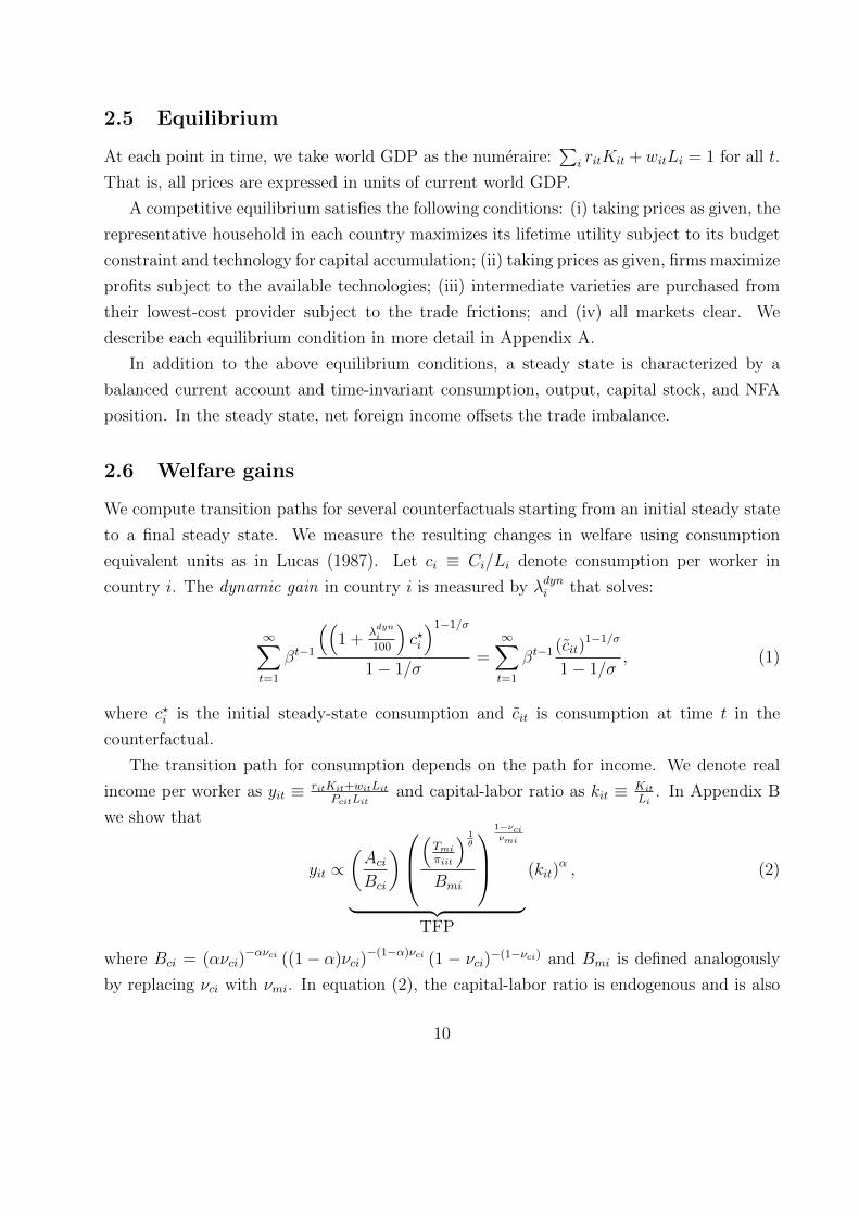
2.6 Welfare gains

We compute transition paths for several counterfactuals starting from an initial steady state

to a final steady state. We measure the resulting changes in welfare using consumption

equivalent units as in Lucas (1987). Let ci ≡ Ci/Li denote consumption per worker in

country i. The dynamic gain in country i is measured by λdyni that solves:

∞∑t=1

βt−1

((1 +

λdyni

100

)c?i

)1−1/σ

1− 1/σ=∞∑t=1

βt−1 (cit)1−1/σ

1− 1/σ, (1)

where c?i is the initial steady-state consumption and cit is consumption at time t in the

counterfactual.

The transition path for consumption depends on the path for income. We denote real

income per worker as yit ≡ ritKit+witLitPcitLit

and capital-labor ratio as kit ≡ KitLi

. In Appendix B

we show that

yit ∝(AciBci

)(Tmiπiit

) 1θ

Bmi

1−νciνmi

︸ ︷︷ ︸TFP

(kit)α , (2)

where Bci = (ανci)−ανci ((1− α)νci)

−(1−α)νci (1 − νci)−(1−νci) and Bmi is defined analogously

by replacing νci with νmi. In equation (2), the capital-labor ratio is endogenous and is also

10

a function of the home trade share.

Channels for the gains from trade Trade liberalization affects the dynamic gain in

our model through two channels.

1. Trade liberalization results in an immediate and permanent drop in the home trade

shares and, hence, higher TFP on impact. The tradables intensity of consumption,

νci, goods governs the responsiveness of TFP to the change in home trade share. The

higher TFP increases GDP and affects the consumption path.

2. Trade liberalization also increases the rate of capital accumulation due to the increase

in TFP and decrease in the relative price of investment. The responsiveness of capital

depends on the tradabales intensity of investment, νxi.

• The increase in TFP yields a higher marginal product of capital (MPK), which

affects capital accumulation and, hence, income and consumption.

• Trade liberalization also reduces the prices of intermediate varieties. If invest-

ment goods production is more tradables-intensive (νxi < νci), the relative price

of investment goods declines, which makes it feasible to allocate a larger share

of income to investment. Hence, the investment rate and capital-output ratio

increase, affecting income and consumption along the transition path.

Dynamics The dynamics are governed by two intertemporal Euler equations associated

with the one-period bond and capital:

cit+1

cit= βσ

(1 + qt+1

Pcit+1/Pcit

)σ(3)

andcit+1

cit= βσ

( rit+1

Pixt+1− Φ2(kit+2, kit+1)

Φ1(kit+1, kit)

)σ (Pxit+1/Pcit+1

Pxit/Pcit

)σ, (4)

11

where Φ1(·, ·) and Φ2(·, ·) denote the first derivatives of the adjustment-cost function with

respect to the first and second arguments, respectively:

Φ1(k′, k) =

(1

χ

) 1λ(

1

λ

)(k′

k− (1− δ)

) 1−λλ

Φ2(k′, k) =

(1

χ

) 1λ(

1

λ

)(k′

k− (1− δ)

) 1−λλ(

(λ− 1)k′

k− λ(1− δ)

),

where the prime notation denotes the next period’s value.

The dynamics are pinned down by the solution to a system of I simultaneous, second-

order, nonlinear difference equations. Note that the dynamics of capital in country i depend

on the capital stocks in all other countries due to trade. The Euler equations also reveal

that a change in trade friction for any country at any point in time affects the dynamic path

of all countries.

3 Calibration

We calibrate the parameters of our model to match several observations in 2014. We assume

that the world is in steady state in 2014. Our data cover 44 countries (more precisely, 43

countries plus a rest-of-the-world aggregate). Table C.1 in Appendix C provides a list of the

countries. The primary data sources include version 9.0 of the Penn World Table (PWT)

(Feenstra, Inklaar, and Timmer, 2015) and the World Input-Output Database (WIOD)

(Timmer, Dietzenbacher, Los, and de Vries, 2015; Timmer, Los, Stehrer, and de Vries,

2016). More details about the data are provided in Appendix C.

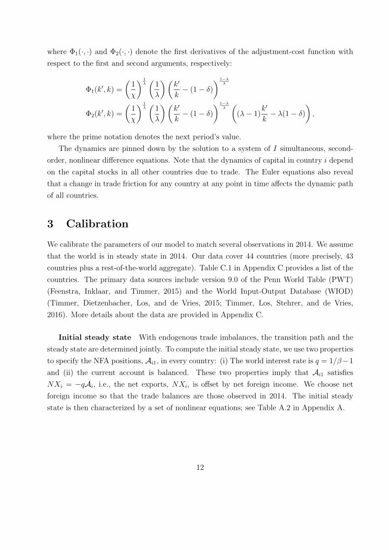
Initial steady state With endogenous trade imbalances, the transition path and the

steady state are determined jointly. To compute the initial steady state, we use two properties

to specify the NFA positions, Ai1, in every country: (i) The world interest rate is q = 1/β−1

and (ii) the current account is balanced. These two properties imply that Ai1 satisfies

NXi = −qAi, i.e., the net exports, NXi, is offset by net foreign income. We choose net

foreign income so that the trade balances are those observed in 2014. The initial steady

state is then characterized by a set of nonlinear equations; see Table A.2 in Appendix A.

12

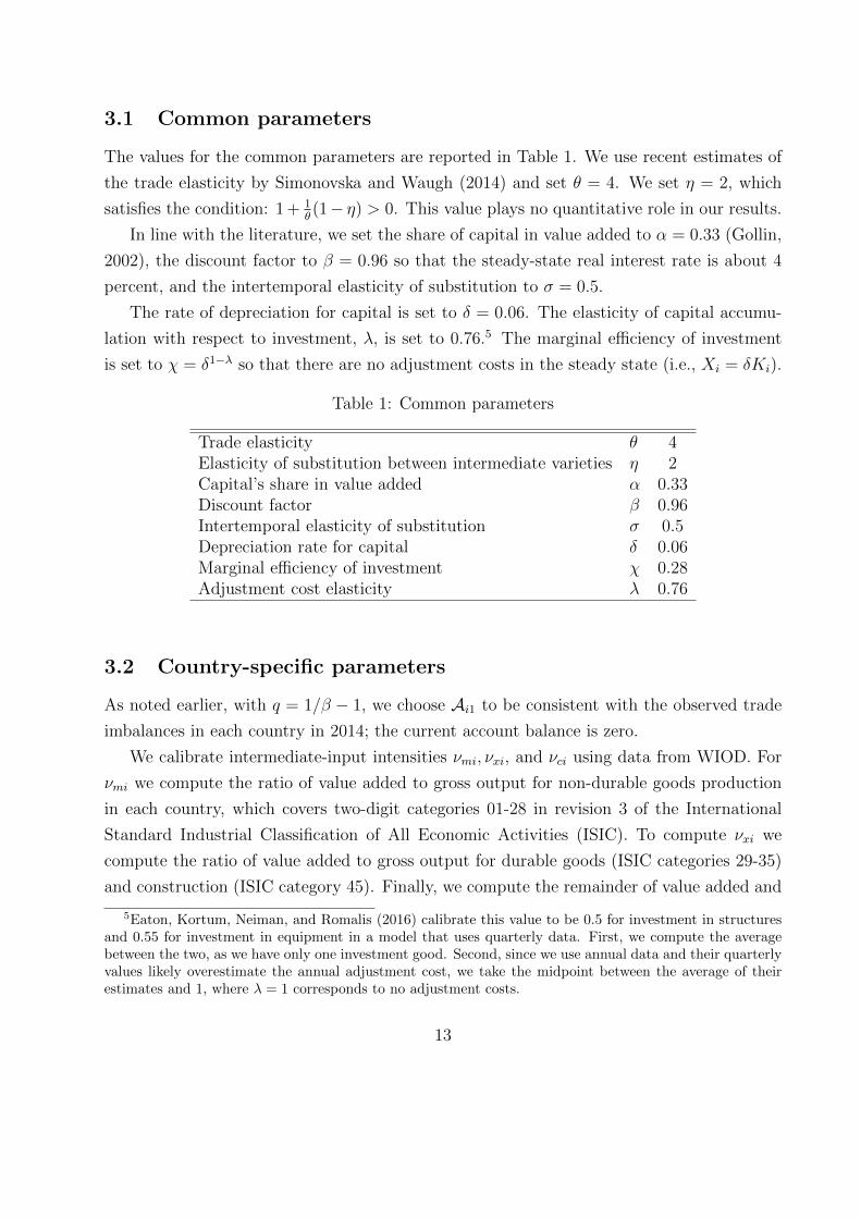
3.1 Common parameters

The values for the common parameters are reported in Table 1. We use recent estimates of

the trade elasticity by Simonovska and Waugh (2014) and set θ = 4. We set η = 2, which

satisfies the condition: 1 + 1θ(1− η) > 0. This value plays no quantitative role in our results.

In line with the literature, we set the share of capital in value added to α = 0.33 (Gollin,

2002), the discount factor to β = 0.96 so that the steady-state real interest rate is about 4

percent, and the intertemporal elasticity of substitution to σ = 0.5.

The rate of depreciation for capital is set to δ = 0.06. The elasticity of capital accumu-

lation with respect to investment, λ, is set to 0.76.5 The marginal efficiency of investment

is set to χ = δ1−λ so that there are no adjustment costs in the steady state (i.e., Xi = δKi).

Table 1: Common parameters

Trade elasticity θ 4Elasticity of substitution between intermediate varieties η 2Capital’s share in value added α 0.33Discount factor β 0.96Intertemporal elasticity of substitution σ 0.5Depreciation rate for capital δ 0.06Marginal efficiency of investment χ 0.28Adjustment cost elasticity λ 0.76

3.2 Country-specific parameters

As noted earlier, with q = 1/β − 1, we choose Ai1 to be consistent with the observed trade

imbalances in each country in 2014; the current account balance is zero.

We calibrate intermediate-input intensities νmi, νxi, and νci using data from WIOD. For

νmi we compute the ratio of value added to gross output for non-durable goods production

in each country, which covers two-digit categories 01-28 in revision 3 of the International

Standard Industrial Classification of All Economic Activities (ISIC). To compute νxi we

compute the ratio of value added to gross output for durable goods (ISIC categories 29-35)

and construction (ISIC category 45). Finally, we compute the remainder of value added and

5Eaton, Kortum, Neiman, and Romalis (2016) calibrate this value to be 0.5 for investment in structuresand 0.55 for investment in equipment in a model that uses quarterly data. First, we compute the averagebetween the two, as we have only one investment good. Second, since we use annual data and their quarterlyvalues likely overestimate the annual adjustment cost, we take the midpoint between the average of theirestimates and 1, where λ = 1 corresponds to no adjustment costs.

13

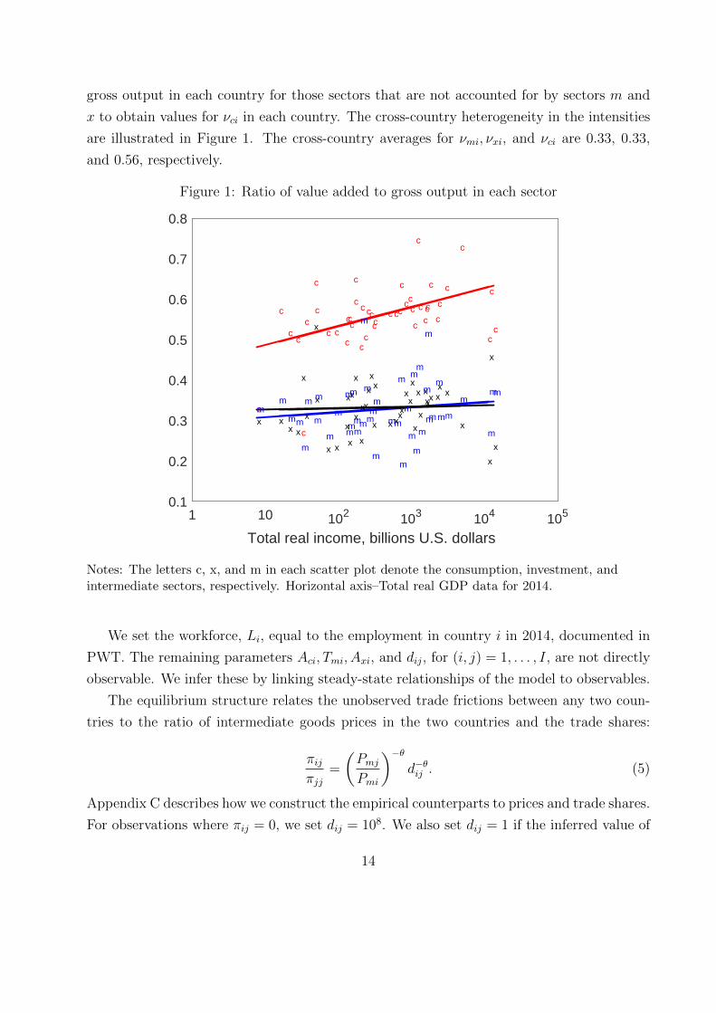
gross output in each country for those sectors that are not accounted for by sectors m and

x to obtain values for νci in each country. The cross-country heterogeneity in the intensities

are illustrated in Figure 1. The cross-country averages for νmi, νxi, and νci are 0.33, 0.33,

and 0.56, respectively.

Figure 1: Ratio of value added to gross output in each sector

1 10 102 103 104 105

Total real income, billions U.S. dollars

0.1

0.2

0.3

0.4

0.5

0.6

0.7

0.8

cc

cc

c

cc

c

c

c

c

c

c

c

cc

c

c

cc

c

c

c

c

c

c

c

c

c

c

c

cc

cc

cc

c

cc

cc

cc

m

m

m

m

m

m

m

m

m

mm

m

m

m

mm

m

m

m

m

m

mm

m

m

m

m

m

m

m

mm

m

mm

m mm

mm

m m

m

m

x

x

x

x

x

xx

x

x

x

xx

x

x

xxx

x

x

x

x

xxx

x

x

x

x

x

x

x x

x

xxx

x

x

x

x

x

x

x

x

Notes: The letters c, x, and m in each scatter plot denote the consumption, investment, andintermediate sectors, respectively. Horizontal axis–Total real GDP data for 2014.

We set the workforce, Li, equal to the employment in country i in 2014, documented in

PWT. The remaining parameters Aci, Tmi, Axi, and dij, for (i, j) = 1, . . . , I, are not directly

observable. We infer these by linking steady-state relationships of the model to observables.

The equilibrium structure relates the unobserved trade frictions between any two coun-

tries to the ratio of intermediate goods prices in the two countries and the trade shares:

πijπjj

=

(PmjPmi

)−θd−θij . (5)

Appendix C describes how we construct the empirical counterparts to prices and trade shares.

For observations where πij = 0, we set dij = 108. We also set dij = 1 if the inferred value of

14

trade cost is less than 1.

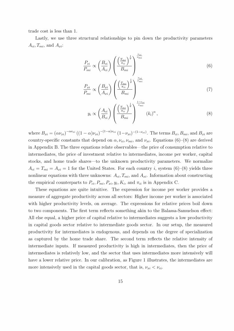
Lastly, we use three structural relationships to pin down the productivity parameters

Aci, Tmi, and Axi:

PciPmi∝(Bci

Aci

)(Tmiπii

) 1θ

Bmi

νciνmi

(6)

PxiPmi∝(Bxi

Axi

)(Tmiπii

) 1θ

Bmi

νxiνmi

(7)

yi ∝(AciBci

)(Tmiπii

) 1θ

Bmi

1−νciνmi

(ki)α , (8)

where Bxi = (ανxi)−ανxi ((1− α)νxi)

−(1−α)νxi (1−νxi)−(1−νxi). The terms Bci, Bmi, and Bxi are

country-specific constants that depend on α, νci, νmi, and νxi. Equations (6)–(8) are derived

in Appendix B. The three equations relate observables—the price of consumption relative to

intermediates, the price of investment relative to intermediates, income per worker, capital

stocks, and home trade shares—to the unknown productivity parameters. We normalize

Aci = Tmi = Axi = 1 for the United States. For each country i, system (6)–(8) yields three

nonlinear equations with three unknowns: Aci, Tmi, and Axi. Information about constructing

the empirical counterparts to Pci, Pmi, Pxi, yi, Ki, and πii is in Appendix C.

These equations are quite intuitive. The expression for income per worker provides a

measure of aggregate productivity across all sectors: Higher income per worker is associated

with higher productivity levels, on average. The expressions for relative prices boil down

to two components. The first term reflects something akin to the Balassa-Samuelson effect:

All else equal, a higher price of capital relative to intermediates suggests a low productivity

in capital goods sector relative to intermediate goods sector. In our setup, the measured

productivity for intermediates is endogenous, and depends on the degree of specialization

as captured by the home trade share. The second term reflects the relative intensity of

intermediate inputs. If measured productivity is high in intermediates, then the price of

intermediates is relatively low, and the sector that uses intermediates more intensively will

have a lower relative price. In our calibration, as Figure 1 illustrates, the intermediates are

more intensively used in the capital goods sector, that is, νxi < νci.

15

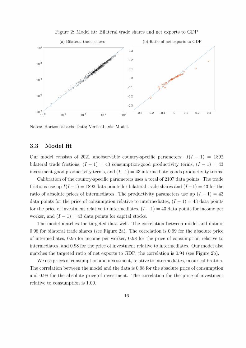
Figure 2: Model fit: Bilateral trade shares and net exports to GDP

(a) Bilateral trade shares

10-8 10-6 10-4 10-2 10010-8

10-6

10-4

10-2

100

.

..

..

.

.

.

.. ..

. . .

.

...

..

..

..

.

.

.

. .

..

.

..

.

..

...

.

..

.

.

..

.

.

.

..

..

.. .

..

..

..

.

.

..

. ..

.

...

.

.

.

..

.

.

..

. .

.

..

. .

.

.

...

..

..

..

..

.

. .

..

..

.

.

.

.

.

.

. ...

..

. ..

.

..

.

..

.

.

.

.

.

..

....

..

.

..

.

.

..

.

.

.

.

.

.

.

.

.

..

.

..

..

.

.

. .

..

.

..

...

.

.. ..

...

...

.

.

....

.

.

.. .

..

.

.

.

.

.

.

.

..

...

.

..

. ....

..

...

.

.

..

.

..

.

..

.

. ..

...

.

.. .

.

.

.

.

..

.

.

.

.

..

.

.

.

..

.

.....

....

.

.

..

..

. .

.

..

....... .

.

....

.

.

..

..

.

..

... ...

....

.

. ....

.

.

....

....

..

.

...

..

.

..

.

.

.

.

.

.

. .

.

.

..

.

.

..

. .

..

.

.

.

.

.

.

.

...

.

.

.

.

.

.

.

.

.

.

.

.

..

..

.

.

.

..

.

.

....

.

.

.

.

..

..

.

.

.

.

.

..

.

.

.

.

.

.

.

.

.

..

.

.

..

. .

.

.

.

..

.

.....

..

. .

..

..

.

.

.

.

.

.

.

.

. .

.

.

...

.

..

. . ..

..

.

.

...

.

..

...

.

.

.

.

.

...

.

.

.

.

..

.

..

...

..

.

.. .

.

..

.

..

.

.

.

.....

.

.

.

..

..

..

..

...

.

..

. .

.

....

.

..

.

.

..

..

.

.

.

.

.. .

.

.

.

. ...

.

.

.

.

..

.

.

.

.

.

.

.

.

.

...

.

..

.

.

..

..

.

.

.

..

.

...

.

.

.

..

..

.

..

.

.

..

.

.

.

. .

..

.

...

.

..

.

.

..

.

.

.

.

. .

.

.

.. .. .

....

.

.

..

..

..

.

.

.

.

..

...

...

.. ..

..

..

.

.

.

.

.

.

.

..

.... ..

.

.

.

.

.

.

.

.

...

.

...

...

....

.

.

..

.

..

.

.

..

.

.

....

....

.

.

.

.

.

.

.

..

.

.

.

.

.

.

..

.

.

.

.

.

.

.

.

..

.

.

.

.

.

.

.

..

..

...

..

.

.

.

.

.

.

.

.

...

.

.

.. .

.

..

.

.

.

.

.

.

.

.

.

.

.

..

.

.

.

.

..

.

.

....

.

..

..

..

.

.

.

.

..

.

.

.

.

..

..

..

. .

.

.

.. ..

.

..

.

...

.

....

.

.

.

..

..

..

...

.

. . ..

.

.

.

.

.

.

.

.

.

.

..

...

.

... .... .

..

.

.

...

..

.

.

..

..

. ..

.

.

..

..

..

.. .

.

.

.

.

.

.

...

.

..

..

.

.

..

..

.

..

.

..

.

..

...

... ..

.

..

.

.

.. .

..

.

.

...

....

..

..

.

. .

.

..

...

.

.

..

. ..

..

.

.

..

..

.

.

.

.

.. ..

.

...

.

.. ..

..

.

.

. .

.

.

...

.

...

...

.

..

...

.

.

.

.

.

. . .

.

.

.

....

.

..

....

.

.

..

..

.

.

..

.

.

.. .

..

..

.

.

.

.

.

.

..

.

..

.

.

..

.

.

.

.

..

..

.

.

.

.

.

..

.

.

.

.

...

..

.

.

. .

.

.

.

.

.

.

.

.

.

.

.

.

.

..

.

...

.

...

.

..

.

.

..

..

.

.

.

..

...

... .

.

..

.

..

.

.

.

.

.

...

.

.

.

.

.

.

..

.

.

.

.

.

.

.

.

.

.

..

.

.

. ..

.

..

.

.

.

.

.

.

.

.

.

.

.

..

...

.

..

. .

.

.

.

.

.

.

....

...

.

....

.

.

..

.

..

.

.

.

..

.

..

.

.

...

.

..

..

...

..

..

..

.

...

.

.

..

..

..

. .

.

.

.

.

.

.

.

. .

.

.

..

..

..

......

..

.

.

. .

. ..

.

....

...

..

.

.

..

.

.

.

.

..

.

.

..

.

.

..

.

.

.

.

....

.

...

.

.

.

.

.

..

.

.

..

..

.

.

...

..

.

.

.

.

.

.

.

..

.

.

....

.

.

..

..

..

.

.

.

.

.

..

.

.

.

.

.

..

.

...

.

..

..

.

.

.. ..

.

. ..

..

.

.

..

.

.

..

..

..

..

....

...

..

..

.

.

.

.

.

..

.

......

.

..

..

.

..

.

.

..

...

.

..

.

...

.

..

.

.

..

.

..

.....

.

...

..

...

.....

... .

.

.

.

.

..

. .

... ..

.

. .

.

.

...

.

.

.

.

..

...

..

. ..

..

..

..

..

.

.

.

.

...

.

.

.. .

.

..

.

.

.

.

.

.

..

.

.

.

.

.

.

.

..

...

.

.

.

.

..

.

.

.

.

.

.

...

.

.

.

..

.

..

..

.

.

.

.

.

.

.

.

.

..

.

.

.

. ..

.

.

.

.

.

.

.

..

.

.

.

.

...

.

.

.

..

.

..

..

.

..

.

..

.

.

.. .

.

.

..

..

..

.

..

.

.

..

.

.

.

.

..

.

..

...

...

..

.

. .

.

..

.

..

..

...

..

.

...

.

.

..

..

.

.

.

.

.

.

..

.

.. .

...

..

.

..

.

. .

.

.

.. ...

.

..

...

.

.

.

..

..

...

.

.

....

.

.

..

...

.

.

.

.

.

.

.

.

. ..

.. .

..

..

.

...

.

.

...

..

.

.

..

.

. ..

.

.

....

.

(b) Ratio of net exports to GDP

-0.3 -0.2 -0.1 0 0.1 0.2 0.3

-0.3

-0.2

-0.1

0

0.1

0.2

0.3

Notes: Horizontal axis–Data; Vertical axis–Model.

3.3 Model fit

Our model consists of 2021 unobservable country-specific parameters: I(I − 1) = 1892

bilateral trade frictions, (I − 1) = 43 consumption-good productivity terms, (I − 1) = 43

investment-good productivity terms, and (I−1) = 43 intermediate-goods productivity terms.

Calibration of the country-specific parameters uses a total of 2107 data points. The trade

frictions use up I(I−1) = 1892 data points for bilateral trade shares and (I−1) = 43 for the

ratio of absolute prices of intermediates. The productivity parameters use up (I − 1) = 43

data points for the price of consumption relative to intermediates, (I − 1) = 43 data points

for the price of investment relative to intermediates, (I − 1) = 43 data points for income per

worker, and (I − 1) = 43 data points for capital stocks.

The model matches the targeted data well. The correlation between model and data is

0.98 for bilateral trade shares (see Figure 2a). The correlation is 0.99 for the absolute price

of intermediates, 0.95 for income per worker, 0.98 for the price of consumption relative to

intermediates, and 0.98 for the price of investment relative to intermediates. Our model also

matches the targeted ratio of net exports to GDP; the correlation is 0.94 (see Figure 2b).

We use prices of consumption and investment, relative to intermediates, in our calibration.

The correlation between the model and the data is 0.98 for the absolute price of consumption

and 0.98 for the absolute price of investment. The correlation for the price of investment

relative to consumption is 1.00.

16

Untargeted moments The correlation between the model and the data on capital-

labor ratios is 0.71. In both the model and the data, the nominal investment rate is uncor-

related with the level of income per worker. The cross-country average nominal investment

rate, PxXwL+rK

, is 17.4 percent in the model and is 23.3 percent in the data.

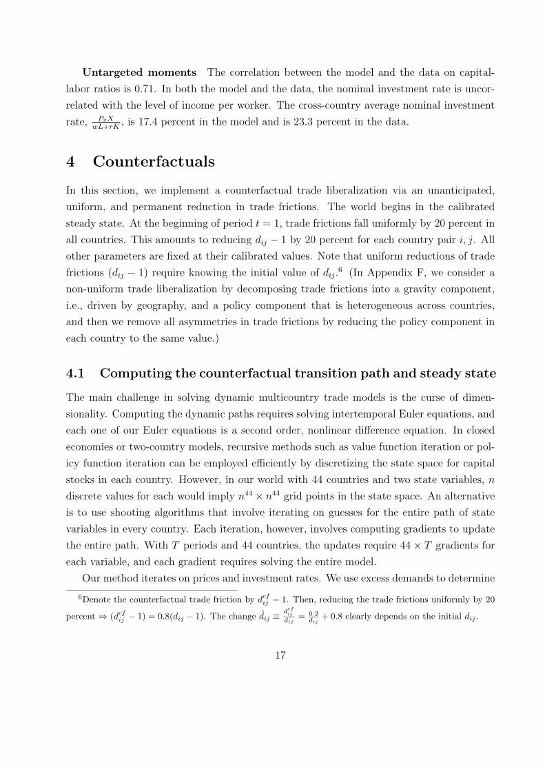
4 Counterfactuals

In this section, we implement a counterfactual trade liberalization via an unanticipated,

uniform, and permanent reduction in trade frictions. The world begins in the calibrated

steady state. At the beginning of period t = 1, trade frictions fall uniformly by 20 percent in

all countries. This amounts to reducing dij − 1 by 20 percent for each country pair i, j. All

other parameters are fixed at their calibrated values. Note that uniform reductions of trade

frictions (dij − 1) require knowing the initial value of dij.6 (In Appendix F, we consider a

non-uniform trade liberalization by decomposing trade frictions into a gravity component,

i.e., driven by geography, and a policy component that is heterogeneous across countries,

and then we remove all asymmetries in trade frictions by reducing the policy component in

each country to the same value.)

4.1 Computing the counterfactual transition path and steady state

The main challenge in solving dynamic multicountry trade models is the curse of dimen-

sionality. Computing the dynamic paths requires solving intertemporal Euler equations, and

each one of our Euler equations is a second order, nonlinear difference equation. In closed

economies or two-country models, recursive methods such as value function iteration or pol-

icy function iteration can be employed efficiently by discretizing the state space for capital

stocks in each country. However, in our world with 44 countries and two state variables, n

discrete values for each would imply n44 × n44 grid points in the state space. An alternative

is to use shooting algorithms that involve iterating on guesses for the entire path of state

variables in every country. Each iteration, however, involves computing gradients to update

the entire path. With T periods and 44 countries, the updates require 44× T gradients for

each variable, and each gradient requires solving the entire model.

Our method iterates on prices and investment rates. We use excess demands to determine

6Denote the counterfactual trade friction by dcfij − 1. Then, reducing the trade frictions uniformly by 20

percent ⇒ (dcfij − 1) = 0.8(dij − 1). The change dij ≡dcfij

dij= 0.2

dij+ 0.8 clearly depends on the initial dij .

17

the size and direction of the change in prices and investment rates in each iteration. We

bypass the costly computation of gradients and compute the entire transition path in less

than two hours on a standard computer.

To compute the counterfactual transition path and the counterfactual steady state, we

first reduce the infinite horizon problem to a finite horizon model with t = 1, . . . , T periods.

We make T sufficiently large to ensure convergence to a new steady state; T = 150 proved

sufficient in our computations.

We start with a guess: The terminal NFA position AiT+1 = 0, for all i. We then guess the

entire sequences of nominal investment rates, ρit = PxitXitwitLit+ritKit

, and wages for every country,

as well as one sequence of world interest rates. Taking the nominal investment rate as given,

we iterate over wages and the world interest rate using excess demand equations. The wages

and the world interest rate help us recover all other prices and trade shares from first-order

conditions and a subset of market-clearing conditions. We use deviations from the balance

of payments identity—net purchases of bonds equals net exports plus net foreign income—

and trade balance at the world level to update the sequences of wages in every country and

the world interest rate simultaneously. We repeat the process until we find sequences that

satisfy the balance of payments. With these sequences, we check whether the Euler equation

for investment in capital is satisfied. We use deviations from the Euler equation to update

the nominal investment rate in every country at every point in time simultaneously. Using

the transition path of the NFA position, we update the terminal AiT+1 by setting it to Aitwhere t is some period close to but less than T . We continue this procedure until we reach a

fixed point in the sequence of nominal investment rates and the steady-state NFA position.

Appendix D describes our solution method in more detail. Our method is also valid for

the environment with the complete IO structure (Appendix G) and for non-uniform trade

liberalizations (Appendix F).

The presence of both capital and bonds introduces a challenge in computing transitional

dynamics. To see why, consider a model with one-period bonds but no capital accumula-

tion, as in Reyes-Heroles (2016). In his environment, the counterfactual NFA position is

indeterminate, so to solve the model one must choose an ad-hoc terminal NFA position.

Different terminal NFA positions give rise to different dynamics in consumption and net

exports, thereby affecting the welfare implications. In our model with capital, the counter-

factual terminal NFA position is uniquely pinned down because of (i) diminishing returns to

capital accumulation and (ii) the real rates of return on capital and bonds must be equal in

each country at every point in time. As a result, current accounts respond in order to equal-

18

ize rates of return across countries and the counterfactual steady state must be determined

jointly with the entire transition path, making the computation challenging. Furthermore,

the number of periods it takes for our economy to reach its counterfactual steady state and,

hence, half-life is endogenous. Put differently, with ad-hoc terminal NFA positions the period

when the economy reaches the counterfactual steady state is also ad-hoc.

Eaton, Kortum, Neiman, and Romalis (2016) use the “hat algebra” approach to solve

for changes in endogenous variables; Zylkin (2016) uses a similar approach to study the

dynamic effects of China’s integration into the world economy. The computation of the

counterfactual in these papers can proceed without knowing the initial trade frictions. For

the types of counterfactual exercises such as ours, one needs to know the initial level of

trade frictions (see example in footnote 6). Conditional on knowing them, the hat algebra

approach is essentially equivalent to ours. However, in contrast to the algorithms in these

papers, our algorithm is gradient-free and, therefore, more efficient.7

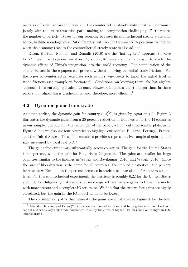
4.2 Dynamic gains from trade

As noted earlier, the dynamic gain for country i, λdyni , is given by equation (1). Figure 3

illustrates the dynamic gains from a 20 percent reduction in trade costs for the 44 countries

in our sample. Throughout the remainder of the paper, we not only use scatter plots, as in

Figure 3, but we also use four countries to highlight our results: Bulgaria, Portugal, France,

and the United States. These four countries provide a representative sample of gains and of

size, measured by total real GDP.

The gains from trade vary substantially across countries: The gain for the United States

is 4.4 percent, while the gain for Bulgaria is 21 percent. The gains are smaller for large

countries, similar to the findings in Waugh and Ravikumar (2016) and Waugh (2010). Since

the size of liberalization is the same for all countries, the implied elasticities—the percent

increase in welfare due to the percent decrease in trade cost—are also different across coun-

tries. For this counterfactual experiment, the elasticity is roughly 0.22 for the United States

and 1.06 for Bulgaria. (In Appendix G, we compare these welfare gains to those in a model

with more sectors and a complete IO structure. We find that the two welfare gains are highly

correlated, but the gain in the IO model tends to be lower.)

The consumption paths that generate the gains are illustrated in Figure 4 for the four

7Caliendo, Dvorkin, and Parro (2017) use excess demand iteration and hat algebra in a model withoutcapital and with exogenous trade imbalances to study the effect of higher TFP in China on changes in U.S.labor markets.

19

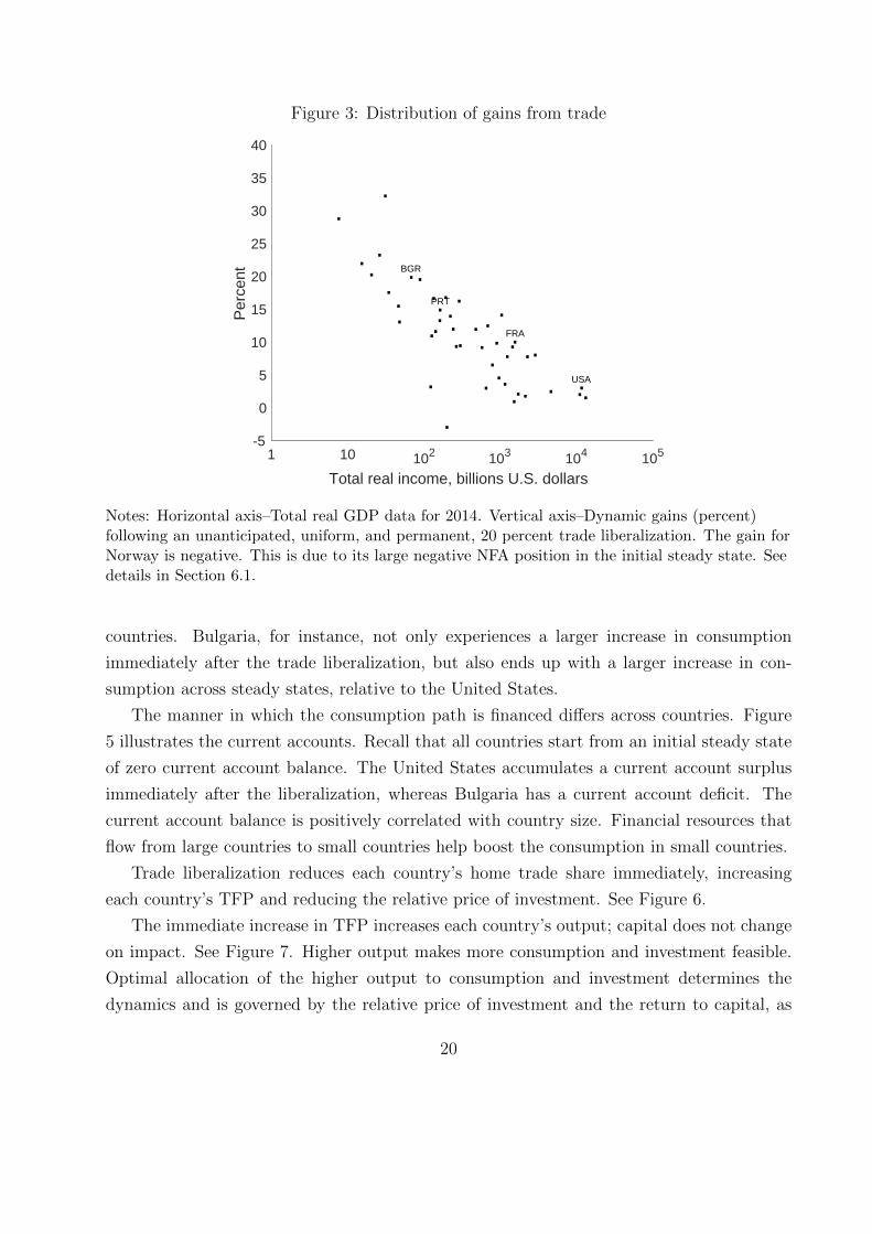
Figure 3: Distribution of gains from trade

1 10 102 103 104 105

Total real income, billions U.S. dollars

-5

0

5

10

15

20

25

30

35

40

Per

cent

.

..

BGR.

...

.

..

.. .

.

. FRA.....

. ... ...

.

.

.

.

.

.

.

PRT. .

..

..

...

USA.

Notes: Horizontal axis–Total real GDP data for 2014. Vertical axis–Dynamic gains (percent)following an unanticipated, uniform, and permanent, 20 percent trade liberalization. The gain forNorway is negative. This is due to its large negative NFA position in the initial steady state. Seedetails in Section 6.1.

countries. Bulgaria, for instance, not only experiences a larger increase in consumption

immediately after the trade liberalization, but also ends up with a larger increase in con-

sumption across steady states, relative to the United States.

The manner in which the consumption path is financed differs across countries. Figure

5 illustrates the current accounts. Recall that all countries start from an initial steady state

of zero current account balance. The United States accumulates a current account surplus

immediately after the liberalization, whereas Bulgaria has a current account deficit. The

current account balance is positively correlated with country size. Financial resources that

flow from large countries to small countries help boost the consumption in small countries.

Trade liberalization reduces each country’s home trade share immediately, increasing

each country’s TFP and reducing the relative price of investment. See Figure 6.

The immediate increase in TFP increases each country’s output; capital does not change

on impact. See Figure 7. Higher output makes more consumption and investment feasible.

Optimal allocation of the higher output to consumption and investment determines the

dynamics and is governed by the relative price of investment and the return to capital, as

20

Figure 4: Transition path for consumption

0 10 20 30 40 50Year

0.95

1

1.05

1.1

1.15

1.2

1.25

1.3BGRPRTFRAUSA

Notes: Transitions following an unanticipated, uniform, and permanent 20 percent tradeliberalization. Initial steady state is normalized to 1. The liberalization occurs in period 1.

revealed by Euler equation (4). Investment increases by more than consumption because

(i) the relative price of investment decreases and (ii) higher TFP causes MPK to increase.

As capital accumulates, output continues to increase. Recall that the increase in output

on impact is entirely due to TFP, whereas the increase in output after the initial period is

driven entirely by capital accumulation.

With a frictionless bond market, MPKs are equalized across countries, and resources flow

to countries that experience a larger increase in TFP. These countries run a current account

deficit in the short run and use it to finance increases in consumption and investment that

exceed increases in output (e.g., Bulgaria, Portugal, and France). In the new steady state the

current account is balanced, but countries that accumulate debt along the transition have

to run trade surpluses to service the debt. In general, small countries run current account

deficits and large countries run current account surpluses in the short run.

Half life The behavior of trade imbalances also reveals a pattern in the rates of capital

accumulation. Figure 8 illustrates that the half-life for capital accumulation—the number

of periods it takes for the capital stock to reach the midpoint between the initial and coun-

21

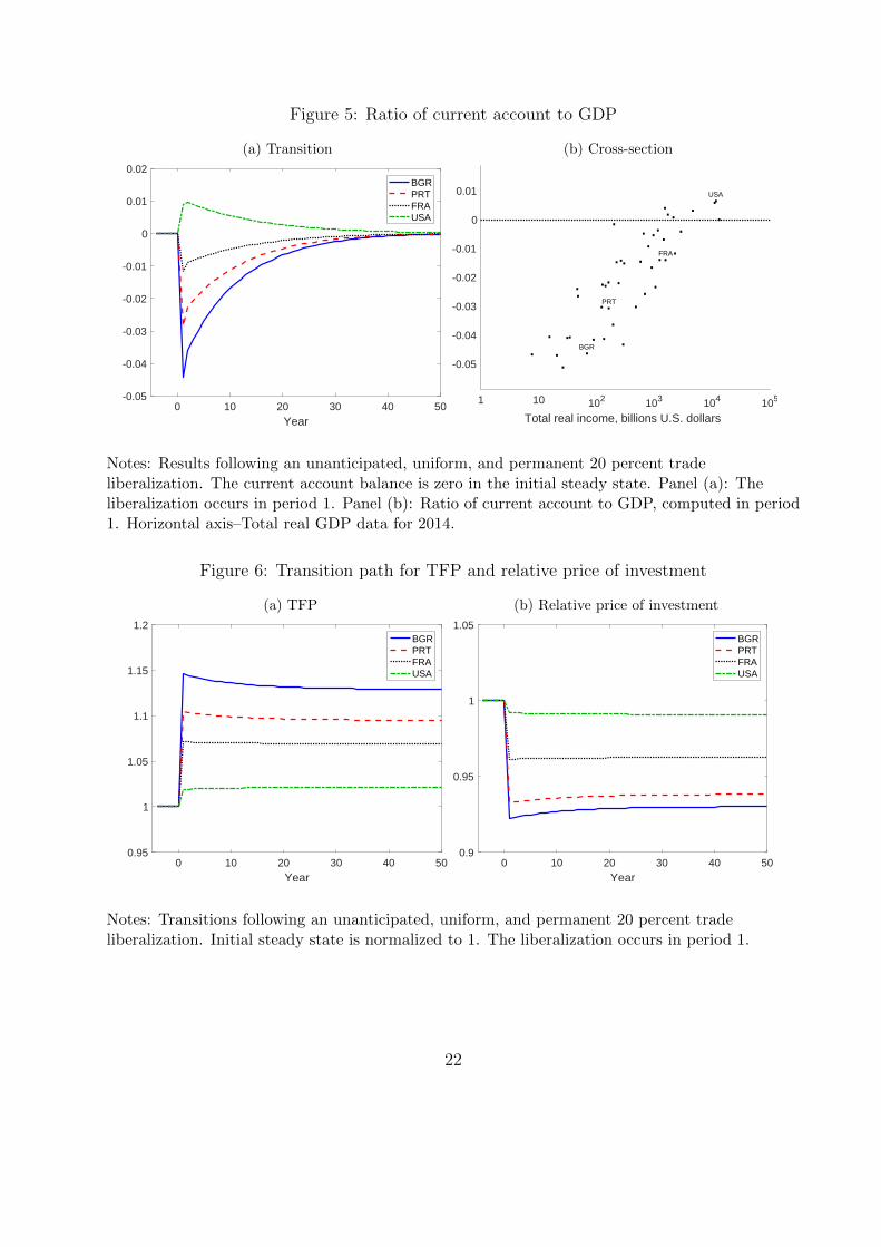
Figure 5: Ratio of current account to GDP

(a) Transition

0 10 20 30 40 50Year

-0.05

-0.04

-0.03

-0.02

-0.01

0

0.01

0.02BGRPRTFRAUSA

(b) Cross-section

1 10 102 103 104 105

Total real income, billions U.S. dollars

-0.05

-0.04

-0.03

-0.02

-0.01

0

0.01

.

.

.BGR.

..

.

.

. .

.

..

.

.FRA..

..

.

. .

.

..

..

..

.

.

.

.

.

PRT.

.

..

..

..

.

USA.

Notes: Results following an unanticipated, uniform, and permanent 20 percent tradeliberalization. The current account balance is zero in the initial steady state. Panel (a): Theliberalization occurs in period 1. Panel (b): Ratio of current account to GDP, computed in period1. Horizontal axis–Total real GDP data for 2014.

Figure 6: Transition path for TFP and relative price of investment

(a) TFP

0 10 20 30 40 50Year

0.95

1

1.05

1.1

1.15

1.2BGRPRTFRAUSA

(b) Relative price of investment

0 10 20 30 40 50Year

0.9

0.95

1

1.05BGRPRTFRAUSA

Notes: Transitions following an unanticipated, uniform, and permanent 20 percent tradeliberalization. Initial steady state is normalized to 1. The liberalization occurs in period 1.

22

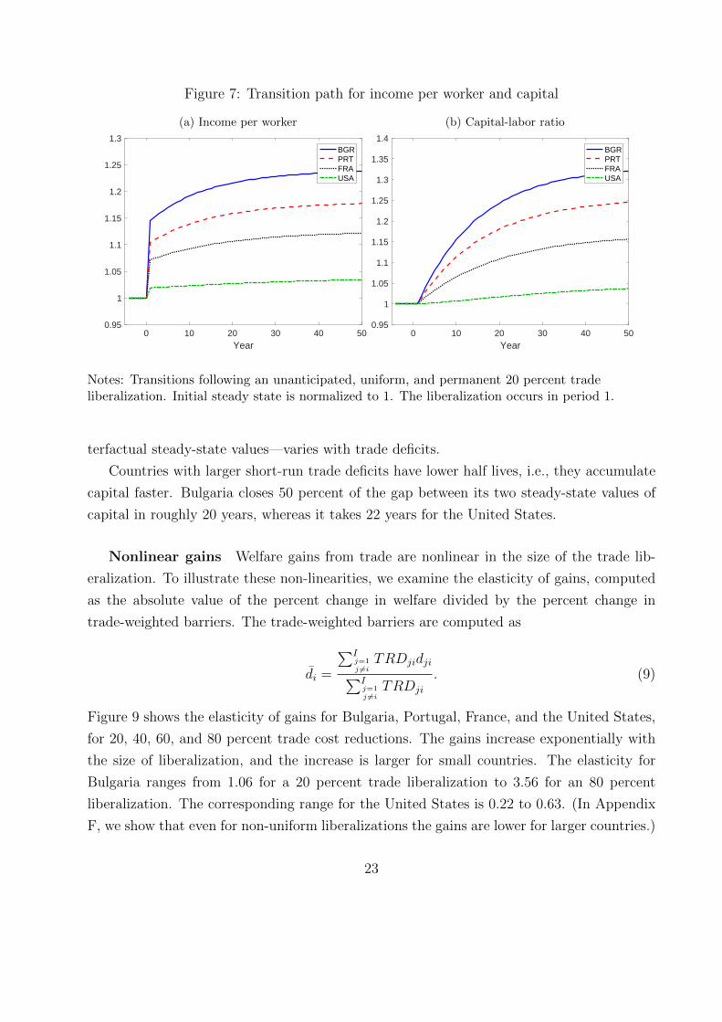
Figure 7: Transition path for income per worker and capital

(a) Income per worker

0 10 20 30 40 50Year

0.95

1

1.05

1.1

1.15

1.2

1.25

1.3BGRPRTFRAUSA

(b) Capital-labor ratio

0 10 20 30 40 50Year

0.95

1

1.05

1.1

1.15

1.2

1.25

1.3

1.35

1.4BGRPRTFRAUSA

Notes: Transitions following an unanticipated, uniform, and permanent 20 percent tradeliberalization. Initial steady state is normalized to 1. The liberalization occurs in period 1.

terfactual steady-state values—varies with trade deficits.

Countries with larger short-run trade deficits have lower half lives, i.e., they accumulate

capital faster. Bulgaria closes 50 percent of the gap between its two steady-state values of

capital in roughly 20 years, whereas it takes 22 years for the United States.

Nonlinear gains Welfare gains from trade are nonlinear in the size of the trade lib-

eralization. To illustrate these non-linearities, we examine the elasticity of gains, computed

as the absolute value of the percent change in welfare divided by the percent change in

trade-weighted barriers. The trade-weighted barriers are computed as

di =

∑Ij=1j 6=i

TRDjidji∑Ij=1j 6=i

TRDji

. (9)

Figure 9 shows the elasticity of gains for Bulgaria, Portugal, France, and the United States,

for 20, 40, 60, and 80 percent trade cost reductions. The gains increase exponentially with

the size of liberalization, and the increase is larger for small countries. The elasticity for

Bulgaria ranges from 1.06 for a 20 percent trade liberalization to 3.56 for an 80 percent

liberalization. The corresponding range for the United States is 0.22 to 0.63. (In Appendix

F, we show that even for non-uniform liberalizations the gains are lower for larger countries.)

23

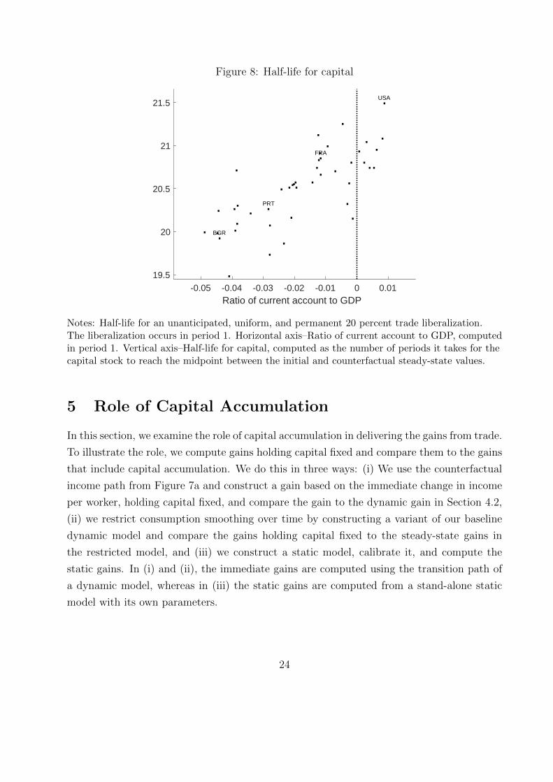
Figure 8: Half-life for capital

-0.05 -0.04 -0.03 -0.02 -0.01 0 0.01Ratio of current account to GDP

19.5

20

20.5

21

21.5

..

.

BGR.

.

.

.

.

. .

.

. .

.

.

FRA.

.

..

.

..

.

..

.

..

...

.

..

PRT.

.

..

..

..

.

USA.

Notes: Half-life for an unanticipated, uniform, and permanent 20 percent trade liberalization.The liberalization occurs in period 1. Horizontal axis–Ratio of current account to GDP, computedin period 1. Vertical axis–Half-life for capital, computed as the number of periods it takes for thecapital stock to reach the midpoint between the initial and counterfactual steady-state values.

5 Role of Capital Accumulation

In this section, we examine the role of capital accumulation in delivering the gains from trade.

To illustrate the role, we compute gains holding capital fixed and compare them to the gains

that include capital accumulation. We do this in three ways: (i) We use the counterfactual

income path from Figure 7a and construct a gain based on the immediate change in income

per worker, holding capital fixed, and compare the gain to the dynamic gain in Section 4.2,

(ii) we restrict consumption smoothing over time by constructing a variant of our baseline

dynamic model and compare the gains holding capital fixed to the steady-state gains in

the restricted model, and (iii) we construct a static model, calibrate it, and compute the

static gains. In (i) and (ii), the immediate gains are computed using the transition path of

a dynamic model, whereas in (iii) the static gains are computed from a stand-alone static

model with its own parameters.

24

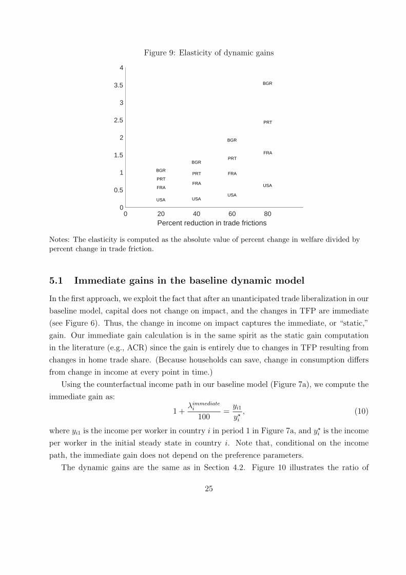
Figure 9: Elasticity of dynamic gains

0 20 40 60 80Percent reduction in trade frictions

0

0.5

1

1.5

2

2.5

3

3.5

4

BGR

PRT

FRA

USA

BGR

PRT

FRA

USA

BGR

PRT

FRA

USA

BGR

PRT

FRA

USA

Notes: The elasticity is computed as the absolute value of percent change in welfare divided bypercent change in trade friction.

5.1 Immediate gains in the baseline dynamic model

In the first approach, we exploit the fact that after an unanticipated trade liberalization in our

baseline model, capital does not change on impact, and the changes in TFP are immediate

(see Figure 6). Thus, the change in income on impact captures the immediate, or “static,”

gain. Our immediate gain calculation is in the same spirit as the static gain computation

in the literature (e.g., ACR) since the gain is entirely due to changes in TFP resulting from

changes in home trade share. (Because households can save, change in consumption differs

from change in income at every point in time.)

Using the counterfactual income path in our baseline model (Figure 7a), we compute the

immediate gain as:

1 +λimmediatei

100=yi1y?i, (10)

where yi1 is the income per worker in country i in period 1 in Figure 7a, and y?i is the income

per worker in the initial steady state in country i. Note that, conditional on the income

path, the immediate gain does not depend on the preference parameters.

The dynamic gains are the same as in Section 4.2. Figure 10 illustrates the ratio of

25

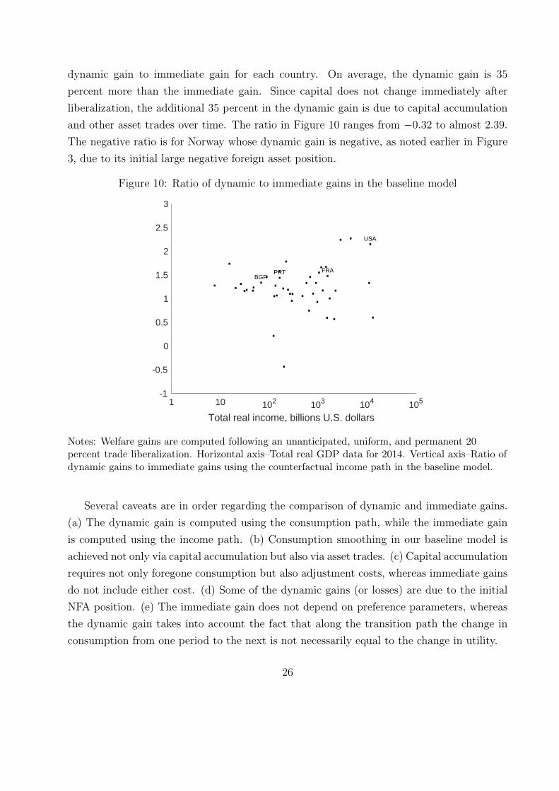
dynamic gain to immediate gain for each country. On average, the dynamic gain is 35

percent more than the immediate gain. Since capital does not change immediately after

liberalization, the additional 35 percent in the dynamic gain is due to capital accumulation

and other asset trades over time. The ratio in Figure 10 ranges from −0.32 to almost 2.39.

The negative ratio is for Norway whose dynamic gain is negative, as noted earlier in Figure

3, due to its initial large negative foreign asset position.

Figure 10: Ratio of dynamic to immediate gains in the baseline model

1 10 102 103 104 105

Total real income, billions U.S. dollars

-1

-0.5

0

0.5

1

1.5

2

2.5

3

...

BGR....

..

. .... .

FRA.... .

.

.

.

.

.

....

..

.

.

.PRT..

..

.. . .

.

USA.

Notes: Welfare gains are computed following an unanticipated, uniform, and permanent 20percent trade liberalization. Horizontal axis–Total real GDP data for 2014. Vertical axis–Ratio ofdynamic gains to immediate gains using the counterfactual income path in the baseline model.

Several caveats are in order regarding the comparison of dynamic and immediate gains.

(a) The dynamic gain is computed using the consumption path, while the immediate gain

is computed using the income path. (b) Consumption smoothing in our baseline model is

achieved not only via capital accumulation but also via asset trades. (c) Capital accumulation

requires not only foregone consumption but also adjustment costs, whereas immediate gains

do not include either cost. (d) Some of the dynamic gains (or losses) are due to the initial

NFA position. (e) The immediate gain does not depend on preference parameters, whereas

the dynamic gain takes into account the fact that along the transition path the change in

consumption from one period to the next is not necessarily equal to the change in utility.

26

In the next subsection, we construct a variant of our baseline model in Section 2 by

imposing restrictions on cross-country trade that help us address the caveats above and

assess the quantitative role of capital accumulation.

5.2 Immediate gains in a restricted dynamic model

We study a variant of our baseline model: We impose balanced trade in the initial steady

state and in each period in the counterfactual; calibrate the variant; and compute the coun-

terfactual transition path. We will refer to this variant as the “restricted dynamic model.”

Balanced trade in the initial steady state eliminates the dependence of gains on initial

trade surpluses or deficits. Balanced trade in every period allows for capital in each country

to be accumulated over time, but it prevents consumption smoothing via asset trades across

countries, helping us isolate the role of capital accumulation. In the restricted dynamic

model, income is proportional to consumption in steady state. Using the welfare gain formula

in equation (1), it is easy to see that the steady-state gains can be measured using changes

in income across steady states:

1 +λssi100

=y??iy?i, (11)

where λssi is the steady-state gain and y??i is the income per worker in the counterfactual

steady state in country i. Thus, both the immediate gain in (10) and the steady-state gain

in (11) use only income and do not depend on the preference parameters and, hence, are

comparable. We can also compare the steady-state cost of autarky to the immediate cost

of autarky using income. (In our baseline model with trade imbalances, we cannot measure

“steady-state” gain or loss via change in consumption or via change in income.)

The only difference in the initial steady state between the restricted dynamic model and

our baseline model in Section 2 is that each country’s trade balance and NFA position are

both zero in the restricted dynamic model. The country-specific parameters inferred from

the structural relationships (5)–(8) do not depend on the country’s trade deficit or the NFA

position. Thus, the parameters for the restricted dynamic model are the same as the ones

for the baseline in Section 3.

We conduct a 20 percent unanticipated, uniform, and permanent trade liberalization in

the restricted dynamic model. Similar to the previous subsection, we use the counterfactual

transition path for income per worker in the restricted dynamic model (Figure 11) to compute

the immediate gain; the formula for the immediate gain is the same as in equation (10)

27

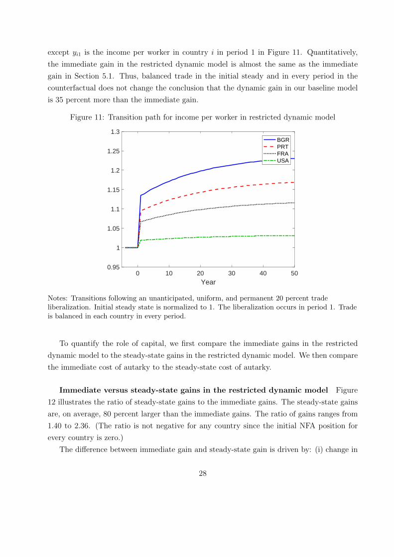
except yi1 is the income per worker in country i in period 1 in Figure 11. Quantitatively,

the immediate gain in the restricted dynamic model is almost the same as the immediate

gain in Section 5.1. Thus, balanced trade in the initial steady and in every period in the

counterfactual does not change the conclusion that the dynamic gain in our baseline model

is 35 percent more than the immediate gain.

Figure 11: Transition path for income per worker in restricted dynamic model

0 10 20 30 40 50Year

0.95

1

1.05

1.1

1.15

1.2

1.25

1.3BGRPRTFRAUSA

Notes: Transitions following an unanticipated, uniform, and permanent 20 percent tradeliberalization. Initial steady state is normalized to 1. The liberalization occurs in period 1. Tradeis balanced in each country in every period.

To quantify the role of capital, we first compare the immediate gains in the restricted

dynamic model to the steady-state gains in the restricted dynamic model. We then compare

the immediate cost of autarky to the steady-state cost of autarky.

Immediate versus steady-state gains in the restricted dynamic model Figure

12 illustrates the ratio of steady-state gains to the immediate gains. The steady-state gains

are, on average, 80 percent larger than the immediate gains. The ratio of gains ranges from

1.40 to 2.36. (The ratio is not negative for any country since the initial NFA position for

every country is zero.)

The difference between immediate gain and steady-state gain is driven by: (i) change in

28

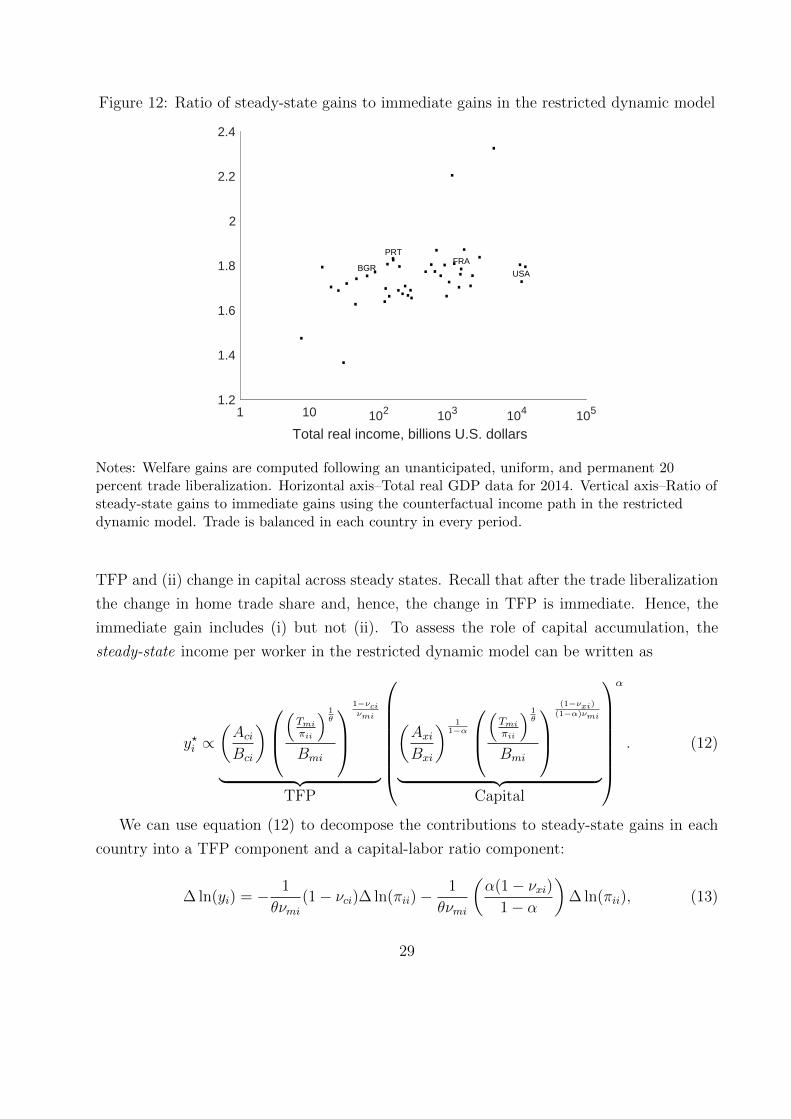
Figure 12: Ratio of steady-state gains to immediate gains in the restricted dynamic model

1 10 102 103 104 105

Total real income, billions U.S. dollars

1.2

1.4

1.6

1.8

2

2.2

2.4

...BGR.

.

....

. ..

.. .

FRA..

.. . .

.

.

. ..

.

.

.

.

.

.. .PRT..

.... .

..

USA.

Notes: Welfare gains are computed following an unanticipated, uniform, and permanent 20percent trade liberalization. Horizontal axis–Total real GDP data for 2014. Vertical axis–Ratio ofsteady-state gains to immediate gains using the counterfactual income path in the restricteddynamic model. Trade is balanced in each country in every period.

TFP and (ii) change in capital across steady states. Recall that after the trade liberalization

the change in home trade share and, hence, the change in TFP is immediate. Hence, the

immediate gain includes (i) but not (ii). To assess the role of capital accumulation, the

steady-state income per worker in the restricted dynamic model can be written as

y?i ∝(AciBci

)(Tmiπii

) 1θ

Bmi

1−νciνmi

︸ ︷︷ ︸TFP

(AxiBxi

) 11−α

(Tmiπii

) 1θ

Bmi

(1−νxi)

(1−α)νmi

︸ ︷︷ ︸Capital

α

. (12)

We can use equation (12) to decompose the contributions to steady-state gains in each

country into a TFP component and a capital-labor ratio component:

∆ ln(yi) = − 1

θνmi(1− νci)∆ ln(πii)−

1

θνmi

(α(1− νxi)

1− α

)∆ ln(πii), (13)

29

where ∆x denotes the difference in x—counterfactual steady-state x minus the initial steady

state x. In our counterfactual, the reduction in trade costs would imply a lower home trade

share and, hence, a higher income per worker. The steady-state gain (or the change in

income per worker) due to the change in capital-labor ratio is the second part of the sum on

the right-hand side of (13).

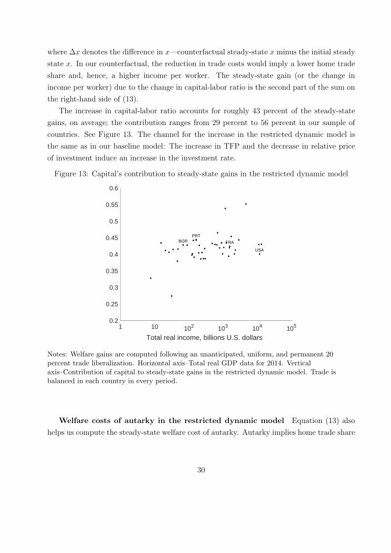
The increase in capital-labor ratio accounts for roughly 43 percent of the steady-state

gains, on average; the contribution ranges from 29 percent to 56 percent in our sample of

countries. See Figure 13. The channel for the increase in the restricted dynamic model is

the same as in our baseline model: The increase in TFP and the decrease in relative price

of investment induce an increase in the investment rate.

Figure 13: Capital’s contribution to steady-state gains in the restricted dynamic model

1 10 102 103 104 105

Total real income, billions U.S. dollars

0.2

0.25

0.3

0.35

0.4

0.45

0.5

0.55

0.6

...

BGR..

....

. ...

. .FRA..

..

..

.

.. ..

.

.

.

.

.

.. .PRT.

..

...

...

USA.

Notes: Welfare gains are computed following an unanticipated, uniform, and permanent 20percent trade liberalization. Horizontal axis–Total real GDP data for 2014. Verticalaxis–Contribution of capital to steady-state gains in the restricted dynamic model. Trade isbalanced in each country in every period.

Welfare costs of autarky in the restricted dynamic model Equation (13) also

helps us compute the steady-state welfare cost of autarky. Autarky implies home trade share

30

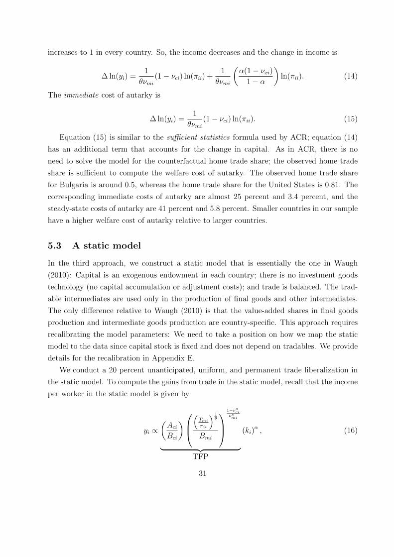
increases to 1 in every country. So, the income decreases and the change in income is

∆ ln(yi) =1

θνmi(1− νci) ln(πii) +

1

θνmi

(α(1− νxi)

1− α

)ln(πii). (14)

The immediate cost of autarky is

∆ ln(yi) =1

θνmi(1− νci) ln(πii). (15)

Equation (15) is similar to the sufficient statistics formula used by ACR; equation (14)

has an additional term that accounts for the change in capital. As in ACR, there is no

need to solve the model for the counterfactual home trade share; the observed home trade

share is sufficient to compute the welfare cost of autarky. The observed home trade share

for Bulgaria is around 0.5, whereas the home trade share for the United States is 0.81. The

corresponding immediate costs of autarky are almost 25 percent and 3.4 percent, and the

steady-state costs of autarky are 41 percent and 5.8 percent. Smaller countries in our sample

have a higher welfare cost of autarky relative to larger countries.

5.3 A static model

In the third approach, we construct a static model that is essentially the one in Waugh

(2010): Capital is an exogenous endowment in each country; there is no investment goods

technology (no capital accumulation or adjustment costs); and trade is balanced. The trad-

able intermediates are used only in the production of final goods and other intermediates.

The only difference relative to Waugh (2010) is that the value-added shares in final goods

production and intermediate goods production are country-specific. This approach requires

recalibrating the model parameters: We need to take a position on how we map the static

model to the data since capital stock is fixed and does not depend on tradables. We provide

details for the recalibration in Appendix E.

We conduct a 20 percent unanticipated, uniform, and permanent trade liberalization in

the static model. To compute the gains from trade in the static model, recall that the income

per worker in the static model is given by

yi ∝(AciBci

)(Tmiπii

) 1θ

Bmi

1−νsciνsmi

︸ ︷︷ ︸TFP

(ki)α , (16)

31

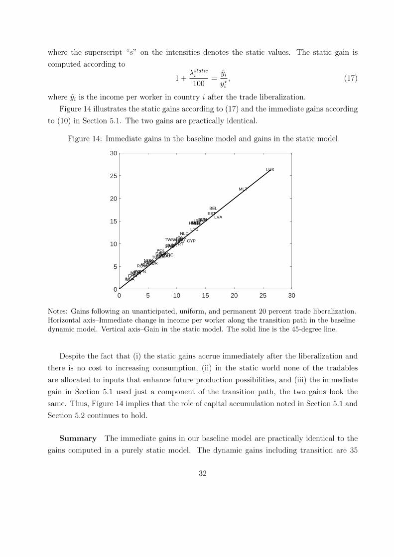
where the superscript “s” on the intensities denotes the static values. The static gain is

computed according to

1 +λstatici

100=yiy?i, (17)

where yi is the income per worker in country i after the trade liberalization.

Figure 14 illustrates the static gains according to (17) and the immediate gains according

to (10) in Section 5.1. The two gains are practically identical.

Figure 14: Immediate gains in the baseline model and gains in the static model

0 5 10 15 20 25 300

5

10

15

20

25

30

AUS

AUT

BEL

BGR

BRA

CAN

CHE

CHN

CYP

CZE

DEU

DNK

ESP

EST

FIN

FRA

GBR

GRC

HRV

HUN

IDN

IND

IRL

ITA

JPN

KOR

LTU

LUX

LVA

MEX

MLT

NLD

NOR

POL

PRT

ROU

ROWRUS

SVKSVN

SWE

TUR

TWN

USA

Notes: Gains following an unanticipated, uniform, and permanent 20 percent trade liberalization.Horizontal axis–Immediate change in income per worker along the transition path in the baselinedynamic model. Vertical axis–Gain in the static model. The solid line is the 45-degree line.

Despite the fact that (i) the static gains accrue immediately after the liberalization and

there is no cost to increasing consumption, (ii) in the static world none of the tradables

are allocated to inputs that enhance future production possibilities, and (iii) the immediate

gain in Section 5.1 used just a component of the transition path, the two gains look the

same. Thus, Figure 14 implies that the role of capital accumulation noted in Section 5.1 and

Section 5.2 continues to hold.

Summary The immediate gains in our baseline model are practically identical to the

gains computed in a purely static model. The dynamic gains including transition are 35

32

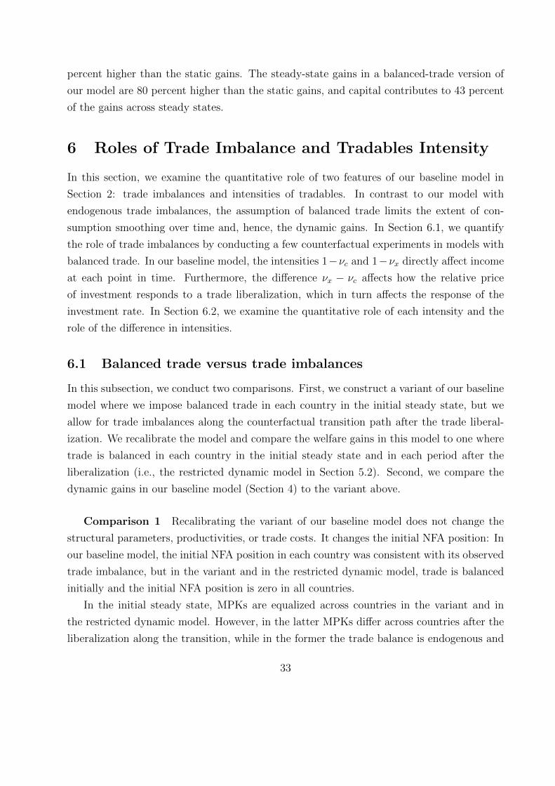
percent higher than the static gains. The steady-state gains in a balanced-trade version of

our model are 80 percent higher than the static gains, and capital contributes to 43 percent

of the gains across steady states.

6 Roles of Trade Imbalance and Tradables Intensity

In this section, we examine the quantitative role of two features of our baseline model in

Section 2: trade imbalances and intensities of tradables. In contrast to our model with

endogenous trade imbalances, the assumption of balanced trade limits the extent of con-

sumption smoothing over time and, hence, the dynamic gains. In Section 6.1, we quantify

the role of trade imbalances by conducting a few counterfactual experiments in models with

balanced trade. In our baseline model, the intensities 1−νc and 1−νx directly affect income

at each point in time. Furthermore, the difference νx − νc affects how the relative price

of investment responds to a trade liberalization, which in turn affects the response of the

investment rate. In Section 6.2, we examine the quantitative role of each intensity and the

role of the difference in intensities.

6.1 Balanced trade versus trade imbalances

In this subsection, we conduct two comparisons. First, we construct a variant of our baseline

model where we impose balanced trade in each country in the initial steady state, but we

allow for trade imbalances along the counterfactual transition path after the trade liberal-

ization. We recalibrate the model and compare the welfare gains in this model to one where

trade is balanced in each country in the initial steady state and in each period after the

liberalization (i.e., the restricted dynamic model in Section 5.2). Second, we compare the

dynamic gains in our baseline model (Section 4) to the variant above.

Comparison 1 Recalibrating the variant of our baseline model does not change the

structural parameters, productivities, or trade costs. It changes the initial NFA position: In

our baseline model, the initial NFA position in each country was consistent with its observed

trade imbalance, but in the variant and in the restricted dynamic model, trade is balanced

initially and the initial NFA position is zero in all countries.

In the initial steady state, MPKs are equalized across countries in the variant and in

the restricted dynamic model. However, in the latter MPKs differ across countries after the

liberalization along the transition, while in the former the trade balance is endogenous and

33

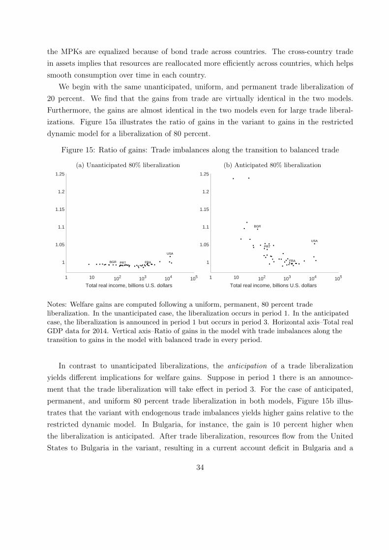
the MPKs are equalized because of bond trade across countries. The cross-country trade

in assets implies that resources are reallocated more efficiently across countries, which helps

smooth consumption over time in each country.

We begin with the same unanticipated, uniform, and permanent trade liberalization of

20 percent. We find that the gains from trade are virtually identical in the two models.

Furthermore, the gains are almost identical in the two models even for large trade liberal-

izations. Figure 15a illustrates the ratio of gains in the variant to gains in the restricted

dynamic model for a liberalization of 80 percent.

Figure 15: Ratio of gains: Trade imbalances along the transition to balanced trade

(a) Unanticipated 80% liberalization

1 10 102 103 104 105

Total real income, billions U.S. dollars

1

1.05

1.1

1.15

1.2

1.25

...BGR. ... .. . .. .. . FRA.... . . .. . ..... .. .. .PRT. . .... . ..USA.

(b) Anticipated 80% liberalization

1 10 102 103 104 105

Total real income, billions U.S. dollars

1

1.05

1.1

1.15

1.2

1.25

...

BGR.

... .

. .

.. .

.

.FRA..

.. .

. ... ..

.

.

.

.

.

.. .PRT.. ..

..

. ..

USA.

Notes: Welfare gains are computed following a uniform, permanent, 80 percent tradeliberalization. In the unanticipated case, the liberalization occurs in period 1. In the anticipatedcase, the liberalization is announced in period 1 but occurs in period 3. Horizontal axis–Total realGDP data for 2014. Vertical axis–Ratio of gains in the model with trade imbalances along thetransition to gains in the model with balanced trade in every period.

In contrast to unanticipated liberalizations, the anticipation of a trade liberalization

yields different implications for welfare gains. Suppose in period 1 there is an announce-

ment that the trade liberalization will take effect in period 3. For the case of anticipated,

permanent, and uniform 80 percent trade liberalization in both models, Figure 15b illus-

trates that the variant with endogenous trade imbalances yields higher gains relative to the

restricted dynamic model. In Bulgaria, for instance, the gain is 10 percent higher when

the liberalization is anticipated. After trade liberalization, resources flow from the United

States to Bulgaria in the variant, resulting in a current account deficit in Bulgaria and a

34

current account surplus in the United States. See Figure 16. These patterns imply that,

relative to the restricted dynamic model, Bulgaria front-loads consumption and the United

States back-loads consumption.8 In the case of an anticipated trade liberalization, these

effects will materialize before the liberalization happens, amplifying the effects of the trade

liberalization on consumption. The United States decreases consumption at the time of the

announcement, by running a large current account surplus. This feature is absent in the re-

stricted dynamic model and in models with unanticipated trade liberalization. By the time

the liberalization occurs in period 3, each country’s current account is at approximately the

same level as it would have been in an unanticipated trade liberalization.

The presence of trade imbalances introduces differences in rates of capital accumulation

across countries. Figures 16c and 16d show that, in the restricted dynamic model, invest-

ment falls at the time of the announcement because households postpone investment until

it becomes cheaper. In the world with trade imbalances, both the qualitative and quanti-

tative response of investment differs substantially across countries. Investment increases in

Bulgaria at the time of the announcement, while it decreases in the United States. This

is because Bulgaria runs a large current account deficit and uses the borrowed resources to

boost both consumption and investment, whereas the United States lends resources to the

rest of the world. Note that, in Bulgaria, the initial increase in investment is lower than

that in the case of an unanticipated trade liberalization, as households expect the relative

price to decrease. By period 3, investment reaches the same level as it would have been had

the trade liberalization been unanticipated. These findings imply that the reallocation of

resources from large to small countries during the periods prior to the trade liberalization

affect global efficiency and generate larger gains from trade relative to a model with balanced

trade in each period.

Comparison 2 We compare the welfare gains from an unanticipated, uniform, and

permanent trade liberalization of 20 percent in our baseline model to the gains in the variant

above. The difference between the two models is in the initial steady state: In our baseline

the current account balance is zero in each country and the NFA position is different across

countries, whereas in the variant the net exports and the NFA positions are both zero. Trade

imbalances are endogenous in the counterfactual in both models. Figure 17 illustrates the

ratio of gains in our baseline model to gains in the variant.

The gains in the variant do not depend on the initial NFA position since it is zero in

8This result is qualitatively consistent with the findings in Alessandria, Choi, and Lu (2017). They findthat anticipated reductions in trade costs result in borrowing for small open economies.

35

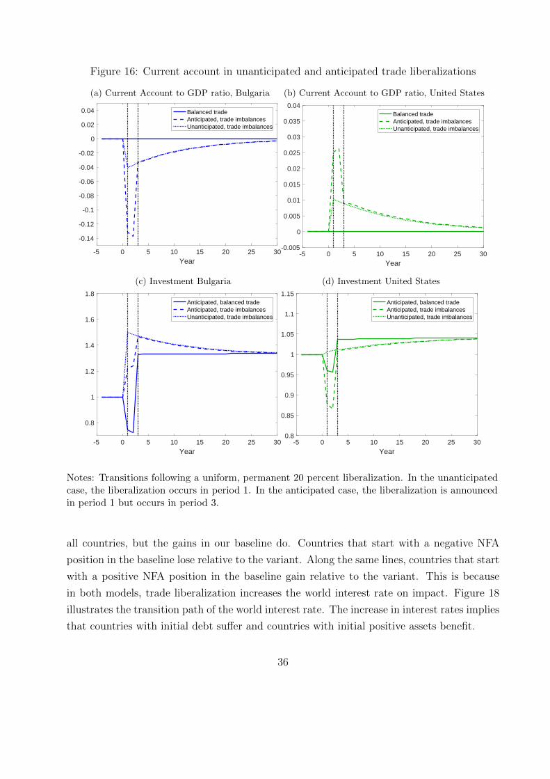
Figure 16: Current account in unanticipated and anticipated trade liberalizations

(a) Current Account to GDP ratio, Bulgaria

-5 0 5 10 15 20 25 30Year

-0.14

-0.12

-0.1

-0.08

-0.06

-0.04

-0.02

0

0.02

0.04 Balanced tradeAnticipated, trade imbalancesUnanticipated, trade imbalances

(b) Current Account to GDP ratio, United States

-5 0 5 10 15 20 25 30Year

-0.005

0

0.005

0.01

0.015

0.02

0.025

0.03

0.035

0.04Balanced tradeAnticipated, trade imbalancesUnanticipated, trade imbalances

(c) Investment Bulgaria

-5 0 5 10 15 20 25 30Year

0.8

1

1.2

1.4

1.6

1.8Anticipated, balanced tradeAnticipated, trade imbalancesUnanticipated, trade imbalances

(d) Investment United States

-5 0 5 10 15 20 25 30Year

0.8

0.85

0.9

0.95

1

1.05

1.1

1.15Anticipated, balanced tradeAnticipated, trade imbalancesUnanticipated, trade imbalances

Notes: Transitions following a uniform, permanent 20 percent liberalization. In the unanticipatedcase, the liberalization occurs in period 1. In the anticipated case, the liberalization is announcedin period 1 but occurs in period 3.

all countries, but the gains in our baseline do. Countries that start with a negative NFA

position in the baseline lose relative to the variant. Along the same lines, countries that start

with a positive NFA position in the baseline gain relative to the variant. This is because

in both models, trade liberalization increases the world interest rate on impact. Figure 18

illustrates the transition path of the world interest rate. The increase in interest rates implies

that countries with initial debt suffer and countries with initial positive assets benefit.

36

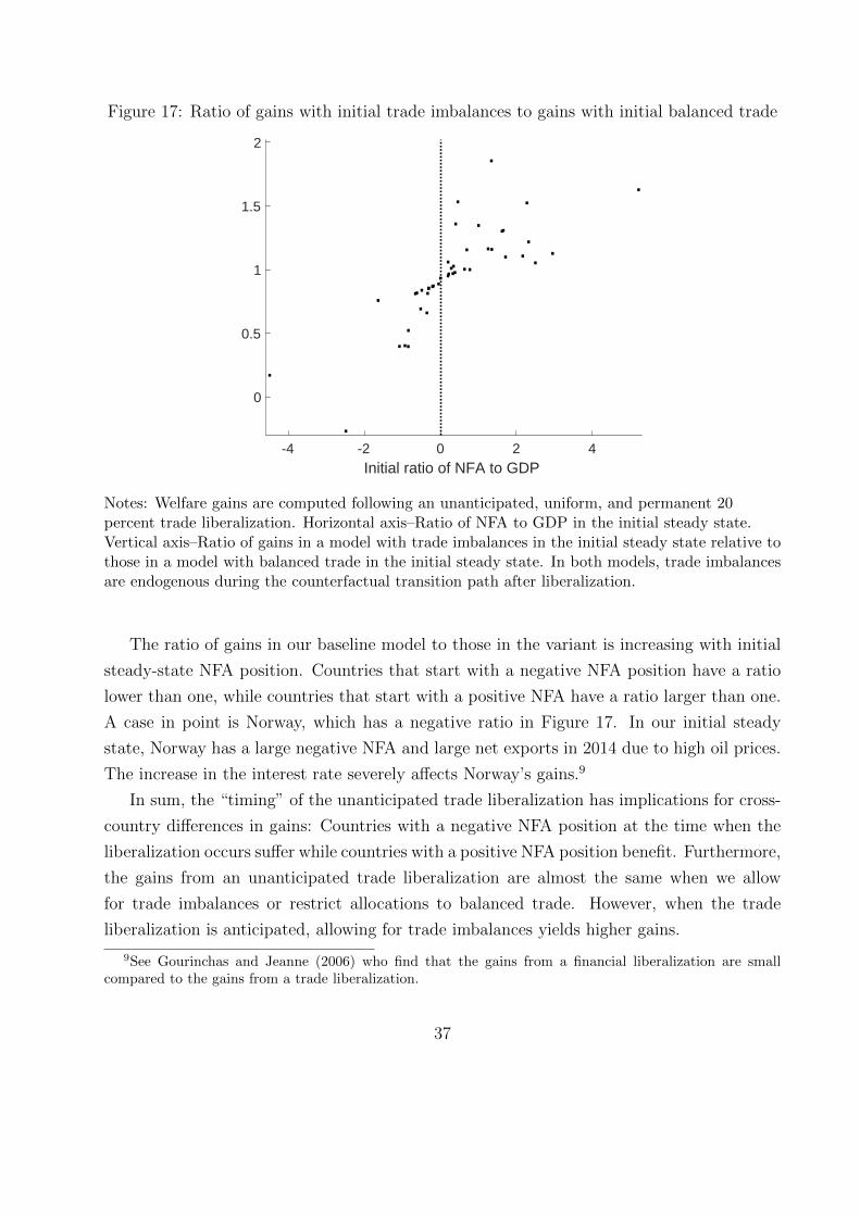
Figure 17: Ratio of gains with initial trade imbalances to gains with initial balanced trade

-4 -2 0 2 4Initial ratio of NFA to GDP

0

0.5

1

1.5

2

.

..

.

..

..

.

...

. ..

.. .

. .

.

.

.

.

.

.

. ... .

.

.

..

.

..

....

.

.

Notes: Welfare gains are computed following an unanticipated, uniform, and permanent 20percent trade liberalization. Horizontal axis–Ratio of NFA to GDP in the initial steady state.Vertical axis–Ratio of gains in a model with trade imbalances in the initial steady state relative tothose in a model with balanced trade in the initial steady state. In both models, trade imbalancesare endogenous during the counterfactual transition path after liberalization.

The ratio of gains in our baseline model to those in the variant is increasing with initial

steady-state NFA position. Countries that start with a negative NFA position have a ratio

lower than one, while countries that start with a positive NFA have a ratio larger than one.

A case in point is Norway, which has a negative ratio in Figure 17. In our initial steady

state, Norway has a large negative NFA and large net exports in 2014 due to high oil prices.

The increase in the interest rate severely affects Norway’s gains.9

In sum, the “timing” of the unanticipated trade liberalization has implications for cross-

country differences in gains: Countries with a negative NFA position at the time when the

liberalization occurs suffer while countries with a positive NFA position benefit. Furthermore,

the gains from an unanticipated trade liberalization are almost the same when we allow

for trade imbalances or restrict allocations to balanced trade. However, when the trade

liberalization is anticipated, allowing for trade imbalances yields higher gains.

9See Gourinchas and Jeanne (2006) who find that the gains from a financial liberalization are smallcompared to the gains from a trade liberalization.

37

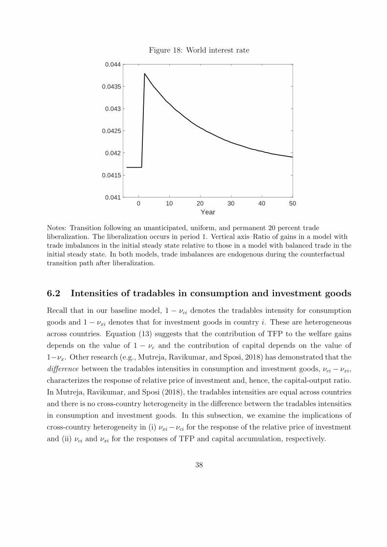
Figure 18: World interest rate

0 10 20 30 40 50Year

0.041

0.0415

0.042

0.0425

0.043

0.0435

0.044

Notes: Transition following an unanticipated, uniform, and permanent 20 percent tradeliberalization. The liberalization occurs in period 1. Vertical axis–Ratio of gains in a model withtrade imbalances in the initial steady state relative to those in a model with balanced trade in theinitial steady state. In both models, trade imbalances are endogenous during the counterfactualtransition path after liberalization.

6.2 Intensities of tradables in consumption and investment goods

Recall that in our baseline model, 1 − νci denotes the tradables intensity for consumption

goods and 1− νxi denotes that for investment goods in country i. These are heterogeneous

across countries. Equation (13) suggests that the contribution of TFP to the welfare gains

depends on the value of 1 − νc and the contribution of capital depends on the value of

1−νx. Other research (e.g., Mutreja, Ravikumar, and Sposi, 2018) has demonstrated that the

difference between the tradables intensities in consumption and investment goods, νci − νxi,characterizes the response of relative price of investment and, hence, the capital-output ratio.

In Mutreja, Ravikumar, and Sposi (2018), the tradables intensities are equal across countries

and there is no cross-country heterogeneity in the difference between the tradables intensities

in consumption and investment goods. In this subsection, we examine the implications of

cross-country heterogeneity in (i) νxi−νci for the response of the relative price of investment

and (ii) νci and νxi for the responses of TFP and capital accumulation, respectively.

38

Effect on the relative price of investment In our baseline calibration in Section

3, investment goods are more tradables-intensive than consumption goods (νxi < νci), which

implies that the relative price of investment falls after a trade liberalization. The magnitude

of the decline in the relative price of investment differs across countries and affects the

investment rate and the capital-output ratio. Equation (18) shows that the change in the

relative price of investment is driven by: (i) the change in the home trade share and (ii)

magnitude of νxi − νci:

PxitPcit∝(Bxi

Bci

)(AciAxi

)(Tmiπii

) 1θ

Bmi

νxi−νciνmi

. (18)

.

In order to isolate the roles of (i) and (ii), we first show that the response of the home

trade share is virtually independent of the values of νxi and νci. To illustrate this, suppose

that all countries have the same νx and the same νc. Specifically, we find the country with

the maximum difference between νx and νc, which in our sample is India. Denote India’s

intensities by νx and νc. We set νxi = νx and νci = νc for all i; this imposes maximal difference

between νx and νc but eliminates the heterogeneity in the intensities. We implement the

counterfactual 20 percent trade liberalization. Figure 19 illustrates transition paths for the

home trade share and the relative price of investment in Bulgaria and the United States.

We find that the path for home trade share after the liberalization is almost identical to

the path in our baseline model with heterogeneous intensities. Figures 19a and 19b illustrate

that the cross-country heterogeneity in either of the tradables intensity does not affect the

response of home trade shares. However, Figures 19c and 19d illustrate that the relative price

falls by more than in the baseline model. This is because of the greater difference between the

tradables intensities in consumption goods and investment goods: Larger νci − νxi implies

that trade liberalization reduces the relative price of investment more; see equation (18).

Thus, the cross-country heterogeneity in the difference in tradables intensities affects the

response of the relative price of investment. Below we demonstrate a less well known result:

Cross-country heterogeneity in each tradables intensity affects the responses of TFP and

capital-labor ratio and, hence, their contributions to welfare gains from trade.

Effects on TFP and capital accumulation Next, we explore how the magnitudes

of νxi and νci individually affect TFP and capital accumulation after a trade liberalization.

Since changes in these parameters have an effect on the relative price of investment, we

39

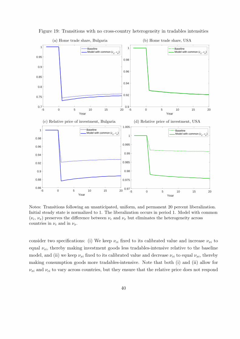
Figure 19: Transitions with no cross-country heterogeneity in tradables intensities

(a) Home trade share, Bulgaria

-5 0 5 10 15 20Year

0.7

0.75

0.8

0.85

0.9

0.95

1BaselineModel with common (

c,

x)

(b) Home trade share, USA

-5 0 5 10 15 20Year

0.9

0.92

0.94

0.96

0.98

1 BaselineModel with common (

c,

x)

(c) Relative price of investment, Bulgaria

-5 0 5 10 15 20Year

0.86

0.88

0.9

0.92

0.94

0.96

0.98

1 BaselineModel with common (

c,

x)

(d) Relative price of investment, USA

-5 0 5 10 15 20Year

0.97

0.975

0.98

0.985

0.99

0.995

1

1.005BaselineModel with common (

c,

x)

Notes: Transitions following an unanticipated, uniform, and permanent 20 percent liberalization.Initial steady state is normalized to 1. The liberalization occurs in period 1. Model with common(νc, νx) preserves the difference between νc and νx but eliminates the heterogeneity acrosscountries in νc and in νx.

consider two specifications: (i) We keep νci fixed to its calibrated value and increase νxi to

equal νci, thereby making investment goods less tradables-intensive relative to the baseline

model, and (ii) we keep νxi fixed to its calibrated value and decrease νci to equal νxi, thereby

making consumption goods more tradables-intensive. Note that both (i) and (ii) allow for

νxi and νci to vary across countries, but they ensure that the relative price does not respond

40

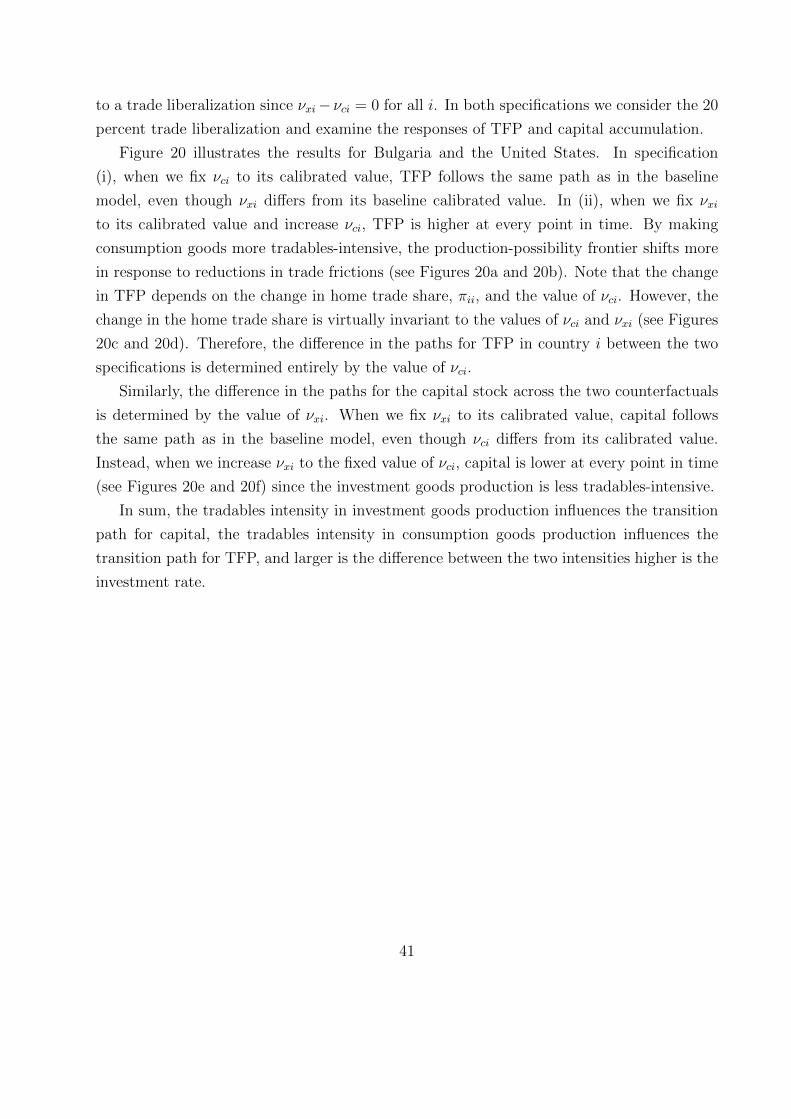
to a trade liberalization since νxi− νci = 0 for all i. In both specifications we consider the 20

percent trade liberalization and examine the responses of TFP and capital accumulation.

Figure 20 illustrates the results for Bulgaria and the United States. In specification

(i), when we fix νci to its calibrated value, TFP follows the same path as in the baseline

model, even though νxi differs from its baseline calibrated value. In (ii), when we fix νxi

to its calibrated value and increase νci, TFP is higher at every point in time. By making

consumption goods more tradables-intensive, the production-possibility frontier shifts more

in response to reductions in trade frictions (see Figures 20a and 20b). Note that the change

in TFP depends on the change in home trade share, πii, and the value of νci. However, the

change in the home trade share is virtually invariant to the values of νci and νxi (see Figures

20c and 20d). Therefore, the difference in the paths for TFP in country i between the two

specifications is determined entirely by the value of νci.

Similarly, the difference in the paths for the capital stock across the two counterfactuals

is determined by the value of νxi. When we fix νxi to its calibrated value, capital follows

the same path as in the baseline model, even though νci differs from its calibrated value.

Instead, when we increase νxi to the fixed value of νci, capital is lower at every point in time

(see Figures 20e and 20f) since the investment goods production is less tradables-intensive.

In sum, the tradables intensity in investment goods production influences the transition

path for capital, the tradables intensity in consumption goods production influences the

transition path for TFP, and larger is the difference between the two intensities higher is the

investment rate.

41

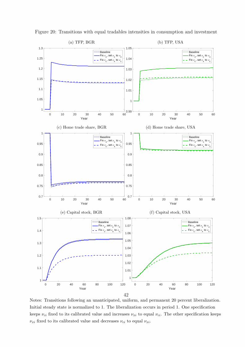
Figure 20: Transitions with equal tradables intensities in consumption and investment

(a) TFP, BGR

0 10 20 30 40 50 60Year

1

1.05

1.1

1.15

1.2

1.25

1.3BaselineFix

x, set

c to

x

Fix c, set

x to

c

(b) TFP, USA

0 10 20 30 40 50 60Year

0.99

1

1.01

1.02

1.03

1.04

1.05BaselineFix

x, set

c to

x

Fix c, set

x to

c

(c) Home trade share, BGR

0 10 20 30 40 50 60Year

0.7

0.75

0.8

0.85

0.9

0.95

1BaselineFix

x, set

c to

x

Fix c, set

x to

c

(d) Home trade share, USA

0 10 20 30 40 50 60Year

0.7

0.75

0.8

0.85

0.9

0.95

1BaselineFix

x, set

c to

x

Fix c, set

x to

c

(e) Capital stock, BGR

0 20 40 60 80 100 120Year

1

1.1

1.2

1.3

1.4

1.5BaselineFix

x, set

c to

x

Fix c, set

x to

c

(f) Capital stock, USA

0 20 40 60 80 100 120Year

1

1.01

1.02

1.03

1.04

1.05

1.06

1.07

1.08BaselineFix

x, set

c to

x

Fix c, set

x to

c

Notes: Transitions following an unanticipated, uniform, and permanent 20 percent liberalization.

Initial steady state is normalized to 1. The liberalization occurs in period 1. One specification

keeps νci fixed to its calibrated value and increases νxi to equal νci. The other specification keeps

νxi fixed to its calibrated value and decreases νci to equal νxi.

42

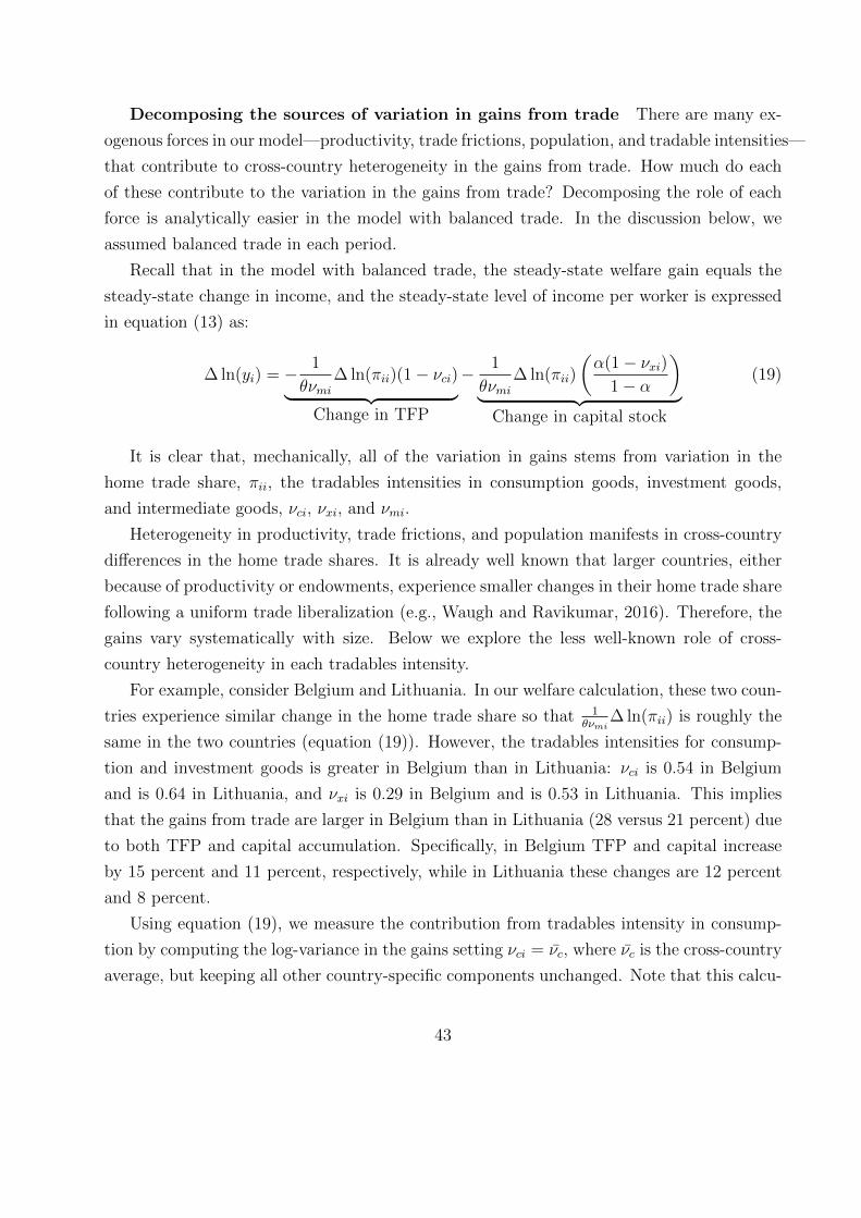
Decomposing the sources of variation in gains from trade There are many ex-

ogenous forces in our model—productivity, trade frictions, population, and tradable intensities—

that contribute to cross-country heterogeneity in the gains from trade. How much do each

of these contribute to the variation in the gains from trade? Decomposing the role of each

force is analytically easier in the model with balanced trade. In the discussion below, we

assumed balanced trade in each period.

Recall that in the model with balanced trade, the steady-state welfare gain equals the

steady-state change in income, and the steady-state level of income per worker is expressed

in equation (13) as:

∆ ln(yi) = − 1

θνmi∆ ln(πii)(1− νci)︸ ︷︷ ︸

Change in TFP

− 1

θνmi∆ ln(πii)

(α(1− νxi)

1− α

)︸ ︷︷ ︸

Change in capital stock

(19)

It is clear that, mechanically, all of the variation in gains stems from variation in the

home trade share, πii, the tradables intensities in consumption goods, investment goods,

and intermediate goods, νci, νxi, and νmi.

Heterogeneity in productivity, trade frictions, and population manifests in cross-country

differences in the home trade shares. It is already well known that larger countries, either

because of productivity or endowments, experience smaller changes in their home trade share

following a uniform trade liberalization (e.g., Waugh and Ravikumar, 2016). Therefore, the

gains vary systematically with size. Below we explore the less well-known role of cross-

country heterogeneity in each tradables intensity.

For example, consider Belgium and Lithuania. In our welfare calculation, these two coun-

tries experience similar change in the home trade share so that 1θνmi

∆ ln(πii) is roughly the

same in the two countries (equation (19)). However, the tradables intensities for consump-

tion and investment goods is greater in Belgium than in Lithuania: νci is 0.54 in Belgium

and is 0.64 in Lithuania, and νxi is 0.29 in Belgium and is 0.53 in Lithuania. This implies

that the gains from trade are larger in Belgium than in Lithuania (28 versus 21 percent) due

to both TFP and capital accumulation. Specifically, in Belgium TFP and capital increase

by 15 percent and 11 percent, respectively, while in Lithuania these changes are 12 percent

and 8 percent.

Using equation (19), we measure the contribution from tradables intensity in consump-

tion by computing the log-variance in the gains setting νci = νc, where νc is the cross-country

average, but keeping all other country-specific components unchanged. Note that this calcu-

43

lation assumes that the home trade share is approximately invariant to changes in νci, which

we have already shown to be the case in Figure 19 and Figure 20. We find that the log

variance in gains declines by 26 percent. For example, Luxembourg experiences the largest

decline in gains after removing the heterogeneity in νci. The value for νci in Luxembourg in-

creases from 0.27 to 0.56 and their welfare gains decrease from 30 percent to 22 percent. On

the other hand, Mexico experiences the largest increase in gains. The value for νci in Mexico

decreases from 0.75 to 0.56 and their welfare gains increase from 6 percent to 8 percent.

Similarly, we measure the contribution from tradables intensity in investment by com-

puting the log-variance in the gains setting νxi = νx, but keeping all other country-specific

components unchanged. As in the previous case, the home trade share is approximately

invariant to changes in νxi. We find that the log variance in gains declines by 3 percent. For

example, China experiences the largest decline in gains after removing the heterogeneity in

νxi. The value for νxi in China increases from 0.20 to 0.33 and their welfare gains decrease

from 4.4 percent to 4.1 percent. On the other hand, Lithuania experiences the largest in-

crease in gains. The value for νxi in Lithuania decreases from 0.53 to 0.56 and their welfare

gains increase from 19 percent to 22 percent.

These two exercises imply that a substantial portion of the log variance in gains is ac-

counted for the cross-country variations in νm and in the reduction in home trade shares.

7 Conclusion

We build a multicountry trade model with capital accumulation to study dynamic welfare

gains. In our model, tradable intermediates are used in the production of final consumption

goods and investment goods with different intensities. Cross-country asset trades generate

endogenous trade imbalances and help smooth consumption over time.

Trade liberalization increases total factor productivity, which increases the rate of return

to investment and, hence, the capital stock. As capital accumulates, output and consumption

increase and the welfare gains accrue gradually over time. Trade liberalization also reduces

the relative price of tradables, altering the rate of transformation between consumption and

investment. This boosts the share of output allocated to investment and allows countries

attain, yet, even higher capital-output ratios.

For an unanticipated, uniform, and permanent reduction in trade costs, we find that the

gains are negatively correlated with size; financial resources flow from larger countries to

smaller countries; countries with larger short-run trade deficits accumulate capital faster;

44

smaller countries front-load their consumption, while larger countries do the opposite; the

gains are nonlinear in the reduction in trade costs; and capital accumulation delivers sub-

stantial gains relative to a model where capital is fixed. And, the gains are higher when the

trade liberalization is anticipated.

The NFA position before the liberalization and the tradables intensities in investment

goods production and consumption goods production are quantitatively important for the

gains. The liberalization increases the world interest rate on impact, which implies that

countries with initial debt suffer and countries with initial positive assets benefit. The

transition path for capital depends almost entirely on the tradables intensity in investment

goods production and the transition of path of TFP depends exclusively on the tradables

intensity in consumption goods production.

Our computational algorithm efficiently solves for the exact transitional dynamics for a

system of second-order, nonlinear difference equations. Our method iterates on prices using

excess demand functions and does not involve costly gradient calculations, and it delivers

the transition paths for all countries in less than two hours. Thus, our method is useful

for solving multicountry trade models with large state spaces. Our solution method can

also be used to analyze other changes in trade costs, such as multilateral trade agreements

with gradual reductions in trade barriers (e.g., European Union and NAFTA), anticipated

changes in trade costs (e.g., Brexit), and other models with multiple sectors and IO linkages.

With diminishing returns to capital accumulation, we have clearly abstracted from the

effect of trade costs on long-run growth. Our model can be extended to incorporate long-run

growth and study the gains from trade resulting from changes in the rate of long-run growth.

One avenue is to assume constant returns to capital accumulation (the so-called “Ak” model)

and bound the marginal product of capital to be sufficiently far away from zero. In such

a model, the trade cost affects the return to capital and, hence, the investment rate and

the rate of long-run growth (see Lee (1993), for instance, for a small open Ak economy).

Another avenue is to introduce an R&D sector into our model as in the two-country model

of Grossman and Helpman (1990). In such a model, investment in R&D expands the variety

of intermediate goods which increases TFP in the final goods sector. The investment also

helps accumulate knowledge that is not subject to diminishing returns. Trade cost then

affects the rates of knowledge accumulation and TFP growth. Changes in trade cost in both

models affect the rate of long run growth and, hence, the gains from trade.

45

References

Adao, Rodrigo, Arnaud Costinot, and Dave Donaldson. 2017. “Nonparametric Counter-

factual Predictions in Neoclassical Models of International Trade.” American Economic

Review 107 (3):633–689.

Alessandria, George, Horag Choi, and Dan Lu. 2017. “Trade Integration and the Trade

Balance in China.” IMF Economic Review 65 (3):633–674.

Alessandria, George, Horag Choi, and Kim Ruhl. 2014. “Trade adjustment dynamics and

the welfare gains from trade.” Working paper, National Bureau of Economic Research.

Alvarez, Fernando and Robert E. Lucas. 2007. “General Equilibrium Analysis of the Eaton-

Kortum Model of International Trade.” Journal of Monetary Economics 54 (6):1726–1768.

———. 2017. “Capital Accumulation and International Trade.” Journal of Monetary Eco-

nomics 91:1–18.

Anderson, James, Mario Larch, and Yoto Yotov. 2015. “Growth and Trade with Frictions: A

Structural Estimation Framework.” Working Paper 21377, National Bureau of Economic

Research.

Arkolakis, Costas, Arnaud Costinot, and Andres Rodrıguez-Clare. 2012. “New Trade Models,

Same Old Gains?” American Economic Review 102 (1):94–130.

Baldwin, Richard E. 1992. “Measurable dynamic gains from trade.” Journal of Political

Economy 100 (1):162–174.

Bernard, Andrew B., Jonathan Eaton, J. Bradford Jensen, and Samuel Kortum.

2003. “Plants and Productivity in International Trade.” American Economic Review

93 (4):1268–1290.

Brooks, Wyatt J. and Pau S. Pujolas. 2016. “Capital Accumulation and the Welfare Gains

from Trade.” Working Paper Series 2016-03, McMaster University.

Caliendo, Lorenzo, Maximiliano Dvorkin, and Fernando Parro. 2017. “Trade and Labor

Market Dynamics: General Equilibrium Analysis of the China Trade Shock.” NBER

Working Paper 77999.

46

Caliendo, Lorenzo and Fernando Parro. 2015. “Estimates of the Trade and Welfare Effects

of NAFTA.” Tech. rep.

Connolly, Michelle and Kei-Mu Yi. 2015. “How Much of South Korea’s Growth Miracle

Can Be Explained by Trade Policy?” American Economic Journal: Macroeconomics

7 (4):188–221.

Eaton, Jonathan and Samuel Kortum. 2002. “Technology, Geography, and Trade.” Econo-

metrica 70 (5):1741–1779.

Eaton, Jonathan, Samuel Kortum, Brent Neiman, and John Romalis. 2016. “Trade and the

Global Recession.” American Economic Review 106 (11):3401–3438.

Feenstra, Robert C., Robert Inklaar, and Marcel Timmer. 2015. “The Next Generation of

the Penn World Table.” American Economic Review 105 (10):3150–82.

Gollin, Douglas. 2002. “Getting Income Shares Right.” Journal of Political Economy

110 (2):458–474.

Gourinchas, Pierre-Olivier and Olivier Jeanne. 2006. “The elusive gains from international

financial integration.” The Review of Economic Studies 73 (3):715–741.

Grossman, Gene M and Elhanan Helpman. 1990. “Trade, innovation, and growth.” The

American economic review 80 (2):86–91.

Kehoe, Timothy J., Kim J. Ruhl, and Joseph P. Steinberg. 2016. “Global Imbalances and

Structural Change in the United States.” NBER Working Papers 19339, National Bureau

of Economic Research.

Lee, Jong-Wha. 1993. “International trade, distortions, and long-run economic growth.”

Staff papers 40 (2):299–328.

Lucas, Robert E. 1987. Models of Business Cycles, vol. 26. Basil Blackwell Oxford.

Mutreja, Piyusha, B. Ravikumar, and Michael Sposi. 2018. “Capital Goods Trade, Relative

Prices, and Economic Development.” Review of Economic Dynamics 27:101–122.

Reyes-Heroles, Ricardo. 2016. “The Role of Trade Costs in the Surge of Trade Imbalances.”

Mimeo, Princeton University.

47

Simonovska, Ina and Michael E. Waugh. 2014. “The Elasticity of Trade: Estimates and

Evidence.” Journal of International Economics 92 (1):34–50.

Sposi, Michael. 2012. “Evolving Comparative Advantage, Structural Change, and the Com-

position of Trade.” Mimeo, University of Iowa.

Timmer, Marcel P., Erik Dietzenbacher, Bart Los, and Gaaitzen J. de Vries. 2015. “An

Illustrated Guide to the World Input-Output Database: The Case of Global Automotive

Production.” Review of International Economics 23 (3):575–605.

Timmer, Marcel P., Bart Los, Robert Stehrer, and Gaaitzen J. de Vries. 2016. “An Anatomy

of the Global Trade Slowdown based on the WIOD 2016 Release.” GGDC research mem-

orandum 162, University of Groningen.

Wacziarg, Romain and Karen Horn Welch. 2008. “International Trade and Income Differ-

ences.” World Bank Economic Review 22 (2):187–231.

Waugh, Michael E. 2010. “International Trade and Income Differences.” American Economic

Review 22 (5):2093–2124.

Waugh, Michael E. and B. Ravikumar. 2016. “Measuring openness to trade.” Journal of

Economic Dynamics and Control 72:29–41.

Zylkin, Thomas. 2016. “Feeding China’s Rise: The Growth Effects of Trading with China,

1993-2011.” GPN working paper series, National University of Singapore.

48

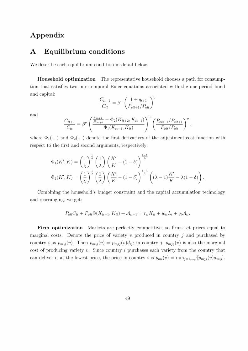
Appendix

A Equilibrium conditions

We describe each equilibrium condition in detail below.

Household optimization The representative household chooses a path for consump-

tion that satisfies two intertemporal Euler equations associated with the one-period bond

and capital:Cit+1

Cit= βσ

(1 + qt+1

Pcit+1/Pcit

)σand

Cit+1

Cit= βσ

( rit+1

Pixt+1− Φ2(Kit+2, Kit+1)

Φ1(Kit+1, Kit)

)σ (Pxit+1/Pcit+1

Pxit/Pcit

)σ,

where Φ1(·, ·) and Φ2(·, ·) denote the first derivatives of the adjustment-cost function with

respect to the first and second arguments, respectively:

Φ1(K ′, K) =

(1

χ

) 1λ(

1

λ

)(K ′

K− (1− δ)

) 1−λλ

Φ2(K ′, K) =

(1

χ

) 1λ(

1

λ

)(K ′

K− (1− δ)

) 1−λλ(

(λ− 1)K ′

K− λ(1− δ)

).

Combining the household’s budget constraint and the capital accumulation technology

and rearranging, we get:

PcitCit + PxitΦ(Kit+1, Kit) +Ait+1 = ritKit + witLi + qtAit.

Firm optimization Markets are perfectly competitive, so firms set prices equal to

marginal costs. Denote the price of variety v produced in country j and purchased by

country i as pmij(v). Then pmij(v) = pmjj(v)dij; in country j, pmjj(v) is also the marginal

cost of producing variety v. Since country i purchases each variety from the country that

can deliver it at the lowest price, the price in country i is pmi(v) = minj=1,...,I [pmjj(v)dmij].

49

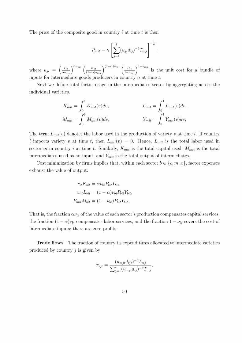
The price of the composite good in country i at time t is then

Pmit = γ

[I∑j=1

(ujtdij)−θTmj

]− 1θ

,

where ujt =(

rjtανmj

)ανmj ( wjt(1−α)νmj

)(1−α)νmj ( Pjt1−νmj

)1−νmjis the unit cost for a bundle of

inputs for intermediate goods producers in country n at time t.

Next we define total factor usage in the intermediates sector by aggregating across the

individual varieties.

Kmit =

∫ 1

0

Kmit(v)dv, Lmit =

∫ 1

0

Lmit(v)dv,

Mmit =

∫ 1

0

Mmit(v)dv, Ymit =

∫ 1

0

Ymit(v)dv.

The term Lmit(v) denotes the labor used in the production of variety v at time t. If country

i imports variety v at time t, then Lmit(v) = 0. Hence, Lmit is the total labor used in

sector m in country i at time t. Similarly, Kmit is the total capital used, Mmit is the total

intermediates used as an input, and Ymit is the total output of intermediates.

Cost minimization by firms implies that, within each sector b ∈ {c,m, x}, factor expenses

exhaust the value of output:

ritKbit = ανbiPbitYbit,

witLbit = (1− α)νbiPbitYbit,

PmitMbit = (1− νbi)PbitYbit.

That is, the fraction ανbi of the value of each sector’s production compensates capital services,

the fraction (1−α)νbi compensates labor services, and the fraction 1− νbi covers the cost of

intermediate inputs; there are zero profits.

Trade flows The fraction of country i’s expenditures allocated to intermediate varieties

produced by country j is given by

πijt =(umjtdijt)

−θTmj∑Ij=1(umjtdij)−θTmj

,

50

where umjt is the unit cost of intermediate varieties in country j.

Market clearing The domestic factor market-clearing conditions are:∑b∈{c,m,x}

Kbit = Kit,∑

b∈{c,m,x}

Lbit = Li,∑

b∈{c,m,x}

Mbit = Mit.

The first two conditions impose that the capital and labor markets clear in country i at each

time t. The third condition requires that the use of the composite good equals its supply.

Its use consists of demand by firms in each sector. Its supply consists of both domestically

and foreign-produced varieties.

The next set of conditions require that goods markets clear.

Cit = Ycit, Xit = Yxit,I∑j=1

Pmjt (Mcjt +Mmjt +Mxjt)πjit = PmitYmit.

The first condition states that the quantity of (nontradable) consumption demanded by the

representative household in country i must equal the quantity produced by country i. The

second condition says the same for the investment good. The third condition imposes that

the value of intermediates produced by country i has to be absorbed globally. Recall that

PmjtMbjt is the value of intermediate inputs that country i uses in production in sector b.

The term πjit is the fraction of country j’s intermediate good expenditures sourced from

country i. Therefore, PmjtMbjtπjit denotes the value of trade flows from country i to j.

Finally, we impose an aggregate resource constraint in each country: Net exports equal

zero. Equivalently, gross output equals gross absorption:

Bit = PmitYmit − PmitMit + qtAit.

Given an initial NFA position and capital stock, the equilibrium transition path consists

of the following objects: {~wt}Tt=1, {~rt}Tt=1, {qt}Tt=1, {~Pct}Tt=1, {~Pmt}Tt=1, {~Pxt}Tt=1, {~Ct}Tt=1,

{ ~Xt}Tt=1, { ~Kt}T+1t=1 , { ~Bt}Tt=1,{ ~At}T+1

t=1 , {~Yct}Tt=1, {~Ymt}Tt=1, {~Yxt}Tt=1, { ~Kct}Tt=1, { ~Kmt}Tt=1, { ~Kxt}Tt=1,

{~Lct}Tt=1, {~Lmt}Tt=1, {~Lxt}Tt=1, { ~Mct}Tt=1, { ~Mmt}Tt=1, { ~Mxt}Tt=1, {~~πt}Tt=1. (The double-arrow no-

tation on ~~πt is used to indicate that this is an I × I matrix in each period t.) Table A.1

provides a list of equilibrium conditions that these objects must satisfy.

In this environment, the world interest rate is strictly nominal. That is, the prices map

into current units, as opposed to constant units. In other words, the model can be rewritten

51

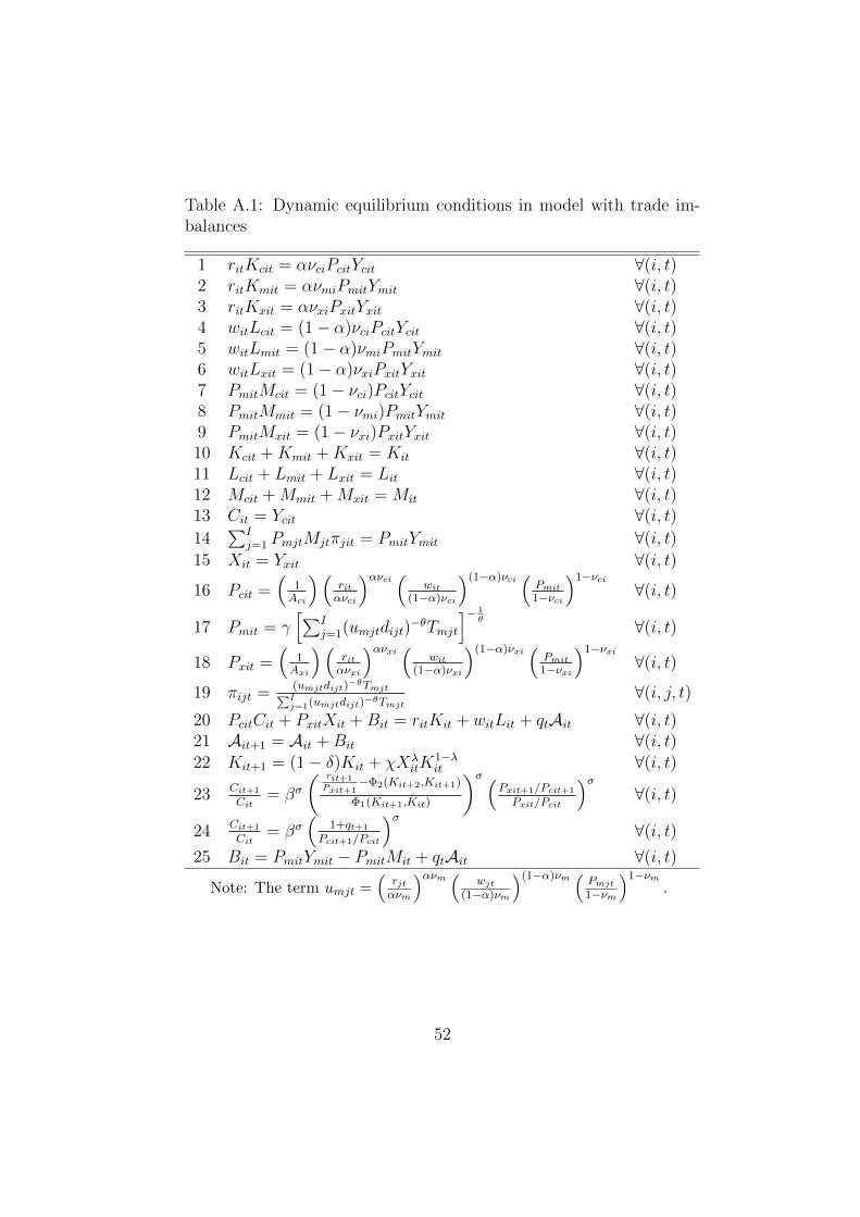
Table A.1: Dynamic equilibrium conditions in model with trade im-balances

1 ritKcit = ανciPcitYcit ∀(i, t)2 ritKmit = ανmiPmitYmit ∀(i, t)3 ritKxit = ανxiPxitYxit ∀(i, t)4 witLcit = (1− α)νciPcitYcit ∀(i, t)5 witLmit = (1− α)νmiPmitYmit ∀(i, t)6 witLxit = (1− α)νxiPxitYxit ∀(i, t)7 PmitMcit = (1− νci)PcitYcit ∀(i, t)8 PmitMmit = (1− νmi)PmitYmit ∀(i, t)9 PmitMxit = (1− νxi)PxitYxit ∀(i, t)10 Kcit +Kmit +Kxit = Kit ∀(i, t)11 Lcit + Lmit + Lxit = Lit ∀(i, t)12 Mcit +Mmit +Mxit = Mit ∀(i, t)13 Cit = Ycit ∀(i, t)14

∑Ij=1 PmjtMjtπjit = PmitYmit ∀(i, t)

15 Xit = Yxit ∀(i, t)

16 Pcit =(

1Aci

)(ritανci

)ανci (wit

(1−α)νci

)(1−α)νci (Pmit1−νci

)1−νci∀(i, t)

17 Pmit = γ[∑I

j=1(umjtdijt)−θTmjt

]− 1θ ∀(i, t)

18 Pxit =(

1Axi

)(ritανxi

)ανxi (wit

(1−α)νxi

)(1−α)νxi (Pmit1−νxi

)1−νxi∀(i, t)

19 πijt =(umjtdijt)

−θTmjt∑Ij=1(umjtdijt)−θTmjt

∀(i, j, t)20 PcitCit + PxitXit +Bit = ritKit + witLit + qtAit ∀(i, t)21 Ait+1 = Ait +Bit ∀(i, t)22 Kit+1 = (1− δ)Kit + χXλ

itK1−λit ∀(i, t)

23 Cit+1

Cit= βσ

( rit+1Pxit+1

−Φ2(Kit+2,Kit+1)

Φ1(Kit+1,Kit)

)σ (Pxit+1/Pcit+1

Pxit/Pcit

)σ∀(i, t)

24 Cit+1

Cit= βσ

(1+qt+1

Pcit+1/Pcit

)σ∀(i, t)

25 Bit = PmitYmit − PmitMit + qtAit ∀(i, t)

Note: The term umjt =(rjtανm

)ανm ( wjt(1−α)νm

)(1−α)νm ( Pmjt1−νm

)1−νm.

52

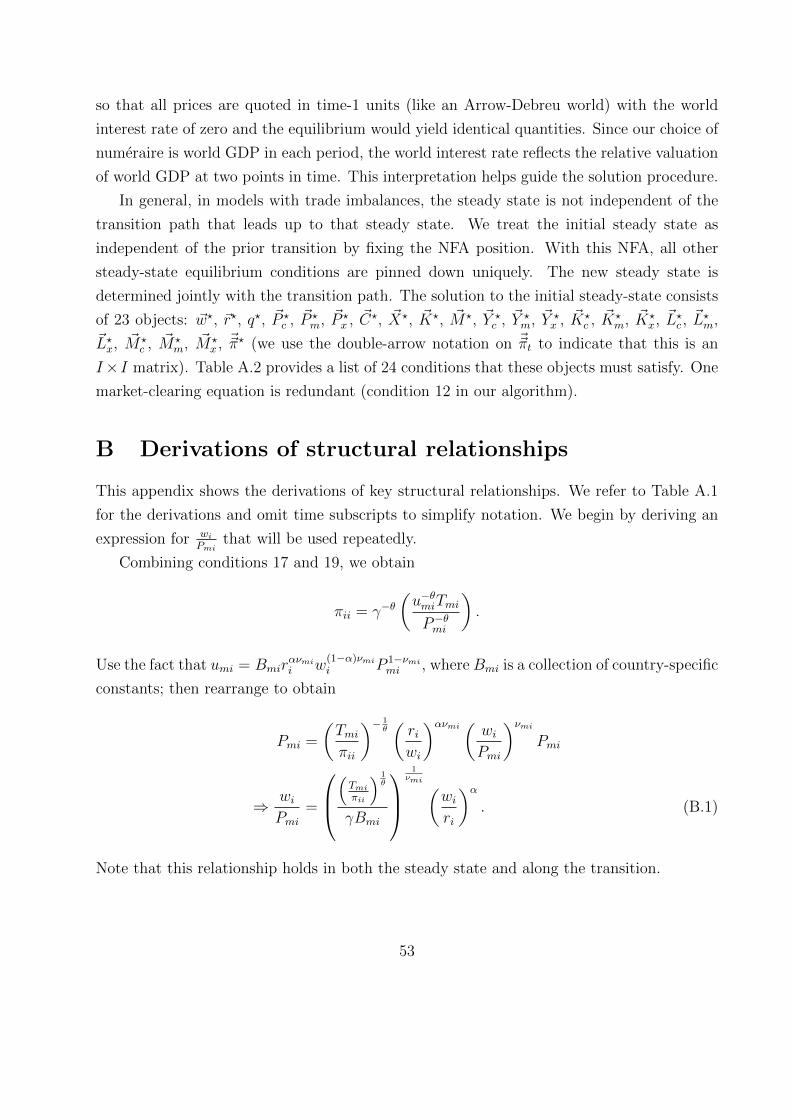
so that all prices are quoted in time-1 units (like an Arrow-Debreu world) with the world

interest rate of zero and the equilibrium would yield identical quantities. Since our choice of

numeraire is world GDP in each period, the world interest rate reflects the relative valuation

of world GDP at two points in time. This interpretation helps guide the solution procedure.

In general, in models with trade imbalances, the steady state is not independent of the

transition path that leads up to that steady state. We treat the initial steady state as

independent of the prior transition by fixing the NFA position. With this NFA, all other

steady-state equilibrium conditions are pinned down uniquely. The new steady state is

determined jointly with the transition path. The solution to the initial steady-state consists

of 23 objects: ~w?, ~r?, q?, ~P ?c , ~P ?

m, ~P ?x , ~C?, ~X?, ~K?, ~M?, ~Y ?

c , ~Y ?m, ~Y ?

x , ~K?c , ~K?

m, ~K?x, ~L?c , ~L

?m,

~L?x, ~M?c , ~M?

m, ~M?x , ~~π? (we use the double-arrow notation on ~~πt to indicate that this is an

I×I matrix). Table A.2 provides a list of 24 conditions that these objects must satisfy. One

market-clearing equation is redundant (condition 12 in our algorithm).

B Derivations of structural relationships

This appendix shows the derivations of key structural relationships. We refer to Table A.1

for the derivations and omit time subscripts to simplify notation. We begin by deriving an

expression for wiPmi

that will be used repeatedly.

Combining conditions 17 and 19, we obtain

πii = γ−θ(u−θmiTmi

P−θmi

).

Use the fact that umi = Bmirανmii w

(1−α)νmii P 1−νmi

mi , where Bmi is a collection of country-specific

constants; then rearrange to obtain

Pmi =

(Tmiπii

)− 1θ(riwi

)ανmi ( wiPmi

)νmiPmi

⇒ wiPmi

=

(Tmiπii

) 1θ

γBmi

1νmi (

wiri

)α. (B.1)

Note that this relationship holds in both the steady state and along the transition.

53

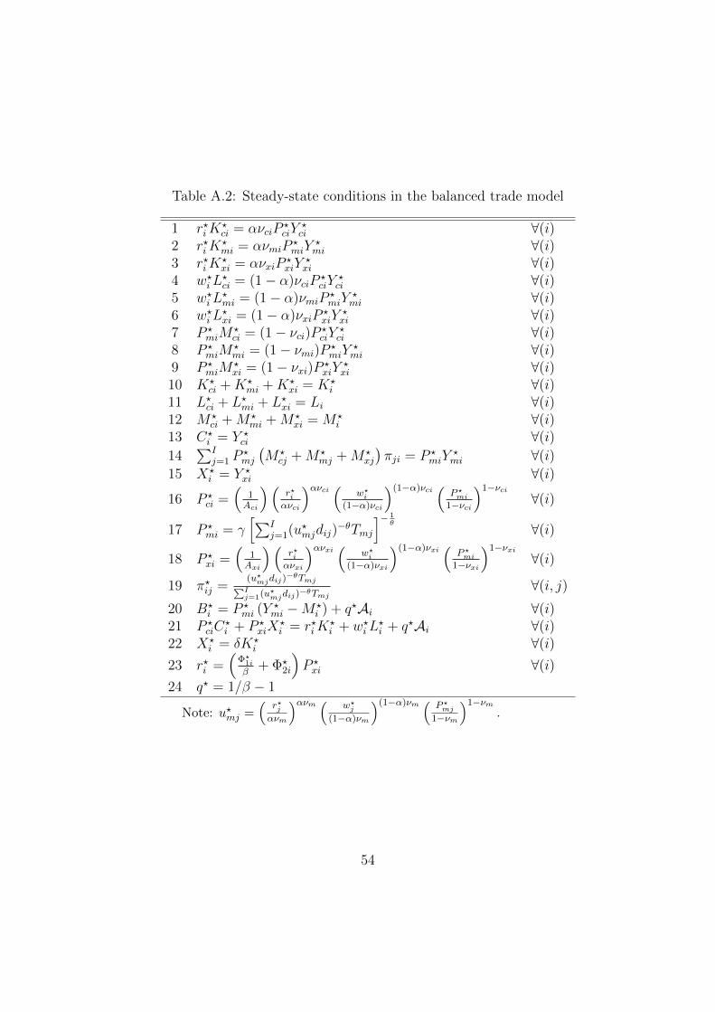
Table A.2: Steady-state conditions in the balanced trade model

1 r?iK?ci = ανciP

?ciY

?ci ∀(i)

2 r?iK?mi = ανmiP

?miY

?mi ∀(i)

3 r?iK?xi = ανxiP

?xiY

?xi ∀(i)

4 w?iL?ci = (1− α)νciP

?ciY

?ci ∀(i)

5 w?iL?mi = (1− α)νmiP

?miY

?mi ∀(i)

6 w?iL?xi = (1− α)νxiP

?xiY

?xi ∀(i)

7 P ?miM

?ci = (1− νci)P ?

ciY?ci ∀(i)

8 P ?miM

?mi = (1− νmi)P ?

miY?mi ∀(i)

9 P ?miM

?xi = (1− νxi)P ?

xiY?xi ∀(i)

10 K?ci +K?

mi +K?xi = K?

i ∀(i)11 L?ci + L?mi + L?xi = Li ∀(i)12 M?

ci +M?mi +M?

xi = M?i ∀(i)

13 C?i = Y ?

ci ∀(i)14

∑Ij=1 P

?mj

(M?

cj +M?mj +M?

xj

)πji = P ?

miY?mi ∀(i)

15 X?i = Y ?

xi ∀(i)

16 P ?ci =

(1Aci

)(r?iανci

)ανci ( w?i(1−α)νci

)(1−α)νci ( P ?mi1−νci

)1−νci∀(i)

17 P ?mi = γ

[∑Ij=1(u?mjdij)

−θTmj

]− 1θ ∀(i)

18 P ?xi =

(1Axi

)(r?iανxi

)ανxi ( w?i(1−α)νxi

)(1−α)νxi ( P ?mi1−νxi

)1−νxi∀(i)

19 π?ij =(u?mjdij)

−θTmj∑Ij=1(u?mjdij)

−θTmj∀(i, j)

20 B?i = P ?

mi (Y?mi −M?

i ) + q?Ai ∀(i)21 P ?

ciC?i + P ?

xiX?i = r?iK

?i + w?iL

?i + q?Ai ∀(i)

22 X?i = δK?

i ∀(i)23 r?i =

(Φ?1iβ

+ Φ?2i

)P ?xi ∀(i)

24 q? = 1/β − 1

Note: u?mj =(

r?jανm

)ανm ( w?j(1−α)νm

)(1−α)νm ( P ?mj1−νm

)1−νm.

54

Relative prices We show how to derive the price of consumption relative to inter-

mediates; the relative price of investment is analogous. Begin with condition 16 to obtain

Pci =

(Bci

Aci

)(riwi

)ανci ( wiPmi

)νciPmi,

where Bci is a collection of country-specific constants. Substitute equation (B.1) into the

previous expression and rearrange to obtain

PciPmi

=

(Bci

Aci

)(Tmiπii

) 1θ

γBmi

νciνmi

. (B.2)

Analogously,

PxiPmi

=

(Bxi

Axi

)(Tmiπii

) 1θ

γBmi

νxiνmi

. (B.3)

Note that these relationships hold in both the steady state and along the transition.

Income per worker We define (real) income per worker in our model as

yi =riKi + wiLi

LiPci.

We invoke conditions from Table A.1 for the remainder of this derivation. Conditions 1-6,

10, and 11 imply that

riKi + wiLi =wiLi1− α

⇒ yi =

(1

1− α

)(wiPci

).

To solve for wiPci

, we use condition 16:

Pci =Bci

Aci

(riwi

)ανci ( wiPmi

)νciPmi

⇒ Pciwi

=Bci

Aci

(riwi

)ανci ( wiPmi

)νci−1

.

55

Substituting equation (B.1) into the previous expression and exploiting the fact that wiri

=(1−αα

) (KiLi

)yields

yi =

(1

1− α

)(wiPci

)

= α−α (1− α)α−1

(AciBci

)(Tmiπii

) 1θ

Bmi

1−νciθνmi (

Ki

Li

)α. (B.4)

Steady-state capital-labor ratio and income We derive a structural relationship

for the capital-labor ratio in the steady state only and refer to conditions in Table A.2.

Conditions 1-6 together with conditions 10 and 11 imply that

Ki

Li=

(α

1− α

)(wiri

).

Using condition 23, we know that

ri =

(Φ1

β+ Φ2

)Pxi,

which, by substituting into the prior expression, implies that

Ki

Li=

α

(1− α)(

Φ1

β+ Φ2

)( wi

Pxi

),

which leaves the problem of solving for wiPxi

. Equations (B.1) and (B.3) imply

wiPxi

=

(wiPmi

)(PmiPxi

)

=

(AxiBxi

)(Tmiπii

) 1θ

γBmi

1−νxiνmi (

wiri

)α.

56

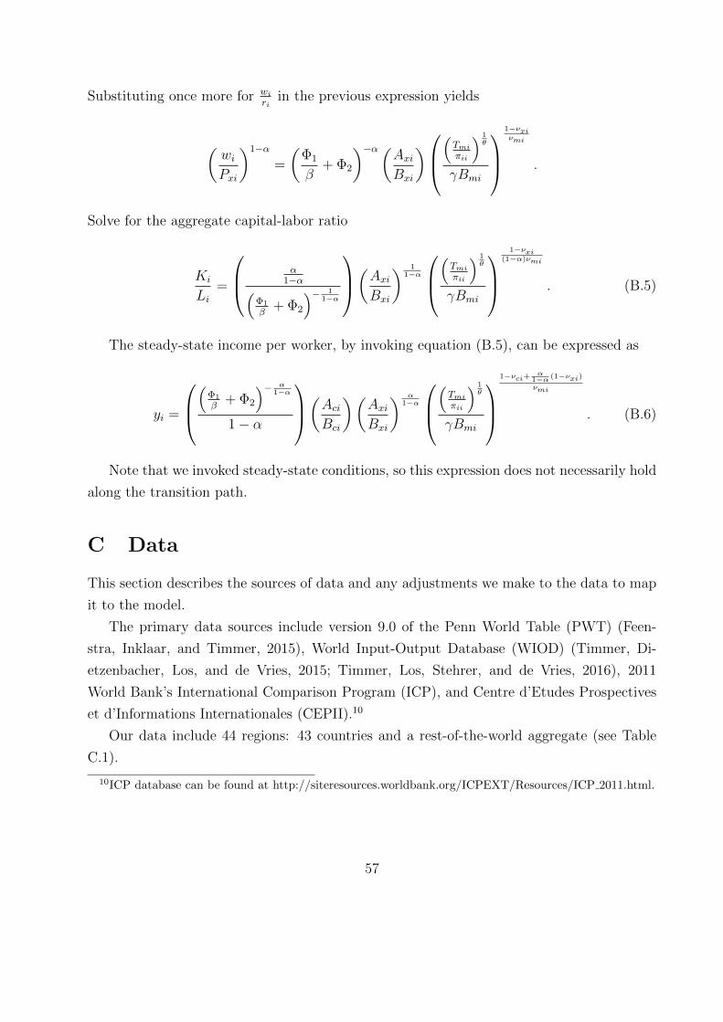
Substituting once more for wiri

in the previous expression yields

(wiPxi

)1−α

=

(Φ1

β+ Φ2

)−α(AxiBxi

)(Tmiπii

) 1θ

γBmi

1−νxiνmi

.

Solve for the aggregate capital-labor ratio

Ki

Li=

α1−α(

Φ1

β+ Φ2

)− 11−α

(AxiBxi

) 11−α

(Tmiπii

) 1θ

γBmi

1−νxi

(1−α)νmi

. (B.5)

The steady-state income per worker, by invoking equation (B.5), can be expressed as

yi =

(

Φ1

β+ Φ2

)− α1−α

1− α

(AciBci

)(AxiBxi

) α1−α

(Tmiπii

) 1θ

γBmi

1−νci+

α1−α (1−νxi)νmi

. (B.6)

Note that we invoked steady-state conditions, so this expression does not necessarily hold

along the transition path.

C Data

This section describes the sources of data and any adjustments we make to the data to map

it to the model.

The primary data sources include version 9.0 of the Penn World Table (PWT) (Feen-

stra, Inklaar, and Timmer, 2015), World Input-Output Database (WIOD) (Timmer, Di-

etzenbacher, Los, and de Vries, 2015; Timmer, Los, Stehrer, and de Vries, 2016), 2011

World Bank’s International Comparison Program (ICP), and Centre d’Etudes Prospectives

et d’Informations Internationales (CEPII).10

Our data include 44 regions: 43 countries and a rest-of-the-world aggregate (see Table

C.1).

10ICP database can be found at http://siteresources.worldbank.org/ICPEXT/Resources/ICP 2011.html.

57

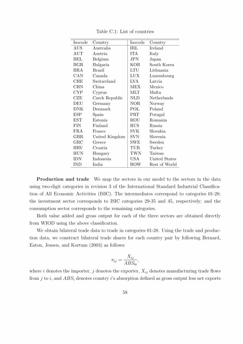
Table C.1: List of countries

Isocode Country Isocode Country

AUS Australia IRL IrelandAUT Austria ITA ItalyBEL Belgium JPN JapanBGR Bulgaria KOR South KoreaBRA Brazil LTU LithuaniaCAN Canada LUX LuxembourgCHE Switzerland LVA LatviaCHN China MEX MexicoCYP Cyprus MLT MaltaCZE Czech Republic NLD NetherlandsDEU Germany NOR NorwayDNK Denmark POL PolandESP Spain PRT PotugalEST Estonia ROU RomaniaFIN Finland RUS RussiaFRA France SVK SlovakiaGBR United Kingdom SVN SloveniaGRC Greece SWE SwedenHRV Croatia TUR TurkeyHUN Hungary TWN TaiwanIDN Indonesia USA United StatesIND India ROW Rest of World

Production and trade We map the sectors in our model to the sectors in the data

using two-digit categories in revision 3 of the International Standard Industrial Classifica-

tion of All Economic Activities (ISIC). The intermediates correspond to categories 01-28;

the investment sector corresponds to ISIC categories 29-35 and 45, respectively; and the

consumption sector corresponds to the remaining categories.

Both value added and gross output for each of the three sectors are obtained directly

from WIOD using the above classification.

We obtain bilateral trade data to trade in categories 01-28. Using the trade and produc-

tion data, we construct bilateral trade shares for each country pair by following Bernard,

Eaton, Jensen, and Kortum (2003) as follows:

πij =Xij

ABSbi,

where i denotes the importer, j denotes the exporter, Xij denotes manufacturing trade flows

from j to i, and ABSi denotes country i’s absorption defined as gross output less net exports

58

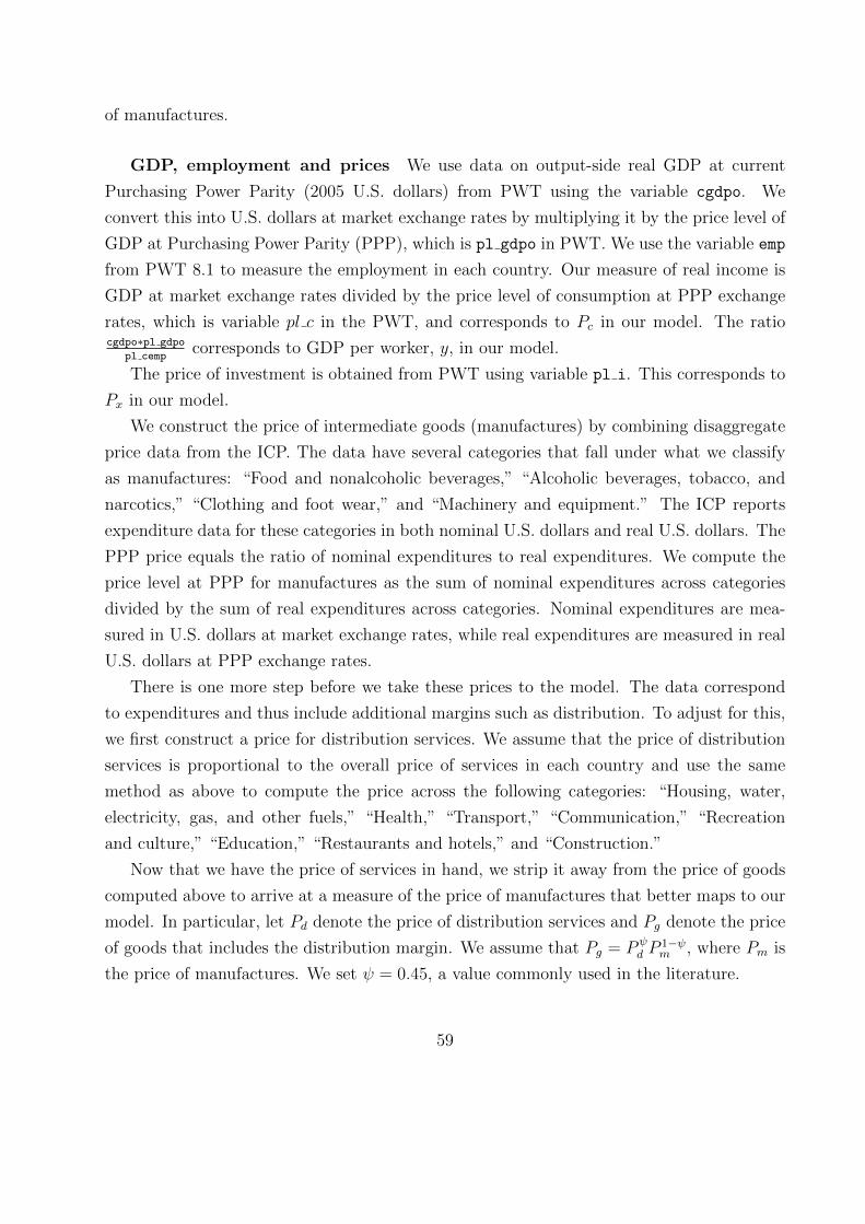
of manufactures.

GDP, employment and prices We use data on output-side real GDP at current

Purchasing Power Parity (2005 U.S. dollars) from PWT using the variable cgdpo. We

convert this into U.S. dollars at market exchange rates by multiplying it by the price level of

GDP at Purchasing Power Parity (PPP), which is pl gdpo in PWT. We use the variable emp

from PWT 8.1 to measure the employment in each country. Our measure of real income is

GDP at market exchange rates divided by the price level of consumption at PPP exchange

rates, which is variable pl c in the PWT, and corresponds to Pc in our model. The ratiocgdpo∗pl gdpo

pl cempcorresponds to GDP per worker, y, in our model.

The price of investment is obtained from PWT using variable pl i. This corresponds to

Px in our model.

We construct the price of intermediate goods (manufactures) by combining disaggregate

price data from the ICP. The data have several categories that fall under what we classify

as manufactures: “Food and nonalcoholic beverages,” “Alcoholic beverages, tobacco, and

narcotics,” “Clothing and foot wear,” and “Machinery and equipment.” The ICP reports

expenditure data for these categories in both nominal U.S. dollars and real U.S. dollars. The

PPP price equals the ratio of nominal expenditures to real expenditures. We compute the

price level at PPP for manufactures as the sum of nominal expenditures across categories

divided by the sum of real expenditures across categories. Nominal expenditures are mea-

sured in U.S. dollars at market exchange rates, while real expenditures are measured in real

U.S. dollars at PPP exchange rates.

There is one more step before we take these prices to the model. The data correspond

to expenditures and thus include additional margins such as distribution. To adjust for this,

we first construct a price for distribution services. We assume that the price of distribution

services is proportional to the overall price of services in each country and use the same

method as above to compute the price across the following categories: “Housing, water,

electricity, gas, and other fuels,” “Health,” “Transport,” “Communication,” “Recreation

and culture,” “Education,” “Restaurants and hotels,” and “Construction.”

Now that we have the price of services in hand, we strip it away from the price of goods

computed above to arrive at a measure of the price of manufactures that better maps to our

model. In particular, let Pd denote the price of distribution services and Pg denote the price

of goods that includes the distribution margin. We assume that Pg = Pψd P

1−ψm , where Pm is

the price of manufactures. We set ψ = 0.45, a value commonly used in the literature.

59

D Solution algorithm

In this appendix, we describe the algorithm for computing (i) the initial steady state and (ii)

the transition path. Before going further into the algorithms, we introduce some notation.

We denote the steady-state objects using the ? as a superscript; that is, K?i is the steady-

state stock of capital in country i. We denote the vector of capital stocks across countries

at time t as ~Kt = {Kit}Ii=1.

D.1 Computing the initial steady state

We use the technique from Mutreja, Ravikumar, and Sposi (2018), which builds on Alvarez

and Lucas (2007), to solve for the steady state. The idea is to guess a vector of wages, then

recover all remaining prices and quantities using optimality conditions and market-clearing

conditions, excluding the balance-of-payments condition. We then use departures from the

balance-of-payments condition in each country to update our wage vector and iterate until

we find a wage vector that satisfies the balance-of-payments condition. The following steps

outline our procedure in more detail:

(i) We guess a vector of wages ~w ∈ ∆ = {w ∈ RI+ :∑I

i=1wiLi1−α = 1}; that is, with world

GDP as the numeraire.

(ii) We compute prices ~Pc, ~Px, ~Pm, and ~r simultaneously using conditions 16, 17, 18, and 23

in Table A.2. The steady-state world interest rate is given condition 24. To complete

this step, we compute the bilateral trade shares ~~π using condition 19.

(iii) We compute the aggregate capital stock as Ki = α1−α

wiLiri

, for all i, which is easily

derived from optimality conditions 1 and 4, 2 and 5, and 3 and 6, coupled with market-

clearing conditions for capital and labor 10 and 11 in Table A.2.

(iv) We use condition 22 to solve for steady-state investment ~X. Then we use condition 21

to solve for steady-state consumption ~C.

(v) We combine conditions 4 and 13 to solve for ~Lc, combine conditions 5 and 14 to solve

for ~Lx, and use condition 11 to solve for ~Lm. Next we combine conditions 1 and 4

to solve for ~Kc, combine conditions 2 and 5 to solve for ~KM , and combine conditions

3 and 6 to solve for ~Kx. Similarly, we combine conditions 4 and 7 to solve for ~Mc,

combine conditions 5 and 8 to solve for ~Mm, and combine conditions 6 and 9 to solve

for ~Mx.

60

(vi) We compute ~Yc using condition 13, compute ~Ym using condition 14, and compute ~Yx

using condition 15.

(vii) We compute an excess demand equation as in Alvarez and Lucas (2007) defined as

Zi(~w) =PmiYmi − PmiMi + q?Ai

wi,

(the current account balance relative to the wage). Condition 20 requires that Zi(~w) =

0 for all i. If the excess demand is sufficiently close to 0, then we have a steady state.

If not, we update the wage vector using the excess demand as follows:

Λi(~w) = wi

(1 + ψ

Zi(~w)

Li

),

where ψ is chosen to be sufficiently small so that Λ > 0. Note that∑I

i=1Λi(~w)Li

1−α =∑Ii=1

wiLi1−α + ψ

∑Ii=1 wiZi(~w). As in Alvarez and Lucas (2007), it is easy to show that∑I

i=1 wiZi(~w) = 0 which implies that∑I

i=1Λi(~w)Li

1−α = 1, and hence, Λ : ∆→ ∆. We re-

turn to step (ii) with our updated wage vector and repeat the steps. We iterate through

this procedure until the excess demand is sufficiently close to 0. In our computations

we find that our preferred convergence metric,

Imaxi=1{|Zi(~w)|} ,

converges roughly monotonically towards 0.

D.2 Computing the transition path

The solution procedure boils down to two iterations. First, we guess a set of nominal

investment rates at each point in time for every country. Given these investment rates, we

adapt the algorithm of Sposi (2012) and iterate on the wages and the world interest rate

to pin down the endogenous trade imbalances. Then we go back and update the nominal

investment rates that satisfy the Euler equation for the optimal rate of capital accumulation.

To begin, we take the initial capital stock, Ki1, and the initial NFA position, Ai1, as

given in each country.

(i) Guess a path for nominal investment rates {~ρt}Tt=1 and terminal NFA, ~AT+1.

61

(ii) Guess the entire path for wages {~wt}Tt=1 and the world interest rate {qt}Tt=2, such that∑iwitLit1−α = 1 (∀t).

(iii) In period 1, set ~r1 =(

α1−α

) (~w1~L

~K1

)since the initial stock of capital is predetermined.

Compute prices Pc1, Px1, and Pm1 simultaneously using conditions 16, 17, and 18 in

Table A.1. Solve for investment, X1, using

Xit = ρitwitLit + ritKit

Pxit,

and then solve for the next-period capital stock, K2, using condition 22. Repeat this

set of calculations for period 2, then for period 3, and continue all the way through

period T . To complete this step, compute the bilateral trade shares {~~πt}Tt=1 using

condition 19.

(iv) Computing the path for consumption and bond purchases is slightly more involved.

This requires solving the intertemporal problem of the household. This is done in three

steps. First, we derive the lifetime budget constraint. Second, we derive the fraction

of lifetime wealth allocated to consumption in each period. And third, we recover the

sequences for bond purchases and the stock of NFAs.

Deriving the lifetime budget constraint To begin, (omitting country subscripts

for now) use the representative household’s period budget constraint in condition 20

and combine it with the NFA accumulation technology in condition 21 to get

At+1 = rtKt + wtLt − PctCt − PxtXt + (1 + qt)At.

Iterate the period budget constraint forward through time and derive a lifetime budget

constraint. At time t = 1, the NFA position, Ai1, is given. Next, compute the NFA

position at time t = 2:

A2 = r1K1 + w1L1 − Pc1C1 − Px1X1 + (1 + q1)A1.

62

Similarly, compute the NFA position at time t = 3, but do it so that it is in terms of

the initial NFA position.

A3 = r2K2 + w2L2 − Pc2C2 − Px2X2 + (1 + q2)A2

⇒ A3 = r2K2 + w2L2 − Px2X2 + (1 + q2)(r1K1 + w1L1 − Px1X1)

− Pc2C2 − (1 + q2)Pc1C1 + (1 + q2)(1 + q1)Ai1.

Continue to period 4 in a similar way:

A4 = r3K3 + w3L3 − Pc3C3 − Px3X3 + (1 + q3)A3

⇒ A4 = r3K3 + w3L3 − Px3X3

+ (1 + q3)(r2K2 + w2L2 − Px2X2)

+ (1 + q3)(1 + q2)(r1K1 + w1L1 − Px1X1)

− Pc3C3 − (1 + q3)Pc2C2 − (1 + q3)(1 + q2)Pc1C1 + (1 + q3)(1 + q2)(1 + q1)A1.

Before proceeding, it will be useful to define (1 +Qt) ≡∏t

n=1 (1 + qn):

⇒ A4 =(1 +Q3)(r3K3 + w3L3 − Px3X3)

(1 +Q3)

+(1 +Q3)(r2K2 + w2L2 − Px2X2)

(1 +Q2)

+(1 +Q3)(r1K1 + w1L1 − Px1X1)

(1 +Q1)

− (1 +Q3)Pc3C3

(1 +Q3)

− (1 +Q3)Pc2C2

(1 +Q2)

− (1 +Q3)Pc1C1

(1 +Q1)

+ (1 +Q3)A1.

63

By induction, for any time t,

At+1 =t∑

n=1

(1 +Qt)(rnKn + wnLn − PxnXn)

(1 +Qn)−

t∑n=1

(1 +Qt)PcnCn(1 +Qn)

+ (1 +Qt)A1

⇒ At+1 = (1 +Qt)

(t∑

n=1

rnKn + wnLn − PxnXn

(1 +Qn)−

t∑n=1

PcnCn(1 +Qn)

+A1

).

Finally, observe the previous expression as of t = T and rearrange terms to derive the

lifetime budget constraint:

T∑n=1

PcnCn(1 +Qn)

=T∑n=1

rnKn + wnLn − PxnXn

(1 +Qn)+A1 −

AT+1

(1 +QT )︸ ︷︷ ︸W

. (D.1)

In the lifetime budget constraint (D.1), W denotes the net present value of lifetime

wealth, taking both the initial and terminal NFA positions as given.

Solving for the path of consumption Next, compute how the net present value

of lifetime wealth is optimally allocated over time. The Euler equation (condition 24)

implies the following relationship between consumption in any two periods t and n:

Cn =

(LnLt

)βσ(n−t)

(1 +Qn1 +Qt

)σ (PctPcn

)σCt

⇒ PcnCn1 +Qn

=

(LnLt

)βσ(n−t)

(1 +Qn1 +Qt

)σ−1(PctPcn

)σ−1PtCt

1 +Qt.

Since equation (D.1) implies that∑T

n=1PcinCin1+Qn = W , rearrange the previous expression

(putting country subscripts back in) to obtain

PcitCit1 +Qit

=

(Litβ

σt(1 +Qit)σ−1P 1−σcit∑T

n=1 Linβσn(1 +Qin)σ−1P 1−σ

cin

)︸ ︷︷ ︸

ξit

Wi. (D.2)

That is, in each period, the household spends a share ξit of lifetime wealth on con-

sumption, with∑T

t=1 ξit = 1 for all i. Note that ξit depends only on prices.

64

Computing bond purchases and the NFA positions In period 1, take as given

consumption spending, investment spending, capital income, labor income, and net

income from the initial NFA position to solve for net bond purchases { ~Bt}Tt=1 using

the period budget constraint in condition 20. Solve for the NFA position in period

2 using condition 21. Then given income and spending in period 2, recover the net

bond purchases in period 2 and compute the NFA position for period 3. Continue this

process through all points in time.

Trade balance condition We impose that net exports equal the current account

less net foreign income from asset holding. That is,

Zwit

({~wt, qt}Tt=1

)=PmitYmit − PmitMit −Bit + qtAit

wit.

Condition 25 requires that Zwit

({~wt, ~rt}Tt=1

)= 0 for all (i, t) in equilibrium. If this is

different from 0 in some country at some point in time, update the wages as follows.

Λwit

({~wt, qt}Tt=1

)= wit

(1 + ψ

Zwit

({~wt, qt}Tt=1

)Lit

)

is the updated wages, where ψ is chosen to be sufficiently small so that Λw > 0.

Normalizing model units The next part of this step is updating the equilibrium

world interest rate. Recall that the numeraire is world GDP at each point in time:∑Ii=1(ritKit + witLit) = 1 (∀t). For an arbitrary sequence of {qt+1}Tt=1, this condition

need not hold. As such, update the world interest rate as

1 + qt =

∑Ii=1(rit−1Kit−1 + Λw

it−1Lit−1)∑Ii=1(ritKit + Λw

itLit)for t = 2, . . . , T. (D.3)

The capital and the rental rate are computed in step (ii), while the wages are the values

Λw above. The world interest rate in the initial period, q1, has no influence on the

model other than scaling the initial NFA position q1Ai1; that is, it is purely nominal.

We set q1 = 1−ββ

(the interest rate that prevails in a steady state) and choose Ai1 so

that q1Ai1 matches the desired initial NFA position in current prices.

Having updated the wages and the world interest rate, return to step (ii) and perform

65

each step again. Iterate through this procedure until the excess demand is sufficiently

close to 0. In the computations, we find that our preferred convergence metric,

Tmaxt=1

{I

maxi=1

{|Zw

it

({~wt, qt}Tt=1

)|}}

,

converges roughly monotonically toward 0. This provides the solution to a “sub-

equilibrium” for an exogenously specified nominal investment rate.

(v) The last step of the algorithm is to update the nominal investment rate and terminal

NFA condition. Until now, the Euler equation for investment in capital, condition 23,

has not been used. We compute an “Euler equation residual” as

Zrit

({~ρt}Tt=1

)= βσ

( rit+1

Pxit+1− Φ2(Kit+2, Kit+1)

Φ1(Kit+1, Kit)

)σ (Pxit+1/Pcit+1

Pxit/Pcit

)σ−(Cit+1

Cit

).

(D.4)

Condition 23 requires that Zrit

({~ρt}Tt=1

)= 0 for all (i, t) in equilibrium. We update the

nominal investment rates as

Λrit

({~ρt}Tt=1

)= ρit

(1 + ψZr

it

({~ρt}Tt=1

)). (D.5)

To update ρiT , we need to define Φ2(KiT+2, KiT+1), which is simply its steady-state

value, Φ?2 = δ − 1

λ, which serves as a boundary condition for the transition path of

capital stocks.

Given the updated sequence of nominal investment rates, return to step (i) and repeat.

Continue iterationing until maxTt=1

{maxIi=1

{|Zr

it

({~ρt}Tt=1

)|}}

is sufficiently close to 0.

Since the steady state cannot be determined independently from the transition path,

we need to update our guess for the terminal (steady state) NFA position AiT+1. In

our first iteration, we do not know what the steady state value is, so we set it equal

to 0. Given that initial guess, that first iteration is going to deliver a sequence of NFA

positions that, by the turnpike theorem, will converge to its steady-state value at some

time t? < T . After our first iteration, we take the NFA position at t? and use it as the

terminal condition for our second iteration. We choose t? as T × floor(

iterations1+iterations

).

In our algorithm we use T = 150 so that in iteration 2, t? = 100. This way of updating

the terminal NFA position ensures that the model settles down to its steady state

before and through T .

66

Our algorithm takes advantage of excess demand equations for our updating rules, just as

in Alvarez and Lucas (2007). One advantage of using excess demand iteration is that we

do not need to compute gradients to choose step directions or step size, as in the case of

nonlinear solvers such as the ones used by Eaton, Kortum, Neiman, and Romalis (2016) and

Kehoe, Ruhl, and Steinberg (2016). This saves a tremendous amount of computational time,

particularly as the number of countries or the number of time periods is increased.

E The role of capital: A static model

In calibrating the static model, we need to take a position on how we map the static model

to the data since capital stock is fixed and does not depend on tradables. The intermediate

goods sector is unchanged. That is, the tradables intensity in the intermediate goods sector,

νsmi = νmi (see equation 16). We combine consumption and investment goods sectors and

interpret the combination as one final good sector. That is, νsci is the ratio of sum of value

added of consumption and investment goods to the sum of gross output of consumption and

investment goods in country i. Figure E.1 illustrates νci for the static model and for the

baseline calibration in Section 3. Recall that νci in the restricted dynamic model is the same

as in the baseline calibration. The tradables intensity in consumption goods is higher in the

static model relative to the baseline model for practically every country in our sample.

We then calibrate productivities and trade costs to match income per worker, the price

of intermediates relative to consumption, and trade shares, as in Section 3. Note that the

trade costs in the static model are the same as in our baseline model since the structural

equation used to calibrate the trade costs in the static model is also equation (5) and the

data are the same. Finally, the initial capital stock is taken directly from the data, as in the

baseline calibration.

F Non-uniform trade liberalization

Our previous counterfactuals considered uniform reductions in trade frictions across coun-

tries. In practice these trade frictions include policy-induced impediments to trade as well as

frictions not directly influenced by policy, such as geography. Most trade liberalizations in-

volve reducing the policy-induced impediment to trade and, since the relative importance of

this component is heterogeneous across countries, these trade liberalizations are non-uniform.

We consider a counterfactual trade liberalization in which we remove the policy-induced im-

67

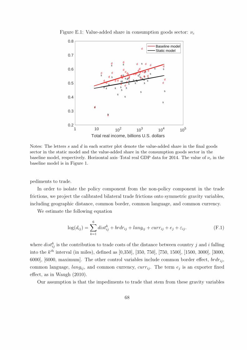
Figure E.1: Value-added share in consumption goods sector: νc

1 10 102 103 104 105

Total real income, billions U.S. dollars

0.2

0.3

0.4

0.5

0.6

0.7

0.8

dd

dd

d

d

d

d

d

d

d

d

d

d

d

d

d

d

dd

d

d

d

d

d

d

d

d

d

d

d

dd

d

d

dd

d

dd

dd

dd

ss

s

s

s

s

s

s

s

s

ss

s

s

s

ss

s

s

s

s

s

s

s

s

s

s

s

s

s

s

ss

s

s

ss

s

s

s

ss

s

s

Baseline modelStatic model

Notes: The letters s and d in each scatter plot denote the value-added share in the final goodssector in the static model and the value-added share in the consumption goods sector in thebaseline model, respectively. Horizontal axis–Total real GDP data for 2014. The value of νc in thebaseline model is in Figure 1.

pediments to trade.

In order to isolate the policy component from the non-policy component in the trade

frictions, we project the calibrated bilateral trade frictions onto symmetric gravity variables,

including geographic distance, common border, common language, and common currency.

We estimate the following equation

log(dij) =6∑

k=1

distkij + brdrij + langij + currij + ej + εij. (F.1)

where distkij is the contribution to trade costs of the distance between country j and i falling

into the kth interval (in miles), defined as [0,350], [350, 750], [750, 1500], [1500, 3000], [3000,

6000], [6000, maximum]. The other control variables include common border effect, brdrij,

common language, langij, and common currency, currij. The term ej is an exporter fixed

effect, as in Waugh (2010).

Our assumption is that the impediments to trade that stem from these gravity variables

68

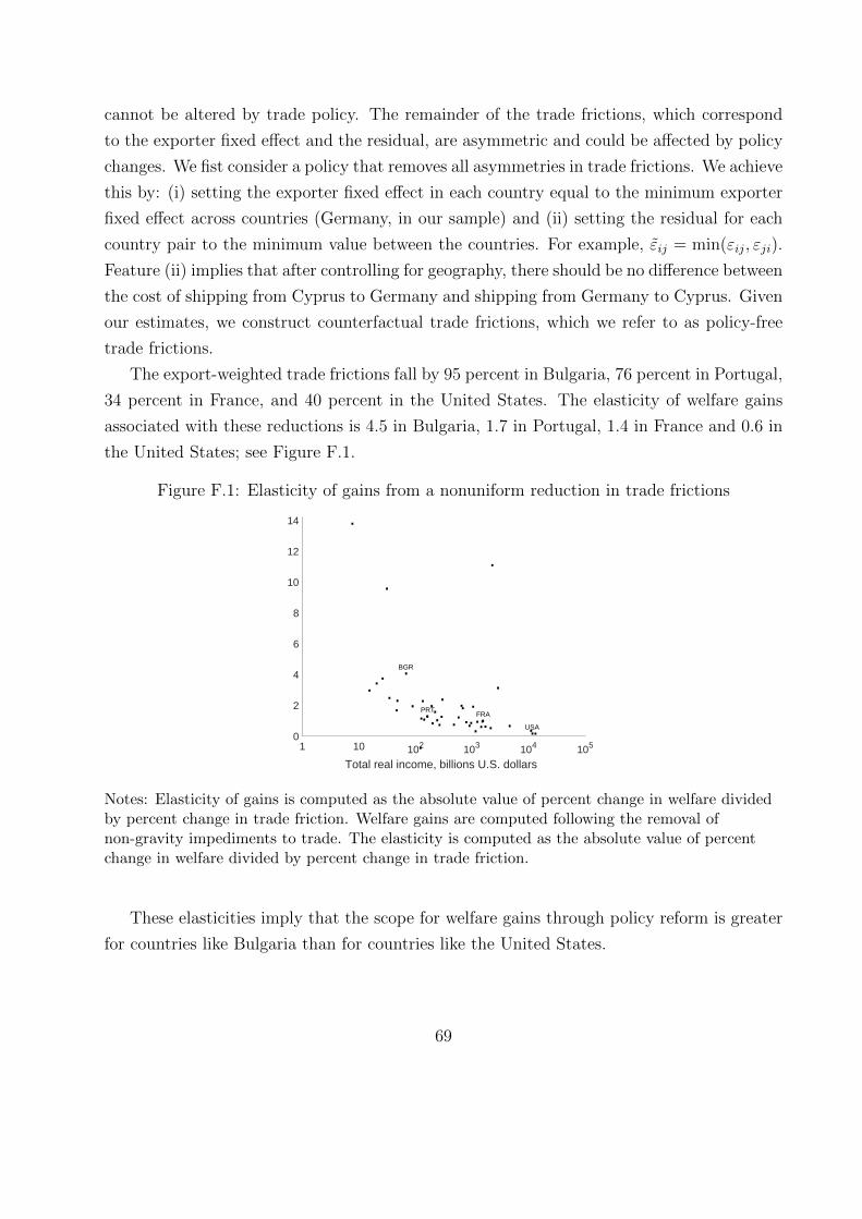
cannot be altered by trade policy. The remainder of the trade frictions, which correspond

to the exporter fixed effect and the residual, are asymmetric and could be affected by policy

changes. We fist consider a policy that removes all asymmetries in trade frictions. We achieve

this by: (i) setting the exporter fixed effect in each country equal to the minimum exporter

fixed effect across countries (Germany, in our sample) and (ii) setting the residual for each

country pair to the minimum value between the countries. For example, εij = min(εij, εji).

Feature (ii) implies that after controlling for geography, there should be no difference between

the cost of shipping from Cyprus to Germany and shipping from Germany to Cyprus. Given

our estimates, we construct counterfactual trade frictions, which we refer to as policy-free

trade frictions.

The export-weighted trade frictions fall by 95 percent in Bulgaria, 76 percent in Portugal,

34 percent in France, and 40 percent in the United States. The elasticity of welfare gains

associated with these reductions is 4.5 in Bulgaria, 1.7 in Portugal, 1.4 in France and 0.6 in

the United States; see Figure F.1.

Figure F.1: Elasticity of gains from a nonuniform reduction in trade frictions

1 10 102 103 104 105

Total real income, billions U.S. dollars

0

2

4

6

8

10

12

14

...

BGR.

...

.

..

.

. .

.

. FRA.... .

. ..

.

...

.

.

.

.

.. .PRT. ...

... .

.USA.

Notes: Elasticity of gains is computed as the absolute value of percent change in welfare dividedby percent change in trade friction. Welfare gains are computed following the removal ofnon-gravity impediments to trade. The elasticity is computed as the absolute value of percentchange in welfare divided by percent change in trade friction.

These elasticities imply that the scope for welfare gains through policy reform is greater

for countries like Bulgaria than for countries like the United States.

69

G Model with heterogeneous input-output linkages

We enrich our baseline model by incorporating a complete IO structure across four sectors.

This builds on Caliendo and Parro (2015) where every sector’s output goes into intermediate

and final use. Different from Caliendo and Parro (2015), the final use is split into con-

sumption and investment, thereby introducing dynamics via capital accumulation. We also

introduce one-period bonds to allow for endogenous trade imbalances and current account

dynamics.

Countries are indexed by (i, j) = 1, . . . , I, sectors by (n, k) = 1, . . . , N , and time by

t = 1, . . . , T . There are four sectors: durable goods, non-durable goods, durable services,

and non-durable services. In each sector, there is a continuum of varieties that are tradable.

Trade in varieties is subject to iceberg costs. Each country has a representative household

that owns the country’s primary factors of production, capital, and labor. Capital and labor

are mobile across sectors within a country but are immobile across countries. The household

inelastically supplies capital and labor to domestic firms, and it purchases output from each

sector and allocates it toward consumption and investments. Investment augments the stock

of capital. Households can trade one-period bonds so that trade imbalances are endogenous.

There is no uncertainty and households have perfect foresight.

Endowments The representative household in country i is endowed with workforce Li,

which is constant over time. In each period, households supply labor inelastically. In period

1 the household in country i is endowed with an initial stock of capital, Ki1, and an initial

NFA position, Ai1. These stocks evolve endogenously throughout time based on investment

and saving decisions.

Technology There is a unit interval of potentially tradable varieties in each sector

indexed by vn ∈ [0, 1] for n = 1, . . . , N .

Within each sector, country i bundles all of the varieties with constant elasticity in order

to construct a sectoral composite good according to

Qnit =

[∫ 1

0

Qnit(v

j)1−1/ηdvn]η/(η−1)

,

where η is the elasticity of substitution between any two varieties. The term Qnit(v

n) is the

quantity of variety vn used by country i at time t, which can be either imported or purchased

70

domestically, to construct the sector n composite good. The composite good, Qnit, is allocated

for domestic use as either an intermediate input or for final consumption or final investment.

Each variety can be produced using capital, labor, and composite goods. The technologies

for producing each variety in each sector are given by

Y nit (v

n) = zni (vn)(AniK

nit(v

n)αLnit(vn)1−α)νni ( N∏

k=1

Mnkit (vn)µ

nki

)1−νni

.

The term Mnkit (vn) denotes the quantity of the composite good of type k used by country i

to produce ynit(vn) units of variety vn in sector n at time t. Kn

it(vn) denotes the amount of

capital stock used and Lnit(vn) denotes the amount of workers employed.

The country-specific parameter νni ∈ [0, 1] is the share of value added in total output in

sector n, while µnki ∈ [0, 1] is the share of composite good k in total spending on intermediates

by producers in sector n, with∑

k µnki = 1. The term α denotes capital’s share in value added,

which is constant across sectors and across countries. All of these parameters are constant

over time.

The term Ani is the fundamental productivity, which scales value added, of all varieties

in sector n of country i. The term zni (vn) scales gross-output of variety vn in sector n of

country i. Following Eaton and Kortum (2002), gross-output productivity in sector n for

each variety is drawn independently from a Frechet distribution with sector-specific shape

parameter θn. The c.d.f. for idiosyncratic productivity draws in sector n in country i is

F n(z) = exp(−z−θn).

Preferences The representative household’s preferences are defined over consumption

per worker, {Cit/Li}Tt=1:

Ui =T∑t=1

βt−1

(CitLi

)1−1/σ

1− 1/σ.

Utility between adjacent periods is discounted by β ∈ (0, 1).

Consumption in country i at time t, Cit, bundles the consumption of composite goods

from all sectors according to

Cit =N∏n=1

(Cnit)ωcni ,

where Cnit denotes consumption of the sector n composite good by country i at time t, and

ωcni denotes sector n’s weight in the country i’s consumption bundle (i.e.,∑N

n=1 ωcni = 1).

71

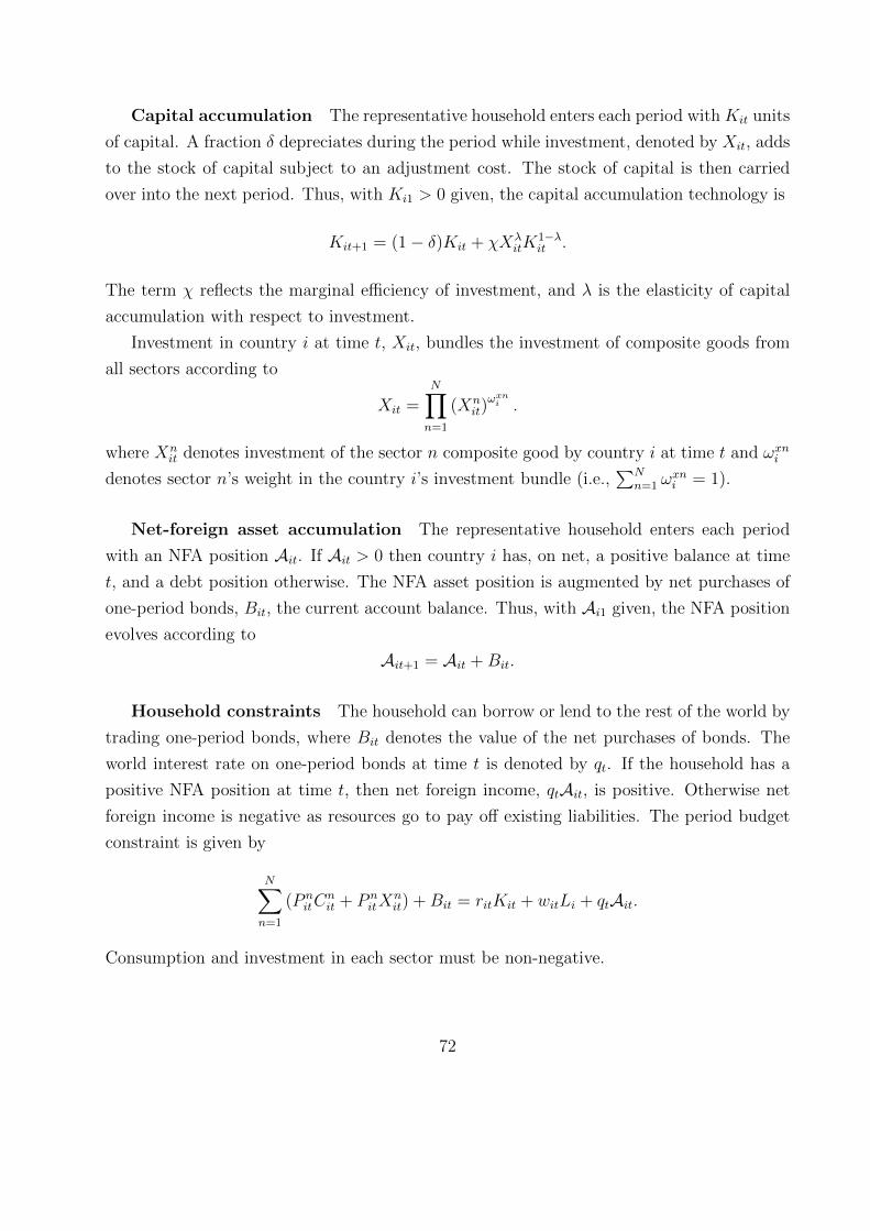
Capital accumulation The representative household enters each period with Kit units

of capital. A fraction δ depreciates during the period while investment, denoted by Xit, adds

to the stock of capital subject to an adjustment cost. The stock of capital is then carried

over into the next period. Thus, with Ki1 > 0 given, the capital accumulation technology is

Kit+1 = (1− δ)Kit + χXλitK

1−λit .

The term χ reflects the marginal efficiency of investment, and λ is the elasticity of capital

accumulation with respect to investment.

Investment in country i at time t, Xit, bundles the investment of composite goods from

all sectors according to

Xit =N∏n=1

(Xnit)

ωxni .

where Xnit denotes investment of the sector n composite good by country i at time t and ωxni

denotes sector n’s weight in the country i’s investment bundle (i.e.,∑N

n=1 ωxni = 1).

Net-foreign asset accumulation The representative household enters each period

with an NFA position Ait. If Ait > 0 then country i has, on net, a positive balance at time

t, and a debt position otherwise. The NFA asset position is augmented by net purchases of

one-period bonds, Bit, the current account balance. Thus, with Ai1 given, the NFA position

evolves according to

Ait+1 = Ait +Bit.

Household constraints The household can borrow or lend to the rest of the world by

trading one-period bonds, where Bit denotes the value of the net purchases of bonds. The

world interest rate on one-period bonds at time t is denoted by qt. If the household has a

positive NFA position at time t, then net foreign income, qtAit, is positive. Otherwise net

foreign income is negative as resources go to pay off existing liabilities. The period budget

constraint is given by

N∑n=1

(P nitC

nit + P n

itXnit) +Bit = ritKit + witLi + qtAit.

Consumption and investment in each sector must be non-negative.

72

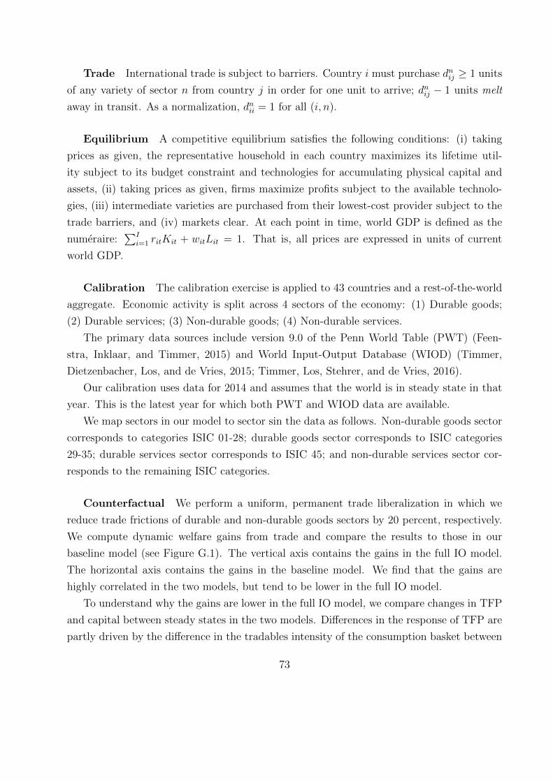
Trade International trade is subject to barriers. Country i must purchase dnij ≥ 1 units

of any variety of sector n from country j in order for one unit to arrive; dnij − 1 units melt

away in transit. As a normalization, dnii = 1 for all (i, n).

Equilibrium A competitive equilibrium satisfies the following conditions: (i) taking

prices as given, the representative household in each country maximizes its lifetime util-

ity subject to its budget constraint and technologies for accumulating physical capital and

assets, (ii) taking prices as given, firms maximize profits subject to the available technolo-

gies, (iii) intermediate varieties are purchased from their lowest-cost provider subject to the

trade barriers, and (iv) markets clear. At each point in time, world GDP is defined as the

numeraire:∑I

i=1 ritKit + witLit = 1. That is, all prices are expressed in units of current

world GDP.

Calibration The calibration exercise is applied to 43 countries and a rest-of-the-world

aggregate. Economic activity is split across 4 sectors of the economy: (1) Durable goods;

(2) Durable services; (3) Non-durable goods; (4) Non-durable services.

The primary data sources include version 9.0 of the Penn World Table (PWT) (Feen-

stra, Inklaar, and Timmer, 2015) and World Input-Output Database (WIOD) (Timmer,

Dietzenbacher, Los, and de Vries, 2015; Timmer, Los, Stehrer, and de Vries, 2016).

Our calibration uses data for 2014 and assumes that the world is in steady state in that

year. This is the latest year for which both PWT and WIOD data are available.

We map sectors in our model to sector sin the data as follows. Non-durable goods sector

corresponds to categories ISIC 01-28; durable goods sector corresponds to ISIC categories

29-35; durable services sector corresponds to ISIC 45; and non-durable services sector cor-

responds to the remaining ISIC categories.

Counterfactual We perform a uniform, permanent trade liberalization in which we

reduce trade frictions of durable and non-durable goods sectors by 20 percent, respectively.

We compute dynamic welfare gains from trade and compare the results to those in our

baseline model (see Figure G.1). The vertical axis contains the gains in the full IO model.

The horizontal axis contains the gains in the baseline model. We find that the gains are

highly correlated in the two models, but tend to be lower in the full IO model.

To understand why the gains are lower in the full IO model, we compare changes in TFP

and capital between steady states in the two models. Differences in the response of TFP are

partly driven by the difference in the tradables intensity of the consumption basket between

73

Figure G.1: Welfare gains from trade IO model and baseline model

0 5 10 15 20 25 30 35

2

4

6

8

10

AUS

AUT

BEL

BGR

BRA

CAN

CHE

CHN

CYP

CZE

DEU

DNK

ESP

EST

FIN

FRAGBR

GRC

HRV

HUN

IDN

IND

IRL

ITA

JPN

KOR

LTU

LUX

LVA

MEX

MLTNLD

NOR

POL

PRTROU

ROW

RUS

SVK

SVN

SWETUR

TWN

USA

Notes: Results following a uniform, 20 percent liberalization. Horizontal axis-Gains in thebaseline model. Vertical axis-Gains in the full IO model.

the two models. In the baseline model, the average tradables intensity of the consumption

basket is 1−νc = 0.44 and is ωc,DG+ωc,NG = 0.23 in the full IO model (G and DG correspond

to durable goods and non-durable goods). A larger tradables intensity in the baseline model

contributes to a larger response of TFP in that model. Figure G.2a shows that countries

that have a larger difference in this tradables intensity between the two models also have

a larger difference in the response of TFP. The steady-state change in TFP is defined as

the ratio between the counterfactual and the initial steady states. Similarly, differences in

the response of capital are partly driven by the difference in the tradables intensity in the

investment basket between the two models. In the baseline model, the average tradables

intensity of the investment basket is 1− νx = 0.67 and is ωx,DG +ωx,NG = 0.29 in the full IO

model. A larger tradables intensity in the baseline model contributes to a larger response

of capital in that model. Figure G.2b shows that countries that have a larger difference in

this tradables intensity between the two models, also have a larger difference in the response

of the capital stock. The steady-state change in the capital stock is defined as the ratio

between the counterfactual and the initial steady states.

74

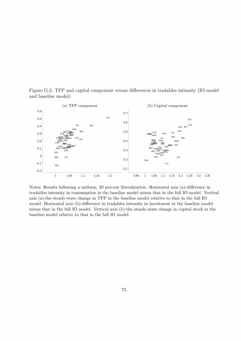
Figure G.2: TFP and capital component versus differences in tradables intensity (IO modeland baseline model)

(a) TFP component

1 1.05 1.1 1.15 1.2

-0.2

-0.1

0

0.1

0.2

0.3

0.4

0.5

0.6

AUSAUT

BEL

BGRBRA

CAN

CHE

CHN

CYP

CZE

DEU

DNK

ESP EST

FIN

FRA

GBR

GRC

HRV

HUN

IDN

IND

IRL

ITAJPN

KOR

LTU

LUX

LVA

MEX

MLT

NLDNOR

POL PRT

ROU

ROW

RUSSVKSVN

SWE

TUR

TWN

USA

(b) Capital component

0.95 1 1.05 1.1 1.15 1.2 1.25 1.3 1.35

0.1

0.2

0.3

0.4

0.5

0.6

0.7

AUS

AUT

BEL

BGR

BRA

CAN

CHE

CHN

CYP

CZE

DEU

DNK

ESPEST

FIN

FRA

GBR

GRCHRV

HUN

IDN

IND

IRL

ITA

JPN

KOR

LTU

LUX

LVA

MEX

MLT

NLDNOR

POL

PRT

ROU

ROW

RUS

SVK

SVN

SWE

TURTWN

USA

Notes: Results following a uniform, 20 percent liberalization. Horizontal axis (a)-difference intradables intensity in consumption in the baseline model minus that in the full IO model. Verticalaxis (a)-the steady-state change in TFP in the baseline model relative to that in the full IOmodel. Horizontal axis (b)-difference in tradables intensity in investment in the baseline modelminus that in the full IO model. Vertical axis (b)-the steady-state change in capital stock in thebaseline model relative to that in the full IO model.

75