welfare gains in a small open economy with a dual mandate
TRANSCRIPT

| T H E A U S T R A L I A N N A T I O N A L U N I V E R S I T Y
Crawford School of Public Policy
CAMA Centre for Applied Macroeconomic Analysis
Welfare gains in a small open economy with a dual mandate for monetary policy
CAMA Working Paper 89/2021 October 2021 Punnoose Jacob Reserve Bank of New Zealand Centre for Applied Macroeconomic Analysis, ANU Murat Özbilgin New Zealand Treasury
Abstract
In March 2019, the Reserve Bank of New Zealand was entrusted with a new employment stabilisation objective, that complements its traditional price-stability mandate. Against this backdrop, we assess whether the central bank’s stronger emphasis on the stabilisation of employment, and more broadly, resource utilisation, enhances social welfare. We calibrate an open-economy growth model to New Zealand data. In a second order approximation of the model, we evaluate how lifetime household utility is affected by a wide range of simple and implementable monetary policy rules that target both inflation and resource utilisation. We find that additionally stabilising resource utilisation always improves social welfare at any given level of inflation stabilisation. However, the welfare gains from stabilising resource utilisation get milder as the central bank is increasingly sensitive to inflation.

| T H E A U S T R A L I A N N A T I O N A L U N I V E R S I T Y
Keywords Optimal simple rules, welfare analysis, monetary policy, dual mandate JEL Classification F41, E52
Address for correspondence:
ISSN 2206-0332
The Centre for Applied Macroeconomic Analysis in the Crawford School of Public Policy has been
established to build strong links between professional macroeconomists. It provides a forum for quality
macroeconomic research and discussion of policy issues between academia, government and the private
sector.
The Crawford School of Public Policy is the Australian National University’s public policy school,
serving and influencing Australia, Asia and the Pacific through advanced policy research, graduate and
executive education, and policy impact.
Welfare gains in a small open economy with a dual
mandate for monetary policy*
Punnoose JacobReserve Bank of New Zealand and Centre for Applied Macroeconomic Analysis - ANU
Murat ÖzbilginNew Zealand Treasury
October 11, 2021
Abstract
In March 2019, the Reserve Bank of New Zealand was entrusted with a new employ-
ment stabilisation objective, that complements its traditional price-stability mandate.
Against this backdrop, we assess whether the central bank’s stronger emphasis on the
stabilisation of employment, and more broadly, resource utilisation, enhances social wel-
fare. We calibrate an open-economy growth model to New Zealand data. In a second-
order approximation of the model, we evaluate how lifetime household utility is affected
by a wide range of simple and implementable monetary policy rules that target both in-
flation and resource utilisation. We find that additionally stabilising resource utilisation
always improves social welfare at any given level of inflation stabilisation. However, the
welfare gains from stabilising resource utilisation get milder as the central bank is increas-
ingly sensitive to inflation.
JEL classification: F41, E52
Keywords: Optimal simple rules, welfare analysis, monetary policy, dual mandate
1 Introduction
Almost three decades after adopting inflation targeting as its principal objective, the mon-
etary policy framework of the Reserve Bank of New Zealand (RBNZ) underwent a paradigm
shift in March 2019. The new Monetary Policy Remit lays out the overarching goals of the
Monetary Policy Committee as “...maintaining a stable general level of prices over the medium
term and supporting maximum sustainable employment.” (RBNZ, 2019). Following this his-
toric amendment to the legislation, the RBNZ joined the Federal Reserve Bank of the United
*The views expressed herein are those of the authors, and do not necessarily represent the official views ofthe Reserve Bank of New Zealand or the New Zealand Treasury. We have benefitted from insightful comments byJames Graham, Vivien Lewis, Nicholas Sander, Dennis Wesselbaum as well as participants at the Reserve Bank-Treasury workshop on ’Fiscal and monetary policy in the wake of COVID’ in June 2021.
1
States and the Reserve Bank of Australia as the only central banks to be entrusted with a dual
mandate for monetary policy: an employment stabilisation objective coupled with the tradi-
tional price stability goal.1
This paper demonstrates that the second monetary policy objective of stabilising the
labour market - or in broader terms, resource utilisation - works to the benefit of society.
Using a medium-scale open-economy general equilibrium model calibrated to New Zealand
data, we find that additionally stabilising resource utilisation improves social welfare at any
given level of inflation stabilisation. The welfare gains from stabilising resource utilisation
are particularly striking when the response to inflation is weak. The second highlight of our
findings is that monetary policy responses to the labour market variables such as the em-
ployment gap or the unemployment rate gap, that are more in line with the activity indicators
stipulated in actual central bank legislation, yield better welfare outcomes than reacting to
the output gap. However, within the range of monetary policy settings we consider, the wel-
fare gains from stabilising resource utilisation decline to mild levels when the central bank is
already very sensitive to inflation.
The social desirability of stabilising resource utilisation is robust across a wide variety
of model specifications. The only exception is when the economy is driven solely by pow-
erful cost-push shocks to price and wage inflation that generate monetary policy trade-offs
between stabilising inflation and stabilising resource stabilisation. In this extreme case, we
find that the stabilisation of resource utilisation diminishes welfare, while strict inflation tar-
geting improves welfare. However, in the overall picture, when the business cycle is driven by
a wider range of demand-type and supply-type disturbances, the additional monetary policy
response to resource utilisation implied by the dual mandate enhances social welfare.
Our main findings for the open economy parallel the results of Debortoli, Kim, Lindé, and
Nunes (2019) who establish that placing a high weight on activity stabilisation in the central
bank’s loss function is optimal in the closed-economy model of Smets and Wouters (2007) for
the United States. Apart from the open-economy dimension of our model, our contribution
is quite distinct from their work in several other aspects. The legislative foundations for mon-
etary policy formulation in the United States, Australia and New Zealand direct the central
bank to target employment, rather than aggregate output which is the focus of Debortoli et al.
(2019). We explicitly model equilibrium unemployment. Finally, Debortoli et al. (2019) adopt
a linear-quadratic approach which involves the minimisation of a reduced-form central bank
loss function defined as a weighted combination of the volatilities of inflation and economic
activity, subject to a linear economy. In contrast, our assessment of welfare is in the tradition
established by Kollmann (2002) and Schmitt-Grohé and Uribe (2007). Using a second-order
1In the case of the United States, since 1977, the Federal Reserve has operated under a mandate from Congressto “...promote effectively the goals of maximum employment, stable prices, and moderate long term interest rates”(Steelman, 2011). In section 10(2) of the Reserve Bank Act 1959, the monetary policy mandate of the ReserveBank of Australia is to “...best contribute to: a. the stability of the currency of Australia; b. the maintenance of fullemployment in Australia; and c. the economic prosperity and welfare of the people of Australia.” (Reserve Bankof Australia, 2020). On the other hand, in Sweden, the Sveriges Riksbank Act 1988 states that the objective ofthe Riksbank’s monetary policy shall be to maintain price stability. The government bill that introduced the Actstates that “...the Riksbank shall also, without prejudice to the price-stability objective, support the objectives of thegeneral economic policy with the aim to achieve sustainable growth and high employment”. The Monetary PolicyReport of the Riksbank interprets the monetary policy mandate as ’flexible inflation targeting’ (Svensson, 2014).
2
approximation of the model around the non-stochastic steady state, we evaluate how the
household’s expected lifetime utility is affected by a set of simple and implementable mone-
tary policy rules; specifically, by systematically varying the response coefficients on inflation
and resource utilisation. Thus, unlike Debortoli et al. (2019), the welfare criterion that we
adopt is household utility rather than a reduced-form central bank loss function.2 However,
despite these numerous differences with the framework of Debortoli et al. (2019), the flavour
of the results remains similar: the stabilisation of resource utilisation - be it the employment
gap, the unemployment rate gap, or the output gap - by the central bank is beneficial for
society.
In modelling unemployment in the small open economy, our framework is similar to
that of Bodenstein, Kamber, and Thoenissen (2018) and Christiano, Trabandt, and Walentin
(2011). These authors use variants of the search-and-matching frictions in the tradition of
Mortensen and Pissarides (1994) to model unemployment. Unlike them, we choose the Galí
(2011) specification wherein nominal wage frictions give rise to equilibrium unemployment.
Corbo and Strid (2020) opt for a similar strategy in their estimated small open economy
model for Sweden. It is important to note that the other papers mentioned in this context
are positive in spirit, and hence use model solutions based on a first order approximation
around the steady state. In contrast, our paper assesses social welfare and as a consequence,
relies on the second order approximation of the model which, ceteris paribus, incorporates
a much more extensive model solution than the first order approximation. Since our small
open economy model already incorporates a rich array of other endogenous frictions, the
parsimony of the Galí (2011) specification of unemployment makes it particularly appealing.
Another aspect of our paper that links it to Kollmann (2002), besides the methodolog-
ical similarities, is the focus on the open economy. However, he considers a more limited
set of structural disturbances in a relatively smaller model whereas ours is a medium-scale
DSGE model that is a prototype of models used in central banks, and hence, is augmented
with a wider array of frictions and structural shocks. Kollmann (2002) also does not model
unemployment, and specifies only detrended output as the measure of resource utilisation
in the monetary policy rule. Since we model unemployment in our framework, we are able
to compare the performances of a triad of welfare-relevant measures of resource utilisation;
the gaps between output, employment or the unemployment rate and their analogues in a
counterfactual world without nominal rigidities.
Analysing the design of monetary policy using a second order approximation of the model,
also distinguishes our paper from a vast open-economy literature that instead adopts the
linear-quadratic approach. Some papers in this literature determine the monetary policy
settings that optimise a second order approximation of the utility function subject to lin-
earised competitive equilibrium conditions, as opposed to a second order approximation,
e.g. Corsetti, Dedola, and Leduc (2020, 2010), Fujiwara and Wang (2017) and De Paoli (2009).
Other authors minimise a reduced-form loss function that involves weighted combinations
2The part of the optimal policy analysis by Debortoli et al. (2019) that uses the estimated medium-scale modelof Smets and Wouters (2007) relies on the reduced-form loss function. They also demonstrate the relevance oftheir main result in the context of a second order approximation of household utility in a simplified version ofthe model, again using the linear-quadratic framework.
3
of the volatilities of target variables, again subject to a linearised economy, e.g. Jacob and
Munro (2018), Adolfson et al. (2014) and Justiniano and Preston (2010).
The rest of the paper will unfold as follows. In the next section, we lay out the structure
of the small open economy, and also explain our strategies for solving the model. In Sec-
tion 3, we present the welfare implications of altering the central bank responses to resource
utilisation and inflation. Section 4 evaluates the robustness of our baseline results, and high-
lights the extreme case in which powerful cost-push shocks drive the business cycle. We
summarise our conclusions in Section 5.
2 A small open economy model with unemployment
The world consists of two countries, the home country being infinitesimally small when
compared to the foreign country. We will refer to the home country as a small open economy
(SOE) and we will focus on deriving the optimality conditions for this region. The labour
market is set up in the spirit of Galí, Smets, and Wouters (2012) and Galí (2011). The open-
economy dimension of the model is based on Adolfson, Laséen, Lindé, and Villani (2007).
Hence, the exposition for these segments of the model closely follows that of the original
papers. As in Christiano, Trabandt, and Walentin (2011) and Mandelman, Rabanal, Rubio-
Ramirez, and Vilán (2011), the model incorporates permanent neutral and investment-specific
technical progress emanating from stochastic sources, and the model equations are later sta-
tionarised around a balanced growth path. The subscript t denotes the time period between
dates t and t+1, and Et denotes the conditional expectations operator. The steady-state val-
ues of the variables are denoted by an upper bar. Variables in the counterfactual economy
without nominal rigidities are indicated using a circumflex . The comprehensive derivation
of the model is presented in Jacob and Özbilgin (2021).
2.1 Production of intermediate goods
Three categories of firms operate in the SOE; domestic, importing and exporting firms. The
intermediate domestic firms produce a differentiated good, using capital and labour inputs,
which they sell to a final good producer who uses a continuum of these intermediate goods in
her production. The importing firms, in turn, transform a homogenous good, bought in the
world market, into a differentiated import good, which they sell to the domestic households.
The exporting firms pursue a similar scheme. The exporting firms buy the domestic final
good and differentiate it by brand naming. Each exporting firm is thus a monopoly supplier
of its specific product in the world market.
2.1.1 Domestic firms
The domestic firms are of two types. The first buys the aggregated labour (N) from the com-
petitive employment agencies at the nominal wage (W ) and rents the capital stock (K (s))
from the household at the nominal rate(Rk)
to produce intermediate goods (Y (s)) which it
sells to a final goods producer at a price (Pd(s)) . There is a continuum indexed by s ∈ [0, 1] of
4
these intermediate goods producers, each of which is a monopoly supplier of its own good
and is competitive in the markets for production inputs. The second type of firm transforms
the intermediate products into a homogenous final good, which is used for consumption
and investment by the households.
The production function of the final goods firm takes the form
Yt =
[� 1
0Yt (s)
(ξd,t−1)/ξd,t ∂s
]ξd,t/(ξd,t−1), ξd,t > 1 (1)
where ξd is a time-varying demand elasticity that follows the law of motion
ξd,t = ξ1−ρpdd ξ
ρpdd,t−1 expϑ
pdt , ρpd ∈ (0, 1) , ϑpd
t ∼ i.i.d.N (0, σpd ) . Profit-maximisation by the final
goods firm leads to the following first order condition
Yt (s) =
[Pd,t (s)
Pd,t
]−ξd,t
Yt, (2)
where Pd,t =[� 1
0 Pd,t (s)1−ςd,t ∂s
].
The intermediate goods firm s rents capital and labour from the household at the and
combines the two factors in a constant returns to scale Cobb-Douglas aggregate to produce
output.
Yt (s) = εneut [Kt−1 (s)]α [εatNt (s)]
1−α (3)
α ∈ [0, 1] governs the share of capital in the production function. εa is labour-augmenting
technological progress and its growth rate, defined as γat ≡ εat/εat−1, evolves according to
γat = (γa)1−ρa(γat−1
)ρa expϑat , ρa ∈ (0, 1) , ϑa
t ∼ i .i .d .N (0, σa) . The production function is
also stimulated by a stationary factor-neutral technology shock, εneu, which follows εneut =
(εneu)1−ρneu(εneut−1
)ρneu expϑneut , ρneu ∈ (0, 1) , ϑneu
t ∼ i .i .d .N (0, σneu) . Nominal rigidities in
price-setting are introduced using quadratic adjustment costs à la Rotemberg (1982); profits
are penalised when the change in the firm’s prices is different from a combination of lagged
aggregate inflation and steady-state inflation. Our decision to embed Rotemberg-type costs
instead of using staggered price-setting in the style of Calvo (1983) to model nominal rigidi-
ties is motivated by the presence of time-varying price elasticities in Equation 2 that gener-
ate exogenous movements in the price mark-up. However, as noted by Andreasen (2012),
a time-varying price elasticity or mark-up precludes an exact recursive formulation of the
Calvo price-setting equations necessary for the non-linear approximation of the model. The
Rotemberg (1982) specification is particularly convenient for us, given its compatibility with
time-varying elasticities of goods and labour demand in the non-linear model solution. Im-
portantly, as we will see in Section 4, the presence of time-varying elasticities that act as
cost-push shocks to price and wage inflation have important implications for the monetary
policy mandate.3
3Exogenous time-variation in price and wage elasticities are also found to be important driving forces of priceand wage inflation in standard empirical DSGE models, e.g. Smets and Wouters (2007) and Adolfson et al. (2007).Alternatively, as in Andreasen (2012), we could use Calvo-style price-setting by avoiding price elasticity shocksand instead, introducing shocks to fixed costs that are embedded in the production function. However, in thatcase, we would not have analogous shocks to the wage-setting problem detailed in Section 2.1.1; while Andreasen
5
The firm faces the following profit maximisation programme:
maxKt−1(s), Nt(s)
Pd,t(s)
Et
∞∑τ=0
βτ Λt+τ
Pc,t+τ
Pd,t+τ (s)Yt+τ (s)−Wt+τNt+τ (s)−Rkt+τKt+τ (s)
−χd2
(Pd,t+τ (s)
π1−ιdd π
ιdd,t+τ−1Pd,t+τ−1(s)
− 1
)2
Pd,t+τYt+τ
subject to the production technology constraint in Equation 3 and the demand constraint in
Equation 2. Λ is the marginal utility of income, Pc is the price of consumption and β ∈ (0, 1)
is the subjective discount factor. The parameters χd ≥ 0 measures the degree of costly price
adjustment and ιd ∈ [0, 1] indicates the degree of indexation to lagged inflation. We will focus
on the optimality conditions in a symmetric equilibrium where all firms set the same prices.
The optimal choice of labour and capital input yield
Wd,tNt = (1− α)RMCd,tYt, (4)
and
Rkd,tKt−1 = αRMCd,tYt, (5)
where Wd and Rkd are the respective factor payments deflated by the output deflator Pd. The
output-based real marginal cost is given as
RMCd,t =1
εneut αα (1− α)1−α
(Rk
d,t
)α(Wd,t
εat
)1−α
. (6)
Optimal price-setting implies that movements in the real marginal cost reflect in movements
in price inflation πd, with the price adjustment cost parameter moderating the strength of the
relationship:
πd,t
π1−ιdd πιd
d,t−1
χd
(πd,t
π1−ιdd πιd
d,t−1
− 1
)= (1− ξd,t) + ξd,tRMCd,t
+βEtΛt+1
Λtπc,t+1
Yt+1
Yt
π2d,t+1
π1−ιdd πιd
d,t
χd
(πd,t+1
π1−ιdd πιd
d,t
− 1
). (7)
2.1.2 Importing firms
The import sector consists of firms that buy a homogenous good in the world market at the
foreign-currency price P ∗. The imported good is absorbed by aggregator firms that produce
the final consumption and investment imported goods that are sold to the household. The
aggregator firms face the following production functions:
Cm,t =
[� 1
0Cm,t (s)
(ξm,t−1)/ξm,t ∂s
]ξm,t/(ξm,t−1)
(8)
(2012) abstracts from nominal wage rigidities, wage-setting frictions are crucial for introducing unemploymentinto our model. Quadratic adjustment costs allows us to model price- and wage-setting frictions symmetrically,even while retaining conventional shocks understood to be important drivers of the business cycle.
6
and
Im,t =
[� 1
0Im,t (s)
(ξm,t−1)/ξm,t ∂s
]ξm,t/(ξm,t−1)
, ξm,t > 1 (9)
where ξm is a time-varying demand elasticity that follows the law of motion
ξm,t = ξ1−ρpmm ξ
ρpmm,t−1 expϑ
pmt , ρpm ∈ (0, 1) , ϑpm
t ∼ i .i .d .N (0, σpm) . Profit-maximisation by
the perfectly competitive aggregator firms for consumption and investment imports yield
the following first order conditions:
Cm,t (s) =
[Pm,t (s)
Pm,t
]−ξm,t
Cm,t, (10)
and
Im,t (s) =
[Pm,t (s)
Pm,t
]−ξm,t
Im,t, (11)
where Pm,t =[� 1
0 Pm,t (s)1−ξm,t ∂s
]. The profit maximisation programme for the monopolis-
tic intermediate goods importer is given by
maxPm,t(s)
Et
∞∑τ=0
βτ Λt+τ
Pc,t+τ
Pm,t+τ (s)Cm,t+τ (s) + Pm,t+τ (s) Im,t+τ (s)
−χm
2
(Pm,t+τ (s)
π1−ιmm πιm
m,t+τ−1Pm,t+τ−1(s)− 1
)2
Pm,t+τ (Cm,t+τ + Im,t+τ )
−nert+τP∗t+τCm,t+τ (s)− nert+τP
∗t+τIm,t+τ (s)
χm ≥ 0, ιm ∈ [0, 1] ,
subject to the demand constraints in Equations 10 and 11. On the revenue side, the im-
porter’s profits are affected by the consumption and investment goods sold to the household
at the home currency-denominated import price. On the other hand, import costs are af-
fected by the nominal exchange rate ner that is defined as the home currency price of one
unit of foreign currency as the procurement price of the good is denominated in foreign
currency.4 In addition, profits are influenced by nominal import price rigidities that are
modelled using quadratic adjustment costs, analogous to the case of domestic sales pric-
ing that we presented earlier. We further define the output-based real exchange rate as
rerd ≡ nerPd/P∗ and the relative price of imports in terms of the price of home output as
rpmd ≡ Pm/Pd. The ratio of these two international relative prices represents the effective
real marginal cost of the importer. The optimality condition for import prices implies that
the presence of price rigidities moderate the pass-through of exchange rate fluctuations into
import price inflation.
πm,t
π1−ιmm πιm
m,t−1
χm
(πm,t
π1−ιmm πιm
m,t−1
− 1
)= (1− ξm,t) + ξm,t
rerd,trpmd,t
+βEtΛt+1
Λtπc,t+1
(Cm,t+1 + Im,t+1)
(Cm,t + Im,t)
π2m,t+1
π1−ιmm πιm
m,t
χm
(πm,t+1
π1−ιmm πιm
m,t
− 1
). (12)
4Hence, a rise in the exchange rate indicates a depreciation of the home currency.
7
2.1.3 Exporting firms
The exporting firms buy the final domestic good and differentiate it by brand naming, and
sell the continuum of differentiated goods to the households in the foreign market. The nom-
inal marginal cost is thus the price (Pd) of the domestic good. Each exporting firm s faces the
following demand for its product.
Yx,t(s) =
(Px,t(s)
Px,t
)−ξx,t
Yx,t, (13)
where Yx,t is the aggregate volume of exports from the SOE and Px,t(s)/Px,t is the price of
the individual exported variety to the aggregate export price. ξx,t is the elasticity of export
demand to the relative price which follows a stochastic process given as
ξx,t = ξ1−ρpxx ξ
ρpxx,t−1 expϑ
pxt , ρpx ∈ (0, 1) , ϑpx
t ∼ i .i .d .N (0, σpx ) . Since the exports are priced
in foreign currency, profits have to converted back to the SOE currency by using the nominal
exchange rate. Akin to the case of price-setting for domestic and import sales, export profits
are also diminished by quadratic adjustment costs. The profit maximisation programme is
given as
maxPx,t+τ (s)
Et
∞∑τ=0
βτ Λt+τ
Pc,t+τ
nert+τPx,t+τ (s)Yx,t+τ (s)− Pd,t+τYx,t+τ (s)
−χx
2
(Px,t+τ (s)
π1−ιxx πιx
x,t+τ−1Px,t+τ−1(s)− 1
)2
nert+τPx,t+τYx,t+τ
χx ≥ 0, ιx ∈ [0, 1] ,
subject to the constraint in Equation 13. We define the relative price of exports in terms of
the foreign price level as rpx = Px/P∗. The optimality condition for export prices suggests
that export price inflation covaries inversely with the effective foreign-currency price markup
rerdrpx ,
πx,t
π1−ιxx πιx
x,t−1
χx
(πx,t
π1−ιxx πιx
x,t−1
− 1
)= (1− ξx,t) +
ξx,trerd,trpxt
+βEtΛt+1
Λt
nert+1
nertπc,t+1
Yx,t+1
Yx ,t
π2x,t+1
π1−ιxx πιx
x,t
χx
(πx,t+1
π1−ιxx πιx
x,t
− 1
). (14)
Finally, the aggregate exports of the SOE to the foreign economy is given as
Yx,t = rpx−ηxY ∗t , (15)
where Yx,t is the volume of exports from the SOE, Y ∗t is foreign output, foreign price level and
ηx > 0 is the price elasticity of export demand.
2.2 Aggregation of goods
Final goods producers are assumed to be perfectly competitive. The final consumption and
investment goods (C, I) are assumed to be given by CES indices of domestically-produced
8
(Cd, Id) and imported goods (Cm, Im) according to
Ct =
[(1−mc)
1ηc C
ηc−1ηc
d,t +m1ηcc C
ηc−1ηc
m,t
] ηcηc−1
, mc ∈ [0, 1] , ηc > 0, (16)
and
It = εistt
[(1−mi)
1ηi I
ηi−1
ηid,t +m
1ηii I
ηi−1
ηim,t
] ηiηi−1
, mi ∈ [0, 1] , ηi > 0. (17)
As in Christiano, Trabandt, and Walentin (2011), εistt is an investment-specific technology
shock that stimulates the production of investment goods, and it follows a random walk with
drift. This implies that the growth rate of investment-specific technology defined as γistt ≡εistt /εistt−1 evolves according to the stationary process γistt =
(γist)1−ρist (γistt−1
)ρist expϑistt , ρist ∈
(0, 1) , ϑistt ∼ i .i .d .N (0, σist) . As noted in the earlier section, the prices of the domestic and
imported bundles are given by Pd and Pm respectively. The cost minimisation programmes
that faces the final goods producers for consumption and investment are respectively:
minCd,t, Cm,t
Pd,tCd,t + Pm,tCm,t
subject to Equation 16 and
minId,t, Im,t
Pd,tId,t + Pm,tIm,t
subject to Equation 17. Domestic sales are given as
Cd,t = (1−mc)
(Pd,t
Pc,t
)−ηc
Ct, Id,t = (1−mi)
(Pd,t
εistt Pi,t
)−ηi Itεistt
(18)
and import demand is derived as
Cm,t = mc
(Pm,t
Pc,t
)−ηc
Ct, Im,t = mi
(Pm,t
Pi,tεistt
)−ηi Itεistt
. (19)
The Lagrange multipliers associated with the above cost-minimisation programmes, i.e. the
aggregate price deflators for consumption (Pc) and investment (Pi), are combinations of the
domestic and import sales prices:
Pc,t =[(1−mc)P
1−ηcd,t +mcP
1−ηcm,t
] 11−ηc (20)
and
Pi,t =1
εistt
[(1−mi)P
1−ηid,t +miP
1−ηim,t
] 11−ηi . (21)
2.3 Household preferences and constraints
The model assumes a large representative household with a continuum of members repre-
sented by the unit square and indexed by a pair (i, j) ∈ [0, 1] × [0, 1]. The first dimension,
indexed by i ∈ [0, 1], represents the type of labour service in which a given household mem-
9
ber is specialised. The second dimension, indexed by j ∈ [0, 1], determines her disutility from
work. The latter is given by εltΘtjφn if she is employed and zero otherwise. εlt > 0 is a labour
supply shock which follows the law of motion εlt =(εl)1−ρl (εlt−1
)ρl expϑlt, ρl ∈ (0, 1) , ϑl
t ∼i .i .d .N (0, σl ) . Θt is a preference shifter that is taken as given by each individual household
and defined below, and φn ≥ 0 is a parameter determining the shape of the distribution of
work disutilities across individuals.
Individual utility in every period is assumed to be given by log Ct (i, j) − 1(i, j)εltΘtjφn ,
where Ct (i, j) ≡ Ct (i, j)− hcCt−1, with hc ∈ [0, 1] and Ct−1 denoting (lagged) aggregate con-
sumption taken as given by each household. 1(i, j) is an indicator function taking a value
equal to one if individual (i, j) is employed in period t and zero otherwise. In addition, con-
sumption risk is shared perfectly among household members, implying that in every period
Ct (i, j) = Ct for all (i, j) = Ct ∈ [0, 1] × [0, 1]. Thus, the utility of the household can be
expressed as the integral over its members’ utilities, that is:
Ut (Ct, Nt(i)) ≡ log Ct − εltΘt
1�
0
Nt(i)�
0
jφn∂j∂i
= log Ct − εltΘt
1�
0
Nt(i)1+φn
1 + φn∂i, (22)
where Nt(i) ∈ [0, 1] denotes the employment rate in period t among workers specialised in
type i labour and Ct (i, j) ≡ Ct − hcCt−1. The endogenous preference shifter Θt is defined as
Θt ≡Zt
Ct − hcCt−1
, (23)
where Zt evolves over time according to
Zt = Z1−vzt−1
(Ct − hcCt−1
)vz. (24)
Thus, Zt can be interpreted as a ’smooth’ trend for (quasi-differenced) aggregate consump-
tion. This preference specification implies a consumption externality on individual labour
supply: during aggregate consumption booms when habit-adjusted consumption rises above
trend, individual and household-level marginal disutility from work goes down, at any given
level of employment. The main role of the endogenous preference shifter Θt is to recon-
cile the existence of a long-run balanced growth path with an arbitrarily small short-term
wealth effect that is governed by the size of the parameter vz ∈ [0, 1]. The smaller is vz, the
wealth effect on labour supply declines, augmenting the positive comovement of the labour
force, consumption and the wage over the business cycle. Under these preferences, the
household-relevant marginal rate of substitution between consumption and employment
for type i workers in period t is given by:
MRSt(i) ≡ −UN(i),t/UC,t = εltΘtCtNt(i)φ = εltZtNt(i)
φ, (25)
10
where the last equality is satisfied in a symmetric equilibrium with Ct = Ct. As in Erceg,
Henderson, and Levin (2000), perfectly competitive ’employment agencies’ aggregate the
specialised labour-varieties (N(i)) from the households into a homogenous labour input (N)
using a constant elasticity of substitution technology, and sell it to the firm. The employment
agencies return to the household a labour-type specific nominal wage (W (i)). The demand
for the specific labour type from the employment agency is given as
Nt(i) =
(Wt(i)
Wt
)−ξn,t
Nt, (26)
and the elasticity of labour demand to the idiosyncratic wage relative to the aggregate wage
index (W ) is time-varying, and follows a stochastic process akin to that of analogous price
elasticities in the goods market: ξn,t = ξ1−ρnn ξρnn,t−1 expϑ
nt , ρn ∈ (0, 1) , ϑn
t ∼ i .i .d .N (0, σn) .We
position nominal wage-setting frictions, another crucial building block of the labour market
in the tradition of Galí et al. (2012) and Galí (2011), in the period budget constraint of the
household that we present in Equation 27.
Ct +Pi,t
Pc,tIt +
Bt
Pct+
nertNFAt
Pc,t=
� 10 Wt(i)Nt(i)∂i
Pc,t− WtNt
Pc,t
1�
0
χw
2
(Wt(i)
(πc,t−1γt−1)ιw (πcγ)
1−ιw Wt−1(i)− 1
)2
∂i
+Rk
t
Pc,tKt−1 +
Rt−1
Pc,tBt−1 +
nertR∗t−1Ξt−1
Pc,tNFAt−1 +
DIVt
Pc,t.
(27)
The household receives total wage income� 10 W (i)N(i)∂i from all its working members. Mir-
roring the nominal frictions that impede the price-setting decisions of firms that we pre-
sented in the previous section, we introduce nominal wage rigidities by stipulating that quadratic
adjustment costs à la Rotemberg (1982) reduce household income when it optimally chooses
the labour-type specific wage. In particular, when the growth of the idiosyncratic nom-
inal wage deviates from a combination of past headline inflation (πc,t−1) and trend eco-
nomic growth (γt−1) and their steady-state levels (πcγ). The parameter χw ≥ 0 measures the
strength of the penalty to income for a given deviation of the idiosyncratic wage inflation,
while the wage indexation parameter ιw ∈ [0, 1] quantifies the dependence of wage inflation
on lagged price inflation.5
The rest of the budget constraint is fairly standard. In every period, the household pur-
chases the final goods for consumption (C) and investment (I), private domestic currency-
denominated nominal bonds (B), and private foreign currency-denominated nominal bonds
(NFA). On the income side, nominal net returns(Rk)
are obtained from renting out physical
5Note that, unlike Galí et al. (2012) and Galí (2011), we do not use Calvo-style wage-setting. This is due to theincompatibility between the objective of deriving the recursive Calvo equations for our non-linear model solu-tion, with that of using the time-varying wage elasticity that we need to account for the implications of inefficientsupply shocks. In contrast, Galí et al. (2012) rely on a linearised model solution that combine a Calvo-style wagePhillips curve with time-varying wage markup shocks. See also Section 2.1.1 on price-setting for domestic salesand Footnote 3.
11
capital (Kt−1) to the firms in the previous period, gross nominal interest returns (Rt−1Bt−1)
from the domestic financial asset holdings and(nertR
∗t−1Ξt−1NFAt−1
)from the foreign fi-
nancial asset holdings, and finally, dividends (DIV ) that accrue to the households due to
its ownership of the firms. The gross interest rates Rt and R∗t are set by the SOE and the
foreign central banks. In the spirit of Adolfson et al. (2007), a risk premium term Ξt =
εuipt exp−κnfa
(nert ¨NFAt
Pd,tYt− ner ¨NFA
PdY
)is appended to the foreign interest rate. It has an en-
dogenous component so that the parameter κnfa > 0 governing its elasticity to the aggregate
stock of the foreign bonds ¨NFAt. This endogenous part of the risk premium ensures that the
incomplete markets model has a unique steady state and hence can be solved using standard
perturbation methods.6 The risk premium also has an exogenous component εuip that fol-
lows γuipt =(γuip
)1−ρuip(γuipt−1
)ρuipexpϑuip
t , ρuip ∈ (0, 1) , ϑuipt ∼ i .i .d .N (0, σuip) . Investment
is transformed to installed physical capital according to the law of motion
Kt = (1− δ)Kt−1 + εmeit
[It −
ϕinv
2It−1
(ItIt−1
− γinv
)2]. (28)
The new physical capital stock is the sum of the undepreciated capital stock, with δ ∈ [0, 1]
determining the rate of depreciation, and newly acquired investment goods. It is assumed
that the transformation of investment goods into physical capital is costly. The quadratic
cost function we use is adapted from Mandelman et al. (2011). If the adjustment cost param-
eter ϕinv > 0, the incurred cost rises with the gap betwen the growth rate of investment and
its steady-state value of γinv. Finally, as in Justiniano, Primiceri, and Tambalotti (2011), a sta-
tionary shock εmeit that stimulates the marginal efficiency of capital is assumed to affect cap-
ital accumulationm, and follows εmeit =
(εmei
)1−ρmei(εmeit−1
)ρmei expϑmeit , ρmei ∈ (0, 1) , ϑmei
t ∼i .i .d .N (0, σmei) . The optimisation programme that faces the household is:
maxBt, NFAt, Wt(i),
Ct, Kt, It
E0
∞∑t=0
βtεctU (Ct, Nt(i))
subject to Equations 26, 27, and 28. Along with these constraints, the optimisation pro-
gramme is supplemented with an end-point restriction for asset holdings, so that the house-
hold does not engage in Ponzi schemes.
As in the case of firms, we will focus on a symmetric equilibrium. The optimal choice of
consumption implies an inverse relation between the marginal utility of income and habit-
adjusted consumption Ct − hcCt−1.
εctCt − hcCt−1
= Λt (29)
6See Schmitt-Grohé and Uribe (2003) for a discussion of the unit root problem in open-economy models ofdebt accumulation and the various modelling features that can be used to address the issue.
12
The first order condition for domestic bonds ties down the inter-temporal flow of the marginal
utility of income to the ex ante real interest rate.
Λt = βEtΛt+1Rt
πc,t+1(30)
Combining the above optimality condition with the analogous condition for foreign currency
bonds (not presented) yields uncovered interest rate parity; the nominal exchange rate ad-
justs to equalise the expected real returns in both currencies
EtΛt+1Rt
πc,t+1= EtΛt+1
nert+1
nert
R∗t
πc,t+1εuipt exp−κnfa
(nertNFAt
Pd,tYt− ner ¨NFA
PdY
). (31)
The first order condition for physical capital links the marginal value of capital, i.e. Tobin’s
Q, to the expected consumption-based rental rate of capital(Rk
c
)and the expected marginal
value of undepreciated capital.
TQt = βEtΛt+1
Λt
(Rk
c,t+1 + TQt+1 (1− δ))
(32)
The optimal choice of investment suggests that investment growth rises above its trend level
when the marginal value of installed capital exceeds the procurement price of new invest-
ment goods relative to that of consumption. The presence of investment adjustment costs
slows the investment response.
εmeit
[1− ϕinv
(It
It−1− γinv
)]−βEt
Λt+1
Λt
TQt+1
TQtεmeit+1
[ϕinv
2
(It+1
It− γinv
)2
−(It+1
It
)ϕinv
(It+1
It− γinv
)]=
Pi,t
Pc,tTQt. (33)
Finally, optimal wage-setting implies that wage inflation dips below its trend level when the
marginal rate of substitution between employment and consumption (see Equation 25) ex-
ceeds the CPI-based real wage (Wc).
πwt
(πc,t−1γt−1)ιw (πcγ)
1−ιw χw
(πwt
(πc,t−1γt−1)ιw (πcγ)
1−ιw − 1)= ξn,t
εltZtNφnt
Wc,t+ (1− ξn,t)
+βEtΛt+1
Λt
Nt+1
Nt
1πc,t+1
(πwt+1)
2
(πc,tγt)ιw (πcγ)
1−ιw χw
(πwt+1
(πc,tγt)ιw (πcγ)
1−ιw − 1).
(34)
The incorporation of wage adjustment costs and indexation to lagged price inflation mod-
erates movements in wage inflation. The next section explains how the assumption of in-
complete nominal wage adjustment is crucial for the modelling of unemployment in our
framework.
2.3.1 Introducing unemployment
Consider an individual specialised in type i labour and disutility of work Θtjφn . Using house-
hold welfare as a criterion, and taking as given current labour market conditions as sum-
marised by the prevailing wage for her labour type, that individual will find it optimal to
13
participate in the labour market in period t if and only if the utility value of the consumption-
based real wage is high enough to compensate the worker for the disutility arising from sup-
plying labour. More formally, the labour market participation condition is given by:
1
Ct − hcCt−1
Wt(i)
Pc,t≥ εltΘtj
φn . (35)
Evaluating the previous condition at the symmetric equilibrium, and letting the marginal
supplier of type i labour can be denoted by Lt(i), we have:
Wt(i)
Pc,t= εltZtLt(i)
φn , (36)
since Θt =Zt
Ct−hcCt−1. In a symmetric equilibrium, the participation condition is given as:
Wc,t = εltZtLφnt . (37)
When workers have monopoly power due to the unique labour types they supply, and in ad-
dition, nominal wages are sticky, the equilibrium real wage may be higher than that required
to ensure that all potential labour market participants are employed. That is, labour supply
may exceed labour demand, and hence, there exists unemployment. Formally,
Ut = 1− Nt
Lt. (38)
Using the participation condition in Equation 37 to substitute out the real wage in Equation
34, and then imposing the definition of unemployment given in Equation 38, we establish a
direct link between nominal wage inflation and the rate of unemployment. In the non-linear
wage Phillips Curve that we present below, it is evident that a higher unemployment rate,
ceteris paribus, places downward pressure on nominal wage increases.
πwt
(πc,t−1γt−1)ιw (πcγ)
1−ιw χw
(πwt
(πc,t−1γt−1)ιw (πcγ)
1−ιw − 1)= ξn,t (1− Ut)
φn + (1− ξn,t)
+βEtΛt+1
Λt
Nt+1
Nt
1πc,t+1
(πwt+1)
2
(πc,tγt)ιw (πcγ)
1−ιw χw
(πwt+1
(πc,tγt)ιw (πcγ)
1−ιw − 1).
(39)
14
2.3.2 Goods market clearing and the balance of payments
Intermediate goods are sold at consumption and investment in home and abroad and are
also expended on the nominal wage and price adjustment costs.7
Yt = Cd,t + Id,t + Yx,t
+Wd,tNtχw
2
(πwt
(πc,t−1γt−1)ιw (πcγ)
1−ιw− 1
)2
+ rpmd,t (Cm,t + Im,t)χm
2
(πm,t
π1−ιmm πιm
m,t−1
− 1
)2
+ rerd,trpxtYx,tχx
2
(πx,t
π1−ιxx πιx
x,t−1
− 1
)2
+ Ytχd
2
(πd,t
π1−ιdd πιd
d,t−1
− 1
)2
+ εgt . (40)
Residual demand is absorbed by an exogenous spending shock εg such that
εgt = (εg)1−ρg(εgt−1
)ρg expϑgt , ρg ∈ (0, 1) , ϑg
t ∼ i .i .d .N (0, σg) . Aggregating the households’
budget constraint and the firms’ profits in the SOE, and then imposing the goods market
clearing condition in Equation 40, we arrive at the flow of net foreign assets. The balance
of payments condition implies that an excess of export revenue over import expenditures
reflects in an improved net foreign position for the SOE. After defining NFAd ≡ nerNFA/Pd,
we express the external balance as
NFAd,t =R∗
t−1Ξt−1
π∗t
rerd,trerd,t−1
NFAd,t−1 + rerd,trpxtYx,t − rerd,t (Cm,t + Im,t) . (41)
2.3.3 Domestic monetary policy
The central bank responds to macroeconomic developments, by moving the gross nominal
policy rate (R) from its steady-state level (R) according to the rule given below:
Rt
R=
(Rt−1
R
)rr (Et
πc,t+1
πc
)(1−rr)rπ
X(1−rr)rxt , rr ∈ [0, 1) , rπ > 1, rx ≥ 0. (42)
Interest rate movements exhibit some history-dependence with rr ∈ [0, 1) measuring the in-
ertial influence from past interest rate settings. The first target variable is the expected devia-
tion of CPI inflation from its steady-state level (πc). The second target variable is a measure of
resource utilisation (X), which indicates the gap between the level of economic activity and
the analogous level in a counterfactual version of the economy wherein nominal frictions are
absent and monetary policy has no real effects.
The policy rule in Equation 42 is the cornerstone of the welfare analysis that we present
in Section 3. In our computational experiments, we experiment with different measures of
resource utilisation; the output gap(Y/Y
), the employment gap
(N/N
)and the inverse of
the unemployment rate gap(U/U
). For each measure, we will vary the monetary response
coefficients rπ and rx to assess the implications for social welfare.
7For expositional reasons, the Rotemberg-type cost functions have been deflated by the price of domesticoutput (Pd). Recall that we have defined several relative prices; the real exchange rate rerd ≡ nerPd/P
∗, therelative price of imports rpmd ≡ Pm/Pd and the relative price of exports rpx = Px/P
∗.
15
2.3.4 Foreign economy
The foreign economy is characterised by a closed-economy New Keynesian model growing
at the same rate as the SOE. The common parameters are assumed to be the same for both
economies. Output (y∗) is a linear function of employment and on the demand-side, is ab-
sorbed by consumption demand (c∗) and price adjustment costs. Market clearing implies
y∗t = c∗t + y∗tχd
2
(π∗t
(π∗)1−ιd(π∗t−1
)ιd − 1
)2
. (43)
The economy’s utility function is logarithmic in consumption and linear in employment. Op-
timal choice of consumption implies
1
c∗t= βEt
1
c∗t+1
1
γt+1
R∗t
π∗t+1
. (44)
The foreign economy’s price-setting equation mirrors those of the SOE’s domestic sales price
equation. The first order condition for prices implies that the dynamics of inflation (π∗) are
given by
π∗t
(π∗)1−ιd(π∗t−1
)ιd χd
(π∗t
(π∗)1−ιd(π∗t−1
)ιd − 1
)=(1− ξ∗
)+ ξ∗y∗t
+βEtc∗tc∗t+1
y∗t+1
y∗t
1
π∗t+1
(π∗t+1
)2(π∗)1−ιd (π∗
t )ιdχd
(π∗t+1
(π∗)1−ιd (π∗t )
ιd− 1
). (45)
Monetary policy behaviour in the foreign economy is quite different from that specified in
the domestic economy. The central bank follows a rule, systematically moving the interest
rate (R∗) from its long run level in response to the expected deviation of price inflation from
its long-run level, and output from its natural level. The response coefficients are fixed, rather
than optimally chosen to maximise a welfare criterion.
R∗t
R∗ =
(R∗
t−1
R∗
)r∗r(Et
π∗t+1
π∗
)(1−r∗r )r∗π
(Y ∗t
Y ∗t
)(1−r∗r )r∗y
, r∗r ∈ [0, 1) , r∗π > 1, r∗y ≥ 0. (46)
2.4 Model solution and parameterisation
Several models of optimal monetary policy rely on the linear-quadratic framework that in-
volves the minimisation of a reduced-form quadratic central bank loss function subject to a
linear economy. Debortoli et al. (2019) use the estimated linear model of Smets and Wouters
(2007) in order to conduct their optimal monetary policy exercises. On the other hand, Il-
bas (2012) and Kam, Lees, and Liu (2009), directly estimate linearised models of optimal
monetary policy where the weights in the reduced-form loss functions appear in the opti-
mal monetary policy rules. In contrast, we approximate the model solution to the second or-
der around its non-stochastic steady-state, rather than using the log-linearised solution. The
16
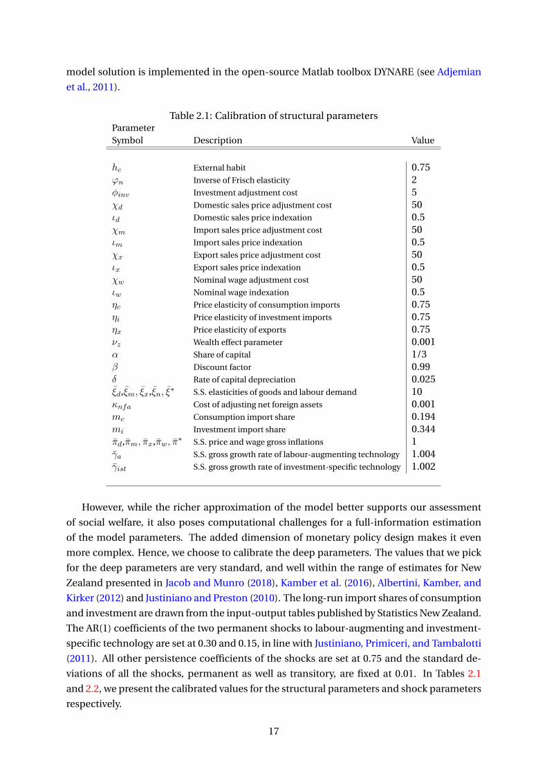
model solution is implemented in the open-source Matlab toolbox DYNARE (see Adjemian
et al., 2011).
Table 2.1: Calibration of structural parametersParameterSymbol Description Value
hc External habit 0.75φn Inverse of Frisch elasticity 2ϕinv Investment adjustment cost 5χd Domestic sales price adjustment cost 50ιd Domestic sales price indexation 0.5χm Import sales price adjustment cost 50ιm Import sales price indexation 0.5χx Export sales price adjustment cost 50ιx Export sales price indexation 0.5χw Nominal wage adjustment cost 50ιw Nominal wage indexation 0.5ηc Price elasticity of consumption imports 0.75ηi Price elasticity of investment imports 0.75ηx Price elasticity of exports 0.75νz Wealth effect parameter 0.001α Share of capital 1/3β Discount factor 0.99δ Rate of capital depreciation 0.025ξd,ξm, ξx,ξn, ξ∗ S.S. elasticities of goods and labour demand 10κnfa Cost of adjusting net foreign assets 0.001mc Consumption import share 0.194mi Investment import share 0.344πd,πm, πx,πw, π∗ S.S. price and wage gross inflations 1γa S.S. gross growth rate of labour-augmenting technology 1.004γist S.S. gross growth rate of investment-specific technology 1.002
However, while the richer approximation of the model better supports our assessment
of social welfare, it also poses computational challenges for a full-information estimation
of the model parameters. The added dimension of monetary policy design makes it even
more complex. Hence, we choose to calibrate the deep parameters. The values that we pick
for the deep parameters are very standard, and well within the range of estimates for New
Zealand presented in Jacob and Munro (2018), Kamber et al. (2016), Albertini, Kamber, and
Kirker (2012) and Justiniano and Preston (2010). The long-run import shares of consumption
and investment are drawn from the input-output tables published by Statistics New Zealand.
The AR(1) coefficients of the two permanent shocks to labour-augmenting and investment-
specific technology are set at 0.30 and 0.15, in line with Justiniano, Primiceri, and Tambalotti
(2011). All other persistence coefficients of the shocks are set at 0.75 and the standard de-
viations of all the shocks, permanent as well as transitory, are fixed at 0.01. In Tables 2.1
and 2.2, we present the calibrated values for the structural parameters and shock parameters
respectively.
17
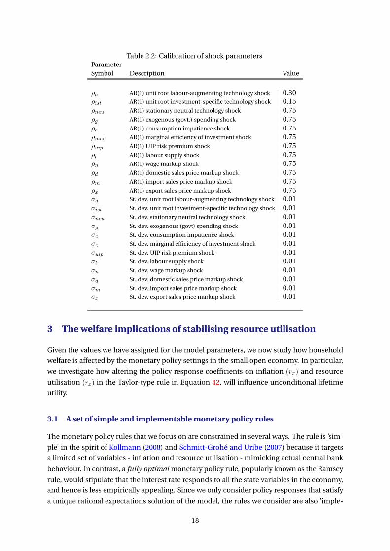
Table 2.2: Calibration of shock parametersParameterSymbol Description Value
ρa AR(1) unit root labour-augmenting technology shock 0.30ρist AR(1) unit root investment-specific technology shock 0.15ρneu AR(1) stationary neutral technology shock 0.75ρg AR(1) exogenous (govt.) spending shock 0.75ρc AR(1) consumption impatience shock 0.75ρmei AR(1) marginal efficiency of investment shock 0.75ρuip AR(1) UIP risk premium shock 0.75ρl AR(1) labour supply shock 0.75ρn AR(1) wage markup shock 0.75ρd AR(1) domestic sales price markup shock 0.75ρm AR(1) import sales price markup shock 0.75ρx AR(1) export sales price markup shock 0.75σa St. dev. unit root labour-augmenting technology shock 0.01σist St. dev. unit root investment-specific technology shock 0.01σneu St. dev. stationary neutral technology shock 0.01σg St. dev. exogenous (govt) spending shock 0.01σc St. dev. consumption impatience shock 0.01σc St. dev. marginal efficiency of investment shock 0.01σuip St. dev. UIP risk premium shock 0.01σl St. dev. labour supply shock 0.01σn St. dev. wage markup shock 0.01σd St. dev. domestic sales price markup shock 0.01σm St. dev. import sales price markup shock 0.01σx St. dev. export sales price markup shock 0.01
3 The welfare implications of stabilising resource utilisation
Given the values we have assigned for the model parameters, we now study how household
welfare is affected by the monetary policy settings in the small open economy. In particular,
we investigate how altering the policy response coefficients on inflation (rπ) and resource
utilisation (rx) in the Taylor-type rule in Equation 42, will influence unconditional lifetime
utility.
3.1 A set of simple and implementable monetary policy rules
The monetary policy rules that we focus on are constrained in several ways. The rule is ’sim-
ple’ in the spirit of Kollmann (2008) and Schmitt-Grohé and Uribe (2007) because it targets
a limited set of variables - inflation and resource utilisation - mimicking actual central bank
behaviour. In contrast, a fully optimal monetary policy rule, popularly known as the Ramsey
rule, would stipulate that the interest rate responds to all the state variables in the economy,
and hence is less empirically appealing. Since we only consider policy responses that satisfy
a unique rational expectations solution of the model, the rules we consider are also ’imple-
18
mentable’ in the terminology used by Schmitt-Grohé and Uribe (2007). To this end, the do-
mains of the optimised policy coefficients for inflation and resource utilisation are restricted
to rπ ∈ [1.01, 2.5] and rx ∈ [0, 2.5] respectively, while the interest rate smoothing coefficient
rr is fixed at 0.5. Since the lower bound on the inflation coefficient exceeds unity, the model
solution is determinate. The domains that we set for the response coefficients subsume the
ranges of estimates presented for several countries in the empirical literature.8 The restricted
grids for the coefficients also aid the numerical searches that we rely on to assess the impact
of monetary policy design on welfare. We experiment with 3 distinct measures of resource
utilisation - the output gap(Y/Y
), the employment gap
(N/N
)and the inverse of the un-
employment rate gap(U/U
). For this reason, the exercise is computationally intensive. The
counterfactual economy that we use as a benchmark to assess the changes in welfare in our
numerical experiments is the version of the model that abstracts from nominal rigidities and
shocks to the price and wage mark-ups (see also Section 2.3.3).
3.2 The welfare metric
The welfare metric that we consider is the ’consumption equivalent variation’ (CEV ), the
constant percentage change that is needed to be made to the representative household’s
consumption in every period and the states of the world so that it is indifferent between
the allocation under a particular policy configuration, i.e. a set of monetary policy response
coefficients, vis à vis the benchmark economy where monetary policy is absent. In other
words, the CEV balances welfare in the counterfactual economy and under the monetary
policy settings that we experiment with.
The traditional CEV involves consumption compensations defined on the consumption
in the current period. The presence of habits in the utility function as in our case (see Equa-
tion 22) complicates the calculation of CEV significantly. In fact, in order to calculate the
traditional CEV in the presence of habits, one has to rely on simulations, and solve for the
CEV using non-linear techniques for every period in the simulations across time horizons.
Indeed, the horizon and the number of simulation periods need to be very large to get reliable
results. Given that we work on large numerical grids of monetary policy response coefficients
in the baseline model as well as many other specifications, this approach quickly becomes
computationally expensive.
A second option to calculate the CEV is to exploit the fact that under all the specifi-
cations we consider, the sticky-price economy, and the benchmark, flexible-price economy,
share the same non-stochastic steady state. In this case, one can compute two auxiliary CEVs
for each economy relative to the non-stochastic steady state. The difference between the two
approximates the CEV between the sticky- and the flexible-price economies remarkably well.
Finally, the CEV can be defined over habit-corrected consumption as in Otrok (2001). We
computed the three variants of the CEV for randomly-selected monetary policy rules, and
8Estimates of the monetary policy response to detrended output in DSGE models are typically very small whilethe estimated responses to inflation are much higher, across countries over time samples. For New Zealand, theaverage estimates are typically between 0.03 and 0.20 (Jacob and Munro, 2018, Kamber et al., 2016, Justinianoand Preston, 2010 and Kam et al., 2009). The estimated inflation coefficients in these studies are usually higher,between 1.9 and 2.33.
19
confirmed that the quantitative differences in results were negligible in our case. The quali-
tative implications for welfare are very similar. For this reason, the rest of this paper focuses
on the habit-corrected measure of the CEV . We will now detail its derivation.
The stationarised form of the utility function is given as
Ut = εct log
(ct − hc
ct−1
γt
)− εctε
lt
zt(ct − hc
ct−1
γt
) n1+φnt
1 + φn, (47)
where the preference shifter is given as zt =(zt−1
γt
)1−vz (ct − hc
ct−1
γt
)vz.9 Defining habit-
corrected consumption as ct = ct − hcct−1
γt, substituting in zt into the utility function and
simplifying,
Ut = εct log ct − εctεlt
(zt−1
γt
)1−vz
cvz−1t
n1+φnt
1 + φn. (48)
Let the expected lifetime utility of the household under the policy settings we want to con-
sider be defined as
Vt ≡ Et
∞∑τ=0
βτ
(εct+τ log ct+τ − εct+τε
lt+τ
(zt+τ−1
γt+τ
)1−vz
cvz−1t+τ
n1+φnt+τ
1 + φn
). (49)
We denote the unconditional lifetime utility of the agent in the counterfactual economy as
VFt . The CEV balances the welfare functions in economies with and without monetary pol-
icy in the following manner:
VFt ≡ Et
∞∑τ=0
βτ
(εct+τ log [(1 + CEV ) ct+τ ]− εct+τε
lt+τ
(zt+τ−1
γt+τ
)1−vz
[(1 + CEV ) ct+τ ]vz−1 n1+φn
t+τ
1 + φn
).
(50)
Expanding the expression on the right hand side,
VFt ≡ Et
∞∑τ=0
βτεct+τ log (1 + CEV ) + Et
∞∑τ=0
βτεct+τ log ct+τ
−Et
∞∑τ=0
βτ
(εct+τε
lt+τ
(zt+τ−1
γt+τ
)1−vz
[(1 + CEV ) ct+τ ]vz−1 n1+φn
t+τ
1 + φn
). (51)
Since Et∑∞
τ=0 εct+τ = 0, this expression reduces to
VFt ≡ log (1 + CEV )
1− β+ Et
∞∑τ=0
βτεct+τ log ct+τ
− (1 + CEV )vz−1Et
∞∑τ=0
βτ
(εct+τε
lt+τ
(zt+τ−1
γt+τ
)1−vz
cvz−1t+τ
n1+φnt+τ
1 + φn
). (52)
9The presence of permanent labour-augmenting and investment-specific technology shocks implies that themodel variables have to be stationarised. Lower case letters are used to represent stationarised variables. SeeJacob and Özbilgin (2021) for more details on stationarisation,
20
Define V1t ≡Et
∑∞τ=0 β
τεct+τ log ct+τand V2t ≡ −Et
∑∞τ=0 β
τεct+τεlt+τ
(zt+τ−1
γt+τ
)1−vzcvz−1t+τ
n1+φnt+τ
1+φn,
so that Vt = V1t + V2
t . In terms of unconditional expectations,
EVFt ≡ log (1 + CEV )
1− β+ EV1
t+(1 + CEV )vz−1 EV2t ,
and the CEV is computed numerically and expressed as a percentage.
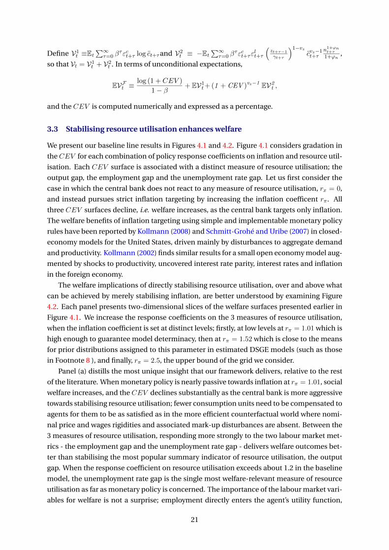
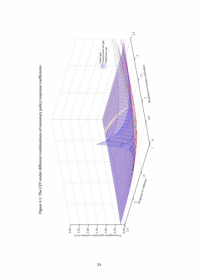
3.3 Stabilising resource utilisation enhances welfare
We present our baseline line results in Figures 4.1 and 4.2. Figure 4.1 considers gradation in
the CEV for each combination of policy response coefficients on inflation and resource util-
isation. Each CEV surface is associated with a distinct measure of resource utilisation; the
output gap, the employment gap and the unemployment rate gap. Let us first consider the
case in which the central bank does not react to any measure of resource utilisation, rx = 0,
and instead pursues strict inflation targeting by increasing the inflation coefficent rπ. All
three CEV surfaces decline, i.e. welfare increases, as the central bank targets only inflation.
The welfare benefits of inflation targeting using simple and implementable monetary policy
rules have been reported by Kollmann (2008) and Schmitt-Grohé and Uribe (2007) in closed-
economy models for the United States, driven mainly by disturbances to aggregate demand
and productivity. Kollmann (2002) finds similar results for a small open economy model aug-
mented by shocks to productivity, uncovered interest rate parity, interest rates and inflation
in the foreign economy.
The welfare implications of directly stabilising resource utilisation, over and above what
can be achieved by merely stabilising inflation, are better understood by examining Figure
4.2. Each panel presents two-dimensional slices of the welfare surfaces presented earlier in
Figure 4.1. We increase the response coefficients on the 3 measures of resource utilisation,
when the inflation coefficient is set at distinct levels; firstly, at low levels at rπ = 1.01 which is
high enough to guarantee model determinacy, then at rπ = 1.52 which is close to the means
for prior distributions assigned to this parameter in estimated DSGE models (such as those
in Footnote 8 ), and finally, rπ = 2.5, the upper bound of the grid we consider.
Panel (a) distills the most unique insight that our framework delivers, relative to the rest
of the literature. When monetary policy is nearly passive towards inflation at rπ = 1.01, social
welfare increases, and the CEV declines substantially as the central bank is more aggressive
towards stabilising resource utilisation; fewer consumption units need to be compensated to
agents for them to be as satisfied as in the more efficient counterfactual world where nomi-
nal price and wages rigidities and associated mark-up disturbances are absent. Between the
3 measures of resource utilisation, responding more strongly to the two labour market met-
rics - the employment gap and the unemployment rate gap - delivers welfare outcomes bet-
ter than stabilising the most popular summary indicator of resource utilisation, the output
gap. When the response coefficient on resource utilisation exceeds about 1.2 in the baseline
model, the unemployment rate gap is the single most welfare-relevant measure of resource
utilisation as far as monetary policy is concerned. The importance of the labour market vari-
ables for welfare is not a surprise; employment directly enters the agent’s utility function,
21
and the stochastic mean and volatility of employment are crucial components of the social
welfare metric. The relevance of the output gap, a combination of the capital stock gap and
the employment gap in our model, is less direct.
Panels (b) and (c) demonstrate that the additional central bank response to resource util-
isation continues to enhance social welfare, even when the inflation coefficient increases.
However, the increases in welfare get progressively milder, and the differences between re-
sponding to different measures of resource utilisation start diminishing already in the more
empirically-relevant case presented in Panel (b), when the inflation coefficient is set at about
1.5. The differences between the CEV curves are almost indistinguishable in Panel (c) when
the inflation coefficient is set at the upper bound of the grid we consider.
The results in Figures 4.1 and 4.2 suggest that the dual mandate works to the benefit of
society. Overall, conditional on all the endogenous frictions and shocks used for our base-
line simulations, it also appears that the dual mandate gives the policy-maker a high degree
of flexibility. When the response to inflation is low, responding more to resource utilisation
yields better welfare outcomes. On the other hand, social welfare also improves even the
central bank pursues strict inflation targeting, disregarding the stabilisation of resource util-
isation. This latter result is reminiscent of the property of ’divine coincidence’ in New Key-
nesian models highlighted by Blanchard and Galí (2007); that monetary policy can stabilise
the welfare-relevant output gap by singularly focussing on stabilising the inflation gap.10 The
difference in our framework is that, within the set of rules we consider, welfare outcomes can
at least improve mildly if the central bank additionally targets resource utilisation. The wel-
fare gains become more substantial, as the central bank places a lower weight on inflation,
and between the various measures of resource utilisation, responding to the labour market
variables appear to be more welfare-enhancing than responding to the output gap. This is
a novel result relative to the extant literature. In the following section, we examine how this
result is strengthened or weakened as we alter the model configuration.
4 Cost-push shocks and the dual mandate
We will now validate the robustness of our baseline results. The first set of checks examine
the implications of changing the strength of the endogenous frictions in the model: (a) full
versus zero indexation in price and wage inflation
(ιd = ιm = ιx = ιw = 1, ιd = ιm = ιx = ιw = 0) (b) remove habit persistence (hc = 0) (c) very
low investment adjustment costs (ϕinv = 0.01) (d) extremely low openness versus much higher
openness (mc = mi = 0.01, mc = mi = 0.50) (e) lower price and wage adjustment costs
(χd = χm = χx = χw = 25) and (f) extreme interest rate inertia (rr = 0.85). The qualitative
insights from the baseline model are preserved in all these model variants; even though the
welfare metrics change in quantitative terms, the analogous profiles of the welfare surfaces
and curves are not dissimilar to those presented in Figures 4.1 and 4.2. The welfare enhance-
ments implied by the dual mandate are apparent in all these reparameterisations.
10The analogue of this property for the open economy has been noted in Corsetti, Dedola, and Leduc (2010).
22
Our model, besides being equipped with the standard set of endogenous frictions, is
driven by a wide array of structural disturbances. Hence, our second set of robustness checks
alter the shock composition. The domestic shocks in the small open economy can be cate-
gorised into three; demand-type disturbances such as those to consumption, investment
and exogenous spending(ϑc, ϑmei, ϑg
), efficient permanent as well as transitory disturbances
on the supply side(ϑa, ϑist, ϑneu, ϑl
)and finally, inefficient cost-push disturbances to price
and wage inflation(ϑpd, ϑpm, ϑpx, ϑn
). The first two categories of shocks are embedded both
in the economy with nominal rigidites and the counterfactual economy without nominal
frictions, while the latter category of inefficient cost-push shocks to the price and wage mark-
ups do not appear in the counterfactual economy. We examine the welfare surfaces gener-
ated when we use the demand-type shocks and efficient supply-type shocks one at a time,
keeping the baseline parameterisation of the endogenous frictions. Again, just as in the case
of the first set of checks that strengthen or weaken the endogenous frictions, the qualitative
insights remain quite similar to the baseline case. The quantitative implications for welfare,
change depending on how strongly the relevant shock influences the business cycle.
The picture changes drastically when we consider the effects of powerful cost-push shocks.
In this final check, we deactivate all other shocks, and empower the inefficient mark-up
shocks to domestic price inflation, imported inflation and wage inflation(ϑpd, ϑpm, ϑn
)by
assigning them 10 times the volatilities used in the baseline model. That is, the standard de-
viations of these shocks are set as σd = σm = σn = 0.1 as opposed to σd = σm = σn = 0.01 in
the baseline. However, the persistence coefficients retain the same values as in the baseline:
ρd = ρm = ρn = 0.75. We present the associate welfare (CEV ) surfaces in Figure 4.3. Since we
earlier saw that the welfare implications of responding to resource utilisation are most ob-
vious when the inflation response coefficient is very low (rπ = 1.01), we present this special
case in Figure 4.4.
Figure 4.3 establishes that, in the presence of powerful cost-push shocks to price and
wage inflation, welfare decreases (CEV increases) as the central bank reacts more to re-
source utilisation. This is the opposite pattern relative to that seen in our baseline specifica-
tion, and is observed for all levels of inflation stabilisation. Furthermore, we also observe in
Figure 4.4, that among the 3 measures of resource utilisation we experiment with, responding
to the output gap delivers worse welfare outcomes than reacting to the labour market vari-
ables. A crucial determinant of the welfare implications of price and wage mark-up shocks, is
the fact that they drive inflation and resource utilisation in opposite directions. When these
shocks exert powerful influences on the business cycle, the central bank faces trade-offs be-
tween the dual objectives of stabilising inflation and stabilising resource utilisation. This is
in contrast to the disturbances to aggregate demand or technical progress.11 Finally, revert-
ing back to Figure 4.3, we find that, in the face of powerful cost-push shocks, society is better
served when the central bank focusses solely on stabilising inflation, ignoring the resource
utilisation objective.
11Mankiw (2007) provides an intuitive account of the implications of demand shocks, productivity shocks, andcost-push shocks for the covariance between inflation and the output gap, and hence for monetary polcy trade-offs.
23
Figu
r e4.
1:T
he
CE
Vu
nd
erd
iffe
ren
tco
mb
inat
ion
so
fmo
net
ary
po
licy
resp
on
seco
effi
cien
ts
24
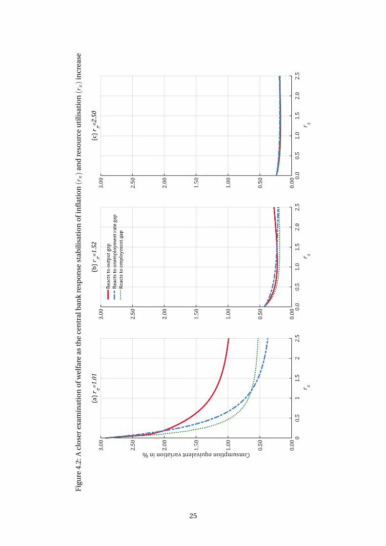
Figu
r e4.
2:A
clo
ser
exam
inat
ion
ofw
elfa
reas
the
cen
tral
ban
kre
spo
nse
stab
ilisa
tio
no
fin
flat
ion(r
π)
and
reso
urc
eu
tili
sati
on(r
x)
incr
ease
25
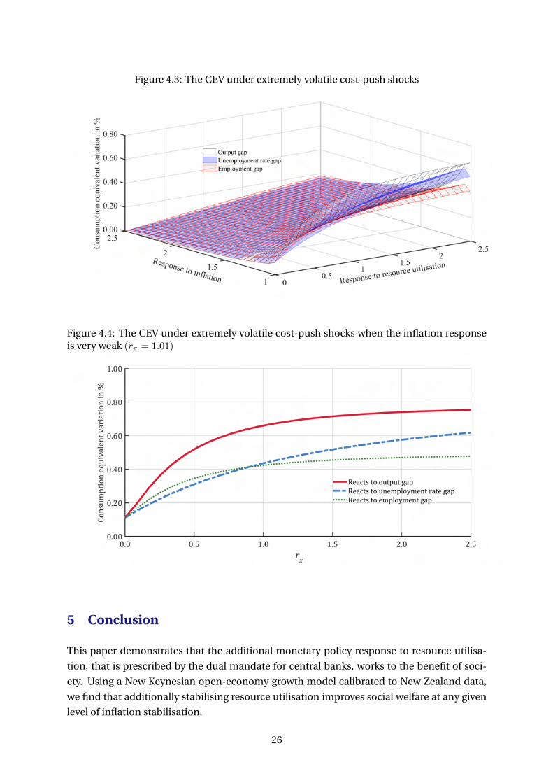
Figure 4.3: The CEV under extremely volatile cost-push shocks
Figure 4.4: The CEV under extremely volatile cost-push shocks when the inflation responseis very weak (rπ = 1.01)
5 Conclusion
This paper demonstrates that the additional monetary policy response to resource utilisa-
tion, that is prescribed by the dual mandate for central banks, works to the benefit of soci-
ety. Using a New Keynesian open-economy growth model calibrated to New Zealand data,
we find that additionally stabilising resource utilisation improves social welfare at any given
level of inflation stabilisation.
26
The welfare gains from stabilising resource utilisation are particularly striking when the
central bank is nearly passive towards stabilising inflation response to inflation is weak. In-
terestingly, when the sensitivity to inflation is weak, monetary policy responses to the labour
market variables such as the employment gap or the unemployment rate gap, that are more
in line with the activity indicators stipulated in actual central bank legislation, yield better
welfare outcomes than reacting to the most popular summary indicator of resource utilisa-
tion: the output gap. This is mainly because the levels and volatilities of employment and
consumption are crucial components of the social welfare metric that underpins modern
normative macroeconomics. The implications of stabilising the output gap, that is also in-
fluenced by several other elements in general equilibrium, are less direct as far as the welfare
metric is concerned.
However, within the range of monetary policy settings we consider, the welfare gains from
stabilising resource utilisation decline to mild levels when the central bank is already very
sensitive to inflation. Not surprisingly, in this scenario, the differences between the welfare
implications of stabilising the three different measures of resource utilisation also diminish.
The overall desirability of stabilising resource utilisation from the perspective of social
welfare is robust across several variants of our theoretical framework. However, the challenge
that the monetary policy-maker confronts is also an empirical one; the clouds of uncertainty
that shroud assessments of the level of resource utilisation in the economy. Data series such
as those for GDP and the unemployment rate are occasionally subject to revisions by sta-
tistical agencies, and the econometric measurement of the activity gap is also known to be
complex (Orphanides and van Norden, 2002). From this practical viewpoint, the dual man-
date is also the more difficult mandate for the policy-maker. Inflation targeting is a simpler
framework, and since the policy response to inflation can deliver welfare outcomes almost
as high as those generated by the response to resource utilisation in our model, we conclude
that inflation targeting remains an appealing alternative monetary policy framework.
References
Adjemian, S., Bastani, H., Karamé, F., Juillard, M., Maih, J., Mihoubi, F., Perendia, G., Pfeifer, J.,
Ratto, M., Villemot, S., 2011. Dynare: Reference Manual Version 4. Dynare working papers,
CEPREMAP.
Adolfson, M., Laséen, S., Lindé, J., Svensson, L., 2014. Monetary policy trade-offs in an es-
timated open-economy DSGE model. Journal of Economic Dynamics and Control 42 (C),
33–49.
Adolfson, M., Laséen, S., Lindé, J., Villani, M., 2007. Bayesian estimation of an open-economy
DSGE model with incomplete pass-through. Journal of International Economics 72 (2),
481–511.
Albertini, J., Kamber, G., Kirker, M., 2012. An estimated small open economy model with
frictional unemployment. Pacific Economic Review 17 (2), 326–353.
27
Andreasen, M. M., 2012. An estimated DSGE model: Explaining variation in nominal term
premia, real term premia, and inflation risk premia. European Economic Review 56 (8),
1656–1674.
Blanchard, O., Galí, J., 2007. Real wage rigidities and the New Keynesian model. Journal of
Money, Credit and Banking 39 (s1), 35–65.
Bodenstein, M., Kamber, G., Thoenissen, C., 2018. Commodity prices and labour market dy-
namics in small open economies. Journal of International Economics 115 (C), 170–184.
Calvo, G. A., 1983. Staggered prices in a utility-maximizing framework. Journal of Monetary
Economics 12 (3), 383–398.
Christiano, L., Trabandt, M., Walentin, K., 2011. Introducing financial frictions and unem-
ployment into a small open economy model. Journal of Economic Dynamics and Control
35 (12), 1999–2041.
Corbo, V., Strid, I., 2020. MAJA: A two-region DSGE model for Sweden and its main trading
partners. Working Paper Series 391, Sveriges Riksbank.
Corsetti, G., Dedola, L., Leduc, S., 2010. Optimal monetary policy in open economies. In:
Friedman, B. M., Woodford, M. (Eds.), Handbook of Monetary Economics. Vol. 3 of Hand-
book of Monetary Economics. Elsevier, Ch. 16, pp. 861–933.
Corsetti, G., Dedola, L., Leduc, S., 2020. Exchange rate misalignment and external imbal-
ances: What is the optimal monetary policy response? Working Paper Series 2020-04, Fed-
eral Reserve Bank of San Francisco.
De Paoli, B., 2009. Monetary policy and welfare in a small open economy. Journal of Interna-
tional Economics 77 (1), 11–22.
Debortoli, D., Kim, J., Lindé, J., Nunes, R., 2019. Designing a simple loss function for central
banks: Does a dual mandate make sense? Economic Journal 129 (621), 2010–2038.
Erceg, C., Henderson, D., Levin, A., 2000. Optimal monetary policy with staggered wage and
price contracts. Journal of Monetary Economics 46 (2), 281–313.
Fujiwara, I., Wang, J., 2017. Optimal monetary policy in open economies revisited. Journal of
International Economics 108 (C), 300–314.
Galí, J., 2011. The return of the wage Phillips Curve. Journal of the European Economic Asso-
ciation 9 (3), 436–461.
Galí, J., Smets, F., Wouters, R., 2012. Unemployment in an estimated New Keynesian model.
NBER Macroeconomics Annual 26 (1), 329–360.
Ilbas, P., 2012. Revealing the preferences of the US Federal Reserve. Journal of Applied Econo-
metrics 27 (3), 440–473.
28
Jacob, P., Munro, A., 2018. A prudential stable funding requirement and monetary policy in a
small open economy. Journal of Banking and Finance 94 (C), 89–106.
Jacob, P., Özbilgin, M., 2021. Not-for-publication technical appendix to Welfare gains in a
small open economy with a dual mandate for monetary policy. Available on request.
Justiniano, A., Preston, B., 2010. Monetary policy and uncertainty in an empirical small open-
economy model. Journal of Applied Econometrics 25 (1), 93–128.
Justiniano, A., Primiceri, G., Tambalotti, A., 2011. Investment shocks and the relative price of
investment. Review of Economic Dynamics 14 (1), 101–121.
Kam, T., Lees, K., Liu, P., 2009. Uncovering the hit list for small inflation targeters: A Bayesian
structural analysis. Journal of Money, Credit and Banking 41 (4), 583–618.
Kamber, G., McDonald, C., Sander, N., Theodoridis, K., 2016. Modelling the business cycle
of a small open economy: The Reserve Bank of New Zealand’s DSGE model. Economic
Modelling 59 (C), 546–569.
Kollmann, R., 2002. Monetary policy rules in the open economy: Effects on welfare and busi-
ness cycles. Journal of Monetary Economics 49 (5), 989–1015.
Kollmann, R., 2008. Welfare-maximizing operational monetary and tax policy rules. Macroe-
conomic Dynamics 12 (S1), 112–125.
Mandelman, F., Rabanal, P., Rubio-Ramirez, J. F., Vilán, D., 2011. Investment-specific tech-
nology shocks and international business cycles: An empirical assessment. Review of Eco-
nomic Dynamics 14 (1), 136–155.
Mankiw, N. G., 2007. Comments presented at Federal Reserve Conference; Price dynamics:
Three open questions. Journal of Money, Credit and Banking 39 (s1), 187–192.
Mortensen, D., Pissarides, C., 1994. Job creation and job destruction in the theory of unem-
ployment. Review of Economic Studies 61 (3), 397–415.
Orphanides, A., van Norden, S., 2002. The unreliability of output-gap estimates in real time.
The Review of Economics and Statistics 84 (4), 569–583.
Otrok, C., 2001. On measuring the welfare cost of business cycles. Journal of Monetary Eco-
nomics 47 (1), 61–92.
RBNZ, 2019. The remit for the Monetary Policy Committee. https://www.rbnz.govt.nz/
monetary-policy/about-monetary-policy/monetary-policy-framework.
Reserve Bank of Australia, 2020. Annual report. https://www.rba.gov.au/publications/
annual-reports/rba/2020/pdf/2020-report.pdf.
Rotemberg, J., 1982. Monopolistic price adjustment and aggregate output. Review of Eco-
nomic Studies 49 (4), 517–31.
29
Schmitt-Grohé, S., Uribe, M., 2003. Closing small open economy models. Journal of Interna-
tional Economics 61 (1), 163–185.
Schmitt-Grohé, S., Uribe, M., 2007. Optimal simple and implementable monetary and fiscal
rules. Journal of Monetary Economics 54 (6), 1702–1725.
Smets, F., Wouters, R., 2007. Shocks and frictions in US business cycles: A Bayesian DSGE
approach. American Economic Review 97 (3), 586–606.
Steelman, A., 2011. The Federal Reserve’s dual mandate: The evolution of an idea. Richmond
Fed Economic Brief (Dec).
Svensson, L. E., 2014. How to weigh unemployment relative to inflation in monetary policy?
Journal of Money, Credit and Banking 46 (S2), 183–188.
A Appendix
30
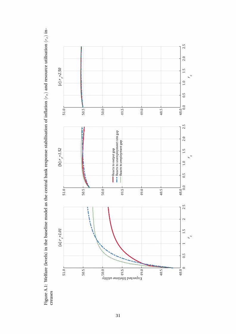
Figu
reA
.1:
Wel
fare
(lev
els)
inth
eb
asel
ine
mo
del
asth
ece
ntr
alb
ank
resp
on
sest
abili
sati
on
of
infl
atio
n(r
π)
and
reso
urc
eu
tili
sati
on(r
x)
in-
crea
ses
31