on the automatic recovery of style-speciﬁc …spiros/papers/ause02.pdfp1: dhirendra samal (gje)...

P1: Dhirendra Samal (GJE)

Automated Software Engineering KL1496-01 July 30, 2002 14:2

Automated Software Engineering, 9, 331–360, 2002c© 2002 Kluwer Academic Publishers. Manufactured in The Netherlands.

On the Automatic Recovery of Style-SpecificArchitectural Relations in Software Systems

MARTIN TRAVERSO [email protected] MANCORIDIS [email protected] of Mathematics and Computer Science, Drexel University, Philadelphia, PA, USA

Abstract. The cost of maintaining a software system over a long period of time far exceeds its initial developmentcost. Much of the maintenance cost is attributed to the time required by new developers to understand legacysystems. High-level structural information helps maintainers navigate through the numerous low-level componentsand relations present in the source code. Modularization tools can be used to produce subsystem decompositionsfrom the source code but do not typically produce high-level architectural relations between the newly foundsubsystems. Controlling subsystem interactions is one important way in which the overall complexity of softwaremaintenance can be reduced.

We have developed a tool, called ARIS (Architecture Relation Inference System), that enables software en-gineers to define rules and relations for regulating subsystem interactions. These rules and relations are calledInterconnection Styles and are defined using a visual notation. The style definition is used by our tool to infersubsystem-level relations in designs being reverse engineered from source code.

In this paper we describe our tool and its underlying techniques and algorithms. Using a case study, we describehow ARIS is used to reverse engineer high-level structural information from a real application.

Keywords: reverse engineering, software maintenance, software architecture

1. Introduction

As source code is often the only up-to-date specification available to software developers, asignificant body of research in reverse engineering is devoted to techniques for recoveringhigh-level structural information from source code (Chikofsky and Cross, 1990). Thesetechniques rely on first gathering information about the source code components (e.g., pro-cedures, classes) and relations between these components (e.g., procedure invocation, classinheritance) using tools (Krishnamurthy, 1995; Chen et al., 1997) for source code analysis.

Using component and relation information derived from the source code analysis process,along with other information obtained from designers and documentation (Biggerstaff,1989), components of the system are clustered (grouped) (Schwanke, 1991; Muller et al.,1992; Tzerpos and Holt, 1998; Mancoridis et al., 1998) into composite components, calledsubsystems. Subsystems are, in turn, recursively clustered into higher-level subsystems,and so on. The clustering is not done arbitrarily. Rather, components are clustered usingcommon-sense principles, such as cohesion and coupling. The cohesion principle states thatclustered components should exhibit a high degree of interrelation. The coupling principlestates that inter-cluster relations should be kept to a minimum. Other criteria for clusteringmay also be used. For example, one may use domain concepts to cluster components, orone may group components that are likely to change at the same time.



332 TRAVERSO AND MANCORIDIS

It is clear that modularization techniques help designers produce subsystem decompo-sitions. This is a useful starting point in the software maintenance process. Our researchcomplements existing reverse engineering techniques by providing algorithms for com-puting the interfaces and relations between the subsystems that are created during thereverse engineering process. Unlike a typical procedural interface—which is composed ofa set of variables—or a typical module or class interface—which is composed of a setof procedures—a subsystem interface is composed of a set of modules, classes, or othersubsystems. Hence, just as exported (visible) procedures comprise the interface of modulesand classes, the interface of subsystems typically consist of exported modules, classes, andother subsystems.

We have developed a tool, called ARIS (Architecture Relation Inference System), thatenables software developers to provide descriptions of rules and relations to regulate howmodules and subsystems can relate to each other. We call these descriptions interconnec-tion styles. The relations are abstract (high-level) and cannot be found directly in either thesource code or the subsystem hierarchy of the software. Interconnection styles allow de-signers to control the interactions between components by use of rules and subsystem-levelrelations. When the relations are not present in the recovered subsystem decomposition,ARIS automatically infers the relations that are missing in order for the design to satisfythe restrictions imposed by the interconnection style. ARIS is also able to validate whethera design that already contains high-level relations satisfies a set of constraints imposed bythe style (i.e., stylistic constraints).

Next, we define the term interconnection style and provide an example of a design thatfollows a specific style description.

1.1. Example of a design following a style description

We define an interconnection style to be a description of:

1. the types of components in the design (e.g., module, subsystem)2. the types of relations in the design (e.g., import, export)3. the set of all well-formed (syntactically legal) configurations of components and relations4. the semantics of each well-formed configuration (e.g., exported components are visible

to external client components)

The Export style facilitates the specification of subsystem interfaces. Subsystem inter-faces are defined using the export relation between two components. For example, if asubsystem S exports a module M , the module is considered part of the interface of S. Notethat the export relations would not be produced by existing modularization (clustering)techniques. This is not surprising, since the export relation is not found in the source code.

ARIS defines relations that are part of the style being followed by a design. We callsuch relations style-specific relations. The user specifies the stylistic constraints visuallyand ARIS uses this description to induce the missing relations automatically. ARIS isalso capable of validating a design that contains high-level structural relations against aninterconnection style. The syntax for style specifications is based on the Interconnection



AUTOMATIC RECOVERY OF STYLE-SPECIFIC ARCHITECTURAL RELATIONS 333

Figure 1. Recovering a software design that follows the export style.

Style Formalism (ISF) (Mancoridis, 1997, 1998). A detailed example of an ISF specification,which is based on GraphLog (Consens and Mendelzon, 1990) is given in Section 1.2.

The top of figure 1 presents the source-level modules (depicted as rectangles) of a softwaresystem. Edges represent binary relations, such as uses relations between modules. Hence,module M4 uses module M5 means that procedures in M4 call procedures or referencevariables and types in M5. The diagram is an example of a Module Dependency Graph(MDG). An MDG is a set of nodes connected by directed edges. Nodes represent source-levelcomponents of a software systems, while edges represent source-level relations betweenthe components. The middle of the same figure shows a clustering of the system into asubsystem hierarchy. White rectangles depict subsystems. The nesting of rectangles is thecontainment relation. To make this design follow the Export style, ARIS must induce themissing export relations. The bottom of figure 1 shows these missing relations.




In the Export style, the use relations between modules are controlled by encapsulatingmodules into subsystems with well-defined interfaces. An encapsulated module may be usedby other modules outside of its parent subsystem (container) if the encapsulated moduleis exported by its parent. For example, in subsystem SS3, module M6 is allowed to usemodule M4 because the latter is part of the interface of the subsystem containing it, namelySS4. Furthermore, the relation between module M1 and M4 is permitted because M4 istransitively exported from subsystem SS3 (M4 is exported from SS4 and SS4 is, in turn,exported from SS3).

However, module M6 is not permitted to use module M5, because the latter is not exportedfrom (i.e., is not part of the interface of) SS4. If M6 were modified to use M5, our designwould have a stylistic violation. Such violations may guide designers, during the softwaremaintenance phase, to take one of three actions:

1. remove the relation that causes the violation2. add missing subsystem relations to make the design well-formed (e.g., specify that SS4

exports M5)3. re-modularize the design to make it well-formed (e.g., move M5 from SS4 to SS3)

Interconnection styles also provide context within which to perform various kinds ofanalyses on software designs. For example, we can define a measurement for subsysteminterface complexity to help identify subsystems that export an extraordinarily high per-centage of their contained components. A measurement such as interface complexity couldprovide guidance in the evolution of the structure of a system.

Before outlining our work we provide an example of style specification using ISF.

1.2. ISF specification of the export style

ISF is a visual notation that enables designers to specify constraints on configurationsof components and relations, and the semantics of such configurations. Circles representsystem components (e.g., modules, subsystems) and arrows represent relations betweencomponents (e.g., import, export, use).

This notation depicts rules as directed labeled graphs, allowing all relations, including thecontainment relation to be represented uniformly as directed edges. The nodes in the graphrepresent modules and subsystems. Note that the containment relation is not represented asnested boxes as in figure 1, but as a simple labeled edge. Figure 2 depicts an example of aset of style constraints defined using the ISF notation.

In the Export style, use relations between modules are controlled by encapsulating mod-ules into subsystems with well-defined interfaces. An encapsulated module may be usedby other modules outside of its parent subsystem (container) if the encapsulated moduleis exported by its parent. These constraints are described by the graphs in figure 2. Eachrule is represented by a distinct graph, and each graph contains a single dashed arrow. Themeaning of the dashed arrow depends on the kind of rule.

There are two kinds of rules:

1. Permission rules, labeled PERMIT, define the set of well-formed configurations of soft-ware designs that follow a specific style.




Figure 2. ISF specification of the export style.

2. Definition rules, labeled DEFINE, are used to define new relations based on patterns ofcomponents and relations.

The meaning of each of the three rules that comprise the ISF specification of figure 2 isgiven below. We provide both an informal English description and a formal predicate logicdescription.

– PERMIT(1)

• Informal: A subsystem may be exported by the subsystem that contains it. The dashedarrow represents the permitted export relation. Only subsystems contained in othersubsystems are allowed to export their children (i.e., subsystems may not be exportedoutside the application, represented by the root subsystem).

• Formal: ∀ SS0, SS1, SS2 ((contains(SS0, SS1) ∧ contains(SS1, SS2)) ⇒ can export(SS1, SS2))

– PERMIT(2)

• Informal: A subsystem or module SS1 can use another subsystem or module SS2 ifSS1 sees SS2.

• Formal: ∀ SS1, SS2 (sees(SS1, SS2) ⇒ can use(SS1, SS2))

– DEFINE(1)

• Informal: A module SS1 can see another module SS2 if SS2 is transitively exported toa common level with an ancestor of SS1. Unlike permission rules, which specify whendesign relations are permitted to occur, definition rules actually define new relations(e.g., relation see).

• Formal: ∀ PP, PSS1, PSS2, SS1, SS2 ((contains(PP, PSS2) ∧ contains(PP, PSS1) ∧transitive contains(PSS1, SS1) ∧ transitive contains(PSS2, SS2) ∧ transitive exports(PSS2, SS2) ∧ PSS1 �= PSS2) ⇒ sees(SS1, SS2))




In this section we introduced ARIS and briefly explained its role in forward and reverseengineering. We then defined interconnection styles and showed an example of a designthat follows the Export Style.

Next, we describe ARIS in more detail and provide a short example to demonstrate how itcan be integrated with existing reverse-engineering tools. Then, we proceed to describe thetechniques and algorithms underlying ARIS and, finally, we present a case study showinghow it can be used to analyze a real-world application.

2. ARIS (architecture relation inference system)

ARIS has two main components, namely, the Style Editor and the Edge Repair Utility.The Style Editor allows the user to define style specifications visually using simple graphicelements, such as circles and arrows, as shown in figure 2. The Edge Repair Utility performsthe well-formedness validation of a design and the automatic induction of missing relationswith respect to a style.

2.1. Style editor

Figure 3 shows the main screen of the Editor. The toolbar initially contains the node tooland three built-in edge tools, namely, contain, see, and not equal. The user can create toolsfor additional relation types, such as the export relation shown in figure 3. The color andlabel of a relation type, with the exception of built-in relations, can be modified by the user.

Figure 3. Defining the export style using the style editor.




Permission and definition rules are created through the appropriate menu commands.Rules are drawn by placing nodes into the rule window and connecting them with relationedges. Rules are required to have exactly one target relation (i.e., the relation that is beingpermitted or defined).

Style descriptions must provide at least one definition for the see relation. The permissionrule for the use relation is also mandatory. Informally, the permission rule states that a useedge between two modules SS1 and SS2 is allowed if module SS1 sees module SS2.Formally, can use(SS1, SS2) ⇔ see(SS1, SS2). This rule is common to every style and,thus, ARIS assumes it implicitly.

2.2. Edge repair utility

The modules and relations of a system are mapped to a Module Dependency Graph (MDG).The nodes in an MDG correspond to the modules of the system and the edges representsource-level relations (e.g., procedural invocation). The MDG can be constructed automati-cally using readily available source code analysis tools, such as CIA (Krishnamurthy, 1995)for C, Acacia (Chen et al., 1997) for C and C++, and Chava (Korn et al., 1999) for Java.Modules can be mapped to different language constructs, depending on the desired levelof granularity of the analysis. For example, in C, a module could be mapped to a source orheader file, or to a set of files whose name begins with a certain keyword that indicates thatthe files are part of the same logical module. On the other hand, in languages such as C++and Java, a module could be mapped to a class, and relations would include method calls,class inheritance, et cetera. An example of an MDG is shown in figure 4. This MDG showsthe modules and relations of Mini Tunis, an experimental operating system used for teachingwritten in the object-oriented Turing language. Modules in Mini Tunis’ MDG correspondto Turing modules in the source code. The MDG can be clustered into subsystems by toolssuch as Bunch (Mancoridis et al., 1999). Figure 5 shows the result of clustering the MiniTunis MDG. Subsystems are groupings of modules and smaller subsystems.

ARIS takes a clustered MDG as input and attempts to find the missing style relations.Hence, it assumes that the first two steps of the reverse-engineering process (i.e., sourcecode analysis and software clustering) have taken place.

The goal is to induce a set of style relations that will make all of the use relations well-formed. A relation is well-formed if it does not violate any permission rule described bythe style. A solution to this problem, which we call the edge repair problem, not only hasto be well-formed, but it must limit the exposure (visibility) of encapsulated modules andsubsystems as much as possible, which is a desirable property of good designs. Visibilityis a measure of the degree of subsystem exposure or, more concretely, of the number of seerelations that can be induced in a design.

Figure 6 shows how our Style Editor and Edge Repair tools can be integrated with sourcecode analysis tools and the Bunch clustering tool. The Edge Repair Utility accepts twoinputs, namely, the MDG and Cluster Tree specifications as well as the style definition.Relations in the style definition are classified into two categories: use and style. The userelations include all source-level relations, whereas the style relations include all style-specific relations. The Edge Repair Utility algorithm finishes either when every relation is




Figure 4. The module dependency graph (MDG) of mini tunis.

well-formed or when no more relations can be made well-formed. The first case impliesthat a solution was found; the second case, that there is no way to make every use relationwell-formed.

Results are displayed using dotty, a graph visualization tool (Gansner et al., 1993).Figure 7 shows the result of finding the missing relations for Mini Tunis (figure 5) withrespect to the Export style (figure 2). For clarity, use relations are not shown in the diagram.Subsystems are represented by nodes, unlike the diagram in figure 5 which represents themas nested boxes. The containment relations are drawn as thin arrows, while thick arrowsrepresent the induced export relations. For example, in figure 7, subsystem 20 containssubsystem 18, which in turn contains subsystem 13, which in turn contains modules Inodeand Device. Note that subsystem 18 exports subsystem 13, which in turn exports both Inodeand Device. Subsystems contained by subsystem 17 are not exported, so they mostly behaveas clients for the modules contained in subsystems 18 and 19 that are exported. Subsystem16 does not export any of its modules, so it behaves as a client (i.e., its modules use othermodules but are not used by any modules). Modules in subsystems 1 and 10 are exported,




Figure 5. The automatically produced MDG clustering of mini tunis.

Figure 6. Integration of reverse engineering tools.




Figure 7. The result of repairing mini tunis’ design.

meaning that they are used by modules outside of 1 or 10, respectively. These subsystemsbehave as suppliers for modules contained in subsystem 17.

When the input MDG already contains style relations the Edge Repair Utility can be usedto check whether the design is well-formed. ARIS reports the number of relations that arewell-formed or ill-formed and highlights those that are ill-formed in the diagram.

3. Techniques

We have presented a tool that can be used to find the missing style relations in a designwith respect to a style definition. In this section we describe the algorithms and techniquesbehind it.

An exhaustive approach to solving the edge repair problem is to try all possible config-urations of relations permitted by the style and keep track of the one that satisfies all of theconstraints of the style and minimizes overall exposure of modules. While this approach




might work for small systems, using it on larger systems is not feasible since the numberof possible configurations grows exponentially with respect to the size of the system.

To understand why, let us consider a graph with N nodes. The maximum number of edgesthat can exist in the graph for each permitted relation type (e.g., export, import) is E = N 2

(i.e., one edge coming out of each node and into every other node, as well as the sourcenode itself). If the style permits R different relation types, the graph can contain a total ofM = RE = RN 2 style relations. What we need to know, however, is how many possiblesolutions exist to the edge repair problem. There are ( M

0 ) = 1 possible configurations thatcontain 0 edge, ( M

1 ) = M configurations that contain 1 edge, ( M2 ) = M(M−1)

2 configurationsthat contain 2 edges, and so on. The total number of configurations, thus, is given by thefollowing expression:

M∑e=0

(M

c

)= 2M = 2RN2

Even for a small graph, such as the one shown in figure 8, the number of possibleconfigurations is large. A graph with 8 nodes (i.e., E = 82 = 64) would yield 264 possibleconfigurations for a style that permits only one relation (e.g., the Export Style depicted infigure 2).

A slightly better approach would avoid considering relations that can never be well-formed when enumerating the possible configurations. For example, the permission rulesof the Export style do not allow a module to export itself, or a child module to export itsparent subsystem. The number of permissible edges in figure 8 for the Export style is nowreduced to 5 (i.e., only the export relations 1-A, 1-B, 2-C, 2-D and 2-E are allowed by thestyle). The number of possible configurations is now 25 = 32. Although it would be feasibleto generate all possible configurations for such a small system, there is still an exponentialrelation between the number of nodes and the total number of configurations, making theproblem intractable for large systems. Moreover, in the worst case, the style might allowrelations to occur between any pair of modules and we would fall back to the brute forcescenario described previously.

It is clear that neither approach works, so other ways of solving the problem must beexplored. In the next section we explain how the edge repair problem can be treated as anoptimization problem and we describe some techniques that can be used to find good (ifnot optimal) solutions.

Figure 8. Example of a small structure graph with no style relations.




3.1. Edge repair as an optimization problem

Many problems have more than one possible solution and sometimes, even hundreds orthousands of them. Almost always, solutions can be ranked according to their desirability,so finding an arbitrary solution is usually not enough, and a good solution (if not the bestone) is really needed. Problems of this kind are referred to as optimization problems. Thequality of a solution is usually characterized by a mathematical function that quantifiesquality is usually referred to as the objective function or fitness function, and is the core ofany optimization problem.

It is clear that visibility must be factored into our fitness function (i.e., we are tryingto minimize visibility). Visibility measures the extent of exposure of the components of asystem to the rest of the components in the same system. We are still left with the problemof finding a well-formed configuration, however. Generating and testing all possible config-urations is out of the question, but nicely enough, well-formedness can also be incorporatedinto the scheme. We can measure the well-formedness of a configuration in terms of thenumber of well-formed and ill-formed relations it contains. Given these premises, we candefine our new goal as finding a configuration that makes every use edge well-formed whilekeeping the number of ill-formed relations and visibility low. Thus, the quality measurementshould exhibit the following properties:

– configurations with a large number of well-formed use relations should get a high qualityscore

– configurations with a large number of ill-formed style relations should get a low qualityscore

– configurations with large visibility (i.e., many see relations) should get a low qualityscore

Before describing the optimization techniques we digress in Sections 3.2 and 3.3 toanalyze some issues related to the quantification of visibility and the search process.

3.2. Measuring visibility

Visibility is a measure of the number of see edges that can be induced from a configuration ofstyle relations. A naıve approach for measuring visibility would involve testing if visibility(see) relations can be induced for each pair of nodes in the graph, which is clearly an O(N 2)operation. As we will see in Section 3.8, each test can be quite expensive, especially forcomplex rules. Moreover, since visibility needs to be computed frequently (see Section 3.5),a cheaper method for computing it is needed.

We identified three ways of computing visibility. Unlike the first two methods, whichcompute visibility by operating on the structure of the system and rule definitions, the thirdmethod makes a simplifying assumption to reduce the complexity of the operation. Thethree methods are outlined below.

1. Induction. See relations are induced from the configurations of style relations by match-ing style rules to the structure of the system. The difficulty of this method resides in the




fact that all matches must be found, which cannot be done easily without testing everypair of nodes (i.e., we fall into the brute force).

2. Incremental update. Starting from an initial configuration whose visibility is known(i.e., it is pre-computed during initialization time, probably using an induction or a bruteforce method), visibility is updated incrementally by analyzing the effects of adding orremoving style relations to the previous configuration. The lack of locality of effectsdue to addition and removal of edges can escalate the complexity of such an operation.For example, adding an export relation between a subsystem A and one of its children,B, can cause all of B’s children, which might have been exported, to become visibleoutside of A’s subtree. This inherent complexity is worsened by the fact that findingwhich see relations are affected by the addition or removal of style relations can be veryhard. This method could, however, provide some performance enhancement over the firstapproach.

3. Simplistic visibility. Many styles display a correlation between the number of stylerelations and visibility. This derives from the fact that the rules that can be described usingISF are “constructive”, meaning that they allow relations to exist but do not disallowthem explicitly (i.e., negated relations are not permitted by the notation). Therefore,adding style relations to a given configuration can only increase its overall visibility. Asimplistic measure of visibility could then be defined in terms of the number of stylerelations contained by a configuration.

It is tempting to use the simplistic visibility measure for our problem, since it reduces thecomplexity of the computation from O(N 2) to O(1). There is a caveat, however. Simplisticvisibility is based on the assumption that fewer style relations imply a solution with lessvisibility. However, this is not always the case. Consider the style defined in figure 9, whichallows a module to be seen by another module whenever it is imported directly, or when itsparent is imported. The result of inducing the missing style relations for the system depictedin figure 8 using standard visibility is shown in figure 10(a). Similarly, figure 10(b) showsthe result when simplistic visibility is used. Overall visibility in result 10(a) is 4 (A see D,A see E, B see D, B see E), whereas 10(b) has a visibility of 8 (A see D, A see E, A see C,A see 2, B see D, B see E, B see C, B see 2), but 10(a) contains more style relations than10(b). This example is a special case of a wider range of styles that violate the simplisticvisibility assumption. We have not been able to characterize these styles formally, but someof their properties are listed below.

Figure 9. Style for which the simplistic visibility assumption does not hold.




Figure 10. Results obtained after repairing a design using different visibility measurements.

Figure 11. Examples of rules that violate the simplistic visibility assumption.

– The style is non-recursive. Permission rules are not defined in terms of other permissionrules, allowing relations to occur at lower levels of the tree without getting permissionfrom higher-level relations.

– A module can be exposed by a relation connected to it or any of its ancestors, with noother restriction.

Other examples of rules belonging to styles that violate the simplistic visibility assumptionare shown in figure 11. Note that these rules can expose entire subtrees by adding a singlerelation.

We have come to a point where we need to decide whether to use the standard or thesimplistic visibility measure. Clearly, there is a trade-off between generality and complexity.The tests we performed showed that computing traditional visibility is too expensive and, onthe other hand, simplistic visibility works for a large percentage of commonly used styles. Wedecided to sacrifice the ability to handle a small percentage of styles correctly for a decreasein complexity. In fact, most styles that do not work well with simplistic visibility are usuallyexamples of poorly designed styles. Take, for example, a specification that regulates theinteractions for a programming language. A style that allows entire containment subtrees tobe exposed with the addition of a single style relation is analogous to a language that allowsclasses or modules, along with all their private and public methods, instance variables andeven local variables to be exposed by a single language construct. This is clearly not adesirable feature of a programming language.

3.3. Pessimistic edge reparability

We have already analyzed the complexity of the brute force approach to finding the missingstyle relations. We briefly described a trivial optimization that could reduce its complexity




by a large factor. In particular, we saw how the missing export relations for an 8-nodesystem could be found in 232 steps rather the 264 required by the brute force approach. Wecall this optimization pessimistic reparability, because it is based on the idea of discardingrelations that can never be well-formed before attempting to find a solution to the edgerepair problem. For example, the process of finding the missing import edges for the systemdepicted in figure 8 would ideally consider only those import edges that are allowed toexist. The maximum number of import edges is E = N 2 = 82 = 64, whereas the number ofimport edges that can actually exist is 32 (i.e., import edges can only occur between nodesthat do not have an ancestor-descendant relationship).

3.4. Measuring the quality of a configuration

Before describing the algorithms, let us define how the quality of a configuration will bemeasured. The quality measurement for the edge repair problem can be described formallyby the formula below. Note that C is a configuration of relations and Table 1 defines theterms used in the formula.

quality(C) =

wfs

ifs + ifuifs �= 0 or ifu �= 0

MaxS + 1

wfsifs = 0, ifu = 0, wfs �= 0

MaxS + 2 ifs = 0, ifu = 0, wfs = 0

The formula distinguishes between the three types of solutions (ill-formed, well-formedand perfect) and ranks them in order of desirability. It is easy to infer from the formulathat the terms have a quality value in the range (0, MaxS], (MaxS, MaxS + 1] and [MaxS +2, MaxS + 2], respectively. MaxS refers to the maximum number of style relations that canexist in a configuration.

Ill-formed configurations, that is, configurations that have at least one ill-formed userelation (ifu) or at least one ill-formed style relation (ifs), have a quality value inverselyproportional to the number of ill-formed relations they contain. However, the higher thenumber of well-formed style relations, the better the quality of the ill-formed configuration.To understand why, consider the following case. The configuration in figure 12, which weare trying to repair according to the Export style definition, contains only one ill-formeduse relation. The goal is to make it well-formed. However, to accomplish this, two exportrelations are needed (i.e., one from the parent of the module being used to the module itself,

Table 1. Definitions.

ifu Number of ill-formed use relations

ifs Number of ill-formed style relations (e.g., export)

wfu Number of well-formed use relations

wfs Number of well-formed style relations

MaxS Maximum number of style relations that can exist in a configuration




Figure 12. Two export relations are needed to make a single Use relation well-formed.

and one from its grandparent to its parent), but adding just one of them does not make theconfiguration well-formed. Rewarding ill-formed configurations that contain more well-formed style relations allows the algorithm to overcome such situations.

Well-formed configurations are ranked according to the number of well-formed stylerelations (wfs). This is used as an approximate measure of visibility.

A configuration with no ill-formed use relations and no style relations is given the highestquality value, since it corresponds to the perfect solution (i.e., every use relation is well-formed but no style relations are needed). This situation rarely arises in practice becauseonly styles that define use relations to be well-formed regardless of the number or types ofstyle relations in the configuration may fall into this category. This quality value for theseconfigurations has been chosen arbitrarily as MaxS + 2. However, any value greater thanMaxS + 1 (i.e., the highest value the second term can take) would serve for that purpose.

Next, we consider two optimization algorithms that use the aforementioned function.

3.5. Hill-climbing

Hill-climbing algorithms are optimization techniques that work by iteratively improvingan initial solution, which is usually random. Their drawback is that they may get “stuck”at local optima (i.e., points where no further improvement is possible). These local optimamay coincide with the optimal solution to the problem, but for many cases they do not.Hill-climbing can be described as follows:

1. Generate an initial random configuration C .2. Repeat

(a) Randomly select a better neighboring configuration CN (i.e., one such that quality(CN ) > quality(C)).

(b) If a CN is found, make C = CN .

Until no further “improved” neighboring configurations can be found.3. Configuration C is the (sub-)optimal solution.

In order to understand how the edge repair problem can be solved by a hill-climbing algo-rithm we must first define the elements of the algorithm: initial configuration, neighboringconfiguration, and the quality measurement.




Figure 13. Example of neighboring configurations.

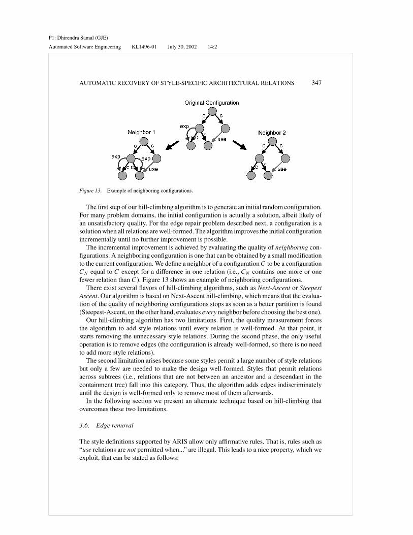
The first step of our hill-climbing algorithm is to generate an initial random configuration.For many problem domains, the initial configuration is actually a solution, albeit likely ofan unsatisfactory quality. For the edge repair problem described next, a configuration is asolution when all relations are well-formed. The algorithm improves the initial configurationincrementally until no further improvement is possible.

The incremental improvement is achieved by evaluating the quality of neighboring con-figurations. A neighboring configuration is one that can be obtained by a small modificationto the current configuration. We define a neighbor of a configuration C to be a configurationCN equal to C except for a difference in one relation (i.e., CN contains one more or onefewer relation than C). Figure 13 shows an example of neighboring configurations.

There exist several flavors of hill-climbing algorithms, such as Next-Ascent or SteepestAscent. Our algorithm is based on Next-Ascent hill-climbing, which means that the evalua-tion of the quality of neighboring configurations stops as soon as a better partition is found(Steepest-Ascent, on the other hand, evaluates every neighbor before choosing the best one).

Our hill-climbing algorithm has two limitations. First, the quality measurement forcesthe algorithm to add style relations until every relation is well-formed. At that point, itstarts removing the unnecessary style relations. During the second phase, the only usefuloperation is to remove edges (the configuration is already well-formed, so there is no needto add more style relations).

The second limitation arises because some styles permit a large number of style relationsbut only a few are needed to make the design well-formed. Styles that permit relationsacross subtrees (i.e., relations that are not between an ancestor and a descendant in thecontainment tree) fall into this category. Thus, the algorithm adds edges indiscriminatelyuntil the design is well-formed only to remove most of them afterwards.

In the following section we present an alternate technique based on hill-climbing thatovercomes these two limitations.

3.6. Edge removal

The style definitions supported by ARIS allow only affirmative rules. That is, rules such as“use relations are not permitted when...” are illegal. This leads to a nice property, which weexploit, that can be stated as follows:




If there exists at least one solution to the edge repair problem for a system with respectto a style specification, the configuration that contains every possible reparable relationwill be one of the solutions.

It is easy to see why this property holds true. Relations can only make other relationswell-formed. Starting from the empty configuration, we can make the use relations well-formed by adding style relations. Note that only reparable relations (i.e., relations that areeither well-formed or can be made well-formed) are added. When no more relations can beadded we are in one of the following situations:

– The configuration is still ill-formed (i.e., it still contains ill-formed relations). This meansthere is no possible solution to this particular edge repair problem.

– The configuration is well-formed.

The edge removal technique starts from the fully reparable configuration for a givenstyle definition and system structure graph. It then removes relations one at a time until nomore relations can be removed without making the configuration ill-formed. Edge removaleliminates the first phase of the hill-climbing technique, by starting from an already well-formed configuration. Moreover, since the only allowable action is to remove relations, thealgorithm does not need to analyze neighboring configurations that are obtained by addingrelations.

However, if the style allows too many edges, the algorithm will have to start from avery large configuration, only to possibly determine that the actual solution requires a fewrelations to be well-formed. Nonetheless, we have found that edge repair is a good contenderagainst hill-climbing. In the following section we compare the two algorithms.

3.7. Comparison of techniques

Styles can be classified into two broad categories: those that allow relations between differentsubtrees (e.g., import) and those that allow relations only between ancestors and descendantsin the containment hierarchy (e.g., export). These categories are meaningful because theydiffer in the order of magnitude of relations that they permit. The first category allowsroughly O(N 2) relations. It is easy to understand why, since the system contains N modulesand subsystems. On the other hand, the second category allows O(N log2 N ) relations. Tounderstand why, consider that each branch in the containment tree contains roughly log Nnodes and there are roughly N/2 unique branches from the root to the leaves. Thus, thereare log2 N possible relations per branch, for a total of O( N

2 log2 N ) relations. To understandthe implications of these results, consider a system with 80 nodes. A category 1-style wouldallow roughly 6,400 nodes, whereas a category 2-style would allow roughly 145 nodes.

The Export style we have been using so far is an example of a style that belongs to thesecond category. We next define the Tube style, which belongs to the first category.

The Tube style (Holt and Mancoridis, 1994; Mancoridis and Holt, 1996) is based on thepremise that a subsystem S1 can see another subsystem S2 if S1 is connected via a tube toS2. Two systems can be connected by a tube if they are proper siblings or if their parentsare connected by tubes according to the style definition given in figure 14.




Figure 14. Specification of tube style.

We ran the two algorithms on a Pentium II 450 MHz PC using both the Export and Tubestyle on several systems which we briefly describe below. The number of modules andsubsystems in each system is specified between parentheses.

– Compiler (19): Turing language compiler– Mini Tunis (32): Experimental operating system– Grappa (117): Graph visualization and drawing tool– Incl (212): Subsystem from a source code analysis system

The results are summarized in Table 2. Tests where the duration is N/A were stoppedbefore they finished because they were taking longer than reasonable (i.e., in the order ofhundreds of hours).

Usually a few relations are enough to make a configuration well-formed, so it seemslikely that hill-climbing and edge removal will perform differently depending on the typeof style definition (i.e., hill-climbing might beat edge removal in some cases and vice versa).

Table 2. Comparison of techniques.a

Tube Export

Hill-climbing Edge removal Hill-climbing Edge removal

Compiler 15.73 4.26 0.19 0.14

Minitunis 131.55 25.38 0.8 0.46

Grappa N/A 59721.84 8.5 3.67

Incl N/A N/A 25.72 9.2

aNote: Times are measured in seconds.




However, if we analyze the situation in more detail, we see why edge removal performedbetter in our tests.

It is clear that with styles like Export, which allow only a few of the total possible relations,edge removal performs better than hill-climbing. The situation is not so evident for styleslike Tube, which allow large numbers of relations to occur. We noticed from the tests,however, that hill-climbing would add a huge number of edges (near the maximum numberof allowed edges) before starting to remove unnecessary relations. Moreover, hill-climbingmust always consider a number of neighbors given by the maximum number of allowedrelations, unlike edge removal, which considers only as many neighbors as the number ofactual relations in the configuration.

3.8. Rule checking

In the previous sections we described algorithms for finding a reasonable solution to theedge repair problem. The evaluation of the fitness function is at the core of these techniquesand is the main performance bottleneck. Thus, it is important to come up with an efficientimplementation for the fitness function evaluation.

Recall from Section 3.5 that fitness evaluation involves counting the number of well-formed and ill-formed relations in a configuration. This requires testing each relation forwell-formedness or, in other words, finding out if they satisfy at least one of the permissionrules in the style specification.

Permission rules represent subgraph patterns and are defined by a set of nodes and edges.Each edge has a type, namely, that of the of relation it represents and a flag that stateswhether it is a transitive closure relation or not. A special edge in the graph—the targetcorresponds to the relation that is allowed to occur if the pattern described by the permissionrule is met. Definition rules are similar to permission rules except that their semantics statethat a relation is defined or inferred if the subgraph pattern is met.

The problem of checking if a relation is well-formed can be reduced to a pattern matchof the rule against the structure graph. The match is performed according to the followingrules:

– Each node in the pattern matches a single node in the structure graph.– Each non-transitive edge in the pattern matches a single edge of the appropriate type and

direction.– Each transitive edge in the pattern matches a path formed by 0 or more edges of the

appropriate type and direction.

Figure 15 shows some examples of valid and invalid matches.Before describing the matching algorithm we will briefly show why a brute force approach

is not feasible. A brute force method would test all possible combinations of nodes (or edges)in the structure graph that can be assigned to the nodes (and edges) in the pattern. If N is thenumber of nodes in the structure graph and n the number of nodes in the pattern, the totalnumber of such combinations is given by the combinatorial ( N

n ). Checking a simple rule likePERMIT(1) in figure 14 on a small-sized system (e.g., 50 nodes) would require generating




Figure 15. Examples of subgraph pattern matching.

and analyzing 230, 300 combinations, which could be performed by a fast processor in littletime. However, the computation becomes impractical for a system ten times bigger (i.e.,500 nodes), as more than 2 billion combinations must be generated and evaluated.

Since rules must be matched several times per evaluation of the objective function, the taskbecomes a major performance bottleneck even for small systems. A more efficient algorithmcan be devised once the characteristics of the rule matching process are contemplated. Inparticular,

– since nodes in the pattern can be matched to nodes in the structure graph as long asthe same number and types of edges come into and out of each node, many potentialassignments can be discarded right away.

– Moreover, the nodes at the endpoints of the target relation are fixed as far as the matchingprocess is concerned, effectively anchoring the pattern to the structure graph. Not coin-cidentally, the matching algorithm needs to take into account only the subgraph coveredby expanding the pattern from the anchor points. In most cases, especially due to thehierarchical nature of the containment relationship and the strict constraints imposed bythe style rules, this subgraph is relatively small.

Based on these considerations, we next describe the subgraph pattern-matching algorithm.

3.9. Subgraph pattern matching

We first describe the pattern-matching algorithms and then, provide an example that shouldclarify any questions pertaining to these algorithms.

The algorithm is constructed as a depth-first search method. Each state is defined by theset of fixed nodes, or nodes in the pattern that have already been assigned a match, and theset of free nodes, or nodes in the pattern that have not been assigned a match yet. The goalof the search is to find a state where the set of free nodes is empty.




Since the match is performed to check the well-formedness of a specific relation, thesource and destination nodes for the target relation are fixed initially. The initial state isconstructed by adding these two nodes to the set of fixed nodes and the rest of the nodes tothe free node set.

The next state is reached by assigning a match to any free node in the current state. Thisnode now becomes part of the set of fixed nodes.

We now proceed to describe the steps of the algorithm.

– Push the initial state onto a stack S.– Repeat until S is empty or the goal is found.

• Pop the first element, E , from S.• Check if E is the goal (i.e., check if the set of free nodes in E is empty).• If it is, do nothing.• If it is not the goal, expand E’s successor states and push them onto S. To generate the

successor states,

1. First choose a free node N . This node should be connected to one or more of thefixed nodes in order to constrain the number of allowable matches.

2. Then, find the set of nodes in the structure graph that can be matched to N . Thealgorithm for doing so will be described later on.

3. Finally, create a new state for each possible node assignment N can take.

– If the goal was found, return “well-formed”.– If S is empty, return “ill-formed”.

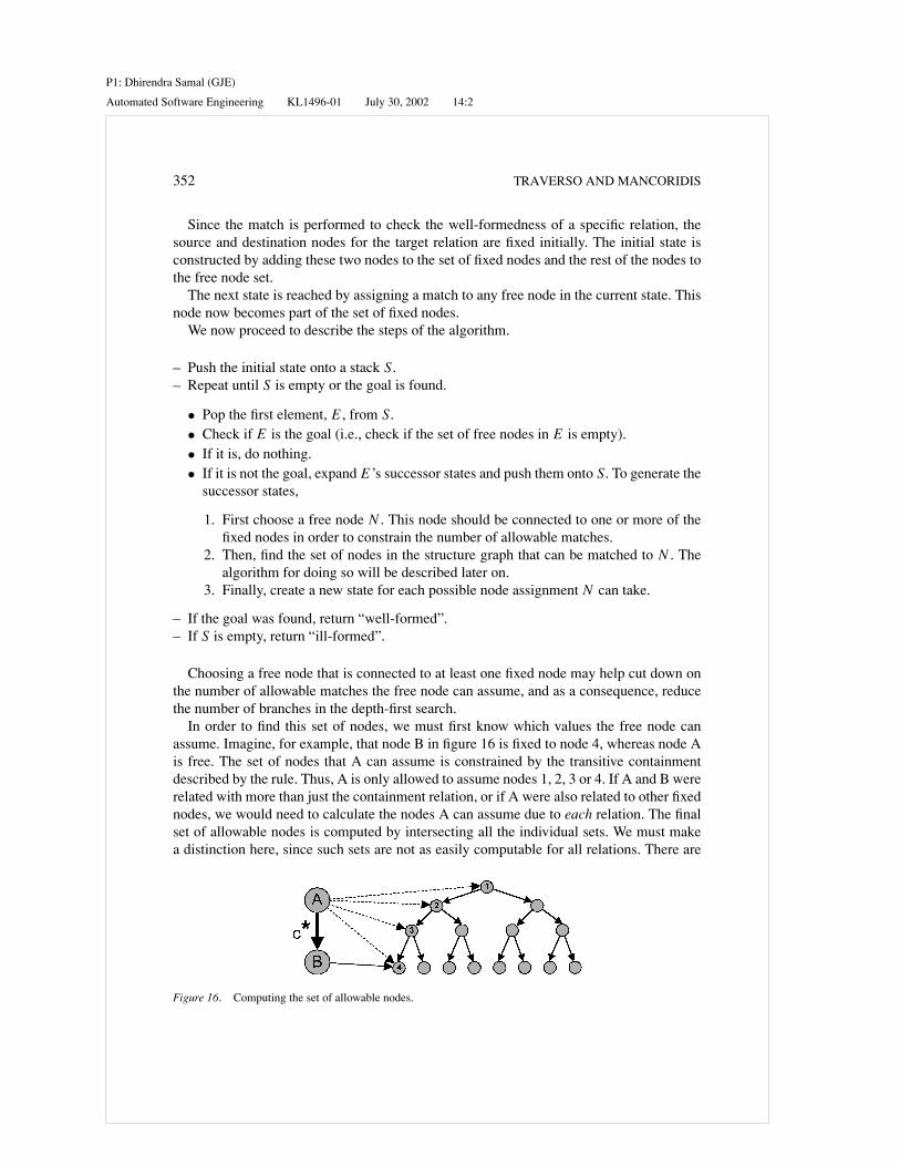
Choosing a free node that is connected to at least one fixed node may help cut down onthe number of allowable matches the free node can assume, and as a consequence, reducethe number of branches in the depth-first search.

In order to find this set of nodes, we must first know which values the free node canassume. Imagine, for example, that node B in figure 16 is fixed to node 4, whereas node Ais free. The set of nodes that A can assume is constrained by the transitive containmentdescribed by the rule. Thus, A is only allowed to assume nodes 1, 2, 3 or 4. If A and B wererelated with more than just the containment relation, or if A were also related to other fixednodes, we would need to calculate the nodes A can assume due to each relation. The finalset of allowable nodes is computed by intersecting all the individual sets. We must makea distinction here, since such sets are not as easily computable for all relations. There are

Figure 16. Computing the set of allowable nodes.




four types of relationships, namely, containment, inequality, those allowed by permissionrules and those that are inferred from definition rules.

Containment relations and those relations allowed by permission rules exist in the struc-ture graph explicitly (i.e., they are added and removed by the edge repair algorithm). There-fore, finding the set of allowable nodes is straightforward.

Relations inferred from definition rules, however, do not exist explicitly in the graph. Therelations must be induced from the rules before the set of allowable nodes can be computed.Since induction is quite hard to compute, probably more so than just checking to see ifeach possible relation exists, we will constrain the number of allowable nodes due to theserelations by checking every possible relation and discarding those that do not satisfy the rule.

Finally, it is clear that inequality relations produce sets of N − 1 nodes, where N is thesize of the structure graph, since only one node in the graph can be equal to the fixed node.

Now that we have characterized the four types of relations we will sketch the algorithmfor finding the allowable set of nodes for a free node.

1. Find the set of nodes Si due to either containment relations or relations allowed bypermission rules between the free node and any fixed node. If no relations can be found,make Si = V , where V is the set of all nodes in the structure graph.

2. Compute the intersection S = ∩i Si .3. Remove from S the nodes that violate any inequality relation between the free node and

any fixed node.4. Remove from S the nodes that do not satisfy the inferred relations between the free nodes

and any fixed node. This will involve triggering a parallel pattern-matching process forthe relation in question.

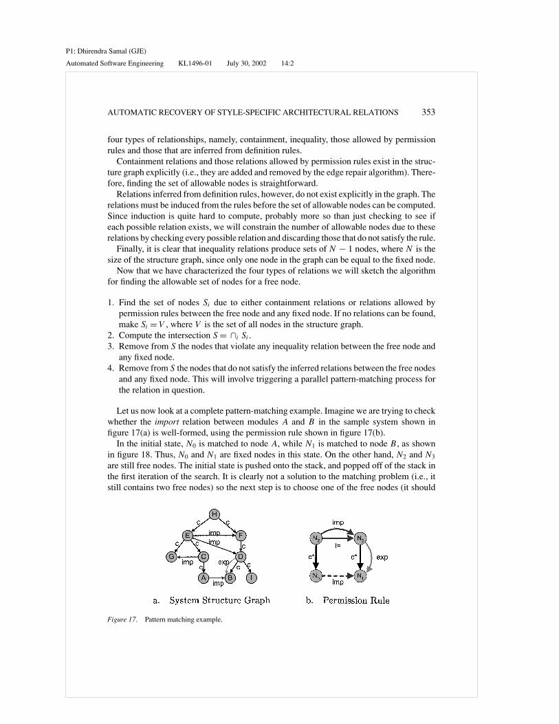
Let us now look at a complete pattern-matching example. Imagine we are trying to checkwhether the import relation between modules A and B in the sample system shown infigure 17(a) is well-formed, using the permission rule shown in figure 17(b).

In the initial state, N0 is matched to node A, while N1 is matched to node B, as shownin figure 18. Thus, N0 and N1 are fixed nodes in this state. On the other hand, N2 and N3

are still free nodes. The initial state is pushed onto the stack, and popped off of the stack inthe first iteration of the search. It is clearly not a solution to the matching problem (i.e., itstill contains two free nodes) so the next step is to choose one of the free nodes (it should

Figure 17. Pattern matching example.




Figure 18. Example of a search tree traversed by the pattern matching algorithm.

be connected to at least one fixed node). We pick, for instance, N2. Since the only relationbetween N2 and a connected node is the transitive containment c∗, the set of nodes thatcan be assigned to N2 are A, C, E, and H . The current state is then expanded into foursuccessor states, each with a different assignment for node N2. These are pushed onto thestack.

In the next iteration, the first state is popped off of the stack. In our example, this statecorresponds to the leftmost picture in figure 18. The only free node in this case is N3, sothere is no choice other than to pick it. There are four relations between N3 and fixed nodes,namely, an import, an export, a transitive containment and an inequality relation. The setsof allowable nodes for each relation are:

– {B}, for the import relation between N2 (which is fixed to node A) and N3.– {B, D, F, H} for the transitive containment between N3 and N1 (which is fixed to node B).– {D} for the export relation between N3 and N1.

The intersection of the three sets is the empty set (regardless the remaining inequalityrelation), so we conclude that there is no possible assignment to node N3 from the currentstate.

Next, the top element in the stack, which corresponds to the second diagram in figure 18,is popped off. We proceed to try to find the permissible assignments to node N3. Since theset of nodes given by the import relation between node N2 (which is fixed to C) and N3 isempty (i.e., C does not import anything), we conclude that there is no possible assignmentto N3 from the current state.




However, when we analyze the following case, we notice that the sets of allowable nodesfor each relation are:

– {F, D}, for the import relation between N2 (which is fixed to node E) and N3.– {B, D, F, H} for the transitive containment between N3 and N1 (which is fixed to node B).– {D} for the export relation between N3 and N1.

The intersection of the three sets is D, and since D is not equal to N2’s value, we concludethat D is the only valid assignment. The new state is now pushed onto the stack.

In the final iteration, the previously pushed state is popped from the stack and, sinceit is a solution to the algorithm, the algorithm finishes and returns the “well-formed”message.

The rule-matching algorithm can also be used, with minor modifications, to check whetherrelations are reparable. In order for a relation to be reparable, there must potentially existat least one configuration of reparable relations that can make it well-formed.

4. Case study

In Section 2.2 we showed how several reverse-engineering tools, such as source codeanalyzers, clustering tools and our edge repair utility can be used together. In this sectionwe describe how we used these tools to gain some insight on the design of Jakarta Project’sTomcat, an open-source servlet container written in Java. The purpose of a servlet containeris to take care of servlet and JSP requests on behalf of a web server, while the web servertakes care of other HTTP requests. We also highlight how the results of our study canprovide some guidance for prospective maintainers of Tomcat.

Without the help of reverse engineering tools, understanding the structure of the Tomcatand how its components relate to each other can be quite hard. It is important that newdevelopers and future maintainers be able to understand the system well enough to be ableto make changes without breaking the application, especially since anybody can contributecode to the project due to its open-source nature.

Before using our tool, we first obtained a module dependency graph of Tomcat andclustered it into a module hierarchy. The MDG was obtained using Chava (Korn et al.,1999). Modules in this MDG represent classes in Tomcat, whereas relations representvariable references, method calls and class inheritance relations. The clustering we producedis based on the package structure of the application. In Java, package names are composedof words separated by dots. Although there is no inherent hierarchical structure to thepackage system, developers usually create names that resemble containment hierarchies.For instance, javax.swing.event is regarded as being a child of javax.swing. Similarly, thepackage structure in Tomcat resembles a hierarchical organization, with package namessuch as org.apache.tomcat, org.apache.tomcat.core or org.apache.jasper.

The cluster tree contains more than 370 nodes, so showing it here is not feasible. In thecourse of this analysis, however, we show relevant portions of the cluster tree, includingstyle-specific relations found by our tool.

We based our analysis on the Export style introduced in Section 1. As we have seen, theExport style allows only one kind of high-level relation, namely, the export relation.




Figure 19. Core subsystem.

The results produced by ARIS allow us to make several observations about the structureof Tomcat. Subsystems that export a high percentage of their contents are particularlynoteworthy, since they might reflect poor design choices. Sometimes, these subsystemsmight contain groups of modules that are used all over the application and are consideredto be libraries. Such situations are not bad, but raise the question of whether those modulescan be split into smaller modules that perform more specific functions and that can beplaced alongside modules that use them. Other times, those situations may occur becausethe modules have been misplaced in the wrong subsystems. Figure 19 shows an exampleof a subsystem that might be acting as a library, judging from its name. Note that mostof the modules in the subsystem are exported, and thus, are visible from the outside oforg.apache.tomcat.core. The thin edges in the diagram represent containment relationsbetween modules and subsystems, whereas thick edges represent export relations.

The existence of export relations, or lack of them, gives us some information on how achange to a module might affect the rest of the system. In particular, if a module is localto a subsystem (i.e., it is not exported), it is clear that making modifications to it shouldnot affect anything outside the subsystem where it belongs. Maintenance efforts can beconcentrated on a small subset of the system. On the other hand, the existence of an exportrelation is an indication that changes to the module may affect a wide range of modulesin the system and thus, care must be taken when modifying the module. For example,if the module ClassRepository in figure 20 needs to be updated, we are sure that onlymodules within the same subsystem can be affected directly. On the other hand, if module




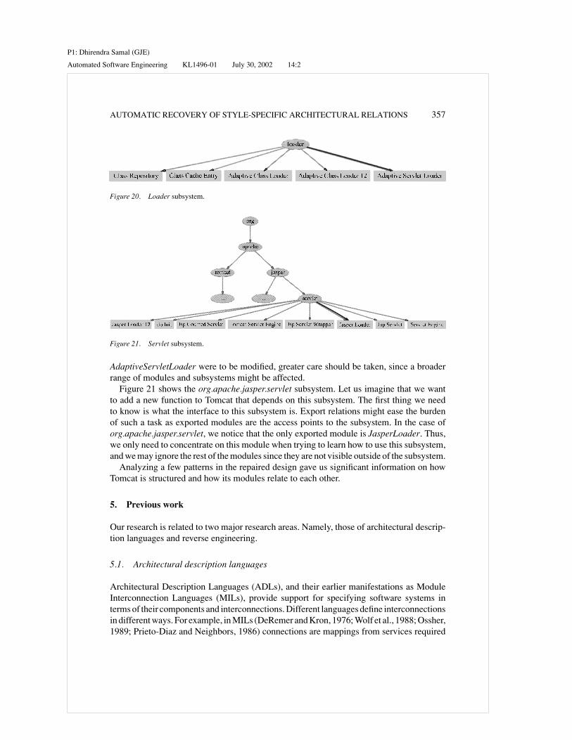
Figure 20. Loader subsystem.

Figure 21. Servlet subsystem.

AdaptiveServletLoader were to be modified, greater care should be taken, since a broaderrange of modules and subsystems might be affected.

Figure 21 shows the org.apache.jasper.servlet subsystem. Let us imagine that we wantto add a new function to Tomcat that depends on this subsystem. The first thing we needto know is what the interface to this subsystem is. Export relations might ease the burdenof such a task as exported modules are the access points to the subsystem. In the case oforg.apache.jasper.servlet, we notice that the only exported module is JasperLoader. Thus,we only need to concentrate on this module when trying to learn how to use this subsystem,and we may ignore the rest of the modules since they are not visible outside of the subsystem.

Analyzing a few patterns in the repaired design gave us significant information on howTomcat is structured and how its modules relate to each other.

5. Previous work

Our research is related to two major research areas. Namely, those of architectural descrip-tion languages and reverse engineering.

5.1. Architectural description languages

Architectural Description Languages (ADLs), and their earlier manifestations as ModuleInterconnection Languages (MILs), provide support for specifying software systems interms of their components and interconnections. Different languages define interconnectionsin different ways. For example, in MILs (DeRemer and Kron, 1976; Wolf et al., 1988; Ossher,1989; Prieto-Diaz and Neighbors, 1986) connections are mappings from services required




by one component to services provided by another component. In ADLs (Shaw et al., 1995;Dellarocas, 1997) connections define the protocols for integrating sets of components.

Our work is not tied to any particular notation for describing software designs. It onlyassumes that the notation can model designs as graphs.

5.2. Reverse engineering

Much of the research in reverse engineering deals with extracting high-level design informa-tion by analyzing legacy source code and documentation. Source code analysis tools, suchas CIA for C (Krishnamurthy, 1995), Acacia for C++ (Chen et al., 1997) and Chava forJava (Korn et al., 1999), gather information about source code components (e.g., procedures,classes) and the relations between these components (e.g., procedure invocation, class in-heritance). Traditional reverse engineering techniques, such as those by Muller et al. (1992),Schwanke (1991), and Mancoridis et al. (1999) are bottom-up. In these techniques, relatedsource code components are clustered, using a variety of criteria (Muller et al., 1992), intosubsystem decomposition hierarchies.

Current bottom-up techniques are effective in determining how source code componentsare partitioned into subsystem hierarchies. An alternative to traditional bottom-up reverseengineering techniques was developed by Murphy et al. (1995). In this technique, softwareengineers specify multiple views of the software structure manually at any level of detail,and use tools to detect any inconsistencies between the proposed structure and the actualsource code. This technique is aimed at checking design conformance at the source level.The products of this technique are reflexion models, which summarize source models of asoftware systems from the viewpoint of high-level models. Our technique, on the other hand,is aimed at checking conformance at a higher level. Source-level and high-level relationsare validated against a set of stylistic constraints that define patterns of interaction betweenmodules and subsystems.

Thus, our research is intended to complement existing reverse engineering techniques.These techniques produce good subsystem decompositions, but do not produce informationabout high-level relations between the newly formed subsystems.

An alternative method for repairing designs has been suggested by Fahmy et al. (1997),who showed how graph grammars can be used to define well-formed architectures. ViewingISF rules as graph grammar rules, however, implies converting transitive relations into re-cursive graph rewriting rules, which can be cumbersome and less intuitive than the transitiveclosure notation used in ISF.

The Rigi tool (Muller et al., 1993) has a visual notation to capture subsystem-levelabstractions and supports the automatic extraction of subsystem interfaces. These interfacesare similar (in concept) to the Export style. What makes our approach different is that it isbased on a language (i.e., ISF) that can be used to create other styles (not just Export).

6. Summary and future work

We have described a tool that finds missing relations in a system in order to make itsdesign well-formed with respect to a style definition. Style relations provide insight intohow subsystems relate to each other and how their interfaces are composed.




Further research will focus on optimizing the edge repair algorithm. One path to pur-sue, which we believe will provide the best performance enhancement, is to define andimplement incremental algorithms for computing fitness and visibility. An incremental al-gorithm will obviously speed up ARIS, but also allow us to replace the “simplistic visibility”measurement.

Another line of research could be directed toward investigating how to repair designs byre-configuring the system clustering, in addition to finding missing relations. One possibleapproach is to allow containment relations in the system structure graph to be changed duringthe course of the algorithm. Currently, the containment hierarchy remains fixed throughoutthe entire edge-repair process. A different approach might combine the clustering and edgerepair methods into an aggregate algorithm.

Acknowledgments

This research is sponsored by grants CCR-9733569 and CISE-9986105 from the NationalScience Foundation (NSF). Additional support was provided by the research laboratoriesof AT&T, and Sun Microsystems.

Any opinions, findings, and conclusions or recommendations expressed in this materialare those of the authors and do not necessarily reflect the views of the NSF, U.S. Government,AT&T, or Sun Microsystems.

The ARIS binaries, user documentation, and an installation guide can be downloadedfrom http://serg.mcs.drexel.edu/ISF.

References

Biggerstaff, T.J. 1989. Design recovery for maintenance and reuse. IEEE Computer, 22(7):36–49.Chen, Y., Gansner, E.R., and Koutsofios, E. 1997. A C++ data model supporting reachability analysis and dead

code detection. In Proceedings of the European Conference on Software Engineering/Foundations of SoftwareEngineering.

Chikofsky, E.J. and Cross, J.H. 1990. Reverse engineering and design recovery: A taxonomy. IEEE Software,7(1):13–17.

Consens, M.P. and Mendelzon, A.O. 1990. GraphLog: A visual formalism for real life recursion. In Proceedingsof the 9th ACM SIGACT-SIGMOD Symposium on Principles of Database Systems, pp. 404–416.

Dellarocas, C. 1997. A coordination perspective on software system design. In Proceedings of the 9th InternationalConference on Software Engineering and Knowledge Engineering, pp. 318–325.

DeRemer, F. and Kron, H.H. 1976. Programming in the large versus programming in the small. IEEE Transactionson Software Engineering, 2(2):80–86.

Fahmy, H., Holt, R.C., and Mancoridis, S. 1997. Repairing software style using graph grammars. In IBM Pro-ceedings of the Seventh Centre for Advanced Studies Conference (CASCON’97).

Gansner, E., Koutsofios, E., North, S., and Vo, K. 1993. A technique for drawing directed graphs. IEEE Transactionson Software Engineering, 19(3):214–230.

Holt, R.C. and Mancoridis, S. 1994. Using tube graphs to model architectural designs of software systems.Technical Report CSRI-308, Computer Science Research Institute, University of Toronto.

Korn, J., Chen, Y., and Koutsofios, E. 1999. Chava: Reverse engineering and tracking of Java applets. In Proceedingsof the 6th Working Conference on Reverse Engineering, pp. 314–325.

Krishnamurthy, B. 1995. Practical Reusable Unix Software. New York: John Wiley & Sons.Mancoridis, S. 1997. Customizable notations for software design. In Proceedings of the 9th International Confer-

ence on Software Engineering and Knowledge Engineering.




Mancoridis, S. 1998. ISF: A visual formalism for specifying interconnection styles for software design. Inter-national Journal of Software Engineering and Knowledge Engineering, World Scientific Publishing Company,8(4):517–540.

Mancoridis, S. and Holt, R.C. 1996. Recovering the structure of software systems using tube graph interconnectionclustering. In Proceedings of the 1996 International Conference on Software Maintenance.

Mancoridis, S., Mitchell, B.S., Chen, Y., and Gansner, E.R. 1999. Bunch: A clustering tool for the recovery andmaintenance of software system structures. In Proceedings of International Conference of Software Mainte-nance.

Mancoridis, S., Mitchell, B.S., Rorres, C., Chen, Y., and Gansner, E.R. 1998. Using automatic clustering toproduce high-level system organizations of source code. In Proceedings of the 6th Intl. Workshop on ProgramComprehension.

Muller, H., Orgun, M., Tilley, S., and Uhl, J. 1993. A reverse engineering approach to subsystem structureidentification. Journal of Software Maintenance: Research and Practice, 5:181–204.

Muller, H.A., Orgun, M.A., Tilley, S.R., and Uhl, J.S. 1992. Discovering and reconstructing subsystem structuresthrough reverse engineering. Technical Report DCS-201-IR, University of Victoria, August 1992.

Murphy, G., Notkin, D., and Sullivan, K. 1995. Software reflexion models: Bridging the gap between source andhigh-level models. In Proceedings of the ACM SIGSOFT Symposium on Foundations of Software Engineering(FSE’95), Washington, DC, pp. 18–28.

Ossher, H. 1989. A case study in structure specification: A grid description of scribe. IEEE Transactions onAu: pls.provide thepage rangesfor refs.Ossher, 1989and Shawet al., 1995.

Software Engineering, 15(11).Prieto-Diaz, R. and Neighbors, J.M. 1986. Module interconnection languages. The Journal of Systems and Software,

6:307–334.Schwanke, R.W. 1991. An intelligent tool for re-engineering software modularity. In Proceedings of the 13th IEEE

International Conference on Software Engineering, Austin, Texas, pp. 83–92.Shaw, M., DeLine, R., Klien, D.V., Ross, T.L., Young, D.M., and Zalesnik, G. 1995. Abstractions for software

architectures and tools to support them. IEEE Transactions on Software Engineering, 21.Tzerpos, V. and Holt, R.C. 1998. Software botryology, automatic clustering of software systems. In Proceedings

of the International Workshop on Large-Scale Software Composition, pp. 811–818.Wolf., A.L., Clarke, L.A., and Wileden, J.C. 1988. A model of visibility control. IEEE Transactions on Software

Engineering, 14(4):512–520.

on the automatic recovery of style-speciﬁc …spiros/papers/ause02.pdfp1: dhirendra samal (gje)...

Documents