on the accuracy of finite volume and discontinuous...
TRANSCRIPT
INTERNATIONAL JOURNAL FOR NUMERICAL METHODS IN ENGINEERINGInt. J. Numer. Meth. Engng 2000; 00:1–6 Prepared using nmeauth.cls [Version: 2002/09/18 v2.02]
On the accuracy of Finite Volume and Discontinuous Galerkindiscretizations for compressible flow on unstructured grids
X. Nogueiraa, L. Cueto-Felguerosob, I. Colominasa∗, H. Gomeza,c, F. Navarrinaa,M. Casteleiroa
aGroup of Numerical Methods in Engineering, GMNI, Dept. of Applied MathematicsCivil Engineering School, Universidade da Coruna
Campus de Elvina, 15071, A Coruna, Spain
bAerospace Computational Design Laboratory, Dept. of Aeronautics and AstronauticsMassachusetts Institute of Technology
77 Massachusetts Ave., Cambridge, MA 02139
cInstitute for Computational Engineering and SciencesThe University of Texas at Austin
1 University Station, C0200201 E. 24th Street, Austin, TX 78712
SUMMARY
This paper presents a comparison between two high order methods. The first one is a high-orderFinite Volume (FV) discretization on unstructured grids that uses a meshfree method (Moving LeastSquares (MLS)) in order to construct a piecewise polynomial reconstruction and evaluate the viscousfluxes. The second method is a discontinuous Galerkin (DG) scheme. Numerical examples of inviscidand viscous flows are presented and the solutions are compared. The accuracy of both methods, forthe same grid resolution, is similar, although the DG scheme requires a larger number of degrees offreedom than the FV-MLS method.
Copyright c© 2000 John Wiley & Sons, Ltd.
key words: Compressible flow. Finite Volume method. Discontinuous Galerkin method. High-
resolution schemes. High-order methods. Moving Least-Squares approximation. Unstructured grids.
1. INTRODUCTION
The field of Computational Fluid Dynamics has developed greatly during the last decade.The increase of computer capabilities has allowed the possibility of solving progressively morecomplex problems, which require numerical methods with the capability for capturing the flowfeatures in a very accurate way. DNS and LES of turbulent flows, or aeroacoustics simulationsare examples of this kind of problems. In aeroacoustics, for example, an accurate solution of
∗Correspondence to: E.T.S. de Ingenieros de Caminos, Canales y Puertos, Universidade da Coruna, Campusde Elvina, 15071 A Coruna, Spain. Email: [email protected]
Received YesterdayCopyright c© 2000 John Wiley & Sons, Ltd. Revised Today

2X. NOGUEIRA, L. CUETO-FELGUEROSO, I. COLOMINAS, H. GOMEZ, F. NAVARRINA, M. CASTELEIRO
flow field is needed due to the very low magnitude of acoustic waves. Indeed, the use of firstand second order upwind schemes can lead to excessive numerical dissipation that absorbsthe acoustic wave propagation and drives the simulation to a wrong or not accurate enoughsolution. In addition, in problems where turbulent effects play a significant role, the numericalmethod has to avoid interactions with the turbulence model.
Pseudospectral methods and finite differences are the most natural and commonly usednumerical schemes when very high accuracy is needed. They are extremely competitive onsimple or moderately complex geometries, and unbeatable, both in terms of accuracy andefficiency, by unstructured-grid approaches. However, and even though the use of multiblockgrids allows the extension of structured-grid procedures to rather complex geometries, thedevelopment of unstructured-grid methodologies is nowadays perceived as the most promisingcompromise to achieve the dreamed accurate-fast-automated final objective. It is within thiscontext of unstructured-grid methods that the present study originated.
Continuous finite element formulations for fluid dynamics are applicable to a widevariety of flow conditions. Unfortunately, the too frequently required stabilization, with itsassociated numerical dissipation and lack of robustness, has hampered their widespread usefor compressible flow applications.
Finite volume schemes are widely used, including in industrial problems. Nevertheless, theusual order achieved in these simulations is usually two. This is due to the difficulty ofevaluating high order derivatives of the field variables from scattered, point wise information.These derivatives are required for the reconstruction of field variables by Taylor approximation[1, 2, 3]. Moreover, most of multidimensional schemes are extensions of one dimensional solvers,so if the direction of the flow is not normal to the cell interface, dissipation is a fact [4]. Thisdifficulty is overcome by methods that solve the problem with a Lagrangian approach, theso called meshfree or particle methods. In this context, the Smooth Particle Hydrodynamics(SPH) method was first introduced by Gingold and Monaghan [5] in astrophysical applications.For acoustic applications, Eldredge, Colonius and Leonard have used a vortex particlemethod for the calculation of a corotating vortex pair [6]. In [7, 8, 9] a method that usesa meshfree technique (Moving Least Squares (MLS)) has been proposed to calculate highorder derivatives of the field variables, achieving a truly multidimensional high order approachwith a finite volume scheme. In this method, the spatial finite volume discretization uses theMLS approximation as a kind of “shape functions” for unstructured grids.
On the other hand, few years ago, Discontinuous Galerkin schemes have attracted theattention of researchers. This method was first applied in the solution of neutron transportproblems in 1973 by Reed and Hill [10], and has only been recently extended to generalproblems in fluid dynamics [11, 12, 13, 14]. This technique combines the physics of wavepropagation inherent to finite volume methods with the accuracy of high order polynomialapproximations within elements. In opposition to continuous finite elements, this methodallows the solution to be discontinuous between elements. The coupling between elementsis achieved by means of numerical fluxes, as in the finite volume technique. However, thediscontinuous nature of the approximation brings the main drawback of this method: theincreasing number of degrees of freedom.
In this paper we compare two high order methods (the Discontinuous Galerkin (DG) andthe MLS Finite Volume (FV-MLS) schemes) by using numerical tests. For the DG method, wetake third-order polynomials for the reconstruction of the variables. A Taylor reconstructionup to the third derivative is used for the convective terms on the FV-MLS method. Viscous
Copyright c© 2000 John Wiley & Sons, Ltd. Int. J. Numer. Meth. Engng 2000; 00:1–6Prepared using nmeauth.cls
ON THE ACCURACY OF FV AND DG DISCRETIZATIONS FOR COMPRESSIBLE FLOW 3
fluxes are computed directly at the quadrature points with a cubic reconstruction. Therefore,a comparison is made between two fourth-order methods.We study the accuracy of both methods only for cases with smooth solutions. Notice that theFV-MLS method works well in problems with non-smooth solutions [7, 8, 9], by using shocklimiter techniques designed for Finite Volume solvers.
The outline of the paper is as follows. Section 2 presents the governing equations and sections3 and 4 are devoted to numerical formulations. Interpolation methods are examined in section5, whereas accuracy test and representative simulations are exposed and discussed in sections6 and 7. Finally, conclusions are drawn.
2. GOVERNING EQUATIONS
The 2-D Navier-Stokes equations can be written in conservative form as:
∂UUUUUUUUUUUUUU
∂t+
∂(FFFFFFFFFFFFFF x − FFFFFFFFFFFFFFV
x
)
∂x+
∂(FFFFFFFFFFFFFF y − FFFFFFFFFFFFFFV
y
)
∂y= 0 (1)
with
UUUUUUUUUUUUUU =
ρρvx
ρvy
ρE
(2)
FFFFFFFFFFFFFF x =
ρvx
ρv2x + p
ρvxvy
ρvxH
FFFFFFFFFFFFFF y =
ρvy
ρvxvy
ρv2y + p
ρvyH
(3)
FFFFFFFFFFFFFFVx =
0τxx
τxy
vxτxx + vyτxy − qx
FFFFFFFFFFFFFFV
y =
0τxy
τyy
vxτxy + vyτyy − qy
(4)
with
ρE = ρe +12ρ (vvvvvvvvvvvvvv · vvvvvvvvvvvvvv) (5)
H = E +p
ρ(6)
and
τxx = 2µ∂vx
∂x− 2
3µ
(∂vx
∂x+
∂vy
∂y
)
τyy = 2µ∂vy
∂y− 2
3µ
(∂vx
∂x+
∂vy
∂y
)(7)
τxy = µ
(∂vx
∂y+
∂vy
∂x
)
(8)
Copyright c© 2000 John Wiley & Sons, Ltd. Int. J. Numer. Meth. Engng 2000; 00:1–6Prepared using nmeauth.cls
4X. NOGUEIRA, L. CUETO-FELGUEROSO, I. COLOMINAS, H. GOMEZ, F. NAVARRINA, M. CASTELEIRO
In the above expressions, UUUUUUUUUUUUUU is the vector of conserved variables, vvvvvvvvvvvvvv = (vx, vy) is the velocity,µ is the effective viscosity of the fluid, H is the enthalpy, E is the total energy, e is the totalinternal energy and ρ is the density. The notation FFFFFFFFFFFFFF = (FFFFFFFFFFFFFF x, FFFFFFFFFFFFFF y) and FFFFFFFFFFFFFFV =
(FFFFFFFFFFFFFFV
x , FFFFFFFFFFFFFFVy
)will be
used hereafter in reference to the inviscid and viscous fluxes, respectively.The thermal flux (qqqqqqqqqqqqqq = (qx, qy)) is modeled by Fourier’s law:
qx = −λ∂T
∂xqy = −λ
∂T
∂y(9)
Alternative formulations are possible. The authors are working on developing alternativeformulations for the calculation of thermal fluxes based on Cattaneo’s law [15].
It is assumed that the viscosity depends on the temperature according to Sutherland’s law:
µ = µrefTref + S0
T + S0
(T
Tref
)1.5
(10)
where the subindex ref refers to a reference value and S0 = 110.4K is an empirical constant.
3. HIGH-ORDER FINITE VOLUME METHOD
3.1. Overview
The first discretization analyzed in this study is a high-order unstructured-grid finite volumemethod for convection-dominated flows developed by the authors [7, 8, 9]. The key ingredientof this scheme is a point-wise local high-order approximation framework, which provides acontinuous representation of the solution, and thus allows a simple and efficient discretizationof equations with high order terms.
The usual approach of high-order finite volume schemes is pragmatic and bottom-up. Startingfrom an underlying piecewise constant representation, a discontinuous reconstruction of thefield variables is performed at the cell level. An important practical consequence is thatthe discretization of higher order terms requires some kind of recovery procedure, whichis, almost invariably, inconsistent with the aforementioned reconstruction. Our approach issomewhat the opposite. We start from a high-order and highly regular representation of thesolution, obtained by means of Moving Least-Squares approximation [16], and well suitedfor general, unstructured grids. This approach is directly suitable for the discretization ofelliptic/parabolic equations and high order spatial terms. For equations with a predominantlyhyperbolic character, the global representation is broken locally, at the cell level, into apiecewise polynomial reconstruction, which allows to use the powerful finite volume technologyof Godunov-type schemes for hyperbolic problems (e.g. Riemann solvers, limiters).
3.2. General formulation
Consider a system of conservation laws of the form
∂uuuuuuuuuuuuuu
∂t+∇∇∇∇∇∇∇∇∇∇∇∇∇∇ · (FFFFFFFFFFFFFFH +FFFFFFFFFFFFFFE
)= SSSSSSSSSSSSSS in Ω (11)
supplemented with suitable initial and boundary conditions. The fluxes have been genericallysplit into a hyperbolic-like part, FFFFFFFFFFFFFFH , and an elliptic-like part, FFFFFFFFFFFFFFE . Consider, in addition, a
Copyright c© 2000 John Wiley & Sons, Ltd. Int. J. Numer. Meth. Engng 2000; 00:1–6Prepared using nmeauth.cls
ON THE ACCURACY OF FV AND DG DISCRETIZATIONS FOR COMPRESSIBLE FLOW 5
partition of the domain Ω into a set of non-overlapping control volumes or cells, T h = I.Furthermore, we define a reference point (node), xxxxxxxxxxxxxxI inside each cell (the cell centroid).
The spatial representation of the solution is as follows: consider a function uuuuuuuuuuuuuu(xxxxxxxxxxxxxx), given by itspoint values, uuuuuuuuuuuuuuI = uuuuuuuuuuuuuu(xxxxxxxxxxxxxxI), at the cell centroids, with coordinates xxxxxxxxxxxxxxI . The approximate functionuuuuuuuuuuuuuuh(xxxxxxxxxxxxxx) belongs to the subspace spanned by a set of basis functions NI(xxxxxxxxxxxxxx) associated to thenodes, such that uuuuuuuuuuuuuuh(xxxxxxxxxxxxxx) is given by
uuuuuuuuuuuuuuh(xxxxxxxxxxxxxx) =nxxxxxxxxxxxxxx∑
j=1
Nj(xxxxxxxxxxxxxx)uuuuuuuuuuuuuuj (12)
which states that the approximation at a point xxxxxxxxxxxxxx is computed using certain nxxxxxxxxxxxxxx surroundingnodes. This set of nodes is referred to as the cloud or stencil associated to the evaluationpoint xxxxxxxxxxxxxx. In particular, the above approximation is constructed using Moving Least-Squares(MLS) approximation [16]. Note that, using MLS, the approximate function uuuuuuuuuuuuuuh(xxxxxxxxxxxxxx) is not apolynomial in general. An interesting feature of this MLS approach is the centered character ofthe approximation, thus avoiding the spatial bias which is often found in patch-based piecewisepolynomial interpolation.
Consider now the integral form of the system of conservation laws (11) which, for eachcontrol volume I, reads
∫
ΩI
∂uuuuuuuuuuuuuu
∂tdΩ +
∫
ΓI
(FFFFFFFFFFFFFFH +FFFFFFFFFFFFFFE) · nnnnnnnnnnnnnn dΓ =
∫
ΩI
SSSSSSSSSSSSSS dΩ (13)
Introducing the component-wise reconstructed function uuuuuuuuuuuuuuh, the spatially discretizedcounterpart of (13) reads
∫
ΩI
∂uuuuuuuuuuuuuuh
∂tdΩ +
∫
ΓI
(FFFFFFFFFFFFFFhH +FFFFFFFFFFFFFFhE) · nnnnnnnnnnnnnn dΓ =
∫
ΩI
SSSSSSSSSSSSSSh dΩ (14)
A direct evaluation of the fluxes in (14) is possible and efficient when the inherent dissipationmechanism is strong enough to overpower the convective terms. In convection-dominatedproblems, where the character of the equations is predominantly hyperbolic, this centeredapproach can lead to unstable computations. For this latter type of problems, we introducea “broken” reconstruction, uuuuuuuuuuuuuuhb
I , which approximates uuuuuuuuuuuuuuh(xxxxxxxxxxxxxx) (and, therefore, uuuuuuuuuuuuuu(xxxxxxxxxxxxxx)) locallyinside each cell I, and is discontinuous across cell interfaces [7, 9]. In general, we requirethe order of accuracy of the broken reconstruction to be the same as that of the originalcontinuous reconstruction. One possible choice is to use Taylor series expansions; a quadraticreconstruction inside cell I, for example, would read
uuuuuuuuuuuuuuhbI (xxxxxxxxxxxxxx) = uuuuuuuuuuuuuuh
I +∇∇∇∇∇∇∇∇∇∇∇∇∇∇uuuuuuuuuuuuuuhI · (xxxxxxxxxxxxxx− xxxxxxxxxxxxxxI) +
12
(xxxxxxxxxxxxxx− xxxxxxxxxxxxxxI)T
HHHHHHHHHHHHHHh (xxxxxxxxxxxxxx− xxxxxxxxxxxxxxI) (15)
where the gradient ∇∇∇∇∇∇∇∇∇∇∇∇∇∇uuuuuuuuuuuuuuhI and the Hessian matrix HHHHHHHHHHHHHHh involve the successive derivatives of
the continuous reconstruction uuuuuuuuuuuuuuh(xxxxxxxxxxxxxx), which are evaluated at the cell centroids using MLS.This dual continuous/discontinuous reconstruction of the solution is crucial in order to obtainaccurate and efficient numerical schemes for mixed parabolic/hyperbolic problems. The cell-wise broken reconstruction defined here is actually a piecewise continuous approximation touuuuuuuuuuuuuuh. The advantage is that it allows to make use of Riemann solvers, limiters, and other
Copyright c© 2000 John Wiley & Sons, Ltd. Int. J. Numer. Meth. Engng 2000; 00:1–6Prepared using nmeauth.cls
6X. NOGUEIRA, L. CUETO-FELGUEROSO, I. COLOMINAS, H. GOMEZ, F. NAVARRINA, M. CASTELEIRO
standard finite volume technologies, while keeping some consistency in terms of functionalrepresentation. Thus, the general continuous reconstruction is used to evaluate the viscous(elliptic-like) fluxes, whereas its discontinuous approximation is used to evaluate the inviscid(hyperbolic-like) fluxes.
The final semidiscrete scheme for the continuous/discontinuous approach can be written as
∫
ΩI
∂uuuuuuuuuuuuuuh
∂tdΩ +
∫
ΓI
HHHHHHHHHHHHHH(uuuuuuuuuuuuuuhb+, uuuuuuuuuuuuuuhb−) dΓ +∫
ΓI
FFFFFFFFFFFFFFhE · nnnnnnnnnnnnnn dΓ =∫
ΩI
SSSSSSSSSSSSSSh dΩ (16)
where HHHHHHHHHHHHHH(uuuuuuuuuuuuuuhb+, uuuuuuuuuuuuuuhb−) is a suitable numerical flux.
3.3. Moving Least Squares (MLS) approximation
Consider a function u(xxxxxxxxxxxxxx) defined in a domain Ω. The basic idea of the MLS approach is toapproximate u(xxxxxxxxxxxxxx), at a given point xxxxxxxxxxxxxx, through a weighted least-squares fitting of u(xxxxxxxxxxxxxx) in aneighborhood of xxxxxxxxxxxxxx as
u(xxxxxxxxxxxxxx) ≈ u(xxxxxxxxxxxxxx) =m∑
i=1
pi(xxxxxxxxxxxxxx)αi(zzzzzzzzzzzzzz)∣∣∣zzzzzzzzzzzzzz=xxxxxxxxxxxxxx
= ppppppppppppppT (xxxxxxxxxxxxxx)αααααααααααααα(zzzzzzzzzzzzzz)∣∣∣zzzzzzzzzzzzzz=xxxxxxxxxxxxxx
(17)
ppppppppppppppT (xxxxxxxxxxxxxx) is an m-dimensional polynomial basis and αααααααααααααα(zzzzzzzzzzzzzz)∣∣∣zzzzzzzzzzzzzz=xxxxxxxxxxxxxx
is a set of parameters to bedetermined, such that they minimize the following error functional
J(αααααααααααααα(zzzzzzzzzzzzzz)
∣∣∣zzzzzzzzzzzzzz=xxxxxxxxxxxxxx
)=
∫
yyyyyyyyyyyyyy∈ΩxxxxxxxxxxxxxxW (zzzzzzzzzzzzzz − yyyyyyyyyyyyyy, h)
∣∣∣zzzzzzzzzzzzzz=xxxxxxxxxxxxxx
[u(yyyyyyyyyyyyyy)− ppppppppppppppT (yyyyyyyyyyyyyy)αααααααααααααα(zzzzzzzzzzzzzz)
∣∣∣zzzzzzzzzzzzzz=xxxxxxxxxxxxxx
]2
dΩxxxxxxxxxxxxxx (18)
where W (zzzzzzzzzzzzzz − yyyyyyyyyyyyyy, h)∣∣∣zzzzzzzzzzzzzz=xxxxxxxxxxxxxx
is a kernel with compact support (denoted by Ωxxxxxxxxxxxxxx) centered at zzzzzzzzzzzzzz = xxxxxxxxxxxxxx.The parameter h is the smoothing length, which is a measure of the size of the support Ωxxxxxxxxxxxxxx.The minimization of J leads to:
∫
yyyyyyyyyyyyyy∈Ωxxxxxxxxxxxxxxpppppppppppppp(yyyyyyyyyyyyyy)W (zzzzzzzzzzzzzz − yyyyyyyyyyyyyy, h)
∣∣∣zzzzzzzzzzzzzz=xxxxxxxxxxxxxx
u(yyyyyyyyyyyyyy)dΩxxxxxxxxxxxxxx = MMMMMMMMMMMMMM(xxxxxxxxxxxxxx)αααααααααααααα(zzzzzzzzzzzzzz)∣∣∣zzzzzzzzzzzzzz=xxxxxxxxxxxxxx
(19)
MMMMMMMMMMMMMM(xxxxxxxxxxxxxx)is the moment matrix, defined by:
MMMMMMMMMMMMMM(xxxxxxxxxxxxxx) =∫
yyyyyyyyyyyyyy∈Ωxxxxxxxxxxxxxxpppppppppppppp(yyyyyyyyyyyyyy)W (zzzzzzzzzzzzzz − yyyyyyyyyyyyyy, h)
∣∣∣zzzzzzzzzzzzzz=xxxxxxxxxxxxxx
ppppppppppppppT (yyyyyyyyyyyyyy) (20)
In numerical computations the global domain Ω is represented by a set of nodes or particles.The integral in (18) is thus evaluated using those nodes inside Ωxxxxxxxxxxxxxx as quadrature points. Indiscrete form, the set of parameters αααααααααααααα that minimize the functional J are given by
αααααααααααααα(zzzzzzzzzzzzzz)∣∣∣zzzzzzzzzzzzzz=xxxxxxxxxxxxxx
= MMMMMMMMMMMMMM−1(xxxxxxxxxxxxxx)PPPPPPPPPPPPPPΩxxxxxxxxxxxxxxWWWWWWWWWWWWWWV (xxxxxxxxxxxxxx)uuuuuuuuuuuuuuΩxxxxxxxxxxxxxx (21)
where the vector uuuuuuuuuuuuuuΩxxxxxxxxxxxxxx contains the pointwise values of the function to be reproduced (u (xxxxxxxxxxxxxx)),at the nxxxxxxxxxxxxxx nodes inside Ωxxxxxxxxxxxxxx.Introducing (21) in (17), the interpolation structure can be identified as
Copyright c© 2000 John Wiley & Sons, Ltd. Int. J. Numer. Meth. Engng 2000; 00:1–6Prepared using nmeauth.cls
ON THE ACCURACY OF FV AND DG DISCRETIZATIONS FOR COMPRESSIBLE FLOW 7
u(xxxxxxxxxxxxxx) = ppppppppppppppT (xxxxxxxxxxxxxx)MMMMMMMMMMMMMM−1(xxxxxxxxxxxxxx)PPPPPPPPPPPPPPΩxxxxxxxxxxxxxxWWWWWWWWWWWWWW (xxxxxxxxxxxxxx)uuuuuuuuuuuuuuΩxxxxxxxxxxxxxx = NNNNNNNNNNNNNNT (xxxxxxxxxxxxxx)uuuuuuuuuuuuuuΩxxxxxxxxxxxxxx =nxxxxxxxxxxxxxx∑
j=1
Nj(xxxxxxxxxxxxxx)uj (22)
In analogy to finite elements, the approximation is written in terms of the MLS “shapefunctions”
NNNNNNNNNNNNNNT (xxxxxxxxxxxxxx) = ppppppppppppppT (xxxxxxxxxxxxxx)MMMMMMMMMMMMMM−1(xxxxxxxxxxxxxx)PPPPPPPPPPPPPPΩxxxxxxxxxxxxxxWWWWWWWWWWWWWW (xxxxxxxxxxxxxx) (23)
The basis of functions used in this study comprise scaled and locally defined monomials.Thus, in order to reconstruct a one-dimensional function at a location xI , we use basis of theform
pppppppppppppp(xxxxxxxxxxxxxx) =
(1
x− xI
h
(x− xI
h
)2
. . .
(x− xI
h
)p)T
(24)
The functional basis pppppppppppppp(xxxxxxxxxxxxxx) is strongly related to the accuracy of the MLS fit. For a pth order MLSfit (pth order complete polynomial basis) and general, irregularly spaced points, the nominalorder of accuracy for the approximation of an sth order gradient is roughly (p − s + 1). Ingeneral, any linear combination of the functions included in the basis is exactly reproducedby the MLS approximation. In multidimensions we follow the same idea of p-complete basis,constructed using products of scaled and locally defined monomials.
The MLS shape functions are data independent and, therefore, for fixed grids they need tobe computed only once at the preprocessing phase. In order to prevent the moment matrixMMMMMMMMMMMMMM from being singular or ill-conditioned, the cloud of neighbors must fulfill certain “goodneighborhood” requirements. The definition of the cloud (the MLS stencil) for each evaluationpoint is a crucial issue that requires careful attention. The selection process must be suitablefor general unstructured grids, and the stencil should be as compact as possible for the sake ofcomputational efficiency and physical meaning. Note that these stencils are typically centeredaround the node, and thus the MLS approximation avoids the spatial bias which is often foundin patch-based piecewise polynomial approximations.
The particles needed for the application of the method are identified with the centroids ofevery cell of the grid. In the case of boundary cells, we add nodes (ghost nodes) placed in themiddle of the edge wall.
The approximate derivatives of u (xxxxxxxxxxxxxx) can be expressed in terms of the derivatives of theMLS shape functions, which are functions of the derivatives of the polynomial basis pppppppppppppp(xxxxxxxxxxxxxx−xxxxxxxxxxxxxxI
h )and the derivatives of CCCCCCCCCCCCCC(xxxxxxxxxxxxxx) [7, 9]. For example, the first, second and third-order derivatives ofu(xxxxxxxxxxxxxx), evaluated at xxxxxxxxxxxxxxI , are given by
∂u (xxxxxxxxxxxxxx)∂xα
∣∣∣∣xxxxxxxxxxxxxx=xxxxxxxxxxxxxxI
≈nxxxxxxxxxxxxxxI∑
j=1
uj∂Nj (xxxxxxxxxxxxxx)
∂xα
∣∣∣∣xxxxxxxxxxxxxx=xxxxxxxxxxxxxxI
∂2u (xxxxxxxxxxxxxx)∂xα∂xβ
∣∣∣∣xxxxxxxxxxxxxx=xxxxxxxxxxxxxxI
≈nxxxxxxxxxxxxxxI∑
j=1
uj∂2Nj (xxxxxxxxxxxxxx)∂xα∂xβ
∣∣∣∣xxxxxxxxxxxxxx=xxxxxxxxxxxxxxI
Copyright c© 2000 John Wiley & Sons, Ltd. Int. J. Numer. Meth. Engng 2000; 00:1–6Prepared using nmeauth.cls
8X. NOGUEIRA, L. CUETO-FELGUEROSO, I. COLOMINAS, H. GOMEZ, F. NAVARRINA, M. CASTELEIRO
∂3u (xxxxxxxxxxxxxx)∂xα∂xβ
∣∣∣∣xxxxxxxxxxxxxx=xxxxxxxxxxxxxxI
≈nxxxxxxxxxxxxxxI∑
j=1
uj∂3Nj (xxxxxxxxxxxxxx)∂xα∂xβ
∣∣∣∣xxxxxxxxxxxxxx=xxxxxxxxxxxxxxI
(25)
In this work we have used a polynomial cubic basis in (24), so we can compute until thethird derivative. Therefore the maximum order of the FV-MLS scheme we can get with thisbasis is four. The polynomial basis also defines the minimum number of neighbors (nodes)needed in the stencil for the MLS approximation. Thus, for the cubic basis and 2D problemsat least 10 points are required. However, it is recommended to increase slightly this numberin order to avoid a ill conditioning of the moment matrix MMMMMMMMMMMMMM . On the other hand, it is possibleto obtain higher orders by using quartic or higher basis. In this case, the number of points inthe stencil needs to be increased. In practical applications, however, the maximum attainableorders within the MLS context is up to fourth-sixth order.
3.4. MLS-based reconstruction
Standard high order finite volume schemes are constructed through the substitutionof a piecewise constant representation for a piecewise continuous (usually polynomial)reconstruction of the flow variables inside each cell. Due to the fact that the reconstructedfields are still discontinuous across interfaces, the discretization of viscous terms must be donecarefully. This “bottom-up” procedure is quite different to the way in that the FV-MLS methodworks. Here, we work with pointwise values of the conserved variables, associated to the cellcentroids. The spatial representation provided by the MLS approximants is continuous andhigh order accurate. In order to deal with convection-dominated problems and to take the mostof the finite volume technology for hyperbolic terms, we break the continuous representationinside each cell by means of Taylor expansions (“top-down” procedure). The resulting schemeis like a Godunov method in the convective terms, but with a much clearer and more accuratediscretization of elliptic terms. In the following sections, it is shown how the reconstructionprocess is made.
3.4.1. Reconstruction: Inviscid Fluxes. To apply a finite volume scheme, a reconstructionscheme to evaluate the value of the variables at the edges of the element and compute thenumerical flux is needed.
Using a Taylor series expansion, the linear component-wise reconstruction of the fieldvariables inside each cell I reads:
UUUUUUUUUUUUUU(xxxxxxxxxxxxxx) = UUUUUUUUUUUUUU I +∇∇∇∇∇∇∇∇∇∇∇∇∇∇UUUUUUUUUUUUUU I · (xxxxxxxxxxxxxx− xxxxxxxxxxxxxxI) (26)
UUUUUUUUUUUUUU I is the average value of UUUUUUUUUUUUUU over I (associated to the centroid), xxxxxxxxxxxxxxI denotes the Cartesiancoordinates of the centroid and ∇∇∇∇∇∇∇∇∇∇∇∇∇∇UUUUUUUUUUUUUU I is the gradient of the variable at the centroid. Theaforementioned gradient is assumed to be constant inside each cell and, therefore, thereconstructed variable is still discontinuous across interfaces. Note that we have broken thecontinuity of the spatial representation of the variable. The first, second and third-orderderivatives of the field variables will be computed using MLS approximation.
Analogously, the quadratic reconstruction reads
UUUUUUUUUUUUUU(xxxxxxxxxxxxxx) = UUUUUUUUUUUUUU I +∇∇∇∇∇∇∇∇∇∇∇∇∇∇UUUUUUUUUUUUUU I · (xxxxxxxxxxxxxx− xxxxxxxxxxxxxxI) +12(xxxxxxxxxxxxxx− xxxxxxxxxxxxxxI)THHHHHHHHHHHHHHI(xxxxxxxxxxxxxx− xxxxxxxxxxxxxxI) (27)
Copyright c© 2000 John Wiley & Sons, Ltd. Int. J. Numer. Meth. Engng 2000; 00:1–6Prepared using nmeauth.cls
ON THE ACCURACY OF FV AND DG DISCRETIZATIONS FOR COMPRESSIBLE FLOW 9
where HHHHHHHHHHHHHHI is the centroid Hessian matrix.In case of cubic reconstruction:
UUUUUUUUUUUUUU(xxxxxxxxxxxxxx) = UUUUUUUUUUUUUU I +∇∇∇∇∇∇∇∇∇∇∇∇∇∇UUUUUUUUUUUUUU I · (xxxxxxxxxxxxxx− xxxxxxxxxxxxxxI) +12(xxxxxxxxxxxxxx− xxxxxxxxxxxxxxI)THHHHHHHHHHHHHHI(xxxxxxxxxxxxxx− xxxxxxxxxxxxxxI) +
16∆∆∆∆∆∆∆∆∆∆∆∆∆∆2xxxxxxxxxxxxxxT
I TTTTTTTTTTTTTT I (xxxxxxxxxxxxxx− xxxxxxxxxxxxxxI) (28)
with∆∆∆∆∆∆∆∆∆∆∆∆∆∆2xxxxxxxxxxxxxxT
I =((x− xI)
2 (y − yI)2)
(29)
TTTTTTTTTTTTTT I =
∂3UUUUUUUUUUUUUU I
∂x3 3 ∂3UUUUUUUUUUUUUU I
∂x2∂y
3 ∂3UUUUUUUUUUUUUU I
∂x∂y2∂3UUUUUUUUUUUUUU I
∂y3
(30)
For unsteady problems, additional terms must be introduced in (27) and (28) to enforceconservation of the mean, i.e.
1AI
∫
xxxxxxxxxxxxxx∈ΩI
U(xxxxxxxxxxxxxx)dΩ = UI (31)
Thus, the quadratic reconstruction for unsteady problems reads:
UUUUUUUUUUUUUU(xxxxxxxxxxxxxx) = UUUUUUUUUUUUUU I +∇UUUUUUUUUUUUUU I · (xxxxxxxxxxxxxx− xxxxxxxxxxxxxxI) +12(xxxxxxxxxxxxxx− xxxxxxxxxxxxxxI)THHHHHHHHHHHHHHI(xxxxxxxxxxxxxx− xxxxxxxxxxxxxxI)−
12AI
[Ixx
∂2UUUUUUUUUUUUUU
∂x2+ 2Ixy
∂2UUUUUUUUUUUUUU
∂x∂y+ Iyy
∂2UUUUUUUUUUUUUU
∂y2
](32)
with:
Ixx =∫
Ω
(x− xI)2dΩ, Ixy =∫
Ω
(x− xI)(y − yI)dΩ, Iyy =∫
Ω
(y − yI)2dΩ (33)
3.4.2. Direct evaluation of the viscous fluxes. The discretization of the viscous terms is asomewhat challenging task for methods that use piecewise polynomial approximations. Apopular approach for second order schemes is to use the average of the derivatives of the flowvariables on either side of the interface to compute the viscous fluxes. This is not acceptable,however, for higher order discretizations. Another option, which is customary in discontinuousGalerkin (DG) methods, is to decompose the original second order problem into a first orderone, with the subsequent introduction of additional degrees of freedom, which, in some cases,can be expressed in terms of the primal ones, and therefore “eliminated”. The proposed finitevolume scheme, through the use of MLS approximations, performs a centered, direct evaluationof the viscous fluxes at the quadrature points on the edges using information from neighboringcells. Thus, focusing on the Navier-Stokes equations, the evaluation of the viscous stresses andheat fluxes requires interpolating the velocity vector vvvvvvvvvvvvvv = (vx, vy), temperature T , and theircorresponding gradients,∇∇∇∇∇∇∇∇∇∇∇∇∇∇vvvvvvvvvvvvvv and∇∇∇∇∇∇∇∇∇∇∇∇∇∇T , at each quadrature point xxxxxxxxxxxxxxiq. Using MLS approximation,these entities are readily computed as
vvvvvvvvvvvvvviq =niq∑
j=1
vvvvvvvvvvvvvvjNj(xxxxxxxxxxxxxxiq), Tiq =niq∑
j=1
TjNj(xxxxxxxxxxxxxxiq) (34)
and
Copyright c© 2000 John Wiley & Sons, Ltd. Int. J. Numer. Meth. Engng 2000; 00:1–6Prepared using nmeauth.cls
10X. NOGUEIRA, L. CUETO-FELGUEROSO, I. COLOMINAS, H. GOMEZ, F. NAVARRINA, M. CASTELEIRO
∇∇∇∇∇∇∇∇∇∇∇∇∇∇vvvvvvvvvvvvvviq =niq∑
j=1
vvvvvvvvvvvvvvj ⊗∇∇∇∇∇∇∇∇∇∇∇∇∇∇Nj(xxxxxxxxxxxxxxiq), ∇∇∇∇∇∇∇∇∇∇∇∇∇∇Tiq =niq∑
j=1
Tj∇∇∇∇∇∇∇∇∇∇∇∇∇∇Nj(xxxxxxxxxxxxxxiq) (35)
where niq is the number of neighbor centroids given by the stencil. Then, the diffusive fluxescan be computed according to (4).
3.5. The kernel function
In this work the following cubic kernel is used for the FV-MLS calculations:
W (s) =
1− 32s2 + 3
4s3 s ≤ 1
14 (2− s)3 1 < s ≤ 2
0 s > 2
(36)
In (36) s = |x−xj |h , and h = κ max (‖xj − xI‖) with j = 1, . . . , nxxxxxxxxxxxxxxI
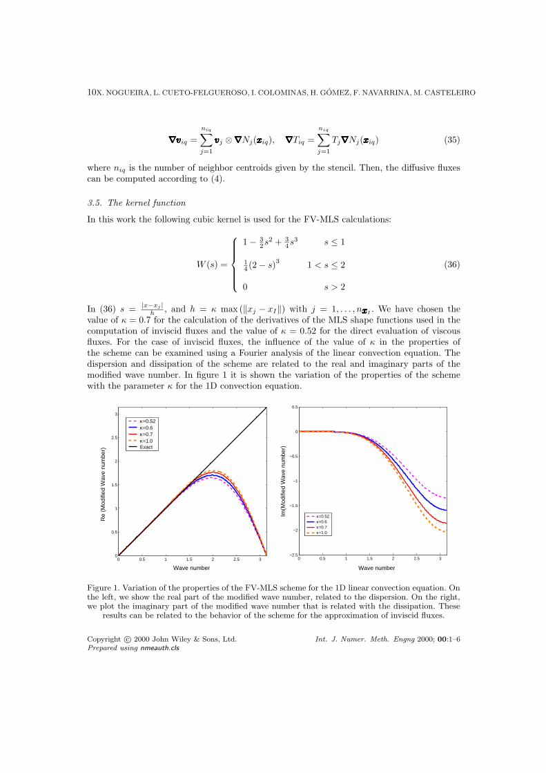
. We have chosen thevalue of κ = 0.7 for the calculation of the derivatives of the MLS shape functions used in thecomputation of inviscid fluxes and the value of κ = 0.52 for the direct evaluation of viscousfluxes. For the case of inviscid fluxes, the influence of the value of κ in the properties ofthe scheme can be examined using a Fourier analysis of the linear convection equation. Thedispersion and dissipation of the scheme are related to the real and imaginary parts of themodified wave number. In figure 1 it is shown the variation of the properties of the schemewith the parameter κ for the 1D convection equation.
0 0.5 1 1.5 2 2.5 30
0.5
1
1.5
2
2.5
3
Wave number
Re
(Mod
ified
Wav
e nu
mbe
r)
κ=0.52κ=0.6κ=0.7κ=1.0Exact
0 0.5 1 1.5 2 2.5 3−2.5
−2
−1.5
−1
−0.5
0
0.5
Im(M
odifi
ed W
ave
num
ber)
Wave number
κ=0.52κ=0.6κ=0.7κ=1.0
Figure 1. Variation of the properties of the FV-MLS scheme for the 1D linear convection equation. Onthe left, we show the real part of the modified wave number, related to the dispersion. On the right,we plot the imaginary part of the modified wave number that is related with the dissipation. These
results can be related to the behavior of the scheme for the approximation of inviscid fluxes.
Copyright c© 2000 John Wiley & Sons, Ltd. Int. J. Numer. Meth. Engng 2000; 00:1–6Prepared using nmeauth.cls
ON THE ACCURACY OF FV AND DG DISCRETIZATIONS FOR COMPRESSIBLE FLOW 11
For inviscid fluxes, the derivatives of the variables are used to compute a Taylorreconstruction of the variables inside the cell. For the direct evaluation of viscous fluxes orelliptic terms, the behavior is different, since the derivatives or variables that we compute areused directly. If we consider a 1D stencil, Fourier analysis gives the modified wave number forthe MLS approximation:
Modified Wave Number = MWN = (−i)Q∑
l=−P
∂Nlj
∂xeik(l∆x) (37)
where P is the number of neighbors to the left of the cell I and Q is the number of neighborsto the right of the cell I. Moreover, k is the wave number. In order to get some conclusions,we particularize for the case of a five-element stencil P = Q = 2:
MWN = (−i)Q∑
l=−P
∂Nlj
∂xeik(l∆x) =
= sin (2k∆x)(
∂N(I+2)
∂x− ∂N(I−2)
∂x
)+
sin (k∆x)(
∂N(I+1)
∂x− ∂N(I−1)
∂x
)− (38)
−i
(cos (2k∆x)
(∂N(I+2)
∂x+
∂N(I−2)
∂x
)+
+ cos (k∆x)(
∂N(I+1)
∂x+
∂N(I−1)
∂x
)+
∂NI
∂x
)
For an isotropic distribution of points and a given stencil for the cubic spline, there is noinfluence of the parameter κ on the real part of the MLS approximation, since the difference
of the shape functions∂N(I+i)
∂x− ∂N(I−i)
∂xis constant. Moreover
∂NI
∂x= 0 (39)
∂N(I+i)
∂x= −∂N(I−i)
∂x(40)
Then, the imaginary part of the approximation vanishes, and there is no dissipation. Weremark that this results only hold for the kernel (36). Even though for a given stencil themodified wave number is independent from κ, it affects the size of the support and thereforeit modifies the weighting of the points of the stencil, as we show on figure 2. Using radialweighting the support of the kernel expands over a circle of radius 2h, so it is worth to notethat the selection of a value of κ small could lead to a bad conditioning of the moment matrixMMMMMMMMMMMMMM . As a practical rule κ ≥ 0.52. In unstructured grids, the distribution of nodes is not isotropicand the behavior of the scheme will be affected. It is possible to define an optimum value ofκ for each point of the grid, and this subject is currently under research. On the other hand,it is clear than a different selection of the kernel function produce different properties of thescheme.
Copyright c© 2000 John Wiley & Sons, Ltd. Int. J. Numer. Meth. Engng 2000; 00:1–6Prepared using nmeauth.cls

12X. NOGUEIRA, L. CUETO-FELGUEROSO, I. COLOMINAS, H. GOMEZ, F. NAVARRINA, M. CASTELEIRO
−2 −1 0 1 20
0.1
0.2
0.3
0.4
0.5
0.6
0.7
0.8
0.9
1
x
Wκ=0.52κ=0.6 κ=0.7 κ=1.0
Figure 2. Variation of the shape of the cubic kernel in terms of κ. The kernel is centered in the cellI = 0. The distance between nodes is ∆x = 1.
3.5.1. Isotropic and non isotropic kernels. The most frequently used kernels in the literatureare splines and exponential functions. Kernels are defined over a support whose size iscontrolled by the smoothing length h. If the same smoothing length is used for each directionin a 2D problem, the support will be a circle with radius 2h. Another possibility would beto use different smoothing lengths for every direction. Then, if the kernel is defined as theproduct of the kernels in every direction, the support will be a rectangle (figure 3, left), butany other geometric form is possible (i.e. elliptical kernels). In addition, there is the possibilityof taking a kernel in the x direction different of the kernel taken for the y direction.
Figure 3. Support with different smoothing lengths (left) and orientation of inertial axis (right)
In order to build an anisotropic kernel we take the clouds of points given by the stencil andcalculate their principal inertial axis. Then we can obtain the direction of these axis (figure 3,right). In 2D, this is given by:
tan(2α) =2Ixy
Ixx − Iyy(41)
Copyright c© 2000 John Wiley & Sons, Ltd. Int. J. Numer. Meth. Engng 2000; 00:1–6Prepared using nmeauth.cls
ON THE ACCURACY OF FV AND DG DISCRETIZATIONS FOR COMPRESSIBLE FLOW 13
Then, changing the coordinates, with β = −α:
xxxxxxxxxxxxxx∗ =(
cos β − sinβsin β cosβ
)xxxxxxxxxxxxxx (42)
Now, we obtain the smoothing lengths in each new direction:
hx∗ = κx max (‖xj − xI‖) j = 1, . . . , nxxxxxxxxxxxxxxI
hy∗ = κy max (‖yj − yI‖) j = 1, . . . , nxxxxxxxxxxxxxxI(43)
and the rectangular anisotropic kernel will be given by:
W = Wx∗Wy∗ (44)
The derivatives in global coordinates are given by:
∂N∂x
∂N∂y
=
(cos β − sin βsin β cosβ
)
∂N∂x∗
∂N∂y∗
(45)
and the second derivatives by:
∂2N∂x2
∂2N∂x∂y
∂2N∂y∂x
∂2N∂y2
=
(cos β − sin βsin β cosβ
)
∂2N∂x∗2
∂2N∂x∗∂y∗
∂2N∂y∗∂x∗
∂2N∂y∗2
(cosβ − sin βsin β cos β
)
(46)Higher order derivatives are straightforward.
3.6. Full stencil of the MLS finite volume scheme
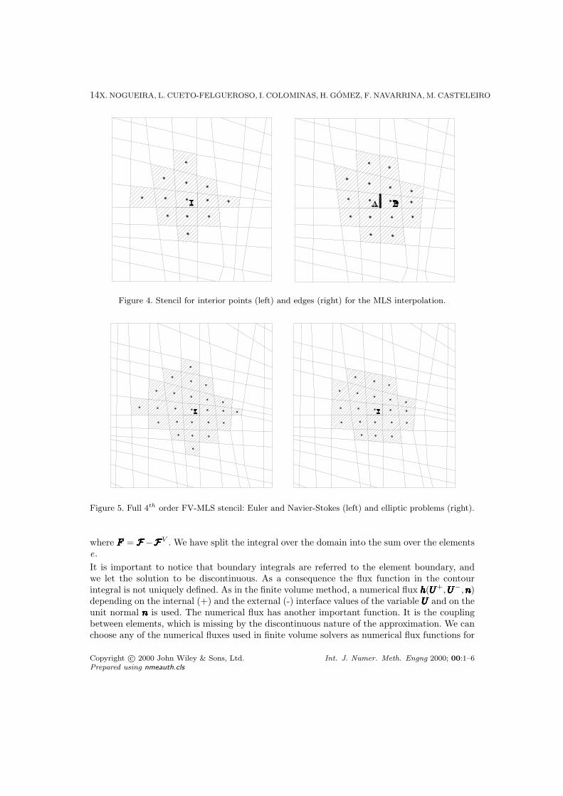
Figure 5 shows the stencils to compute the MLS shape functions for the fourth-order FV-MLSmethod. A complete description of the stencils can be found in [8, 9]. For inviscid problems,the stencil of a cell I is obtained as the union of its MLS stencil (figure 4)) and the MLSstencils of its first neighbors. As it can be seen in figure 5 the full stencil comprises 25 cells.Analogously, the stencil of the “viscous” discretization is obtained as the union of the MLSstencils associated to all the edges of cell I. This stencil comprises 21 cells.
4. DISCONTINUOUS GALERKIN METHODS
This section presents a brief introduction to discontinuous Galerkin (DG) methods forconvection-dominated problems. For a deeper insight, we refer the reader to [11, 13, 19, 20,21, 22] among others.
The weak form of (1) is:
∑e
[∫
Ωe
φ∂UUUUUUUUUUUUUUh
∂tdΩ−
∫
Ωe
∇∇∇∇∇∇∇∇∇∇∇∇∇∇φ ·FFFFFFFFFFFFFF (UUUUUUUUUUUUUU,∇∇∇∇∇∇∇∇∇∇∇∇∇∇UUUUUUUUUUUUUU)dΩ +∮
∂Ωe
φnnnnnnnnnnnnnn · FFFFFFFFFFFFFF (UUUUUUUUUUUUUU,∇∇∇∇∇∇∇∇∇∇∇∇∇∇UUUUUUUUUUUUUU)]
= 0, ∀φ (47)
Copyright c© 2000 John Wiley & Sons, Ltd. Int. J. Numer. Meth. Engng 2000; 00:1–6Prepared using nmeauth.cls
14X. NOGUEIRA, L. CUETO-FELGUEROSO, I. COLOMINAS, H. GOMEZ, F. NAVARRINA, M. CASTELEIRO
Figure 4. Stencil for interior points (left) and edges (right) for the MLS interpolation.
Figure 5. Full 4th order FV-MLS stencil: Euler and Navier-Stokes (left) and elliptic problems (right).
where FFFFFFFFFFFFFF = FFFFFFFFFFFFFF −FFFFFFFFFFFFFFV . We have split the integral over the domain into the sum over the elementse.It is important to notice that boundary integrals are referred to the element boundary, andwe let the solution to be discontinuous. As a consequence the flux function in the contourintegral is not uniquely defined. As in the finite volume method, a numerical flux hhhhhhhhhhhhhh(UUUUUUUUUUUUUU+,UUUUUUUUUUUUUU−, nnnnnnnnnnnnnn)depending on the internal (+) and the external (-) interface values of the variable UUUUUUUUUUUUUU and on theunit normal nnnnnnnnnnnnnn is used. The numerical flux has another important function. It is the couplingbetween elements, which is missing by the discontinuous nature of the approximation. We canchoose any of the numerical fluxes used in finite volume solvers as numerical flux functions for
Copyright c© 2000 John Wiley & Sons, Ltd. Int. J. Numer. Meth. Engng 2000; 00:1–6Prepared using nmeauth.cls
ON THE ACCURACY OF FV AND DG DISCRETIZATIONS FOR COMPRESSIBLE FLOW 15
the convective part. Here, we have chosen the same one as in the FV-MLS method. The problemappears in the definition of numerical fluxes for the viscous surface integrals. In this case, if weuse the common approach in finite volume schemes of central difference discretization for theevaluation of viscous fluxes, the solution seems to converge as we refine the mesh. However,it will be wrong and the error will have a component independent of grid size [19]. There aremany possibilities to deal with viscous fluxes in a Discontinuous Galerkin framework. Here,we will use the Local Discontinuous Galerkin (LDG) discretization [20].We transform the second order Navier-Stokes equations in a first order equivalent system.
SSSSSSSSSSSSSS = ∇∇∇∇∇∇∇∇∇∇∇∇∇∇UUUUUUUUUUUUUU (48)
∂UUUUUUUUUUUUUU
∂t+∇∇∇∇∇∇∇∇∇∇∇∇∇∇ · FFFFFFFFFFFFFF(UUUUUUUUUUUUUU)−∇∇∇∇∇∇∇∇∇∇∇∇∇∇ · FFFFFFFFFFFFFFV (UUUUUUUUUUUUUU,SSSSSSSSSSSSSS) = 0 (49)
We can write the weak form of both equations:∫
Ωe
SSSSSSSSSSSSSShφdΩe +∫
Ωe
UUUUUUUUUUUUUUh∇∇∇∇∇∇∇∇∇∇∇∇∇∇φ(u)dΩe −∮
Γe
UUUUUUUUUUUUUUh · nnnnnnnnnnnnnnφdσ = 0 (50)
∫
Ωe
φ∂UUUUUUUUUUUUUUh
∂tdΩe −
∫
Ωe
FFFFFFFFFFFFFF (UUUUUUUUUUUUUUh)∇∇∇∇∇∇∇∇∇∇∇∇∇∇φdΩe +∫
Ωe
FFFFFFFFFFFFFFV (UUUUUUUUUUUUUUh, SSSSSSSSSSSSSSh)∇∇∇∇∇∇∇∇∇∇∇∇∇∇φdΩe+∮
Γe
FFFFFFFFFFFFFF (UUUUUUUUUUUUUUh) · nnnnnnnnnnnnnnφdσ −∮
Γe
FFFFFFFFFFFFFFV (UUUUUUUUUUUUUUh, SSSSSSSSSSSSSSh) · nnnnnnnnnnnnnnφdσ = 0(51)
Following Arnold [21] we define on every interior edge the average q and the jump [q]operators as follows. Let e an interior edge shared by two elements Ω+
e and Ω−e . We definethe unit normal vectors nnnnnnnnnnnnnn+ and nnnnnnnnnnnnnn− on e pointing exterior to Ω+
e and Ω−e . Then, we set thefollowing:For q scalar:
q =12
(q+ + q−
)
[q] = q+nnnnnnnnnnnnnn+ + q−nnnnnnnnnnnnnn− (52)
For ϕϕϕϕϕϕϕϕϕϕϕϕϕϕ vector:
ϕϕϕϕϕϕϕϕϕϕϕϕϕϕ =12
(ϕϕϕϕϕϕϕϕϕϕϕϕϕϕ+ + ϕϕϕϕϕϕϕϕϕϕϕϕϕϕ−
)
[ϕϕϕϕϕϕϕϕϕϕϕϕϕϕ] = ϕϕϕϕϕϕϕϕϕϕϕϕϕϕ+ · nnnnnnnnnnnnnn+ + ϕϕϕϕϕϕϕϕϕϕϕϕϕϕ− · nnnnnnnnnnnnnn− (53)
For the first equation, the LDG scheme defines the following numerical flux. If the edge e isinside the domain Ω, then:
UUUUUUUUUUUUUUh · nnnnnnnnnnnnnn = (UUUUUUUUUUUUUU+ ββββββββββββββ · [UUUUUUUUUUUUUU ]) · nnnnnnnnnnnnnn (54)
and if e lies on the boundary of Ω:
UUUUUUUUUUUUUUh · nnnnnnnnnnnnnn =
ggggggggggggggD · nnnnnnnnnnnnnn on ΓD
UUUUUUUUUUUUUU+ · nnnnnnnnnnnnnn on ΓN(55)
where ΓD and ΓN are the Dirichlet and Neumann boundaries, and ggggggggggggggD is the value of UUUUUUUUUUUUUU on theDirichlet boundary.
Copyright c© 2000 John Wiley & Sons, Ltd. Int. J. Numer. Meth. Engng 2000; 00:1–6Prepared using nmeauth.cls
16X. NOGUEIRA, L. CUETO-FELGUEROSO, I. COLOMINAS, H. GOMEZ, F. NAVARRINA, M. CASTELEIRO
For the second equation the inviscid flux is one of the commonly used in finite volumemethod. Numerical viscous flux for the edges inside the domain is the following:
FFFFFFFFFFFFFFV · nnnnnnnnnnnnnn =(FFFFFFFFFFFFFFV
− ββββββββββββββ · [FFFFFFFFFFFFFFV]− α [UUUUUUUUUUUUUU ]
) · nnnnnnnnnnnnnn (56)
and for the boundaries:
FFFFFFFFFFFFFFV · nnnnnnnnnnnnnn =
(FVFVFVFVFVFVFVFVFVFVFVFVFVFV + − α
(UUUUUUUUUUUUUU+ − ggggggggggggggD
)nnnnnnnnnnnnnn)· nnnnnnnnnnnnnn on ΓD
ggggggggggggggN · nnnnnnnnnnnnnn on ΓN
(57)
where ggggggggggggggN is the value of FVFVFVFVFVFVFVFVFVFVFVFVFVFV on the Neumann boundary.Following [22] the value of α = 1 has been chosen, and the definition of ββββββββββββββ on each edge e is
as follows:ββββββββββββββ · nnnnnnnnnnnnnn = sign(vvvvvvvvvvvvvv · nnnnnnnnnnnnnn)/2 (58)
where vvvvvvvvvvvvvv is an arbitrary but fixed vector with nonzero components. This vector is taken asvvvvvvvvvvvvvv = (1, 1).
After assembling all the elemental contributions, the system can be written as:
MMMMMMMMMMMMMMdUUUUUUUUUUUUUUh
dt+ RRRRRRRRRRRRRR(UUUUUUUUUUUUUUh) = 0 (59)
where MMMMMMMMMMMMMM is the mass matrix and RRRRRRRRRRRRRR is the residual.
5. PIECEWISE POLYNOMIAL INTERPOLATION VS. MOVING LEAST SQUARES
Most of the existing high order schemes are based on piecewise polynomial interpolation.Following this approach, higher order accuracy is obtained by creating new degrees of freedominside each element/cell, which are used to construct an interpolating polynomial. From theperspective of pure interpolation, the reconstructed value at a point inside an element dependssolely on the variables at the nodes inside that element. It is clear that for points located atedges and corners of the element there is a bias in the direction of the incoming information,which necessarily has an impact on the global accuracy of the numerical scheme. Furthermore,even for moderately high order polynomial interpolations the Runge phenomenon preventsthe use of uniform nodal distributions. While an approximation that is discontinuous acrossinterfaces seems somewhat natural for hyperbolic problems, it is rather inconvenient for thediscretization of terms involving high order derivatives.
On the other hand, moving least squares (MLS) provide a general, pointwise centered,approximation framework, that may be used in order to construct both higher orderreconstructions in the sense of classical Godunov-type methods, and also accuratediscretizations of elliptic-like terms. It is interesting at this point to examine the relativeperformance of piecewise polynomial and MLS approximations. Firstly, this analysis willprovide some insight into the efficiency of the schemes, in terms of how much informationis extracted from a given grid. Secondly, the results of the present analysis may helpunderstanding, at least in part, the relative accuracy in the numerical solution of boundaryvalue problems achieved by techniques that use one method or the other.
An important remark is that, while one may construct polynomial expansions of arbitrarilyhigh orders (provided that a careful choice of expansion basis and collocation points is made),
Copyright c© 2000 John Wiley & Sons, Ltd. Int. J. Numer. Meth. Engng 2000; 00:1–6Prepared using nmeauth.cls
ON THE ACCURACY OF FV AND DG DISCRETIZATIONS FOR COMPRESSIBLE FLOW 17
Moving Least-Squares approximation are necessarily restricted to low or moderately high orderexpansions. We believe, however, that the attainable orders within the MLS context (up tofourth-sixth order) are high enough for practical unstructured-grid computations.
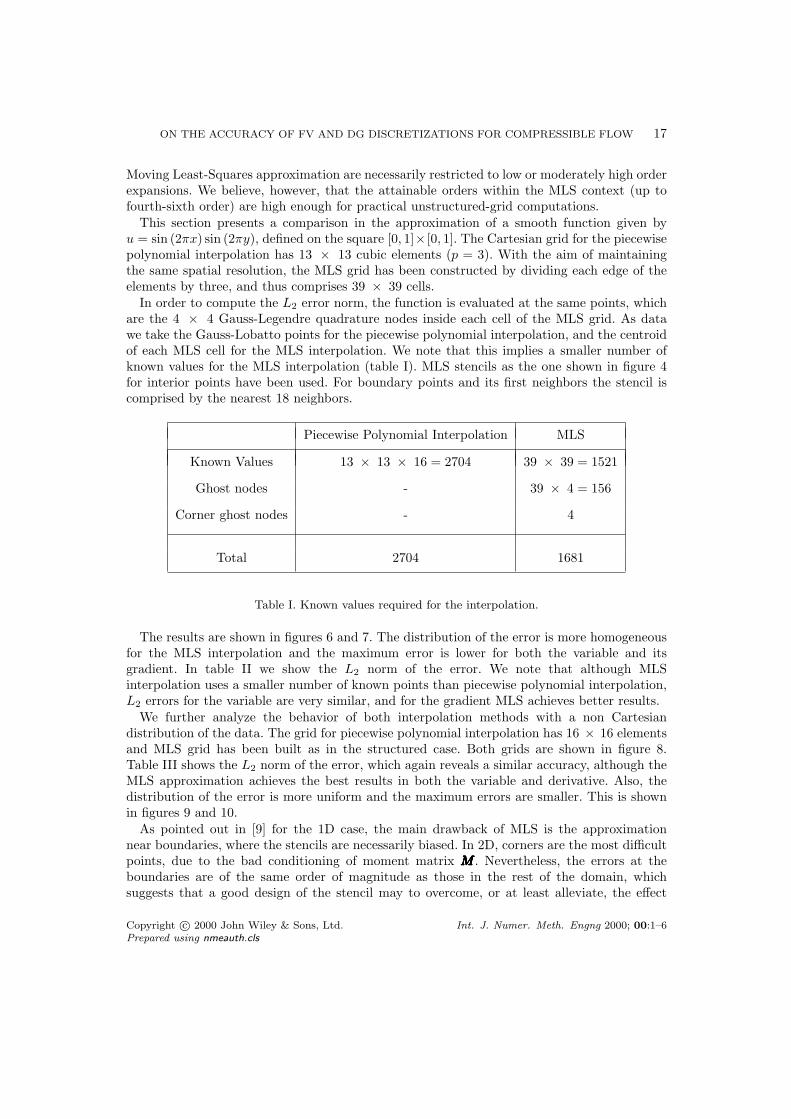
This section presents a comparison in the approximation of a smooth function given byu = sin (2πx) sin (2πy), defined on the square [0, 1]× [0, 1]. The Cartesian grid for the piecewisepolynomial interpolation has 13 × 13 cubic elements (p = 3). With the aim of maintainingthe same spatial resolution, the MLS grid has been constructed by dividing each edge of theelements by three, and thus comprises 39 × 39 cells.
In order to compute the L2 error norm, the function is evaluated at the same points, whichare the 4 × 4 Gauss-Legendre quadrature nodes inside each cell of the MLS grid. As datawe take the Gauss-Lobatto points for the piecewise polynomial interpolation, and the centroidof each MLS cell for the MLS interpolation. We note that this implies a smaller number ofknown values for the MLS interpolation (table I). MLS stencils as the one shown in figure 4for interior points have been used. For boundary points and its first neighbors the stencil iscomprised by the nearest 18 neighbors.
Piecewise Polynomial Interpolation MLS
Known Values 13 × 13 × 16 = 2704 39 × 39 = 1521
Ghost nodes - 39 × 4 = 156
Corner ghost nodes - 4
Total 2704 1681
Table I. Known values required for the interpolation.
The results are shown in figures 6 and 7. The distribution of the error is more homogeneousfor the MLS interpolation and the maximum error is lower for both the variable and itsgradient. In table II we show the L2 norm of the error. We note that although MLSinterpolation uses a smaller number of known points than piecewise polynomial interpolation,L2 errors for the variable are very similar, and for the gradient MLS achieves better results.
We further analyze the behavior of both interpolation methods with a non Cartesiandistribution of the data. The grid for piecewise polynomial interpolation has 16 × 16 elementsand MLS grid has been built as in the structured case. Both grids are shown in figure 8.Table III shows the L2 norm of the error, which again reveals a similar accuracy, although theMLS approximation achieves the best results in both the variable and derivative. Also, thedistribution of the error is more uniform and the maximum errors are smaller. This is shownin figures 9 and 10.
As pointed out in [9] for the 1D case, the main drawback of MLS is the approximationnear boundaries, where the stencils are necessarily biased. In 2D, corners are the most difficultpoints, due to the bad conditioning of moment matrix MMMMMMMMMMMMMM . Nevertheless, the errors at theboundaries are of the same order of magnitude as those in the rest of the domain, whichsuggests that a good design of the stencil may to overcome, or at least alleviate, the effect
Copyright c© 2000 John Wiley & Sons, Ltd. Int. J. Numer. Meth. Engng 2000; 00:1–6Prepared using nmeauth.cls

18X. NOGUEIRA, L. CUETO-FELGUEROSO, I. COLOMINAS, H. GOMEZ, F. NAVARRINA, M. CASTELEIRO
PiecewisePolynomial Interpolation MLS
U 1.28 E − 05 1.57 E − 05
∂U
∂x1.12 E − 03 8.31 E − 04
∂U
∂y1.12 E − 03 8.31 E − 04
∇∇∇∇∇∇∇∇∇∇∇∇∇∇U 1.58 E − 03 1.18 E − 03
Table II. L2 norm of the errors for the interpolation of u = sin (2πx) × sin (2πy) and its derivativeson a Cartesian grid.
Figure 6. Absolute value of the error for piecewise polynomial interpolation (A,C) and MLSinterpolation (B,D), for u = sin (2πx)× sin (2πy) on a Cartesian grid. A and B show a perspective of
the domain, C and D show a front view.
of boundaries. We believe that these better results of MLS in comparison with piecewisepolynomial interpolation are due to its local and centered characteristics. These featuresare specially appealing for non-regular point distributions. It is precisely in this kind ofenvironment where MLS more clearly outperforms piecewise polynomial interpolations. Also,the continuous nature of MLS interpolation across interfaces is a great advantage for thenumerical solution of elliptic terms.
Copyright c© 2000 John Wiley & Sons, Ltd. Int. J. Numer. Meth. Engng 2000; 00:1–6Prepared using nmeauth.cls
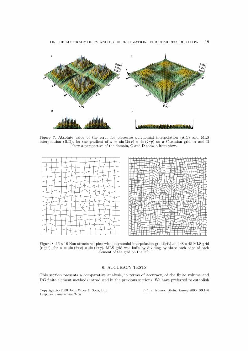
ON THE ACCURACY OF FV AND DG DISCRETIZATIONS FOR COMPRESSIBLE FLOW 19
Figure 7. Absolute value of the error for piecewise polynomial interpolation (A,C) and MLSinterpolation (B,D), for the gradient of u = sin (2πx) × sin (2πy) on a Cartesian grid. A and B
show a perspective of the domain, C and D show a front view.
Figure 8. 16× 16 Non-structured piecewise polynomial interpolation grid (left) and 48× 48 MLS grid(right), for u = sin (2πx) × sin (2πy). MLS grid was built by dividing by three each edge of each
element of the grid on the left.
6. ACCURACY TESTS
This section presents a comparative analysis, in terms of accuracy, of the finite volume andDG finite element methods introduced in the previous sections. We have preferred to establish
Copyright c© 2000 John Wiley & Sons, Ltd. Int. J. Numer. Meth. Engng 2000; 00:1–6Prepared using nmeauth.cls
20X. NOGUEIRA, L. CUETO-FELGUEROSO, I. COLOMINAS, H. GOMEZ, F. NAVARRINA, M. CASTELEIRO
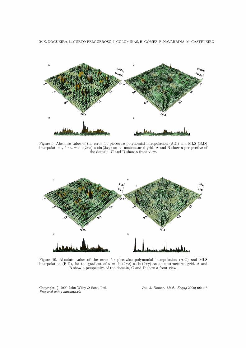
Figure 9. Absolute value of the error for piecewise polynomial interpolation (A,C) and MLS (B,D)interpolation , for u = sin (2πx) × sin (2πy) on an unstructured grid. A and B show a perspective of
the domain, C and D show a front view.
Figure 10. Absolute value of the error for piecewise polynomial interpolation (A,C) and MLSinterpolation (B,D), for the gradient of u = sin (2πx) × sin (2πy) on an unstructured grid. A and
B show a perspective of the domain, C and D show a front view.
Copyright c© 2000 John Wiley & Sons, Ltd. Int. J. Numer. Meth. Engng 2000; 00:1–6Prepared using nmeauth.cls
ON THE ACCURACY OF FV AND DG DISCRETIZATIONS FOR COMPRESSIBLE FLOW 21
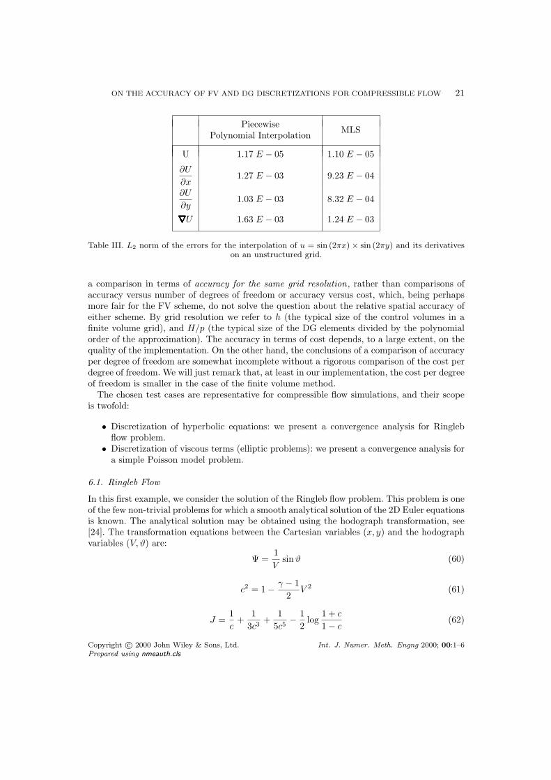
PiecewisePolynomial Interpolation MLS
U 1.17 E − 05 1.10 E − 05
∂U
∂x1.27 E − 03 9.23 E − 04
∂U
∂y1.03 E − 03 8.32 E − 04
∇∇∇∇∇∇∇∇∇∇∇∇∇∇U 1.63 E − 03 1.24 E − 03
Table III. L2 norm of the errors for the interpolation of u = sin (2πx) × sin (2πy) and its derivativeson an unstructured grid.
a comparison in terms of accuracy for the same grid resolution, rather than comparisons ofaccuracy versus number of degrees of freedom or accuracy versus cost, which, being perhapsmore fair for the FV scheme, do not solve the question about the relative spatial accuracy ofeither scheme. By grid resolution we refer to h (the typical size of the control volumes in afinite volume grid), and H/p (the typical size of the DG elements divided by the polynomialorder of the approximation). The accuracy in terms of cost depends, to a large extent, on thequality of the implementation. On the other hand, the conclusions of a comparison of accuracyper degree of freedom are somewhat incomplete without a rigorous comparison of the cost perdegree of freedom. We will just remark that, at least in our implementation, the cost per degreeof freedom is smaller in the case of the finite volume method.
The chosen test cases are representative for compressible flow simulations, and their scopeis twofold:
• Discretization of hyperbolic equations: we present a convergence analysis for Ringlebflow problem.
• Discretization of viscous terms (elliptic problems): we present a convergence analysis fora simple Poisson model problem.
6.1. Ringleb Flow
In this first example, we consider the solution of the Ringleb flow problem. This problem is oneof the few non-trivial problems for which a smooth analytical solution of the 2D Euler equationsis known. The analytical solution may be obtained using the hodograph transformation, see[24]. The transformation equations between the Cartesian variables (x, y) and the hodographvariables (V, ϑ) are:
Ψ =1V
sin ϑ (60)
c2 = 1− γ − 12
V 2 (61)
J =1c
+1
3c3+
15c5
− 12
log1 + c
1− c(62)
Copyright c© 2000 John Wiley & Sons, Ltd. Int. J. Numer. Meth. Engng 2000; 00:1–6Prepared using nmeauth.cls
22X. NOGUEIRA, L. CUETO-FELGUEROSO, I. COLOMINAS, H. GOMEZ, F. NAVARRINA, M. CASTELEIRO
ρ = c(
2γ − 1
)(63)
x =12ρ
[1
V 2− 2Ψ2
]+
J
2(64)
y = ± ΨρV
cos ϑ (65)
6.1.1. Problem setup. The computational domain is taken inside the regular Ringleb’sdomain. It is the rectangle [−1.15,−0.75] × [0.15, 0.55]. As boundary condition we set the(-) state of the flux function to be the exact one, as obtained through (60)–(65).
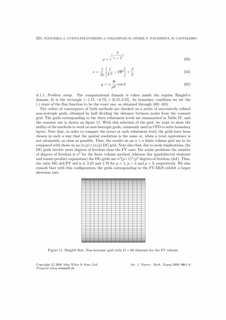
The orders of convergence of both methods are checked on a series of successively refinednon-isotropic grids, obtained by half dividing the distance between nodes from the coarsestgrid. The grids corresponding to the three refinement levels are summarized in Table IV, andthe coarsest one is shown on figure 11. With this selection of the grid, we want to show theability of the methods to work on non-isotropic grids, commonly used in CFD to solve boundarylayers. Note that, in order to compare the errors at each refinement level, the grids have beenchosen in such a way that the spatial resolution is the same or, when a total equivalence isnot attainable, as close as possible. Thus, the results on an n× n finite volume grid are to becompared with those on an (n/p)×(n/p) DG grid. Note also that, due to node duplications, theDG grids involve more degrees of freedom than the FV ones. For scalar problems the numberof degrees of freedom is n2 for the finite volume method, whereas (for quadrilateral elementsand tensor-product expansions) the DG grids use n2(p+1)2/p2 degrees of freedom (dof). Thus,the ratio DG dof/FV dof is 4, 2.25 and 1.78 for p = 1, p = 2 and p = 3, respectively. We alsoremark that with this configuration, the grids corresponding to the FV-MLS exhibit a largerskewness rate.
Figure 11. Ringleb flow. Non-isotropic grid with 15× 60 elements for the FV scheme.
Copyright c© 2000 John Wiley & Sons, Ltd. Int. J. Numer. Meth. Engng 2000; 00:1–6Prepared using nmeauth.cls
ON THE ACCURACY OF FV AND DG DISCRETIZATIONS FOR COMPRESSIBLE FLOW 23
FV-MLS DG
All orders p = 3 p = 2
15× 60 5× 20 8× 30
30× 120 10× 40 15× 60
60× 240 20× 60 30× 120
Table IV. Grids used for the Ringleb flow problem
We have used the non-isotropic formulation presented in section 3.5.1.
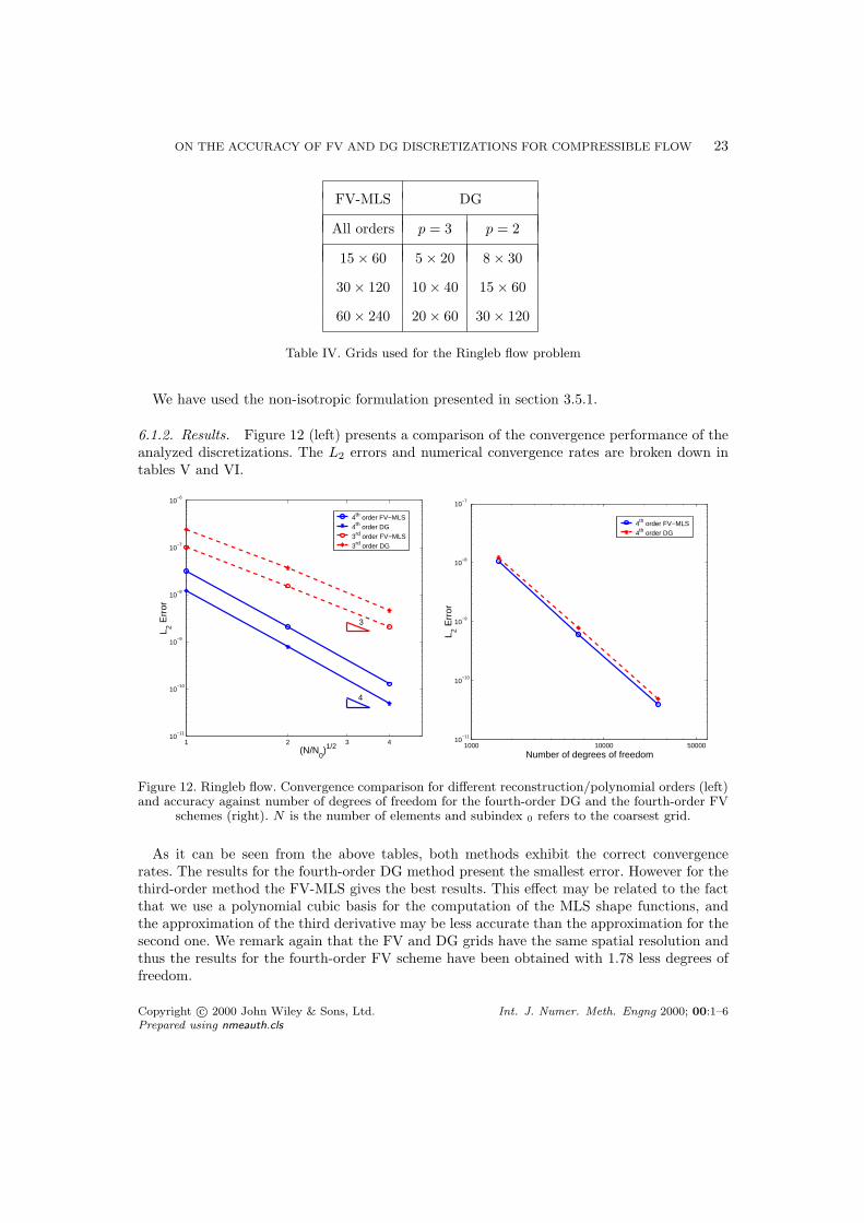
6.1.2. Results. Figure 12 (left) presents a comparison of the convergence performance of theanalyzed discretizations. The L2 errors and numerical convergence rates are broken down intables V and VI.
1 2 3 410
−11
10−10
10−9
10−8
10−7
10−6
(N/N0)1/2
L 2 Err
or
4th order FV−MLS4th order DG3rd order FV−MLS3rd order DG
3
4
1000 10000 5000010
−11
10−10
10−9
10−8
10−7
Number of degrees of freedom
L 2 Err
or
4th order FV−MLS4th order DG
Figure 12. Ringleb flow. Convergence comparison for different reconstruction/polynomial orders (left)and accuracy against number of degrees of freedom for the fourth-order DG and the fourth-order FV
schemes (right). N is the number of elements and subindex 0 refers to the coarsest grid.
As it can be seen from the above tables, both methods exhibit the correct convergencerates. The results for the fourth-order DG method present the smallest error. However for thethird-order method the FV-MLS gives the best results. This effect may be related to the factthat we use a polynomial cubic basis for the computation of the MLS shape functions, andthe approximation of the third derivative may be less accurate than the approximation for thesecond one. We remark again that the FV and DG grids have the same spatial resolution andthus the results for the fourth-order FV scheme have been obtained with 1.78 less degrees offreedom.
Copyright c© 2000 John Wiley & Sons, Ltd. Int. J. Numer. Meth. Engng 2000; 00:1–6Prepared using nmeauth.cls
24X. NOGUEIRA, L. CUETO-FELGUEROSO, I. COLOMINAS, H. GOMEZ, F. NAVARRINA, M. CASTELEIRO
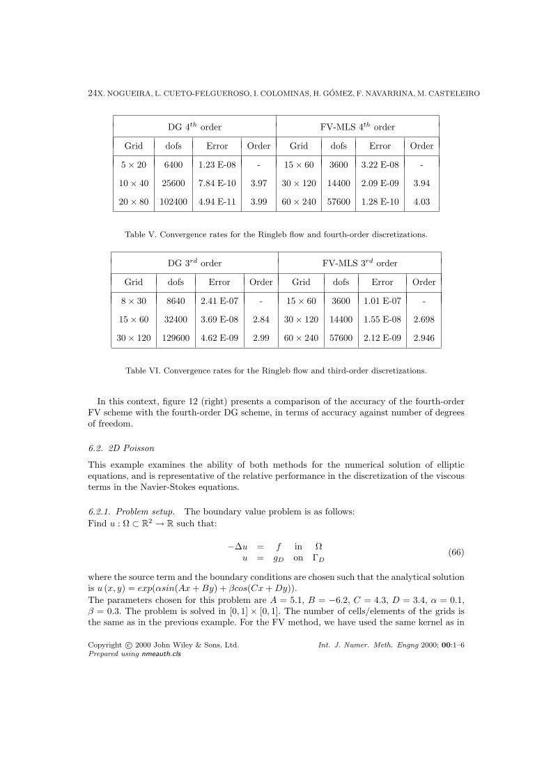
DG 4th order FV-MLS 4th order
Grid dofs Error Order Grid dofs Error Order
5× 20 6400 1.23 E-08 - 15× 60 3600 3.22 E-08 -
10× 40 25600 7.84 E-10 3.97 30× 120 14400 2.09 E-09 3.94
20× 80 102400 4.94 E-11 3.99 60× 240 57600 1.28 E-10 4.03
Table V. Convergence rates for the Ringleb flow and fourth-order discretizations.
DG 3rd order FV-MLS 3rd order
Grid dofs Error Order Grid dofs Error Order
8× 30 8640 2.41 E-07 - 15× 60 3600 1.01 E-07 -
15× 60 32400 3.69 E-08 2.84 30× 120 14400 1.55 E-08 2.698
30× 120 129600 4.62 E-09 2.99 60× 240 57600 2.12 E-09 2.946
Table VI. Convergence rates for the Ringleb flow and third-order discretizations.
In this context, figure 12 (right) presents a comparison of the accuracy of the fourth-orderFV scheme with the fourth-order DG scheme, in terms of accuracy against number of degreesof freedom.
6.2. 2D Poisson
This example examines the ability of both methods for the numerical solution of ellipticequations, and is representative of the relative performance in the discretization of the viscousterms in the Navier-Stokes equations.
6.2.1. Problem setup. The boundary value problem is as follows:Find u : Ω ⊂ R2 → R such that:
−∆u = f in Ωu = gD on ΓD
(66)
where the source term and the boundary conditions are chosen such that the analytical solutionis u (x, y) = exp(αsin(Ax + By) + βcos(Cx + Dy)).The parameters chosen for this problem are A = 5.1, B = −6.2, C = 4.3, D = 3.4, α = 0.1,β = 0.3. The problem is solved in [0, 1] × [0, 1]. The number of cells/elements of the grids isthe same as in the previous example. For the FV method, we have used the same kernel as in
Copyright c© 2000 John Wiley & Sons, Ltd. Int. J. Numer. Meth. Engng 2000; 00:1–6Prepared using nmeauth.cls
ON THE ACCURACY OF FV AND DG DISCRETIZATIONS FOR COMPRESSIBLE FLOW 25
the Ringleb flow problem. Note that, also in the FV scheme, the stencil is based on the celledges, since the gradients are computed directly at the quadrature points on the edges.
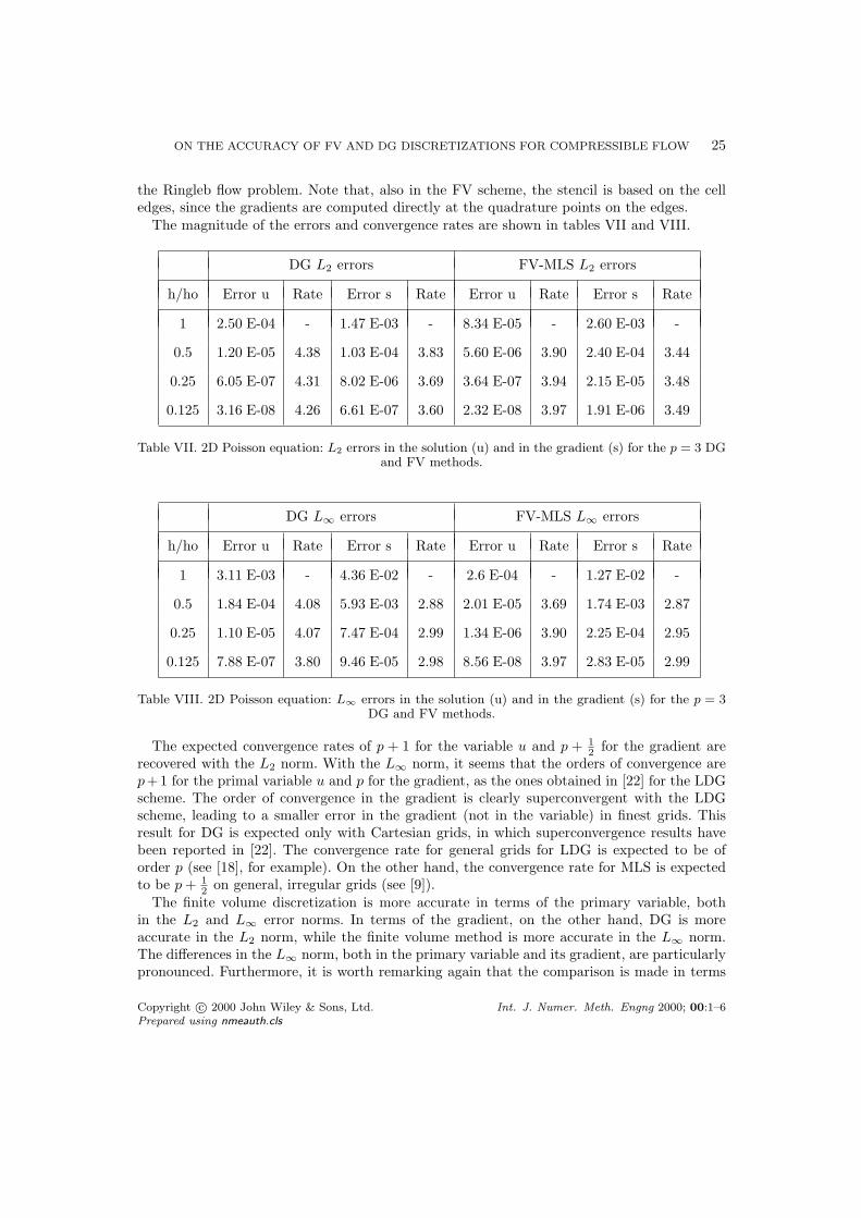
The magnitude of the errors and convergence rates are shown in tables VII and VIII.
DG L2 errors FV-MLS L2 errors
h/ho Error u Rate Error s Rate Error u Rate Error s Rate
1 2.50 E-04 - 1.47 E-03 - 8.34 E-05 - 2.60 E-03 -
0.5 1.20 E-05 4.38 1.03 E-04 3.83 5.60 E-06 3.90 2.40 E-04 3.44
0.25 6.05 E-07 4.31 8.02 E-06 3.69 3.64 E-07 3.94 2.15 E-05 3.48
0.125 3.16 E-08 4.26 6.61 E-07 3.60 2.32 E-08 3.97 1.91 E-06 3.49
Table VII. 2D Poisson equation: L2 errors in the solution (u) and in the gradient (s) for the p = 3 DGand FV methods.
DG L∞ errors FV-MLS L∞ errors
h/ho Error u Rate Error s Rate Error u Rate Error s Rate
1 3.11 E-03 - 4.36 E-02 - 2.6 E-04 - 1.27 E-02 -
0.5 1.84 E-04 4.08 5.93 E-03 2.88 2.01 E-05 3.69 1.74 E-03 2.87
0.25 1.10 E-05 4.07 7.47 E-04 2.99 1.34 E-06 3.90 2.25 E-04 2.95
0.125 7.88 E-07 3.80 9.46 E-05 2.98 8.56 E-08 3.97 2.83 E-05 2.99
Table VIII. 2D Poisson equation: L∞ errors in the solution (u) and in the gradient (s) for the p = 3DG and FV methods.
The expected convergence rates of p + 1 for the variable u and p + 12 for the gradient are
recovered with the L2 norm. With the L∞ norm, it seems that the orders of convergence arep+1 for the primal variable u and p for the gradient, as the ones obtained in [22] for the LDGscheme. The order of convergence in the gradient is clearly superconvergent with the LDGscheme, leading to a smaller error in the gradient (not in the variable) in finest grids. Thisresult for DG is expected only with Cartesian grids, in which superconvergence results havebeen reported in [22]. The convergence rate for general grids for LDG is expected to be oforder p (see [18], for example). On the other hand, the convergence rate for MLS is expectedto be p + 1
2 on general, irregular grids (see [9]).The finite volume discretization is more accurate in terms of the primary variable, both
in the L2 and L∞ error norms. In terms of the gradient, on the other hand, DG is moreaccurate in the L2 norm, while the finite volume method is more accurate in the L∞ norm.The differences in the L∞ norm, both in the primary variable and its gradient, are particularlypronounced. Furthermore, it is worth remarking again that the comparison is made in terms
Copyright c© 2000 John Wiley & Sons, Ltd. Int. J. Numer. Meth. Engng 2000; 00:1–6Prepared using nmeauth.cls
26X. NOGUEIRA, L. CUETO-FELGUEROSO, I. COLOMINAS, H. GOMEZ, F. NAVARRINA, M. CASTELEIRO
of grid resolution, and therefore the number of degrees of freedom is significantly higher in theDG case.
6.3. Summary and comments on the accuracy tests
As it has been seen, the FV-MLS results are comparable to the DG results, or even moreaccurate in both the inviscid and viscous test cases. We believe that this is due, at least inpart, to the nature of the interpolation process. In previous sections, it was explained thatMLS can be defined as a “centered” approximation whereas DG uses an interpolation that isbiased. It is clear that with MLS interpolation the information “comes” from all directions atevery cell (except for the boundary cells, which require ghost points). Another feature that mayhave an influence on the accuracy gap is the fact that the finite volume scheme is conservativeat a smaller scale than the DG scheme, which is also locally conservative but at the elementlevel . On the other hand, the straightforward discretization of the viscous fluxes is one of thegreatest advantages of the FV-MLS scheme for practical Navier-Stokes computations.
7. REPRESENTATIVE SIMULATIONS
In this section, our comparative analysis is extended to more practical unstructured-grid simulations. As in the previous cases, cubic polynomials for the DG case and cubicreconstruction for the FV-MLS method are used in order to obtain an equivalent order ofaccuracy.
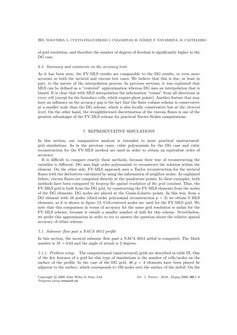
It is difficult to compare exactly these methods, because their way of reconstructing thevariables is different. DG uses high order polynomials to reconstruct the solution within theelement. On the other side, FV-MLS approach uses a Taylor reconstruction for the inviscidfluxes with the derivatives calculated by using the information of neighbor nodes. As explainedbefore, viscous fluxes are computed directly at the quadrature points. In these examples, bothmethods have been compared by keeping the spatial resolution of the grid constant. Thus, theFV-MLS grid is built from the DG grid, by constructing the FV-MLS elements from the nodesof the DG elements. DG nodes are placed at the Gauss-Lobatto points. In this way, from aDG element with 16 nodes (third-order polynomial reconstruction p = 3) we obtain 9 MLSelements, as it is shown in figure 13. Cell-centered nodes are used for the FV-MLS grid. Wenote that this comparison in terms of accuracy for the same grid resolution is unfair for theFV-MLS scheme, because it entails a smaller number of dofs for this scheme. Nevertheless,we prefer this approximation in order to try to answer the question about the relative spatialaccuracy of either scheme.
7.1. Subsonic flow past a NACA 0012 profile
In this section, the inviscid subsonic flow past a NACA 0012 airfoil is computed. The Machnumber is M = 0.63 and the angle of attack is 2 degrees.
7.1.1. Problem setup. The computational (unstructured) grids are described in table IX. Oneof the key features of a grid for this type of simulations is the number of cells/nodes on thesurface of the profile. In the case of the DG grid, 48 p = 3 elements have been placed lieadjacent to the surface, which corresponds to 192 nodes over the surface of the airfoil. On the
Copyright c© 2000 John Wiley & Sons, Ltd. Int. J. Numer. Meth. Engng 2000; 00:1–6Prepared using nmeauth.cls
ON THE ACCURACY OF FV AND DG DISCRETIZATIONS FOR COMPRESSIBLE FLOW 27
Figure 13. DG nodes (o) at Gauss-Lobatto points and FV-MLS elements from a single DG element.
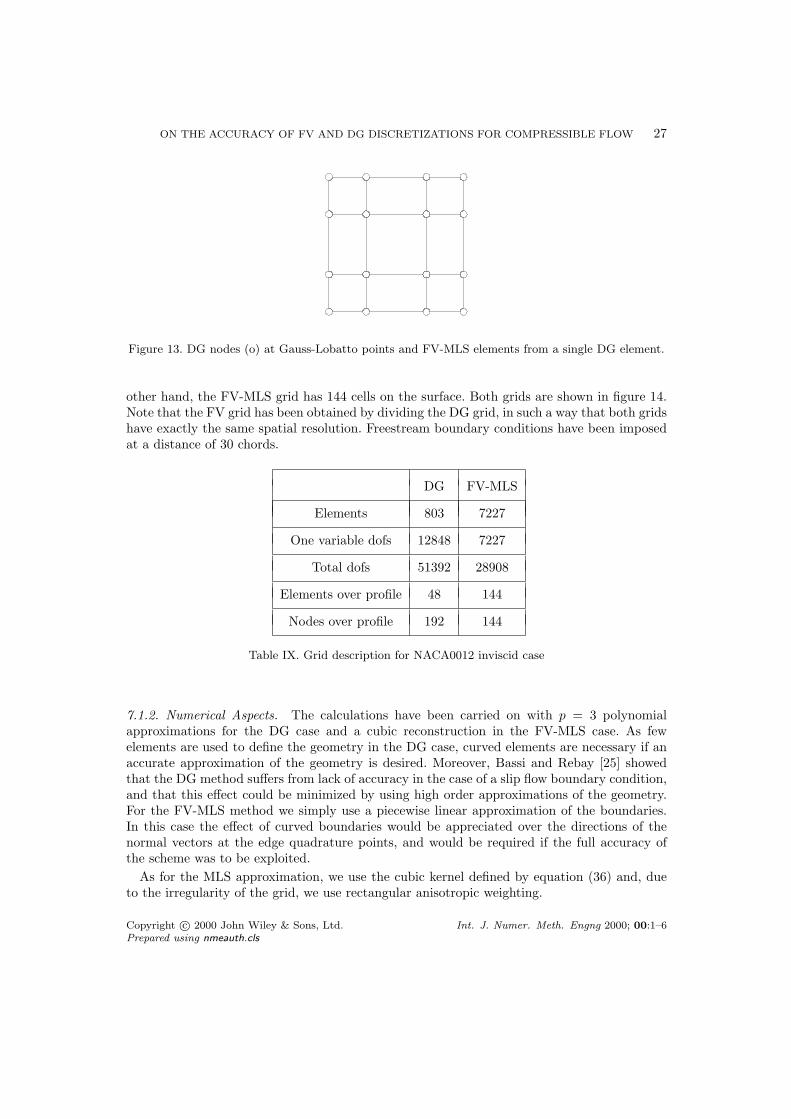
other hand, the FV-MLS grid has 144 cells on the surface. Both grids are shown in figure 14.Note that the FV grid has been obtained by dividing the DG grid, in such a way that both gridshave exactly the same spatial resolution. Freestream boundary conditions have been imposedat a distance of 30 chords.
DG FV-MLS
Elements 803 7227
One variable dofs 12848 7227
Total dofs 51392 28908
Elements over profile 48 144
Nodes over profile 192 144
Table IX. Grid description for NACA0012 inviscid case
7.1.2. Numerical Aspects. The calculations have been carried on with p = 3 polynomialapproximations for the DG case and a cubic reconstruction in the FV-MLS case. As fewelements are used to define the geometry in the DG case, curved elements are necessary if anaccurate approximation of the geometry is desired. Moreover, Bassi and Rebay [25] showedthat the DG method suffers from lack of accuracy in the case of a slip flow boundary condition,and that this effect could be minimized by using high order approximations of the geometry.For the FV-MLS method we simply use a piecewise linear approximation of the boundaries.In this case the effect of curved boundaries would be appreciated over the directions of thenormal vectors at the edge quadrature points, and would be required if the full accuracy ofthe scheme was to be exploited.
As for the MLS approximation, we use the cubic kernel defined by equation (36) and, dueto the irregularity of the grid, we use rectangular anisotropic weighting.
Copyright c© 2000 John Wiley & Sons, Ltd. Int. J. Numer. Meth. Engng 2000; 00:1–6Prepared using nmeauth.cls
28X. NOGUEIRA, L. CUETO-FELGUEROSO, I. COLOMINAS, H. GOMEZ, F. NAVARRINA, M. CASTELEIRO
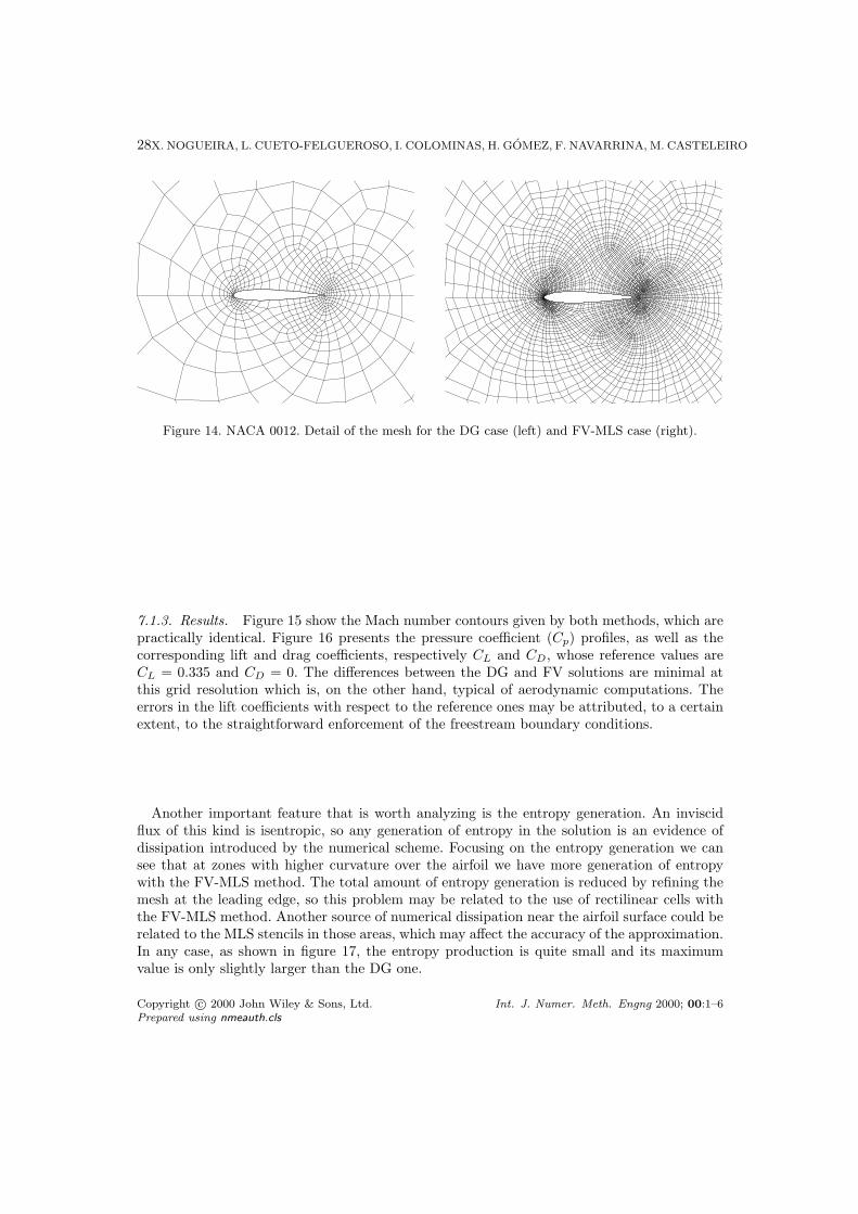
Figure 14. NACA 0012. Detail of the mesh for the DG case (left) and FV-MLS case (right).
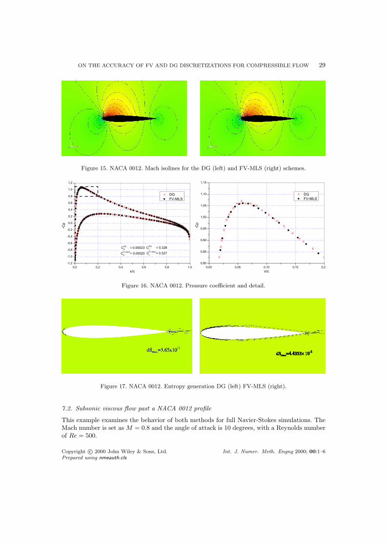
7.1.3. Results. Figure 15 show the Mach number contours given by both methods, which arepractically identical. Figure 16 presents the pressure coefficient (Cp) profiles, as well as thecorresponding lift and drag coefficients, respectively CL and CD, whose reference values areCL = 0.335 and CD = 0. The differences between the DG and FV solutions are minimal atthis grid resolution which is, on the other hand, typical of aerodynamic computations. Theerrors in the lift coefficients with respect to the reference ones may be attributed, to a certainextent, to the straightforward enforcement of the freestream boundary conditions.
Another important feature that is worth analyzing is the entropy generation. An inviscidflux of this kind is isentropic, so any generation of entropy in the solution is an evidence ofdissipation introduced by the numerical scheme. Focusing on the entropy generation we cansee that at zones with higher curvature over the airfoil we have more generation of entropywith the FV-MLS method. The total amount of entropy generation is reduced by refining themesh at the leading edge, so this problem may be related to the use of rectilinear cells withthe FV-MLS method. Another source of numerical dissipation near the airfoil surface could berelated to the MLS stencils in those areas, which may affect the accuracy of the approximation.In any case, as shown in figure 17, the entropy production is quite small and its maximumvalue is only slightly larger than the DG one.
Copyright c© 2000 John Wiley & Sons, Ltd. Int. J. Numer. Meth. Engng 2000; 00:1–6Prepared using nmeauth.cls
ON THE ACCURACY OF FV AND DG DISCRETIZATIONS FOR COMPRESSIBLE FLOW 29
Figure 15. NACA 0012. Mach isolines for the DG (left) and FV-MLS (right) schemes.
Figure 16. NACA 0012. Pressure coefficient and detail.
Figure 17. NACA 0012. Entropy generation DG (left) FV-MLS (right).
7.2. Subsonic viscous flow past a NACA 0012 profile
This example examines the behavior of both methods for full Navier-Stokes simulations. TheMach number is set as M = 0.8 and the angle of attack is 10 degrees, with a Reynolds numberof Re = 500.
Copyright c© 2000 John Wiley & Sons, Ltd. Int. J. Numer. Meth. Engng 2000; 00:1–6Prepared using nmeauth.cls
30X. NOGUEIRA, L. CUETO-FELGUEROSO, I. COLOMINAS, H. GOMEZ, F. NAVARRINA, M. CASTELEIRO
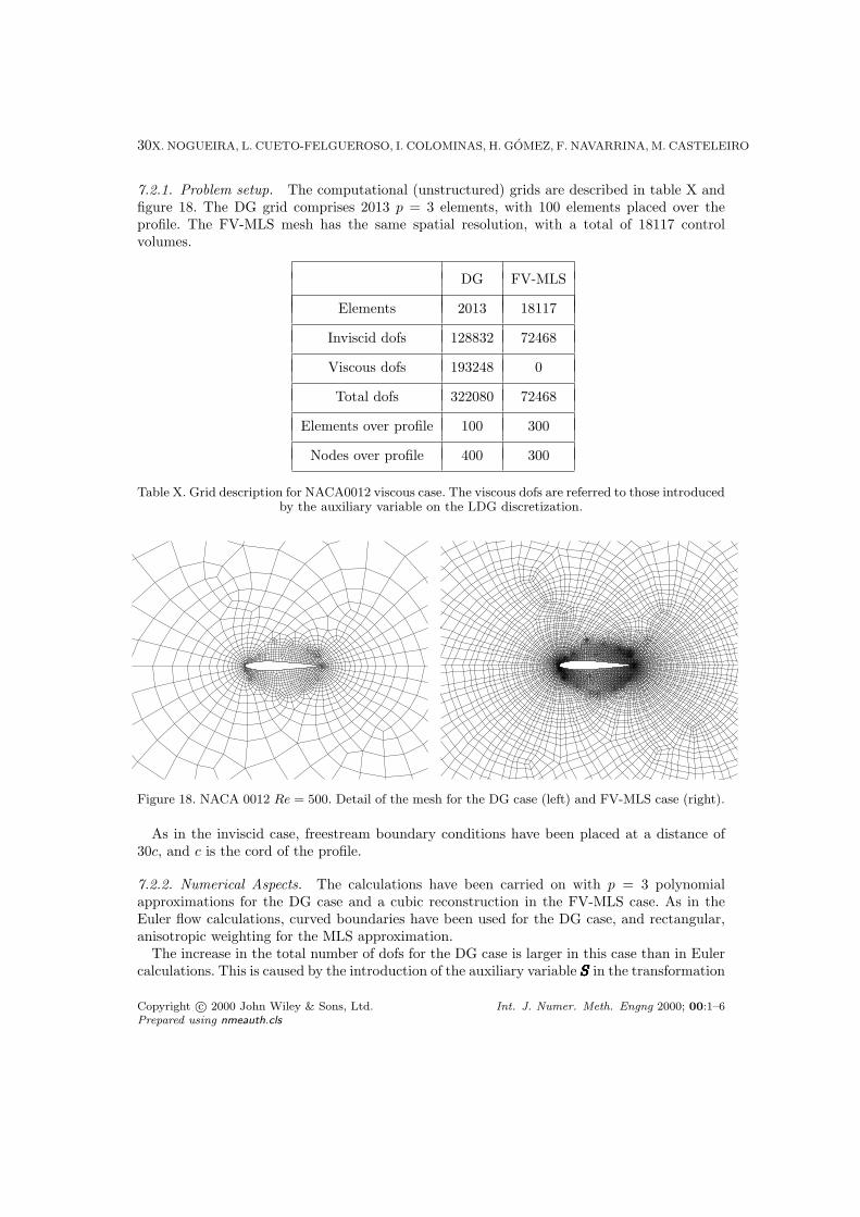
7.2.1. Problem setup. The computational (unstructured) grids are described in table X andfigure 18. The DG grid comprises 2013 p = 3 elements, with 100 elements placed over theprofile. The FV-MLS mesh has the same spatial resolution, with a total of 18117 controlvolumes.
DG FV-MLS
Elements 2013 18117
Inviscid dofs 128832 72468
Viscous dofs 193248 0
Total dofs 322080 72468
Elements over profile 100 300
Nodes over profile 400 300
Table X. Grid description for NACA0012 viscous case. The viscous dofs are referred to those introducedby the auxiliary variable on the LDG discretization.
Figure 18. NACA 0012 Re = 500. Detail of the mesh for the DG case (left) and FV-MLS case (right).
As in the inviscid case, freestream boundary conditions have been placed at a distance of30c, and c is the cord of the profile.
7.2.2. Numerical Aspects. The calculations have been carried on with p = 3 polynomialapproximations for the DG case and a cubic reconstruction in the FV-MLS case. As in theEuler flow calculations, curved boundaries have been used for the DG case, and rectangular,anisotropic weighting for the MLS approximation.
The increase in the total number of dofs for the DG case is larger in this case than in Eulercalculations. This is caused by the introduction of the auxiliary variable SSSSSSSSSSSSSS in the transformation
Copyright c© 2000 John Wiley & Sons, Ltd. Int. J. Numer. Meth. Engng 2000; 00:1–6Prepared using nmeauth.cls
ON THE ACCURACY OF FV AND DG DISCRETIZATIONS FOR COMPRESSIBLE FLOW 31
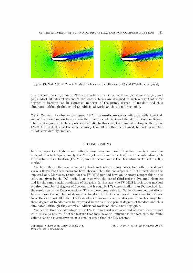
Figure 19. NACA 0012 Re = 500. Mach isolines for the DG case (left) and FV-MLS case (right).
of the second order system of PDE’s into a first order equivalent one (see equations (48) and(49)). Most DG discretizations of the viscous terms are designed in such a way that thesedegrees of freedom can be expressed in terms of the primal degrees of freedom and thuseliminated, although they entail an additional workload that is not negligible.
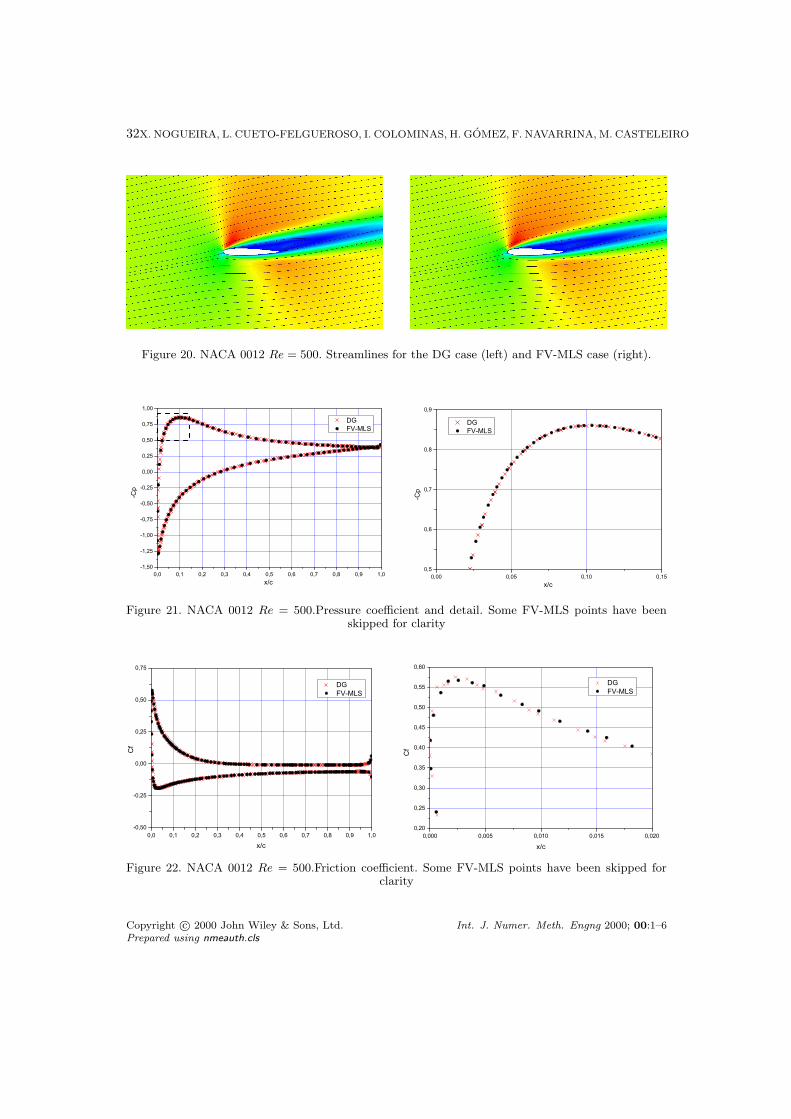
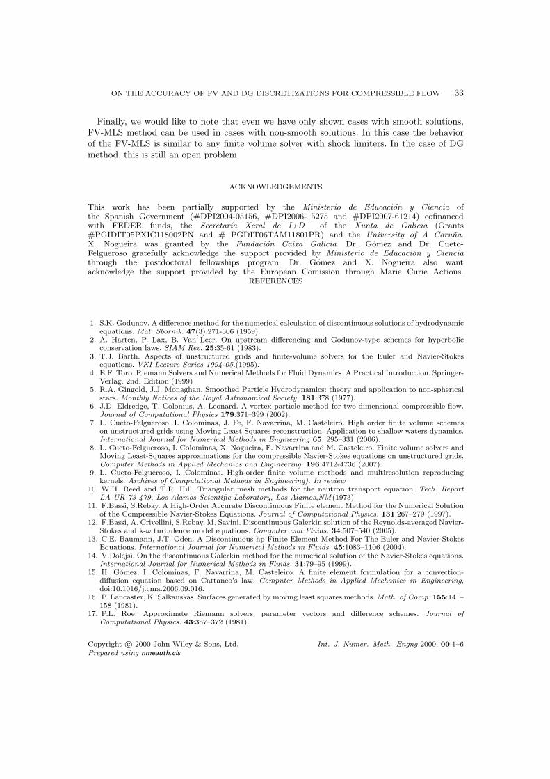
7.2.3. Results. As observed in figures 19-22, the results are very similar, virtually identical.As control variables, we have chosen the pressure coefficient and the skin friction coefficient.The results agree with those published in [26]. In this case, the main advantage of the use ofFV-MLS is that at least the same accuracy than DG method is obtained, but with a numberof dofs considerably smaller.
8. CONCLUSIONS
In this paper two high order methods have been compared. The first one is a meshfreeinterpolation technique (namely, the Moving Least-Squares method) used in combination withfinite volume discretization (FV-MLS) and the second one is the Discontinuous Galerkin (DG)method.
We have shown the results given by both methods in many cases, for both inviscid andviscous flows. For these cases we have checked that the convergence of both methods is theexpected one. Moreover, results for the FV-MLS method have an accuracy comparable to thesolutions given by the DG method, at least with the use of third-order polynomial elementsand for the same spatial resolution of the grids. In this case, the FV-MLS fourth-order methodrequires a number of degrees of freedom that is roughly 1.78 times smaller than DG method, forthe resolution of the Euler equations. This is more remarkable for Navier-Stokes computations.In this case, the number of degrees of freedom for DG is increased more than four times.Nevertheless, most DG discretizations of the viscous terms are designed in such a way thatthese degrees of freedom can be expressed in terms of the primal degrees of freedom and thuseliminated, although they entail an additional workload that is not negligible.
We believe that one advantage of the FV-MLS method is its local and centered features andits continuous nature. Another feature that may have an influence is the fact that the finitevolume scheme is conservative at a smaller scale than the DG scheme.
Copyright c© 2000 John Wiley & Sons, Ltd. Int. J. Numer. Meth. Engng 2000; 00:1–6Prepared using nmeauth.cls
32X. NOGUEIRA, L. CUETO-FELGUEROSO, I. COLOMINAS, H. GOMEZ, F. NAVARRINA, M. CASTELEIRO
Figure 20. NACA 0012 Re = 500. Streamlines for the DG case (left) and FV-MLS case (right).
0,0 0,1 0,2 0,3 0,4 0,5 0,6 0,7 0,8 0,9 1,0-1,50
-1,25
-1,00
-0,75
-0,50
-0,25
0,00
0,25
0,50
0,75
1,00
-Cp
x/c
DG FV-MLS
Figure 21. NACA 0012 Re = 500.Pressure coefficient and detail. Some FV-MLS points have beenskipped for clarity
0,0 0,1 0,2 0,3 0,4 0,5 0,6 0,7 0,8 0,9 1,0-0,50
-0,25
0,00
0,25
0,50
0,75
Cf
x/c
DG FV-MLS
0,000 0,005 0,010 0,015 0,0200,20
0,25
0,30
0,35
0,40
0,45
0,50
0,55
0,60
Cf
x/c
DG FV-MLS
Figure 22. NACA 0012 Re = 500.Friction coefficient. Some FV-MLS points have been skipped forclarity
Copyright c© 2000 John Wiley & Sons, Ltd. Int. J. Numer. Meth. Engng 2000; 00:1–6Prepared using nmeauth.cls
ON THE ACCURACY OF FV AND DG DISCRETIZATIONS FOR COMPRESSIBLE FLOW 33
Finally, we would like to note that even we have only shown cases with smooth solutions,FV-MLS method can be used in cases with non-smooth solutions. In this case the behaviorof the FV-MLS is similar to any finite volume solver with shock limiters. In the case of DGmethod, this is still an open problem.
ACKNOWLEDGEMENTS
This work has been partially supported by the Ministerio de Educacion y Ciencia ofthe Spanish Government (#DPI2004-05156, #DPI2006-15275 and #DPI2007-61214) cofinancedwith FEDER funds, the Secretarıa Xeral de I+D of the Xunta de Galicia (Grants#PGIDIT05PXIC118002PN and # PGDIT06TAM11801PR) and the University of A Coruna.X. Nogueira was granted by the Fundacion Caixa Galicia. Dr. Gomez and Dr. Cueto-Felgueroso gratefully acknowledge the support provided by Ministerio de Educacion y Cienciathrough the postdoctoral fellowships program. Dr. Gomez and X. Nogueira also wantacknowledge the support provided by the European Comission through Marie Curie Actions.
REFERENCES
1. S.K. Godunov. A difference method for the numerical calculation of discontinuous solutions of hydrodynamicequations. Mat. Sbornik. 47(3):271-306 (1959).
2. A. Harten, P. Lax, B. Van Leer. On upstream differencing and Godunov-type schemes for hyperbolicconservation laws. SIAM Rev. 25:35-61 (1983).
3. T.J. Barth. Aspects of unstructured grids and finite-volume solvers for the Euler and Navier-Stokesequations. VKI Lecture Series 1994-05.(1995).
4. E.F. Toro. Riemann Solvers and Numerical Methods for Fluid Dynamics. A Practical Introduction. Springer-Verlag. 2nd. Edition.(1999)
5. R.A. Gingold, J.J. Monaghan. Smoothed Particle Hydrodynamics: theory and application to non-sphericalstars. Monthly Notices of the Royal Astronomical Society. 181:378 (1977).
6. J.D. Eldredge, T. Colonius, A. Leonard. A vortex particle method for two-dimensional compressible flow.Journal of Computational Physics 179:371–399 (2002).
7. L. Cueto-Felgueroso, I. Colominas, J. Fe, F. Navarrina, M. Casteleiro. High order finite volume schemeson unstructured grids using Moving Least Squares reconstruction. Application to shallow waters dynamics.International Journal for Numerical Methods in Engineering 65: 295–331 (2006).
8. L. Cueto-Felgueroso, I. Colominas, X. Nogueira, F. Navarrina and M. Casteleiro. Finite volume solvers andMoving Least-Squares approximations for the compressible Navier-Stokes equations on unstructured grids.Computer Methods in Applied Mechanics and Engineering. 196:4712-4736 (2007).
9. L. Cueto-Felgueroso, I. Colominas. High-order finite volume methods and multiresolution reproducingkernels. Archives of Computational Methods in Engineering). In review
10. W.H. Reed and T.R. Hill. Triangular mesh methods for the neutron transport equation. Tech. ReportLA-UR-73-479, Los Alamos Scientific Laboratory, Los Alamos,NM (1973)
11. F.Bassi, S.Rebay. A High-Order Accurate Discontinuous Finite element Method for the Numerical Solutionof the Compressible Navier-Stokes Equations. Journal of Computational Physics. 131:267–279 (1997).
12. F.Bassi, A. Crivellini, S.Rebay, M. Savini. Discontinuous Galerkin solution of the Reynolds-averaged Navier-Stokes and k-ω turbulence model equations. Computer and Fluids. 34:507–540 (2005).
13. C.E. Baumann, J.T. Oden. A Discontinuous hp Finite Element Method For The Euler and Navier-StokesEquations. International Journal for Numerical Methods in Fluids. 45:1083–1106 (2004).
14. V.Dolejsi. On the discontinuous Galerkin method for the numerical solution of the Navier-Stokes equations.International Journal for Numerical Methods in Fluids. 31:79–95 (1999).
15. H. Gomez, I. Colominas, F. Navarrina, M. Casteleiro. A finite element formulation for a convection-diffusion equation based on Cattaneo’s law. Computer Methods in Applied Mechanics in Engineering,doi:10.1016/j.cma.2006.09.016.
16. P. Lancaster, K. Salkauskas. Surfaces generated by moving least squares methods. Math. of Comp. 155:141–158 (1981).
17. P.L. Roe. Approximate Riemann solvers, parameter vectors and difference schemes. Journal ofComputational Physics. 43:357–372 (1981).
Copyright c© 2000 John Wiley & Sons, Ltd. Int. J. Numer. Meth. Engng 2000; 00:1–6Prepared using nmeauth.cls

34X. NOGUEIRA, L. CUETO-FELGUEROSO, I. COLOMINAS, H. GOMEZ, F. NAVARRINA, M. CASTELEIRO
18. P.Persson and J.Peraire. An efficient low memory implicit DG algorithm for time dependent problems. 44thAIAA Aerospace Sciences Meeting, AIAA-2006-0113, Reno, Nevada, 2006.
19. M. Zhang, C.-W. Shu. An analysis of three different formulations of the Discontinuous Galerkin methodfor diffusion equations. Mathematical Models and Methods in Applied Sciences 13(3):395–413 (2003).
20. B. Cockburn,C.-W. Shu. The local discontinuous Galerkin finite element method for convection-diffusionsystems. SIAM Journal on Numerical Analysis 35:2440–2463 (1998).
21. D.N. Arnold, F. Brezzi, B. Cockburn, D. Marini. Unified analysis of Discontinuous Galerkin Methods forelliptic problems. SIAM Journal on Numerical Analysis 39(5):1749–1779 (1998).
22. B. Cockburn, G. Kanschat, I. Perugia, D. Schtzau. Superconvergence of the Local Discontinuous Galerkinmethod for elliptic problems on cartesian grids. SIAM Journal of Numerical Analysis. 39(1):264-285 (2001).
23. A. Crivellini, F. Bassi A three-dimensional parallel discontinuous Galerkin solver for acoustic propagationstudies. International Journal of aeroacoustics. Volume 2 2:157-174 (2003).
24. G. Chiocchia. Exact solutions to transonic and supersonic flows. Technical Report AR-211, AGARD, 1985.25. F. Bassi and S. Rebay. High-order accurate discontinuous finite element solution of the 2D Euler equations.
Journal of Computational Physics. 138:251-285 (1997).26. M.O, Bristeau, R. Glowinski, J. Periaux, H. Viviand (Eds). Numerical simulation of compressible Navier-
Stokes flows. Notes on Numerical Fluids Mechanics. Volume 18 2:(1987).
Copyright c© 2000 John Wiley & Sons, Ltd. Int. J. Numer. Meth. Engng 2000; 00:1–6Prepared using nmeauth.cls