oncomputingtheforcesfromthenoisydisplacementdata ...suresh/journal/j49ijnmereddy.pdf · int. j....

INTERNATIONAL JOURNAL FOR NUMERICAL METHODS IN ENGINEERINGInt. J. Numer. Meth. Engng 2008; 76:1645–1677Published online 22 July 2008 in Wiley InterScience (www.interscience.wiley.com). DOI: 10.1002/nme.2373

On computing the forces from the noisy displacement dataof an elastic body

A. Narayana Reddy and G. K. Ananthasuresh∗,†

Department of Mechanical Engineering, Indian Institute of Science, Bangalore, Karnataka, India

SUMMARY

This study is concerned with the accurate computation of the unknown forces applied on the boundary ofan elastic body using its measured displacement data with noise. Vision-based minimally intrusive force-sensing using elastically deformable grasping tools is the motivation for undertaking this problem. Since thisproblem involves incomplete and inconsistent displacement/force of an elastic body, it leads to an ill-posedproblem known as Cauchy’s problem in elasticity. Vision-based displacement measurement necessitateslarge displacements of the elastic body for reasonable accuracy. Therefore, we use geometrically non-linearmodelling of the elastic body, which was not considered by others who attempted to solve Cauchy’selasticity problem before. We present two methods to solve the problem. The first method uses thepseudo-inverse of an over-constrained system of equations. This method is shown to be not effectivewhen the noise in the measured displacement data is high. We attribute this to the appearance of spuriousforces at regions where there should not be any forces. The second method focuses on minimizing thespurious forces by varying the measured displacements within the known accuracy of the measurementtechnique. Both continuum and frame elements are used in the finite element modelling of the elasticbodies considered in the numerical examples. The performance of the two methods is compared usingseven numerical examples, all of which show that the second method estimates the forces with an errorthat is not more than the noise in the measured displacements. An experiment was also conducted todemonstrate the effectiveness of the second method in accurately estimating the applied forces. Copyrightq 2008 John Wiley & Sons, Ltd.

Received 19 October 2007; Revised 14 February 2008; Accepted 27 March 2008

KEY WORDS: vision-based force sensor; geometric non-linearity; inverse problems; Cauchy’s problem

∗Correspondence to: G. K. Ananthasuresh, Department of Mechanical Engineering, Indian Institute of Science,Bangalore, Karnataka, India.

†E-mail: [email protected]

Contract/grant sponsor: Department of Science and Technology, Government of India

Copyright q 2008 John Wiley & Sons, Ltd.

1646 A. N. REDDY AND G. K. ANANTHASURESH

1. INTRODUCTION

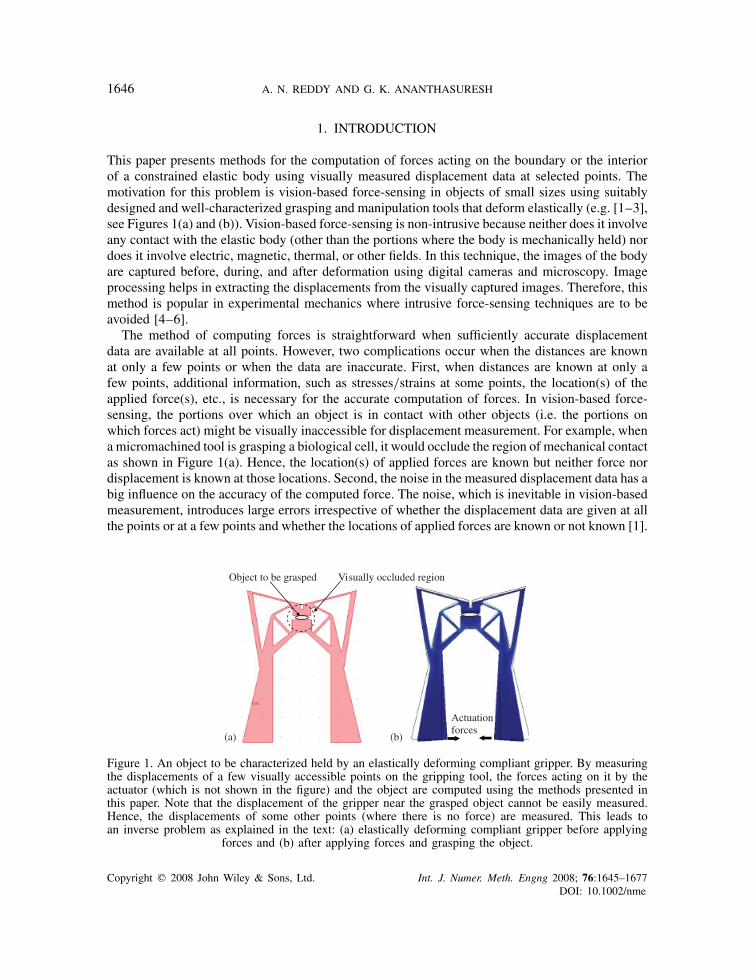
This paper presents methods for the computation of forces acting on the boundary or the interiorof a constrained elastic body using visually measured displacement data at selected points. Themotivation for this problem is vision-based force-sensing in objects of small sizes using suitablydesigned and well-characterized grasping and manipulation tools that deform elastically (e.g. [1–3],see Figures 1(a) and (b)). Vision-based force-sensing is non-intrusive because neither does it involveany contact with the elastic body (other than the portions where the body is mechanically held) nordoes it involve electric, magnetic, thermal, or other fields. In this technique, the images of the bodyare captured before, during, and after deformation using digital cameras and microscopy. Imageprocessing helps in extracting the displacements from the visually captured images. Therefore, thismethod is popular in experimental mechanics where intrusive force-sensing techniques are to beavoided [4–6].

The method of computing forces is straightforward when sufficiently accurate displacementdata are available at all points. However, two complications occur when the distances are knownat only a few points or when the data are inaccurate. First, when distances are known at only afew points, additional information, such as stresses/strains at some points, the location(s) of theapplied force(s), etc., is necessary for the accurate computation of forces. In vision-based force-sensing, the portions over which an object is in contact with other objects (i.e. the portions onwhich forces act) might be visually inaccessible for displacement measurement. For example, whena micromachined tool is grasping a biological cell, it would occlude the region of mechanical contactas shown in Figure 1(a). Hence, the location(s) of applied forces are known but neither force nordisplacement is known at those locations. Second, the noise in the measured displacement data has abig influence on the accuracy of the computed force. The noise, which is inevitable in vision-basedmeasurement, introduces large errors irrespective of whether the displacement data are given at allthe points or at a few points and whether the locations of applied forces are known or not known [1].

Object to be grasped Visually occluded region

(b)(a)

Actuationforces

Figure 1. An object to be characterized held by an elastically deforming compliant gripper. By measuringthe displacements of a few visually accessible points on the gripping tool, the forces acting on it by theactuator (which is not shown in the figure) and the object are computed using the methods presented inthis paper. Note that the displacement of the gripper near the grasped object cannot be easily measured.Hence, the displacements of some other points (where there is no force) are measured. This leads toan inverse problem as explained in the text: (a) elastically deforming compliant gripper before applying

forces and (b) after applying forces and grasping the object.

Copyright q 2008 John Wiley & Sons, Ltd. Int. J. Numer. Meth. Engng 2008; 76:1645–1677DOI: 10.1002/nme

ON COMPUTING THE FORCES FROM THE NOISY DISPLACEMENT DATA 1647

These two features make the problem considered in this paper a reconstruction-type inverse problem[7]. This is in contrast with the parameter extraction-type inverse problem or identification ofembedded entities (e.g. cracks, cavities, and inclusions) wherein the inhomogeneous materialproperties are estimated based on the measured displacements and forces [8].

In the reconstruction-type inverse problem in elasticity, the locations of applied forces andmaterial properties of the elastic body are assumed to be known. Here, we estimate forces anddisplacements at inaccessible locations from measured displacements at a few locations. This isknown as the Cauchy problem in elasticity [8, 7]. In particular, the focus of this paper is an inverseproblem to the geometrically non-linear elastic boundary value problem.

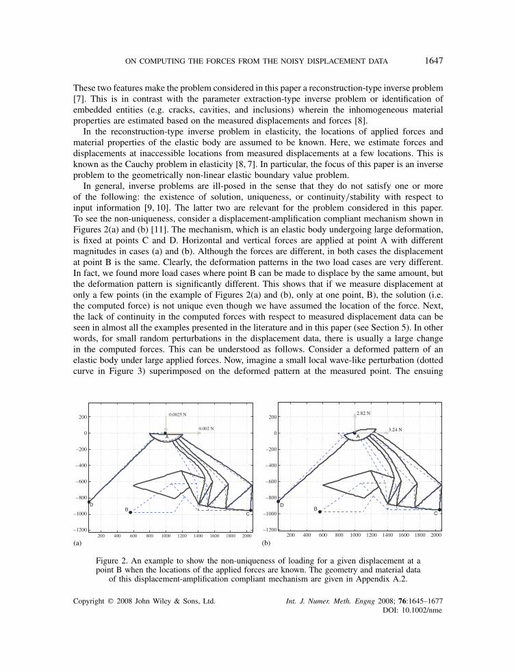
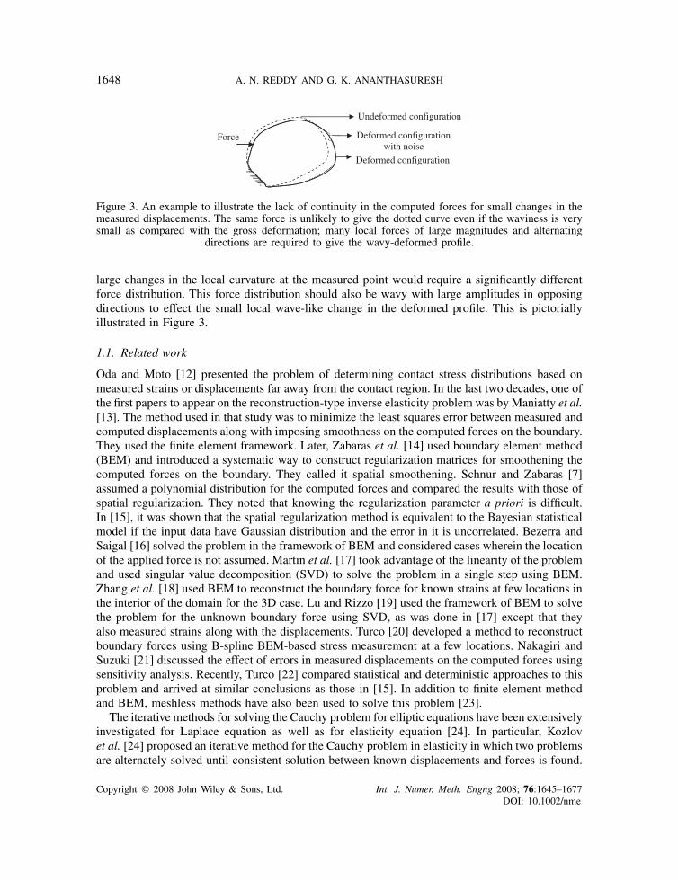
In general, inverse problems are ill-posed in the sense that they do not satisfy one or moreof the following: the existence of solution, uniqueness, or continuity/stability with respect toinput information [9, 10]. The latter two are relevant for the problem considered in this paper.To see the non-uniqueness, consider a displacement-amplification compliant mechanism shown inFigures 2(a) and (b) [11]. The mechanism, which is an elastic body undergoing large deformation,is fixed at points C and D. Horizontal and vertical forces are applied at point A with differentmagnitudes in cases (a) and (b). Although the forces are different, in both cases the displacementat point B is the same. Clearly, the deformation patterns in the two load cases are very different.In fact, we found more load cases where point B can be made to displace by the same amount, butthe deformation pattern is significantly different. This shows that if we measure displacement atonly a few points (in the example of Figures 2(a) and (b), only at one point, B), the solution (i.e.the computed force) is not unique even though we have assumed the location of the force. Next,the lack of continuity in the computed forces with respect to measured displacement data can beseen in almost all the examples presented in the literature and in this paper (see Section 5). In otherwords, for small random perturbations in the displacement data, there is usually a large changein the computed forces. This can be understood as follows. Consider a deformed pattern of anelastic body under large applied forces. Now, imagine a small local wave-like perturbation (dottedcurve in Figure 3) superimposed on the deformed pattern at the measured point. The ensuing

200 400 600 800 1000 1200 1400 1600 1800 2000 –1200

–1000

– 800

– 600

–400

–200

0

200

–1200

–1000

– 800

– 600

–400

–200

0

200

C

DB

A

0.0025 N

0.002 N

200 400 600 800 1000 1200 1400 1600 1800 2000

B

A

C

D

2.82 N

3.24 N

(a) (b)

Figure 2. An example to show the non-uniqueness of loading for a given displacement at apoint B when the locations of the applied forces are known. The geometry and material data

of this displacement-amplification compliant mechanism are given in Appendix A.2.



Force

Deformed configuration

Deformed configurationwith noise

Undeformed configuration

Figure 3. An example to illustrate the lack of continuity in the computed forces for small changes in themeasured displacements. The same force is unlikely to give the dotted curve even if the waviness is verysmall as compared with the gross deformation; many local forces of large magnitudes and alternating

directions are required to give the wavy-deformed profile.

large changes in the local curvature at the measured point would require a significantly differentforce distribution. This force distribution should also be wavy with large amplitudes in opposingdirections to effect the small local wave-like change in the deformed profile. This is pictoriallyillustrated in Figure 3.

1.1. Related work

Oda and Moto [12] presented the problem of determining contact stress distributions based onmeasured strains or displacements far away from the contact region. In the last two decades, one ofthe first papers to appear on the reconstruction-type inverse elasticity problem was byManiatty et al.[13]. The method used in that study was to minimize the least squares error between measured andcomputed displacements along with imposing smoothness on the computed forces on the boundary.They used the finite element framework. Later, Zabaras et al. [14] used boundary element method(BEM) and introduced a systematic way to construct regularization matrices for smoothening thecomputed forces on the boundary. They called it spatial smoothening. Schnur and Zabaras [7]assumed a polynomial distribution for the computed forces and compared the results with those ofspatial regularization. They noted that knowing the regularization parameter a priori is difficult.In [15], it was shown that the spatial regularization method is equivalent to the Bayesian statisticalmodel if the input data have Gaussian distribution and the error in it is uncorrelated. Bezerra andSaigal [16] solved the problem in the framework of BEM and considered cases wherein the locationof the applied force is not assumed. Martin et al. [17] took advantage of the linearity of the problemand used singular value decomposition (SVD) to solve the problem in a single step using BEM.Zhang et al. [18] used BEM to reconstruct the boundary force for known strains at few locations inthe interior of the domain for the 3D case. Lu and Rizzo [19] used the framework of BEM to solvethe problem for the unknown boundary force using SVD, as was done in [17] except that theyalso measured strains along with the displacements. Turco [20] developed a method to reconstructboundary forces using B-spline BEM-based stress measurement at a few locations. Nakagiri andSuzuki [21] discussed the effect of errors in measured displacements on the computed forces usingsensitivity analysis. Recently, Turco [22] compared statistical and deterministic approaches to thisproblem and arrived at similar conclusions as those in [15]. In addition to finite element methodand BEM, meshless methods have also been used to solve this problem [23].

The iterative methods for solving the Cauchy problem for elliptic equations have been extensivelyinvestigated for Laplace equation as well as for elasticity equation [24]. In particular, Kozlovet al. [24] proposed an iterative method for the Cauchy problem in elasticity in which two problemsare alternately solved until consistent solution between known displacements and forces is found.



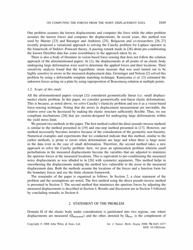
One problem assumes the known displacements and computes the force while the other problemassumes the known forces and computes the displacements. In recent years, this method wasused by Marine [23] and Baranger and Andrieux [25]. Belgacem and co-researchers [26, 27]recently proposed a variational approach to solving the Cauchy problem for Laplace operator inthe framework of Steklov–Poincare theory. A passing remark made in [26] about pre-conditioningthe known Dirichlet data has some resemblance to the approach taken by us.

There is also a body of literature in vision-based force-sensing that does not follow the solutionapproach of the aforementioned papers. In [1], the displacements at all points of an elastic bodyundergoing large deformation were used to determine the applied forces and their locations. Theirsensitivity analysis found that the logarithmic strain measure that was used turned out to behighly sensitive to errors in the measured displacement data. Greminger and Nelson [2] solved thisproblem by using a deformable template matching technique. Kamiyama et al. [3] estimated theunknown forces acting on a plate by using superposition of Boussinesq solution at multiple points.

1.2. Scope of this study

All the aforementioned papers (except [1]) considered geometrically linear (i.e. small displace-ments) elastic problem. In this paper, we consider geometrically non-linear elastic deformations.This is because, as noted above, we solve Cauchy’s elasticity problem and use it as a vision-basedforce-sensing technique. Noting that the errors in displacement measurement are inevitable, therelative error can be decreased by making the elastic structure sufficiently flexible. Thus, we usecompliant mechanisms [28] that are custom-designed for undergoing large deformations withinthe yield stress limit.

We present two methods in this paper. The first method (called the direct pseudo-inverse method)is similar to the method presented in [19] and one-step method presented in [17]. However, ourmethod necessarily becomes iterative because of the consideration of the geometric non-linearity.Numerical examples and experiments that we conducted indicate that this method, similar to theearlier methods, is prone to errors when deformations are large and when there is large noisein the data even in the case of small deformation. Therefore, the second method takes a newapproach to solve the Cauchy problem: here, we pose an optimization problem wherein smallperturbations in the measured displacements become the variables that are adjusted to minimizethe spurious forces at the measured locations. This is equivalent to pre-conditioning the measurednoisy displacements as was alluded to in [26] with symmetry arguments. This method helps insmoothening the displacements making the method less vulnerable to the noise in the measureddisplacement data. Both the methods assume the locations of the forces and a function form forthe boundary forces and use the finite element framework.

The remainder of the paper is organized as follows. In Section 2, a clear statement of theproblem and the assumptions are noted. The first method using the direct pseudo-inverse methodis presented in Section 3. The second method that minimizes the spurious forces by adjusting themeasured displacements is described in Section 4. Results and discussion are in Section 5 followedby concluding remarks in Section 6.

2. STATEMENT OF THE PROBLEM

Domain of the elastic body under consideration is partitioned into two regions, one wheredisplacements are measured (measured) and the other, denoted by free, is the complement of



tractionΓ

freeΓ

measuredΓ

freeΩ

fixedΓ

measuredΩ

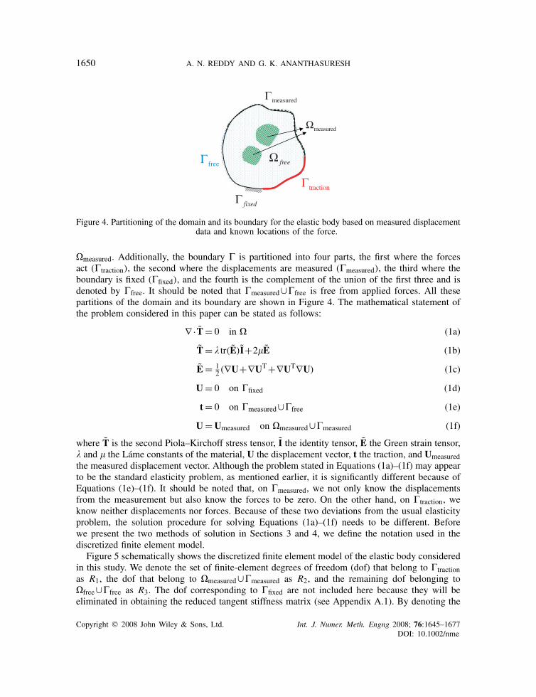
Figure 4. Partitioning of the domain and its boundary for the elastic body based on measured displacementdata and known locations of the force.

measured. Additionally, the boundary is partitioned into four parts, the first where the forcesact (traction), the second where the displacements are measured (measured), the third where theboundary is fixed (fixed), and the fourth is the complement of the union of the first three and isdenoted by free. It should be noted that measured∪free is free from applied forces. All thesepartitions of the domain and its boundary are shown in Figure 4. The mathematical statement ofthe problem considered in this paper can be stated as follows:

∇ ·T= 0 in (1a)

T= tr(E)I+2E (1b)

E= 12 (∇U+∇UT+∇UT∇U) (1c)

U= 0 on fixed (1d)

t= 0 on measured∪free (1e)

U=Umeasured on measured∪measured (1f)

where T is the second Piola–Kirchoff stress tensor, I the identity tensor, E the Green strain tensor, and the Lame constants of the material, U the displacement vector, t the traction, and Umeasuredthe measured displacement vector. Although the problem stated in Equations (1a)–(1f) may appearto be the standard elasticity problem, as mentioned earlier, it is significantly different because ofEquations (1e)–(1f). It should be noted that, on measured, we not only know the displacementsfrom the measurement but also know the forces to be zero. On the other hand, on traction, weknow neither displacements nor forces. Because of these two deviations from the usual elasticityproblem, the solution procedure for solving Equations (1a)–(1f) needs to be different. Beforewe present the two methods of solution in Sections 3 and 4, we define the notation used in thediscretized finite element model.

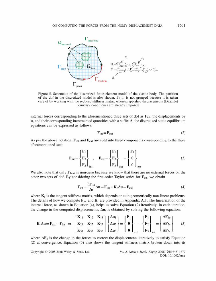
Figure 5 schematically shows the discretized finite element model of the elastic body consideredin this study. We denote the set of finite-element degrees of freedom (dof) that belong to tractionas R1, the dof that belong to measured∪measured as R2, and the remaining dof belonging tofree∪free as R3. The dof corresponding to fixed are not included here because they will beeliminated in obtaining the reduced tangent stiffness matrix (see Appendix A.1). By denoting the



tractionΓ

freeΓ

measuredΓ

freeΩ

fixedΓ

measuredΩ

measured free

traction measured free fixed

Ω = Ω ∪ Ω

Γ = Γ ∪ Γ ∪ Γ ∪ Γ

1R

2R3R

Figure 5. Schematic of the discretized finite element model of the elastic body. The partitionof the dof in the discretized model is also shown. fixed is not grouped because it is takencare of by working with the reduced stiffness matrix wherein specified displacements (Dirichlet

boundary conditions) are already imposed.

internal forces corresponding to the aforementioned three sets of dof as Fint, the displacements byu, and their corresponding incremented quantities with a suffix , the discretized static equilibriumequations can be expressed as follows:

Fint=Fext (2)

As per the above notation, Fint and Fext are split into three components corresponding to the threeaforementioned sets:

Fint=

⎧⎪⎨⎪⎩F1

F2

F3

⎫⎪⎬⎪⎭

int

, Fext=

⎧⎪⎨⎪⎩F1

F2

F3

⎫⎪⎬⎪⎭

ext

=

⎧⎪⎨⎪⎩F1

0

0

⎫⎪⎬⎪⎭

ext

(3)

We also note that only F1ext is non-zero because we know that there are no external forces on theother two sets of dof. By considering the first-order Taylor series for Fint, we obtain

Fint+ Fint

uu=Fint+Ktu=Fext (4)

where Kt is the tangent stiffness matrix, which depends on u in geometrically non-linear problems.The details of how we compute Fint and Kt are provided in Appendix A.1. The linearization of theinternal force, as shown in Equation (4), helps us solve Equation (2) iteratively. In each iteration,the change in the computed displacements, u, is obtained by solving the following equation:

Ktu=Fext−Fint ⇒⎡⎢⎣K11 K12 K13

K21 K22 K23

K31 K32 K33

⎤⎥⎦

⎧⎪⎨⎪⎩

u1

u2

u3

⎫⎪⎬⎪⎭=

⎧⎪⎨⎪⎩F1

0

0

⎫⎪⎬⎪⎭

ext

−

⎧⎪⎨⎪⎩F1

F2

F3

⎫⎪⎬⎪⎭

int

=

⎧⎪⎨⎪⎩

F1c

F2c

F3c

⎫⎪⎬⎪⎭ (5)

where Fc is the change in the forces to correct the displacements iteratively to satisfy Equation(2) at convergence. Equation (5) also shows the tangent stiffness matrix broken down into its



constituents corresponding to the three sets. Now, the problem reduces to determining F1ext.Equation (5) will be used in the two methods of solution to this problem as presented in thefollowing two sections.

3. DIRECT PSEUDO-INVERSE METHOD (DPIM)

The main idea of this method is to keep the measured displacement vector, u2, unchanged eventhough we know that there might be measurement errors in it. Therefore, in the iterative procedure tosolve the problem in Equation (2), when we use the linearized iterative equation (i.e. Equation (5)),u2 will be a null vector:⎡

⎢⎣K11 K12 K13

K21 K22 K23

K31 K32 K33

⎤⎥⎦

⎧⎪⎨⎪⎩

u1

0

u3

⎫⎪⎬⎪⎭=

⎧⎪⎨⎪⎩F1

0

0

⎫⎪⎬⎪⎭

ext

−

⎧⎪⎨⎪⎩F1

F2

F3

⎫⎪⎬⎪⎭

int

=

⎧⎪⎨⎪⎩

F1c

F2c

F3c

⎫⎪⎬⎪⎭ (6)

We initiate the method by assuming that u1 and u3 are null vectors and u2 is the measureddisplacement vector. Using these, we compute Fint. Now, by using the last row of Equation (6),we obtain

u3=K−133 (F3c−K31u1)=K−1

33 (−F3int−K31u1) (7)

By substituting u3 from Equation (7) into the second row of Equation (6), we obtain

[K21−K23K−133 K31]u1 = DF2c−K23K

−133 F3c

= −F2int+K23K−133 F3int (8)

Because [K21−K23K−133 K31] is not a square matrix in general, we need to use pseudo-inverse to

solve Equation (8). After this, we substitute u1 and u3 from Equations (8) and (7), respectively,into the first row of Equation (6) to compute F1c. This correction is used to compute the unknownexternal force on the traction boundary:

F1ext=F1c+F1int (9)

Now, we also update the displacements, u1 and u3:

unew1 = u1+uold1

unew3 = u3+uold3(10)

Note that u2 does not need to be updated because in this method we assume that u2 is a nullvector as noted above. This procedure is repeated until the norms of u1 and u3 are negligiblysmall.

When the above algorithm converges, F3int is driven to a null vector because the third row ofEquation (6) is exactly satisfied. However, F2int in general does not approach a null vector becauseof the pseudo-inverse solution of the second row of Equation (6). This issue is addressed in oursecond method. This issue aside, it should be noted that there is no guarantee that this iterativealgorithm always converges. Hence, we modify this below by assuming a function form for F1ext.



Assuming a suitable function form of an unknown quantity in inverse problems leads to regu-larization. For example, Schnur and Zabaras [7] and Bezerra and Saigal [16] assumed the functionform for the unknown force and obtained regularized solution. The way in which we use thefunction form for the unknown forces is different from these two and other papers because thesolution procedure presented above is different.

For a chosen function form on traction, in the discretized finite element model, we can expressthe following:

F1ext=[P]a (11)

where P is a coefficient matrix that fits the function form onto the discretized model and a is thevector of unknown coefficients in the assumed function form. Now, since F1ext=F1int, we definea least squares error, , for F1int:

=(Pa−F1int)T(Pa−F1int) (12)

Minimization of this error with respect to a yields

a=0 ⇒ a=[PTP]−1PTF1int (13)

By substituting the value of a from Equation (13) into Equations (11) and (9), we obtain anestimate for F1c as follows:

F1c=Pa−F1int=[P(PTP)−1PT−I]F1int (14)

This is an additional piece of information in solving Equation (6). Previously, only the second rowwas used to compute u1 as shown in Equation (8). Now, we use the additional information inEquation (14) (which came from the assumed function form of F1ext) by using the first and secondrows of Equation (6) simultaneously to compute u1:[

K11−K13K−133 K31

K21−K23K−133 K31

]u1=

[P(PTP)−1PT−I]F1int+K13K−133 F3int

−F2int+K23K−133 F3int

(15)

This modification is an improvement over the earlier procedure because it ensures that the computedtraction follows the known function form. However, there is an inherent problem in this method,which is also applicable to other methods. The problem is that unwanted forces arise at thedisplacement measurement points. This is because even the modified algorithm (i.e. Equation (15))does not make F2int a null vector, especially when the errors in the measured displacements arelarge. The non-zero value of F2ext, which is equal to F2int when F2c becomes zero at convergence,leads to spurious forces on the measured dof (i.e. R2 in Figure 5). These forces are called spuriousbecause we assumed that there are no external forces at the measured dof. The first numericalexample in Section 5 illustrates the effect of noise on the appearance of spurious forces. In thefollowing section, we present a method that minimizes such spurious forces.

4. METHOD OF MINIMIZING SPURIOUS FORCES (MMSF)

In Section 1, we note that a small perturbation in the measured displacement data necessitatesa large change in the computed force to accommodate that perturbation. This is also pictorially



illustrated in Figure 3. Earlier work focused on regularizing the computed force. Here, we wantto regularize/pre-condition the measured displacement itself because we know that measureddisplacement data using computer vision would inevitably be noisy. We do this by allowing smallperturbations in the measured displacement data, u2. We use these perturbations as variables in anoptimization problem that minimizes the norm of the spurious forces that arise at the measureddof, F2. Thus, this method is called the method of minimizing spurious forces (MMSF). It helpspre-condition the measured displacement data while helping also to regularize the computed forcedata. The minimization problem is mathematically stated as follows:

Minimizeu2a

FT2F2

Subject to umin2a u2aumax

2a

(P1)

where

umin2a =(1−/100)u2

umax2a =(1+/100)u2

(16)

with denoting the maximum percent error in the measured data.The method of computing F2 in problem (P1) is the same as the DPIM presented in Section 3

with the difference that u2=u2a. This means that in each iteration of the optimization procedure,we need to solve DPIM once. In order to make the optimization solution procedure computationallyefficient, we compute the gradients of the objective function analytically (instead of using finitedifference methods) as shown below.

4.1. Analytical computation of the gradients

The gradient of the objective function in problem (P1) is given by

(FT2F2)

u2=2

(FT2 )

u2F2 (17)

By using the second and third rows of Equation (5), we obtain

F2c=[K22−K23K−133 K32]u2+[K21−K23K

−133 K31]u1+K23K

−133 F3c (18)

From Equations (18) and (17), the gradient can now be obtained as

(FT2F2)

u2=2[K22−K23K

−133 K32]F2 (19)

The fmincon routine in the MATLAB optimization toolbox was used to solve the optimizationproblem. Sequential quadratic programming combined with the trust region method is used byfmincon. Results of DPIM and MMSF are presented in the following section.

5. RESULTS AND DISCUSSION

In this section, seven numerical examples and one experimental example are presented. In thenumerical examples, the displacement data are generated numerically by using the computed



displacements with known applied forces. Thus, in these examples we know the correct values ofthe forces. Then, ‘noise’ is added to it using rand function in Matlab. The noise level is variedby using % to study the effects of increased noise. The rand function gives a value within therange [0,1]. Therefore, u2 with noise can be expressed as follows:

unoisy2i=

(1+ (−1+2(rand))

100

)u2i (20)

where the subscript i refers to the i th dof. Thus, the rand function is invoked separately for eachdof in u2. This gives non-uniform noise over the measured portion of the elastic body, which ismore realistic than giving the same noise everywhere. The noisy data generated in this manner areused to estimate the forces. This helps in validating the accuracy of the two methods presented inthis paper. We used 4-noded and 9-noded quadrilateral elements as well as co-rotational 2D beamelements. The elastic bodies considered are an arch beam, a rectangular sheet, a displacement-amplification compliant mechanism, and a slender rectangular sheet that acts like a cantilever. Allthe numerical examples were solved using both DPIM and MMSF. The experimental example wassolved using only MMSF, which is superior to DPIM.

5.1. Example 1: an effect of the noise and motivation for MMSF

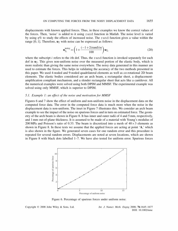
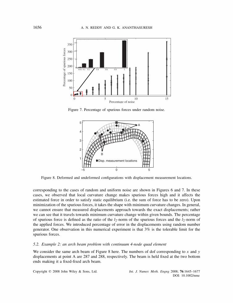
Figures 6 and 7 show the effect of uniform and non-uniform noise in the displacement data on thecomputed force data. The error in the computed force data is much more when the noise in thedisplacement data is non-uniform. The inset in Figure 7 illustrates this. We consider an arch beamexample to see the impact of the noise on spurious forces and in turn on estimated force. The geom-etry of the arch beam is shown in Figure 8. It has inner and outer radii of 4 and 5mm, respectively,and 1mm out-of-plane thickness. It is assumed to be made of a material with Young’s modulus of200MPa and Poisson’s ratio of 0.33. The beam is discretized into a mesh of 40×3 elements asshown in Figure 8. In these tests we assume that the applied forces are acting at point ‘A,’ whichis also shown in the figure. We generated seven cases for one random error and this procedure isrepeated for several random errors. Displacements are noted at seven locations, which are shownin Figure 8 with black dots labelled 1–7. We have also tested for uniform error. Spurious forces

0 5 10 15

2

4

6

8

10

Percentage of uniform noise

Perc

enta

ge o

f sp

urio

us f

orce

Figure 6. Percentage of spurious forces under uniform noise.



0 5 10 150

50

100

150

200

250

300

350

Percentage of noise

Perc

enta

ge o

f sp

urio

us f

orce

s

0.01 0.1 0.2 0.4 0.6 0.8 10

5

10

15

Figure 7. Percentage of spurious forces under random noise.

–5 0 5

1

2

3

4

5

Disp. measurement locations

13

2

5

64

7

B

A

Figure 8. Deformed and undeformed configurations with displacement measurement locations.

corresponding to the cases of random and uniform noise are shown in Figures 6 and 7. In thesecases, we observed that local curvature change makes spurious forces high and it affects theestimated force in order to satisfy static equilibrium (i.e. the sum of force has to be zero). Uponminimization of the spurious forces, it takes the shape with minimum curvature changes. In general,we cannot ensure that measured displacements approach towards the exact displacements; ratherwe can see that it travels towards minimum curvature change within given bounds. The percentageof spurious force is defined as the ratio of the l2-norm of the spurious forces and the l2-norm ofthe applied forces. We introduced percentage of error in the displacements using random numbergenerator. One observation in this numerical experiment is that 3% is the tolerable limit for thespurious forces.

5.2. Example 2: an arch beam problem with continuum 4-node quad element

We consider the same arch beam of Figure 8 here. The numbers of dof corresponding to x and ydisplacements at point A are 287 and 288, respectively. The beam is held fixed at the two bottomends making it a fixed-fixed arch beam.



287 288

–5

–4

– 3

–2

–1

0

1

2

3

4

Degree of freedom

Forc

e [N

]

Computed forceApplied force

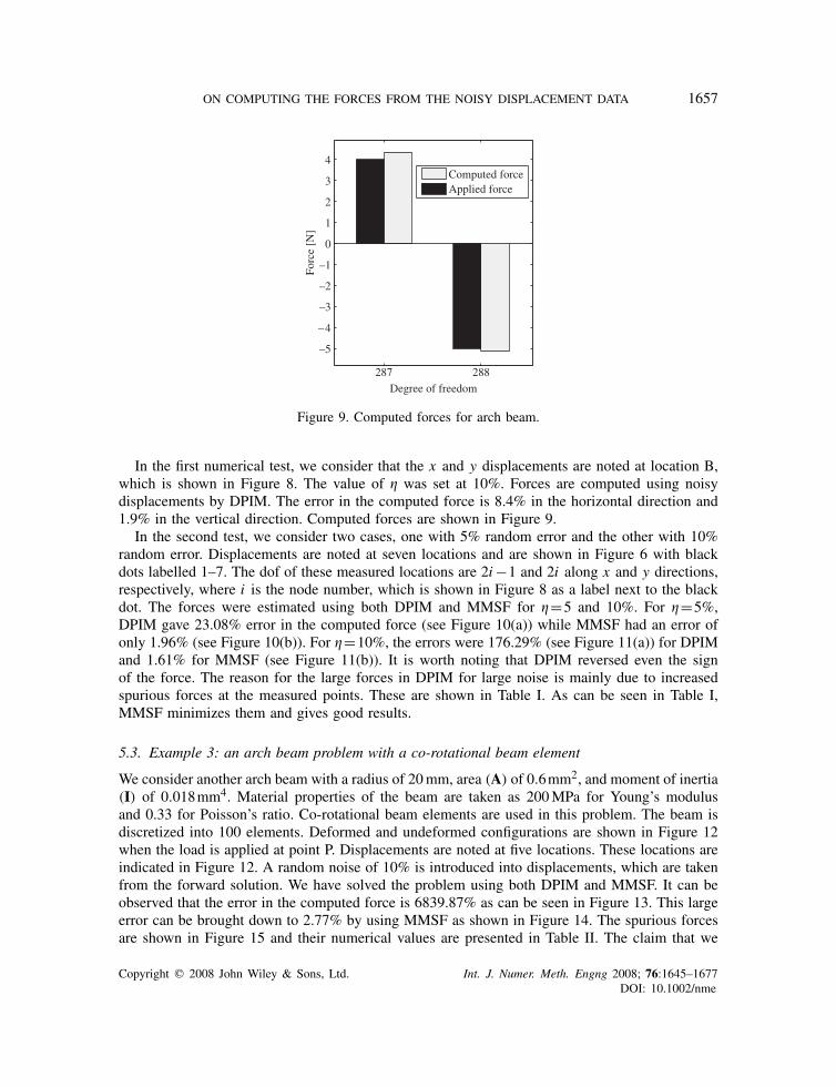
Figure 9. Computed forces for arch beam.

In the first numerical test, we consider that the x and y displacements are noted at location B,which is shown in Figure 8. The value of was set at 10%. Forces are computed using noisydisplacements by DPIM. The error in the computed force is 8.4% in the horizontal direction and1.9% in the vertical direction. Computed forces are shown in Figure 9.

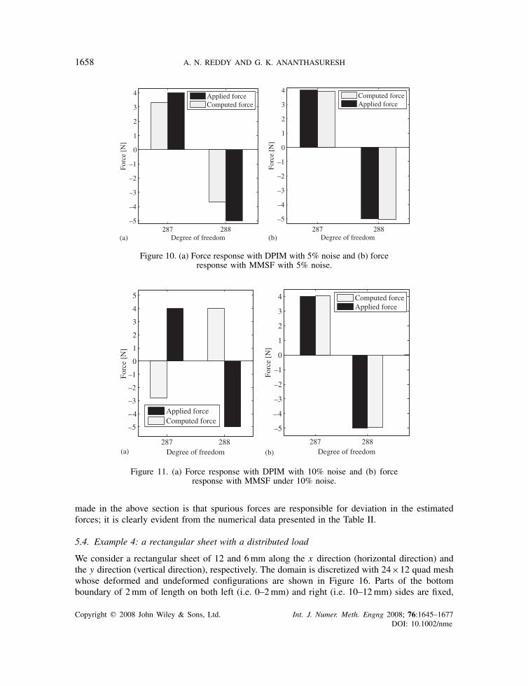
In the second test, we consider two cases, one with 5% random error and the other with 10%random error. Displacements are noted at seven locations and are shown in Figure 6 with blackdots labelled 1–7. The dof of these measured locations are 2i−1 and 2i along x and y directions,respectively, where i is the node number, which is shown in Figure 8 as a label next to the blackdot. The forces were estimated using both DPIM and MMSF for =5 and 10%. For =5%,DPIM gave 23.08% error in the computed force (see Figure 10(a)) while MMSF had an error ofonly 1.96% (see Figure 10(b)). For =10%, the errors were 176.29% (see Figure 11(a)) for DPIMand 1.61% for MMSF (see Figure 11(b)). It is worth noting that DPIM reversed even the signof the force. The reason for the large forces in DPIM for large noise is mainly due to increasedspurious forces at the measured points. These are shown in Table I. As can be seen in Table I,MMSF minimizes them and gives good results.

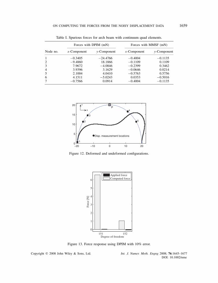
5.3. Example 3: an arch beam problem with a co-rotational beam element

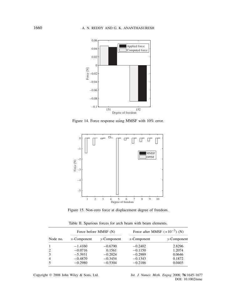
We consider another arch beam with a radius of 20mm, area (A) of 0.6mm2, and moment of inertia(I) of 0.018mm4. Material properties of the beam are taken as 200MPa for Young’s modulusand 0.33 for Poisson’s ratio. Co-rotational beam elements are used in this problem. The beam isdiscretized into 100 elements. Deformed and undeformed configurations are shown in Figure 12when the load is applied at point P. Displacements are noted at five locations. These locations areindicated in Figure 12. A random noise of 10% is introduced into displacements, which are takenfrom the forward solution. We have solved the problem using both DPIM and MMSF. It can beobserved that the error in the computed force is 6839.87% as can be seen in Figure 13. This largeerror can be brought down to 2.77% by using MMSF as shown in Figure 14. The spurious forcesare shown in Figure 15 and their numerical values are presented in Table II. The claim that we



287 288 –5

–4

–3

–2

–1

0

1

2

3

4

Degree of freedom

Forc

e[N

]

Applied forceComputed force

287 288

– 5

–4

–3

–2

–1

0

1

2

3

4

Degree of freedom

Forc

e [N

]


(a) (b)

Figure 10. (a) Force response with DPIM with 5% noise and (b) forceresponse with MMSF with 5% noise.

287 288

–5

–4

– 3

–2

–1

0

1

2

3

4

5

Degree of freedom

Forc

e [N

]


287 288

–5

– 4

–3

–2

– 1

0

1

2

3

4

Degree of freedom

Forc

e [N

]


(a) (b)

Figure 11. (a) Force response with DPIM with 10% noise and (b) forceresponse with MMSF under 10% noise.

made in the above section is that spurious forces are responsible for deviation in the estimatedforces; it is clearly evident from the numerical data presented in the Table II.

5.4. Example 4: a rectangular sheet with a distributed load

We consider a rectangular sheet of 12 and 6mm along the x direction (horizontal direction) andthe y direction (vertical direction), respectively. The domain is discretized with 24×12 quad meshwhose deformed and undeformed configurations are shown in Figure 16. Parts of the bottomboundary of 2mm of length on both left (i.e. 0–2mm) and right (i.e. 10–12mm) sides are fixed,



Table I. Spurious forces for arch beam with continuum quad elements.

Forces with DPIM (mN) Forces with MMSF (mN)

Node no. x-Component y-Component x-Component y-Component

1 −0.3405 −24.4766 −0.4004 −0.11352 −9.4860 18.1866 −0.1109 0.11093 7.9672 −4.0846 −0.2399 0.34624 3.9396 3.1629 −0.0646 0.02145 2.1004 4.0410 −0.5763 0.57566 4.1511 −5.0243 0.0353 −0.50167 −0.7566 0.0914 −0.4004 −0.1135

–20 –10 0 10 200

5

10

15

20

Disp. measurement locations

P

1

2

3

4

5

X

Y

Figure 12. Deformed and undeformed configurations.

151 152

0

1

2

3

4

5

6

Degree of freedom

Forc

e [N

]


Figure 13. Force response using DPIM with 10% error.



151 152 –0.1

–0.08

–0.06

– 0.04

– 0.02

0

0.02

0.04

0.06

Degree of freedom

Forc

e [N

]


Figure 14. Force response using MMSF with 10% error.

1 2 3 4 5 6 7 8 9 10

– 5

–4

– 3

– 2

–1

0

Degree of freedom

Forc

e [N

]

MMSFDPIM

Figure 15. Non-zero force at displacement degree of freedom.

Table II. Spurious forces for arch beam with beam elements.

Force before MMSF (N) Force after MMSF (×10−3) (N)


1 −1.4160 −0.6790 −0.2402 2.82962 −0.0716 0.1561 −0.1150 1.20743 −5.3931 −0.2024 −0.2989 0.06464 −0.4870 −0.3454 −0.1343 0.18725 −0.2980 −0.5304 −0.2186 0.0403



0 2 4 6 8 10 120

1

2

3

4

5

6

7

8

Disp. measurement nodes

1

2

3

45

7 68

9

309310

311312

313

314315

316317

Nodes under tractionX

Y

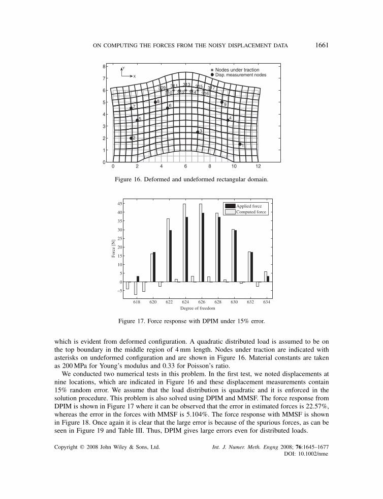
Figure 16. Deformed and undeformed rectangular domain.

618 620 622 624 626 628 630 632 634

0

5

–5

10

15

20

25

30

35

40

45

Degree of freedom

Forc

e [N

]


Figure 17. Force response with DPIM under 15% error.

which is evident from deformed configuration. A quadratic distributed load is assumed to be onthe top boundary in the middle region of 4mm length. Nodes under traction are indicated withasterisks on undeformed configuration and are shown in Figure 16. Material constants are takenas 200MPa for Young’s modulus and 0.33 for Poisson’s ratio.

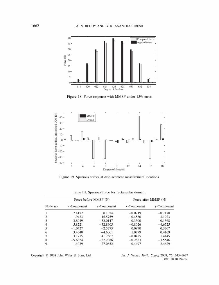
We conducted two numerical tests in this problem. In the first test, we noted displacements atnine locations, which are indicated in Figure 16 and these displacement measurements contain15% random error. We assume that the load distribution is quadratic and it is enforced in thesolution procedure. This problem is also solved using DPIM and MMSF. The force response fromDPIM is shown in Figure 17 where it can be observed that the error in estimated forces is 22.57%,whereas the error in the forces with MMSF is 5.104%. The force response with MMSF is shownin Figure 18. Once again it is clear that the large error is because of the spurious forces, as can beseen in Figure 19 and Table III. Thus, DPIM gives large errors even for distributed loads.



618 620 622 624 626 628 630 632 634

0

5

10

15

20

25

30

35

40

Degree of freedom

Forc

e [N

]


Figure 18. Force response with MMSF under 15% error.

2 4 6 8 10 12 14 16 18 –40

–30

–20

–10

0

10

20

30

40

Degree of freedom

Spur

ious

for

ce a

t dis

p. p

resc

ribe

d D

OF

[N]

MMSFDPIM

Figure 19. Spurious forces at displacement measurement locations.

Table III. Spurious force for rectangular domain.

Force before MMSF (N) Force after MMSF (N)


1 7.4152 8.1054 −0.0719 −0.71702 −1.9423 15.5759 −0.4560 3.19233 3.8049 −33.0147 0.3500 −0.13684 5.8221 −32.8605 −0.8026 −4.67255 −1.0427 −2.5773 0.0870 0.37076 3.4340 −4.6061 1.0799 0.41697 3.1715 41.7567 −0.0485 1.41458 −5.6324 −32.2386 −0.2833 −3.55469 1.4039 27.0852 0.4497 2.4629



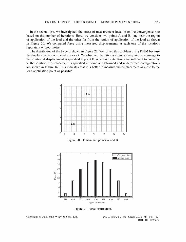
In the second test, we investigated the effect of measurement location on the convergence ratebased on the number of iterations. Here, we consider two points A and B, one near the regionof application of the load and the other far from the region of application of the load as shownin Figure 20. We computed force using measured displacements at each one of the locationsseparately without noise.

The distribution of the force is shown in Figure 21. We solved this problem using DPIM becausethe displacements considered are exact. We observed that 86 iterations are required to converge tothe solution if displacement is specified at point B, whereas 19 iterations are sufficient to convergeto the solution if displacement is specified at point A. Deformed and undeformed configurationsare shown in Figure 16. This indicates that it is better to measure the displacement as close to theload application point as possible.

0 2 4 6 8 10 120

1

2

3

4

5

6

A

B

Figure 20. Domain and points A and B.

618 620 622 624 626 628 630 632 6340

5

10

15

20

25

30

35

40

45

Degree of freedom

Forc

e [N

]


Figure 21. Force distribution.



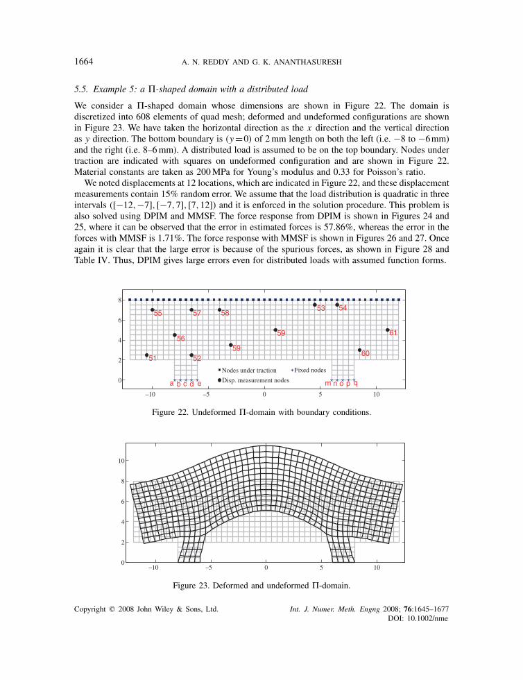
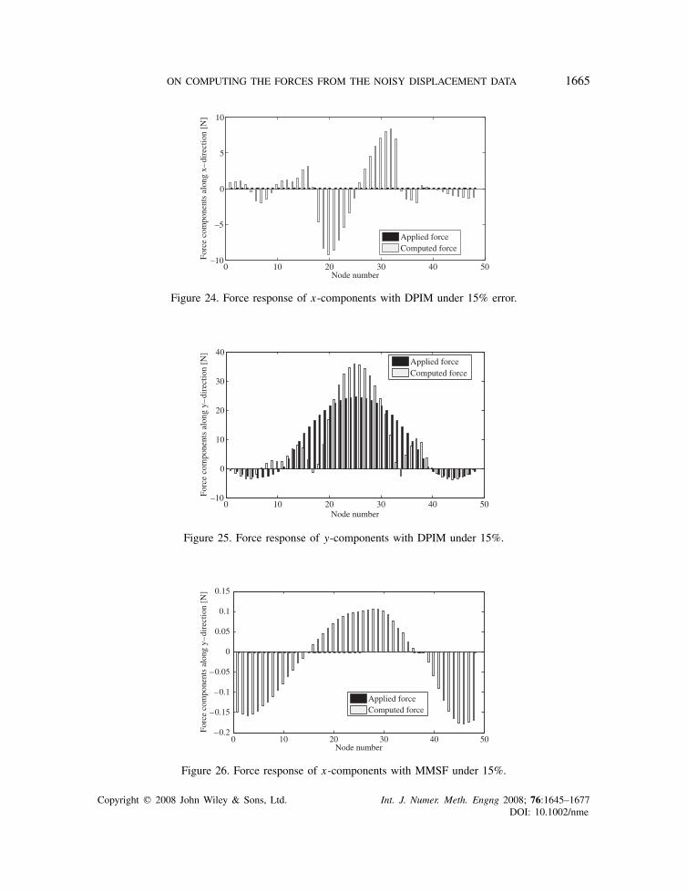
5.5. Example 5: a -shaped domain with a distributed load

We consider a -shaped domain whose dimensions are shown in Figure 22. The domain isdiscretized into 608 elements of quad mesh; deformed and undeformed configurations are shownin Figure 23. We have taken the horizontal direction as the x direction and the vertical directionas y direction. The bottom boundary is (y=0) of 2mm length on both the left (i.e. −8 to −6mm)and the right (i.e. 8–6mm). A distributed load is assumed to be on the top boundary. Nodes undertraction are indicated with squares on undeformed configuration and are shown in Figure 22.Material constants are taken as 200MPa for Young’s modulus and 0.33 for Poisson’s ratio.

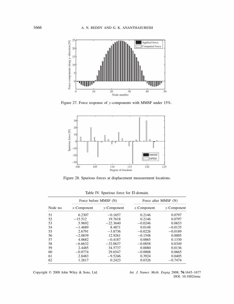
We noted displacements at 12 locations, which are indicated in Figure 22, and these displacementmeasurements contain 15% random error. We assume that the load distribution is quadratic in threeintervals ([−12,−7], [−7,7], [7,12]) and it is enforced in the solution procedure. This problem isalso solved using DPIM and MMSF. The force response from DPIM is shown in Figures 24 and25, where it can be observed that the error in estimated forces is 57.86%, whereas the error in theforces with MMSF is 1.71%. The force response with MMSF is shown in Figures 26 and 27. Onceagain it is clear that the large error is because of the spurious forces, as shown in Figure 28 andTable IV. Thus, DPIM gives large errors even for distributed loads with assumed function forms.

–10 –5 0 5 10

0

2

4

6

8

51 52

53 5455

56

57 58

59

59

60

61

a b c d e m n o p q

Nodes under traction

Disp. measurement nodes

Fixed nodes

Figure 22. Undeformed -domain with boundary conditions.

– 10 – 5 0 5 100

2

4

6

8

10

Figure 23. Deformed and undeformed -domain.



0 10 20 30 40 50 –10

– 5

0

5

10

Node number

Forc

e co

mpo

nent

s al

ong

x –di

rect

ion

[N]


Figure 24. Force response of x-components with DPIM under 15% error.

0 10 20 30 40 50 –10

0

10

20

30

40

Node number

Forc

e co

mpo

nent

s al

ong

y– di

rect

ion

[N]


Figure 25. Force response of y-components with DPIM under 15%.

0 10 20 30 40 50 –0.2

– 0.15

– 0.1

–0.05

0

0.05

0.1

0.15

Node number

Forc

e co

mpo

nent

s al

ong

y– di

rect

ion

[N]


Figure 26. Force response of x-components with MMSF under 15%.



0 10 20 30 40 50

0

5

10

15

20

25

Node number

Forc

e co

mpo

nent

s al

ong

y– di

rect

ion

[N]


Figure 27. Force response of y-components with MMSF under 15%.

100 105 110 115 120 125

–30

–20

– 10

0

10

20

30

Degree of freedom

Spur

ious

for

ce [

N]

MMSFDPIM

Figure 28. Spurious forces at displacement measurement locations.

Table IV. Spurious force for -domain.

Force before MMSF (N) Force after MMSF (N)


51 6.2307 −0.1657 0.2146 0.079752 −15.512 19.7618 0.2146 0.079753 5.9692 −22.3640 −0.0246 0.065354 −1.4689 8.4871 0.0148 −0.013555 2.6791 −3.8736 −0.0226 −0.018956 −2.0839 12.9261 −0.1548 0.000557 4.0682 −0.4187 0.0065 0.133058 −6.6632 −32.0637 −0.0858 0.034959 2.4485 34.5737 0.0080 0.013660 −0.0774 29.6547 −0.0008 0.066561 2.8483 −9.5246 0.3924 0.040562 1.2617 0.2423 0.0326 −0.7474



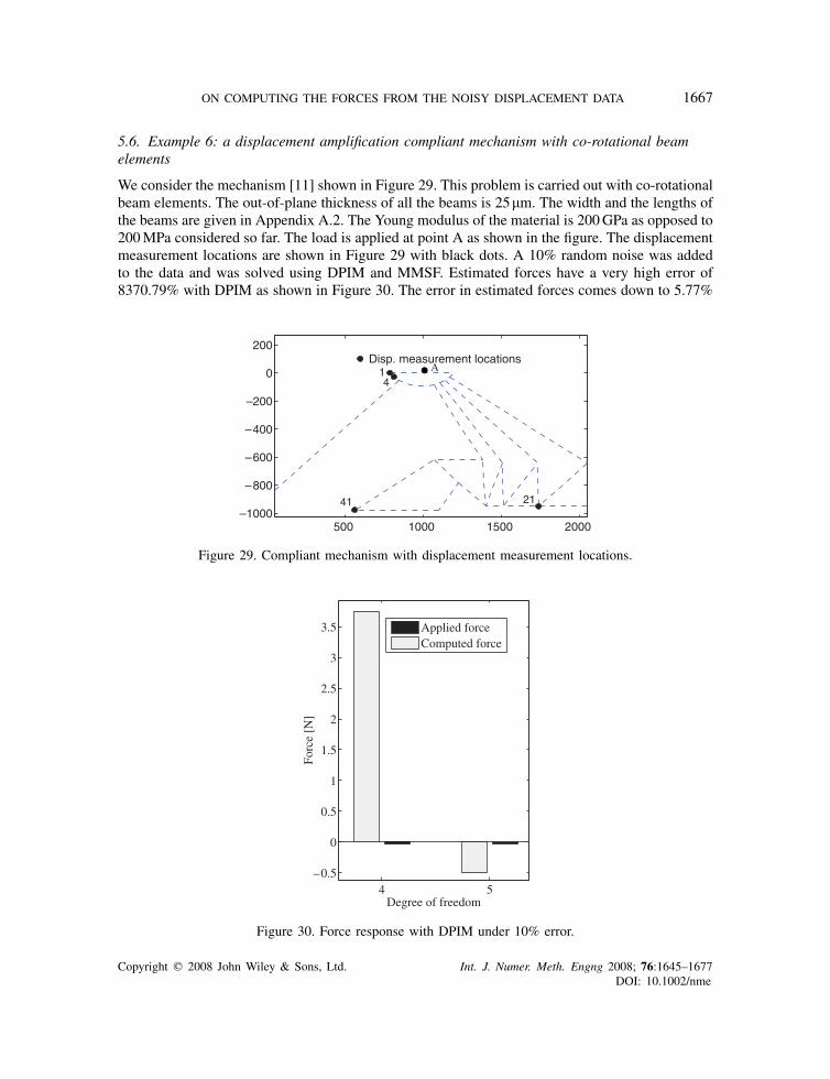
5.6. Example 6: a displacement amplification compliant mechanism with co-rotational beamelements

We consider the mechanism [11] shown in Figure 29. This problem is carried out with co-rotationalbeam elements. The out-of-plane thickness of all the beams is 25m. The width and the lengths ofthe beams are given in Appendix A.2. The Young modulus of the material is 200GPa as opposed to200MPa considered so far. The load is applied at point A as shown in the figure. The displacementmeasurement locations are shown in Figure 29 with black dots. A 10% random noise was addedto the data and was solved using DPIM and MMSF. Estimated forces have a very high error of8370.79% with DPIM as shown in Figure 30. The error in estimated forces comes down to 5.77%

500 1000 1500 2000 –1000

–800

– 600

– 400

– 200

0

200Disp. measurement locations

14

2141

A

Figure 29. Compliant mechanism with displacement measurement locations.

4 5 –0.5

0

0.5

1

1.5

2

2.5

3

3.5

Degree of freedom

Forc

e [N

]


Figure 30. Force response with DPIM under 10% error.



4 5

–0.035

–0.03

–0.025

–0.02

–0.015

– 0.01

–0.005

0

Degree of freedom

Forc

e [N

] Applied forceComputed force

Figure 31. Force response with MMSF under 10% error.

Figure 32. Cantilever beam with displacement measurement locations.

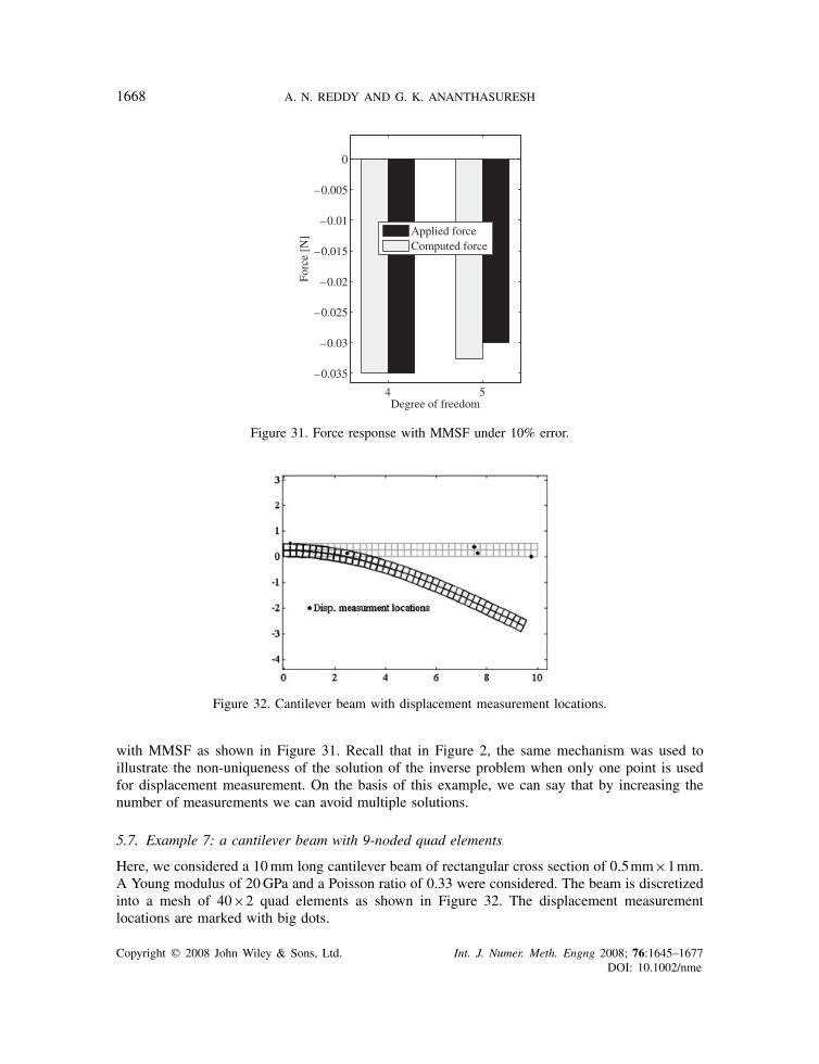
with MMSF as shown in Figure 31. Recall that in Figure 2, the same mechanism was used toillustrate the non-uniqueness of the solution of the inverse problem when only one point is usedfor displacement measurement. On the basis of this example, we can say that by increasing thenumber of measurements we can avoid multiple solutions.

5.7. Example 7: a cantilever beam with 9-noded quad elements

Here, we considered a 10mm long cantilever beam of rectangular cross section of 0.5mm×1mm.A Young modulus of 20GPa and a Poisson ratio of 0.33 were considered. The beam is discretizedinto a mesh of 40×2 quad elements as shown in Figure 32. The displacement measurementlocations are marked with big dots.



809 810

– 2

–1.8

–1.6

– 1.4

– 1.2

–1

– 0.8

–0.6

–0.4

–0.2

0

Degree of freedom

For

ce [

N]


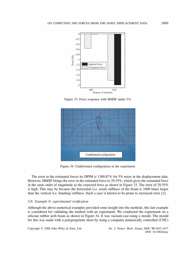
Figure 33. Force response with MMSF under 5%.

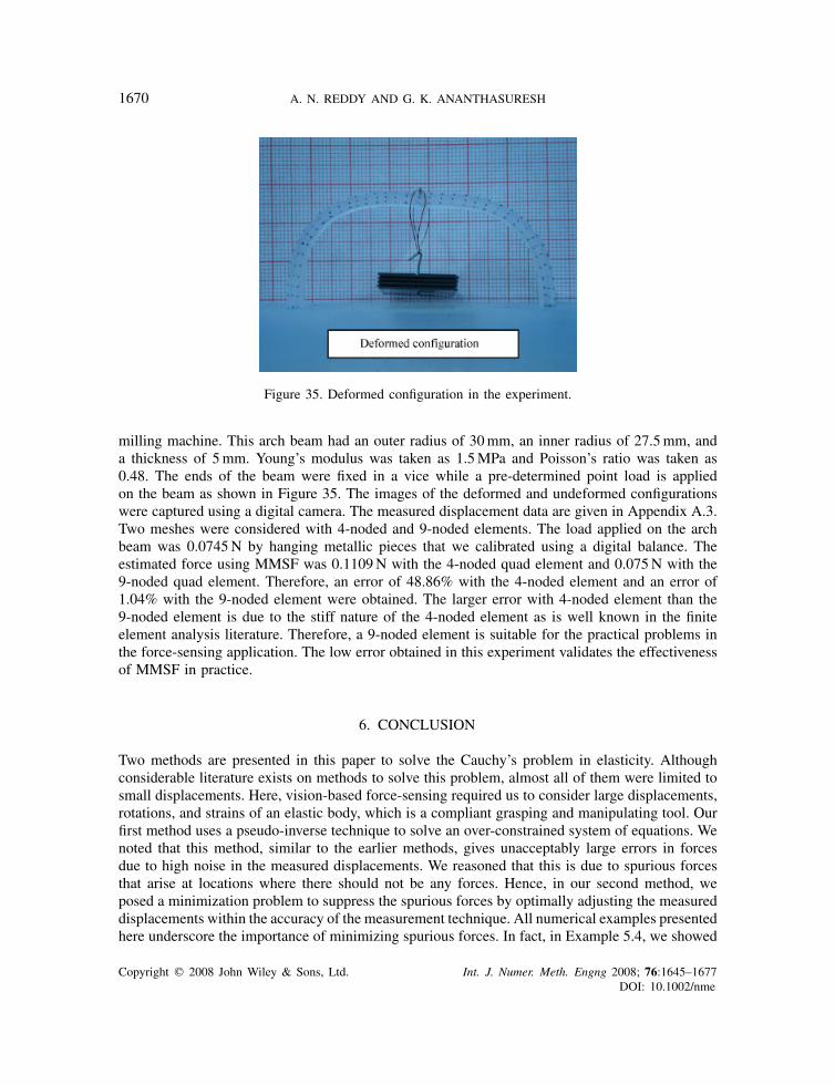
Figure 34. Undeformed configuration in the experiment.

The error in the estimated forces by DPIM is 1300.87% for 5% noise in the displacement data.However, MMSF brings the error in the estimated force to 29.55%, which gives the estimated forcein the same order of magnitude as the expected force as shown in Figure 33. The error of 29.55%is high. This may be because the horizontal (i.e. axial) stiffness of the beam is 1600 times largerthan the vertical (i.e. bending) stiffness. Such a case is known to be prone to increased error [1].

5.8. Example 8: experimental verification

Although the above numerical examples provided some insight into the methods, this last exampleis considered for validating the method with an experiment. We conducted the experiment on asilicone rubber arch beam as shown in Figure 34. It was vacuum-cast using a mould. The mouldfor this was made with a polypropylene sheet by using a computer numerically controlled (CNC)



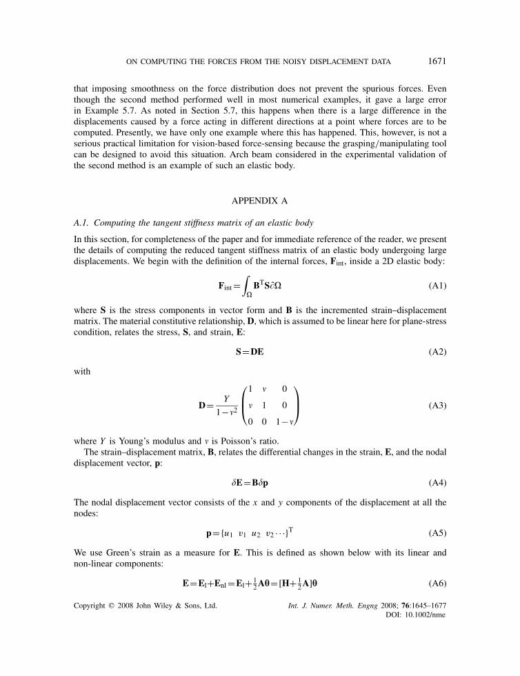
Figure 35. Deformed configuration in the experiment.

milling machine. This arch beam had an outer radius of 30mm, an inner radius of 27.5mm, anda thickness of 5mm. Young’s modulus was taken as 1.5MPa and Poisson’s ratio was taken as0.48. The ends of the beam were fixed in a vice while a pre-determined point load is appliedon the beam as shown in Figure 35. The images of the deformed and undeformed configurationswere captured using a digital camera. The measured displacement data are given in Appendix A.3.Two meshes were considered with 4-noded and 9-noded elements. The load applied on the archbeam was 0.0745N by hanging metallic pieces that we calibrated using a digital balance. Theestimated force using MMSF was 0.1109N with the 4-noded quad element and 0.075N with the9-noded quad element. Therefore, an error of 48.86% with the 4-noded element and an error of1.04% with the 9-noded element were obtained. The larger error with 4-noded element than the9-noded element is due to the stiff nature of the 4-noded element as is well known in the finiteelement analysis literature. Therefore, a 9-noded element is suitable for the practical problems inthe force-sensing application. The low error obtained in this experiment validates the effectivenessof MMSF in practice.

6. CONCLUSION

Two methods are presented in this paper to solve the Cauchy’s problem in elasticity. Althoughconsiderable literature exists on methods to solve this problem, almost all of them were limited tosmall displacements. Here, vision-based force-sensing required us to consider large displacements,rotations, and strains of an elastic body, which is a compliant grasping and manipulating tool. Ourfirst method uses a pseudo-inverse technique to solve an over-constrained system of equations. Wenoted that this method, similar to the earlier methods, gives unacceptably large errors in forcesdue to high noise in the measured displacements. We reasoned that this is due to spurious forcesthat arise at locations where there should not be any forces. Hence, in our second method, weposed a minimization problem to suppress the spurious forces by optimally adjusting the measureddisplacements within the accuracy of the measurement technique. All numerical examples presentedhere underscore the importance of minimizing spurious forces. In fact, in Example 5.4, we showed



that imposing smoothness on the force distribution does not prevent the spurious forces. Eventhough the second method performed well in most numerical examples, it gave a large errorin Example 5.7. As noted in Section 5.7, this happens when there is a large difference in thedisplacements caused by a force acting in different directions at a point where forces are to becomputed. Presently, we have only one example where this has happened. This, however, is not aserious practical limitation for vision-based force-sensing because the grasping/manipulating toolcan be designed to avoid this situation. Arch beam considered in the experimental validation ofthe second method is an example of such an elastic body.

APPENDIX A

A.1. Computing the tangent stiffness matrix of an elastic body

In this section, for completeness of the paper and for immediate reference of the reader, we presentthe details of computing the reduced tangent stiffness matrix of an elastic body undergoing largedisplacements. We begin with the definition of the internal forces, Fint, inside a 2D elastic body:

Fint=∫

BTS (A1)

where S is the stress components in vector form and B is the incremented strain–displacementmatrix. The material constitutive relationship, D, which is assumed to be linear here for plane-stresscondition, relates the stress, S, and strain, E:

S=DE (A2)

with

D= Y

1−2

⎛⎜⎝1 0

1 0

0 0 1−

⎞⎟⎠ (A3)

where Y is Young’s modulus and is Poisson’s ratio.The strain–displacement matrix, B, relates the differential changes in the strain, E, and the nodal

displacement vector, p:

E=Bp (A4)

The nodal displacement vector consists of the x and y components of the displacement at all thenodes:

p=u1 v1 u2 v2 · · ·T (A5)

We use Green’s strain as a measure for E. This is defined as shown below with its linear andnon-linear components:

E=El+Enl=El+ 12Ah=[H+ 1

2A]h (A6)



where A, h, and H are as follows:

A=

⎛⎜⎜⎜⎜⎜⎜⎜⎜⎜⎝

ux

0v

x0

0uy

0v

y

uy

ux

v

yv

x

⎞⎟⎟⎟⎟⎟⎟⎟⎟⎟⎠

, h=

ux

uy

v

xv

y

T

, H=

⎡⎢⎢⎣1 0 0 0

0 0 0 1

0 1 1 0

⎤⎥⎥⎦ (A7)

A differential change in E can be obtained as follows:

E=El+ 12Ah+ 1

2Ah+O(hTh)=El+Ah+O(hTh) (A8)

We note that

⎛⎜⎜⎜⎜⎜⎜⎜⎜⎜⎝

ux

0v

x0

0uy

0v

y

uy

ux

v

yv

x

⎞⎟⎟⎟⎟⎟⎟⎟⎟⎟⎠

⎧⎪⎪⎪⎪⎪⎪⎪⎪⎪⎪⎪⎪⎪⎪⎨⎪⎪⎪⎪⎪⎪⎪⎪⎪⎪⎪⎪⎪⎪⎩

u

x

u

y

v

x

v

y

⎫⎪⎪⎪⎪⎪⎪⎪⎪⎪⎪⎪⎪⎪⎪⎬⎪⎪⎪⎪⎪⎪⎪⎪⎪⎪⎪⎪⎪⎪⎭

=

⎛⎜⎜⎜⎜⎜⎜⎜⎜⎜⎝

u

x0

v

x0

0u

y0

v

y

u

yu

xv

yv

x

⎞⎟⎟⎟⎟⎟⎟⎟⎟⎟⎠

⎧⎪⎪⎪⎪⎪⎪⎪⎪⎪⎪⎪⎪⎪⎪⎨⎪⎪⎪⎪⎪⎪⎪⎪⎪⎪⎪⎪⎪⎪⎩

ux

uy

v

x

v

y

⎫⎪⎪⎪⎪⎪⎪⎪⎪⎪⎪⎪⎪⎪⎪⎬⎪⎪⎪⎪⎪⎪⎪⎪⎪⎪⎪⎪⎪⎪⎭

⇒ Ah=Ah (A9)

By neglecting the second- and higher-order terms in Equation (A8), we can re-write it as

E=[H+A]h (A10)

The x- and y-components of the displacements are now interpolated using shape functions andnodal displacement vector, p:

u = ∑iNiui

v = ∑iNivi

(A11)

where Ni ’s are the shape functions. This enables us to express h as follows:

h=Gp (A12)



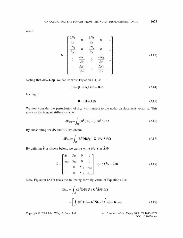
where

G=

⎡⎢⎢⎢⎢⎢⎢⎢⎢⎢⎢⎢⎢⎢⎣

N1

x0

N2

x0 . . .

N1

y0

N2

y0 . . .

0N1

x0

N2

x. . .

0N1

y0

N2

y. . .

⎤⎥⎥⎥⎥⎥⎥⎥⎥⎥⎥⎥⎥⎥⎦

(A13)

Noting that h=Gp, we can re-write Equation (11) as

E=[H+A]Gp=Bp (A14)

leading to

B=[H+A]G (A15)

We now consider the perturbation of Fint with respect to the nodal displacement vector, p. Thisgives us the tangent stiffness matrix:

Fint=∫

(BT(S)+(B)TS) (A16)

By substituting for S and B, we obtain

Fint=∫

(BTDBp+GTATS) (A17)

By defining S as shown below, we can re-write ATS as Sh:

S=

⎡⎢⎢⎢⎢⎣S11 S12 0 0

S12 S22 0 0

0 0 S11 S12

0 0 S12 S22

⎤⎥⎥⎥⎥⎦ ⇒ ATS= Sh (A18)

Now, Equation (A17) takes the following form by virtue of Equation (13):

Fint =∫

(BTDBU+GTSh)

=[∫

(BTDB+GTSG)

]p=KTp (A19)



200 400 600 800 1000 1200 1400 1600 1800 2000

– 1000

–900

– 800

–700

–600

– 500

– 400

–300

–200

–100

01 2 3

45

6 7 8 9 10 1112

1413

15

16

17

18

192021

2222

23

24

25

26

2728

29

30

31

32

33

34

35

36

37

383940

41 42

43 44

45

46

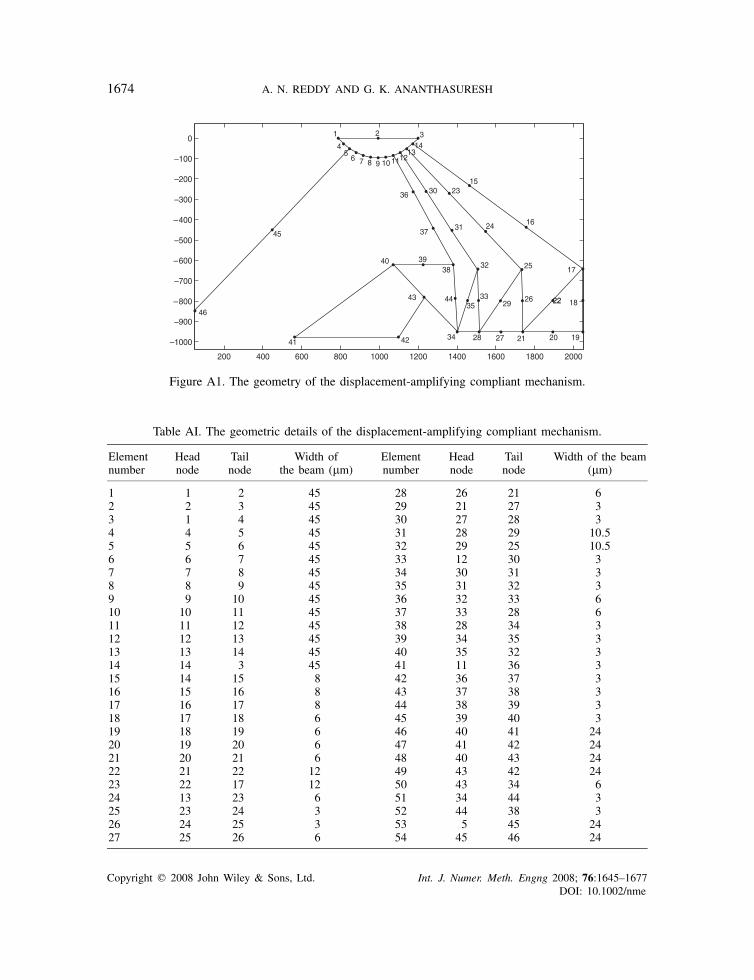
Figure A1. The geometry of the displacement-amplifying compliant mechanism.

Table AI. The geometric details of the displacement-amplifying compliant mechanism.

Element Head Tail Width of Element Head Tail Width of the beamnumber node node the beam (m) number node node (m)

1 1 2 45 28 26 21 62 2 3 45 29 21 27 33 1 4 45 30 27 28 34 4 5 45 31 28 29 10.55 5 6 45 32 29 25 10.56 6 7 45 33 12 30 37 7 8 45 34 30 31 38 8 9 45 35 31 32 39 9 10 45 36 32 33 610 10 11 45 37 33 28 611 11 12 45 38 28 34 312 12 13 45 39 34 35 313 13 14 45 40 35 32 314 14 3 45 41 11 36 315 14 15 8 42 36 37 316 15 16 8 43 37 38 317 16 17 8 44 38 39 318 17 18 6 45 39 40 319 18 19 6 46 40 41 2420 19 20 6 47 41 42 2421 20 21 6 48 40 43 2422 21 22 12 49 43 42 2423 22 17 12 50 43 34 624 13 23 6 51 34 44 325 23 24 3 52 44 38 326 24 25 3 53 5 45 2427 25 26 6 54 45 46 24



where the tangent stiffness matrix, KT, relating the change in the nodal displacement vector andthe change in the internal force vector is defined as follows with its linear and non-linear parts:

KT=KTl+KTnl=∫

(BTDB+GTSG)d (A20)

For further details regarding internal force and tangent stiffness matrix refer [29] or any book onnon-linear finite element methods. Similarly, co-rotational beam element formulation can also befound in [29]. The KT shown in the main body of the paper is the reduced stiffness matrix whereinthe specified zero displacements on fixed are applied.

A.2. The geometric details of the displacement-amplifying compliant mechanism

The geometric details of the displacement-amplifying compliant mechanism are given Figure A1and Table AI.

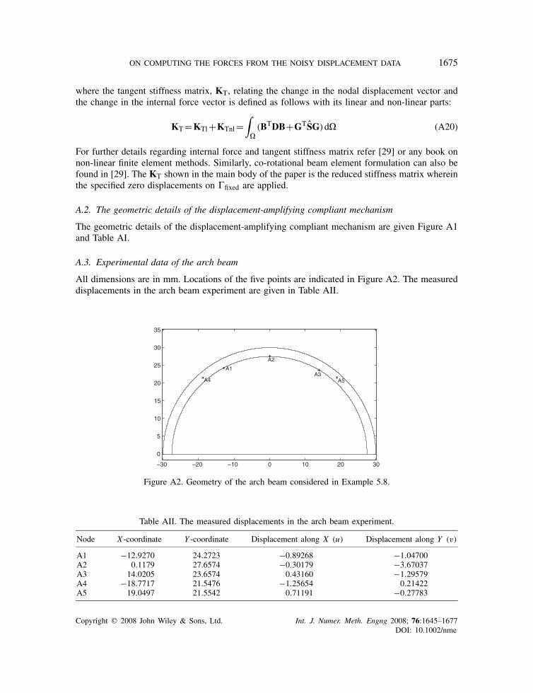
A.3. Experimental data of the arch beam

All dimensions are in mm. Locations of the five points are indicated in Figure A2. The measureddisplacements in the arch beam experiment are given in Table AII.

– 30 –20 –10 0 10 20 30

0

5

10

15

20

25

30

35

A1

A2

A3A4 A5

Figure A2. Geometry of the arch beam considered in Example 5.8.

Table AII. The measured displacements in the arch beam experiment.

Node X -coordinate Y -coordinate Displacement along X (u) Displacement along Y (v)

A1 −12.9270 24.2723 −0.89268 −1.04700A2 0.1179 27.6574 −0.30179 −3.67037A3 14.0205 23.6574 0.43160 −1.29579A4 −18.7717 21.5476 −1.25654 0.21422A5 19.0497 21.5542 0.71191 −0.27783



ACKNOWLEDGEMENTS

The authors would like to thank Sudarshan Hedge for helpful discussions; Sridhar (CPDM) and G. Balajifor their help in making the beam using vacuum casting and its mould on a CNC machine; NandanMaheswari for designing the gripper in Figure 1(a); Girish Krishnan for providing the geometry of thedisplacement-amplifying compliant mechanism; and Sivanagendra for providing geometric non-linear co-rotational beam element MATLAB code. The authors thank the department of Centre for Product Designand Manufacturing at the Indian Institute of Science, Bangalore, for providing vacuum casting and CNCmachining facilities. This work is supported in part by the Swarnajayanthi fellowship of the Departmentof Science and Technology, Government of India, to the second author.

REFERENCES

1. Wang X, Ananthasuresh GK, Ostrowski JP. Vision-based sensing of forces in elastic objects. Sensors andActuators A: Physical 2001; 94(3):142–156.

2. Greminger MA, Nelson BJ. Vision-based forces measurement. IEEE Transactions on Pattern Analysis andMachine Intelligence 2004; 26(3):290–298.

3. Kamiyama K, Vlack K, Mizota T, Kajimoto H, Kawakami N, Tachi S. Vision-based sensor for real time measuringof surface traction. IEEE Computer Graphics and Applications 2005; 25(1):68–75.

4. Vendroux G, Knauss WG. Submicron deformation field measurements. Part 2. Improved digital image correlation.Experimental Mechanics 1998; 38(2):86–92.

5. Charette PG, Hunter IW, Hunter PJ. Large deformation mechanical testing of biological membranes using speckleinterferometry in transmission. I: experimental apparatus. Applied Optics 1997; 36(10).

6. Zhang R, Shilo D, Ravichandran G, Bhattacharya K. Mechanical characterization of released thin films by contactloading. ASME Journal of Applied Mechanics 2006; 73:730–736.

7. Schnur DS, Zabaras N. Finite element solution of two-dimensional inverse elastic problems using spatialsmoothing. International Journal for Numerical Methods in Engineering 1990; 30(1):57–75.

8. Bonnet M, Constantinescu A. Inverse problems in elasticity. Inverse Problems 2005; 21:R1–R50.9. Tikhonov AN, Arsenin VY. Solution of Ill-posed Problems. V.H. Winston: Washington, DC, 1977.10. Belgacem FB. Why is the Cauchy problem severely ill-posed? Inverse Problems 2007; 23:823–826.11. Krishnan G, Ananthasuresh GK. An objective evaluation of displacement-amplifying compliant mechanisms

for sensor applications. CD-ROM Proceedings of the ASME International Design Engineering and TechnicalConferences, Philadelphia, U.S.A., 10–13 September 2006; Paper #DETC2006-99345 (Also to appear in theJournal of Mechanical Design 2008).

12. Oda J, Moto S. On inverse analytical technique to obtain contact stress distributions-technique using measurementvalues with errors (in Japanese but with an abstract in English). Transactions of the Japan Society of MechanicalEngineers, Series A 1980; 55:827–877.

13. Maniatty A, Zabaras N, Stelson K. Finite-element analysis of some inverse elasticity problems. Journal ofEngineering Mechanics (ASCE) 1989; 115(11):1303–1317.

14. Zabaras N, Morellas V, Schnur D. Spatially regularized solution of inverse elasticity problems using the BEM.Communications in Applied Numerical Methods 1989; 5(3):547–553.

15. Maniatty AM, Zabaras NJ. Investigation of regularization parameters and error estimating in inverse elasticityproblems. International Journal for Numerical Methods in Engineering 1994; 37(6):1039–1052.

16. Bezerra LM, Saigal S. Inverse boundary traction reconstruction with the BEM. International Journal of Solidsand Structures 1995; 32(10):1417–1431.

17. Martin TJ, Halderman JD, Dulikravich GS. An inverse method to finding unknown surface tractions anddeformations in elastostatics. Computers and Structures 1995; 56(5):825–835.

18. Zhang F, Kassab AJ, Nicholson DW. A 3-D traction reconstruction method using BEM and internal strain data.AIAA/ASME/ASCE/AHS/ASC Structures, Structural Dynamics, and Materials Conference and Exhibit, 38th, andAIAA/ASME/AHS Adaptive Structures Forum, Kissimmee, FL, U.S.A., 7–10 April 1997; 1873–1883.

19. Lu S, Rizzo FJ. A boundary element strategy for elastostatic inverse problems involving uncertain boundaryconditions. International Journal for Numerical Methods in Engineering 1999; 46:957–972.

20. Turco E. An effective algorithm for reconstructing boundary conditions in elastic solids. Computer Methods inApplied Mechanics and Engineering 2001; 190(29–30):3819–3829.



21. Nakagiri S, Suzuki K. Finite element interval analysis of external loads identified by displacement input withuncertainty. Computer Methods in Applied Mechanics and Engineering 1999; 168:63–72.

22. Turco E. Is the statistical approach suitable for identifying actions on structures? Computers and Structures 2005;83:2112–2120.

23. Marine L. A meshless method for solving the Cauchy problem three-dimensional elastostatics. Computers andMathematics with Applications 2005; 50:73–92.

24. Kozlov VA, Maz’ya VG, Fomin AV. An iterative method for solving the Cauchy problem for elliptic equations.Computational Mathematics and Mathematical Physics 1991; 31(1):45–52.

25. Baranger TN, Andrieux A. An optimization approach for the Cauchy problem in linear elasticity. Structural andMultidisciplinary Optimization 2008; 35:141–152.

26. Belgacem FB, Feikh HE. On Cauchy’s problem: I. A variational Steklov–Poincare theory. Inverse Problems 2005;21:1915–1936.

27. Azaıez M, Belgacem FB, Fekih HE. On Cauchy’s problem: II. Completion, regularization and approximation.Inverse Problems 2006; 22:1307–1336.

28. Howell LL. Compliant Mechanisms. Wiley: New York, 2001.29. Crisfield MA. Non-Linear Finite Element Analysis of Solids and Structures. Wiley: New York, 1997.


oncomputingtheforcesfromthenoisydisplacementdata ...suresh/journal/j49ijnmereddy.pdf · int. j....

Documents