introduction to the finite volumes method. application …caminos.udc.es/info/asignaturas/201/finite...
TRANSCRIPT
Introduction to the Finite Volumes Method.Application to the Shallow Water Equations.
Jaime Miguel Fe Marques

Contents
1 Preliminary considerations 31.1 Study of the movement of a fluid . . . . . . . . . . . . . . . . 31.2 Number of dimensions of the model . . . . . . . . . . . . . . . 41.3 Discretization techniques . . . . . . . . . . . . . . . . . . . . . 41.4 Systems of hyperbolic equations . . . . . . . . . . . . . . . . . 51.5 The Shallow Water Equations . . . . . . . . . . . . . . . . . . 5
2 One dimensional approach 72.1 Introduction . . . . . . . . . . . . . . . . . . . . . . . . . . . . 72.2 Conservative variables and conservation laws . . . . . . . . . . 72.3 The Riemann problem . . . . . . . . . . . . . . . . . . . . . . 92.4 Centered and non-centered discretization . . . . . . . . . . . . 112.5 Numerical diffusion or viscosity . . . . . . . . . . . . . . . . . 132.6 Conservative schemes. . . . . . . . . . . . . . . . . . . . . . . 14
2.6.1 Integral Form . . . . . . . . . . . . . . . . . . . . . . . 142.6.2 Numerical fluxes . . . . . . . . . . . . . . . . . . . . . 152.6.3 Convergence . . . . . . . . . . . . . . . . . . . . . . . . 162.6.4 Consistency condition . . . . . . . . . . . . . . . . . . 162.6.5 Stability condition . . . . . . . . . . . . . . . . . . . . 172.6.6 Conservative scheme . . . . . . . . . . . . . . . . . . . 172.6.7 Godunov Method for a scalar equation . . . . . . . . . 182.6.8 Rankine-Hugoniot jump condition . . . . . . . . . . . . 20
2.7 Hyperbolic linear systems . . . . . . . . . . . . . . . . . . . . 212.8 Non-centered schemes for linear systems . . . . . . . . . . . . 23
3 Two-dimensional flow equations 253.1 Types of flow. Turbulent flow . . . . . . . . . . . . . . . . . . 253.2 Average value and fluctuation . . . . . . . . . . . . . . . . . . 263.3 Navier-Stokes Equations . . . . . . . . . . . . . . . . . . . . . 263.4 Reynolds Equations in 3D . . . . . . . . . . . . . . . . . . . . 273.5 The Shallow Water equations . . . . . . . . . . . . . . . . . . 29
1

CONTENTS 2
4 Application to the 2D SWE 314.1 Types of finite volumes . . . . . . . . . . . . . . . . . . . . . . 31
4.1.1 Cell-type finite volumes . . . . . . . . . . . . . . . . . 314.1.2 Vertex-type finite volumes . . . . . . . . . . . . . . . . 324.1.3 Edge-type finite volumes . . . . . . . . . . . . . . . . . 32
4.2 Description of the finite volumes used . . . . . . . . . . . . . . 324.3 Terms considered in the equations . . . . . . . . . . . . . . . . 334.4 Integration and discretization . . . . . . . . . . . . . . . . . . 34
4.4.1 Discretization of the time derivative . . . . . . . . . . . 364.4.2 Integration of the flux and source terms . . . . . . . . 364.4.3 Definition of the discretized flux . . . . . . . . . . . . . 374.4.4 Definition of the discretized source . . . . . . . . . . . 394.4.5 Discretization of the boundary conditions . . . . . . . . 404.4.6 Obtaining of the time step . . . . . . . . . . . . . . . . 40
4.5 Algorithm . . . . . . . . . . . . . . . . . . . . . . . . . . . . . 41
5 Some results 425.1 Types of boundary conditions . . . . . . . . . . . . . . . . . . 425.2 One dimensional problems . . . . . . . . . . . . . . . . . . . . 42
5.2.1 Straight channel with slope and bottom friction . . . . 435.2.2 Channel with an obstacle on the bottom . . . . . . . . 465.2.3 Dam break . . . . . . . . . . . . . . . . . . . . . . . . 485.2.4 Dam break with reflection . . . . . . . . . . . . . . . . 49
5.3 Two dimensional problems . . . . . . . . . . . . . . . . . . . . 525.3.1 Partial Dam Break . . . . . . . . . . . . . . . . . . . . 525.3.2 Flow in a fishway . . . . . . . . . . . . . . . . . . . . . 55
References 61
Chapter 1
Preliminary considerations
1.1 Study of the movement of a fluid
The motion of a viscous fluid in three dimensions is described by the Navier-Stokes equations, a system of partial differential equations without analyticalsolution. When solving these equations numerically we may use differentapproaches. The most ambitious is the Direct Numerical Simulation thatsolves all fluid movements. In this case we need to use a mesh size at least asfine as the smallest eddies, which can lead, in a medium size problem, to anumber of computing nodes the order of 109. Moreover, the frequency of thefastest events can be about 104 Hz which imposes a time step of not morethan 10−4 s to treat it properly.
A second approach, less expensive, is to simulate only the large eddies(Large Eddy Simulation, LES) modeling the effect of those of smaller size,which cannot be solved with a given mesh. The process can be described as“filtering equations”, after which the velocity field contains only the largercomponents. This process introduces a stress terms representing the inter-action between the two scales of motion and have a dissipative effect. Tocalculate the effect of these stresses there are different models known in theliterature as SGS (subgrid scale models). The LES is based on the work ofSmagorinsky [24].
In engineering applications, there is usually no need to know all the de-tails of a flow, but only some properties: the discharge through a channel,the velocity distribution in a section or a substance concentration in a certainvolume. For these cases there is a third approach, far less expensive than theother two, that produces sufficiently accurate results: they are the Reynoldsequations, which are obtained by averaging in time the Navier-Stokes equa-tions (Reynolds Averaged Navier-Stokes, RANS). The time averaging of the
3

CHAPTER 1. PRELIMINARY CONSIDERATIONS 4
variables produce, similarly to the LES case, some terms called Reynoldsstresses. The effect of these stresses can be modeled by estimating a turbu-lent viscosity, for which a turbulence model is needed.
1.2 Number of dimensions of the model
These models take into account the motion of fluid particles in the three spa-tial directions. This is a suitable approach to represent the three-dimensionalreality, but the complexity of 3D models can be intractable even for relativelysimple domains.
On the opposite end are the 1D models. They are accurate enough forcertain phenomena, such as the movement of fluid in a pipe. The free surface,if it exists, is determined by the value of the variable depth (h). The equationsare greatly simplified, leading to significant savings in computation time. Theproblem is that, in most cases, these models do not represent adequately thereal problem, not permitting, for instance, taking into account the effect ofa change of direction or an asymmetrical section.
However, there are a number of phenomena in which fluid motion occursmainly in two dimensions, for example when the bottom slope is small andthe movement of the particles is substantially parallel to it. This makes the2D models an interesting option with considerable saving compared to 3D,and they allow an approximation to reality much greater than that achievedwith 1D models.
1.3 Discretization techniques
With regard to the spatial discretization, most of the models used in Com-putational Fluid Dynamics (CFD) use one of the three following techniques:finite differences, finite elements or finite volumes.
The Finite Difference Method is the oldest of the three, although its pop-ularity has declined, perhaps due to its lack of flexibility from the geometricpoint of view. It is usually applied to structured meshes. Its implementationis simple, so new numerical schemes can easily be developed (especially in1D) that can be generalized to several dimensions and used in finite volumeformulations.
The Finite Volume formulation is now widely used in computational fluiddynamics, being its use very common in the field of shallow water equations[3] and 3D models [33]. It is applied to both structured and unstructuredmeshes with different shapes of the volumes. Its flexibility and conceptual

CHAPTER 1. PRELIMINARY CONSIDERATIONS 5
simplicity explain the acceptance it has. It has been used in commercialprograms [11]. In one dimension it is equivalent to the Finite DifferenceMethod and, depending on the mesh used and the type of discretization, itcan also be so with a higher number of dimensions.
The main advantage of the Finite Element Method stems from its rigor-ous mathematical foundation that allows a posteriori error estimation. It isconceptually more difficult than the Finite Volume Method and the physicalmeaning of the proceedings is less easily seen than in this, although its flexi-bility to adapt to any geometry is similar. It is used by different authors andapplied to commercial programs [6].
Some works [19, 35] compare both methods, showing that the Finite Vol-ume Method shares the theoretical basis of the Finite Element Method, sinceit is a particular case of the Weighted Residuals Formulation. However, theweighting used in the first (constant volumes in the case of first order ap-proximation) allows to take advantage of some properties of conservation,and the resolution algorithms are posed in a very advantageous way.
1.4 Systems of hyperbolic equations
Hyperbolic equations systems have been studied by a number of authorsover the last decades. In a first phase, the studies focused on homogeneoussystems but, since the 80s, more interest has been put in problems withsource term, which have more practical applications.
The applications were initially oriented to compressible fluids, achievingsignificant results in aerodynamics. The strong analogy between the equa-tions of compressible and incompressible flows have permitted to apply sim-ilar techniques to the shallow water equations, e.g. Glaister [14] using finitedifferences, or Vazquez Cendon [31], with finite volumes. Donea and Huerta[12] apply the Finite Element Method, in permanent and non-permanentproblems, both to compressible and incompressible fluids.
1.5 The Shallow Water Equations
The behavior of a viscous fluid is governed by the Navier Stokes equations.These equations were derived in 1821 by Claude Navier and, independently,by George Stokes in 1845. They form a hyperbolic system of nonlinear con-servation laws and, due to their complexity, have no analytical solution. Forthis reason, the 2D system of Shallow Water (or Saint Venant) Equationshas been obtained from them, by imposing several simplifying assumptions.
CHAPTER 1. PRELIMINARY CONSIDERATIONS 6
These equations describe the behavior of a fluid in shallow areas. Despitethe strong assumptions used in their obtaining, the results are very close toreality, even in cases where some of these hypotheses are not fulfilled. Someof the the many problems that can be solved are flow in channels and rivers,tidal flows, sea currents or progression of shockwaves. The one-dimensionalversion of these equations is commonly used in the study of flow in openchannels.
Despite its considerable simplicity compared to the Navier Stokes equa-tions, even 1D Saint Venant equations have no analytical solution and mustbe solved by approximate methods. The increase, in recent decades, of thecomputer power has allowed an increasing use of the two-dimensional shallowwater equations.
Since the 70s of last century, the Finite Element Method has begun tobe applied to the shallow water equations: Zienkiewicz [34], and Peraire [22]are among the authors who have worked on this line.
In parallel to this, the use of the Finite Volume method has grown: see,for instance, the worlks of Vazquez Cendon [31] and Alcrudo and Garcia-Navarro [2] among many others.
The calculation of the velocity field in a given domain permits the studyof many problems of practical interest, such as the sediment transport, theevolution of the salt concentration in an estuary or the dispersal of pollutants.
Chapter 2
One dimensional approach
2.1 Introduction
The aim of this chapter is to show the main aspects of the method in onespatial dimension. First, several commonly used terms are defined and somebasic concepts in numerical modeling are introduced or reminded. To de-scribe some of the techniques, simple equations in 1D are used, such as thetransport equation. In order to facilitate the application of the method tothe particular case of the shallow water equations, the final chapter definessome terms commonly used in open channels hydraulics.
2.2 Conservative variables and conservation
laws
Conservative variables. There is some freedom to choose the variablesthat describe the flow to study. One possible choice is to take the “primitive”or “physical” variables: the density ρ, the pressure p and the three compo-nents of velocity, u, v, w. Another one is to use the so-called “ conservative”variables, which result from applying the fundamental laws of conservation(of mass, momentum, energy). These variables are, for example: the threecomponents of momentum per unit volume ρu, ρv, ρw and the total energyper unit volume. For systems of equations governing the free surface flow inone or two dimensions, such as the Shallow Water system, the conservativevariables commonly used are the depth h and its product by the velocitycomponents: hu in one dimension and (hu, hv) in the two-dimensional case.
Conservation laws. They are systems of partial differential equationsexpressing conservation of m quantities u1, . . . um. If obtained from a control
7

CHAPTER 2. ONE DIMENSIONAL APPROACH 8
volume fixed in space, which is crossed by the moving fluid, they are saidto be written in conservative form, this is the way that most resembles aflow balance of mass and momentum [7, pg. 19]. If the control volume moveswith the fluid, so always contains the same particles, the non conservativeform is obtained [4, pg. 16]. A conservation law in conservative form iswritten
Ut + Fx = 0, U = U(x, t), F = F(U). (2.1)
U is called Variables Vector and F(U) Flux Functions Vector. When ex-pressing the conservation laws in differential form, it is assumed that thesolutions satisfy the relevant requirements of regularity.
Example 1 (scalar): The Transport equation (linear advection equation).
∂u
∂t+∂f
∂x= 0 u = u(x, t), f(u) = au, a = constant. (2.2)
Example 2 (scalar): Burgers equation.
∂u
∂t+∂f
∂x= 0 u = u(x, t), f(u) =
1
2u2. (2.3)
Example 3 (system of conservation laws): the one-dimensional shallowwater equations.
U =
{hhu
}, F(U) =
{hu
hu2 + 12gh
2
}. (2.4)
Nonconservative Form. If, for instance, we replace f by its value in theBurgers Equation we obtain the nonconservative form
∂u
∂t+ u
∂u
∂x= 0 u = u(x, t). (2.5)
If instead of an equation we consider a system of conservation laws, applyingthe chain rule we obtain the following expression:
∂U
∂t+
dF
dU
∂U
∂x=∂U
∂t+ A
∂U
∂x= 0 (2.6)
where A is the Jacobian matrix
A =dF
dU=
∂f1
∂u1. . .
∂f1
∂um...
. . ....
∂fm∂u1
· · · ∂fm∂um
. (2.7)
CHAPTER 2. ONE DIMENSIONAL APPROACH 9
The nonconservative formulation (2.6) is equivalent to the conservative one(2.1), and has the same solution, provided that this solution is sufficientlyregular. Otherwise the derivation which led to (2.6) is not valid. For example,if the solution is discontinuous –e.g. a shock wave– erroneous results areobtained.
Integral Form. The conservation laws can also be expressed in inte-gral form. One reason for the use of this form is that the obtaining of theequations is based on physical conservation principles, generally expressed asintegral relationships. On the other hand the integral formulation requiresless derivability conditions on solutions, which allows to obtain discontinuoussolutions. These discontinuous solutions do not verify the partial differen-tial equation at every point because the derivatives are not defined at thediscontinuities, and must meet a “jump condition” along them, which is ob-tained from the integral form (see 2.6.8, Rankine-Hugoniot condition). Thesolutions of the integral form are known as weak solutions.
2.3 The Riemann problem
We will analyze the Riemann problem for the importance it has on the Go-dunov method, from which the method that is described here derives.
The transport equation, already mentioned, has the form
∂u
∂t+ a
∂u
∂x= 0 u = u(x, t), a = constante. (2.8)
The Cauchy problem, applied to this equation consist in solving it withthe initial condition
u(x, 0) = u0(x). (2.9)
As it can easily be seen by substituting in the equation, the solution is givenby
u(x, t) = u0(x− at), ∀x ∈ R, ∀t ≥ 0, (2.10)
which can be interpreted saying that the function u moves in time, along theaxis x, speed a without deforming.
The points of the plane x, t in which the above said occurs are calledcharacteristic curves. Their equation in this case is given by
dx
dt= a
(in general,
dx
dt= f ′(u)
)(2.11)
and in them the solution u of the equation remains constant. Indeed, if u isa solution of the equation, the total derivative satisfies
du
dt=∂u
∂t+∂u
∂x
dx
dt=∂u
∂t+ a
∂u
∂x= 0. (2.12)
CHAPTER 2. ONE DIMENSIONAL APPROACH 10
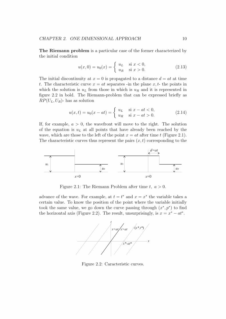
The Riemann problem is a particular case of the former characterized bythe initial condition
u(x, 0) = u0(x) =
{uL si x < 0,uR si x > 0.
(2.13)
The initial discontinuity at x = 0 is propagated to a distance d = at at timet. The characteristic curve x = at separates -in the plane x, t- the points inwhich the solution is uL from those in which is uR and it is represented infigure 2.2 in bold. The Riemann-problem that can be expressed briefly asRP (UL, UR)- has as solution
u(x, t) = u0(x− at) =
{uL si x− at < 0,uR si x− at > 0.
(2.14)
If, for example, a > 0, the wavefront will move to the right. The solutionof the equation is uL at all points that have already been reached by thewave, which are those to the left of the point x = at after time t (Figure 2.1).The characteristic curves thus represent the pairs (x, t) corresponding to the
( )x*,t*
x*-at*x
t
uL
uR
x=0
uR
x=0
d=at
uL
Figure 2.1: The Riemann Problem after time t, a > 0.
advance of the wave. For example, at t = t∗ and x = x∗ the variable takes acertain value. To know the position of the point where the variable initiallytook the same value, we go down the curve passing through (x∗, p∗) to findthe horizontal axis (Figure 2.2). The result, unsurprisingly, is x = x∗− at∗.
uL
uR
x=0
uR
x=0
d=at
uL
( )x*,t*
x*-at*x
t
x>atx<at
Figure 2.2: Caracteristic curves.
CHAPTER 2. ONE DIMENSIONAL APPROACH 11
2.4 Centered and non-centered discretization
Before describing the finite volume method (section 2.6) and applying it tothe shallow water equations (chapter 4), we apply the centered and non-centered discretization to the Transport Equation.
Equation (2.8) is considered again
∂u
∂t+ a
∂u
∂x= 0 u = u(x, t), a = constant. (2.15)
Different discretizations for this equation can be obtained from the Taylorseries expansion. For example, if i is the spatial index and n the time index,
un+1i = uni +
∂u
∂t
∣∣∣ni4t+
1
2
∂2u
∂t2
∣∣∣ni4t2 +O(4t3) (2.16)
and the time derivative can be approximated as
∂u
∂t
∣∣∣ni
=un+1i − uni4t
− 1
2
∂2u
∂t2
∣∣∣ni4t+O(4t2), (2.17)
which is a first order forward discretization. Also
uni+1 = uni +∂u
∂x
∣∣∣ni4x+
1
2
∂2u
∂x2
∣∣∣ni4x2 +
1
6
∂3u
∂x3
∣∣∣ni4x3 +O(4x4), (2.18)
uni−1 = uni −∂u
∂x
∣∣∣ni4x+
1
2
∂2u
∂x2
∣∣∣ni4x2 − 1
6
∂3u
∂x3
∣∣∣ni4x3 +O(4x4), (2.19)
and subtracting these two equations, we obtain a space centered second orderdiscretization
∂u
∂x
∣∣∣ni
=uni+1 − uni−1
24x− 1
6
∂3u
∂x3
∣∣∣ni4x2 +O(4x3). (2.20)
Then equation (2.15) can be written in discretized form as
un+1i − uni4t
+ auni+1 − uni−1
24x= 0 (2.21)
from which the following numerical algorithm results
un+1i = uni −
1
2
a4t4x
(uni+1 − uni−1). (2.22)
This scheme, first order in time and second in space is called Euler explicitscheme and it can be shown that is unconditionally unstable [27, pg. 163].
CHAPTER 2. ONE DIMENSIONAL APPROACH 12
In order to remedy the lack of stability observed in the above scheme, wediscretize spatially in non-centered form, which produces two options
∂u
∂x
∣∣∣ni
=uni − uni−1
4x, (2.23)
∂u
∂x
∣∣∣ni
=uni+1 − uni4x
, (2.24)
from which only one is successful, depending on the sign of the speed a ofthe wave. If a > 0, the option (2.23) together with (2.17) results
un+1i − uni4t
+ auni − uni−1
4x= 0 (2.25)
from whereun+1i = uni − c(uni − uni−1), (2.26)
being
c =a4t4x
, (2.27)
This scheme proves to be stable [27, pg. 164] provided that
0 ≤ c ≤ 1. (2.28)
The parameter c is called the Courant number or the CFL (Courant-Friedrichs-Lewy) number. It can be considered as the ratio of two lengths:the one traveled by the wave in time 4t and the mesh size 4x. As a is adatum and 4x is usually determined by the desired degree of accuracy, onecan only vary 4t to satisfy the stability condition.
The scheme (2.26) is known as the first order upwind scheme and alsothe CIR scheme, (Courant, Isaacson and Rees). The name upwind refers tothe fact that in the spatial discretization we use grid points from the sidewhere information comes. The CIR has the disadvantage, common to all firstorder methods of being very diffusive: it tends to smooth discontinuities inthe solution and cut extreme values.
If, for a > 0, we introduce (2.17) and (2.24) in the transport equation(2.15), the resulting downwind scheme
un+1i = uni − c(uni+1 − uni ), (2.29)
is unconditionally unstable. That is, to obtain a useful non-centered schemethe sign of a in the spatial discretization must be taken into account.
CHAPTER 2. ONE DIMENSIONAL APPROACH 13
Another first order scheme is the Lax-Friedrichs, characterized for re-placing the term uni in (2.22) by
1
2(uni−1 + uni+1), (2.30)
i.e. the average of the values in the two neighboring nodes. The resultingscheme
un+1i =
1
2(1 + c)uni−1 +
1
2(1− c)uni+1 (2.31)
is stable under the condition (2.28) [27, pg. 168].
2.5 Numerical diffusion or viscosity
We will try to clarify below the previous section assertion that the first orderschemes are diffusive. Let us consider Equation (2.8) without time derivative
a∂u
∂x= 0, a > 0. (2.32)
If the non-centered discretization (2.23) is applied, we get
a∂u
∂x
∣∣∣i
= aui − ui−1
4x+O(4x). (2.33)
Moreover, from the Taylor series expansion (2.19),
ui−1 = ui −∂u
∂x
∣∣∣i4x+
1
2
∂2u
∂x2
∣∣∣i4x2 +O(4x3), (2.34)
whence, multiplying by a and rearranging, we obtain
a∂u
∂x
∣∣∣i− 1
2a4x∂
2u
∂x2
∣∣∣i
= aui − ui−1
4x+O(4x2). (2.35)
That is, the expression
aui − ui−1
4x, (2.36)
which represents a first order discretization of (2.32), is simultaneously asecond order discretization (thus more accurate) of
a∂u
∂x− a4x
2
∂2u
∂x2 = 0, (2.37)
containing a diffusive term with a coefficient a4x/2.
CHAPTER 2. ONE DIMENSIONAL APPROACH 14
So when discretizing upwind Equation (2.32) a so-called numerical dif-fusion is being introduced. The coefficient that quantifies this diffusion (alsocalled numerical viscosity) depends on the mesh size, so if4x is sufficientlysmall, thereby increasing the computation time, the diffusive effect tends todisappear. If, however, the diffusive effect is high, the extreme values of thesolution tend to cut and discontinuities to spread.
Another solution to reduce the diffusive effect is to use higher orderschemes. These schemes take into consideration the values in a larger numberof nodes, so the programming is more complicated. Lowering the numericalviscosity also reduces stability.
2.6 Conservative schemes.
The finite volume method in one spatial dimension is based on dividing thespatial domain into intervals (called finite volumes or cells) making in eachof them an approximation of the integral of the conservative variables. Ateach time step these values are updated using approximations of the fluxat the ends of the intervals, as it will be discussed below, using the scalarconservation law
∂u
∂t+∂f
∂x= 0, u = u(x, t), f = f(u), (2.38)
that represents the transport equation if f(u) = au, being a a constant.
2.6.1 Integral Form
A way to discretize (2.38), considering weak solutions, is to divide the spatialdomain into finite volumes and integrate the equation in each cell, trans-forming it into an integral form. For simplicity, we will use intervals (finitevolumes) with equal length 4x and take a constant time step 4t. Thus thespatial and temporal domains will be
Ii =[xi− 1
2, xi+ 1
2
]=[xi − 4x2 , xi +
4x2
],
In = [tn, tn+1] = [n4t, (n+ 1)4t](2.39)
and the integral in the cell, of Equation (2.38)∫ xi+1
2
xi− 1
2
[∂u
∂t+∂f
∂x
]dx = 0, (2.40)

CHAPTER 2. ONE DIMENSIONAL APPROACH 15
becomes ∫ xi+1
2
xi− 1
2
∂u
∂tdx+ f(u(xi+ 1
2, t))− f(u(xi− 1
2, t)) = 0. (2.41)
Since the interval ends xi± 12
do not depend on time, we can write
∂
∂t
∫ xi+1
2
xi− 1
2
u(x, t)dx+ f(u(xi+ 12, t))− f(u(xi− 1
2, t)) = 0. (2.42)
We define uni as the spatial average of the function u(x, t) in the interval Ii,at time tn = n4t, i.e.
uni =1
4x
∫ xi+1
2
xi− 1
2
u(x, tn)dx, (2.43)
Integrating (2.42) between tn and tn+1, the time derivative disappears fromthe first term, resulting∫ x
i+12
xi− 1
2
[u(x, tn+1)− u(x, tn)] dx
+
∫ tn+1
tn
[f(u(xi+ 1
2, t))− f(u(xi− 1
2, t))]dt = 0 (2.44)
and we see that the value of u in Ii only changes along time 4t dueto the value of the flux f at the ends of Ii. Then, using (2.43),(
un+1i − uni
)4x+
∫ tn+1
tn
[f(u(xi+ 1
2, t))− f(u(xi− 1
2, t))]dt = 0. (2.45)
2.6.2 Numerical fluxes
In the above expression, the values of the integral of f at points xi± 12
willnot be generally known, so we replace them with
fni± 1
2≈ 1
4t
∫ tn+1
tn
f(u(xi± 12, t))dt, (2.46)
so we get
un+1i = uni −
4t4x
(fni+ 1
2− fn
i− 12
). (2.47)
The explicit algorithm (2.47) allows us to obtain the approximation of u ineach cell, at time tn+1, from its value in the previous time and the numericalfluxes fn
i± 12
at the ends of the cell.

CHAPTER 2. ONE DIMENSIONAL APPROACH 16
These numerical fluxes represent approximations of the time average ofthe physical flux at the edges of the cell and, depending on the waythey are calculated, we get different schemes. To calculate them, thevariables in cells adjacent to Ii are used
fni± 1
2= φ(uni−m, u
ni−m+1, . . . , u
ni+l), (2.48)
where m and l are two non-negative integers and φ is a certain function.In hyperbolic problems information propagates at a finite speed, so it
seems reasonable to assume that we can obtain fni− 1
2
from uni−1 and uni (the
average values of the variable on both sides of the boundary xi− 12), while
fi+ 12n
is obtained from uni and uni+1. Then the general expression (2.48) takesthe form
fni− 1
2= φ(uni−1, u
ni ) ; fn
i+ 12
= φ(uni , uni+1). (2.49)
2.6.3 Convergence
The algorithm (2.47) allows us to obtain variable values forward in time. Toprovide a good approximation of the law of conservation, the algorithm mustbe convergent. which means that the numerical solution converges to thesolution of the differential equation when 4x,4t→ 0.
Convergence is ensured with two requirements: consistency and stabil-ity. Indeed, Lax Theorem states that a consistent and stable scheme isconvergent. We will briefly discuss both.
2.6.4 Consistency condition
We say that a scheme is consistent if it represents faithfully the differentialequation when 4t→ 0, 4x→ 0. As we are getting the numerical flux fromthe values of u in neighboring cells, if u has the same value in all of them,the result must be the same in each one. Therefore, a consistency conditionrequired to function φ is:
φ(v, v, . . . , v) = f(v); (2.50)
Usually, continuity for the variable u is also required, i.e. φ(uni−1uni )→ f(v),
when uni−1, uni → v [20, pg. 68].
CHAPTER 2. ONE DIMENSIONAL APPROACH 17
2.6.5 Stability condition
A method must be stable in the sense that a small error introduced at anytime step is not amplified indefinitely but remains bounded along the process.In paragraph 2.4 it was said that the Euler explicit scheme was uncondition-ally unstable, while the CIR scheme was stable when 0 ≤ c ≤ 1. Thesestatements are based on the stability criterion of Von Neumann, which isbased on Fourier analysis and is very useful in the study of linear systems.
2.6.6 Conservative scheme
A conservative scheme for the scalar conservation law (2.38) is a numericalmethod of the form (2.47) that fulfills the condition (2.48).
We see that by applying a conservative scheme to a set of contiguouscells N,N + 1 . . .M , the result verifies the same property (2.44) of the exactsolution (the value of u in Ii only changes in time 4t due to the value of theflow f at the ends of Ii). Indeed, adding the values of un+1
i obtained from(2.47), for any set of consecutive cells, multiplying by 4x and rearranging,we get (
M∑i=N
un+1i −
M∑i=N
uni
)4x+
(fnM+ 1
2− fn
N− 12
)4t = 0, (2.51)
since fluxes at cell boundaries cancel each other, except for flows at the endsx = xN− 1
2and x = xM+ 1
2.
The interest of conservative schemes is that, as the Theorem of Lax-Wendroff [15, pg. 168] says, if a consistent conservative scheme converges,the result is a weak solution of the equation. In contrast, non-conservativeschemes may not converge to the correct solution, if a shock wave is present[27, pg. 170]. Two examples of conservative schemes are the Godunov andLax-Friedrichs schemes.
We may say that the Lax-Wendroff theorem “continues” Lax’s Theorem.That is, a scheme consistent, stable and conservative converges at a weaksolution of the equation.
The algorithm (2.47) can also be seen as a finite difference approximationof the conservation law (2.38), as this law can be discretized as
un+1i − uni4t
+fni+ 1
2− fn
i− 12
4x= 0, (2.52)
where fni+ 1
2
, fni− 1
2
are approximations of the value of f at the endpoints.
CHAPTER 2. ONE DIMENSIONAL APPROACH 18
2.6.7 Godunov Method for a scalar equation
Godunov conducted the first conservative extension of the CIR scheme tononlinear systems of conservation laws. The Godunov first order upwindmethod is a conservative scheme in the form (2.47), where the numericalfluxes at the boundaries of the cells, fi± 1
2, are calculated using solutions
of local Riemann problems. It means that a Riemann Problem is solvedin every time step at every boundary between two cells, taking as initialvalues at each side of the boundary, the average values of the variable in theprevious time step, as discussed below.
It is assumed that in each time step tn, variable u is piecewise constant,taking on each cell Ii the value given by (2.43). There are, then, a pair ofsteady states at each boundary of Ii : (ui−1, ui) on the left and (ui, ui+1)on the right, both of which can be considered as a local Riemann Problem,originating at x = 0, t = 0. Thus, in the left side, x = xi− 1
2, we have
∂u∂t
+∂f∂x
= 0,
u(x, 0) = u0(x) =
{uni−1, x < 0,uni , x > 0,
(2.53)
and, on the right side, x = xi+ 12,
∂u∂t
+∂f∂x
= 0,
u(x, 0) = u0(x) =
{uni , x < 0,uni+1, x > 0.
(2.54)
Let u(x, t) be the combined solution of RP (uni−1, uni ) and RP (uni , u
ni+1)
in Ii. Since u(x, t) is the exact solution of the conservation law (2.38), weintroduce it in the integral form (2.44), with spatial and temporal domains,respectively
Ii = [xi− 12, xi+ 1
2], In = [0,4t] , (2.55)
obtaining∫ xi+1
2
xi− 1
2
u(x,4t)dx =
∫ xi+1
2
xi− 1
2
u(x, 0)dx
−∫ 4t
0
f(u(xi+ 12, t))dt+
∫ 4t
0
f(u(xi− 12, t))dt = 0. (2.56)

CHAPTER 2. ONE DIMENSIONAL APPROACH 19
Now we define, as in (2.43)
uni = 14x
∫ xi+1
2
xi− 1
2
u(x, 0)dx,
un+1i = 1
4x
∫ xi+1
2
xi− 1
2
u(x,4t)dx,
(2.57)
and it results the conservative scheme (2.47)
un+1i = uni −
4t4x
(fni+ 1
2− fn
i− 12
), (2.58)
being
fi± 12
=1
4t
∫ 4t
0
f(u(xi± 12, t))dt. (2.59)
The integrand in (2.59) depends on the exact solution to the Riemann Prob-lem, at each end of the cell, along the time axis (in local coordinates, thenat x = 0). This is represented as
u(xi± 12, t) = ui± 1
2(0), (2.60)
wherebyfi± 1
2= f(ui± 1
2(0)). (2.61)
If, for instance, the flux function is f(u) = au, a > 0, it results
fi− 12
= auni−1, fi+ 12
= auni (2.62)
(if, instead, we take a < 0 the result is auni on the left boundary and auni+1
on the right). Replacing in (2.58), we arrive at
un+1i = uni +
4t4x
(auni−1 − auni ) = uni −a4t4x
(uni − uni−1), (2.63)
i.e. the CIR scheme (2.26).Thus, Godunov Method considers the problem to be solved as a suc-
cession of states, constant in each finite volume. At each time step aRiemann problem at the boundary of each cell is solved, taking the exactsolutions of each local problem as the fluxes in these boundaries. Theseexact solutions must be calculated according to the equation in question, ifit is not linear; in [27, pg.176], the exact solutions of Riemann problem in the
CHAPTER 2. ONE DIMENSIONAL APPROACH 20
case of the quasi-linear Burgers equation may be seen. Finally, the spatialaveraging of the dependent variables in each cell is performed.
To simplify the process, different authors [16, 23, 30] have used schemescalled approximate Riemann solvers, which they have applied to com-pressible fluids. These schemes have been extended later [2, 14, 29, 31] to freesurface flows with very good results (in [20] different approximate Riemannsolvers are described). While it is true that these schemes will replace theexact solution of the Riemann problem by an approximate one, the infor-mation provided by the exact solution is partially lost in any case, due tospatial averaging in each cell, which makes less significant the error in theapproximation [8].
In the conservative scheme of Lax-Friedrichs the fluxes at the ends arecalculated as
fi+ 12
= 1 + c2c f(uni ) + c− 1
2c f(uni+1),
fi− 12
= 1 + c2c f(uni−1) + c− 1
2c f(uni ),
(2.64)
where c takes the value given by (2.27). If f(u) = au and we replace (2.64)in equation (2.47), the finite differences scheme (2.31) of Lax-Friedrichs isobtained.
2.6.8 Rankine-Hugoniot jump condition
In the preceding description of Godunov’s Method, the integral form is dis-cretized, looking for weak solutions to the differential equation (2.38), whenthe initial condition is discontinuous (Riemann problem).
Of course, any function u that is a “classical” solution (hence differen-tiable) of the equation will be a weak solution. And a weak solution is a“classical” solution in the intervals in which it is differentiable.
In the event that there is a discontinuity in a weak solution u(x, t), thefunction will take values uL and uR at both sides of the discontinuity. Thenthe following relationship, known as the Rankine-Hugoniot condition, is ver-ified,
(uR − uL)S = f(uR)− f(uL) (2.65)
being S the speed at which the jump is transmitted.The Rankine-Hugoniot condition is shown in [27, pg. 70], using the Leib-
nitz formula and in [20, pg. 212] based on geometrical considerations. In thefollowing examples we obtain this velocity S in two cases.
Example 1. The transport equation, where f(u) = au, a constant.
S =f(uR)− f(uL)
uR − uL=auR − auLuR − uL
= a. (2.66)
CHAPTER 2. ONE DIMENSIONAL APPROACH 21
As we already knew (2.3), the wave moves at a constant speed a.
Example 2. Burgers equation. Now f(u) = 12u
2.
S =
1
2u2R −
1
2u2L
uR − uL=uR + uL
2. (2.67)
In this case, the speed of advance of the wave depends on the values of u atboth sides of the discontinuity.
2.7 Hyperbolic linear systems
In paragraphs 2.4 to 2.6 we have referred to the case of a partial differentialequation. Conservation laws are usually given in the form of a system ofnonlinear equations. We will describe some techniques, for the case of linearsystems, which can be extended to nonlinear systems.
Let a linear system of partial differential equations
Ut + AUx = 0, U = {uj}, j = 1, 2 . . .m, (2.68)
where U is the variables vector and Am×m a constant matrix. The systemis called hyperbolic if A is diagonalizable, i.e. if it has m real eigenvaluesλi and m eigenvectors linearly independent ki. It is strictly hyperbolic if allthe eigenvalues are different.
Calling Λ the diagonal matrix of eigenvalues and X the matrix whosecolumns are the eigenvectors ki, it holds
A = XΛX−1. (2.69)
The existence of X−1 allows us to define a new vector of variables
V = {vj}j=1,2...m = X−1U. (2.70)
Using the relationships (2.69) and U = XV it results, from (2.68),
XVt + XΛX−1XVx = XVt + XΛVx = X (Vt + ΛVx) = 0, (2.71)
from whereVt + ΛVx = 0. (2.72)
Thus the system in canonical or characteristic form has been obtained.Each of the resulting m uncoupled equations have only one variable involved
∂vj∂t
+ λj∂vj∂x
= 0 j = 1, 2 . . .m, (2.73)

CHAPTER 2. ONE DIMENSIONAL APPROACH 22
and take the form of the 1D transport equation. Thus, the system can be seenas a combination of m waves traveling at their characteristic velocitiesgiven by the m eigenvalues λj. These eigenvalues (or characteristic values)define the characteristic curves x(t) = x0 + λjt, (see 2.3, along which theinformation corresponding to each one of the characteristic variables {vj}propagates.
With the above said we have made a basis change to the set of eigenvectorski. The characteristic variables can be interpreted then as the componentsof the variables vector U in the reference system formed by the eigenvectors(being X−1 the basis change matrix) or, what is the same, as the projectionsof the vector U on the eigenvectors.
After solving the system (2.73), the values U can be obtained from therelationship (2.70). For example, let us consider the system
Ut + Fx = 0, U =
{u1
u2
}, F =
{2u1
u1 + u2
}(2.74)
which, by applying the rule of the chain, changes to
Ut + AUx = 0, U =
{u1
u2
}, A =
{2 01 1
}. (2.75)
From matrix A we obtain
λ1 = 2, λ2 = 1, X =
{1 01 1
}, X−1 =
{1 0−1 1
}. (2.76)
Then, using the base change (2.70), the characteristic variables are found tobe {
v1
v2
}=
{1 0−1 1
}{u1
u2
}=
{u1
u2 − u1
}, (2.77)
and, using these variables, we obtain the decoupled system
∂v1
∂t+ 2
∂v1
∂x= 0 (2.78)
∂v2
∂t+ 1
∂v2
∂x= 0. (2.79)
Then, if the initial condition of the problem is
v1(x, 0) = v01(x); v2(x, 0) = v0
2(x), (2.80)
the system solution will be, as in (2.10)
v1(x, t) = v01(x− 2t), v2(x, t) = v0
2(x− t), ∀x ∈ R, ∀t ≥ 0 (2.81)
and we can undo the variables change by using the matrix X{u1
u2
}=
{1 01 1
}{v1
v2
}=
{v1
v1 + v2
}. (2.82)

CHAPTER 2. ONE DIMENSIONAL APPROACH 23
2.8 Non-centered schemes for linear systems
As we have just seen, the linear hyperbolic system (2.68)
Ut + AUx = 0
can decouple, becoming m equations (2.73), each one involving a single vari-able. But the non-centered conservative scheme studied in the scalar case(2.38) can only be applied to this system if all eigenvalues have the same sign.Then, in a general case, with eigenvalues of both signs, we will discretize up-wind for the positive ones and downwind for the negatives. The practicalway to accomplish this is to decompose the matrix A into two, one withpositive or zero eigenvalues and the other with negative or zero eigenvalues.
Scheme CIR. Calling
λ+j =
{λj si λj ≥ 0,0 si λj < 0,
(2.83)
λ−j =
{λj si λj ≤ 0,0 si λj > 0,
(2.84)
the CIR scheme (2.26) applied to a decoupled hyperbolic linear system (incanonical form) is
{vj}n+1i = {vj}ni −
4t4xλ
+j
({vj}ni − {vj}ni−1
)− 4t4xλ
−j
({vj}ni+1 − {vj}ni
),
j = 1, 2 . . .m.(2.85)
Let Λ be the diagonal matrix of eigenvalues λj, Λ+ of the λ+j , Λ− of the λ−j
and |Λ| of the absolute values |λj|. It holds
Λ = Λ+ + Λ−, (2.86)
|Λ| = Λ+ −Λ−. (2.87)
If we define
A+ = XΛ+X−1, (2.88)
A− = XΛ−X−1, (2.89)
|A| = X |Λ|X−1, (2.90)
it results
A+ + A− = A, (2.91)
A+ −A− = X |Λ|X−1 = |A| . (2.92)

CHAPTER 2. ONE DIMENSIONAL APPROACH 24
And the CIR scheme can be written then in vector form, either in terms ofcharacteristic variables
Vn+1i = Vn
i −4t4x
Λ+(Vni −Vn
i−1)− 4t4x
Λ−(Vni+1 −Vn
i ), (2.93)
or -by means of the matrix X - in terms of the starting variables
Un+1i = Un
i −4t4x
A+(Uni −Un
i−1)− 4t4x
A−(Uni+1 −Un
i ). (2.94)
Techniques of flux splitting use expressions like (2.94).
Godunov Method. The linear hyperbolic system (2.68), is consideredagain, now written in conservative form
Ut + Fx = 0, F(U) = AU. (2.95)
The Godunov first order upwind scheme uses the conservative formula anal-ogous to (2.58)
Un+1i = Un
i −4t4x
(Fn
i+ 12− Fn
i− 12
), (2.96)
where, similarly to (2.61), the flux terms of the cell borders are
Fi± 12
= F(Ui± 1
2(0)), (2.97)
being Ui− 12(0) and Ui+ 1
2(0) the solutions ofRP (Un
i−1,Uni ) andRP (Un
i ,Uni+1)
respectively.Numerical flows at the ends of the interval are calculated from the values
of F and U in the anterior and posterior points yielding the expressions [27,pg. 185]
Fi+ 12
=1
2
(Fn
i + Fni+1
)− 1
2|A|(Un
i+1 −Uni
), (2.98)
Fi− 12
=1
2
(Fn
i−1 + Fni
)− 1
2|A|(Un
i −Uni−1
), (2.99)
where |A| takes the value given by (2.90).That is, the resulting value for the flux vector at the left and right borders
of the cell is the mean of the values at the points (i − 1, i) and (i, i + 1)respectively, with an upwinding term.
The Q- schemes use expressions like (2.98) and (2.99).
Chapter 3
Two-dimensional flow equations
3.1 Types of flow. Turbulent flow
The importance of the inertia forces with respect to the viscous ones in aparticular flow is quantified by the dimensionless Reynolds number, which iscalculated as the quotient between the two forces. Considering the magni-tudes involved in both forces one obtains the usual expression of Re
Re =ρV 2L2
µV L=V L
ν. (3.1)
V and L are the characteristic velocity and length of the flow and ν is theratio between the dynamic viscosity and the density, called kinematic viscos-ity. It is observed experimentally that for values below the so-called criticalReynolds number the adjacent fluid layers slide over each other in an orderlyway, which is called laminar regime. In a laminar regime, if the boundaryconditions do not vary with time, the flux is permanent.
For values above critical Re, the flow behavior changes, becoming randomand chaotic. The movement becomes non permanent, even with constantboundary conditions. It is called turbulent regime.
The random nature of turbulent flow and the high frequency with whichthe magnitudes vary make extremely difficult in practice a complete descrip-tion of the movement of all fluid particles. Let u, v, w the velocity componentsand p the pressure. One can decompose a magnitude (for instance a velocitycomponent u) in the sum of its average value (u) and the turbulent fluc-tuation (u′). A turbulent flow is then characterized by the average values(u, v, w, p) and the statistical properties of the fluctuations (u′, v′, w′, p′).
Even in flows where average velocities and pressures vary only in one ortwo spatial dimensions, the turbulent fluctuations are three-dimensional. If
25
CHAPTER 3. TWO-DIMENSIONAL FLOW EQUATIONS 26
we can visualize a turbulent flow we find fluid portions in rotation, calledturbulent eddies. These have a wide spectrum of sizes being the largesteddies comparable to the dimensions of the domain. Inertial forces dominatein larger eddies, while its effect is negligible compared with the viscous forcesin the smallest.
The energy required to maintain the motion of the larger eddies flowcomes from the mean flow. On the other hand, smaller eddies obtainedenergy mainly from the higher ones. Thus kinetic energy is transmitted toincreasingly smaller eddies through a cascade process, until it is dissipatedby viscous forces. This dissipation causes the additional energy losses relatedto the turbulent flows.
3.2 Average value and fluctuation
As mentioned in the previous section, a magnitude ϕ, which generally de-pends on time, can be decomposed into the sum of its average value plus afluctuation component around this value.
ϕ(t) = ϕ(t) + ϕ′(t). (3.2)
Although it does not appear explicitly in the expression of ϕ and ϕ, both area function of the coordinates of the considered point (x, y, z).
The temporal average of ϕ(t), for a given point, can be defined in dif-ferent ways. For the cases considered here, of unsteady flow we will use theexpression [21, pg. 278]
ϕ(t) =1
4t
∫ t+4t2
t−4t2
ϕ(θ)dθ, (3.3)
where the choosen 4t must be greater than the time scale of the turbulenceand lower than the time scale of the average flow. For example, in an estuaryit can be considered that the period of the turbulent oscillation of the veloc-ity is less than one second, while the tide period is about 12 hours. Afterperforming the time average (3.3), the mean flow continues oscillating underthe influence of the tide.
3.3 Navier-Stokes Equations
The shallow water equations are derived from the Navier-Stokes equations,which govern the behavior of a viscous fluid in three dimensions.
CHAPTER 3. TWO-DIMENSIONAL FLOW EQUATIONS 27
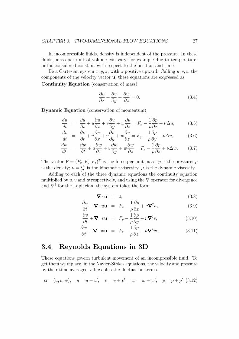
In incompressible fluids, density is independent of the pressure. In thesefluids, mass per unit of volume can vary, for example due to temperature,but is considered constant with respect to the position and time.
Be a Cartesian system x, y, z, with z positive upward. Calling u, v, w thecomponents of the velocity vector u, these equations are expressed as:
Continuity Equation (conservation of mass)
∂u
∂x+∂v
∂y+∂w
∂z= 0. (3.4)
Dynamic Equation (conservation of momentum)
du
dt=
∂u
∂t+ u
∂u
∂x+ v
∂u
∂y+ w
∂u
∂z= Fx −
1
ρ
∂p
∂x+ ν∆u, (3.5)
dv
dt=
∂v
∂t+ u
∂v
∂x+ v
∂v
∂y+ w
∂v
∂z= Fy −
1
ρ
∂p
∂y+ ν∆v, (3.6)
dw
dt=
∂w
∂t+ u
∂w
∂x+ v
∂w
∂y+ w
∂w
∂z= Fz −
1
ρ
∂p
∂z+ ν∆w. (3.7)
The vector F = (Fx, Fy, Fz)T is the force per unit mass; p is the pressure; ρ
is the density; ν =µρ is the kinematic viscosity, µ is the dynamic viscosity.
Adding to each of the three dynamic equations the continuity equationmultiplied by u, v and w respectively, and using the∇ operator for divergenceand ∇2 for the Laplacian, the system takes the form
∇∇∇∇∇∇∇∇∇∇∇∇∇∇ · u = 0, (3.8)
∂u
∂t+∇∇∇∇∇∇∇∇∇∇∇∇∇∇ · uu = Fx −
1
ρ
∂p
∂x+ ν∇∇∇∇∇∇∇∇∇∇∇∇∇∇2u, (3.9)
∂v
∂t+∇∇∇∇∇∇∇∇∇∇∇∇∇∇ · vu = Fy −
1
ρ
∂p
∂y+ ν∇∇∇∇∇∇∇∇∇∇∇∇∇∇2v, (3.10)
∂w
∂t+∇∇∇∇∇∇∇∇∇∇∇∇∇∇ · wu = Fz −
1
ρ
∂p
∂z+ ν∇∇∇∇∇∇∇∇∇∇∇∇∇∇2w. (3.11)
3.4 Reynolds Equations in 3D
These equations govern turbulent movement of an incompressible fluid. Toget them we replace, in the Navier-Stokes equations, the velocity and pressureby their time-averaged values plus the fluctuation terms.
u = (u, v, w), u = u+ u′, v = v + v′, w = w + w′, p = p+ p′ (3.12)
CHAPTER 3. TWO-DIMENSIONAL FLOW EQUATIONS 28
and calculate the time average of each equation, obtaining
∇∇∇∇∇∇∇∇∇∇∇∇∇∇ · u = 0, (3.13)
∂u
∂t+∇∇∇∇∇∇∇∇∇∇∇∇∇∇ · uu +∇∇∇∇∇∇∇∇∇∇∇∇∇∇ · u′u′ = Fx −
1
ρ
∂p
∂x+ ν∇∇∇∇∇∇∇∇∇∇∇∇∇∇2u, (3.14)
∂v
∂t+∇∇∇∇∇∇∇∇∇∇∇∇∇∇ · v u +∇∇∇∇∇∇∇∇∇∇∇∇∇∇ · v′u′ = Fy −
1
ρ
∂p
∂y+ ν∇∇∇∇∇∇∇∇∇∇∇∇∇∇2v, (3.15)
∂w
∂t+∇∇∇∇∇∇∇∇∇∇∇∇∇∇ · w u +∇∇∇∇∇∇∇∇∇∇∇∇∇∇ · w′u′ = Fz −
1
ρ
∂p
∂z+ ν∇∇∇∇∇∇∇∇∇∇∇∇∇∇2w. (3.16)
The resulting equations have the same structure as equations (3.8)-(3.11),with two differences: the variables u, v, w, p have been replaced by theiraverage values and new ones have been added on the left member. If wedevelop them and place them on the right, we obtain the 3D Reynoldsequations:
∇∇∇∇∇∇∇∇∇∇∇∇∇∇ · u = 0, (3.17)
∂u
∂t+∇∇∇∇∇∇∇∇∇∇∇∇∇∇ · uu = Fx −
1
ρ
∂p
∂x+ ν∇∇∇∇∇∇∇∇∇∇∇∇∇∇2u−
[∂u′2
∂x+∂u′v′
∂y+∂u′w′
∂z
], (3.18)
∂v
∂t+∇∇∇∇∇∇∇∇∇∇∇∇∇∇ · v u = Fy −
1
ρ
∂p
∂y+ ν∇∇∇∇∇∇∇∇∇∇∇∇∇∇2v −
[∂u′v′
∂x+∂v′2
∂y+∂v′w′
∂z
], (3.19)
∂w
∂t+∇∇∇∇∇∇∇∇∇∇∇∇∇∇ · w u = Fz −
1
ρ
∂p
∂z+ ν∇∇∇∇∇∇∇∇∇∇∇∇∇∇2w −
[∂u′w′
∂x+∂v′w′
∂y+∂w′2
∂z
].(3.20)
The cross products of the turbulent fluctuations of velocity multiplied bydensity have dimensions of force/area and they are called Reynolds stresses.According to the Boussinesq hypothesis, these stresses are proportional tothe derivative of the time averages of the velocity components, being µt,turbulent dynamic viscosity, the coefficient of proportionality. Operating,simplifying and assuming ν + νt ≈ νt we obtain:
∇∇∇∇∇∇∇∇∇∇∇∇∇∇ · u = 0, (3.21)
∂u
∂t+∇∇∇∇∇∇∇∇∇∇∇∇∇∇ · uu = Fx −
1
ρ
∂p
∂x+∇∇∇∇∇∇∇∇∇∇∇∇∇∇ · νt∇∇∇∇∇∇∇∇∇∇∇∇∇∇u+∇∇∇∇∇∇∇∇∇∇∇∇∇∇ · νt
∂u
∂x, (3.22)
∂v
∂t+∇∇∇∇∇∇∇∇∇∇∇∇∇∇ · v u = Fy −
1
ρ
∂p
∂y+∇∇∇∇∇∇∇∇∇∇∇∇∇∇ · νt∇∇∇∇∇∇∇∇∇∇∇∇∇∇v +∇∇∇∇∇∇∇∇∇∇∇∇∇∇ · νt
∂u
∂y, (3.23)
∂w
∂t+∇∇∇∇∇∇∇∇∇∇∇∇∇∇ · w u = Fz −
1
ρ
∂p
∂z+∇∇∇∇∇∇∇∇∇∇∇∇∇∇ · νt∇∇∇∇∇∇∇∇∇∇∇∇∇∇w +∇∇∇∇∇∇∇∇∇∇∇∇∇∇ · νt
∂u
∂z. (3.24)
These expressions are very similar to the Navier Stokes Eq. (3.8)-(3.11) withthe difference that the instantaneous values of velocity and pressure have

CHAPTER 3. TWO-DIMENSIONAL FLOW EQUATIONS 29
been replaced by their time averages, the viscosity by the turbulent viscosityνt = µt/ρ and a new addend has appeared in the source term, which isnegligible if we assume that the spatial variation of νt is very small.
3.5 The Shallow Water equations
There are flows in nature in which the horizontal dimensions are clearlypredominant. If, in addition, the vertical variation in the horizontal velocitycomponent is small and there are little vertical accelerations, these flowscan often be described by means of a set of equations in two dimensions,resulting of the vertical integration of the 3D equations. To obtain themsome hypothesis are made:
a) Small bottom slope.
b) The distribution of pressure is assumed to be hydrostatic .
c) The main movement of particles occurs in horizontal planes.
d) The vertical distribution of u, v is nearly uniform.
e) The mass forces are gravity and the Coriolis force.
f) The vertical acceleration of the particles is negligible compared to g.
g) The contours friction in unsteady flow, can be evaluated using formulaevalid for steady flow, like Manning.
The shallow water equations in two dimensions are expressed as
∂U
∂t+∂F1
∂x+∂F2
∂y= G, (3.25)
being the variables vector
U =
hhuhv
, (3.26)
terms F1 and F2
F1 =
hu
hu2 + 12gh
2
huv
, F2 =
hvhuv
hv2 + 12gh
2
, (3.27)
CHAPTER 3. TWO-DIMENSIONAL FLOW EQUATIONS 30
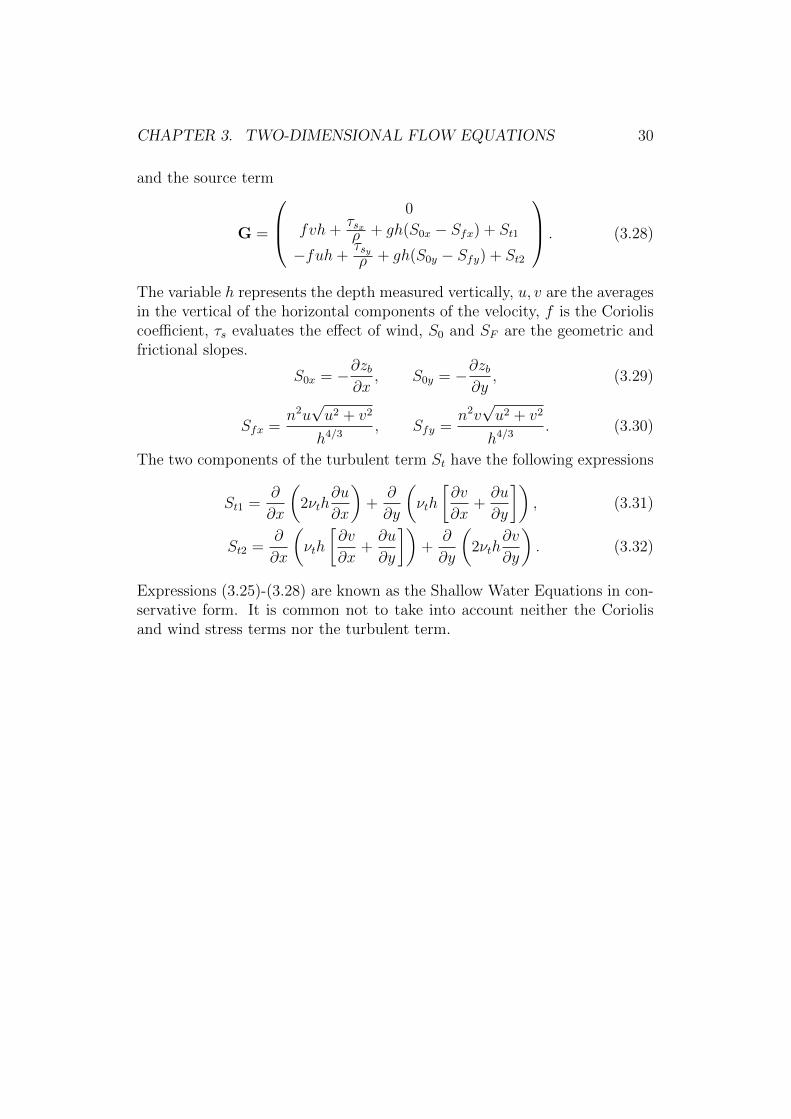
and the source term
G =
0
fvh+τsxρ + gh(S0x − Sfx) + St1
−fuh+τsyρ + gh(S0y − Sfy) + St2
. (3.28)
The variable h represents the depth measured vertically, u, v are the averagesin the vertical of the horizontal components of the velocity, f is the Corioliscoefficient, τs evaluates the effect of wind, S0 and SF are the geometric andfrictional slopes.
S0x = −∂zb∂x
, S0y = −∂zb∂y
, (3.29)
Sfx =n2u√u2 + v2
h4/3, Sfy =
n2v√u2 + v2
h4/3. (3.30)
The two components of the turbulent term St have the following expressions
St1 =∂
∂x
(2νth
∂u
∂x
)+
∂
∂y
(νth
[∂v
∂x+∂u
∂y
]), (3.31)
St2 =∂
∂x
(νth
[∂v
∂x+∂u
∂y
])+
∂
∂y
(2νth
∂v
∂y
). (3.32)
Expressions (3.25)-(3.28) are known as the Shallow Water Equations in con-servative form. It is common not to take into account neither the Coriolisand wind stress terms nor the turbulent term.
Chapter 4
Application to the 2D SWE
4.1 Types of finite volumes
The use of the finite volume method in computational fluid dynamics isrelatively recent. According to Hirsch [17, pg. 237] it was introduced byMcDonald in 1971 and independently by Mc Cormack and Paullay in 1972for solving the Euler equations in 2D. In 1973 Rizzi and Inouye extended itto three-dimensional flows. Eymard et al. [13] attribute their introduction,ten years earlier, to Tichonov and Samarskii for solving convection-diffusionequations. In [13, pg. 9] a long list of works devoted to the mathematicalanalysis of the method is mentioned.
To use this method we usually start from a previous discretization of thecomputational domain in elements, normally triangles or quadrangles, fromwhich the new mesh or finite volume cells is built. In each of these volumesthe integral form of the equations is obtained, simplified by applying thedivergence theorem and discretized. The resulting expressions establish theexact conservation of relevant flow properties in each cell. The terms ofthe equations are replaced by approximations of the finite difference type,obtaining algebraic equations that are solved by an iterative process. Webriefly describe below some of the most commonly used finite volumes [4, 15].
4.1.1 Cell-type finite volumes
The cell type (or cell-center) finite volumes [15, pg. 366] are the same initialgrid cells and the values of the dependent variables are stored in the cellcenter (centers of quadrilaterals or barycenters of triangles). This methodhas the advantage of using the initial mesh and the disadvantage that thenodes to which the variables values are assigned -which represent the cell
31
CHAPTER 4. APPLICATION TO THE 2D SWE 32
values and are used in the discretization- do not coincide with the nodes ofthe original mesh.
4.1.2 Vertex-type finite volumes
The vertex type (or cell-vertex) finite volumes [15, pg. 368] use the vertices ofthe initial mesh as nodes of the finite volume mesh and the new cells are builtaround them. In contrast to the previous case, the initial mesh vertices areused and assigned the variables values in each finite volume. In this methodthe implementation of boundary conditions is simpler, since the value of thevariables in the boundary nodes are known. The drawback is that a newmesh has to be built (dual mesh).
4.1.3 Edge-type finite volumes
This type of finite volumes, not usual in literature, is described in [31, pg.87]. To obtain them we start from a mesh formed by triangles, each of whichis divided into three, by joining each vertex with the barycentre. Then thesubtriangles are joined in pairs so that each finite volume is formed by thetwo subtriangles with an edge of the initial mesh in common. The centerof the finite volume is the midpoint of the edge. With this method, theangular points of the contour -that belong to the initial mesh- are not nodesof the finite volume mesh, what avoids two difficulties. The first is relatedto the velocity vector: since fluid do not passes through the walls, in nodescorresponding to solid boundary the velocity vector must be parallel to theboundary, which gives problems in angular points. Another difficulty is thecalculation of the perpendicular to the boundary edges at such points, whichhave two perpendicular. On the other hand, the initial nodes are not used.To obtain the values in these nodes we must interpolate.
4.2 Description of the finite volumes used
The finite volumes used in this work are based on a triangular discretizationof the domains so that the nodes of the triangular mesh are used as the nodesof the finite volume mesh.
For each node I, the barycenters of the triangles with I as a common vertexand the mid-points of the edges that meet at I are taken. The boundary Γi
of the cell Ci is obtained by joining these points and Γij = AMB representsthe common part of Γi and Γj.

CHAPTER 4. APPLICATION TO THE 2D SWE 33
The outward normal vector to Γij is ηηηηηηηηηηηηηηij and it can be different at AM
and at MB. The norm of ηηηηηηηηηηηηηηij, ‖ηηηηηηηηηηηηηηij‖, is the length of the edge and ηηηηηηηηηηηηηηij is thecorresponding unit vector
ηηηηηηηηηηηηηηij =ηηηηηηηηηηηηηηij‖ηηηηηηηηηηηηηηij‖
= (αij, βij)T . (4.1)
The subcell Tij is the union of triangles AMI and MBI (see Figure 4.1). Theirareas are
Aij1 =‖ηAM
ij ‖dAMij
2, Aij2 =
‖ηMBij ‖dMB
ij
2, (4.2)
where the values dij represent the triangle height.
Ti j
A
M
B
BAM
�ij
I
J
J
I
K
�i
Ci
�ij
AM
�ij
MB
Figure 4.1: Construction of the finite volumes.
4.3 Terms considered in the equations
To apply the finite volume method to the Shallow Water Equations, first onehas to decide which parts of the source term will be taken into account. Inthis regard, 1) the Coriolis term has almost no importance if the domain isnot large; 2) it is usually neglected the influence of the wind, although in somecases, such as estuaries of some magnitude, it may be advisable to consider
CHAPTER 4. APPLICATION TO THE 2D SWE 34
it; and 3) the turbulent term is frequently not taken into consideration,assuming that its effects are included in the bottom friction term.
Removing the mentioned addends from the source term the equations(3.25)-(3.28) reduce to
∂U
∂t+∂F1
∂x+∂F2
∂y= G, (4.3)
being
U =
hhuhv
, F1 =
hu
hu2 + 12gh
2
huv
, F2 =
hvhuv
hv2 + 12gh
2
, (4.4)
G =
0gh(S0x − Sfx)gh(S0y − Sfy)
. (4.5)
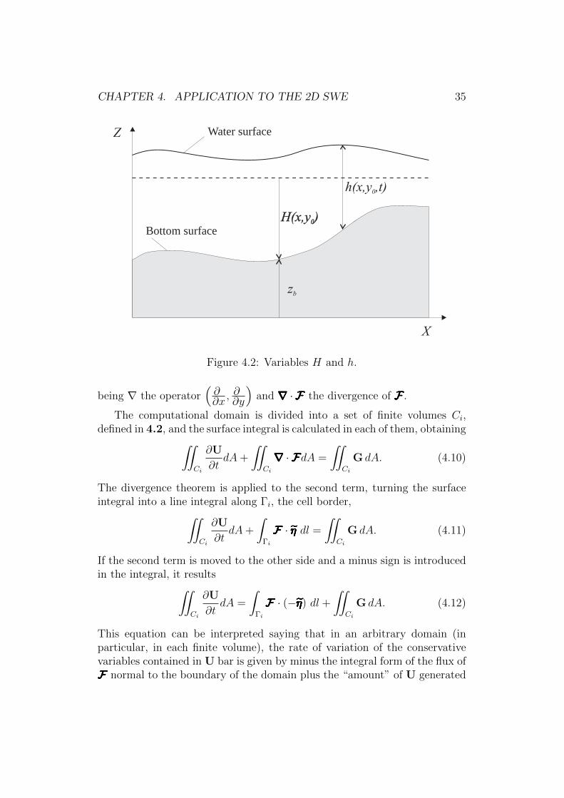
The geometric slopes, defined in terms of zb by (3.29) (see Fig.4.2), will beexpressed in terms of H, which represents the distance to the bottom from afixed reference level, positive downward. Thus the slopes are positive if theground descend and negative otherwise.
S0x =∂H
∂x, S0y =
∂H
∂y. (4.6)
The friction slopes are
Sfx =n2u√u2 + v2
h4/3, Sfy =
n2v√u2 + v2
h4/3, (4.7)
where n is the Manning coefficient, h the depth and u, v the horizontal com-ponents of the velocity. The conservative variables hu, hv represent the dis-charge per unit width in a rectangular channel. In Figure 4.2 a section ofthe domain by a vertical plane y = y0 is represented.
4.4 Integration and discretization
Using the simbolic notation
FFFFFFFFFFFFFF(U) = (F1(U),F2(U)), (4.8)
the system (4.3) can be written in a more compact form
∂U
∂t+∇∇∇∇∇∇∇∇∇∇∇∇∇∇ · FFFFFFFFFFFFFF = G, (4.9)
CHAPTER 4. APPLICATION TO THE 2D SWE 35
Z
X
h(x,y ,t)0
H(x,y )0H(x,y )0
Water surface
Bottom surface
zb
Figure 4.2: Variables H and h.
being ∇ the operator(∂∂x, ∂∂y
)and ∇∇∇∇∇∇∇∇∇∇∇∇∇∇ · FFFFFFFFFFFFFF the divergence of FFFFFFFFFFFFFF .
The computational domain is divided into a set of finite volumes Ci,defined in 4.2, and the surface integral is calculated in each of them, obtaining∫∫
Ci
∂U
∂tdA+
∫∫Ci
∇∇∇∇∇∇∇∇∇∇∇∇∇∇ · FFFFFFFFFFFFFFdA =
∫∫Ci
G dA. (4.10)
The divergence theorem is applied to the second term, turning the surfaceintegral into a line integral along Γi, the cell border,∫∫
Ci
∂U
∂tdA+
∫Γi
FFFFFFFFFFFFFF · ηηηηηηηηηηηηηη dl =
∫∫Ci
G dA. (4.11)
If the second term is moved to the other side and a minus sign is introducedin the integral, it results∫∫
Ci
∂U
∂tdA =
∫Γi
FFFFFFFFFFFFFF · (−ηηηηηηηηηηηηηη) dl +
∫∫Ci
G dA. (4.12)
This equation can be interpreted saying that in an arbitrary domain (inparticular, in each finite volume), the rate of variation of the conservativevariables contained in U bar is given by minus the integral form of the flux ofFFFFFFFFFFFFFF normal to the boundary of the domain plus the “amount” of U generated
CHAPTER 4. APPLICATION TO THE 2D SWE 36
in the domain [22, pg. 6.20]. That is, the variation in time of U is due tothe net flux of FFFFFFFFFFFFFF towards the inside of the cell plus the variation due to thesource term.
4.4.1 Discretization of the time derivative
The solution of equation (4.3) is approximated by some values Uni , constant
in each cell Ci and time tn, which are assigned to node I corresponding tothe cell.
The time derivative is discretized by the Forward Euler Method
∂U
∂t
∣∣∣∣Ci,tn
≈ Un+1i −Un
i
4t. (4.13)
Then equation (4.11) becomes∫∫Ci
Un+1i −Un
i
4tdA+
∫Γi
FFFFFFFFFFFFFF · ηηηηηηηηηηηηηη dl =
∫∫Ci
GdA. (4.14)
In the first term, Un+1i , Un
i and 4t have constant values in the cell, so theycan go out of the integral, resulting∫∫
Ci
Un+1i −Un
i
4tdA =
Un+1i −Un
i
4tAi. (4.15)
4.4.2 Integration of the flux and source terms
In the second addend of (4.14) the line integral splits in a sum of integralsalong each of the edges Γij, j ∈ Ki∫
Γi
FFFFFFFFFFFFFF · ηηηηηηηηηηηηηη dl =∑j∈Ki
∫Γij
FFFFFFFFFFFFFF · ηηηηηηηηηηηηηη dl. (4.16)
The surface integral of the source term splits into a sum of integrals over thesubcells Tij, j ∈ Ki ∫∫
Ci
GdA =∑j∈Ki
∫∫Tij
GdA. (4.17)
Thus (4.14) becomes
Un+1i −Un
i
4tAi +
∑j∈Ki
∫Γij
FFFFFFFFFFFFFF · ηηηηηηηηηηηηηη dl =∑j∈Ki
∫∫Tij
GdA. (4.18)

CHAPTER 4. APPLICATION TO THE 2D SWE 37
4.4.3 Definition of the discretized flux
The sum (4.16) will now be expressed in terms of the values of the variablesat node I and Nj, j ∈ Ki, using an upwind scheme.
The dot product of FFFFFFFFFFFFFF and ηηηηηηηηηηηηηη is called 2D flux through a segment of unitlength
Z = FFFFFFFFFFFFFF · ηηηηηηηηηηηηηη = αF1 + βF2, (4.19)
where (α, β) are the components of the unit vector normal to the edge.To discretize the flux different proposals have been made. In this case,
we will use the Van Leer Q-scheme [30], as proposed in [5, 31].The Q-schemes are a family of upwind schemes, in which the numerical
flow is obtained as follows
φφφφφφφφφφφφφφ(Uni ,U
nj , ηηηηηηηηηηηηηηij) =
Z(Uni , ηηηηηηηηηηηηηηij) + Z(Un
j , ηηηηηηηηηηηηηηij)
2− 1
2
∣∣Q(UnQ, ηηηηηηηηηηηηηηij)
∣∣ (Unj −Un
i ),
(4.20)where Un
i , Unj represent the values of the variables vector at I and J ; Q is
the jacobian matrix of flux
Q =dZ
dU= α
dF1
dU+ β
dF2
dU; (4.21)
Matrix |Q| is obtained as
|Q| = X |Λ|X−1, (4.22)
being |Λ| the diagonal matrix of the absolute values of the eigenvectors of Qand X the matrix whose columns are the eigenvectors of Q; in the Van LeerQ-scheme, |Q| is evaluated in the intermediate state
UnQ =
Uni + Un
j
2. (4.23)
Then, expression (4.20) that discretizes the 2D flux in the middle point be-tween I and J is obtained as the mean value of the fluxes at both points plusan upwinding term.
Note that in (4.21), the derivatives of F1 and F2 with respect to thevariables vector U are the factors that appear when writing the equation(4.3) in the nonconservative form.
∂U
∂t+∂F1
∂x+∂F2
∂y=∂U
∂t+
dF1
dU
∂U
∂x+
dF2
dU
∂U
∂y= G. (4.24)

CHAPTER 4. APPLICATION TO THE 2D SWE 38
The shallow water equations are a strictly hyperbolic system (see 2.7), i.e.the flux Jacobian matrix has three different eigenvalues and three linearlyindependent eigenvectors, so there will always be X−1. Indeed
dF1
dU=
0 1 0−u2 + gh 2u 0−uv v u
, (4.25)
dF2
dU=
0 0 1−uv v u
−v2 + gh 0 2v
, (4.26)
therefore, applying (4.21), it results
dZ
dU=
0 α β
α(−u2 + gh) + β(−uv) 2αu+ βv βu
α(−uv) + β(−v2 + gh) αv αu+ 2βv
. (4.27)
If c is the speed of the wavec =
√gh, (4.28)
the eigenvalues of the Jacobian matrix are
λ1 = αu+ βv,
λ2 = λ1 + c, (4.29)
λ3 = λ1 − c,
and matrices |Λ| , X and X−1 can be calculated
|Λ| =
|λ1| 0 00 |λ2| 00 0 |λ3|
, (4.30)
X =
0 1 1
−βc u+ αc u− αcαc v + βc v − βc
, (4.31)
X−1 =1
2c
2βu− 2αv −2β 2α
c− αu− βv α β
c+ αu+ βv −α −β
. (4.32)
CHAPTER 4. APPLICATION TO THE 2D SWE 39
Thus, the second member of (4.16) is discretized as∑j∈Ki
∫Γij
FFFFFFFFFFFFFF · ηηηηηηηηηηηηηη dl ≈∑j∈Ki
‖ηηηηηηηηηηηηηηij‖φφφφφφφφφφφφφφnij, (4.33)
being φφφφφφφφφφφφφφnij the discretized unit flux
φφφφφφφφφφφφφφnij =
(αF1 + βF2)ni + (αF1 + βF2)nj2
− 1
2(X |Λ|X−1)Un
Q(Un
j −Uni ). (4.34)
4.4.4 Definition of the discretized source
The convenience of the upwinding of the source term has been analyzedby Vazquez Cendon [31]. In this work she studies the discretization of thegeometric source term in the 1D shallow water equations and proposes, forthe 2D case, an extension of the 1D expression, verifying that gives goodresults. Here we will upwind the source term containing the geometric slopeand calculate the friction slope in the center of each cell. According to theabove, the two-dimensional discretized source in each subcell Tij is definedas
ψψψψψψψψψψψψψψ = X(I− |Λ|Λ−1)X−1G0 + Gf , (4.35)
ψψψψψψψψψψψψψψ = (I− |Q|Q−1)G0 + Gf where X,X−1, |Λ| and Λ−1 are calculated at(Un
Q, ηηηηηηηηηηηηηηij), Matrices |Λ| , X y X−1 are given respectively by (4.30), (4.31) and(4.32). Λ−1 is
Λ−1 =
1/λ1 0 00 1/λ2 00 0 1/λ3
, (4.36)
G0 approximates the geometric source term
G0 =
0
ghni + hnj
2Hj −Hi
dijα
ghni + hnj
2Hj −Hi
dijβ
(4.37)
and Gf approximates the friction source term, evaluated en each cell center.
Gf =
0
ghni (−Sfx)ni
ghni (−Sfy)ni
. (4.38)
CHAPTER 4. APPLICATION TO THE 2D SWE 40
(α, β) and dij take the values given by expressions (4.1) and (4.2) and thefriction slopes aregiven by (4.7). The sum of (4.17) is then expressed as∑
j∈Ki
∫∫Tij
G dA ≈∑j∈Ki
Aijψψψψψψψψψψψψψψnij, (4.39)
where Aij takes the expressions given in (4.2) for each subtriangle of thesubcell Tij and ψψψψψψψψψψψψψψn
ij is calculated from (4.35). Note that dij represents thedistance from I to the edge AM .
4.4.5 Discretization of the boundary conditions
To discretize the flux term in the contour of the cell and the source termin each subcell we use the variables values at I and its neighbor J . In thecase of the boundary nodes, there are no neighboring nodes on the other sideof the edge (Figure 4.1). We assume, for these edges, that the neighboringnode is the same node I, which means that we do not upwind the flux (asthe upwinding term is zero). Furthermore, the area of each subcell is a factorof the discretized source. As edges have zero area, we do not consider thesource terms in these nodes.
4.4.6 Obtaining of the time step
There are different expressions for calculating the time step that ensuresstability. For the one dimensional case, taking a maximum value of Courantnumber equal to 1, the condition used in [18, pg. 283] is
4t ≤ min (4x)imax (|u|+ c)i
, (4.40)
being (4x)i the cell width, u the velocity and c the celerity.For the 2D case, [1, pg. 233] proposes
4t ≤ min
(Dij
2(√u2 + v2 + c)ij
), (4.41)
being Dij the distances beween node I and its four neighborgs. This hasbeen the formula used in the present work.
CHAPTER 4. APPLICATION TO THE 2D SWE 41
4.5 Algorithm
A forward discretization of the time derivative and two others for the fluxand source terms, which are evaluated at time tn have been obtained. Thus(4.18) now takes the form
Un+1i −Un
i
4tAi +
∑j∈Ki
‖ηηηηηηηηηηηηηηij‖φφφφφφφφφφφφφφnij =
∑j∈Ki
Aijψψψψψψψψψψψψψψnij, (4.42)
from where
Un+1i = Un
i +4tAi
(∑j∈Ki
Aijψψψψψψψψψψψψψψnij −
∑j∈Ki
‖ηηηηηηηηηηηηηηij‖φφφφφφφφφφφφφφnij
). (4.43)
The above expression provides a explicit in time iterative method for cal-culating the value of the variables vector U on each node I and in everymoment, from the variables values in the previous time, on the same node Iand the Nj, j ∈ Ki that surround it.

Chapter 5
Some results
5.1 Types of boundary conditions
The conditions usually used for channel flow are of Dirichlet type: the valuesof some variables at certain points are set.
• Upstream section. In subcritical flow: discharge. In supercritical flow:discharge and depth.
• Downstream section. In subcritical flow: depth. In supercritical flow:none.
• Side walls: In channels where we simulate unidimensional flow, weimpose the slip-condition, i.e. we cancel the velocity component per-pendicular to the wall. This means considering section wide enough toneglect the friction on the walls. In the two-dimensional flow, the wallfriction is considered by changing the value of the hydraulic radius ofthe nodes in contact with it.
5.2 One dimensional problems
Both the one dimensional and the two dimensional examples have been cal-culated with the two dimensional model. In the one dimensional ones asymmetric channel with a symmetric mesh has been considered with the slip-condition (no friction) as the boundary condition in walls. In these cases, werepresent the depth along a longitudinal section.
42
CHAPTER 5. SOME RESULTS 43
5.2.1 Straight channel with slope and bottom friction
The calculations have been performed for a channel 2 m wide by 1, 000 mlong. The mesh is formed by right angled triangles whose arms are 1 m longwith a total of 3003 nodes. The unit discharge is q = 4 m2/s, and the criticaldepth is
yc =
(q2
g
)1/3
= 1.18 m. (5.1)
Two flows, one subcritical and another supercritical have been simulated.
a) Subcritical flow: The slope is S0 = 0.001 and the Manning coefficientn = 0.015 (concrete) [10, pg. 109]. The normal depth is
yn =n0.6q0.6
S 0.30
= 1.47 m, (5.2)
greater than yc. As the flow is subcritical, the imposed boundary con-ditions are: discharge at the inlet section and depth at the outlet. Twocases are solved: the first one with an imposed depth of hbc = 1.75 m,greater than yn, the second one with hbc = 1.20 m < yn. In both casesthe initial conditions are still water and constant depth equal to thehbc. The flow profile (of type M1 and M2, respectively) can be seen infigures 5.1 and 5.2. In both cases the depth gradually approaches itsnormal value.
b) Supercritical flow: The values are S0 = 0.002 and n = 0.01 (glass). Inthis case the normal depth results
yn =n0.6q0.6
S 0.30
= 0.94 m, (5.3)
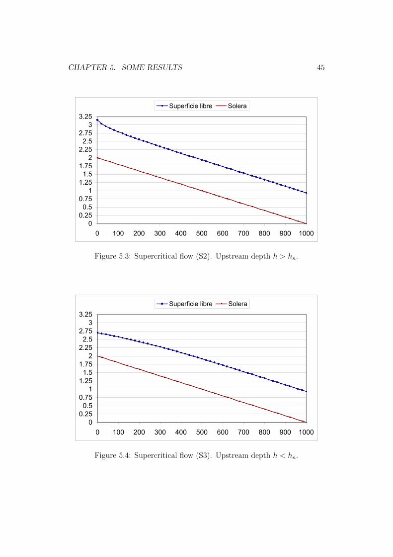
smaller than yc. The boundary conditions (supercritical flow) are im-posed at the inlet. In the first case hbc = 1.15 m > yn and in the secondhbc = 0.70 m < yn. The initial conditions are the same as above. Theflow profiles are of types S2 and S3, (figures 5.3 and 5.4 respectively).Again the depth gradually approaches its normal value in both cases.
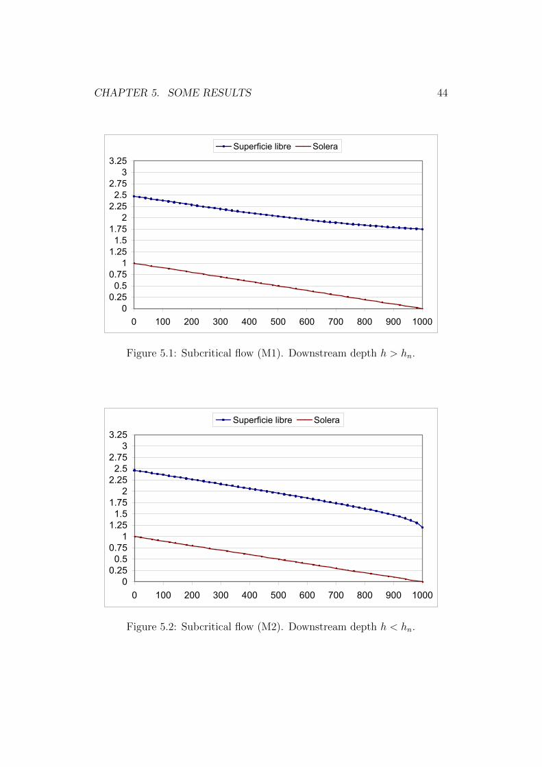
CHAPTER 5. SOME RESULTS 44
Y H Z0 H+Z00 1.472732 1 2.472732 2
20 1.474945 0.98 2.454945 240 1.47571 0.96 2.43571 260 1.476548 0.94 2.416548 280 1.477465 0.92 2.397465 2
100 1.478467 0.9 2.378467 2120 1.479562 0.88 2.359562 2140 1.480755 0.86 2.340755 2160 1.482057 0.84 2.322057 2180 1.483476 0.82 2.303476 2200 1.485022 0.8 2.285022 2220 1.486704 0.78 2.266704 2240 1.488532 0.76 2.248532 2260 1.490514 0.74 2.230514 2280 1.492658 0.72 2.212658 2300 1.494974 0.7 2.194974 2320 1.497472 0.68 2.177472 2340 1.500161 0.66 2.160161 2360 1.503053 0.64 2.143053 2380 1.506158 0.62 2.126158 2400 1.509489 0.6 2.109489 2420 1.513055 0.58 2.093055 2440 1.516869 0.56 2.076869 2460 1.520941 0.54 2.060941 2480 1.525283 0.52 2.045283 2500 1.529904 0.5 2.029904 2520 1.534814 0.48 2.014814 2540 1.540022 0.46 2.000022 2560 1.545537 0.44 1.985537 2580 1.551366 0.42 1.971366 2600 1.557516 0.4 1.957516 2620 1.563993 0.38 1.943993 2640 1.570802 0.36 1.930802 2660 1.577945 0.34 1.917945 2680 1.585425 0.32 1.905425 2700 1.593244 0.3 1.893244 2720 1.601401 0.28 1.881401 2740 1.609898 0.26 1.869898 2760 1.618732 0.24 1.858732 2780 1.627903 0.22 1.847903 2800 1.637408 0.2 1.837408 2820 1.647245 0.18 1.827245 2840 1.657409 0.16 1.817409 2860 1.667896 0.14 1.807896 2880 1.6787 0.12 1.7987 2900 1.689816 0.1 1.789816 2920 1.701237 0.08 1.781237 2940 1.712955 0.06 1.772955 2960 1.724964 0.04 1.764964 2980 1.737255 0.02 1.757255 2
1000 1.75 0 1.75 2
00.250.5
0.751
1.251.5
1.752
2.252.5
2.753
3.25
0 100 200 300 400 500 600 700 800 900 1000
Superficie libre Solera
Figure 5.1: Subcritical flow (M1). Downstream depth h > hn.
Y H Z0 H+Z00 1.466015 1 2.466015 2
20 1.467507 0.98 2.447507 240 1.467411 0.96 2.427411 260 1.467304 0.94 2.407304 280 1.467185 0.92 2.387185 2
100 1.467052 0.9 2.367052 2120 1.466906 0.88 2.346906 2140 1.466743 0.86 2.326743 2160 1.466563 0.84 2.306563 2180 1.466363 0.82 2.286363 2200 1.466143 0.8 2.266143 2220 1.465899 0.78 2.245899 2240 1.46563 0.76 2.22563 2260 1.465333 0.74 2.205333 2280 1.465004 0.72 2.185004 2300 1.464642 0.7 2.164642 2320 1.464242 0.68 2.144242 2340 1.4638 0.66 2.1238 2360 1.463313 0.64 2.103313 2380 1.462775 0.62 2.082775 2400 1.46218 0.6 2.06218 2420 1.461524 0.58 2.041524 2440 1.460799 0.56 2.020799 2460 1.459998 0.54 1.999998 2480 1.459113 0.52 1.979113 2500 1.458133 0.5 1.958133 2520 1.457049 0.48 1.937049 2540 1.455848 0.46 1.915848 2560 1.454516 0.44 1.894516 2580 1.453038 0.42 1.873038 2600 1.451396 0.4 1.851396 2620 1.449569 0.38 1.829569 2640 1.447535 0.36 1.807535 2660 1.445264 0.34 1.785264 2680 1.442726 0.32 1.762726 2700 1.439882 0.3 1.739882 2720 1.436688 0.28 1.716688 2740 1.433088 0.26 1.693088 2760 1.429019 0.24 1.669019 2780 1.424398 0.22 1.644398 2800 1.419126 0.2 1.619126 2820 1.413075 0.18 1.593075 2840 1.406077 0.16 1.566077 2860 1.397908 0.14 1.537908 2880 1.388256 0.12 1.508256 2900 1.376669 0.1 1.476669 2920 1.36244 0.08 1.44244 2940 1.344365 0.06 1.404365 2960 1.320071 0.04 1.360071 2980 1.283401 0.02 1.303401 2
1000 1.2 0 1.2 2
00.25
0.50.75
11.25
1.51.75
22.25
2.52.75
33.25
0 100 200 300 400 500 600 700 800 900 1000
Superficie libre Solera
Figure 5.2: Subcritical flow (M2). Downstream depth h < hn.
CHAPTER 5. SOME RESULTS 45
Y H Z0 H+Z00 1.15 2 3.15 2
20 1.076159 1.96 3.036159 240 1.041311 1.92 2.961311 260 1.019393 1.88 2.899393 280 1.003739 1.84 2.843739 2
100 0.991874 1.8 2.791874 2120 0.982563 1.76 2.742563 2140 0.975088 1.72 2.695088 2160 0.968991 1.68 2.648991 2180 0.963958 1.64 2.603958 2200 0.959768 1.6 2.559768 2220 0.956253 1.56 2.516253 2240 0.95329 1.52 2.47329 2260 0.95078 1.48 2.43078 2280 0.948646 1.44 2.388646 2300 0.946827 1.4 2.346827 2320 0.945272 1.36 2.305272 2340 0.94394 1.32 2.26394 2360 0.942797 1.28 2.222797 2380 0.941815 1.24 2.181815 2400 0.94097 1.2 2.14097 2420 0.940243 1.16 2.100243 2440 0.939615 1.12 2.059615 2460 0.939074 1.08 2.019074 2480 0.938607 1.04 1.978607 2500 0.938203 1 1.938203 2520 0.937854 0.96 1.897854 2540 0.937553 0.92 1.857553 2560 0.937292 0.88 1.817292 2580 0.937066 0.84 1.777066 2600 0.936871 0.8 1.736871 2620 0.936702 0.76 1.696702 2640 0.936556 0.72 1.656556 2660 0.936431 0.68 1.616431 2680 0.936328 0.64 1.576328 2700 0.936252 0.6 1.536252 2720 0.936207 0.56 1.496207 2740 0.936196 0.52 1.456196 2760 0.936206 0.48 1.416206 2780 0.936226 0.44 1.376226 2800 0.93625 0.4 1.33625 2820 0.936274 0.36 1.296274 2840 0.9363 0.32 1.2563 2860 0.936326 0.28 1.216326 2880 0.936353 0.24 1.176353 2900 0.936381 0.2 1.136381 2920 0.936409 0.16 1.096409 2940 0.936439 0.12 1.056439 2960 0.93647 0.08 1.01647 2980 0.936501 0.04 0.976501 2
1000 0.936773 0 0.936773 2
00.25
0.50.75
11.25
1.51.75
22.25
2.52.75
33.25
0 100 200 300 400 500 600 700 800 900 1000
Superficie libre Solera
Figure 5.3: Supercritical flow (S2). Upstream depth h > hn.
Y H Z0 H+Z00 0.7 2 2.7 2
20 0.717175 1.96 2.677175 240 0.733436 1.92 2.653436 260 0.748993 1.88 2.628993 280 0.763832 1.84 2.603832 2
100 0.777942 1.8 2.577942 2120 0.791314 1.76 2.551314 2140 0.803942 1.72 2.523942 2160 0.815822 1.68 2.495822 2180 0.826956 1.64 2.466956 2200 0.837347 1.6 2.437347 2220 0.847007 1.56 2.407007 2240 0.855947 1.52 2.375947 2260 0.864188 1.48 2.344188 2280 0.871751 1.44 2.311751 2300 0.878662 1.4 2.278662 2320 0.884953 1.36 2.244953 2340 0.890655 1.32 2.210655 2360 0.895803 1.28 2.175803 2380 0.900434 1.24 2.140434 2400 0.904585 1.2 2.104585 2420 0.908294 1.16 2.068294 2440 0.911597 1.12 2.031597 2460 0.914531 1.08 1.994531 2480 0.917129 1.04 1.957129 2500 0.919425 1 1.919425 2520 0.921449 0.96 1.881449 2540 0.92323 0.92 1.84323 2560 0.924794 0.88 1.804794 2580 0.926166 0.84 1.766166 2600 0.927367 0.8 1.727367 2620 0.928418 0.76 1.688418 2640 0.929335 0.72 1.649335 2660 0.930136 0.68 1.610136 2680 0.930834 0.64 1.570834 2700 0.931442 0.6 1.531442 2720 0.931972 0.56 1.491972 2740 0.932433 0.52 1.452433 2760 0.932833 0.48 1.412833 2780 0.933182 0.44 1.373182 2800 0.933484 0.4 1.333484 2820 0.933747 0.36 1.293747 2840 0.933973 0.32 1.253973 2860 0.934157 0.28 1.214157 2880 0.934279 0.24 1.174279 2900 0.934329 0.2 1.134329 2920 0.934328 0.16 1.094328 2940 0.934303 0.12 1.054303 2960 0.934271 0.08 1.014271 2980 0.934237 0.04 0.974237 2
1000 0.932569 0 0.932569 2
00.25
0.50.75
11.25
1.51.75
22.25
2.52.75
33.25
0 100 200 300 400 500 600 700 800 900 1000
Superficie libre Solera
Figure 5.4: Supercritical flow (S3). Upstream depth h < hn.
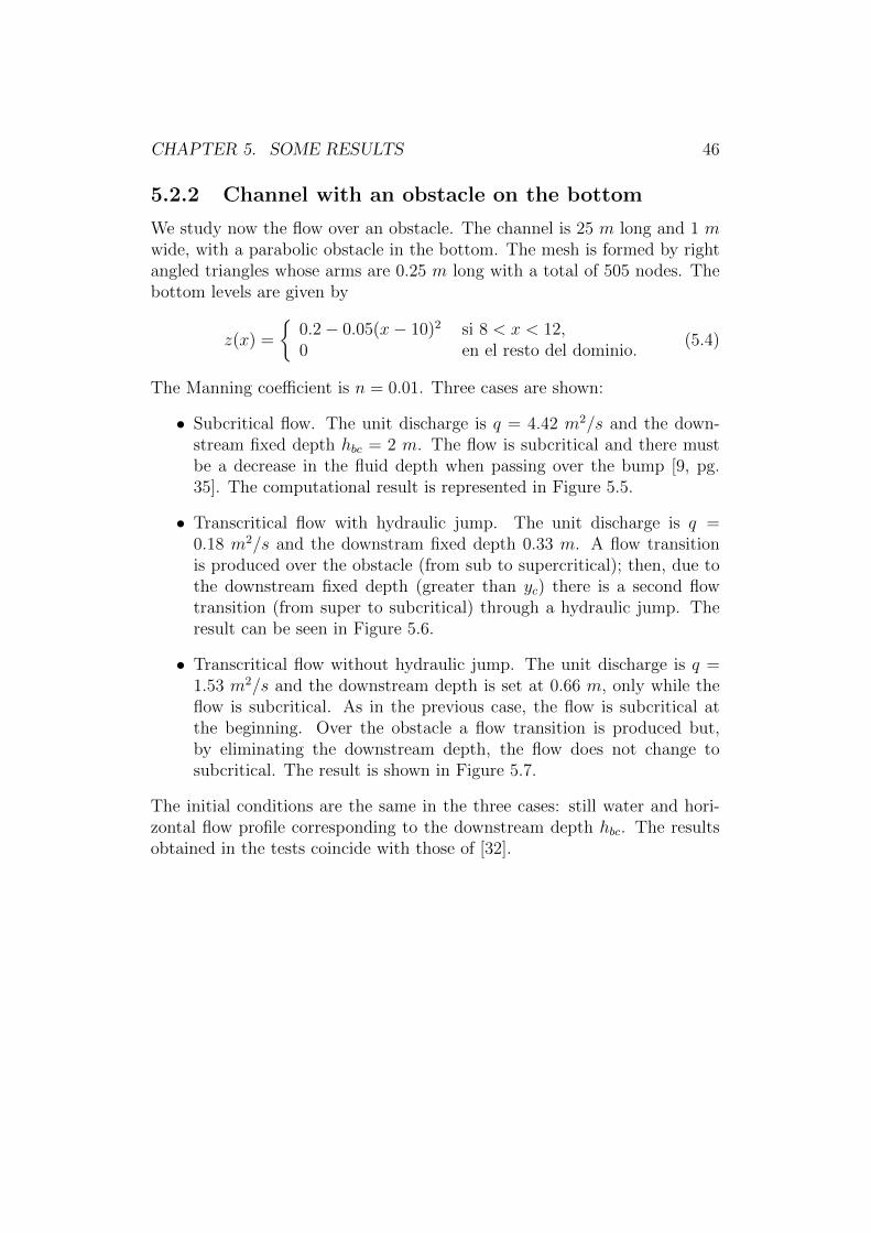
CHAPTER 5. SOME RESULTS 46
5.2.2 Channel with an obstacle on the bottom
We study now the flow over an obstacle. The channel is 25 m long and 1 mwide, with a parabolic obstacle in the bottom. The mesh is formed by rightangled triangles whose arms are 0.25 m long with a total of 505 nodes. Thebottom levels are given by
z(x) =
{0.2− 0.05(x− 10)2 si 8 < x < 12,0 en el resto del dominio.
(5.4)
The Manning coefficient is n = 0.01. Three cases are shown:
• Subcritical flow. The unit discharge is q = 4.42 m2/s and the down-stream fixed depth hbc = 2 m. The flow is subcritical and there mustbe a decrease in the fluid depth when passing over the bump [9, pg.35]. The computational result is represented in Figure 5.5.
• Transcritical flow with hydraulic jump. The unit discharge is q =0.18 m2/s and the downstram fixed depth 0.33 m. A flow transitionis produced over the obstacle (from sub to supercritical); then, due tothe downstream fixed depth (greater than yc) there is a second flowtransition (from super to subcritical) through a hydraulic jump. Theresult can be seen in Figure 5.6.
• Transcritical flow without hydraulic jump. The unit discharge is q =1.53 m2/s and the downstream depth is set at 0.66 m, only while theflow is subcritical. As in the previous case, the flow is subcritical atthe beginning. Over the obstacle a flow transition is produced but,by eliminating the downstream depth, the flow does not change tosubcritical. The result is shown in Figure 5.7.
The initial conditions are the same in the three cases: still water and hori-zontal flow profile corresponding to the downstream depth hbc. The resultsobtained in the tests coincide with those of [32].
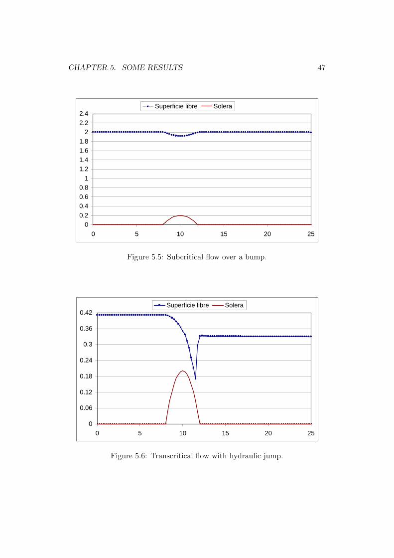
CHAPTER 5. SOME RESULTS 47
00.20.40.60.8
11.21.41.61.8
22.22.4
0 5 10 15 20 25
Superficie libre Solera
Figure 5.5: Subcritical flow over a bump.
0.54290.5430.5430.54310.54310.54320.54330.54330.54340.54340.54350.54360.54360.54370.54370.54380.54390.54390.5440.5440.54410.54420.54420.54430.54430.54440.54450.54450.54460.54460.54470.54480.54480.54490.54490.5450.5450.54510.54520.54520.54530.54530.54540.54550.54550.5456
0
0.06
0.12
0.18
0.24
0.3
0.36
0.42
0 5 10 15 20 25
Superficie libre Solera
Figure 5.6: Transcritical flow with hydraulic jump.
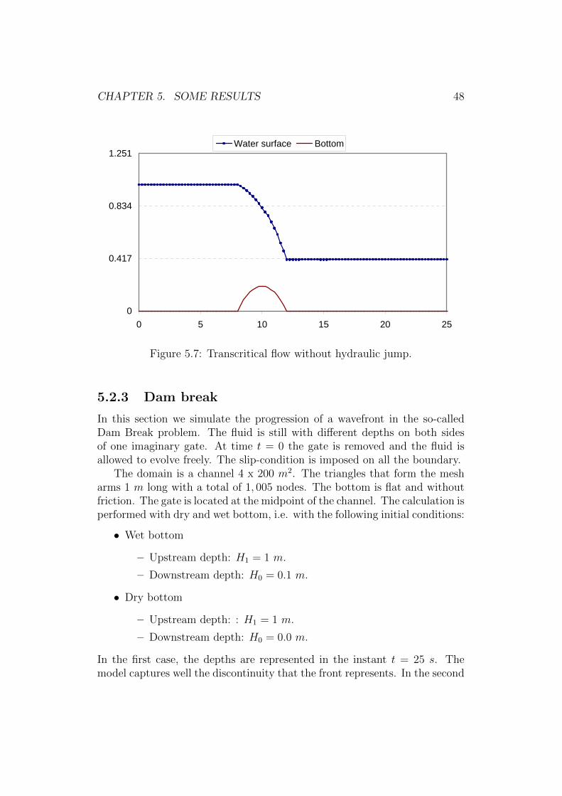
CHAPTER 5. SOME RESULTS 48
1.52351.52351.52351.52351.52351.52351.52351.52351.52351.52351.52351.52331.52261.51951.5991.69841.80541.91862.03762.16212.29162.42542.5582.65362.82222.98583.13733.35133.53973.72483.72513.72543.72553.72553.72553.72553.72543.72543.72553.7256
0
0.14
0.28
0.42
0 5 10 15 20 25
Water surface Bottom
0
0.417
0.834
1.251
0 5 10 15 20 25
Water surface Bottom
Figure 5.7: Transcritical flow without hydraulic jump.
5.2.3 Dam break
In this section we simulate the progression of a wavefront in the so-calledDam Break problem. The fluid is still with different depths on both sidesof one imaginary gate. At time t = 0 the gate is removed and the fluid isallowed to evolve freely. The slip-condition is imposed on all the boundary.
The domain is a channel 4 x 200 m2. The triangles that form the mesharms 1 m long with a total of 1, 005 nodes. The bottom is flat and withoutfriction. The gate is located at the midpoint of the channel. The calculation isperformed with dry and wet bottom, i.e. with the following initial conditions:
• Wet bottom
– Upstream depth: H1 = 1 m.
– Downstream depth: H0 = 0.1 m.
• Dry bottom
– Upstream depth: : H1 = 1 m.
– Downstream depth: H0 = 0.0 m.
In the first case, the depths are represented in the instant t = 25 s. Themodel captures well the discontinuity that the front represents. In the second
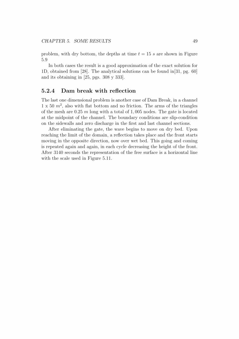
CHAPTER 5. SOME RESULTS 49
problem, with dry bottom, the depths at time t = 15 s are shown in Figure5.9
In both cases the result is a good approximation of the exact solution for1D, obtained from [28]. The analytical solutions can be found in[31, pg. 60]and its obtaining in [25, pgs. 308 y 333].
5.2.4 Dam break with reflection
The last one dimensional problem is another case of Dam Break, in a channel1 x 50 m2, also with flat bottom and no friction. The arms of the trianglesof the mesh are 0.25 m long with a total of 1, 005 nodes. The gate is locatedat the midpoint of the channel. The boundary conditions are slip-conditionon the sidewalls and zero discharge in the first and last channel sections.
After eliminating the gate, the wave begins to move on dry bed. Uponreaching the limit of the domain, a reflection takes place and the front startsmoving in the opposite direction, now over wet bed. This going and comingis repeated again and again, in each cycle decreasing the height of the front.After 3140 seconds the representation of the free surface is a horizontal linewith the scale used in Figure 5.11.

CHAPTER 5. SOME RESULTS 50200 0.1 0 0.1 0
0
0.1
0.2
0.3
0.4
0.5
0.6
0.7
0.8
0.9
1
1.1
0 50 100 150 200
Exacta Calculada
Figure 5.8: Dam break over wet bed. t = 25 s.
199 0 0 0 0200 0 0 0 0
0
0.1
0.2
0.3
0.4
0.5
0.6
0.7
0.8
0.9
1
1.1
0 50 100 150 200
Exacta Calculada
Figure 5.9: Dam break over dry bed. t = 15 s.

CHAPTER 5. SOME RESULTS 51
t=0 seg.
0
0.2
0.4
0.6
0.8
1
0 10 20 30 40 50
t=2.1 seg.
0
0.2
0.4
0.6
0.8
1
0 10 20 30 40 50
t=4 seg.
0
0.2
0.4
0.6
0.8
1
0 10 20 30 40 50
t=5.7 seg.
0
0.2
0.4
0.6
0.8
1
0 10 20 30 40 50
t=7.5 seg.
0
0.2
0.4
0.6
0.8
1
0 10 20 30 40 50
t=9.5 seg.
0
0.2
0.4
0.6
0.8
1
0 10 20 30 40 50
t=11.5 seg.
0
0.2
0.4
0.6
0.8
1
0 10 20 30 40 50
t=13.7 seg.
0
0.2
0.4
0.6
0.8
1
0 10 20 30 40 50
t=15.9 seg.
0
0.2
0.4
0.6
0.8
1
0 10 20 30 40 50
Figure 5.10: Dam Break with reflection 1.
t=18.2 seg.
0
0.2
0.4
0.6
0.8
1
0 10 20 30 40 50
t=20.8 seg.
0
0.2
0.4
0.6
0.8
1
0 10 20 30 40 50
t=23.8 seg.
0
0.2
0.4
0.6
0.8
1
0 10 20 30 40 50
t=26.6 seg.
0
0.2
0.4
0.6
0.8
1
0 10 20 30 40 50
t=29.3 seg.
0
0.2
0.4
0.6
0.8
1
0 10 20 30 40 50
t=32 seg.
0
0.2
0.4
0.6
0.8
1
0 10 20 30 40 50
t=49.7 seg.
0
0.2
0.4
0.6
0.8
1
0 10 20 30 40 50
t=3140 seg.
0
0.2
0.4
0.6
0.8
1
0 10 20 30 40 50
t=65.8 seg.
0
0.2
0.4
0.6
0.8
1
0 10 20 30 40 50
Figure 5.11: Dam Break with reflection 2.

CHAPTER 5. SOME RESULTS 52
5.3 Two dimensional problems
5.3.1 Partial Dam Break
Now a two-dimensional Dam Break problem is solved. The domain is nowsquare divided into two parts by a wall. The gap in the wall is partial andasymmetric. The domain is 200 x m2 with nodes every 5 m, with 1656computational nodes. There is no friction on the bottom and walls.
Two cases are solved with the following initial conditions of depth:
• Depth: upstream H1 = 10 m and downstream H0 = 5 m.
• Depth: upstream H1 = 5 m and downstream H0 = 0 m.
In Figure 5.12 a wavefront can be seen that, after a time t = 7.1 s, reachesthe right side of the contour. Figure 5.13 represents the velocity field. Thewavefront in Figure 5.14 is clearly different, due to dry bed condition. Finally(Figure 5.15) shows the mesh used in both cases.
6
8
10
H
0
50
100
150
200
X
050
100150
200
Y
XY
ZFrame 001 22 Apr 2004 ROTURA_P5 , DELTAT= .310000, N= 23Frame 001 22 Apr 2004 ROTURA_P5 , DELTAT= .310000, N= 23
Figure 5.12: 2D Dam Break. H1/H0 = 2. t = 7.1 s.
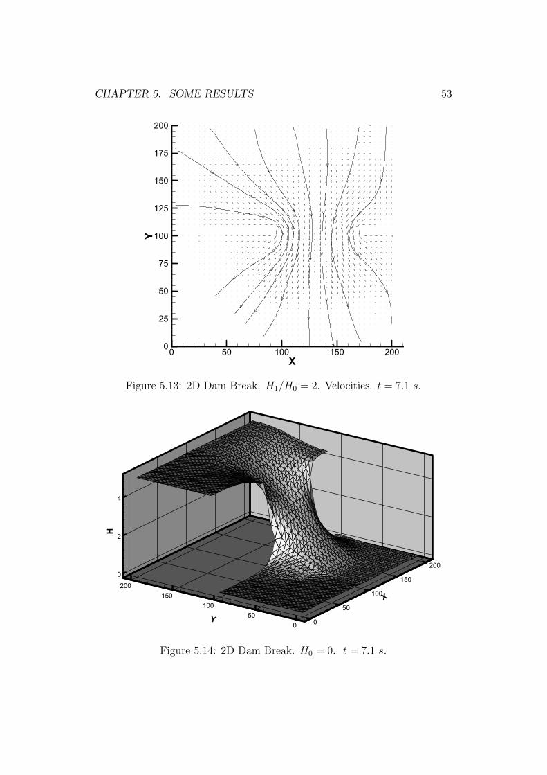
CHAPTER 5. SOME RESULTS 53
X
Y
0 50 100 150 2000
25
50
75
100
125
150
175
200
Frame 001 22 Apr 2004 ROTURA_P5 , DELTAT= .310000, N= 23Frame 001 22 Apr 2004 ROTURA_P5 , DELTAT= .310000, N= 23
Figure 5.13: 2D Dam Break. H1/H0 = 2. Velocities. t = 7.1 s.
0
2
4
H
0
50
100
150
200
X
050
100150
200
Y
XY
ZFrame 001 22 Apr 2004 ROTURA_P6 , DELTAT= .310000, N= 23Frame 001 22 Apr 2004 ROTURA_P6 , DELTAT= .310000, N= 23
Figure 5.14: 2D Dam Break. H0 = 0. t = 7.1 s.

CHAPTER 5. SOME RESULTS 54
X
Y
0 50 100 150 2000
25
50
75
100
125
150
175
200
Frame 001 22 Apr 2004 ROTURA_P5 , DELTAT= .310000, N= 23Frame 001 22 Apr 2004 ROTURA_P5 , DELTAT= .310000, N= 23
Figure 5.15: 2D Dam Break. Computational mesh.
X
Y
0.8 1 1.2 1.4 1.6 1.8 2 2.2 2.4
0
0.2
0.4
0.6
0.8
1
Frame 001 27 Apr 2004 EscalaPcs3,CICLO= 1,ITKE= 0,TIEMPO= 23.3137 TIEMKE= 0.0000,RNUCTE=0.000000Frame 001 27 Apr 2004 EscalaPcs3,CICLO= 1,ITKE= 0,TIEMPO= 23.3137 TIEMKE= 0.0000,RNUCTE=0.000000
Figure 5.16: Fishway. Computational mesh.
CHAPTER 5. SOME RESULTS 55
5.3.2 Flow in a fishway
A dam in a river is a barrier to the free movement of fish, which is particularlyimportant in the case of species that need to go upstream to spawn. To solvethis problem fishways can be used, but their slope is generally high, producingan excessive water velocity. It can be reduced by means of deflectors thatgenerate high energy dissipation, creating areas of low speed, where the fishcan rest during the climb.
In the Center for Technology Innovation in Building and Civil Engineering(CITEEC), University of A Coruna, measurements were made of depths andvelocities with two fishway designs for different slopes and discharges [26].The experimental setup consists of nine pools, four of each type with anintermediate of transition. The two types are shown in Figures 5.17 and5.18 and, in the first one, also the position of the measurement points. Theexperimental measurements for the different slopes and discharges analyzed,have been made in the pool 7, the third from the bottom. This is why thecomputational domain is a set of three pools, numbered 1 through 3 in thedirection of flow, to compare the values of the variables in the number 1 withthe experimental results.
The calculations have been performed for a slope of 5.7% and a dischargeof 24.6 l/s. The Manning coefficient is 0.015. Despite the steep slope andbecause of the action of the deflectors, the flow is subcritical. The boundarycondition of depth is imposed on the outlet section of pool 3, fixing in eachpoint of the section the depth obtained from the measurements.
Figure 5.16 shows the mesh used. In Figures 5.19 to 5.21 velocity vectors,velocity modules and depth values are shown. In the six following figures acomparison is made between the computational values obtained for the firstpool and the experimental values.

CHAPTER 5. SOME RESULTS 56
Figure 5.17: Fishway. Type I. Distances in cm.
Figure 5.18: Fishway. Type II. Distances in mm.

CHAPTER 5. SOME RESULTS 57
X
Y
0 0.5 1 1.5 2 2.5 3 3.5 4 4.50
0.5
1
Frame 001 27 Apr 2004 EscalaPcs3,CICLO= 1,ITKE= 0,TIEMPO= 23.3137 TIEMKE= 0.0000,RNUCTE=0.000000Frame 001 27 Apr 2004 EscalaPcs3,CICLO= 1,ITKE= 0,TIEMPO= 23.3137 TIEMKE= 0.0000,RNUCTE=0.000000
Figure 5.19: Fishway. Velocities.
X
Y
0 0.5 1 1.5 2 2.5 3 3.5 4 4.50
0.5
1
1.5VM: 0.05 0.125 0.2 0.275 0.35 0.425 0.5 0.575 0.65 0.725 0.8 0.875 0.95
Frame 001 27 Apr 2004 EscalaPcs3,CICLO= 1,ITKE= 0,TIEMPO= 23.3137 TIEMKE= 0.0000,RNUCTE=0.000000Frame 001 27 Apr 2004 EscalaPcs3,CICLO= 1,ITKE= 0,TIEMPO= 23.3137 TIEMKE= 0.0000,RNUCTE=0.000000
Figure 5.20: Fishway. Velocity modulus.
X
Y
0 0.5 1 1.5 2 2.5 3 3.5 4 4.50
0.5
1
1.5H: 0.165 0.17 0.175 0.18 0.185 0.19 0.195 0.2 0.205 0.21 0.215 0.22 0.225 0.23 0.235
Frame 001 27 Apr 2004 EscalaPcs3,CICLO= 1,ITKE= 0,TIEMPO= 23.3137 TIEMKE= 0.0000,RNUCTE=0.000000Frame 001 27 Apr 2004 EscalaPcs3,CICLO= 1,ITKE= 0,TIEMPO= 23.3137 TIEMKE= 0.0000,RNUCTE=0.000000
Figure 5.21: Fishway. Depths.

CHAPTER 5. SOME RESULTS 58
X
Y
0.8 1 1.2 1.4 1.6 1.8 2 2.2 2.4
0.2
0.4
0.6
0.8
Frame 001 27 Apr 2004 EscalaPcs3,CICLO= 1,ITKE= 0,TIEMPO= 23.3137 TIEMKE= 0.0000,RNUCTE=0.000000Frame 001 27 Apr 2004 EscalaPcs3,CICLO= 1,ITKE= 0,TIEMPO= 23.3137 TIEMKE= 0.0000,RNUCTE=0.000000
Figure 5.22: Fishway, pool 1. Computational velocities.
X
Y
0.8 1 1.2 1.4 1.6 1.8 2 2.2 2.4
0.2
0.4
0.6
0.8
Frame 001 27 Apr 2004 Frame 001 27 Apr 2004
Figure 5.23: Fishway, pool 1. Measured velocities.

CHAPTER 5. SOME RESULTS 59
X
Y
0.8 1 1.2 1.4 1.6 1.8 2 2.2 2.4
0.2
0.4
0.6
0.8VM0.950.8750.80.7250.650.5750.50.4250.350.2750.20.1250.05
Frame 001 27 Apr 2004 EscalaPcs3,CICLO= 1,ITKE= 0,TIEMPO= 23.3137 TIEMKE= 0.0000,RNUCTE=0.000000Frame 001 27 Apr 2004 EscalaPcs3,CICLO= 1,ITKE= 0,TIEMPO= 23.3137 TIEMKE= 0.0000,RNUCTE=0.000000
Figure 5.24: Fishway, pool 1. Computational velocity modulus.
X
Y
0.8 1 1.2 1.4 1.6 1.8 2 2.2 2.4
0.2
0.4
0.6
0.8VM0.950.8750.80.7250.650.5750.50.4250.350.2750.20.1250.05
Frame 001 19 Oct 2004 Frame 001 19 Oct 2004
Figure 5.25: Fishway, pool 1. Measured velocity modulus.

CHAPTER 5. SOME RESULTS 60
X
Y
1 1.2 1.4 1.6 1.8 2
0.2
0.4
0.6
0.8 H0.2350.230.2250.220.2150.210.2050.20.1950.190.1850.180.1750.170.165
Frame 001 27 Apr 2004 EscalaPcs3,CICLO= 1,ITKE= 0,TIEMPO= 23.3137 TIEMKE= 0.0000,RNUCTE=0.000000Frame 001 27 Apr 2004 EscalaPcs3,CICLO= 1,ITKE= 0,TIEMPO= 23.3137 TIEMKE= 0.0000,RNUCTE=0.000000
Figure 5.26: Fishway, pool 1. Computational depth.
X
Y
1 1.2 1.4 1.6 1.8 2
0.2
0.4
0.6
0.8 H0.2350.230.2250.220.2150.210.2050.20.1950.190.1850.180.1750.170.165
Frame 001 27 Apr 2004 Frame 001 27 Apr 2004
Figure 5.27: Fishway, pool 1. Measured depth.

References
[1] Alcrudo, F. (1992), Esquemas de alta resolucion de variacion total de-creciente para el estudio de flujos discontinuos de superficie libre, Tesisdoctoral, Universidad de Zaragoza.
[2] Alcrudo, F. & Garcıa-Navarro, P. (1993), A high resolution Godunovtype scheme in finite volumes for the 2D shallow-water equations, Inter-national Journal for Numerical Methods in Fluids 16, 489-505.
[3] Alcrudo, F. (2002), A state of the art review on mathematical model offlood propagation, Proceedings of the 1st IMPACT project workshop,HR Wallingford, UK, 16-17 May, 2002 (www.impact-project.net).
[4] Anderson, J.D.; Degrez, G.; Dick, E. & Grundmann, R. (1996), Com-putational fluid dynamics. An introduction, Wendt, J.F. (ed.), Springer.
[5] Bermudez, A.; Dervieux, A.; Desideri, J. & Vazquez, M.E. (1998), Up-wind schemes for the two dimensional shallow water equations with vari-able depth using unstructured meshes, Computer Methods in AppliedMechanics and Engineering 155, 49-72.
[6] Brigham Young University (1996), User´s guide to RMA2 version 4.3Salt Lake City, EEUU.
[7] Brufau, P. (2000), Simulacion bidimensional de flujos hidrodinamicostransitorios en geometrıas irregulares, Tesis doctoral, Universidad deZaragoza.
[8] Caleffi, V., Valiani, A. & Zanni, A. (2003), Finite volume method forsimulating extreme flood events in natural channels, Journal of HydraulicResearch, 41 , 2, 167-177.
[9] Chaudhry, M.H. (1993), Open channel flow, Prentice Hall, New Jersey.
[10] Chow, V.T. (1994), Hidraulica de canales abiertos, Mc Graw-Hill.
61

REFERENCES 62
[11] DHI Software (2001), MIKE 21: A modelling system for estuaries,coastal waters and seas, Danish Hydraulic Institute Water and Envi-ronment, Horsholm, Denmark.
[12] Donea, J. & Huerta, A. (2003), Finite element methods for flow prob-lems, John Wiley & Sons, Chichester, England.
[13] Eymard, R.; Gallouet, T. & Herbin, R. (1997), Finite volume methods,Prepublication n0 97-19 of LATP, umr 6632, Marseille. To appear inHandbook of Numerical Analysis, P.G. Ciarlet and J.L. Lions eds.
[14] Glaister, P. (1988), Approximate Riemann solutions of the shallow waterequations, Journal of Hydraulic Research 26, 3, 293-306.
[15] Godlewski, E & Raviart, P. (1996), Numerical approximation of hyper-bolic systems of conservation laws, Springer, Berlin.
[16] Harten, A.; Lax, P. & Van Leer, B. (1983), On upstream differencing andGodunov-type schemes for hyperbolic conservation laws, SIAM Rev. 25,35-61 (en Upwind and high-resolution schemes, Springer, Berlin 1997).
[17] Hirsch, C. (2000), Numerical computation of internal and external flows(Volume I. Fundamentals of numerical discretization), John Wiley &Sons, Chichester.
[18] Hirsch, C. (2000), Numerical computation of internal and external flows(Volume II. Computational methods for inviscid and viscous flows), JohnWiley & Sons, Chichester.
[19] Idelsohn, S.R. & Onate, E. (1993), Finite volumes and finite elements:two good friends, International Journal for Numerical Methods in Engi-neering 37, 19, 3323-3341.
[20] LeVeque, R. J. (2002), Finite volume methods for hyperbolic problems,Cambridge University Press.
[21] Lopez Pena, F. (2000), Mecanica de fluidos, Servicio de publicaciones,Universidad de A Coruna.
[22] Peraire, J. (1986), A finite element method for convection dominatedflows, Ph.D. Thesis, University College of Swansea.
[23] Roe, P.L. (1981), Approximate Riemann solvers, parameter vectors anddifference schemes, Journal of Computational Physics, 43, 357-372.

REFERENCES 63
[24] Smagorinsky, J. (1963), General circulation experiments with the prim-itive equations, part I: the basic experiment, Monthly Weather Review91, 99-164.
[25] Stoker, J.J. (1992), Water waves. The mathematical theory with appli-cations, John Wiley & Sons, New York.
[26] Teijeiro, T. (2001), Criterios de diseno de escalas de peces de hendiduravertical, Tesis doctoral, Universidad de Santiago de Compostela.
[27] Toro, E.F. (1997), Riemann solvers and numerical methods for fluiddynamics. A practical introduction, Springer, Berlin.
[28] Toro, E.F. (2000), Numerica. A library of source codes for teaching,research and applications, Numeritek Ltd., Cheshire.
[29] Toro, E.F. (2001), Shock-capturing methods for free-surface shallowflows, John Wiley & Sons, Chichester.
[30] Van Leer, B. (1977), Towards the ultimate conservative differencescheme III. Upstream-centered finite-difference schemes for ideal com-pressible flow, Journal of Computational Physics 23, 263-275.
[31] Vazquez Cendon, M.E. (1994), Estudio de esquemas descentrados parasu aplicacion a las leyes de conservacion hiperbolicas con terminosfuente, Tesis doctoral, Universidad de Santiago de Compostela.
[32] Vazquez Cendon, M.E. (1999), Improved treatment of source terms inupwind schemes for the shallow water equations in channels with irreg-ular geometry, Journal of Computational Physics 148, 497-526.
[33] Wright, N. (2001), Conveyance implications for 2-D and 3-D modelling.Scoping study for reducing uncertainty in river flow conveyance, HRWallingford.
[34] Zienkiewicz, O.C. & Heinrich, J.C. (1979), A unified treatment of steady-state shallow water and two dimensional Navier-Stokes equations. Finiteelement penalty function approach, Computer Methods in Applied Me-chanics and Engineering 17/18, 673-698.
[35] Zienkiewicz, O.C. & Onate, E. (1990), Finite volumes vs. finite elements.Is there really a choice?, CIMNE, Barcelona.