Observational constraints from the Solar System

and fromExtrasolar Planets

Lecture 1 Part II

Lecture Universität Heidelberg WS 11/12Dr. Christoph Mordasini

mordasini@mpia.de Mentor Prof. T. Henning

Lecture overview

1. Introduction

2. Planet formation paradigm

3. Structure of the Solar System

4. The surprise: 51 Peg b

5. Detection techniques: radial velocity, transits, direct imaging, (microlensing, timing, astrometry)

6. Properties of extrasolar planets: mass, distance, eccentricity distributions, metallicity effect, mass-radius diagram, ...

6. Properties of extrasolar planets

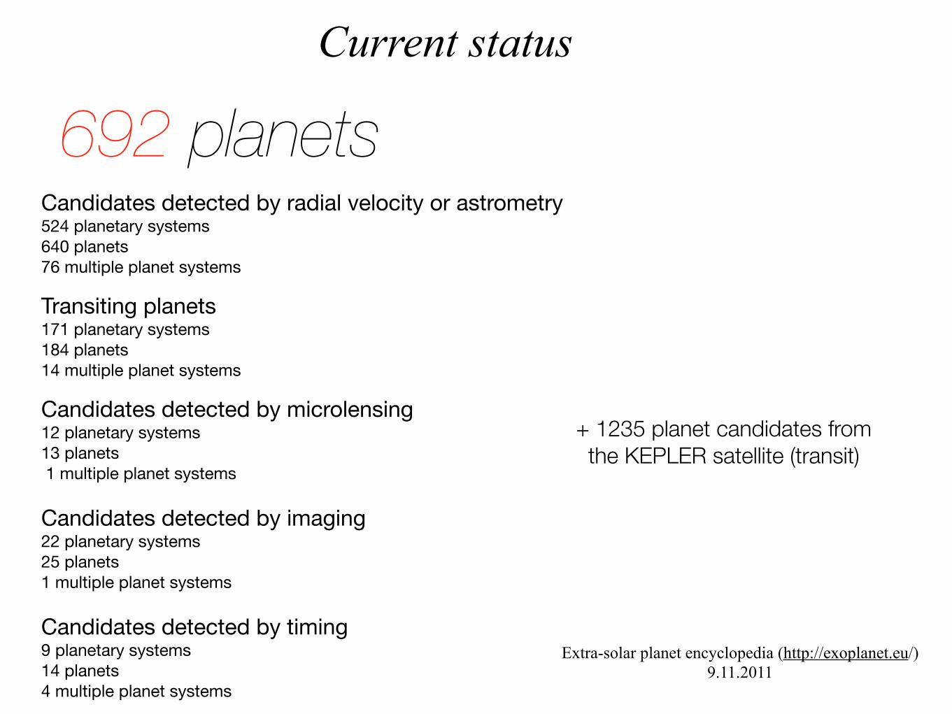
Current status

 692 planetsCandidates detected by radial velocity or astrometry524 planetary systems640 planets76 multiple planet systems

Transiting planets171 planetary systems184 planets14 multiple planet systems

Candidates detected by microlensing12 planetary systems13 planets 1 multiple planet systems

Candidates detected by imaging22 planetary systems25 planets1 multiple planet systems

Candidates detected by timing9 planetary systems14 planets4 multiple planet systems

+ 1235 planet candidates from the KEPLER satellite (transit)

Extra-solar planet encyclopedia (http://exoplanet.eu/)9.11.2011

direct imaging

Different techniques - different constraints

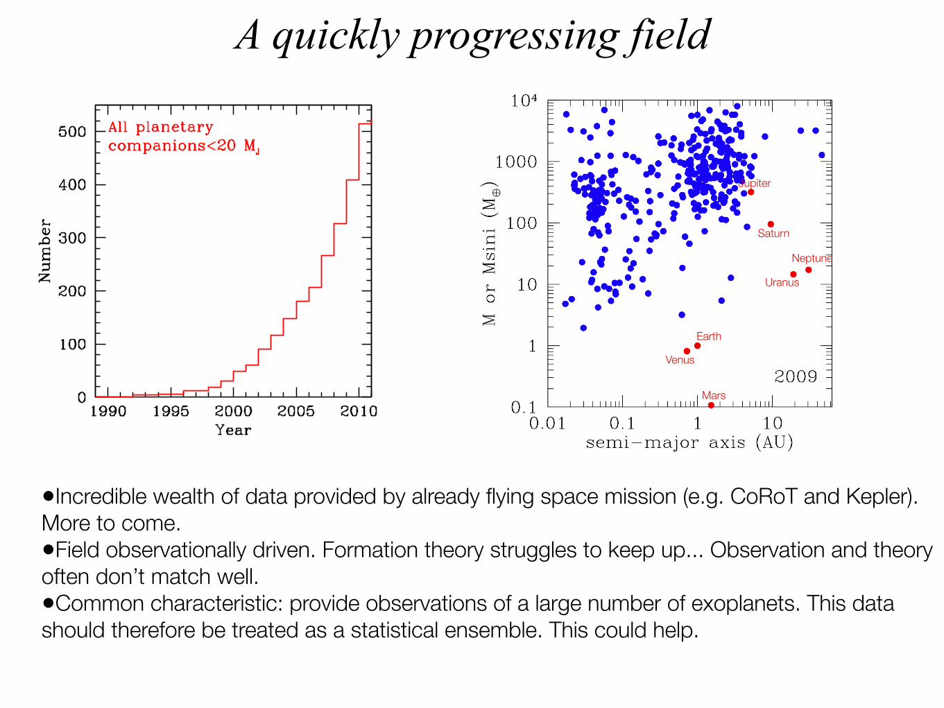
•Incredible wealth of data provided by already flying space mission (e.g. CoRoT and Kepler). More to come.•Field observationally driven. Formation theory struggles to keep up... Observation and theory often don’t match well.•Common characteristic: provide observations of a large number of exoplanets. This data should therefore be treated as a statistical ensemble. This could help.

A quickly progressing field

Venus

Earth

Uranus

Neptune

Saturn

Jupiter

Mars

• Giant planet frequency and host star [Fe/H] are positively correlated.

• Extrasolar planets exhibit a very large diversity (all techniques).• Frequencies -Low mass close-in planets: approx. 50 % (radial velocity)

-Jovian planets inside a few AU: approx. 10-15 % (rv)-Hot Jupiters: 0.5-1% (rv, transits)-Cold Neptunes are common (microlensing)-Overall (FGK stars): any mass, P<10 years: 75% (rv)

• The mass function is strongly rising towards small masses. There might be local minimum in the planetary mass function around 30-100 Mearth (rv).

• The radius distribution is strongly increasing towards small radii (transits).

• The semimajor axis distribution of giant planets consists of a pile up at a period of about 3 days, a period valley, and an upturn at about 1 AU. (rv)• Close-in low mass (or small radius) planets are found somewhat further out than Hot Jupiters (rv, transits).

• Hot Jupiters are lonely (rv, transits).

• Low mass close-in planets are in multiple systems (rv, transits).

• Massive giants planets at large distances are rare, at least around solar like stars (direct imaging).

Overview on observed exoplanet properties

Today, formation theory cannot explain all th

ese

observed characteristics in one coherent picture.

But at least for so

me observations, theory can give us

ideas about possible mechanisms responsible for them.

6.1 a-M diagram

Diversity & structures in the a-M diagram

Diversity - close-in giant planets - evaporating planets - eccentric planets

- super Jupiters- Hot Neptunes & Super Earth- pile-ups and voids:

planetary desertperiod valley

- planets at large distances

J. Schneider’s exoplanet.eu~2010 (already outdated!)

Direct imaging

Microlensing

Radial velocity& Transits

HARPS high precision sample 2011

Frequency of planet types

Bias-corrected frequency (at least one planet per star) in the a-M (or equivalently period-mass) plane found by high precision RV around solar like FGK stars.

Close in planets: P<50 d

Mayor et al. 2011

6.2 Mass distribution

4 Marcy, Butler, Fischer, Vogt, Wright, Tinney and Jones

The target list also includes 120 M dwarfs, located mostly within 10 pc withdeclination north of !30 deg.87) For the late-type K and M dwarfs, we restrictedour selection to stars brighter than V = 11. All slowly rotating stars are surveyedwith a Doppler precision of 3 m s!1 to provide a uniform sensitivity to planets. Thusfar, our Lick, Keck, and Anglo-Australian surveys have revealed 104 planets orbiting88 stars, including 12 multi-planet systems. The orbital elements and masses of theseexoplanets are regularly updated at: http://exoplanets.org .

§3. Observed properties of exoplanets

We derive the statistical properties of planets from the 1330 FGKM target starsfor which we have uniform precision of 3 m s!1 and at least 6 years duration ofobservations. Detected exoplanets have minimum masses, Msin i, between 6 MEarth

and "15 MJup, with an upper mass limit corresponding to the (vanishing) tail ofthe mass distribution. The planet mass distribution is shown in Fig. 1 and followsa power law, dN/dM # M!1.05 54), 55) a!ected very little by the unknown sin i.41)

The paucity of companions with Msin i greater than 12 MJup confirms the presenceof a “brown dwarf desert”54) for companions with orbital periods up to a decade.

Planet Mass Distribution

0 2 4 6 8 10 12 14 M sin i (MJUP)

0

5

10

15

20

Nu

mb

er

of

Pla

ne

ts

dN/dM ! M !1.05

Keck, Lick, AAT

104 Planets

Fig. 1. The histogram of 104 planet masses (Msin i) found in the uniform 3 m s!1 Doppler surveyof 1330 stars at Lick, Keck, and the AAT telescopes. The bin size is 0.5 MJup. The distributionof planet masses rises as M!1.05 from 10 MJup down to Saturn masses, with incompleteness atlower masses.

Marcy et al. 2005

Mass distribution: old versions (giants)

•mass distribution from RV observations.•rising towards smaller masses. No obs. bias: smaller masses are more difficult to detect.•beware of uncorrected (biased) distributions! •frequency of Jovian planets falls as about M-1.•maximum of giant planet masses at about 1 Jupiter mass.•HARPS gave around 2007 the first hint of a second population of low mass planets.

HARPS

?

Udry et al. 2007

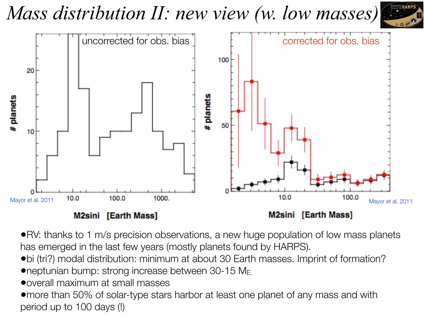
Mass distribution II: new view (w. low masses)

•RV: thanks to 1 m/s precision observations, a new huge population of low mass planets has emerged in the last few years (mostly planets found by HARPS).•bi (tri?) modal distribution: minimum at about 30 Earth masses. Imprint of formation?•neptunian bump: strong increase between 30-15 ME. •overall maximum at small masses•more than 50% of solar-type stars harbor at least one planet of any mass and with period up to 100 days (!)

uncorrected for obs. bias corrected for obs. bias

Mayor et al. 2011Mayor et al. 2011

• less than 0.6 % of Sun-like stars have a brown-dwarf companion: so called “Brown dwarf desert”•mass distribution function shows a lack of objects between 25-45 MJ. Upper end of planet mass distribution?•Nothing particular is seen at 13 MJ (D-burning limit).

Mass distribution III: upper boundarySahlmann et al. 2010

A distinction of BD vs. planets based on formation seems advisable, but difficult to realize in practice.

Segresan et al.

desert

Grether & Lineweaver 2006

6.3 Semimajor axis distribution

Semimajor axis distribution I: giants

The semimajor axis distribution of giant planets found by RV consists of a •pile up at a period of about 3 days (0.04 AU). Stopping mechanism for migration? Tidal circularization? Magnetospheric cavity?

•maybe this pile up is only tiny, when properly correcting for obs. bias...•a period valley (10 d < P < 100 d). Timescale effect?•an upturn at about 1 AU. Reservoir at large distances. Original formation region?

ANRV320-AA45-10 ARI 27 July 2007 19:32

2.3. Orbital Period Distribution of ExoplanetsThe distribution of periods of giant exoplanets is basically made of two main fea-tures (Figure 4): a peak around 3 days plus an increasing distribution with period(Cumming, Marcy & Butler 1999, Udry, Mayor & Santos 2003, Marcy et al. 2005).The hot Jupiters were completely unexpected before the first exoplanet discoveries.The standard model (e.g., Mizuno 1980, Pollack et al. 1996, Rice & Armitage 2003)suggests that giant planets form first from ice grains in the outer region of the sys-tem where the temperature of the stellar nebula is cool enough. Such grain growthprovides the supposed requisite solid core around which gas could rapidly accrete(Safronov 1969) over the lifetime of the protoplanetary disk (!107 year, e.g., Haisch,Lada & Lada 2001). During this process, they are also supposed to undergo a migra-tion process moving them from their birth place close to the central star (see, e.g.,Lin, Bodenheimer & Richardson 1996; Ward 1997; Papaloizou & Terquem 2006),where they have to stop before falling onto the star. Several stopping mechanismshave been proposed, invoking, e.g., a magnetospheric central cavity of the accretiondisk, tidal interactions with the host stars, Roche-lobe overflow by the young inflatedgiant planet, or photoevaporation. The question is, however, still debated. Alter-native points of view invoke in situ formation (Bodenheimer, Hubickyj & Lissauer2000), possibly triggered through disk instabilities (Boss 1997, Durisen et al. 2007).Note however that, even in such cases, subsequent disk-planet interactions leading to

N

log(Period) (days)

20

15

10

5

0

1 2 3

Figure 4Period distribution ofknown gaseous giant planetsdetected by radial-velocitymeasurements and orbitingdwarf primary stars (openhistogram). The redhatched part of thehistogram represents lightplanets with m2 sin i "0.75 MJup that probablyhave migrated toward thecenter of the system. Forcomparison, the perioddistribution of knownNeptune-mass planets (withshort periods and masses"21 M#) is given by theblue filled histogram,showing a flatterdistribution with periods upto 30 days. (Note, however,that there is still very highobservationalincompleteness for theselow-mass planets).

408 Udry · Santos

Annu. R

ev. A

stro

. A

stro

phys.

2007.4

5:3

97-4

39. D

ow

nlo

aded

fro

m a

rjourn

als.

annual

revie

ws.

org

by U

niv

ersi

ty o

f B

ern o

n 1

0/0

8/0

7. F

or

per

sonal

use

only

.

Udry & Santos 2007

Msini>0.75 MJ Msini<0.75 MJMsini<21 Mearth

uncorrected for obs. bias

Msini>50 Mearth

uncorrected for obs. biascorrected for obs. bias

Mayor et al. 2011

Semimajor axis distribution II: low mass/radius planets

Cut off below P0: -small radii 2-4 Re: P0 = 7 days-large radii >4 Re : P0 = 2 days.

Neptunian and smaller sized further out than giant planets. No pile up at 3 days. Consistent with earlier results from high precision RV. Lovis et al. 2009 estimated 10 days. Different stopping mechanism?

Planet Occurrence from Kepler 13

TABLE 4Planet Occurrence for GK Dwarfs

Rp(R!) P < 10 days P < 50 days

2–4 R! 0.025± 0.003 0.130± 0.008

4–8 R! 0.005± 0.001 0.023± 0.003

8–32 R! 0.004± 0.001 0.013± 0.002

2–32 R! 0.034± 0.003 0.165± 0.008

TABLE 5Best-fit Parameters of Cutoff Power Law Model

Rp kP ! P0 "(R!) (days)

2–4 R! 0.064 ± 0.040 0.27 ± 0.27 7.0± 1.9 2.6± 0.3

4–8 R! 0.0020 ± 0.0012 0.79 ± 0.50 2.2± 1.0 4.0± 1.2

8–32 R! 0.0025 ± 0.0015 0.37 ± 0.35 1.7± 0.7 4.1± 2.5

2–32 R! 0.035 ± 0.023 0.52 ± 0.25 4.8± 1.6 2.4± 0.3

corrected for incompleteness.The occurrence distributions in the top panel of Figure

6 have shapes that are more complicated than simplepower laws. Occurrence falls o! rapidly at short periods.We fit each of these distributions to a power law with anexponential cuto!,

df(P )

d logP= kPP

!!

1! e!(P/P0)!"

. (8)

This function behaves like a power law with exponent! and normalization kP for P " P0. For periods P(in days) near and below the cuto! period P0, f(P ) fallso! exponentially. The sharpness of this transition is gov-erned by ". Thus the parameters of equation (8) measurethe slope of the power law planet occurrence distributionfor “longer” orbital periods as well as the transition pe-riod and sharpness of that transition.We fit equation (8) to the four ranges of radii shown

in Figure 6 (top panel) and list the best-fit parame-ters in Table 5. We note that ! > 0 for all planetradii considered, i.e. planet occurrence increases withlogP . For the largest planets (Rp = 8–32 R"), != 0.37 ± 0.35 is consistent with the power law occur-rence distribution derived by Cumming et al. (2008) forgas giant planets with periods of 2–2000 days, df #M!0.31±0.2P 0.26±0.1 d logM d logPP0 and " can be interpreted as tracers of the migration

and stopping mechanisms that deposited planets at theclosest orbital distances. With decreasing planet radius,P0 increases and " decreases, shifting the cuto! periodoutward and making the transition less sharp. Thus,gas giant planets (Rp = 8–32 R") on average migratecloser to their host stars (P0 is small) and the stoppingmechanism is abrupt (" is large). On the other hand,the smallest planets in our study have a distribution oforbital distances (and periods) with a characteristic stop-ping distance farther out and a less abrupt fall-o! close-in.The normalization constant kP is highly correlated

with the other parameters of equation (8). A more ro-bust normalization is provided by the requirement that

0.68 1.2 2.0 3.4 5.9 10 17 29 50Orbital Period (days)

0.0001

0.0010

0.0100

0.1000

Nu

mb

er

of

Pla

ne

ts p

er

Sta

r P0 =

7.0

days

P0 =

2.2

days

P0 =

1.7

days

2!4 RE

4!8 RE

8!32 RE

0.68 1.2 2.0 3.4 5.9 10 17 29 50

0.0001

0.0010

0.0100

0.1000

Fig. 7.— Measured planet occurrence (filled circles) as a func-tion of orbital period with best-fit models (solid curves) overlaid.These models are power laws with exponential cuto!s below a char-acteristic period, P0 (see text and equation 8). P0 increases withdecreasing planet radius, suggesting that the migration and park-ing mechanism that deposits planets close-in depends on planetradius. Colors correspond to the same ranges of radii as in Figure6. The occurrence measurements (filled circles) are the same as inFigure 6, however for clarity the 2–32 R! measurements and fitare excluded here. As before, only stars in the solar subset (Table1) and planets with Rp > 2 R! were used to compute occurrence.

the integrated occurrence to P = 50 days is given inTable 4.

4. STELLAR EFFECTIVE TEMPERATURE

4.1. Planet Occurrence

In the previous section we considered only GK starswith properties consistent with those listed in Table 1.In particular, only stars with Te! = 4100–6100 K wereused to compute planet occurrence. Here we expand thisrange to 3600–7100 K and measure occurrence as a func-tion of Te! . This expanded set includes stars as cool asM0 and as hot as F2. For Te! outside of this range thereare too few stars to compute occurrence with reasonableerrors. We use the same cuts on brightness (Kp < 15)and gravity (log g = 4.0–4.9) as before. We also used thephotometric noise #CDPP values (as before) to computethe fraction of target stars around which each detectedplanet could have been detected with SNR$ 10. This en-sures that planet detectability down to sizes of 2 R" willbe close to 100%, for all of these included target starsindependent of their Te! .We computed planet occurrence using the same tech-

niques as in the previous section, namely equation (2).We subdivided the stars and their associated planets into500 K bins of Te! . We further subdivided the sample byplanet radius, considering di!erent ranges of Rp (2–4, 4–8, 8–32, and 2–32 R") separately. In summary, we com-puted planet occurrence as a function of Te! for severalranges of Rp and in all cases we considered all planetswith P < 50 days.Figure 8 shows these occurrence measurements as a

function of Te! . Most strikingly, occurrence is inverselycorrelated with Te! for small planets with Rp = 2–4 R".Fitting the occurrence of these small planets in the Te!bins shown in Figure 8, we find that a model linear in

Howard et al. 2011

Transits

The semimajor axis distribution of low mass planets found by RV consists of a •continuous increase to about 40 d. •then again a decrease. Why?

•affected by obs. bias? In principle corrected...•such planets seem extremely abundant.

RV Msini<50 Mearthuncorrected for obs. biascorrected for obs. bias

Mayor et al. 2011

6.4 Eccentricity distribution

Eccentricity distribution

•high and even very high eccentricities are common among exoplanets. This is very different than in the Solar System.•mean eccentricity for giants: 0.28 > any planet of the Solar System.•lower mass planets seem to have lower (but still quite high) e <0.5.•planets very close to the star get tidally circularized. •origin? formation - evolution?•several possible explanations: Planet-planet interactions, influence of stellar or planet companion (Kozai effect), planet-disk interaction (M >10 MJ), dynamical interactions in a cluster

Mayor et al. 2011

6.5 Metallicity

Stellar metallicity

•[Fe/H]: iron content of the star ([Fe/H]=0: solar composition, [Fe/H]=0.5: ~ 3 times more iron than the sun).•Iron serves as a proxy for the overall metal content in the star (scaled solar composition).•Stars in the the solar neighborhood have a distribution of metallicities which is roughly Gaussian around zero.•Other parts in the galaxies can have completely different [Fe/H] distributions. These stars can also have a non-scaled solar composition (e.g. thick disk stars).•There exists also a galactic metallicity gradient (higher [Fe/H] towards the center).

Mordasini et al. 2009

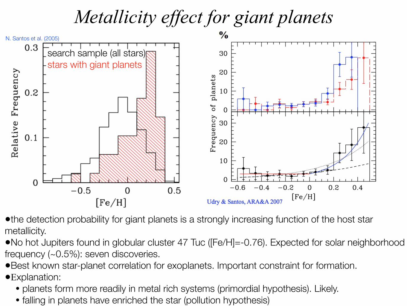
Metallicity effect for giant planets

•the detection probability for giant planets is a strongly increasing function of the host star metallicity.•No hot Jupiters found in globular cluster 47 Tuc ([Fe/H]=-0.76). Expected for solar neighborhood frequency (~0.5%): seven discoveries. •Best known star-planet correlation for exoplanets. Important constraint for formation.•Explanation:

• planets form more readily in metal rich systems (primordial hypothesis). Likely. • falling in planets have enriched the star (pollution hypothesis)

N. Santos et al. (2005)

search sample (all stars)stars with giant planets

No metallicity effect for low mass planets

•HARPS high precision sample: [Fe/H] for giant gaseous planets (black), for planets less massive than 30 ME (red), and for the global combined sample stars (blue). •No metallicity effect for low mass planets.•Even absence of low mass planets at high [Fe/H]?•Natural outcome in the core accretion formation model.

?

?

Mayor et al. 2011Mayor et al. 2011

Metallicity effect as function of mass

•The division between metalophile and not metalophile planets coincides with a minimum in the planetary mass function. (ca. 30 ME)•Different populations: Giant planets (w. gas runaway accretion) vs. Neptunian planets.

•Correlation with other elemental abundances in the stars are less clear (maybe Lithium-planet anticorrelation).

Sousa et al. 2011

6.6 Stellar mass

Influence of the host star mass

•Equal bin in log(Mstar)• M dwarfs • solar stars • intermediate masses

•Planetary system mass / star number=> mass of planetary material scales with Mstar

•Planets around more massive stars are more massive and more frequent.

•RV bias underestimate the last bin.

•The Neptunian vs Jovian planet ratio is higher around M dwarfs.

•Consistent with a correlation of stellar mass, protoplanetary disk mass, and (giant) planet formation probability.

6.7 Multiplicity

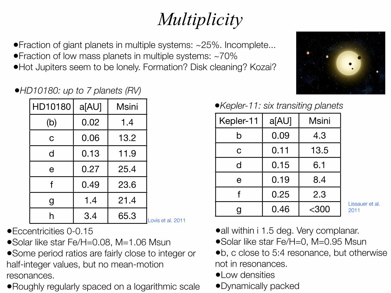
Multiplicity•Fraction of giant planets in multiple systems: ~25%. Incomplete...•Fraction of low mass planets in multiple systems: ~70%•Hot Jupiters seem to be lonely. Formation? Disk cleaning? Kozai?

•HD10180: up to 7 planets (RV)

HD10180 a[AU] Msini

(b) 0.02 1.4

c 0.06 13.2

d 0.13 11.9

e 0.27 25.4

f 0.49 23.6

g 1.4 21.4

h 3.4 65.3

•Eccentricities 0-0.15•Solar like star Fe/H=0.08, M=1.06 Msun•Some period ratios are fairly close to integer or half-integer values, but no mean-motion resonances.•Roughly regularly spaced on a logarithmic scale

Lovis et al. 2011

Kepler-11 a[AU] Msini

b 0.09 4.3

c 0.11 13.5

d 0.15 6.1

e 0.19 8.4

f 0.25 2.3

g 0.46 <300

•all within i 1.5 deg. Very complanar. •Solar like star Fe/H=0, M=0.95 Msun•b, c close to 5:4 resonance, but otherwise not in resonances.•Low densities•Dynamically packed

•Kepler-11: six transiting planets

Lissauer et al. 2011

Packed systemsnumbers=distance in mutual Hill spheres.

•Low mass planets seem to follow a radius exclusion law: they cannot be too close together when measured in mutual Hill spheres. •Many systems seem to be dynamically packed. Could not add another planet.•Numerical simulations show that systems with 3–5 planets and masses between a few ME and a few MJ, separations between adjacent planets should be of at least 7–9 mutual Hill radii to ensure stability on a 10-Gyr timescale.•Additional stability islands exist at resonances.•Dynamical evolution of the systems. Ejection/collision of surplus planets.

Lovis et al. 2011

•Kepler has detected a lot of systems with multiple transiting planet candidates.

Kepler multiple systems

•The distribution of observed period ratios shows that the majority of candidate pairs are neither in nor near low-order mean motion resonances.

•Nonetheless, there is a small but statistically significant excesses of pairs both in resonance and spaced slightly further apart, particularly near 2:1.

•Resonant capture due during migration?

– 45 –

1 1.5 2 2.5 3 3.5 4 4.5 50

1

N/N

TO

T <

5

Period Ratio

1 1.5 2 2.5 3 3.5 4 4.5 5

Kepler adjacent pairings

RV adjacent pairings

1 10 100 0

0.2

0.4

0.6

0.8

1N

/NT

OT

Period Ratio

Kepler adjacent pairings

RV adjacent pairings

Fig. 6.— Cumulative fraction of neighboring planet pairs for Kepler candidate multiplanet systems

with period ratio exceeding the value specified (solid curve). The cumulative fraction for neigh-

boring pairs in multiplanet systems detected via radial velocity is also shown (dashed curve), and

includes data from exoplanets.org as of 29 January 2011. (a) Linear horizontal axis, as in Figure 5.

The data are normalized for the number of adjacent pairs with P < 5, which equals 207 for the

Kepler candidates and 28 for RV planets. (b) Logarithmic horizontal axis. All 238 Kepler pairs are

shown; the three RV pairs with P > 200 are omitted from the plot, but used for the calculation of

Ntot, which is equal to 61.

– 46 –

1 1.5 2 2.5 3 3.5 4 4.5 50

50

100

150

200

250

300

350

400

450

500

Period Ratio

Slo

pe o

f C

um

ula

tive P

eriod R

atio

Kepler adjacent pairings

RV adjacent pairings

Fig. 7.— Slope of the cumulative fraction of Kepler neighboring planet pairs (solid black curve) and

multiplanet systems detected via radial velocity (dashed red curve) with period ratio exceeding the

value specified. The slope for theKepler curve was computed by taking the di!erence in period ratio

between points with N di!ering by 4 and dividing by 4. The slope for the RV curve was computed

by taking the di!erence in period ratio between points with N di!ering by 3 and dividing by 3,

and then normalizing by multiplying the value by the ratio of the number of Kepler pairings to

the number of radial velocity pairings (3.9). The spikes show excess planets piling up near period

commensurabilities.

Lissauer et al. 2011

6.8 Radius distribution

Planet Occurrence from Kepler 9

0.68 1.2 2.0 3.4 5.9 10 17 29 50Orbital Period, P (days)

1

2

4

8

16

32

Pla

ne

t R

ad

ius,

Rp (

RE)

0.000260.0075

304463 (10)

0.000090.0026

526181 (5)

0.000070.0021

579071 (4)

0.000040.0010

580181 (2)

0.000400.011

225401 (10)

0.000420.012

491703 (17)

0.000370.011

566653 (21)

0.000100.0029

579821 (6)

0.000100.0029

580091 (6)

0.000190.0054

580312 (11)

0.00230.067

154454 (50)

0.00210.060

4405911 (85)

0.00110.032

559667 (64)

0.000350.010

574423 (20)

0.000780.022

578084 (45)

0.000150.0044

579671 (9)

0.000580.017

580044 (34)

0.000670.019

580284 (39)

0.000150.0042

580361 (9)

0.00770.22

97646 (59)

0.00790.22

3727819 (262)

0.00510.15

5458521 (269)

0.00180.052

572629 (104)

0.000300.0087

577492 (18)

0.00120.036

579427 (73)

0.000430.012

579983 (25)

0.00120.034

580226 (69)

0.00220.062

57841 (18)

0.00560.16

2949811 (159)

0.0100.30

5226031 (521)

0.00620.18

5700121 (353)

0.00100.030

576534 (60)

0.00130.037

579034 (74)

0.000270.0076

579881 (15)

0.000250.0071

580171 (15)

0.0280.81

31703 (85)

0.0150.43

2160616 (375)

0.0190.53

4863936 (893)

0.0110.31

5660523 (607)

0.00270.076

575385 (153)

0.000530.015

578592 (31)

0.00120.034

579813 (70)

0.000490.014

580091 (28)

0.000260.0075

580301 (15)

0.0330.95

16052 (41)

0.0290.83

1471212 (410)

0.0280.79

4331834 (1101)

0.0110.30

5583416 (591)

0.00360.10

574296 (208)

0.00280.079

578044 (160)

0.00260.076

579634 (154)

0.000430.012

580041 (25)

0.0270.76

91577 (295)

0.0210.61

3629618 (749)

0.0150.43

5437117 (799)

0.00350.099

572405 (198)

0.00480.14

577385 (278)

0.00290.082

579973 (168)

0.000900.026

580201 (52)

0.68 1.2 2.0 3.4 5.9 10 17 29 50

1

2

4

8

16

32

0.001 0.002 0.004 0.0079 0.016 0.032 0.063 0.13 0.25 0.50 1.0

0.000035 0.00007 0.00014 0.00028 0.00056 0.0011 0.0022 0.0044 0.0088 0.018 0.035

Planet Occurrence ! d2f/dlogP/dlogRp

Planet Occurrence ! fcell

Fig. 4.— Planet occurrence as a function of planet radius and orbital period for P < 50 days. Planet occurrence spans more than threeorders of magnitude and increases substantially for longer orbital periods and smaller planet radii. Planets detected by Kepler havingSNR > 10 are shown as black dots. The phase space is divided into a grid of logarithmically spaced cells within which planet occurrenceis computed. Only stars in the “solar subset” (see selection criteria in Table 1) were used to compute occurrence. Cell color indicatesplanet occurrence with the color scale on the top in two sets of units, occurrence per cell and occurrence per logarithmic area unit. Whitecells contain no detected planets. Planet occurrence measurements are incomplete and likely contain systematic errors in the hatchedregion (Rp < 2 R!). Annotations in white text within each cell list occurrence statistics: upper left—the number of detected planetswith SNR > 10, npl,cell, and in parentheses the number of augmented planets correcting for non-transiting geometries, npl,aug,cell; lowerleft—the number of stars surveyed by Kepler around which a hypothetical transiting planet with Rp and P values from the middle of thecell could be detected with SNR > 10; lower right—fcell, planet occurrence, corrected for geometry and detection incompleteness; upperright—d2f/d log10 P/d log10 Rp, planet occurrence per logarithmic area unit (d log10 P d log10 Rp = 28.5 grid cells).

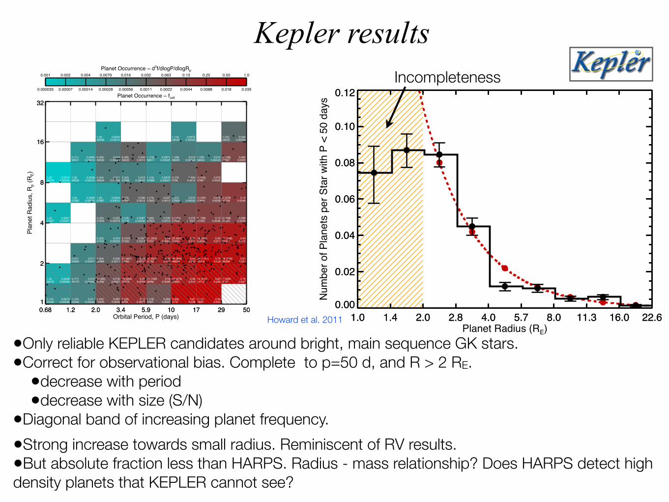
•Only reliable KEPLER candidates around bright, main sequence GK stars.•Correct for observational bias. Complete to p=50 d, and R > 2 RE.

•decrease with period•decrease with size (S/N)

•Diagonal band of increasing planet frequency.

Planet Occurrence from Kepler 11

Lissauer et al. (2011b) noted that the multi-planet sys-tems observed by Kepler have relatively low mutual incli-nations (typically a few degrees) suggesting a significantcorrelation of inclinations. Converting our measurementsof the mean number of planets per star to the fraction ofstars having at least one planet requires an understand-ing of the underlying multiplicity and inclination distri-butions. Such an analysis is attempted by Lissauer et al.(2011b), but is beyond the scope of this paper.It is worth identifying additional sources of error and

simplifying assumptions in our methods. The largestsource of error stems directly from 35% rms uncertaintyin R! from the KIC, which propagates directly to 35%uncertainty in Rp. We assumed a central transit overthe full stellar diameter in equation (2). For randomlydistributed transiting orientations, the average durationis reduced to !/4 times the duration of a central transit.Thus, this correction reduces our SNR in equation (1) bya factor of

!

!/4, i.e. a true signal-to-noise ratio thresh-old of 8.8 instead of 10.0. This is still a very conservativedetection threshold. Additionally, our method does notaccount for the small fraction of transits that are graz-ing and have reduced significance. We assumed perfect!t scaling for "CDPP values computed for 3 hr intervals.

This may underestimate "CDPP for a 6 hr interval (ap-proximately the duration of a P = 50 day transit) by"10%. These are minor corrections and a!ect the nu-merator and denominator of equation (2) nearly equally.

3.1. Occurrence as a Function of Planet Radius

Planet occurrence varies by three orders of magnitudein the radius-period plane (Figure 4). To isolate the de-pendence on these parameters, we first considered planetoccurrence as a function of planet radius, marginalizingover all planets with P < 50 days. We computed oc-currence using equation (2) for cells with the ranges ofradii in Figure 4 but for all periods less than 50 days.This is equivalent to summing the occurrence values inFigure 4 along rows of cells to obtain the occurrence forall planets in a radius interval with P < 50 days. Theresulting distribution of planet radii (Figure 5) increasessubstantially with decreasing Rp.We modeled this distribution of planet occurrence with

planet radius as a power law of the form

df(R)

d logR= kRR

". (4)

Here df(R)/d logR is the mean number of planets hav-ing P < 50 days per star in a log10 radius interval cen-tered on R (in R!), kR is a normalization constant, and# is the power law exponent. To estimate these param-eters, we used measurements from the 2–22.7 R! binsbecause of incompleteness at smaller radii and a lack ofplanets at larger radii. We fit equation (4) using a max-imum likelihood method (Johnson et al. 2010). Each ra-dius interval contains an estimate of the planet fraction,Fi = df(Ri)/d logR, based on a number of planet de-tections made from among an e!ective number of targetstars, such that the probability of Fi is given by the bi-nomial distribution

p(Fi|npl, nnd) = Fnpl

i (1 # Fi)nnd (5)

where npl is the number of planets detected in a spec-

1.0 1.4 2.0 2.8 4.0 5.7 8.0 11.3 16.0 22.6Planet Radius (RE)

0.001

0.010

0.100

Nu

mb

er

of

Pla

ne

ts p

er

Sta

r w

ith

P <

50

da

ys

1.0 1.4 2.0 2.8 4.0 5.7 8.0 11.3 16.0 22.6

0.001

0.010

0.100

1.0 1.4 2.0 2.8 4.0 5.7 8.0 11.3 16.0 22.6Planet Radius (RE)

0.00

0.02

0.04

0.06

0.08

0.10

0.12

Nu

mb

er

of

Pla

ne

ts p

er

Sta

r w

ith

P <

50

da

ys

1.0 1.4 2.0 2.8 4.0 5.7 8.0 11.3 16.0 22.6

0.00

0.02

0.04

0.06

0.08

0.10

0.12

Fig. 5.— Planet occurrence as a function of planet radius forplanets with P < 50 days (black filled circles and histogram). Thetop and bottom panels show the same planet occurrence measure-ments on logarithmic and linear scales. Only GK stars consistentwith the selection criteria in Table 1 were used to compute occur-rence. These measurements are the sum of occurrence values alongrows in Figure 4. Estimates of planet occurrence are incompletein the hatched region (Rp < 2 R!). Error bars indicate statisticaluncertainties and do not include systematic e!ects, which are par-ticularly important for Rp < 2 R!. No planets with radii of 22.6–32 R! were detected (see top row of cells in Figure 4). A power lawfit to occurrence measurements for Rp = 2–22.6 R! (red filled cir-cles and dashed line) demonstrates that close-in planet occurrenceincreases substantially with decreasing planet radius.

ified radius interval (marginalized over period, nnd $npl/fcell # npl is the e!ective number of non-detectionsper radius interval, and fcell is the estimate of planet oc-currence over the marginalized radius interval obtainedfrom equation (2). The planet fraction varies as a func-tion of the mean planet radius Rp,i in each bin, and thebest-fitting parameters can be obtained by maximizingthe probability of all bins using the model in equation(4):

L =nbin"

i=1

p(F (Rp,i)). (6)

In practice the likelihood becomes vanishingly small awayfrom the best-fitting parameters, so we evaluate the log-arithm of the likelihood

lnL=nbin#

i=1

ln p(F (Rp,i)) (7)

Incompleteness

Howard et al. 2011

•Strong increase towards small radius. Reminiscent of RV results. •But absolute fraction less than HARPS. Radius - mass relationship? Does HARPS detect high density planets that KEPLER cannot see?

Kepler results

6.9 Mass-Radius diagram

•During evolution on Gyrs, giant planets contract and cool.•The more massive the core, the smaller the total radius.•Many transiting Hot Jupiters are bloated planets: not explainable by standard internal structure modeling. Energy source must act deep in the interior. Several mechanism proposed for explanation.•Some giant exoplanets seem to contain very large amounts of metals (>100 ME)

M-R: Giant planets

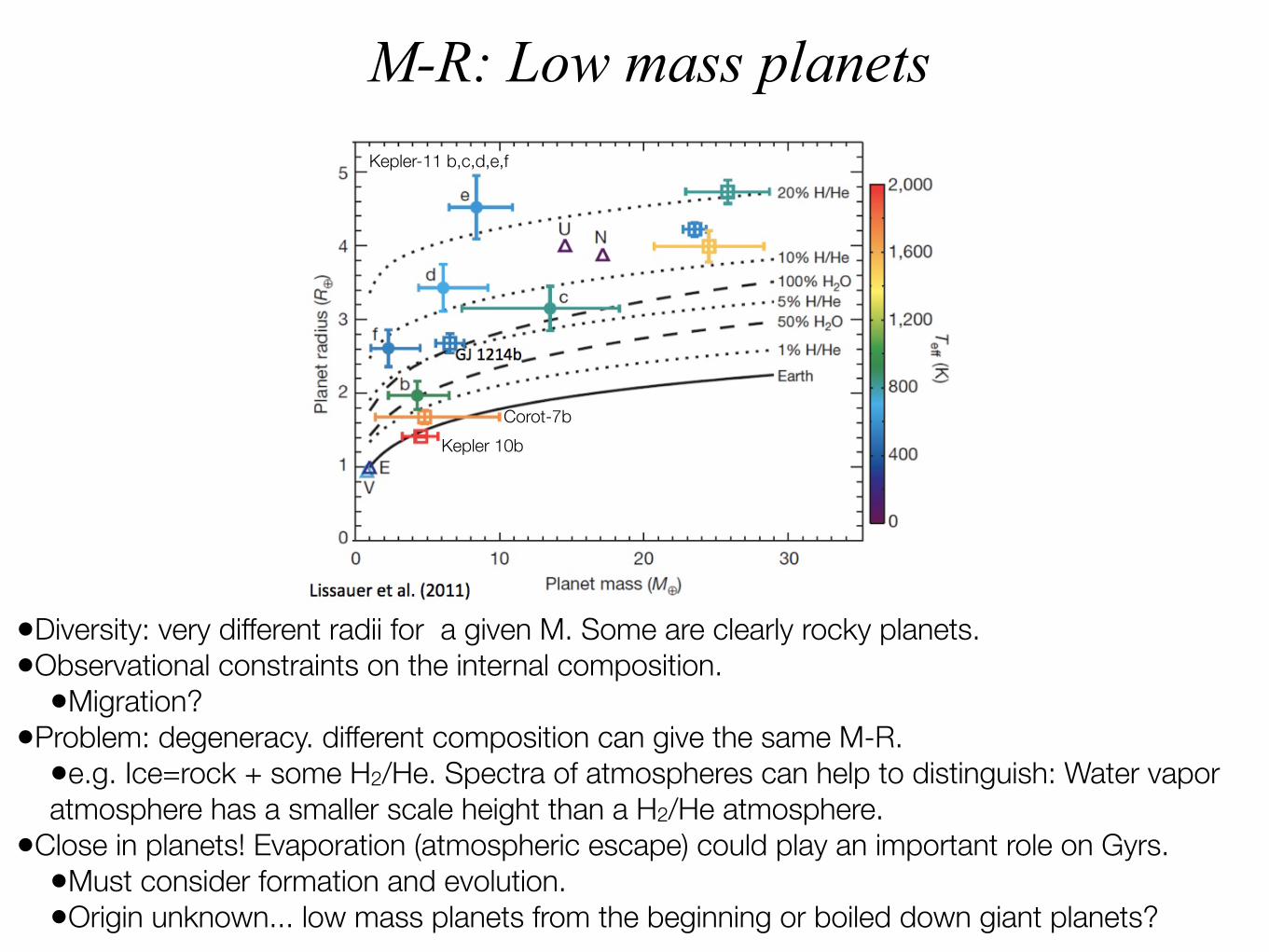
M-R: Low mass planets

Kepler 10b

Corot-7b

Kepler-11 b,c,d,e,f

•Diversity: very different radii for a given M. Some are clearly rocky planets.•Observational constraints on the internal composition.

•Migration?•Problem: degeneracy. different composition can give the same M-R.

•e.g. Ice=rock + some H2/He. Spectra of atmospheres can help to distinguish: Water vapor atmosphere has a smaller scale height than a H2/He atmosphere.

•Close in planets! Evaporation (atmospheric escape) could play an important role on Gyrs.•Must consider formation and evolution. •Origin unknown... low mass planets from the beginning or boiled down giant planets?

Additional observations

Janson et al. 2011

Direct imaging: planets form hot

•The two competing models for giant planet formation, core accretion and direct collapse, predict different initial conditions for planet evolution.•For direct collapse, planets should initially be very hot.•For core accretion, they can also be cold.

•Observations point to a “Hot start”.

•This could help to distinguish formation models.

Miller & Fortney 2010Guillot et al.

Transits: correlation planetary core mass and stellar metallicity

•Transit observations & RV mass measurements show that the core mass of giant planets, and the stellar metallicity are positively correlated.•This is reproduced by core accretion models.•Recent observations maybe even indicate that that all giant planets contain at least 10 ME of metals.•For direct collapse, planets can result both enriched and depleted.

Questions?