NBER WORKING PAPER SERIES

IS THE BUSINESS CYCLE ANECESSARY CONSEQUENCE CE

STOCHASTIC GROWTH?

Julio J. RotembergMichael Woodford

Working Paper No. 4650

NATIONAL BUREAU OF ECONOMIC RESEARCH1050 Massachusetts Avenue

Cambridge, MA 02138Febniazy 1994

We wish to thank Ludwig Chincarini for research assistance, John Cochrane, John HuizingzLucrezia Reichlin, and Argia Sbordone for helpful discussions, and the NSF for researchsupport. This paper is part of NBER's research program in Economic Fluctuations. Anyopinions expressed are those of the authors and not those of the National Bureau of EconomicResearch.

NBER Working Paper #4650February 1994

IS THE BUSINESS CYCLE ANECESSARY CONSEQUENCE OF

STOCHASTIC GROWTH?

ABSTRACT

We compute the forecastable changes in output, consumption, and hours implied by a

VAR that includes the growth rate of private value added, the share of output that is consumed,

and the detrended level of private hours. We show that the size of the forecastable changes in

output greatly exceeds that predicted by a standard stochastic growth model,of the kind studied

by real business cycle theorists. Contrary to the model's implications, forecastable movements

in labor productivity are small and only weakly related to forecasted changes in output. Also,

forecasted movements in investment and hours are positively correlated with forecasted

movements in output Finally, and again in contrast to what the growth model implies, forecasted

output movements are positively related to the current level of the consumption share and

negatively related to the level of hours. We also show that these contrasts between the model

and the observations are robust to allowance for measurement error and a variety of other types

of transitory disturbances.

Julio J. Rotemberg Michael WoodfordDepartment of Economics Department of Economics

E52A32 University of ChicagoM.I.T. 1126 E 59th StreetCambridge, MA 02139 Chicago. IL 60637and NBER and NBER

1 Introduction

The recent literature has given considerable attention to the hypothesis that fluctuations in aggregate eco-

nomic activity result fromstochastic variations in the rate of technical progr (Kydland and Prescott, 1982;

Prescott, 1986; King, Plosser and Rebelo, 1988a, 1988b; Nosier, 1989). One of the most appealing features

of this "real business cycle" (RBC) hypothesis is its parsimony - it is proposed that the same exogenous

changes in the available production technology that determine the long-run changes in output per head also

account for short-run variations in output and employment. Rather than a puzzle to be explained through

the invocation of a complex mechanism that is introduced into one's model of the economy solely for that

purpose, the business cycle is actually a necessary consequence of stochastic growth. It would be predicted

to occur even in the absence of any "frictions" not present in a standard acoclassical model of long-run

growth, and in the absence of any other disturbances to the economy, once one recognizes that the technical

progress responsible for long run growth is itself stochastic.'

The demonstration by Nelson and Plosser (1982) that U.S. real GNP has s"unit root" or stochastic trend,

rather than exhibiting only transitory fluctuations around a deterministic growth trend, greatly increased

the credence given to the real business cycle hypothesis. It is widely accepted that shocks that result in

permanent increases in the level of real GNP can only plausibly be interpreted as permanent productivity

improvements. 2 Here we wish to consider whether accepting that there is a stochastic trend in the aggregate

production technology requires one to believe also that the business cycle is largely due to (and, in essence, an

efficient response to) stochastic productivity growth. This issue has been addressed in the RBC literature

by computing the predictions of a "calibrated" stochastic growth model for the variability of output, hours

worked, and other aggregate quantities, assuming technology shocks of the size indicated by some measure

of the variability of technical progress. The question posed is whether even in the absence of other stochastic

disturbances to the economy, one would expect to see business cycles of the size and character observed.

Typically, such exercises have concluded that technology shocks alone would predict variations in output

'Thus Prtt (IS) writes, "These ('' cycleJ cbscnaloes should not be pnsIing, for they are what standard.nnn.k thc predicts. For the United Stan, In fact, ._ 'iven lbs nature of the .&sngb.g production possibility set, what

would be p,nsllng is It the p dId not display these larp Sactuations In o.etpua sad ang4oymad—"tSee, e.g.. P''d sad Flsdn (1959, S I).5We will, for purpos of the Inquiry, tilts at face value the evidence just eluded to. Thu. we will not hat question whetheran really be certain that U.S. real CNP baa a unit root, or whether steôssthc prtOJvIty growth should be regarded

as an ezogus pro to whld. lbs pattern of resource siloenalon adept, rather than an endogenous consequence ofdiangs hi the pastern of resource allocation that may be ultimately caned by shoda of another sort.

2

of roughly the magnitude observed (see, for example, Ploeser 1989). They have also concluded that these

fluctuations have the right characteristics, in the sense that the relative volatility of quantities such as

aggregate consumption and investment spending, and their degree of co-movement with output fluctuations,

correspond roughly to the predictions of the model. Thus it is argued that, granting the existence of the

stochastic technical progress and the essential correctness of the neoclassical growth model used to generate

the predicted effects of technology shocks on aggregate variables, one can conclude that technology shocks

account for a large part of the aggregate fluctuations that are observed. Moreover, it is suggested that such

additional variation in aggregate quantities as may be due to other independent disturbances makes little

difference for the overall character of business cycles.

Here we undertake a similar exercise, but using a different diagnostic for whether the model can account

for the kind of business cycles that we observe. We argue that an important feature of observed business

cycles is variation in the rate at which output can be forecasted to grow in the future. Indeed, it seems to

us that this is an essential aspect of what people mean when they refer to "business cycles" -at different

points in time (different "phases of the cycle" in the language popularized by Wesley Mitchell) the outlook

for the economy is different. Note that output growth could exhibit substantial variation even in the absence

of cycles of this sort. Output might be a random walk, so that the probability distribution over possible

future growth patterns would at all times be the same. We show in the next section that this i. not true

for aggregate fluctuations in the postwar U.S. — instead, there are significant fluctuations in the forecastable

future growth in output and other aggregate quantities. Indeed, over a horizon of two to three years, we

show that more than half of the variation in output growth is forecastable (even using only a very small set

of forecasting variables).

We then ask whether a stochastic growth model would predict fluctuations in the forecastable changes

in aggregate quantities of the kind observed. We show that, at least for a popular variant of the model

often used in the RBC literature, the answer is absolutely not. Under a standard calibration of the model

W.do not, otmw.e, daint onginality for this ohen..aloa. na Nelson sad Pleaser first directed Miatia. to the extentso which agp.gas. ostpul was similar to a random walk, and argued that this susse.ted an important role (or •aspply shocks"in the generation of observed fluctuatioss, ma aaflbon ban shown that output is net In fact a madam walk (even if It hasa uait root). The point of the sIts reported hen I. to characterize the famaataUs fluctuations na way that facilitatapsñ.on with it.. predictions of $ real busiss cycle model.s1imt model, including tha pastier calibration that we 'a., is sentisiiy identical to the model with a randomwalk in tethnolog considered by Pleaser (1%9) and bj King. Please and Rabelo (1988b) (b.aeaMr, K-P-a). The model ofaristiano and Eldbalb.uw (1993) is also quite siagar, thougjt certain of their paseter values as. rather diffesent. W. alsodiscus. below the consequonce 01 variation in the meat importana of the parameters.

3

parameters, the variability of the forecastable changes in output predicted by the model is much smaller

than that which is indicated by.a VAR model of the U.S. data. Essentially, the model predicts that output

should be much closer to a random walk than is actually the case.

This finding is related to an observation by Watson (1993). who shows that the RBC model cannot

explain the peak of the spectrum of output growth at business cycle frequencies. It is also related to the

findings of Cogley and Nason (1993), who criticise several variant aBC models on the grounds that the

models cannot account for the observed degree ci serial correlation 1 output growth. We believe that we

have identified an even greater discrepancy between the model and the data by analysing several variables

simultaneously. For one thing, as has been stressed by Cochrane and Sbordone (1988), Coclirane (1994a),

and Evans and Rtichlin (1993), estimates of the forecastability of output growth are greatly increased by

the use of a multivariate system.'

An even more important novelty in our analysis is that we identi4' three features of the co-movement

of various forecasted series that are inconsistent with our basic stochastic growth model. The first is that

predictable movements in output and predictable movements in the average product of labor bear little

relation to each other and, when they are related to each other, they axe often negatively correlated. By

contrast, the model associates predictable increases in output with capital accumulation which raises labor

productivity. Thus predictable movements in output should be strongly positively associated with predictable

movements in productivity. The second is that predictable increases in output axe correlated with predictable

increases in the labor input. By contrast, under standard calibrations, the growth model implies that the

labor input should be above its long run value when output is below its long run value, and vice versa1 so

that the two quantities are always expected to move in opposite directions. Finally, as has been pointed

out repeatedly (see e.g., CampbeU 1987, Cochraae 1994a), the data suggest that high levels of the ratio of

consumption to output are associated with increases in output (and with smaller increases in consumption).

We show that this too is inconsistent with the growth model.

We thus believe that we have identified important respects in which a simple stochastic growth model

does not predict aegate fluctuations of the kind observed. It might be argued that this is a fine point,

to be addressed by more sophisticated versions of the RBC model1 and that it does not detract from the

Ths problem that this pose for rat b cyde theory Ialso discussed in Codwsa. (flash).

4

basic model's success in accounting for the overall variability of output, investment, and so on, and for the

correlations between overall variations in these variables. However, the significance that one attaches to the

successes typically cited in the RBC literature depends upon how one proposes to separate out the "cyclical"

movements in aggregate quantities from the trend growth in those quantities (that most economists would

explai, in terms of technical progress, regardless of their view of the cycle).

One simple approach to characterization of the cyclical movements that a business cycle theory should

explain is to subtract a linear trend from (the logarithm of) each of the aggregate time series, as in King,

Plosser and Rebelo (1988a). This approach, however, does not make sense if one accepts the evidence referred

to above for the existence of a stochastic trend. An alternative approach, used by many authors following

Kydland and Prescott (1982), is to extract a complicated nonlinear trend from each aggregate time series

using the 'Hodrick-Prescott filter". ' This allows for a shifting trend, but has the disadvantage that the

shifting trend that is removed from the data (actually, the several shifting trends that are extracted from

the different aggregate series) is not modeled; the theoretical model that is used by Kydland and Prescott to

explain the cyclical variations in the data involves no trend growth at all, and so the effects of shifts in the

trend on the variables' deviations from trend are not modeled. This not only casts doubt upon the reliability

of the authors' numerical results; it undermines a principal intellectual appeal of the RBC approach, namely,

the prospect of an integrated theory of growth and the cycle.

Authors such as K-P-ft and Christiano and Lichenbaum (1992) avoid this dilemma by assuming a random

walk in productivity. In this case, the model predicts the existence of a stochastic trend in real activity, and

indeed the technology shocks that are to explain short-run fluctuations are nothing other than the shifts

in this stochastic trend. There remains, however, the question of how to define "cycliS" variations in the

presence of a stochastic trend. These authors (and likewise Nasser (1989)) simply discuss the unconditional

moments of the growth rates of aggregate quantities such as output and investment, on the ground that

both according to the theoretical model and in the U.S. data, the aggregate quantities are non-stationary

while their growth rates are stationary (and so have well-defined momenta). But it is not obvious that the

features of the aggregate data that are emphasised in this way should be taken to characterize the business

cycle. Probably the most widely accepted proposal for defining a ecycicala component of time series of this

7For di.c,,ssion .1 the propenia of this 6h .nd p.thon .11k other radhods ddetrmdlng, as Kin4 and Rcbao (1903).

5

kind is that of Beveridge and Nelson (1981), namely, to define the "trend" component of &random variable

{X} at date t S'

X't'd limE4X,4r—Tlogyx) (1)

where the constant lx is the unconditional expected rate of growth of X. The "cyclical" component is then

X7c

= limE4Xg—X,+r+Tlogixl

But in this case, the cyclical component is exactly the (orecastable change in the variable, over an infinite

horizon. Identification of the degree of cyclical variation in various aggregate quantities, and of the co-

movements in these cyclical variations, then amounts to the analysis of the forecnstahle changes in those

variables. The only difference in our approach is that we also consider forecastable changes over shorter

horizons, and in fact we give greatest emphasis to the forecastahle changes over a two- to three-year horizon.

One reason for this is that we find evidence in the U.S. data for a particularly high degree of forecastability

of output growth over this horizon, and it seems natural to us to identify exactly this phenomenon as "the

business cycle". If one does so, however, one must conclude that the stochastic growth model cannot account

at all for either the existence or nature of the cycle.

Of course, a more complex aBC model might do better at explaining the cycle in this sense. In particular,

the assumption of a significant forecastable component to productivity growth (instead of a random walk)

ought to result in a prediction of much more forecastable output growth as well. We discuss some simple

alternative models of technical progress in section 6 below, but do not intend to consider this problem in

any generality. Instead, our main point is that a model with stochastic growth need not possess abusiness

cycle to any significant extent, and insofar as one does, the features of the model that account for the cycle

will be largely independent of those that account for the stochastic trend. this point remains valid whether

the cycle is ultimately due to transitory exogenous shocks to productivity, or to shocks of some other kind.

Thus the mere fact that stochastic productivity growth can be inferred from the presence of a stochastic

trend in output does not, in itself provide support for the real business cycle hypothesis as to the source of

the cycle.

'Here we wu thM {Xi} I .tasiasaz.

6

In section I we document the fbrecastable changes in output and other aggregate quantities for the

postwar US., using a simple vector autoregression (VAR) framework. In addition to showing the importance

of these forecastable changes, we show that a definition of "the business cycle" in terms of variations in

forecasted private output growth coincides empirically with other familiar definitions; for example, we show

that our dating of cycles on these grounds would be similar to the NBER's, or to what one would obtain

from a simple linear detrending of (the logarithm 01) private output. In section 2, we review the predictions

of a simple stochastic growth model (the real business cycle model of K-P-R) regarding forecastable changes

in aggregate quantities. In section 3, we present the numerical predictions from a calibrated version of the

model (intended to match the US. economy) and compare them to our empirical results. Section 4 considers

the effect of varying the preference parameters of the model. We show that this can help the model explain

certain features of the forecastable components of output, consumption and hours but only at the expense

of more counterfactuai implications concerning the unforecastable movements in these variables. Section 5

shows that our conclusions are robust both with respect to transitory measurement error in various series

and to the presence of certain other types of transitory disturbances. Section 6 briefly considers alternative

stochastic processes for technology, and Section 7 concludes.

2 Forecastable Movements in Output, Consumption and Hours

In this section we describe the statistical properties of aggregate US. output, consumption, and hours,

with particular attention to the existence of a "business cycle" in the sense of forecantable changes in these

variables. We use a three-variable VAR to characterize these forecastable movements.

Our results obviously depend upon the VAR specification used, and so we discuss our reasons for particular

interest in the system that we estimate. First of all, we wish to compare the properties of the U.S. data

to the predictions of a standard stochastic growth model. This requires that we use series that represent

empirical correlates of variables that are determined in that model. The aBC literature has stressed its

predictions for the movements in aggregate output, consumption, and hours. Moreover, the estimation of

a joint stochastic process for these variables also implies processes foe labor productivity (output per hour)

arid investment (output that is not consumed). Thus, we are in fact estimating the joint behavior of all of

the variables with which the model is concerned.

7

We do not include in our forecasting regressions certain variables, such as interest-rate spreads, that have

been argued by Friedman and Kuttner (1992) and others to be useful in forecasting output. The reason

is that the co-movement of these variables with output is not modeled in the standard growth model. Of

course, it might be considered a detect of the model that it does not explain relationships of that kind, if

they are in fact found useful in forecasting. But here we wish to consider the extent to which an ItBC model

correctly explains the co-movements of the variables that it clearly aime to explain. Mao, the variables that

we study here are ones that must be modeled in any business cycle theory, so that our characterization of

the data should prove useful in theevaluation of a wide range of potential theories.

Secondly, we wish to avoid the contrasting pitfalls of underestimating the forecastabiity of aggregate

fluctuations due to omission of useful forecasting variables on the one hand, and of overestimating their

forecastability due to insufficient degrees of freedom on the other. To avoid overfitting, we use a small VAR

with only a few lags. On the other hand, the few variables used are ones that are expected to be useful in

the identification of forecastable output growth. Because we are interested in forecastable output growth,

output growth itself must be one of the variables in our system.

It follows from simple "permanent income hypothesis" considerations that the consumption share in

output should forecast future output growth, and the usefulness of the consumption share as a forecasting

variable has been verified by Campbell (1987), Cochrane and Sbordone (1988), Cochrane (1994a), and King,

Plosger, Stock and Watson (1991) [hereafter, IC-P-S-W]. Likewise, the idea that variations in the labor input

can be used to predict future changes in output has been used to identify temporary output fluctuations

in a VAR framework by Blanchard aadQuah (1989) and Evans (1989). Furthermore, as we explain in

the next section, the stochastic growth model implies that expected growth is a function of a certain state

variable (the aggregate capital stock deflated by the labor force and the state of technology). According to

that model, both the consumption-output ratio and hours relative to the labor force should also be functions

of that state variable, and hence either variable should supply .11 of the information that is relevant for

forecasting future output growth.

We still face a choice between several possible measures of output, consumption and bouts. One issue

'Thss .athon we the unanpIoS raze, niber than heun, — thà meanire of variations in th, labor input. For citpupa hours .rc nfesbls. bora,we of lbS elsa Males to lbs labor input with width the RBC model I concerned.Beanie detrended P"' bows a,. stationary. — disoi..ed bela, they can save — a cyclical Indicator In a way similar tothe unemployment rate.

8

is how to deal with hours and output purchased by the government, given that versions of the model used

in the RBC literature generally ignore government altogether. We have chosen to interpret the staadath

model as a model of fluctuations in private output sad hours; we explain in the next section how such an

interpretation is possible even when the government don bin some hours and purchase some of private

output. ID As a consequence, our output measure is real private value added, and our hours measure is

hours worked in the private sector.

Another issue is the choice of a measure of consumption. Because the consumption decision modeled in

the standard growth model is demand for a non-durable consumption good, we use consumer expenditure

on non-durable. and services as our measure of consumption. This is also the consumption measure that

one has the most reason to expect to forecast future output on permanent-income grounds, and it is the

one used in the studies of output rorecastability mentioned above. This choice has the consequence that we

identify consumer durable. purchases as part of "investment" in the growth model.

A further issue is how to deal with growth of the labor force (also typically ignored in the literature). In

the next section, we construct a model with deterministic growth in the available labor force and show that

it implies that hour. must be trend stationary. This implication is borne out by the data. The last column

of Table 1 reports a rejection, using a Dicicey-Fuller test, of the hypothesis that private hours have a unit

root once one allows for a deterministic trend. IS-

The time series that we use, then, are the logarithms of private output, consumption of nondurables

'°By this we do not mean to assert that we present a model in which government purchases have no effect upon tbsdetem,iasaion of private awegasn our model sen- that useinmens purchases, while non-trivial in sire, are non-stochastic.While this specification would obviously he contradicted by the data on ovemment purchases, we cannot model them insmore realistic ny without considering a maw pIa. model — in paiticuler, a model with multiple stochastic distrnban tothe economy. A similar caveat applies to our tr of pepulation 1rowth.

"We measure real pavss. value added, or privale output", — the dulferece between real CNP sad 5overemcz,t sectorvalue-added, both measured In 3982 dollars,

t3Our m.,n it Sprint, hours" S total man-Lou,. repes-ted by non-agriadtursi establishments, minus man-hours employedby the ovaan.. We an thus implicitly assuming that changes in .gri.cnjturai bows an proportional to cheng is, privatenon-apicuitural hones. Because our aol. metes, below I. with variations in the logarithm of privat, how., the multiplicationof our measlu, by & constant factor grater than one, to reflect the pseca of agricultursl hours, would not ailed any of ourr,dts.

t3flapj,o sad Watson (1988) show, by contrast, that one cannot reject the hypothesis that total hour. areben one dow not control t a deterministic umel. Give, the growth In both population and in labor torce participation,

their finding in not narpeiaiug. IC-P-It show instead that pa capita beige ar, stationary. We do not use per capita hours firtwo reasons, The fins is thea pa capita horn, have taUght desaminisaic trend it their own which Is probably due to varyingparticipation rata that is, if one allows for a trawl Ii, an autoregression of pa capita horns, one can reject the hypotbmia ofa raw coSEde,s on the trend (even though the sales passes ae tat. of etationarity, and the estimated tread growth rate isemail). Second, the use of pa capita variables would require, Ia consistency, that population growth enter as a state variable ofour theoretical model. In this case, stochastic variations in population growth would hecome $ semed sousa of disturbances tothe model, in addition to stochastic technical progs. This conclusion would be avoided only if we. to assume detenniniaticpopulation growth, 'a, which caee the use of detrended hours sad par capita hours would be equally appropriate.

9

and services, and detrended privite hours. Because we use lower case letters to denote the logarithm of

the respective upper case letter,, these variables are denoted by jig, c, and A1 respectively. ' As K-P-ft

emphasize, a standard growth model with a random walk in technology implies that vi and c1 should be

difference-stationary, and these two variables should be co-integrated, since c1 — yj is predicted to be a

stationary variable. Table I show, that our data are consistent with these predictions as well. One can

reject the hypothesis that the consumption share and the rate of growth of private output have unit roots

at the 1% significance level. The difterence-etationarity of consumption and output, and the stationarity of

the consumption-output ratio, are also reported in K-P-S-W, where the issue is discussed in more detail.

Hence our VAR specification is

= Ax...1 + eg (2)

whereCl

(c1—y€)A1 4= and =

(c,_i — ps—I) (I

0

and only the first three TOWS of A need to be estimated. This autoregression includes only two lags. One

reason for ignoring further lags is that, when we included them, these were generally not statistically signif-

icantly different from zero. 25 A second reason is that we want to avoid overfitting our VAR. Overfitting

is a particular concern in that it could lead us to overstate the extent to which aggregate variables are

forecsstable, and thus, the extent to which they are subject to cyclical movements. Thble 1 also presents

the estimates from our VAR. As can be seen from the Table, most parameters are statistically different from

zero.

We now turn to the characterization of aggregate fluctuations that can be obtained from the joint stochas-

tic process for these three time series. In Thble 2, we present the estimated values for several unconditional

second moments of the data, of the kind that have been emphasized in the aBC literature. We focus on

the behavior of private output Us, consumption c4, investment i5, detrended private hours A51 and--labor

"We rae.. the notation L, f print. bow., p.1w to dearndlng.'5Note that a VAR of ibis sest I equiwiast, expt In the way that lap are tnmcated, to an error-correction model of the

kind etimatsd by K.P.S.W .nd by Codirane (1994., 199th).Addifl dibor just a third or both a third and a fourth lag of all ,ariable. kath to just two aseifidait. that are atatlatically

.ignificaS at the 5% lsnb the third kg of detra.ded he,g, I. $ .ipifiaat -Wa—-'— of both the 1rowth In o,stpui and of theconsumption share.

to

productivity p.. We have discussed above the measures that we use for output, consumption and hours; the

other two series are constructed from these, to ensure that our data satisfy the accounting identities linking

these quantities in the theoretical model. Thus we construct a series for the growth rate of investment using

only our data on the growth in output and consumption, using the relation

scAt, + (1— sc)aig = ày.

In the nat section we derive this accounting relation for our theoretical model, from explicit assumptions

about government behavior. To compute Al using this formula, we need to know sc. The ratio sc/(1—sc) is

the average ratio of consumption to investment spending. Using postwar U.S. data, and letting consumption

be equal to consumer expenditure of nondurables and services while investment equals the turn of gross fixed

investment and consumer spending on durables, we obtain an scequal to 0.70. We similarly construct our

series for growth in labor productivity from our series for growth of output and hours, using the relation

Ap, = ày, — Ah

(This follows, up to a constant, from the standard definition of average labor productivity.) The first column

of Table 2 presents the unconditional standard deviations of the (stationary) growth rate of private output,

the ratio, of the unconditional standard deviations of the growth rates of each of the other aggregates just

mentioned to the standard deviation of output growth, and a number of unconditional correlations among

these series. As is emphasized in the RBC literature, investment growth ismore volatile than output growth

while consumption growth is less so; productivity growth exhibits considerable variability; and the growth

rates of consumption, investment, hours and productivity are all strongly positively correlated with growth

in output. (The second column presents the theoretical predictions of the calibrated stochastic growth model

discussed in the next section.)

We next compute the expected changes in each of these aggregates implied by our VAR model. We

denote the difference between the expected value at time I of Vt+k and the current value of y, by £4'. This

is givea by

(3)

where e, is a vector that has a one in the first position and zeros in all others. For the case where k =oo,

'I

we have (minus) the Beveridge-Nelson definition of the cyclical component of log Y1, which is given by

£ =e(I—A)1AZ

The expected percent change in consumption, is similarly given by

(4)

where e is a vector whose second element equals one while the others equal zero and the second equality

defines B. The expected percent change in hours is given by

(5)

where eg is defined analogously to e1 and c2 while the second equality defines Bt. The expected percentage

changes in investment and in productivity are then computed as linear combinations of these.

Letting V denote the variance-covariance matrix of 2, the variance ofLit is

(6)

and similarly for the variances of the expected changes in each of the other aggregates. The standard

deviations for these expected changes are presented in Table 3. This table also presents a measure of

uncertainty for these standard errors. This measure of uncertainty is the standard deviation of the estimate

based on the uncertainty concerning the elements of A. "

The table shows that the standard error of the expected changes for output grows as the horizon Lengthens

from one to twelve quarters. The largest predictable movements occur in the next twelve quarters and the

standard deviation of these predictable movements is above 32%. This number can be compared tothat in

the next to last column, which gives the standard deviation of the unpredictable movements in output over

the same horizon. This standard deviation equals only 3.0%. Thus the size of the predictablemovements

over the next three years exceeds the size of the unpredictable movements. This fact is reflected in the

last column, which gives the ratio of the variance of the expected changes over the total variance of output

changes. This measure of iV is even slightly higher (equal to .55) at the 8 quarter horizon, due to the Lower

variance of the unpredictable movements at the shorter horizon.

'TWe cainp'ifled the vector of derIvative. D ofsadi standard deviation with respect to cbs slosass of A. The verisnes at

ow estimate is then D'OD where 0 is the vanana.conñanoe wa4riz at the denenta of A.

12

For horizons larger than 12 quarters, both the It' and, more surprisingly, the size of expected output

changes falls. However, the declines in the size of this predictable components are very small and, indeed, are

not statistically different from zero given the uncertaintyabout the parameters of A. ' On the other hand,

the difference between the predictability of output growth at short horizons and the predictability of output

growth over the next two to three years is both substantial and statistically significant. The high frequency

movements in output are largely unpredictable: less than a third of the variance of output i, predictable

over the nat quarter. By contrast, output movements over two to three years are dominated by predictable

'cyclical" components which are our main focus of attention in this paper.

Since the size of these predictable movements is largest at the 12 quarter horizon, we focus mostly on this

horizon. (We also prefer this to a longer horizon because the predictable movements over a shorter horizon

can be estimated with greater precision.) However, it is important to realize that the expected movements

in output over the next eight, twelve or infinite quarters are very similar to each other. To see this, Figure

1 graphs the demeaned expected declines in output over these three horizons using the same scale. We

show expected declines, as opposed to expected increases, because recessions ought tobe associated with

expected increases in output and we wish to represent these as low values for our cyclical indicator. In this

Figure we have also indicated the troughs of recessions as determined by the NBER. We see that output is

expected to grow fast at these NBER troughs so that expected output dedlineshave some similarity with this

particular business cycle indicator. " It is worth noting, however, that our cyclical indicator tends to reach

its lowest value one quarter alter the NBER troughs. The reason may be that the NBER uses subsequent

information to construct its chronolop of troughs. Thus the end of the recession is defined to occur just

before output grows more than it was expected to. This positive innovation in output cannot be predicted

with our method. On the other hand, this positive innovation tends to raise predicted output growth since

lagged output growth predicts future output growth to some extent.

In Figure 2, we superimpose our measure of expected declines over the next twelve quarters with linearly

detrended values of our output measure itselt The Figure shows that our cyclical indicator is very closely

associated with detrended private value added. There are sows interesting differences, however. First, as

"This. po..IW. intapresasioa dsiw fin&np would be thai output I expected to have essensisily completed the sdlustmcidto iii long.run nit,. within & period o( two to three years, afl which Utile farther change in output can be forecasted.

tTh.ou. cas, where the indicates. differ is In the ca,,d the last recession. As would be suggested by oter series, the recoveryfrom this "tro,i&C initially weak.

13

with the NRER troughs, detrended output appears to lead slightly our business cycle indicator. Once again,

this may be due to the fact that unpredictable upturns in activity are responsible for the turning points of

the detrended output series. 20 -

The two lines also differ in someof their low frequency aspects. First, our predicted output growth series

is relatively smaller in the 1960's than the deviation from a linear trend. While the linear detrending method

attributes all the unusually large growth in the 1960'. to an abnormally large cyclical expansion, our method

attributes some of it to variables that affect steady state output. By the same token, linearly detrended

output falls more in the 1970's than our series. Finally, in the 1980'. linearly detrended output remains low

in part because the high growth of the 1960's did not persist. By contrast, our series treats the Reagan

expansion as unusually large.

In addition to forecastable output movements, we find some forecastable consumption movements as well.

3t As Table 3 shows, the volatility of expected consumption growth is substantially smaller than the volatility

of expected output growth. This is not very surprising given that the volatility of overall consumption growth

is smaller than the volatility of output growth. What is notable about the behavior of consumption is that

the relative variability of consumption is particularly small at short horizons. Expected consumption changes

are less than half as large as output changes at horizons of under one year. As the horizon lengthens, the

standard deviation of expected consumption changes keeps growing while thnt of output does not. The

result is that the standard deviation of the difference between expected long run consumption and current

consumption is about 88% as large as the corresponding standard deviation for output. Table 3 also shows

that expected investment growth i. more volatile than expected growth in output. This is not surprising

given that expected growth in consumption is less volatile than expected growth in output. The magnitude

of the expected changes in hours worked reported in Table 3 is very similar to that ofexpected changes in

output. This may seem surprising given that K-P-ft report that the standard deviation or the growth in

hours is only 80% as large as the standard deviation of the growth in output. Finally, Table 3 reports the

20Wom a puaeiy mechanical point of view the fluding that our Indicator lag. behind output Is not eurpritlog duct ciiilndiata Is heavily Influenced by hour. nbd, which as. known to lag behind aggcgM. activity. This raises the questionof whether our cycLe-al Indicator woi,W have been different fe had allowed detre,ded output to influenos It. To ditch thiswe r.a a res4oa esp'"1"g output powtb with our wujable and, In aMities, oct lag of detsunded output. The coefficiei,ton detranded output was .tati.tically Insignificant and the other codtda,t timata did not change. Th' hours, the ratio of

conatsnptloa to output, and the rat, of poweb of output tahn more Information about future output gowth."The enatance of such mo,et. — aviolation do .imple version of the rational.expectations permanent .nts bypotla'a

- baa bee demonstrated before (e.g., Campbell and Mankiw, 1089).

14

volatility of expected changes in labor productivity. At horizons above one yea:, the standard deviation of

this is len than one third of the standard deviation of expected output growth.

La Tables 4 and 5 we give further statistics that describe the behavior of cyclical output, consumption and

hours indicated by our VAR model. Table 4 ii devoted to studying which of our regressors is particularly

responsible kr forecasting output growth at various horizons. Table 5 focuses instead on the expected

co-movements of the five aggregate variables.

Table 4 gives the correlations of and the value at t of our three regressors, Ay1, (ci — yg) and h,.

The forecast of output growth in the next quarter is most higjily correlated with current output growth. By

contrast, the other two variables, especially detrended hours, are more useful for predicting output growth

over longer horizons. Thus hours prove to be an important indicator of the current state of the business

cycle.

Table 5 presents regression coefficients of the expected changes mc, 1., p and ion expected changes in y.

These coefficients indicate the percentage by which a given variable caa be expected to change if one know.

that output is expected to increase by one patent. The covariance between expected consumption growth

over the next k quarters and expected output growth over this same interval ii given by .a'va:. Thus, the

regression coefficient relating changes in c at horizon k to the changes in j over the same period is given by

7a:'vB:

The other coefficients can be computed analogously.

Table 5 indicates that the elasticity of expected consumption growth with respect to expected output

growth equais about one-fourth for a one quarter horizon. It grows with the horizon so that it exceed.

one-half for the infinite horizon. Given that the standard deviation of consumption changes is smaller than

that (or output, it is not surprising that consumption does not respond one for one to expected changes in

output. While expected consumption growth is not very elastic with respect to expected output growth,

investment growth is, and this is consistent with the large volatility of investment changes.

Expected hours growth responds nearly one for one to expected changes in output. As a result, expected

productivity is largely unrelated to expected changes in output. This lack of correlation may be surprising

given that output growth is generally positively correlated with productivity growth. The table indicates

15

that this correlation is due mainly to unexpected changes in either output or productivity. The data are

thus consistent with the idea that measured productivity growth is strongly associated with current shocks.

The regression coefficients in Table 5 can be used together with the standard deviations reported in Thble

3 to compute correlations between expected changes in consumption and hours on the one band and expected

changes in income on the other. Particularly for horizons above 8 quarters the regression coefficients of both

consumption and hours are close to the ratio of their respective standard deviation. to that ci expected

output growth. If they were equal, Lit and Act (or Lit and Ah5) would be perfectly correlated. As it is,

the correlation between expected changes is high but not equal to one. The correlation between expected

consumption growth over the next 8 quarters and expected output growth is .79 while that between expected

hour. growth and expected output growth is O.9T. The high values of these correlations suggest that there

is a single underlying state variable that determines the position of the economy in the business cycle and

hence the evolution of expected output, consumption and hours.

In the stochastic growth model that we consider in the next section, there is a state variable of this sort.

As we show, this state variable is the ratio of the current capital stock to the capital stock that is expected

to exist in the infinite future. The question then becomes whether this state variable can explain the size

and nature of the movements and co-movements documented in this section.

3 A Simple Stochastic Growth Model

In this section we describe the structure of a stochastic growth model, the predictions of which we wish to

compare with the properties of the aggregate time series just discussed. The model extends the stochastic

growth model of Broth and Mirman (1972) to allow for a labor-leisure choke; it is essentially identical to the

model analyzed in K-P-K and in Plosser (1989). We consider this variant, rather than familiar alternatives

such as the models analyzed in Prescott (1986), because it implies a stochastic trend of the kind assumed

in our treatment of the data. The primary innovations in our own presentation of the model are explicit

treatment of government purchases and labor force growth, in order to tighten the relation between the

theoretical model and our time series."Tb. pndidla.s of the model that we ps.e. e an n fast almost 'l to those of the K-P.R model. We csnt4.. e.g

t.-t of the govunmest so that ow nodjs jndidios.s regarding the e,oludM of (pe4sas) capital, hours, amsumptloa,and output an ida,sical to thcse of a modeL with so s.anat.

16

Consider an economy made up of a fixed number of identical infinite-lived households. We will suppose

that there is growth over time in an exogenous state variable N, that we refer to as the size of the labor

force, but that in our model simply represents a change in the preferences of the representative household.

(Each household may be supposed to be made up of many individuals whose number may grow with time.)

The representative household seeks to maximize the expected value of lifetime utility

u=zof a'5(c1.ç)where fi is a constant discount factor, C, again denotes consumption by the members of the household in

period t, and LI°' denotes per total hours worked by the members of the household in period t. We let

14°t/N, be total hours worked as a ratio to the available labor lbrce. The single-period utility

(unction 4C, H) is concave, increasing in C, and decreasing in H.

In order to ensure the existence of a stationary equilibrium (in terms of suitably rescaled state variables)

despite the presence of a non-stationary technology process (specified below), we need further homogeneity

assumptions on the form of this function. The marginal utility of income A, for the representative household

each period must be given by

= uc(C,.11") (8)

flirthermore, household optimization requires that each period the marginal rate of substitution between C

and Lice must equal the real wage W, so that

Er niceua ' — WU 9I I

Equations (8) and (9) then implicitly defini Frisch labor supply and consumption demand functions

JP°'(W,N,,A,) and C(WINI,AI), which provide a useful characterization of intra-temporal preferences. 24

Our additional homogeneity assumption can then be stated as follows. There exists a parameter a> 0

such that the Frisch labor supply is homogeneous degree zero in (WN,)rtt'), and the Frisch consumption

demand is homogeneous of degree one in the same arguments. n The consequence of thu assumption is

Our Isbor Iv. yniahls Is a sal. factor for .g.gat. Isb nipply, with as'——j ccnn.ctloa —uk lb. labor f.imean. In the SL.S surveys, that mewnn only thai InthvMuais who ether ban a Job or who ass actively aechinj one, anddoes not w.11ba them according to the amount of tim. that they wish to woá.

as.., ..g., Rosenberg tad Wo.dford (1992, 1994) for fortbc disaissica of PbMth labor supply and consuniplion

m. family of utility t'mction. will, this property I - jrtbor in King, Ploc and Rebclo (1988.) and In kotenb.sgd Woodlc.d (1992).

17

that a permanent increase in the real wage leaves hours worked unchanged while desired consumption rises

proportionally. An increase in N has the saint effects as an increase in w since it increases the payment that

the household receives per unit of N'°'. Thus an increase in the labor force also lacks any effect on the value

of ff10, while C and L'°4 grow in proportion to the increase in N. Note that the case analyzed in much of

the R.BC literiture.

u(C,Jf) = c— v(Jt),

for t4H) an increasing convex function, satisfies our homogeneity assumption with a = 1.

We assume a constant rate of growth of the labor force N, so that our model has only a single source of

stochastic variation in the endogenous variables. Thus N, = Not5q for some positive constants N0 and 7N

Private output is produced by competitive flrn using a technology

= F(Kg,z,L.)

where Y, denotes private output as before, K, the private capital stock, L is private hours, and £an

exogenous technology factor, all in period 1. Stochastic variations in the technology factor are the source of

aggregate fluctuations. We introduce a stochastic trend in output, consumption, and so on (as was argued

to exist in the U.S. data) by assuming that the technology factor is • random walk with drift, i.e., that

logz,=log,+logr,_t+c. (1G)

where y, is a positive constant and {c,} is a mean-zero i.i.d. random variable.

Both factors of production are hired in competitive spot markets each period. 'The evolution of the

private capital stock is given by

= 1,+(1—S)K,

white I denotes private investment and the depredation rate 5 is a positive constant, less than or equal to

one.

The government is assumed to hire a certain constant fraction of the available labor force for its own use.

We denote this fraction by 11', it is recorded in the national income accounts as governmentvalue added.

As a result, the condition for labor market clearing i.

= 1(1+ H' (11)

18

when H, denotes private bouts per member of the labor force, or 4,/N,.

In addition, the government purchases a quantity 0, of private output in period t. We aseume that

C, = it',

where r is a positive constant, less than one. As a result, the condition for product market clearing is

C1 +1, =(1—r)F(K,,r,N,H.) (12)

Both H' and r are asumed to be constants (at some cost in realism) sothat the technology shock is the

only source of stochastic variation.

These government purchases are financed by lump-sum taxes equal to W,N,H' each period, and a

proportional tax rater on alt (actor incomes. This results in equilibrium factor demands satisfying

Fi(K,,z,N,H,) =

F2(K,,z,N,H4) =(1—r)r,

where p, denotes the alter tax rental price of capital goods in period I. These equations hold because p/(l -r)

and W,/(l — r) equal the pre-tax wage and rental rate respectively. These equilibrium conditions, along

with (12), are identical to those of a model with no government purchases in which the production (unction

F(K,zL) is replaced by (1— r)F(K,zL) and the 1usd labor supply function H'°'(W,N,,,) is replaced

by H'°'(W,N,,A,) —H'. Because neither the steady changes in N, nor the permanent changes in V/,

induced by technology have a permanent effect on H, this variable is stationary. Thus, as we suggested in

the earlier section, private hours must be trend stationary.

The equilibrium for this economy is given by the solution to a planning problem. The levels of output,

consumption and hours that solve this planning problem at any date t depend on K,, N,, the current level

of technology at I,; and on the expected evolution of technology in the future. Because; is Markovian,

the expected future evolution of technology depends only on; itself so the equilibrium at t depends only

on K,, N, and t. Moreover, it is easy to show that our preference specification implies that, output Y,

'Not. thea this does not Mnl,. say .iotssMn of the vessel psepetia of the Fthth '—'-—¼ the modi&d fandionsH(W,N,, A,) aM C(W,N,, A,)n. sim$y the wa A—...-L connpoedin to a —-l uIiflty function .4C.H + H').

19

and consumption C1 (and hence investment) are homogeneous of degree one in K1 and z5N,1 while H ii

homogeneous of degree zero in these same two variables. " This means that the rescaled levels of private

consumption, investment, output and bouts at date 1, ç. %-. , and respectively, are each functions

of just fr ,and we denote the logarithm of this state variable by x. As a result of this, the resealed level of

labor productivity P,/z s is also a function of .c4. It can be shown furthermore that Sc1 is a stationary

variable in the equilibrium, and hence that each it the resealed variables just mentioned is stationary as

well.

In a log-linear approximation to the equilibrium laws of motion, we can then write

(z — 1') =r(, — (13)

where z1 denotes the logarithm of any one of the five stationary variable, just mentioned, f is the mean

valueo(thai variable, and aC isthemeanvalueofc1. (Wewillusesubscriptsc,i,y,handpforxinrefening

subsequently to these elasticities.) The corresponding investment equation, together with the random walk

in technology, then implie. a law of motion for the state variable {cj, an approximation to which ii

(xj+t —c) = —C)—cg+i (14)

where q (I — $)r4 + 0, and 8 (1— S)/y.7g is the average fraction of the capital stock made up of

undepreciated capital from the previous period (as opposed to investment purchases during the previous

period). For the calibrated parameter values discuesed in the next section, 0< q < 1, so that (14) implies

that {cg} is indeed a stationary variable. Given an initial per-capita capital stock k0 and an initial state of

technology go, equations (13) and (14) determine the evolution of the variables {z.Kg,Cs,Ig,Ys,hi,Pi) as

a function of the sequence of technology innovations (cj.

These equations can thus be used to compute impulse response functions to a disturbance c5. As is

apparent from (14). this response simply describes the expected evolution of our variables starting from a

situation where g is away from its steady state value C. This evolution is thus identical to the deterministic

dynamics of a model with constant technology whose initial capital stock is different from its steady-state

level, Equation (13) then determines the extent to which each particular variable departs from the steady

2tSse K-P.R (a 't1 of this, .ndelse lbs la-llossr nppseelmMloa to the aq.flDziin dyu.mia used below.85Th1s problem Is saslyted in .sakn 3 of Kiag, Pleas and gaâ. (l9Ms) their notasion (or lbs elostidly .i1. tst.

20

state while (14) implies that they all converge exponentially to the steady state at the rate (1— q). The fact

that 0< q <1 indicates that the system don indeed converge. For plausible parameter values (in particular,

a plausibly low depreciation rate 4), the rate of convergence is relatively slow, so that q is near 1.

Using the baseline parameters set out in Table 6 and discussed further below, Figure 3 displays the

response of consumption, hours and output to a disturbance that raises e by one. horn an initial value of

sew, the increase in e eventually raises output and consumption by one unit while hours return to their

original value. Since the increase in £ lowers the capital stock relative to its steady state value, output is

below the new steady state as well. These parameters imply that when output is below the steady state,

consumption is even further below the steady state. This ensures that the ratio of investment to output is

above the steady state and helps raise the capital stock to its steady state value. The figure also shows that

hours are above the steady state. This occurs because the low value of the capital stock implies that wealth

is relatively low so that people reduce their consumption of leisure.

The joint stochastic process for these variable, is predicted to be such that Sy1, (ct-u,), and h, are

stationary variables, though {,p,) each poun a unit root, as is reported in section 2 for the U.S. data.

Specifically, the model predicts that

ap = r,a,c+c. (15)-

(cs—vt) = Ir..—r,4Ic (16)

14 = (17)

omitting the constants in each equation. On the other hand, both c and y, are non-stationary, as each can

be expressed as the sum of log xi (a random walk) and a stationary variable. Hence the general form of our

econometric specification in section 2 is consistent with this model.

X-P•ft describe the numerical predictions of the model regarding the variability of the growth rata of

agpegates such as per capita output, consumption, investment and hours. We wish to emphasize Stead

the character of predictable changes in such agpegates. In the case of the aggregates X1 = C,I,,Y,, or

"The modsi doe. Imply that the joint -'—1.—.L- ,.,._ M the three -.-'.—y vasisbiss should be singular. — that Isonly a .hoà esa pciod to wIdth .11 three lanciasions as. jnpatlonsl, and this Is not in,. of the VAR that -. estimateIn sectIon 2. But this Is not a predictIon of the model that .u p to ta hcxc In this partlailar respect it Is obvious that aone.ebock model Is Inadequate. It Is stIll of interes to ask to .bat .zts a partiadsr ou.shoth model predicts co.novt5of awnst. nriabla that are at all .bell., so thee. obeaved. If It do.., that mi#t be mm. hope that one she& maid beraspoasibin fw the pester part of .hat as. thsuht of as typical b.nlnae cycle?.

21

the laws of motion (13) and (14) imply that the expected growth rates are given by

Ax1 = r,4E1[icg+e — xs] + E4logr,.p — logz]

= —r541 — q1)(scs —

In writing this, it is assumed that the date * information set used in forecasting includes the state variable

s• However, since both (c,—jj) sad h are log-linear functions of this variable, it suffices that either of the

latter variables be in the information set. Since both of these variables are among our regressors in section

2, the model implies that the forecastable changes identified by our VAR specification should coincide with

the variables described above. Similarly, the laws of motion imply that

= — ICE]

= —r,(l — ,ik)(ic —

Thus the forecastable changes in all of our five variables are predicted to be perfectly collinear. l¼rthermore,

the forecastable changes in any one of the variables at different horizons are predicted to be perfectly coflinear:

for regardless of the horizon k, the torecastable change should be proportional to (x — sd.

4 Numerical Results for the Baseline Model

We now present the numerical predictions oft calibrated version of the stochastic growth model described in

the previous section, and compare them to our estimates in section 2. The calibrated parameters presented

in Thbte 6 are identical to those used by K-P-K, except that we allow for growth in the labor force. A

regression of the logarithm of private bours on a deterministic trend gives ta, the rate of growth of the labor

force. Our regression implies that this equals 1.004.

Note that preferences are specified in tenus of the coefficient a referred to in the previous section - that

can be interpreted as the reciprocal of the intertemporal elasticity of substitution of consumption holding

hours worked constant — and CUW, the elasticity of the Frisch labor supply function h'(wN,A) with respect

to the real wage. As is explained in Rotemberg sad Woodford (1992 1994), the other elasticities of the

Fitch demands can all be computed given numerical values for these two parameters, and the elasticitiesof

the Fitch demands are the only aspect of preferences that enters the log-linearized equilibriumconditions.

22

The values used in our baseline calibration — = i,gw = 4-are those that would result from a utility

function

log(Cg) + log(H - If°)

ifon average JP°' is .2 of If—H'.

The other parameter not taken directly from K-P-ft is our assumed standard deviation for the technology

shocks, e1 = .00732. This value is equal to the estimated standard deviation of innovations in the permanent

component of private output, from the VAR described in section 2. 3° According to the theoretical model

of the previous section, the trend component of log private output in the sense of (1) should exactly equal

log z1 (plus a constant), so that the variance of innovations in this variable should equal the variance of (j).

31 Thus we calibrate the variability of the innovations in technology so that the model's prediction regarding

the variability of the permanent component of private output agrees exactly with what we measure. Of

course, the fact that the model predicts variation in the permanent component does not imply anything

about variation in Ibrecastable change. in output; for example, if output were predicted to be a random

walk, there would be none. We turn next to the model's predictions regarding the size and character of the

fluctuations in the aggregate variables discussed in section 2.

First of all, the second column in Table 2 presents the predictions of the calibrated model for each of

the unconditional moments reported in that table. This is the type of test of the model emphasized by

K-p-a and by Plosaer (1989). Using this test, the model meets with a fair degree of success. This picture

of relative succ changes considerably, however, if one considers the variability of the forecastable changes

in the various aggregate variables, rather than the unconditional variability of their growth rates. Table 7

reports the predicted standard deviations of the forecastable changes A4,for each of the five variables r,

and for several different horizons k. The first thing to notice about these results is that the stochastic growth

model does not predict that there should be a great deal of variation in the forecasted change in private

30ur results are In -'-i agees with these at K-P-SW, who ropers a standard deviation of .7 for thegrowth shoth' to that three-veriahie VAR, which differs free Os,. mainly I. .iMag the share of Med Investment In paintsoutput, resha than lnt. beta. triad.. to th. labor force, — the third variable.

"It has boss cheat byLippi and RaIn (1993) that IdentIflasia. .1 .hllis In the permanent ajenponent of output using• VAR in ibis w depend. upon a se.umptioc of of the mn.ing-svaai. reçrseisasioa implied by theestimated VAR, an assumption that need not be wild In gcna1. That Is, it need s be poible to rscon the tn pama.hodc as any linear n'elJ,—'--. of the VAR Innowsions. nfl In the ceas cat, one aslal model boplia that theMA rersu.esation derived from our VAR should Indeed be "f.adama,sal'. The tine paman shoch can indeed befree the VAR residuals, for example, equations (14) and (17) imply than, should be aaaly proportional to the rSdual from•r.gnaio,, oft, on

23

output. At the 12-quarter horizon, the standard deviation of the forecastable change in output is predicted

to be .0029, whereas we estimate it to be .0326 - the model accounts for variations in forecastable output

growth of only 9% of the amplitude of the observed variations! At the infinite-horizon (the Beveridge.Nelson

cyclical component of output), the model account. for variations of only 21% of the amplitude of the observed

variations.

These results depend on assuming that the standard deviation of the technology shocks a4 is equal to

0.00732. As we explained earlier this is the standard deviation of the shock to the permanent level of

output. This standard deviation also implies that the model's overall standard deviation of output changes

is below the actual standard deviation. This can be seen by comparing the 6th column of Table 7 with the

corresponding column of Thble 3. These columns present the standard deviations of the unexpected changes

in output from one period to the next. The standard deviation of unexpected changes over one quarter

predicted by the model equals about 60% of the actual one. For the 24 quarter horizon, the model predicts

a standard deviation of unexpected changes that is much closer to the actual one.

Obviously, one could raise both the predictable and the unpredictable variability of output changes

generated by the model by raising one's estimate of o. But our value of o is not solely responsible for the

results concerning the lack of predictable output changes in the model. To see this, suppose that we set a4

so that the standard deviation of overall quarterly changes in output predicted by the model equals 0.012,

the actual standard deviation of the one quarter changes in private value added. This requires that a4 be

equal 0.0157, which is more than twice as large as our estimate. Even then, the model's predicted standard

deviation of expected output changes over eight quarters equals only 18% of the standard deviation implied

by our VAR.

Another way to see that the lack of predictable movements is not solely due to our choice of a4 is to

compare the H3'. in the last columns of the two tables. These H' 'a give the ratio of the variance of expected

changes to the total variance of changes in output and are thus independent of the level of a. The R3's

predicted by the model are much lower than the actual ones. At the 12 quarter horizon, the estimates imply

52IIe ide. lasted the fredisa of the ..ñ of the S—-' &aas that Is w.dict.d by the modal, one M& thatthe modal ac,unts (or only 1% in the Sawer case and oaly 4% In the late. 7W. Is a prdes�al. matric In certain respect.because the total vañanoe equals the sum it the nñaa Induced by Mdspedons .ho&s. Thus, If a suocesaful modal meld beSound that added other independa's disturbances to this model the other sLoths would has's to aessiat for 99% of the vaflanceof the faucastable thsns in the (01W case, and 06% in the latin.

24

that over 50% of the variance of output is predictable. By contrast, if the model were correct, only about

2% of the variance of output over this horizon would be predictable.

Another difference between the model and the data ii that the model predicts that the standard deviation

of forecasted changes in output rises whenever the horizon is lengthened. By contrast, the data suggest that

this standard deviation peaks at the 12 quarter horizon, or at any rate increases little after that horizon.

Similarly, the model predicts that the R2 should rise from the 12 to the 24 quarter horizon and this is

not true of our empirical results. Thus the forecasted fluctuations predicted by the model have a somewhat

different character than those we find in the data. The model's forecasted changes involve adjustments to the

steady state that occur over very long spans of time. Instead, the data suggest that the large (brecastable

changes occur over shorter Thusiness cycle5 frequencies. This finding is related to the demonstration by

Watson (1993) that the model is unable to replicate the fact that spectra of output growth have a great deal

of power at business cycle frequencies.

Perhaps the most counterintuitive contrast between the model and the data concerns the behavior of

the variability of consumption. As we saw, the estimated standard deviation of expected consumption

changes equals between one third and one half the corresponding standard deviation for output. By contrast,

the model predicts that the standard deviation of expected consumption changes should equal over twice

the standard deviation of output changes. This may be surprising since the RBC literature often counts

the prediction of relatively smooth consumption as one of the model's important successes. But because

technology shocks raise the marginal product of capital they raise interest rates and this promotes a reduction

in consumption relative to its steady state level. This reduction is so large in the case of our preference

parameters that the ratio of consumption to income actually falls. This means that consumption is expected

to grow more than income and thus the size of expected changes in con_suanption exceeds the size of expected

output changes. Another way of seeing this is to note that, in Figure 3, departures of output from the steady

state are associated with even bigger departures of consumption from its steady state. Thus the predictable

movements of consumption (towards its steady state) are larger.

In the case of investment, by contrast, the model is more accurate. While its underprediction of the total

variability of forecastable output movements leads it to underpredict the standard deviation of investment

movements, it correctly predicts that this standard deviation should be larger than that for output move-

25

meats. Investment is very large in the immediate aftermath of a positive technolo' shock because capital

is below the steady state. Later, investment is much smaller and, for this reason, the predictable movements

are large. In the data the ratio of the standard deviation of investment movements is to that of output

movements is actually slightly larger than the ratio predicted by the modeL This is just the flip side of the

model's relative overprediction of consumption movements.

The model generates predictable movement. in hours that are of roughly the same magnitude as the

predictable changes in output. This prediction is validated in the data. This is interesting because, as far

as the total variability is concerned, Table 2 shows (a. do K-P-K) that the model underpredicta the ratio of

the standard deviation of hours growth to that of output growth.

Unlike in the case of output movements, the model predicts labor productivity movements that are too

large, particularly for horizons longer than 24 months. This means that the ratio of the standard deviation

of productivity changes to that of output changes is much larger in the model than in the data, particularly

at long horizons. As we will emphasize below, these counterfactual predictions concerning productivity

movement. are particularly bothersome b.r.ne it wn unlikely that simple variants of the model can

account for it.

Because the model has just one state variable, ic, the expected changes in all the variables are perfectly

correlated. Moreover, since x is deterministically related to both current hours and the consumption share,

these variables are also perfectly correlated with all expected changes. Such perfect correlations are obviously

absent from our data. Nonetheless, all our estimates of expected changes are highly correlated with each other

and, at least for long horizons, they are also highly correlated with initial hours and the initial consumption

share. This suggests that a model with a single state variable can in principle explain a large fraction of the

cyclical movements in our variables.

While these correlations are high in our data, their sign is often not that predicted by our model. It is

apparent from Figure 3 that our parameters imply that when output is below the steady state (and rising),

hours ate above the steady state while the consumption share ii below the steady state. This means that

expected future output growth should be positively associated with the current level of hours and negatively

associated with the consumption share. Empirically, both these correlations have the opposite sign from

Notc that this laster t..,,lL...*L.., I. the opposite of what S hspU.d by the simple pemanet lucerne boU.eiis.

26

that predicted by our model. in the data, a high consumption share and a low level of hours both predict

high future growth in output.

Similar difficulties arise when we analyse the sign of the correlations between the expected changes in

our variables. These can be seen in ThbIe B which report. the regression coefficients of expected changes in

various variables on expected output growth. We do not report different coefficients for different horizons

because the model predicts that these coefficients are independent of the horizon in question. If the model

were literally correct these regressions would have no error but this is not our main concern here. Rather

we are most interested in the form of the predicted co-movement.

Our model predicts that expected consumption growth is positive when expected output growth is pos-

itive. Therefore, the regression coefficient of expected consumption growth on expected output growth is

positive. Our earlier discussion suggests the model predicts that this coefficient is well above 2. By contrast,

it is less than .5 in the data. The problem is once again that the model predicts that consumption will rise

faster than income alter a positive technology shock.

By the same token, the model implies that expected changes in investment are very negatively related to

expected increases in output. The corresponding regression coefficient is about -1.7. Investment is highest

immediately after a positive technology shock. After that, investment is expected to fall while output is

expected to rise. By contrast, our estimated regression coefficient is above 2, and implies that expected

investment growth is positively related to expected output growth.

With our parameters, our model predicts that the regression coefficient of expected hours growth on

expected output growth is negative. The reason is that a positive technology shock leads to an immediate

increase in hours. As is clear in Figure 3, hours are then expected to tall even though output rises as a

result of capital accumulation. In the data, expected output growth is positively associated with expected

hours growth. This is simply the flip side of the observation that a low level of hours is associated with an

expected increase in output in the data while it is associated with a decline in the model.

A somewhat different contrast is provided by the regression coefficient of expected labor productivity

growth on expected output growth. The model predicts this to be positive and larger than one. This is not

surprising since output is expected to rise when hours are expected to fall. The extra output is expected

to be produced by increased capital. By contrast our estimates indicate that expected productivity growth

27

S nearly unrelated to expected output growth. While the standard errors are large relative to the point

estimates, many of the coefficients in the last column of Thble 5 are negative suggesting that productivity

should fall when output rwes.

5 Alternative Preference Specifications

One obvious question that arises at this point is whether these discrepancies can be resolved by changing the

preference parameters in plwzsible ways. To shed some light on this question, we have investigated whether

changes in o'and qiw could reverie the sign of some of the predicted correlations in ways that would make

them more consistent with the data. The results are presented in Thble 9. This table presents the standard

deviation of output changes forecasted to occur in the next 12 quarters in the third column. The fourth and

111th columns present the correlation of output changes with the initial level of (C/Y) and I. respectively.

Finally, the last three columns report the regression coefficients of expected consumption growth1 expected

hours growth and expected productivity growth on expected output growth.

it is apparent from this table that, keeping a equal to 1, varying (11W does not make the model more

successful. As is well known, raising the elasticity of labor supply, raise the immediate increase in hours in

response to a positive technology shock. This means that hours are expected to decline further after such

a shock. The result is that the regression coefficient of expected hours changes on expected output changes

becomes even more negative. Moreover, the volatility of expected output falls because the increase in output

due to capital accumulation is now offset by a bigger decline in hours worked. Thus raising the elasticity of

labor supply, which has been demonstrated to help the model explain the unconditional volatility of hours

makes the predictions concerning the expected changes in hours more counterfactual.

It is possible to make some of the model's predictions more consistent with our facts by changing a.

Consider first the effect of lowering a so that utility is more nearly linear in consumption. This has the

effect of making consumption rise less in response to a technology shock so that C/V falls by more. The fall

in consumption also tends to raise labor supply so that hours rise by more. U, one assumes also that HW

is large, then hours can rise so much that output initially overshoots its long run level. This possibility is

3Tha psrtmfles of the modsi dill.from lbs others In th.s they cannot he Idatified Inn obeantion ci lbs long nan

averages of ststnnay vasisbies sicas, as opposed to usIng evidence on the dasracter ci aggregate fluctuations to — themdown. The parameter sw in particular is quite controversial tim within the RBC literature, sad lbs coasequenme of

.._.E: aIt.eniati,e values fer It as. often considered. See, e.g., Prescott (1986) sad King, floss. and Rsbeic (1988.).

28

illustrated in Figure 4 which shows impulse responses fore equal to 0.6 and IfW e(lUal to 10.

Because output overshoots its long run level, output and hours are expected to decline together. This

expected decline in output is associated with a low initial level of (dY) and a high initial level of how..

Thus the model now fits the sign of these correlations as well as the positive co-movement of expected

hours and expected output. Another possible advantage of these parameters is that they imply that labor

productivity moves in the opposite direction as output. The reason is that the output declines that follow a

positive technology shock are accompanied by capital accumulation and labor decumulation, both of which

raise labor productivity. The problem, however, is that, because both factor movements are causing labor

productivity to rise, the predicted relationship is too strong productivity is expected to fall by more than

4% for each 1% increase in output.

There is another problem with this specification of preferences. Because consumption is expected to grow

after a technology shock, its growth occurs when output is expected to decline (the regression coefficient

of expected consumption growth on expected output growth equals -5.3). While the precise magnitude of

this coefficient depends on the parameters employed, it should be clear that the fact that consumption and

output move in opposite directions is an immediate consequence of making a so low that output overshoots

its long run level. Thus, such low a's do not seem appealing.

The alternative is to consider high levels of a. Raising a lowers the elisticity of substitution of con-

sumption so that consumption rises more in the immediate aftermath of a technology shock. Tbis has two

effects, both of which make the model more consistent with the data. The first is that, if the increase in

consumption is large enough, the consumption share actually rises. Since output is still predicted to grow

after the shock, the current consumption share becomes positively correlated with expected output growth.

The second effect of raising a is that, because consumption rises more, hours rise less. If one also lowers

the elasticity of labor supply, then hours actually fall sifter a positive shock to technology. This means that

hours are expected to rise together with output, as our estimates suggest.

We document these effects in Figure 5 where we plot the impulse response linctions when a is equal

to 4 and ENW is equal to 0.2. As Table 9 indicates, these parameters again imply that high values of is

and low values of (CIV) are associated with output declines. They also imply that the predicted elasticity

of consumption growth with respect to expected output growth is only .90 and this lower value is more

29

consistent with our estimates. Indeed, the fact that this elasticity is below 1/sc implies that the elasticity

of expected investment growth with respect to expected output growth is positive, as in the data. Finally,

the elasticity of expected hours growth with respect to expected output growth is positive although it equals

only 0.06 which is much lower than in the data. Nonetheless, these preference parameters capture the main

qualitative features of the forecasted movements in consumption, output and hours. The exception is that

they still imply that productivity is expected to grow substantially with output, and this is not the case in

our data.

While the use of these preference parameters improves the ability of the model to explain the correlations

reported in Tables 4 and 5, it worsens its ability to explain several of the moments reported in 'hble 2. In

particular, the predicted standard deviation of the overall one quarter change in hours falls significantly. It

now equals only about 3% of the standard deviation of changes in output. On the other hand, the model now

predicts an excessive volatility of consumption. The predicted standard deviation of consumption changes

front one quarter to the next now exceeds the corresponding standard deviation for output. But perhaps

the biggest problem with assuming suck a low elasticity of substitution of consumption is that it results in a

strong negative correlation between the overall change in hours and the overall change in output. This may

be surprising because the correlation between the predicted changes in the two variables is now positive,

as in the data. The problem is that the predictable movements remain small relative to the unpredictable

movements. And, positive shocks to productivity now lower hours while raising output, contributing to an

overall negative correlation between thesevariables.

Thus, using the parameters that fit better the expected changes implies that the unexpected changes must

largely be due to shocks other than technology shocks. Hence simple variation of the preference parameters

does not solve the problem poeed in section 4.

6 Consequences of Measurement Error and Transitory Distur-bances

We now consider whether the difficulties of the standard stochastic growth model can be explained by the

simple hypothesis that our time series on consumption, output and hours art subject to classical measurement

30

error. as That I., we wish to consider the hypothesis that the equations of section 3 correctly describe the

evolution of a vector of true state variables i1 = (th,a., Is,), but that our data are for a vector

(18)

where {i) is vector white noise procs, independent of the technolo' shock process and hence of the

variables {i,}.

We can also consider simultaneously the consequences of adding various types of transitory shocks to

the model set out in section 3. Suppose that the equilibrium conditions of section 3 are correct, except for

the presence of a vector of white noise disturbance ternr v1, that may enter any of the equations involved

in the determination of variables at date t. For example, we may allow for preference shocks, so that the

Frisch demand functions become W°'(w,N1, A,,v) and C(W,N,,A,,&j). (We continue to asume the same

homogeneity properties as before, for each value of s.) We may allow for stochastic government purchases

and fiscal policy, so that

=

0, = rfr,)Yg

Or we may allow for stochastic variation in the rate of depreciation, so that

K,.,1 —I,+(1—6(ai))K,

We can also allow p, to be an argument of the dates production function, as long as the homogeneity and

concavity properties of the function continue to hold for all values of r; in this case there would be, in effect,

both permanent and transitory technology shocks. A more complex possibility (that we cannot develop here

in detail) would be to allow for a wedge between the marginal products in date S production and factor prices,

or for a wedge between the representative household's marginal rate of substitution between consumption

and leisure and the real wage, that depends upon the difference between the logarithm of the nominal price

level at date t and what this price level was expected to be at date 5—1. as ilere we do not wish to discussls has ofte bee. .uggen.d in the RBC litmsur. that Important &aatp.ncles betwee. the predictions of the .tothsatic

pvth model and the flMisdcaJ propatiea of agpeate tIme saim are due to measunme.t elu', peci.Jly in the hour. series.See, e.g., Precott (1986) or Christisno sad Ele&s'n (1992).

mi. ouulJ resell fresa nominal wege or s,ce being flieS • peáod In advance, or from asymmetric Information regasdingthe airrest — level — In the model of Lucas (lSfl). Sn Cooley sad Hansen (1903) for disa,ssIoe of complete stoáe.ticgrowth models Ins. which eva sourte of monetary non.naitraiity an Introduced.

31

extension of the model to include nominal price level determination, but it is clear that such a price level

surprise" variable must be white noise, regardless of the nature of the underlying shock that determines it.

In any of these cases, the perturbed equilibrium conditions have a solution in which g, can be expressed

as a time-invariant function of ,c1 and v. For the variables s are determined as before by equilibrium

conditions that are the same at all times, except for their dependence upon the current value of c5, and now

also their dependence upon the current value of x's and the distribution of possible future histories of the

shocks (i's.,,). But the distribution of possible future histories of the shocks ft's.,,) is the same at all times,

because of the assumption that the shocks are white noise. (Actually, it suffices that the vector process {u1}

be Markovian.) Tbusx4 is determined solely by Ic1 and s'. Log-linearization around the mean values of the

latter two variables then yields

(r, — zs) = r,.(1c — aC) + r,(Lj — in) (19)

as a generalization of(13), and similarly

(icc.,1 — aC) = q(c5 — .C) + ,i,."g — c.+ (20)

as a generalization of (14). flzrtherniore, due the usual certainty-equivalence property of the log-linear

equilibrium conditions, the coefficients r,5 and q are the saint as in the previous model (corresponding to

the case o( p5 a constant vector).

Both the model of measurement error (18) and the model with white noise disturbances (19H20) have

a common set of implications. These are that

= — (21)

— yi+,J = (r — r,]q'Eg(icgt — aC (22)

= —r,(1 — q)p/_tEg[ict+i —iC] (23)

for any j> 1, where the coefficient. r,5 and q are the same as in the previous model. Note that we have

used the assumption that the disturbance. v in (18)-(20) are white noise to eliminate terms of the form

E[v,.,j for 5 �1. Both models similarly imply that

a E(r.,+e — i+j] = —r2(I — q5)/1E4ic1+i — .C] (24)

32

for anyj 1, and for each of the variables: = y,c,i,p,or h. All of equations (21)—{24) are also implications

of the model in section 3; the only difference is that corresponding equations with * +1 replaced by * need

no longer hold.

Because each of these conditional expectations is a amltiple of the sane variable E4ac..pi — C), it follows

that their relative variances and their correlations are all identical to those predicted by the model of section

3, Hence these implications of the model can be tested, independently of which variables one believes tobe

most contaminated by measurement error or of which of the types of transitory disturbances one believes

are most important.

Up to this point we have considered the effects of measurement error and transitory disturbances that are

independently distributed through time so that forecasts of future variables depend only on — C).

A similar analysis applies to the case where the transitory disturbances or the measurement error follow a

moving average process of order in. Then, the expectations at t of variables at I + 5,where 5 is no smaller

than in + 1, depend only on the Es[c,+m+a — e). The reason is that any effect betond I + m+ 1 of shocks

that have impinged on the system up to must be due only to the slow adjustment of capital from I + in + 1

to the steady state.

Table 10 presents the implications of the estimated VAR for several statistics involving expectntions at

& of k period changes starting at I +5. Specifically, for each value of 5 and k, the first column reports

the standard deviation of &i,. The next two columns report the correlations between on the one

hand, and Es[cs+, — vi+jl and E[h') on the other. The remaining three columns report the respective

coefficients of the regressions of &, A4,, and on ru;,. The theoretical predictions for these last

six quantities are independent of both jand k; the correlations in columns two and three ought to be-i and

+1 respectively (in the case of the calibration described in Table 6), while the regression coefficientsin the

remaining columns ought to take the values given in Thble 8.

Table 10 shows that the co.movements between variables are not very sensitive to the choice of 5. The

correlations of expected output growth from quarter I + 5 with the expectation of Is at * + j always ha.

the wrong sign as does the regression coefficient of expected hour. growth on expected output growth.

Because this latter coefficient is always estimated to be near one, expected productivity is either unrelated

or negatively related to expected output growth. The sign of the correlation betweenthe expected value

33

of (c — y) and expected output growth as well as the coefficient in the regression of expected consumption

growth on output growth remain inconsistent with the model until j reaches 8 quarters. For longer horizons,

these correlations become unstable, though the standard errors become very large as well. The overall

stability of the results as one varies the point from which expected changes in output are computed suggest.

that measurement error and transitory disturbances are not responsible for our results concerning the co-

movement of different series.

There remains the question of whether the estimates of the standard deviation of can be compared to

the predictions of the model. In the case of transitory disturbances, such comparison is impossible because,

depending on the disturbance, a transitory disturbance at * can have quantitatively important effects on

cg/C. On the other hand, measurement error at I should not have a large effect on — .Cj. It

is thus of interest to compare the actual variability of b.jj, with the variability induced by random walk

disturbances with e equal to 0.00732. The corresponding theoretical predictions are displayed in Thble II.

We see that, for low values of 5, the model still generates predictable movements whose variability is too

small. For higher values off, the correspondence between the two is closer because the data suggest that,

beyond a 12 quarter horison, predictable movements of output tend to be quite small.

7 Slow Diffusion of Technical Progress

One possible answer to the difficulties encountered by the stochastic growth model hi the previous sections

is to consider a more complex stochastic process for technology. it is rather obvious that one way to obtain

larger forecastable movements in output and other variables is to assume forecastable movements in the

production technology itself. It is also obvious that generalizing the specification of the technology process

can in principle introduce a large number of additional degree. of freedom, perhaps enough to allow cue to

fit the finite set of statistics discussed above.

But such a resolution, even if possible, does not detract from our main point here. The demonstration

above that a particular form of technical progr that yields stochastic growth does not generate business

cycles suffices to establish that the business cycle is not a necary concomitant of stochastic growth. In

a4dition, allowing oneself a large number of free parameters in the assumed technology process — that are not

to be pinned down by reference either to microeconomic evidence or to growth facts — is hardly in the spirit of

34

the aBC literature. This literature has emphasized the benefits of eliminating free parameters whose values

are deduced from the cyclical fluctuations that one seeks to explain. It is precisely this desire to conserve

on parameter, that has led the asc literature to an almost exclusive focus on the case when z follow.

a random walk. This is the simplest possible specification that allows for stochastic growth; for it is the

unique type of process with the property that all conditional expectations of the form E4logzsj) forj 0

- the only aspects of expectations of future technology that matter for equilibrium determination in the log-

linear approximation - can be summarized by a single state variable. srthermore, it has often been argued

to be reasonable a priori because technical inventions, once discovered, should be permanent additions to

knowledge. Thus while one might assume dynamics of some complex sort for expected productivity changes,

and thus obtain a model that can explain both a cycle of the kind observed and stochastic growth as

consequences of technology shocks, there is no reason to regard such a modification of the model as any

less ad hoc than would be the introduction of any other additional source of transitory dynamics1 such as

nominal contracts and monetary policy shocks.

For this reason, we do not here attempt to consider the implications of a general class of stochastic

processes for technology; this sort of extension, like the investigation of other sources of transitory dynamics,

is left for further work. We do, however, wish to briefly consider an alternative specification for the technology

shock process, that is both relatively simple, and that generalizes the random walk specification in a way

that is suggested by studies of the actual nature of technical progress, rather than being chosen simply for

its usefulness in producing dynamics of the desired sort. Specifically, we wish to allow for the possibility that

technical innovations, once discovered, diffuse slowly through the economy rather than being immediately

adopted to the fullest poesibte extent. The evidence that actual innovations are adopted slowly is ubiquitous,

' though the reasons why the diffusion is so slow are unclear, ss and it is not obvious how this specification

is to be reconciled with the low serial correlation of measured Solow productivity residuals. '

"S.. ManMisId (1968) ore caaptehenaiv. "'.'k" and foe aMecs.. Jovanovic and Lad. (1993) also discs., the n.qua .1 the .1.. diIf,ala, of innovatious for lb. ability of. .tothaMic growth model to amS for awtgals fluctuatiocs,although In egroti. fnmewo,k rather dilleent from o'r own.

3E111.an and P\sde.be (1003) .t,. the pea of slow learning about the quality of an Innovation."Under the a...ptioos of the model .n.ly.ad hat, the Solow residual should measur, th. growth nrc of the tod.n4o

factor r,, — that the oheavasion of aerial correlation ncr see peovide. .pt for the .enunptioa thea at follows a randomwalk. However, It I. oftan argued that much of the higb.frequeecy variation In maaeur.ed Solow residuals results from Smwwonent of Inputs (e.g., du, to "labor ho.rdlag, vasiatio.s in capital uti or Isnpropc aggiflsLioe) rather thanIns. technical ogs This the tcchnolou apedficatlon coesideed ha. should probably not be dlaS.acd on this basis alone,though we do not bee model any of these po..ibl. anm of spurious variations In the Solow residual.

35

Formalization of this idea requires that we introduce a new variable, namely the "long run" level of

technology expected at , v1. In direct analogy with (1), we define it as

logy. tim E,[Iogzgqr —Tlog.] (25)T-.co

where z continues to denote the technology factor in the period t aggregate production function, and .

is the unconditional average rate of growth of z. The variable v can be thouzjit of as the level of basic

knowledge about technological opportunities that the society has at t. Actual technology can differ from this

because of the time taken for new technologies to be adopted. To be consistent with (25), v, must follow a

random walk. The reason is that the revisions in the expectation of the level of expected long run technology

must be independent of any information available at t. Thus, we have that

logv = logv,_l + I. (26)

Ouranalysisin section3asuzned tbatz, wasalwaysequai toy.. Here wepropoeetorelaxthisassumption,

but in the simplest possible way. Thus we assume that

log; =fllogz,_1 + (1 —fl)logv1 (27)

This equation implies that

(28)

so that the rate of growth of technology follows a first-order Alt process. It follows that all conditional

expectations of the form Eg[logzg+j] ate functions of only two state variables, zg and Vt.

This equation defines a one-parameter family of stochastic proces for technology, with the case consid-

ered in section 3 corresponding to fi =0. We now consider values ranging over the interval 0 � ft < 1, where

higher ft corresponds to slower diffusion of the innovation. Mansfield (1968) contains estimates of rates of

diffusion for many innovations. 4° He shows that the time elapsed before half the firms in an industry adopt

a major innovation has varied between 1 and 15 yeats. We thus consider a rate of diffusion such that half

"Mansfield (1988) straw that the .tock of adoptars follows an Scwve and one could view this — evidece that lbs stoobasticpros for • Is . .-....,,' than in (37; an S-áapwi Impulss rrs_ of: to an Innovation requires that the powth rateof: be sn AR of at least second oSa. We do sat pursued this Auth. has, (or two reasons. Th. first I. the sasSy .1imfonnssioa on the basis of wIdth to alifrate anal .llffaeg panmdas. The second Is that the S-cane a.....a In theempirical litastw. I an a — daiptiou of — ---'ul innovasia Because unsuccessful Innovations probably start outlooking similar to successful on, It I hard to now at wIdth point I. the S-cantons should lmsóni that people knew thaithe long-ron .4.nalnc will be diffas This Idea fits well with Ellison and flada,berg's (1993) explanatIon of sian' diffusionbased on slow kanüng.

36

the change in t' is embedded in a change in z after 30 quarters. This implies that ft is equal to about 0.98.

We thus give special emphasis to this value.

In this variant of the model, output, consumption and hours depend on four variables, the current capital

stock, P4, the current level of technology z and the eventual level of technology t,1. But, once again it is

straightforward to show that consumption and output are homogeneous of degree one in K1, rjN1 and v4/l,,

while h, is homogeneous of degree zero in this tint set of variables. This means that the transformed

variables , and A1 depend on two variables, namely c4 and the ratio of v, to zg (or equivalently,

(logy4 — log;). Since C,/Y, and A, depend just on these two state variables, it ii generally possible to

reconstruct the state variables from the two stationary variables included in our VAR. 'Thus the theoretical

model implies that the forecastable changes estimated by our VAR. should correspond to the forecastable

changes given the information set of agents in the model. 41

Table 12 presents the theoretical predictions for a model with our baseline preference specifications, but

for alternative values of fi. These predictions are computed keeping the standard deviation of c,, Ør, equal to

0.00732. The table shows that the K', the fraction of changes in output over 12 quarters that are predictable,

rises with ft. This is due to the fact that higher values of ft make the future rate of technical progress more

predictable. While this increase in K' seems desirable, increases in ft also lower the standard deviation of

predictable output changes. The reason is that higher values of ft make the rate of growth of technology

smoother (since it becomes more serially correlated as $ is increased, in the limit approaching a random

wall). Thus, for a given a,, the variance of changes in log £ falls, and consequently the variance of changes

in logY as well. This reduction in the variability of output also leads to a reduction in the amount of

predictable variability. Thus slow diffusion of technology don Dot lead to larger forecastable movements in

output.

Table 12 also shows that many of the correlations between output growth and other variables that were

problematic in the case of ft = 0 remain problematic for higher values of ft. in particular, high expected

growth ii still correlated with high value, of hours and low values of C/Y. This is surprising, because

consumption rises more than output immediately following a positive innovation if ft 1. large. This can be

"Thus the possibility of mls4dcitiñcadon of technology shocks Gun Sb. VAR rSdusis that Lippi and Beichlin show canwise in Sb. case of slow diffusion of technical p.0gw doe. not oa'z in this model. Hence for purposes of calibrating thisnodd, we an again able to uSe Sb. estimated variance of Innovatiesis in the long-nan fecast of output (roan the VAR — thevasiaaaoflnao,asioaslav,.

37

seen in Figure 6, which shows the impulse responses of consumption, output and hours to a unit innovation

c when is equal to 0.98. The reason consumption jumps so much is that there continues to be a strong

wealth effect of the innovation, even though the productivity of existing inputs ha. increased very little. But,

while C/Y rises immediately, it soon falls, and spends most of the transition period below its steady state

value. For that reason, the overall correlation between output growth and C/Y continues to be negative.

With this high value of fi, the regression coefficients ofexpected consumption growth and expected hours

growth on expected output growth are closer to their empirical counterparts. The first is now below I,

as in the data, while the second is now larger. On the other hand, the model still predicts that labor

productivity should rise together with output. This prediction seems hard to avoid in models where the

transitory dynamics are due to persistent technology shocks that cause long run growth. It i. probably the

single biggest reason for our feeling that the shocks that lead to long run growth do not seem capable of

generating the sort of predictable output movements that we have been exploring in this paper.

Thus allowing for forecsstable technical progr of this particular kind does not help to explain the size

or character of the forecastable variations in output growth. What is more, in the case of a high value

of fi, the model implies that technology shocks account for only a trivial fraction of the overall variability

of output growth as well. Whereas in the case fi = 0, the predicted standard deviation of output growth

is .0053 (nearly half the standard deviation of actually observed output growth), in the case = .98, the

predicted standard deviation of output growth is only .0009. This allows us to sharpen the point made

earlier: Accepting the existence of a stochastic trend does not require us to believe that innovations in that

trend play any significant role in the generation of business cycles. It is now clear that this is true not only

when by Thusiness cycles" we mean forecastable output movements; innovations in the trend need not play

any significant role in the generation of period to period variability in aggregate quantities, forecastable or

otherwise. If the correct model were of this kind, but with additional independent disturbances in addition

to the technology shocks, essentially all of the variability in aggregate quantities would have to be due to

the other shocks. Thus the existence of a 'unit root" in output does not, in itself, imply anything about the

role of technology shocks in generating output variability. 42

"The ,sflan decompositioss reported by K-PS-W do, of wun, p.ot4de further evidence in this regard. the irisof the vadsace In output and other quantities ow, say, a 12.quarte honison that they sitribute to the innovajioss In the"SlsncsA.gowth shock" I. cextainly not omsista* with • thso.tical model like the 'me discussed here, with £ hl8h talus of

$ but with additional transitory distiubsnces.

38

8 Conclusions

We have demonstrated that the forecastable movements in output - what we would argue is the essence of

the "business cycle" — are inconsistent with a standard growth model disturbed solely by random shocks

to the rate of technical progress. In the case of a standard calibration of parameter values, the model

predicts neither the magnitude of these forecastable changes nor their basic features, such as the signs of

the correlations among the forecastable changes in various aggregate quantities. We have also argued that

contemplation of parameter values outside the range typically assumed in the real business cycle literature

does little to improve the model's performance in this regard, while significantly worsening the model's

performance on dimensions emphasized in that literature.

Various possible interpretations might be given for the failure of this particular type of stochastic growth

model to explain the business cycle. It may be that the business cycle is mainly caused by disturbances other

than technology shocks, that the model errs in its account of the dynamic response to technology shocks,

or that the technology shocks that account for the business cycle have serial correlation properties very

different from those assumed here. Whichever possibility turns out to account for more of the failure, one

can conclude that the standard growth model provides a poor description of the (dpropagation mechanism"

by which the effects of shocks evolve over time. For we can show that the mere introduction of additional

disturbances to the equilibrium conditions of the model cannot solve the problem, regardless of the nature

or magnitude of the disturbances contemplated, if these additional disturbances are purely transitory. Thus

the additional disturbances (whether they represent additional transitory components of the productivity

factor, or shocks of some other kind) would have to exhibit significant persistence, and the mechanism by

which these disturbances persist over many quarters would turn out to be a crucial source of business cycle

dynamics - in essence, a propagation mechanism in addition to those present in the basic growth model.

But it is not obvious that one should assume that the equations of the basic model are correct except for

the absence of stochastic disturbance terms, quite possibly, the standard growth model must be modified to

include other sources of dynamic before it can be used to model business cycles. Some obvious candidates

would include inventory dynamics, slow adjustment of the work force as is implied in models of "labor

hoarding,' or slow adjustment of nominal wages and/or prices as is implied by models with overlapping

contracts or costs of price adjustment. The degree to which mechanisms of these sorts might better account

39

for the size and nature of the forecastabte movements in output and other variables documented here remains

a topic for future research.

9 References

Beveridge, Stephen and Charles It Nelson:"A New Approach to the Decomposition of Economic TimeSeries into Permanent and Thasitory Components with Particular Attention to Measurement ofthe 'Business Cycle'," Journal of Monetary Economics 7, March 1981, 151-74.

Blanchard, Olivier I. and Danny Qush:"The Dynamic Effects of Aggregate Supply and Demand Distur-beaten," American Economic Review, 79, September 1989, 655-73.

Blanchard, Olivia 3. and Stanley Fischer: Lectures on Macroeconomics, Cambridge: MIT Press, 1989.

Brock, William A. and Leonard I. Mirman, "Optimal Economic Growth and Uncertainty: The DiscountedCase," Journal of Economic Theoay, 4, 1972, 497-513.

Campbell, John Y,:"Does Saving Anticipate Declining Labor Income? An Mternative Test of the Per-manent Income Hypothesis," Econometrics, 55, November 1987, 1249-73.

— and N. Gregory Manldw:"Consumption, Income and Interest Rates: Reinterpreting the Time seriesEvidence," NBER Macroeconomics Annual 1989, 185-216.

Cbristiano, Lawrence 3. and Martin Eichenbaunif'Current Real-Business-Cycle Theories and AggregateLabor Market Fluctuations," American Economic Review,82, June 1992, 430-50.

Cocbrane, John H.:"Pennanent and Transitory Components of GNP and Stock Prices," Quarterly Journalof Economics, 1994a, forthcoming.

Cochrane, John H.: "Shocks," Carnegie-Rochester Conference, 1994b, forthcomin&

— and Argia Sbordone:'Multivariate Estimates of the Permanent Components of GNP and StockPrices," Journal of Economic Dynamics and Control, 12, June/September 1988, 255-96.

Cogley, Timothy and James Pd. Nason:"Do Real Business Cycle Pass the Nelson-Plosser That?," mimeo,August 1992.

Cootey, Thomas F. and Gary D. Hansen, "Money and the Business Cycle," mimeo, October 1993.Forthcoming in T.F. Cooley, ed., kontiers of Business Cycle Research, Princeton UniversityPress.

EDison, Glenn and Drew FUdenberg: "Rules of Thumb for Social Learning," Journal of Political Economy,

40

101, August 1993, 61243.

Evans, George:"Output and Unemployment Dynamics in the United States: 1950-1985,' Journal ofApplied Econometrics, 4, July-September 1989, 213-37.

Evans, George and Lucrezia Reicblin:"lnformation, Forecasts and Measurement of the Business Cycle,"

mimeo, OFCE, Paris, May 1993.

Friedman, Benjamin and Kenneth N. Kuttuer:'Money, Income, Prices and Interest Rates," AmericanEconomic Review, 82, 472-92.

Gordon, Robert J.:"Fbe 'End-of-Expansion' Phenomenon in Short Run Productivity Behavior,' Brook-inga papers on Economic Activity, (1979), 447-83.

Jovanovic, Boyan, and Saul Lack, "Diffusion Lags and Aggregate Fluctuations," NBER Working PaperNo. 4455, September 1993.

King, Robert C., Charles I. Plosser and Sergio RebtProduction, Growth and Business Cycles: I. TheBasic Neoclassical Model," Journal of Monetary Economics, 21, March 1988a, 195-232.

_sProduction, Growth and Business Cycles: II. New Directions," Journal of Monetary Economics,21, March 1988b, 309-342.

King, Robert G., Charles 1. Plosser, James H. Stock and Mark W. Watson:'Stochastic 'flenda andEconomic Fluctuations," American Economic Review,81, September 1991. 819-40.

King, Robert C. and Sergio Rebelo:"Low Frequency Filtering and Real Business Cycles,"Journal ofEconomic Dynamics and Control, 17, 1993, 207-31.

Kydlaad, Finn E. and Edward C. Prescott:"Time to Build and Aggregate Fluctuations," Econometrica,50, (November 1982): 1345-70.

Lippi, Marco and Lucrezia Reichlin:"The Dynamic Effects of Aggregate Demand and Supply Distur-bances: Comment," American Economic Review,83, June 1993, 644-52.

Mansfield, Edwin:The Economics of Technological Change, New York:Norton, 1968.

Nelson, Charles a.. and Charles I. Plosser:"flends and Random Walks Lu Macroeconomic Tame Series:Some Evidence and Implications,' Journal of Monetary Economics, 10,1982, t39-62.

Plosser, Charles l.:"Understanding Real Business Cycles," Journal of Economic Perspectives, 3, Summer1989, 51-78.

41

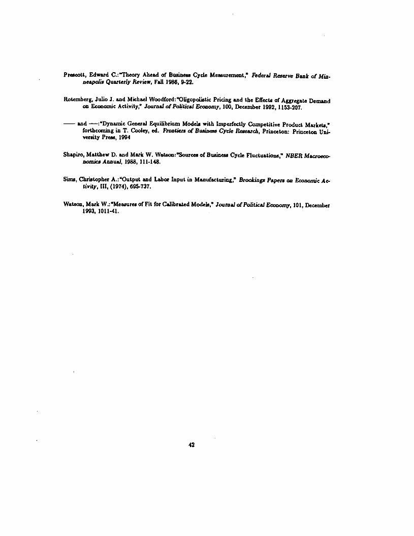
Prescott, Edward C.:Theory Ahead of Business Cycle Measurement," Federal Reserve Bank of Min-neapolis Quarterly Review, Fall 1986, 9-22.

Rotemberg, Julio J. and Michael Wood(ord:sOligopolistic Pricing and the Effects of Aggregate Demandon Economic Activity," Journal of Political Econonu', 100, December 1992, 1153-207.

— and —:"Dynamic General Equilibrium Models with Imperfectly CompetitiveProduct Marketa,"forthcoming in T. Cooley, S. hontien o(Businas Cycle Research, Princeton: Princeton Uni-versity Press, 1994

Shapiro, Matthew I). and Mark W. Watson:"Sourcn of Business Cycle Fluctuations," KEEn Macroeco-nomics Annual, 1988, 111-148.

Sbus, Christopher A.:Output and Labor Input in Manufacturing," Brookings Papers on Economic Ac-tivity, III, (1914), 695-731.

Watson, Mark W.:Meaaures ofFit for Calibrated Models," Journal of Political Ecooonv', 101, December1993, 1011-41.

42

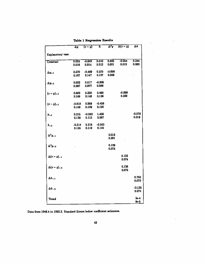
Table 1 Regression Results

Sy (c—y) ii My A(c—y) Ala

Explanatory van.

Constant 0.023 -0.042 0.0 10 0.005 -0.044 0.344

0.016 0.014 0.012 0.001 0.013 0.080

0.570 -0.469 0.570 -0.696

0.167 0.147 0_In 0.098

0.002 0.017 -0.0050.087 0.077 0.066

(c— v)—i 0.663 0.330 0.490 0.0980.166 0.146 0.126 0.030

(c — y)—i -0.618 0468 -0.4580.158 0.139 0.120

0.215 -0.283 1.450 -0.079

0.128 0.113 0.097 0.019

-0.314 0.316 -0.5030.135 0.119 0.102

0.0130.091

My_ti 0.1290.075

A(c— y)—a 0.1220.074

— v)—z 0.1260.075

Sh_1 0.7600.070

Ah_3 -0.1350.074

Thnd 3e-4Se-S

Data from 1948.4 to 1993.2. Standard Errors below coefficient estimata

43

Table 2Unconditional Second Moments

Moment Baseline Model U.S. Data

0.0053 0.0113

S.D.Sc/S.DAy 0.585 0.478

S.DAI/S.DAy 2.019 2.911

S.DAA/S.D.Sy 0.358 0.934

S.DAp/S.D.y 0.660 0.690

Con.(a.cAy) 0.987 0.5223

Corr.(Ah,Av) 0.917 0.7475

Corr.(4i,Ay) 0.994 0.9452

Con4Ap, âp) 0.994 0.4373

44

Table 3Estimated standaid deviations of forecAsted changes

it &A' 4' R!Horizon1. 0.0062 0.0023 0.0175 0.0077 0.0037 0.0094 0.308

0.0007 0.0004 0.0021 0.0005 0.0005

2. 0.0108 0.0044 0.0288 0.0130 0.0059 0.0148 0.347

0.0014 0.0007 0.0039 0.0013 0.0009

4. 0.0190 0.0082 0.0494 0.0204 0.0081 0.0220 0.429

0.0029 0.0014 0.0077 0.0029 0.0014

8. 0.0299 0.0139 0.0761 0.0309 0.0080 0.0273 0.550

0.0039 0.0022 0.0096 0.0045 0.0017

12 0.0326 0.0172 0.0825 0.0341 0.0072 0.0304 0.537

0.0034 0.0027 0.0068 0.0031 0.0018

24 0.0309 0.0224 0.0772 0.0323 0.0067 0.0394 0.384

0.0037 0.0046 0.0053 0.0012 0.0020

0.0310 0.0272 0.0585 0.0325 0.0068 0.000

0.0044 0.0089 0.0039 0.0000 0.0023

Standaid Errors based on coefficient uncertainty below estirnata

45

Table 4Estimated correlations of predicted output changes

with the reressorsRegressor: y, (c— yg) h,

Horizon:1. 0.597 0.214 -0.599

0.090 0.109 0.090

2. 0.530 0.3 12 -0.7930.095 0.132 0.077

4. 0.201 0.451 -0.9600.095 0.142 0.030

8. 0.009 0.53 -0.9950.062 0.127 0.007

12. .0.087 0.546 -0.9790.058 0.119 0.013

24. -0.093 0.544 -0.9780.058 0.171 0.012

00 -0.092 0.541 -0.9780.071 0.240 0.014

Standard Errors based on coefficient uncertainty below estimates.

46

flble5Estimated regression coefficients among fbrecaa ted changes

coat axj; &&j rt,Horizon:

1. 0.2537 3.7413 1.0922 -0.09220.0590 0.1376 0.1103 0.1102

2. 0.3119 2.6057 1.0741 -0.07410.0603 0.1406 0.1154 0.1154

4. 0.34-43 2.5299 0.9881 0.01190.0637 0.1463 0.1079 0.1079

8. 0.3678 2.4751 0.9964 0.00360.0595 0.1389 0.1098 0.1098

13. 0.3997 2.4008 1.0230 .0.02300.0614 0.1434 0.1134 0.1134

24. 0.4970 2.1738 1.0253 -0.02530.1212 0.2828 0.1215 0.1215

__ 0.5711 2.0008 1.0252 -0.02520.2358 0.5502 0.1375 0.1375

Standard Errors based on coefficient uncertainty below esthnaI.

47

TabLe 6The Calibrated Parameter,

Parameter Defined by Values Description

y. 1.004 Steady state growth rate of technology (per quarter)

'7.. 1.004 Labor force growth rate (per quarter)

so 0.70 Share of private consumption expenditure in privatevalue added net of govt. purchases

6 0.025 Rate of depreciation of capital stock (per quarter)

0.42 Share of capital costs in total teats

CXL I Elasticity of substitution between capital and hours

r Fx-4 0.01625 Steady state real rate of return (per quarter)or

1/.r 1 IntertemporaJ elasticity of substitution ofconsumptionholding hours worked constant

4 Intertemporal elasticity of Labor supply

0 .00732 Standard deviation of permanent tecbnology aback

Note: Except for rate of population growth, parameters displayed above p take the same values as in King,Ploeser and Rebelo (1988a).

48

Table 7Predicted standard deviation, of forecasted changes

Table 8Predicted regression coefficients among forecasted changes

49

s11—&jt it3Horizon:

1 0.0003 0.0001 0.0005 0.0003 0.0006 0.0053 0.0035

2 0.0006 0.0013 0.0010 0.0006 0.0012 0.0076 0.0065

4 0.0012 0.0025 0.0019 0.0011 0.0022 0.0109 0.0113

8 0.0021 0.0046 0.0036 0.0020 0.0041 0.0159 0.0176

12 0.0029 0.0063 0.0049 0.0027 0.0056 0.0200 0.0208

24 0.0045 0.0097 0.0076 0.0042 0.0087 0.0300 0.0224

0.0066 0.0141 0.0110 0.0060 0.0126 0.0000

Table 9The £flct of Varying the Pretceace Paraineten

o 'aw S.D..&j,' Con — y) Coa(&j,",h) IC oa on &j,: x0.6 0.2 0.0041 -1.0 1.0 2.0990 -0.1799 1.1799

0.6 1.0 0.0030 -1.0 1.0 3.1763 -1.0312 2.0312

0.6 4.0 0.0003 -1.0 1.0 39.0290 -27.9521 28.9527

0.6 10.0 0.0025 1.0 -1.0 -6.3574 5.2520 -4.2520

1 0.2 0.0039 -1.0 1.0 1.5827 -0.0978 1.0978

1 1.0 0.0035 -1.0 1.0 1.7813 -0.3018 1.3918

I 4.0 0.0029 .1.0 1.0 2.1460 -0.9193 1.0193

1 10.0 0.0026 -1.0 1.0 23765 -1.2504 2.2504

0.0023 -1.0 1.0 2.6845 -1.6862 2.6862

4 0.2 0.0031 1.0 -1.0 0.8975 0.0621 0.9379

4 1 0.0029 1.0 1.0 0.8854 -0.0488 1.0488

4 4 0.0029 1.0 1.0 0.8867 -0.0365 1.0365

4 10 0.0030 1.0 1.0 0.8869 4.0348 1.0348

I 0.0030 1.0 1.0 0.8870 -0.0337 1.0337

10 0.2 0.0022 1.0 1.0 0.6531 -0.0426 1.0425

tO I 0.0022 1.0 1.0 0.6680 -0.0281 1.0281

10 4 0.0022 1.0 1.0 0.6686 -0.0264 1.0264

10 10 0.0022 1.0 1.0 0.6587 -0.0261 1.0281

10 0.0022 1.0 1.0 0.6688 -0.0259 1.0259

50

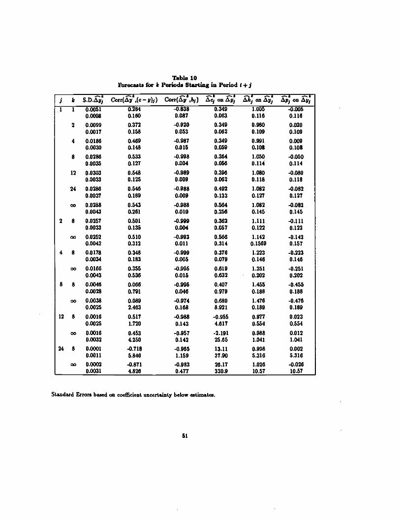
Table 10kbrecasts fbr b Period. Starting in Period t + j

j k S.Dsi,; Corr(&jt,(c —y)j) Corr(&jt,hj) r; xi,; xj.; xi; xi,;1 0.0051 0.284 -0.838 0.349 1.005 -0.005

0.0008 0.160 0.087 0.063 0.116 0.116

2 0.0099 0.372 -0.920 0.349 0.980 0.0200.0017 0.158 0.053 0.062 0.109 0,109

4 0.0186 0.469 -0.987 0.349 0.991 0.0090.0030 0.148 0.015 0.059 0.108 0.108

8 0.0288 0.533 -0.998 0.364 1.050 -0.0500.0035 0.127 0.004 0.056 0.114 0.114

12 0.0303 0.548 -0.989 0.396 1.080 -0.0800.0033 0.125 0.009 0.062 0.118 0.118

24 0.0286 0346 -0.988 0.492 1.082 -0.0820.0037 0.189 0.009 0.133 0.127 0.127

0.0288 0.543 -0.988 0.564 1.082 -0.0820.0043 0.261 0.010 0.256 0.145 0.145

2 8 0.0257 0.501 -0.999 0.362 1.111 -0.1110.0033 0.135 0.004 0.057 0.122 0.122

0.0252 0.510 -0.993 0.566 1.142 -0.1420.0042 0.312 0.011 0.314 0.1569 0.157

4 8 0.0178 0.348 -0.999 0.376 1.223 -0.2230.0034 0.183 0.005 0.019 0.146 0.146

0.0166 0.355 -0.995 0.619 1.251 -0.2510.0043 0.536 0.015 0.632 0.202 0.202

8 8 0.0046 0.066 -0.995 0.407 1.455 -0.4550.0028 0.791 0.046 0.919 0.188 0.188

0.0038 0.089 -0.914 0.680 1.476 -0.4760.0025 2.463 0.168 8.921 0.189 0.189

12 8 0.0016 0.517 -0.988 -0.955 0.977 0.0230.0025 1.720 0.143 4.617 0.554 0.554

0.0016 0.453 -0.957 -2.191 0.988 0.0120.0032 4.250 0.142 25.65 1.041 1.041

24 8 0.0001 -0.718 -0.965 13.11 0.998 0.0020.0011 5.846 1.159 37.90 5.316 5.316

0.0002 -0.871 -0.983 26.17 1.026 -0.0260.0031 4.826 0.477 330.9 10.57 10.57

Standard Errors based on coefficient uncertainty below ntimates.

51

Predicted Stands:

f*:

d Devia

1

Uon of

2

k PerIod 0

4

utput CLan

8 12

gsa Starting at I + .1

I 8 0.0020 0.0019 0.0012 0.0014 0.0012 0.0007[o 0.0063 0.0060 0.0054 0.0045 0.0037 0.0020

The Effect of SlowTable 12

Diffu.ion of Technical Progreu

ft S.DZP" IL' Corr(4'21c — y) Corr(t"h) &' on Lj, &i:' Li,:' Li,:'0.99 0.0001 0.990 -0.535 0.523 0.885 0.091 0.908

0.98 0.0002 0.975 -0.394 0.393 0.806 0.155 0.845

0.95 0.0006 0.827 -0.213 0.213 0.685 0.252 0.748

0.9 0.0012 0.695 -0.125 0.125 0.630 0.296 0.704

0.8 0.0022 0.409 -0.132 0.132 0.634 0.293 0.707

0.7 0.0027 0.256 -0.205 0.205 0.676•

0.259 0.741

0.6 0.0030 0.170 -0.304 0304 0.746 0.203 0.797

0.5 0.0032 0.118 -0.420 0.420 0.849 0.121 0.879

0.4 0.0033 0.083 -0.550 0.550 0.992 0M06 0.994

03 0.0033 0.059 -0.688 0428 1.191 -0.153 1.153

0.2 0.0032 0.041 -0.826 0426 L459 -0.367 1.367

0.1 t0030 0.029 -0.945 0345 1.798 -0.638 1.638

62

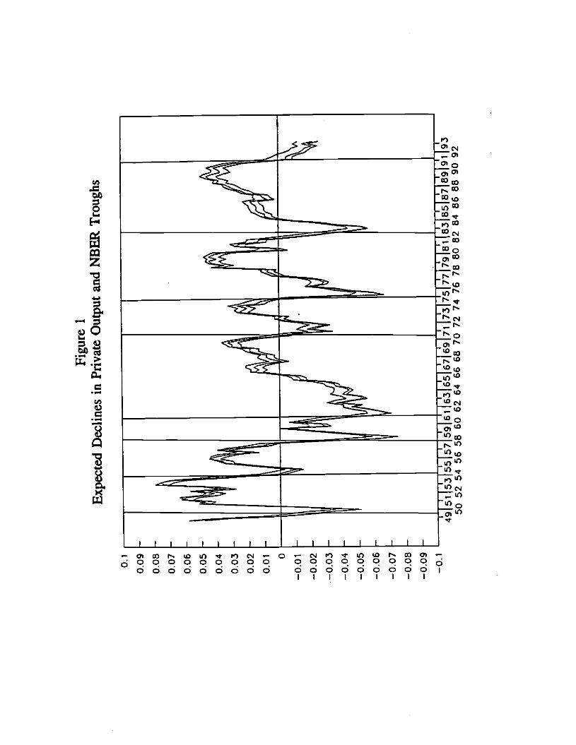
0.1

0.09

0.08

0.07

0.06

0.05

0.04

0.03

0.02

0.01

0

—0.

01

—0.

02

—0.

03

—0.

04

—0.

05

—0.

06

—0.

07

—0.

08

—0.

09

—0.

1

Figu

re 1

Exp

ecte

d D

eclin

es in

Pri

vate

Out

put

and

NB

ER

Tro

ughs

50 5

2 54

60

62

64 6

6 68

70

72 7

4 76

78

80 8

2 92

0.1

0.09

0.08

0.07

0.06

0.05

0.04

0.03

0.02

0.01

0

—0.

01

—0.

02

—0.

03

—0.

04

—0.

05

—0.

06

—0.

07

—0.

08

—0.

09

—0.

1

Figu

re 2

E

xpec

ted

Dec

lines

in

Nex

t 12

Qua

rter

s an

d D

etre

nded

Out

put

5860

6264

6668

707

2 74

76 7

8808

2 84

86

8890

92

0 ET

C O

P

PR

EF

I 2

Figu

re 3

A

1%Sh

ockt

oz; a=

1;e=

4 2 15

-

I.

CO

*..

I o:

l?:t.

* *

* . *

* +

*

* •

* t .

* *

t..*.

* t,

S •

S

S *

—

****

05

. .

.

++

+ +

+ +

+ + +

++

++

++

++

++

++

++

++

++

++

++

++

++

++

++

++

++

++

++

+ ++

++

+ +

++

H

ours

-0.5

-

I 10

20

30

40

50

60

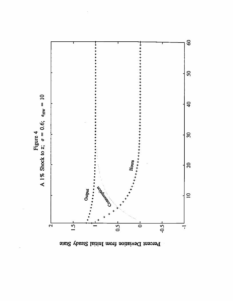
I I+t +• +• +• +* +• +* +• +

+ 0• + 0* +• +• +* +o +* +o * +• +¶ + .0• +• +• +* +• +* +'S +d +t +* + 00' • + cn

hdb +DO • +

::o *: +4— •: +

+

8 * 0(N

+b * +* +• +c * +

++

+ 0* 4 +o * +• o•.. +••

++

* +* +I I I

In 0 Ind

4os eqiuz wo.q uogw lU9OlOd

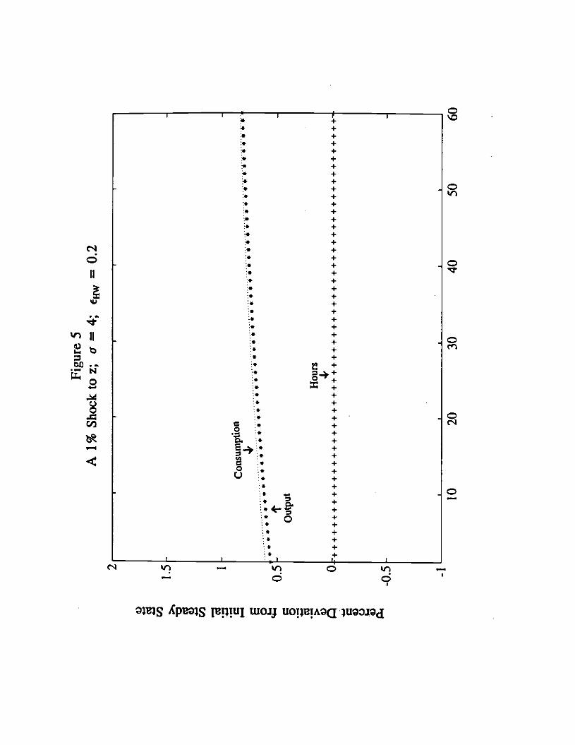
Figu

re 5

A

1%S

hock

toz;

o=

4; e

,,=O

.2

2

15

1L. 0.5

::::0

:...

.s

• 4

.. 44

4..o

Out

put

Hou

rs

4.

0 r+

++

++

++

++

++

++

++

++

+÷

++

+÷

++

++

++

++

++

++

++

++

++

++

++

++

++

++

++

++

++

+

.05.

—I

I

10

20

30

40

50

60

________ 0I I it I .1 0

S.4:4.4.S.. . 00't

C'.' 'S...o ten *— *

*4C.E

4 +•+4+•+4+5+I I I I,,4i— 'q. - c— — 0 0 0 0 9 9

OW3S AP8QIS !BI2IUJ UIO.IJ UOTIE!A9a 2UOOIOd