multiple regression with a qualitative dependent variable

Multiple Regression with a Qualitative Dependent Variable

Daniel L. Rubinfeld

The problem of scale construction has received considerable attention outside the discipline of economics.’ At the same time the use of maximum- likelihood estimation techniques such as probit and logit analysis to study qualitative choice problems has become quite popular. Within the purview of eco- non&s, relatively little attention has been paid to the relationship between scaling techniques and the analysis of models with qualitative dependent variables. This paper attempts to fill in some missing ground by stressing the link between multiple regression and models in which one seeks to determine a scale: to represent a qualitative dependent variable. We describe methods by which a single set of scores for the dependent variable can be estimated simultaneously with the coefficients of the “independent” variables of a model.2 Although the results may be interpreted in a multiple regression framework (e.g., as an extension of the linear probability model), we stress that the estimation technique need not involve multiple re-

’ The problem of scale construction has received substantial treatment in the statistics literature. One prooxiure similar to the scaling technique described in this paper was devised by Quttman (1941,1950). Guttman deals with the case in q.T.Gch the independent variables take the form of responses to a series of survey questions. Other discussions of scale construction appe;,: in Shepard, Romney, and Nerlove (1972) and Green and Rao (1973).

’ The search for a single wt of scores is a restrictive one and thus substantially limits the scope of our analysis. We shalt return to this issue later in the discussion.

From the University of Michigan, An? Arbor, Michigan. Address reprint requests to Dr. Daniel L. Rubinfeld, Associate

Professor of Economics and Law, University of Michigan, Ann Arbor, Michigan 48109.

Journal of Fxonomics and Business 34.67-78 ( 1983) @I 1982 Temple University

However, tbe paper goes 00 to show an iterative kost-

squadfs multiple qresshm technique can provide a

lfidbl~tbntotbeaelnore~dpracedrws.

TIK tcctuaiques orr! ilhstmted witE3’labor force participation md voter hmout examples.

gression calculations. Because most of these techniques involye nonlinear estimation techniques that can be time-consuming and expensive for large data sets or large models, we propose an ad hoc multiple regression scaling technique that is relatively inex- pensive to use. The multiple regression technique provides a useful approximation of some of the more general multivariate statistical techniques.

Assume that we know that a given individual unit of study, family, firm, city, and so on is characterized by a vector of attributes. Each individual population member is assumed to belong to one ;bf severat mutually exclusive groups, and the attribL . va:;ars associated with each group are known to hz c>imafIj/ distributed with different means but ;de~?tl~~~l variance-covariance matrices. The problem % to l? ! a single linear decision rule that predicts the grc .F “score” of an individual after the vector P .r~trib~. :es describing that individual is observed. The Cndicted group scores can be interpreted as provi?ing f01 a qualitative “‘dependent” variable in a multiple regression procedure. The predicted scores also provide for a method that allows for the classification of individuals into groups. The procedure is related in terms of distributional assumptions to slultiple discriminant analysis and is identical when thr scimple means of the group attribute vectors lie on a straight line.

The techniques described here should be of use in economics as well as in related social science disci-

plines. Examples of some relevant applications are as

follows: 1. In survey analysis, respondents to a question-

naire might be classifkd into one of several

67 0278-2294/82/O I /067- 12$2.75

68 D. L Rubinfeld

groups (e.g., Agree. Disagree, No response). ,%ttribute data are available for each of the respondents and al I respondents in each group arc astuned to be drawn frorI1 a population with the same mean attribute vector. One can attach a score to each of the groups in an attempt to determine whether those who do not answer a given question are mQre like those who agree or more Lae those who disagree.

2. In a study df the work status of a certain segment of the labor f~irce. one may wish to emphasize the dtstinc!lon between those who work part-time and those u,ho work full-time. If the individuals sampled can be properly classified into distinct groups such as unemployed, part-time employed, and full-time employed, and if attribute and labor market data are available, the scaling technique t’dn provide a useful mode of analysis. The technique will be particularly valuable if one wishes to determine those individual attributes that best distinguish between the labor force categories.

3. Assume that corporate r.r municipal bond ratings have hcen attached to a list of bonds to be studied.’ The scaling procedure can be used in an attempt to replicate the behavior of the rating agenclcs. One can determine weights for each of the attributes that determine ratings as well as a quantitative Score for each of the rating cate- goxs. Classificaticn rules can be obtained and ued in the sample to test the validity of using a \tngle ilncar decisions rule to describe the rating p0LX%.

I-he remainder of the paper is divided into five sectIons_ The first introduces the formulation of the multiple regression model. with the unkr,awn group KOI-,LY~ Interpreted artificially as the dependent I arlable in the regression model. Least-squares mini- mvation subject to a constraint on the estimated parameter!, Eeads to the simultaneous determination ~uwn;! cigen\ectors and eigenkalues) of a set of group \icrres and the Heights attached to the vector of Indl\ldual attributes. The second discusses the interpretation of the regression model with particular cmphasls on its use lor classification purposes. Tkc: third dexxbes an alternative vie% c4 the identical xoring problem through a generalized analysis C,I \ arlance approach. Tlx fourth describes a met hod by ti hlch ordinar! least squares can be used to er.timate the dependent variable scale and the attribute

weights. The fifth contains two examples of the application of the ordinary least-squares regression technique.

GROUP SCORING IN A MULTIPLE REGRESSION SFXTING

We assume that each individual unit under study is represented by an attribute vector, and that the popu-

lation of attribute vectors may be partitioned into G groups. We also assume a quantitative score rs can be attached to each group, with no presumption that tne 31,s will ;lecessarily be distinct. We proceed in this section to determine a set of scores and attribute weights that minimize the sum of squared residuals of an artificially defined regression problem. We stress the artificiality of the procedure because the ‘de- Fndent” variable is not known and is clearly not normally distributed. We shall see that the multiple .-egresiion approach yields a technique that is identical to other ad hoc scaling procedures computation- ally, and has the advantage of providing a useful means of interpreting the estimated scale and attribute weights

We define tl unknown dependent variable y ah follows:4

x1 if the observation is in group ‘.

!lr= CI~ if the observation is in group 2

LX(; if the observat!qp is in group C;.

(O

f= 1. 2. ***, N

There are .V!, observations in each of the S groups, and a total of N observations in the sample.

It will be helpful to represent the vector J as the product of a grouping matrix and a vector of unknown scores. i.e.,

where

31=\x,. *.., xc;)’ (1 G x 1 vector

- _--

a None wcrc able to specify a priori the probabilities with which

J, takes each of the G possible values. then further pursual of a linear

probability nt .~del approach? might be juGed. The linear probability

mcxki IS desccnbeci in Ladd [XJ. An attempted extension of the linear

probanllit~ appears in Warner [ 123. Since our primary olz_lpctive 15 to

e:stImatc a set t)f scores or scale that can be interpreted in a rt,-&on

setting, we shdll proclz in a different direction.

Multiple Regression with a Qualitative Dependent Variable 69

,+y”. . . .* D”‘j an A x G matrix

D(cl’g= i.z.-.* . G = 1 if the observation is in group p and 0 other. ise.

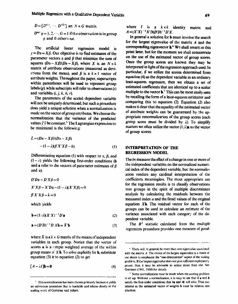
The artificial linear regression model is _V = DZ = X/I. Our objective is to find estimates of the parameter vectors z and fi that minimize the sum of squares (Dr -Xfi)‘(Dr - X0). where X is an N x k matrix of attribute observations (measured as devi- Ptions from the mean), and Iy is a k x 1 vector of attribute weights. Throughout the paper, superscripts within parentheses will be used to represent group labels (g), while subscripts will refer to observations (1) and variables (i. j, k, h, r).

The parameters of the scaled dependent variable will not be uniquely determined, but such a procedure does yield a unique solution when a normalization is made on the vector of group attributes. We choose the normalization that the variance of the predicted values $f be constant? The Lagrangian expression to be minimized is the followirq:

L=(Dr--Xfl)‘(Dr-X/3)

- (1 - i)(B’X’Xj? - k). (1)

Differentiating equation (1) with respect to 01, Iy, and (1 -i) yields the following first-order conditions (b and a refer to the vectors of parameter estimates of /? and a):

D’Da - D’XP = 0

X’XjV-X’Da-(1 -i)(X’XjY)=O

/3’X’Xp--k=O

which yields

b=( 1 /i)(X'X)- ‘D’a (2)

a=(D’D)-‘D’Xb=X’b (3)

where X is a k x G matrix of the means of independent variables in each group. Notice that the vector of scores a is a f.imple weighted average of the within group means o’ X b. To solve explicitly for b, substitute equation (3) ir to equation (2) to get

[A -il]b=O (4)

5 This normslization has been chosen primarily because it yields an estimation procedure that is tractable and relates closely to the scaling work of Guttman and others.

where I is a k xk identity matrix and A =(x’x)‘-‘x’~!I(D’D)-‘D’x.

In general a solution for b must involve the sear& for the largest eigenvalue of the matrix A and the corresponding eigenvector b? WC shall returnaa this point later, but for the moment we sbaEl con&ntrate on the use of the estimated vector of group scores. Once the group scores are known they may be interpreted in light of the regression approach used. In particular, if we utilize the scores determined from equation (4) as the dependent variable in an ordinary least-squares regression, then we obtain a set of estimated coefftcients that are identical up to a scalar multiple to the vector b.’ This can be most easily seen by recalling the form of a least-squares estimator and comparing this to equation (2). Equation (2) also makes it clear that the equality of the estimated vector of attribute weights can be guaranteed by the appropriate renormalization of the group scores (each group score must be divided by A). To simplify matters we often utilize the vector (1 /@I as the vector of group scores.

INTERPRETATION OF THE REGRESSION MODEL

The bs measure the effect of a change in one or more of the independent variables on the normalized numerical index of the dependent variable, but :he normalization renders any cardinal interpretation of the coe!Iicients meaningless. The most appropriate use for the regression results is to classify observations into groups in the spirit of multiple discnminant analysis by calculating the residuals between the measured index Q and the fitted values of the original equation Xb. The residual vector for each of the groups can be used to calculate an estimate of the variance associated with each category of the dependent variable.

The R2 statistic calculated from the multiple regression procedure provides one measure of good-

h There will, in general, be more than one eigenvalue askated with the matrix A. The choice of the largest eigenvalue is a result of our desire to emphasize the ‘one-dimensional” aspect of the scaling problrm. If tile largest eigenvalue does not give sulkient explanatory power, then it may be advisable to utilize more than one. See Guttman (1931, 1950) for details.

’ Some normalization must be made when the scoring problem is set up. Without .I normalization, it is easy to see that if a wd b satisfy the first-order conditions that &a and kk will also. Thus our inteKst in the estimated vector of weights b must be relative, not

absolute.

70 D. L Rubinfeld

ness of lit of the scoring procedure. R2 measures the proportion of the variation in y = Da explained by the variation in the w~@:ted average of group attributes Xb. The calculated R2 will be identically equal to k, the value of the largest eigenvalue of the matrix A in equa?ion (4). This follows directly from the fact that

t’X’Xb R’= ._

b”X’Xb = -Ye

y ’ y a’D’Da

where a has been renormalized so that:

i, t. ;

Then

r R'

1

b’X’Xb - = i _ _-. - __- -.-_ 1 b’i’D(D’k)- ‘D’XbJ

= i from equation (4)

Perhaps a more proper measure of success of the procedure would involve a comparison with alternat-

ivc techniques ti2f estimation and classification. One reasonable approilch would be to compare the multi; le regression classification errors with the number of classification errors associated with a multiple discrimiriant analysis procedure. This measure of success is daptive, because multiple discriminant analysis involves the estimation of G - 1 independent equations, and thus uses more degrees of freedom than the regrcssiol technique.

GROUP SCORING IN AN ANALYSIS OF VARIANCE SETI’ING

The group Ncaling or scoring problem has frequently beep described in the literature in terms of generalized analysis of variance and canonical correlation. We shall describe the former approach here and leave the latter derivation to the reader.’ Assume that we wish to find a vector b which maximizes the variance among group means relative !o the total varianclt within groups. To accomplish this we define

1. S = (S,,) = matrix rif pooled sum of cross-product:; using deviations about overall means

--_-- --

* E or further deta& ccmcernmg borh approaches, see Gurtman I !UW. 4ndersun I 1958~ Cooiej and Lohnes (1962, 1971 J, am? Rao 4 iuii,‘a

2.

where X(e) refers to the N, x k matrix of observations associated with the gth group.

Then with variables mesured as deviations about means S= X’X, C =(Cij)= matrix Of pOOled sum Of CrOsS- products using deviations about within group means

Then

C=X'X-X'D(D'D)-'D'X.

The variance among group means can be represented by b’Yb where

b'=S--C=X'D(D'D)-'D'X,

while the total variance is given by b’Sb. We can maximize b’Vb subject to b’Sb being

constant by writing the Lagrangian

L=b’X’D(D’D)- ‘D’Xb-i(b’X’Xb-k).

Diflerentiating with respect to b and solving we obtain

X'D(D'D,- ‘D’Xb=iX’Xb

or

(A - E.Z)b=O (6)

where ,4=(X’X)- 'X'D(D'D)-'D'X and J is a k x k identity matrix. This can be seen to be identical m form to equation (4). The soLon to equation (41 is once again obtained by choosing the largest eigenvalue i. (which satisfies the constraints).“

’ Nor infrequently the derivation just described is given as one that maximizes b’Vb subject to b’Cb being constant. The attribute weight> and group scores obtained will be equivalent up to a scalar multiple, but the ne* eigenvalue obtained will not be equal to i. In particular, it IS possrble to show that O=i,/(l +A) where 0 is the eigenvalue of the matrix c’- ’ V. See Cooley and Lohnes (1971) for some details. This has relevanLz here because the canonical correlation package used in the application provides an estimate of 8, not

Multiple Repssian with a Qualitative Dependent Variable ‘81

ORDINARY LEAST SQUARES WITH A QUALITATIVE DEPENDENT VARIABLE (OQDV)

The scoring procedure just described su@ers from the disadvantage that a solution cannot be obtained using a standard multiple regression package. In this section we briefly outline an estimation process that will enable us to obtain an estimate of the vector of weights fl (and the scores a) using ordinary least squares.

Recall that the original formulation of the model was Da = X#YI. We can utiliz ordinary least squares by normalizing the vector a, arbitrarily choosing a 1 = 0 and uG = 1. Ordinary least-squares estimation can be used if we rewrite the model in the following form:

B f \ U2

pqx _~‘2’_~‘3’_....4yG’- I’) f3 .

\ /

.

aG-1 *

(7)

The least-square% technique applied to equation (7) provides for an estimate b of the parameter #I. The estimated scale is simply the vector a = R’b. There is no guarantee that the estimation procedure will yield 3 scale consistent with one’s prior notions about the ordering of the groups. More importantly, there is no guarantee that OQDV will yield scores identical (up to a suitable transformation) to those derived earlier. This can be realized intuitively by noting that the calculated scores for all groups other than the 1st and Gth will be identical to those obtained by the ordinary least-squares procedure. But the scores for the 1st and the Gth groups will not necessarily equal 0 and 1, respectively. lo

The scale estimate obtained for the set of group scores can be used to obtain improved parameter estimates through the use of an iterated least-squares procedure. The second iteration is accomplished by regressing the vector Da on the vector of attributes X. This will yield a new set of estimated attribute weights b’ and a new set of group scores a’. Then the new group scores yield a new set of attribute weights, and so on. The iterated set of group scores and attribute weights will remain unchanged frcjm the previous set only when the esti,mated scale and weights co’rre-

I’ The estimated scores will be equivalent to those derived carlier when the sample means of the ,t’:ibute vectors lie on a straight line. See Appendix for proof.

spond to the generalized analysis 0;” variance solution (and when the R2 is identically equal .to the eigenvalue of the matrix A). We have been unable to prove convergence under a geileral set of conditions, but the lack 0: a general set of cc?vergence conditions is not likely to be of practical consequence. The reason is that when convergence does occur, the estimated scale ipnd weights will correspond to the generalized analysis of variance solution, with R2 being equal to the largest eigenvaluz of A. And conversely when the scale is equal to the analysis of variance scale, the iterative process will end-additional iterations will yield the same scale. * I Thus convergence guarantees that the “‘optimal” solution has been reached, whereas nonconvergence will be rapidly apparent if it occurs. In practice, in a number of experiments conducted with different data sets, the estimated scale converged rapidly with the genera&& analysis of variance scale.’ *

We have chosen to focus on a single linear function of the group attributes, but the techniques discussed should be viewed as a special case of the more general decision rule used for multiple classification. In fact, the scoring procedures (both OQDV and the more general iterative procedure) can be shown to be identical to multiple discriminant analysis when the sample group means of X lie on a straight line. ’ ’ This suggests a set of conditions under which the use of a single set of group scores involves no loss of explanatory power as well as the conditions under which OQDV is likely to approximate closely the more general scoring procedure.

Statistical Testing

As a final item, it is reasonable to ask whether the statistical tests associated with the ordinary least- squares regression are valid in the scoring procedure described in this paper. Assume that we are working

- --

’ ’ Recall that the scale is a = S'b. II e dependent variable is Da and the regressor b. The newly calculatcL coellicient vector is then

v=(,y XI- ‘x’h=(x’x)- ‘X’DR’b

=(X’X)-‘X’D@‘Dj- 'D'Xbr rib.

Fram equation (4). if b is the g:neralized analysis of variance solution (/1- il)b= 0. Therefore b* = db = ib, so that I9 is a scalar multiple of b.

” The initial set of group scores obt tined will depend on the ?articular O-1 normalization chose. This zan be seen most clearly *Nilen the labor force example is discussed below.

* 3 A &t&d proof of this result is given in the Appendix.

72 Al L Rubinfeld

under the set of conditions described by multiple discriminant analysis (the Xs are assumed to be joint- normally distributedj. Then it is clear that under the condition that the true means of the group attribute vectors lie on a straight line, the distributional results of multiple discriminant analysis ho!d.‘4 In this case, small sample tests are appropriate, but since the conditions of the previous theozem are likely to hold approximately at best, any tests based on the meth- odology of discriminant analysis are Xikely to be inexact. If we view the scoring model as an approxi- ma!ion to the logit or probit model, large sample tests can be appropriate.

IWO EXAMPLES

L&or Force Particiption

The following application is b$ased ori a study of the labor force participation of married female teachers.’ ’ Ths focal point of the study was the breakdown of labor supply status into three croups----those working full-time. those working part-time, and those not working at all. One of the objectives of the study was to determine those variables that best help to distinguish between the three labor force groups. Discriminant analysis (two types) was the sole tech- luque used.

CJsing the same data set. we have attempted to cztimate a scale of set of scores for the three labor force groups. A brief description of :!he data set and a list of the relevant variables appear in Table 1. The reader is refer::d io the original source article for more sompiete details about the d;ata set.

Tables 2.3, and 4 contain the results of several of the e,.:imation experiments. Each of the scales listed in Table 2 was renormalized (through an appropriate ailine transformation) to mlake the results of the alternative estimation procedures comparable. Such a renormalization has no effect on the relative magnitude of attribute coeficients and no effect on the statistical tests esed. The complete multiple regression results for three of the experiments are !i:;ted for illustrative purposes.

Scale 1 was determined from a canonical corre- laGon package as a solution to the original scaling problem, The regression results using Scale 1 to form the ordered dependent variable are given in Table 3.

!’ Thewz tests are described in some dctall b> Anderson (1958)

anil RdC I1952).

TABLE 1. Definition of Variables

Sample* 414 married women consisting of 254 full- time teachers, 118 substitute teachers and 42 nonwork- ixlg teachers

Wsi = part-time wage of wife in $1000

WV9 = full-time wage of wife in $1000

WWI = wage of husband in $1000

T = household age in years

ASbTETS = household assets in $1000

##cH = number of children under six years of age

Dl = dummy variable equal to 1 if not working and zero otherwise

02 = dummy variable equal to 1 if part- time and zero otherwise

03 = dummy variable equal to 1 if full- time and zero otherwise

Source: Gramm (1973).

What value does such a scaling procedure have in the

context of this labor force problem? First, recall that the implicit assumption here is that one set of regression parameters can be used to explain the full- time, part-time, no work decision. Given this assumption, the estimated sca!e of 1,0.77,0 suggests that the characteristics or attributes of part-time workers ;s such that they are more similar or like those not working than those working part-time. This may hzve implications for policy not apparent in the C;ramm study because it suggests that labor force participation responses to policy changes may be substantial as workers move into the labor force to part-time jobs and out of the 1aMr force with relative ease. The regression results themselves make it much easier to evaluate the importance of individual characteristics in explaining the ordered labor force choice. The use of asymptotic tests in Table 3 allows us to say that the full-time wage of the wife has a significant positive effect on the probability of the woman’s entrance into the labor force (recall that 1 represents the nonworking choice). Significant but in the opposite direction is the wage of the husband, as one would expect. ‘41: of the coefficients have the f=xpected sign, and only one is insignificant at the 10 percent level. The overall results suggest that taking into account the part-time status of women teachers does not alter the behavior that would !x predicted by labor economics theory. These results are also im- p!icit in the more genera! discriminant analysis approach, btkt the multii4e regression does simplify the analysis. in OH case, the lost precision or

Multiple Regre&m with a Qualitative Dependent Variable 73

TABLE 2. Scale Variables Defined’

Labor Force Status Scale 16 Scale 2C State 3d Scale 4e Scale Sf Scale 68

Not working

Part-time

Full-time

1 .ooo I.000 1 .ooo 1 .ooo 1 .ooo 1.000

0.770 0.858 0.662 0.399 0.699 0.757

0.000 0.000 0.000 0.000 O.OGO ’ 0.000

’ All scale variables have heen renormalized for purpow of comparison by means of suitably chosen afke transformations. * Obtained through the solution of equation (6) using canonical correlation computer program. ’ Obtained by regression of D2 on Dl.

d Obtained by regression of D3 on D2. 6 Obtained by regression of Dl on 03. I Obtained through second iieration using least-squares regression of Dl on D3. ” Obtained thr0uB.n third iteration using regression of Dl on 03.

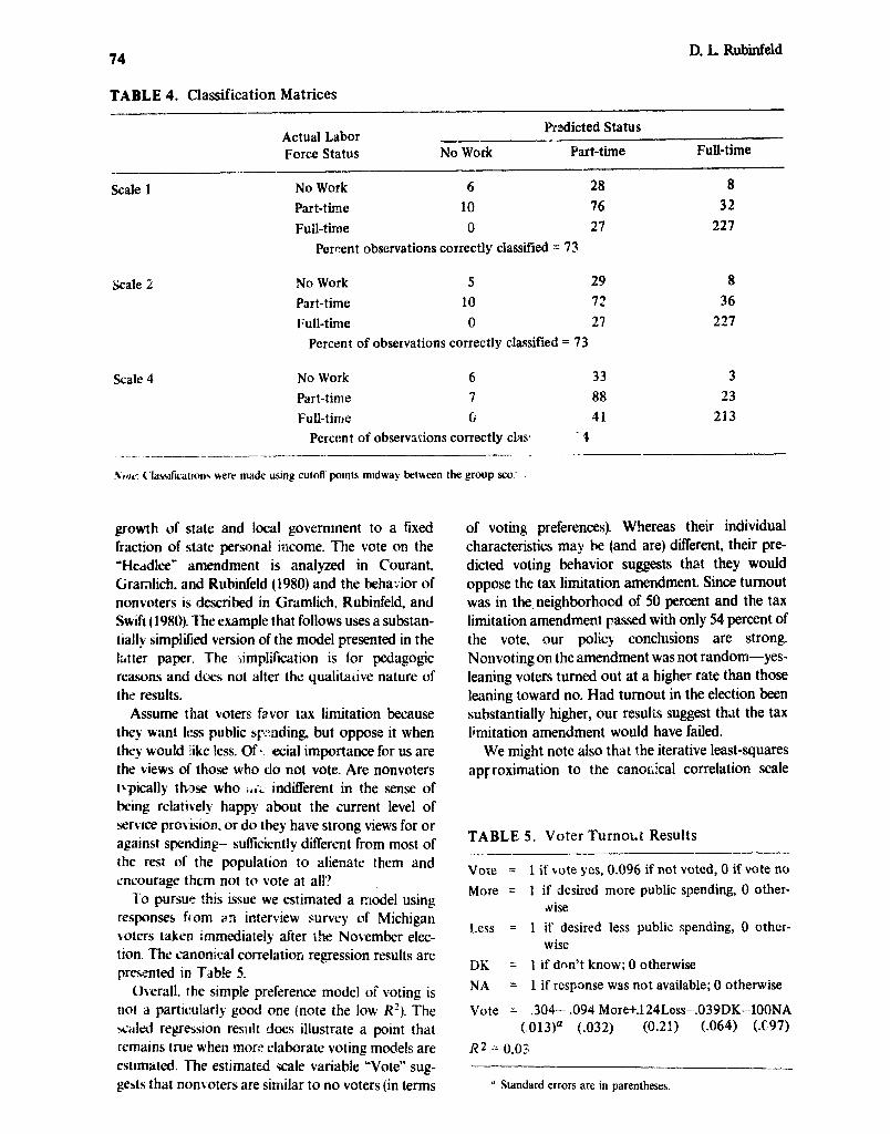
explanatory po~ver of the model is small, since our results predict almost as well as do those obtained from the multiple discriminant analysrs approach.

How does our iterative least-squares approach to estimation work in this case? To evaluate this question, the remaining scale variables were ob’rinti using the OQDV approximation and a stan&d multiple regression package. What is most striking about the OQDX approximation is the degree of accuracy associated with the first iteration of the procedure. The Scale obtained through the regression Dl on 03 and the vector of attributes (-kale 4) yields the poorest results, but even in this case W2 is only 0.04

below the maximal R2, all signs are identical, and only one additional coefficient (the r variable) is insignificant. When the Scale 4 variable was used iteratively to obtain new scale variables I’&aie 5 and Scale 6) the results were again very promising. By the third iteration the difference in scales was small and no substantive difference in regression results could be seen.

Voter Turnout In the 1978 congressional election, Michigan voters passed a tax limitation amendment that limited the

TABLE 3. Regression Results

Constant W(S) W(F) W(H) T Assets

Scale 1

(St. Err.)

0.422a -0.0063 -0.056a 0.018’r 0.0045= 0.0013b 0.35@

(0.116) (0.022) (0.008) (0.002) (0.0020) (0.0007) (0.035)

I?* = 0.443 S.E. = 0.308 Percent variance exv-lained by Crst eigenvalue = 91 .l

scale 2

(St. Err.)

0.4w -0.006 1 -0.06 la 0.019a 0.0054a 0.0014b 0.370a

(0.124) (0.024) (0.009) (0.002) (0.0022) (0.0007) (0.037)

I?* = 0.442 SE. = 0.330

Scale 4

(St. Err.)

0.279a -0.0072 -0.035” 0.013~ 0.0005 0.0010b 0.3ooa

(0.094) (0.018) (0.007) (0.002) (0.0016 j (0.0005) (0.028)

R* = 0.399 S.E. = 0.250 -

Notes: 1. The standard error is an estimate. 2. Regression coeffkients and standard errors of the regression are not directly comparable, since the variance of the dependent

variable has not been fixed. 3. The results of Scale 1 are not identical (up to a scalar multiple) to those given in Gramm (1973). owing most likely to an errof ln the

transmission of the data. ’ Signilicant at the 5 percent level (using standard r test). ’ Significant at the 10 percent level.

74 D. L Rubiield

TABLE 4. Classification Matrices

Actual Labor Prsdicted Status

Force Status No Work Part-time Full-time

Scale 1 No Work 6 28 8

Part-time 10 76 32 Full-time 0 27 227

Percent observations correctly classified = 73

scale 2 No Work 5 29 8 Part-time 10 72 36 Full-time 0 27 227

Percent of observations correctly classified = 73

Scale 4 No Work 6 33 3

Part-time 7 88 23

Full-time G 41 213

Percent of observations correctly clas ‘4 _ ._

.Colt- ~‘ladic~~~ons were made using cutoff pods midway between the group sco-s

growth of state and local govermnent to a fixed fraction of state personal income. The vote on the “Heddlee” amendment is analyzed in COurant.

Granlich. and Rubinfeld (1980) and the beha;-ior of nonvoters is described in Gramlich, Rubinfeld, and Swift ( 1980). The example that follows uses a substantially simplified version of the model presented in the lstter paper. The simplification is for pedagogic reasons and dcej not alter the qualitalive nature of the results.

Assume that voters favor tax limitation because they want less public sy:tnding, but oppose it when they would iike less. of Y ecial importance for us are the views of those who do not vote. Are nonvoters tkpically those who ,,r‘~’ indifferent in the sense of being relatively happy about the current level of servtce provision, or do they have strong views for or against spending-Psu&iently different from most of the rest of the population to alienate them and encourage them not to vote at all’?

To pursue this issue we estimated a model using responses from a:~r interview survey of Michigan voters taken immediately after the Nov*ember election. The canonical correlatioii regression results are pre_vted in Tdb!e 5.

Overall. the simple preference model of voting is

not a particularly good one (note the low R’). The *tiled regression result does illustrate a point that remains true wheu more elaborate voting models are estimated. The estimated scale variable “Vote” suggests that nonvoters are similar to no voters (in terms

of voting preferences). Whereas their individual characteristics may be (and are) different, their predicted voting behavior suggests that they would oppose the tax limitation amendment. Since turnout was in theneighborhood of 50 percent and the tax limitation amendment passed with only 54 percent of the vote, our policy conclusions are strong. Nonvoting on the amendment was not random-yes- leaning voters turned out at a higher rate than those leaning toward no. Had turnout in the election been substantially higher, our results suggest that the tax limitation amendment would have failed.

We might note also that the iterative least-squares spy roximation to the canoriical correlation scale

TABLE 5. Voter Turnout Results

Vote = 1 if bate yes, 0.096 if not voted, 0 if vote no

More = 1 if desired more public spending, 0 other- &e

Less = 1 if desired less public spending, 0 otherwise

DK = 1 if don’t know; 0 otherwise

NA = 1 if response was not available; 0 otherwise

Vote = .304- .094 More+.l24Less--.039DK-lOONA (013)” (.032) (0.21) t.064) (X197)

R2 = 0.03 ..-

’ Standard errors are in parentheses.

Multiple Regression with a QuaEtative Dependent Variable 75

converged rapidly to the solution. To obtain the scale, we regressed a yes-no dummy on the right-hand variables including a nonvoting dummy ant’ ijbtained an estimrated scale of 1, 0.155, 0. Using this scale to form a new dependent variable, we estimated a new regression and formed a new scale, 1, 0.102, 0. The third iteration yielded a scale of 1,0.0!96,0, essentially the same as the canonical correlation scale. For large models, this iterative technique can save substantially on computer cost.

CONCLUSIONS

We have described a procedure whereby a set of scores or scale for a “dependent” variable can be estimated simultaneously with the coeficients of the independent variables of an equation. Although the estimation procedure involves the search for the eigenvaiues of a matrix, the resulting scores and

attribute weights may be interpreted in a regression

setting. The scale for the dependent variable provides the basis for a decision rule that allows for the prediction or ciassifcation of individual observations into categories and also provides for a measure of success oft he regression procedure. We have seen that the scaling procedure can be viewed alternatively as a process that involves the maximization of the among group variance relative to the within group variance. The resulting scale is equivalent to one that would be obtaine j by the suggestd scaling techniques of Cuttman and others.

The ordinary least-squares regression package can be used to approximate the scale obtained through the previously discussed te&nique. The OQDV regression technique and the more general scaling procedure are seen to be equivalent to multiple discriminant analysis when the me;lns of the attribute vectors for each category lie on aI straight line in attribute space.

There are several limitat ions to the kind of scaling procedure described in this paper. A decision must be made as to whether an inllerently ma.lltidimensional problem should be reduced to an unidimensional one. The benefits of determini,ng a single linear set of weights for the group attributes and interpreting the calculated scores in a regression frarrlework may be outweighed by 5s costs associated with the loss of predictive power in the model. If the decision to :lse a single linear function is made, a choice of compu- tational techniques is avaiksble. The WVD technique has the advantage of simplicity of computation, but it may cause misleading resLJts if the assumption that the sample group means ire on a straight line is not

approximated. Further research is needed into the convergence properties of the iterative least-squares procedure a:, well as the tradeoffs involved in the choice of a one-dimensional scaling objective.

The author wishes to thank Franklin Fisher for stimu- lating his interest in this problem. Franklin Fisher, W. Locke Andeison, Saul Hymans, and an anonymous referee made helpful comments at several points in the developnlent of the paper.

APPENDIX

The relationship between the iteratitle least- squares scale estimation procedure @QED) und multiple discriminant analysis.

In the discriminant analysis appro& ior the multiple group case (and equal costs of misciassifi- cation) the attribute vectors associated with each group are assumed to be normally distributed with di3’erent means but identical variance-covariance matrices. Let J.P be the mean of X in group and Z the variance-covariance matrix of X and let X =(X( 1 ‘XC’, . . . . P’)’ where Xc+’ is an N,, x k matrix forg=1,2;.., G. Taking the logarithm of the ratio of the probability density functions for two arbitrary groups, one can obtain regions for classification. The decision rule that minimizes the t ,osts of misclassifi- cation involves the evaluation of G(G -- 1);2 func!:ons in which ail pairwise comparisons of groups are :,lade. These functions are as follows:

D,,,j X) = [X - ()P” + p) /2]

x c - I(p _ #I’)

From these discriminant functions hyperplanes are

calculated that span a(G - l)dimensionzl,space. lfthe u priori probabilities of an observation fatling into any category are equal, then the ciassificatidn rule is to place an observation in category g if t),,, I~z 0 for all h.’ In actual practice Fampie estimates of the true ,u’~’ and Z must b; utilized.’ Wifh this background, ie is now

’ For ;I complete deri\arlon utllrzmg 1111s approach. ~CC

Anderson (195X).

L The matrix of pool4 sum of cross-products usmg de\ra!lons

&our within group meims C can be used to obt;un a consistent

estimator of the unknown variable coiarian@matrix E:.

76 D. L Rubinfld

possible to compare multiple discrininant analysis with our scoring processes.

Corollary. If the means of the groups lie on a straight line (i.e..

km- 1. if Xc@. the mean vectors of earh of‘ the mceg~rius._fdl on a straight dine (in the parameter spuce), then the discriminant anaivsis hyperplanes ure parallel and only one discriminant function is needed to represent the process.

PROOF, The fact that the means lie (3n a straight line may be written algebraically as x(g)=7 +k,6 where the A, are scalars and 6,~ are vectors. The discriminant functions to be calculated may be written

(x@‘=y+k,&) then Cii=Sij-Q2(R!IJ-~12’)

x (y- q’) W)

where Q2 is a scalar and @ lb, Xi1 1, and Xi2), Xi21 are

the means of the ith and jth variables in thefirst two categories.

PROOF. If the means lie on a straight line then for any groups h and r,

~,,(,y)=x’(-- ‘(x-p’) (Rlh'-~~')=Qh,(X~1)-X12')

[(k”“‘+ p) ,q(‘- ‘(A 19)__ jf’h’) 642) where the second term of the equation is a scalar

whert

representing the intercept of the hyperplane. kh--k, Substituting for P and xth’ in the equation above, Q/W= ri-

we find that ‘I- ‘2

(A6)

Then

Since ihe k,s are scalars and the second term is a .scaIar. all D,,,s will sepresent parallel hyperylanes. Only one discriminant function and a set of cutoff points or rules is neecfed for the cOassificstion pro- c&ure. The coeflicients in the discriminant function D,JX) may be u,ritten as C-‘(Xt”-X’2’). c‘oefficients in &,( ,% ) may be represented as QJ’ ‘(A”“-- x”‘) where Qgh is a scalar whose value depends on g and h. Coeficients in each discriminant ftinction are a scalar multiple of coefficients in every other discriminan t function.

One final lemma is necessary to make comparisons possible between the regression techniques and multiple discriminant analysis.

LA

! i”’ =the tth observation of the gth group

ct= 1, 2. *-*. N, and g= 1, 2, Y G

(; In discriminant analysis the pooled cross-products

of deviations of A’, and X, about the within class means are used tL3 approximate I: ( i and j represent Independent \ arrables here). B!tt ordinary least squares &I\-elves the use of pooled cross-products of de\ iations of X, and X, about the okerall mean oft he Fample. To cornpap; discriminant analysis with O@X’. a lemma relating thtw two matrices is

j+=mean of _v= c cr,N,/N 9= 1

S,,.=covariance of y with *Yi.

neces.QrJ. Since the lemma is standard in the analysis Lemma 3 o,f \ariancc litcisturc a proof is not presented here.”

Lvinma 2 $.,.=(I N) i ; N,,Nr(~~,,--~+)

/I= I r= 1

( ._ = s,, _ ; i &J;, &qh’_ XI”) 047)

h I t I

x ( ,qh’ - Jq”)

17 > I

/I. 1’ EC f ’ . . c; ._. .

UW

-- --- a The covariances are calculated with the estimated scores in

preparation for ii descrlplion of the regression estimation procedure.

Multiple Regjtmsion with a Qualitative Dependent Variable

h=l

h= I

1

=(L’N) i f [NhNr%;h’(~h-ur)] h=l r=l

A=1 r=l

k>r

Corollary. l’j’the meuns of the groups lie on a straight

line, then

where Q3 is a scalar and Xi ’ ) and xi2’ ure the means

qf‘ the first two categories.

PROOF. If the means lie on a straight line, recall from equation (A6) that

k,--k, where Qhr= r-k- .

‘1- 2

Then

Sij=(l/N) i i N,,N,.(LJ,, -LJ,)Q,,,(X~~)-$~‘) h=l =I

Thcwem. The co@irients ojdiscriminanr jircnctions in

multiple discriminc4nt analysis are identical (up to

scalar mrrltiples) to the regression coqjfwients oj’thr

mrtltiple regression prowdures cf the sample means

of’rht~ G cxuegorius lie OH u straight line.’

PROOF. Discriminant analysis coefkients are equal to

s The theorem applies to the coefficients of’ the independent variables in the regression procedure, not to the constant ~crm or to the estimated numerical indices.

where Qc is a scalar and

if t he sample means lie on a straight line (by Iemma 1).

Regression estimates are best viewed it deviations around the mean are used. The regression coefkients are b*L=A-*& where S&S,,* -, Sky). Proof of the theorem involves proof that IP = Q,aYl where Q is a

scalar, if the group means lie on a straight line. If the means do lie on a straight line, then writing the results of the corollaries to lemmas I and 3 in matrix notation, we obtain

C=S-Q,dd’

S,=Q,d

where

d’=(;i,, ..‘, d,) and di =(Xi”- Xi”)

Q2 and Qj are scalars, C and S are k x k matrjcGs,

and

s;,=&., -** , Sk,.) S_,* d, b*, and P are k x i vectors.

Since Ib**=(S- IS,, it follows by substitution that

Cb*=(S-Q,dd’)S- ‘S, =(S-Q,dd’)S- ‘Qjd

= Qd - Q,Q,dW - ‘4 = d(Q3C?2Qa,

where Q4 =d’S ‘d is a scalar. Then b*’ = Q,C- ‘d = Qb* where Qs and Q are scalars tl- at are properly chosen. Q.E.D.

The theorem that has been proved is stated in terms of the sample means of the categories, but an equivalent theorem is tru: for the population parameters. This can be seen by retracing the steps of the lemmas and the theorem while replacing sample means and variances vyith their population counter- pa&’ If the sample means do lie on d straight line. then the normalizaticll is unimportant in ti)e sense

I’ It might be valuable to compare the xalinp procxdure descrtbed earlier to the multivariate regression technique described by Warner ( i963). Warner’s repression approach is distributionally quite similar to that of multiple discriminant analysis. It is not dificult to show that if prior probabilities associated with each category are equal and there is a common covariance matrix associated with each of the group attribute vectors, then Warner‘s results are comparable to that of multiple discriminant ana)ys;s. When the sample means of the at& ‘ie vectors associated with each group do lie on a straight line. a sc~.:e ~c~~~+al to the scale described

previously will aresult. There dm. rot gT.$car to 1~ an obvisou method of collapsing Warner’s multidimerkonal model 10 a fin-

idimensional one (and determining at; appropriate scak) when the means of the group attribute vectors do not lie on a straight line.

78 D. L Rubinfeld

that the estimated coefficient vetor will be uniquely determined (up to a scalar multiple) no matter which atqories are arbitrarily assigned the values of 0 and 1. This can best be seen by l,oticing; in tke corollary t.0

Lemma 3 that if the sample means lie on a straight line, then the estimated covariance vector Sy is uniquely determined (again, up to a scalar multiple) whatever the values of a#. If the sample means do not lie on a straight line, then the estimated coeficient vector will not be uniquely determined.’ In practis, the normalization is unlikely to matter very much if the terms of the theorem are closely approximated If the fit of the equation is very good, or if the iterative least-squares process is used.

-_--

Xotc that the choice of O-1 flues for the normalization rather

rh,m other ccm\tants IS nor what causes thedtfkult,; It IS thechoice of

r*hlch numcrtcA mdxes aA be unknowns ?nd whtch corresponding

Jumm! tartables welt appear as %;dependent” variables in the

regressjon cquatron

REFERENCES

Anderson. T. W. 1958. An /f:troduction to Mu.ltivariate Statistica? Analysis. New York: John Wiley and SOIN.

(‘oule~ .H’. and Lohnes, P. 1962. ktultivariate fiocesses for thcUeltor~oriulS~iences. New York: John Wiley, Inc.

(‘oofcy. \\. and Lohncs. P. 1971. Multivariate Data .-I,lalj*sis. New York: John Wiley,, Inc.

(‘ourant, P. F.. Gramlich. I-_ M., and Kubinfeld, I). L. X!rrrch 1980. Why voters support tax limitation amendments: the Michigan case. National TQX JournCI 3 3.

Gram&h, E. M., Rubinfeld, D. L., and Swift, D. 1980. Voter and nonvoter preferences for public spending and spending limits. Institute of Public Policy Studies Discussion Paper.

Gramm, W. L. Aug. 1973. The labor force decision of married female teachers: a discriminant analysis approach. Review uf Economics and Statistics N(3).

Green, P. and Rao, V. 1973. Applied Multidimensional Scaling. New York: Holt, Rinehart and Winston, Inc.

Guttman, L. 194 1. The quantitjcation of a class of 3t- tributes: a theory and method of scale construction. In The Prediction of Personal Adjustment, P. Horst et al. (eds.) Nev+ York: S&al Science Re- search Council.

Guttman, L. 1950. Components of scale analysis. In Measurement and Prediction, Stouffer et al. (eds.) Chapt. 9 Princeton, New Jersey: Princeton Univer- sity Press.

Ladd, G. Oct. 1966. Linear probabiIity functions and discriminant functions. Economekca.

Rao, C. R. 1952. Advanced Statistical Methods in Hometric Research. New York: John Wiley, Inc.

Rubinfeld, D. March 1973. Credit ratings and the market for general obligation municipal bonds. Na- tional T3x Journal XXVI( 1).

Salkever, D. S. and Seidman, R. L. 1978. A comparison of OLS and two-limit probit estimates for models with ordered trichotomous dependent variables. Unpublished.

Shepard, R. N., Romney, A. K., and Nerlove, S. B. 1972. MultidimerzsionalS~aling I and II. New York: Seminary Press.

Warner, S. 1963. Multivariate regression of dummy variates under normality assumptions. Jor/maJ of the American Statistical Association 58: 1054- 1063.

Accepted S December 1980

multiple regression with a qualitative dependent variable

Documents