categorical dependent variable regression models …statmath/stat/all/cat/2003/cdvms.pdf ·...
TRANSCRIPT

© 2003~Present. Hun Myoung Park (8/5/2005) Categorical Dependent Variable Regression Models: 1
http://www.indiana.edu/~statmath http://www.masil.org
Categorical Dependent Variable Regression Models Using STATA, SAS, and SPSS
Hun Myoung Park Software Consultant UITS Center for Statistical and Mathematical Computing
This document summarizes the basics of categorical dependent variable models and illustrates how to estimate individual models using SAS, STATA, and SPSS. Example models were tested in SAS 9.1, STATA 8.2 special edition, and SPSS 12.0. Data sets used here were provided for David Good’s class in the School of Public and Environmental Affairs, Indiana University.
1. Introduction
The categorical dependent variable here refers to as a binary, ordinal, nominal or event count variable. When the dependent variable is categorical, the ordinary least squares (OLS) method can no longer produce the best linear unbiased estimator (BLUE); that is, the OLS is biased and inefficient. Instead, the categorical dependent variable regression models (CDVMs) provide sensible ways of estimating parameters. Unlike the OLS, the CDVMs are not linear. This nonlinearity results in difficulty presenting the output of the CDVMs.
In the CDVMs, the left-hand side (LHS) variable is neither interval nor ratio, but categorical. However, the right-hand side (RHS) is a linear function of independent variables as in the OLS. The CDVMs often depends on the maximum likelihood (ML) estimation method, whereas the OLS uses moment based estimation method. The Table 1 below summarizes the CDVMs according to the level of measurement of the dependent variable.
Table 1. Comparison between OLS and CDVMs Model Dependent (LHS) Method Independent (RHS)
OLS Ordinary least squares Interval or ratio Moment based
method Binary response Binary (0 or 1)
Ordinal response Ordinal (1st, 2nd , 3rd…) Nominal response Nominal (A, B, C …)
CDVMs
Event count data Count (0, 1, 2, 3…)
Maximum likelihood method
A linear function of interval/ratio or binary variables
...22110 XX βββ ++
The ML estimation method requires assumptions about probability distribution functions, such as the logistic function and the complementary log-log function. Logit models use the standard logistic probability distribution function, while probit models assume the cumulated normal distribution. This document focuses on logit and probit models only. The differences between the logit and probit models exist in the distribution of errors and computation issues. The errors of the logit model are assumed to have the standard logistic
© 2003~Present. Hun Myoung Park (8/5/2005) Categorical Dependent Variable Regression Models: 2
http://www.indiana.edu/~statmath http://www.masil.org
distribution with mean 0 and variance 3
2π : 2)1()( ε
ε
ελe
e+
= . In the probit model, the errors are
assumed to have a normal distribution with mean 0 and variance 1: 2
2
21)(
ε
πεφ
−= e . The
standard logistic probability distribution has thicker tails and lower peak than a normal distribution. Despite different parameter estimators, two models are almost the same in terms of standardized impacts of independent variables and predictions. Regarding computation issues, the logit model is generally better than the probit, since the latter has problems in some models.
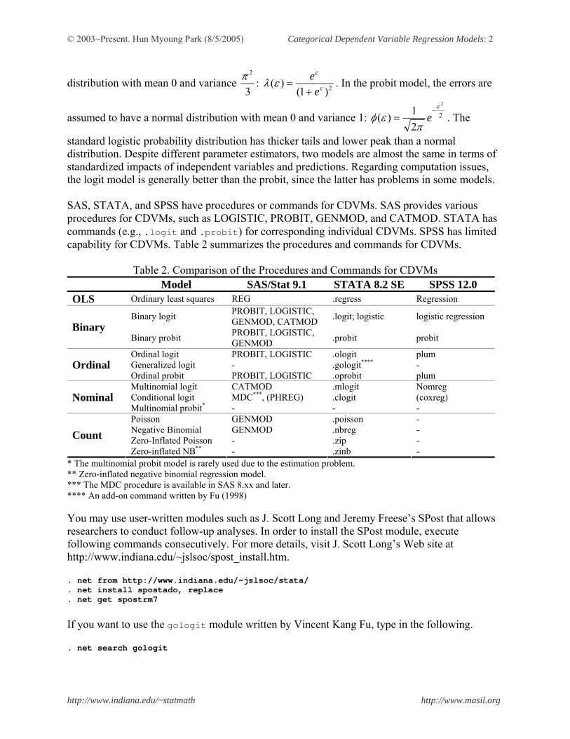
SAS, STATA, and SPSS have procedures or commands for CDVMs. SAS provides various procedures for CDVMs, such as LOGISTIC, PROBIT, GENMOD, and CATMOD. STATA has commands (e.g., .logit and .probit) for corresponding individual CDVMs. SPSS has limited capability for CDVMs. Table 2 summarizes the procedures and commands for CDVMs.
Table 2. Comparison of the Procedures and Commands for CDVMs
Model SAS/Stat 9.1 STATA 8.2 SE SPSS 12.0 OLS Ordinary least squares REG .regress Regression
Binary logit PROBIT, LOGISTIC, GENMOD, CATMOD .logit; logistic logistic regression
Binary Binary probit PROBIT, LOGISTIC,
GENMOD .probit probit
Ordinal logit PROBIT, LOGISTIC .ologit plum Generalized logit - .gologit**** - Ordinal Ordinal probit PROBIT, LOGISTIC .oprobit plum Multinomial logit CATMOD .mlogit Nomreg Conditional logit MDC***, (PHREG) .clogit (coxreg) Nominal Multinomial probit* - - - Poisson GENMOD .poisson - Negative Binomial GENMOD .nbreg - Zero-Inflated Poisson - .zip - Count Zero-inflated NB** - .zinb -
* The multinomial probit model is rarely used due to the estimation problem. ** Zero-inflated negative binomial regression model. *** The MDC procedure is available in SAS 8.xx and later. **** An add-on command written by Fu (1998) You may use user-written modules such as J. Scott Long and Jeremy Freese’s SPost that allows researchers to conduct follow-up analyses. In order to install the SPost module, execute following commands consecutively. For more details, visit J. Scott Long’s Web site at http://www.indiana.edu/~jslsoc/spost_install.htm. . net from http://www.indiana.edu/~jslsoc/stata/ . net install spostado, replace . net get spostrm7
If you want to use the gologit module written by Vincent Kang Fu, type in the following. . net search gologit
© 2003~Present. Hun Myoung Park (8/5/2005) Categorical Dependent Variable Regression Models: 3
http://www.indiana.edu/~statmath http://www.masil.org
2. Binary Logit Regression Model The binary logit model is represented as )(
)exp(1)exp()|1(Pr ββ
β xx
xxyob Λ=+
== , where Λ
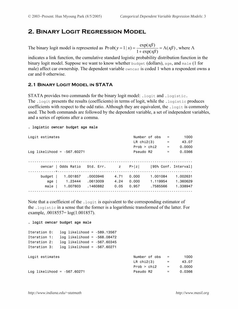
indicates a link function, the cumulative standard logistic probability distribution function in the binary logit model. Suppose we want to know whether budget (dollars), age, and male (1 for male) affect car ownership. The dependent variable owncar is coded 1 when a respondent owns a car and 0 otherwise.
2.1 Binary Logit Model in STATA STATA provides two commands for the binary logit model: .logit and .logistic. The .logit presents the results (coefficients) in terms of logit, while the .logistic produces coefficients with respect to the odd ratio. Although they are equivalent, the .logit is commonly used. The both commands are followed by the dependent variable, a set of independent variables, and a series of options after a comma. . logistic owncar budget age male Logit estimates Number of obs = 1000 LR chi2(3) = 43.07 Prob > chi2 = 0.0000 Log likelihood = -567.60271 Pseudo R2 = 0.0366 ------------------------------------------------------------------------------ owncar | Odds Ratio Std. Err. z P>|z| [95% Conf. Interval] -------------+---------------------------------------------------------------- budget | 1.001857 .0003946 4.71 0.000 1.001084 1.002631 age | 1.23444 .0613009 4.24 0.000 1.119954 1.360629 male | 1.007803 .1460882 0.05 0.957 .7585566 1.338947 ------------------------------------------------------------------------------ Note that a coeffieicnt of the .logit is equivalent to the corresponding estimator of the .logistic in a sense that the former is a logarithmic transformed of the latter. For example, .0018557= log(1.001857). . logit owncar budget age male Iteration 0: log likelihood = -589.13567 Iteration 1: log likelihood = -568.08472 Iteration 2: log likelihood = -567.60345 Iteration 3: log likelihood = -567.60271 Logit estimates Number of obs = 1000 LR chi2(3) = 43.07 Prob > chi2 = 0.0000 Log likelihood = -567.60271 Pseudo R2 = 0.0366

© 2003~Present. Hun Myoung Park (8/5/2005) Categorical Dependent Variable Regression Models: 4
http://www.indiana.edu/~statmath http://www.masil.org
------------------------------------------------------------------------------ owncar | Coef. Std. Err. z P>|z| [95% Conf. Interval] -------------+---------------------------------------------------------------- budget | .0018557 .0003939 4.71 0.000 .0010837 .0026277 age | .2106171 .0496589 4.24 0.000 .1132875 .3079467 male | .0077728 .1449571 0.05 0.957 -.2763379 .2918836 _cons | -4.567904 1.064209 -4.29 0.000 -6.653715 -2.482093 ------------------------------------------------------------------------------ Stata has post-estimation-commands that conduct follow-up analyses. For example, the .predict returns predictions and residuals, the .listcoef lists transformed coefficients (e.g., factor change in odds in binary logit model), the .fitstat shows goodness of fit measures. The .test and .lrtest respectively conduct Wald test and likelihood ratio test. . predict r, residuals . listcoef logit (N=1000): Factor Change in Odds Odds of: 1 vs 0 ---------------------------------------------------------------------- owncar | b z P>|z| e^b e^bStdX SDofX -------------+-------------------------------------------------------- budget | 0.00186 4.711 0.000 1.0019 1.4544 201.8442 age | 0.21062 4.241 0.000 1.2344 1.3992 1.5947 male | 0.00777 0.054 0.957 1.0078 1.0039 0.4986 ---------------------------------------------------------------------- . fitstat Measures of Fit for logit of owncar Log-Lik Intercept Only: -589.136 Log-Lik Full Model: -567.603 D(996): 1135.205 LR(3): 43.066 Prob > LR: 0.000 McFadden's R2: 0.037 McFadden's Adj R2: 0.030 Maximum Likelihood R2: 0.042 Cragg & Uhler's R2: 0.061 McKelvey and Zavoina's R2: 0.073 Efron's R2: 0.042 Variance of y*: 3.548 Variance of error: 3.290 Count R2: 0.727 Adj Count R2: 0.011 AIC: 1.143 AIC*n: 1143.205 BIC: -5744.919 BIC': -22.343 . test budget=male=0 ( 1) budget - male = 0 ( 2) budget = 0
© 2003~Present. Hun Myoung Park (8/5/2005) Categorical Dependent Variable Regression Models: 5
http://www.indiana.edu/~statmath http://www.masil.org
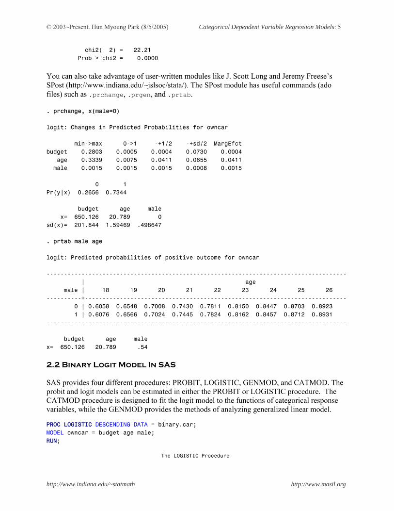
chi2( 2) = 22.21 Prob > chi2 = 0.0000 You can also take advantage of user-written modules like J. Scott Long and Jeremy Freese’s SPost (http://www.indiana.edu/~jslsoc/stata/). The SPost module has useful commands (ado files) such as .prchange, .prgen, and .prtab. . prchange, x(male=0) logit: Changes in Predicted Probabilities for owncar min->max 0->1 -+1/2 -+sd/2 MargEfct budget 0.2803 0.0005 0.0004 0.0730 0.0004 age 0.3339 0.0075 0.0411 0.0655 0.0411 male 0.0015 0.0015 0.0015 0.0008 0.0015 0 1 Pr(y|x) 0.2656 0.7344 budget age male x= 650.126 20.789 0 sd(x)= 201.844 1.59469 .498647 . prtab male age logit: Predicted probabilities of positive outcome for owncar -------------------------------------------------------------------------------------- | age male | 18 19 20 21 22 23 24 25 26 ----------+--------------------------------------------------------------------------- 0 | 0.6058 0.6548 0.7008 0.7430 0.7811 0.8150 0.8447 0.8703 0.8923 1 | 0.6076 0.6566 0.7024 0.7445 0.7824 0.8162 0.8457 0.8712 0.8931 -------------------------------------------------------------------------------------- budget age male x= 650.126 20.789 .54 2.2 Binary Logit Model In SAS SAS provides four different procedures: PROBIT, LOGISTIC, GENMOD, and CATMOD. The probit and logit models can be estimated in either the PROBIT or LOGISTIC procedure. The CATMOD procedure is designed to fit the logit model to the functions of categorical response variables, while the GENMOD provides the methods of analyzing generalized linear model. PROC LOGISTIC DESCENDING DATA = binary.car; MODEL owncar = budget age male; RUN; The LOGISTIC Procedure

© 2003~Present. Hun Myoung Park (8/5/2005) Categorical Dependent Variable Regression Models: 6
http://www.indiana.edu/~statmath http://www.masil.org
Model Information Data Set BINARY.CAR Response Variable owncar owncar Number of Response Levels 2 Number of Observations 1000 Model binary logit Optimization Technique Fisher's scoring Response Profile Ordered Total Value owncar Frequency 1 1 724 2 0 276 Probability modeled is owncar=1. Model Convergence Status Convergence criterion (GCONV=1E-8) satisfied. Model Fit Statistics Intercept Intercept and Criterion Only Covariates AIC 1180.271 1143.205 SC 1185.179 1162.836 -2 Log L 1178.271 1135.205 Testing Global Null Hypothesis: BETA=0 Test Chi-Square DF Pr > ChiSq Likelihood Ratio 43.0659 3 <.0001 Score 39.7773 3 <.0001 Wald 38.4868 3 <.0001 Analysis of Maximum Likelihood Estimates Standard Wald Parameter DF Estimate Error Chi-Square Pr > ChiSq Intercept 1 -4.5679 1.0642 18.4235 <.0001 budget 1 0.00186 0.000394 22.1965 <.0001 age 1 0.2106 0.0497 17.9881 <.0001 male 1 0.00777 0.1450 0.0029 0.9572 Odds Ratio Estimates

© 2003~Present. Hun Myoung Park (8/5/2005) Categorical Dependent Variable Regression Models: 7
http://www.indiana.edu/~statmath http://www.masil.org
Point 95% Wald Effect Estimate Confidence Limits budget 1.002 1.001 1.003 age 1.234 1.120 1.361 male 1.008 0.759 1.339 Association of Predicted Probabilities and Observed Responses Percent Concordant 63.0 Somers' D 0.266 Percent Discordant 36.4 Gamma 0.268 Percent Tied 0.7 Tau-a 0.106 Pairs 199824 c 0.633
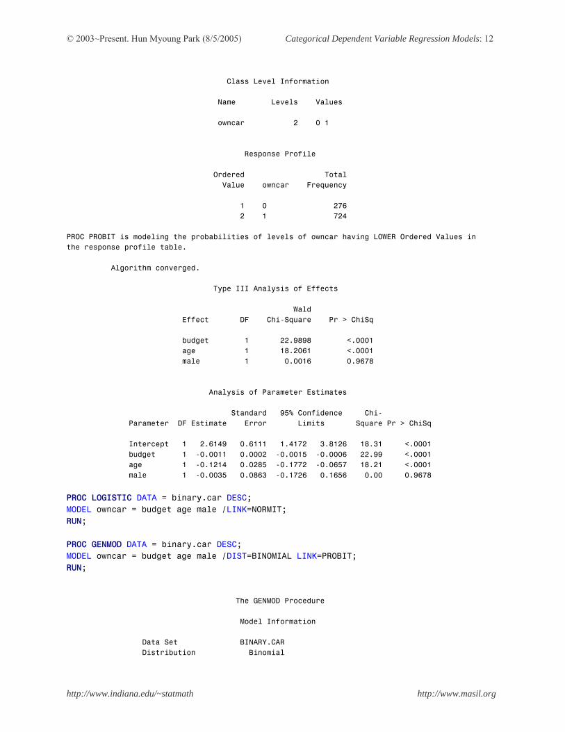
Note that the DESCENDING option forces SAS to use a larger value (e.g., 1) in the dependent variable as success. Otherwise, the coefficients have opposite signs to those of STATA and SPSS. PROC PROBIT DATA = binary.car; CLASS owncar; MODEL owncar = budget age male /DIST=LOGISTIC; RUN; Probit Procedure Model Information Data Set BINARY.CAR Dependent Variable owncar owncar Number of Observations 1000 Name of Distribution Logistic Log Likelihood -567.6027102 Class Level Information Name Levels Values owncar 2 0 1 Response Profile Ordered Total Value owncar Frequency 1 0 276 2 1 724 PROC PROBIT is modeling the probabilities of levels of owncar having LOWER Ordered Values in the response profile table. Algorithm converged.

© 2003~Present. Hun Myoung Park (8/5/2005) Categorical Dependent Variable Regression Models: 8
http://www.indiana.edu/~statmath http://www.masil.org
Type III Analysis of Effects Wald Effect DF Chi-Square Pr > ChiSq budget 1 22.1969 <.0001 age 1 17.9884 <.0001 male 1 0.0029 0.9572 Analysis of Parameter Estimates Standard 95% Confidence Chi- Parameter DF Estimate Error Limits Square Pr > ChiSq Intercept 1 4.5679 1.0642 2.4821 6.6537 18.42 <.0001 budget 1 -0.0019 0.0004 -0.0026 -0.0011 22.20 <.0001 age 1 -0.2106 0.0497 -0.3079 -0.1133 17.99 <.0001 male 1 -0.0078 0.1450 -0.2919 0.2763 0.00 0.9572 Unlike the LOGISTIC, the PROBIT does not have the DESCENDING option. It requires categorical variables to be explicitly specified in the CLASS statement. Note that the /DIST=LOGISTIC option specifies the probability distribution to be used in maximum likelihood estimation. The GENMOD procedure provides higher flexibility than other procedures. For instance, the procedure allows users to use categorical variables in the right-hand side without creating dummy variables (see the second example). The following two procedures return equivalent results. PROC GENMOD DATA = binary.car DESC; MODEL owncar = budget age male /DIST=BINOMIAL LINK=LOGIT; RUN; The GENMOD Procedure Model Information Data Set BINARY.CAR Distribution Binomial Link Function Logit Dependent Variable owncar owncar Observations Used 1000 Response Profile Ordered Total Value owncar Frequency 1 1 724 2 0 276 PROC GENMOD is modeling the probability that owncar='1'.

© 2003~Present. Hun Myoung Park (8/5/2005) Categorical Dependent Variable Regression Models: 9
http://www.indiana.edu/~statmath http://www.masil.org
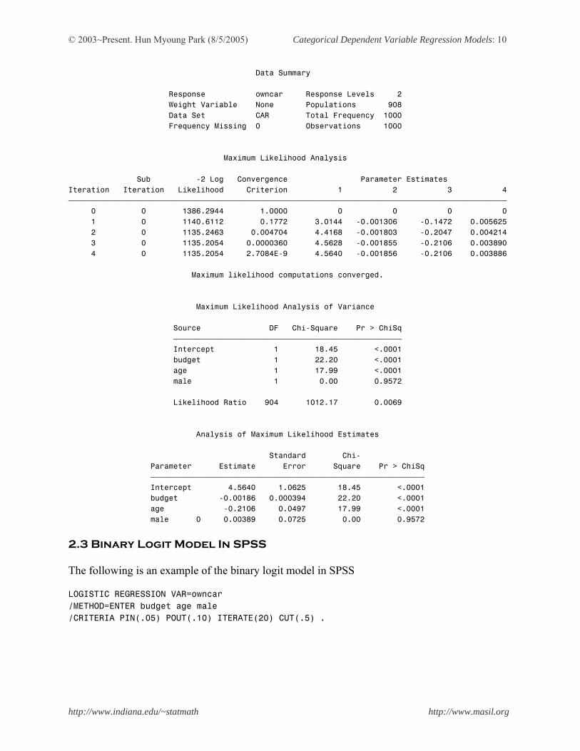
Criteria For Assessing Goodness Of Fit Criterion DF Value Value/DF Deviance 996 1135.2054 1.1398 Scaled Deviance 996 1135.2054 1.1398 Pearson Chi-Square 996 1004.3105 1.0083 Scaled Pearson X2 996 1004.3105 1.0083 Log Likelihood -567.6027 Algorithm converged. Analysis Of Parameter Estimates Standard Wald 95% Confidence Chi- Parameter DF Estimate Error Limits Square Pr > ChiSq Intercept 1 -4.5679 1.0642 -6.6537 -2.4821 18.42 <.0001 budget 1 0.0019 0.0004 0.0011 0.0026 22.20 <.0001 age 1 0.2106 0.0497 0.1133 0.3079 17.99 <.0001 male 1 0.0078 0.1450 -0.2763 0.2919 0.00 0.9572 Scale 0 1.0000 0.0000 1.0000 1.0000 NOTE: The scale parameter was held fixed. PROC GENMOD DATA = binary.car DESC; CLASS male; MODEL owncar = budget age male /DIST=BINOMIAL LINK=LOGIT; RUN; Note that the LINK=LOGIT option specifies the link function. Alternatively, you may write explicitly the link function using the FWDLINK and INVLINK statements instead of the LINK=LOGIT option. This method produces the identical result to the above output. PROC GENMOD DATA = binary.car DESC; FWDLINK link=LOG(_MEAN_/(1-_MEAN_)); INVLINK invlink=1/(1+EXP(-1*_XBETA_)); MODEL owncar = budget age male /DIST=BINOMIAL; RUN; The following example uses the CATMOD procedure, which produces slightly different estimators. So, this procedure is less recommended for the binary logit model. Interval or ratio variables should be specified in the DIRECT statement. Note that the /NOPROFILE suppresses the display of the population profiles and the response profiles. PROC CATMOD DATA = binary.car; DIRECT budget age; MODEL owncar = budget age male /NOPROFILE; RUN; The CATMOD Procedure
© 2003~Present. Hun Myoung Park (8/5/2005) Categorical Dependent Variable Regression Models: 10
http://www.indiana.edu/~statmath http://www.masil.org
Data Summary Response owncar Response Levels 2 Weight Variable None Populations 908 Data Set CAR Total Frequency 1000 Frequency Missing 0 Observations 1000 Maximum Likelihood Analysis Sub -2 Log Convergence Parameter Estimates Iteration Iteration Likelihood Criterion 1 2 3 4 ƒƒƒƒƒƒƒƒƒƒƒƒƒƒƒƒƒƒƒƒƒƒƒƒƒƒƒƒƒƒƒƒƒƒƒƒƒƒƒƒƒƒƒƒƒƒƒƒƒƒƒƒƒƒƒƒƒƒƒƒƒƒƒƒƒƒƒƒƒƒƒƒƒƒƒƒƒƒƒƒƒƒƒƒƒƒƒƒƒƒƒƒƒƒƒƒ 0 0 1386.2944 1.0000 0 0 0 0 1 0 1140.6112 0.1772 3.0144 -0.001306 -0.1472 0.005625 2 0 1135.2463 0.004704 4.4168 -0.001803 -0.2047 0.004214 3 0 1135.2054 0.0000360 4.5628 -0.001855 -0.2106 0.003890 4 0 1135.2054 2.7084E-9 4.5640 -0.001856 -0.2106 0.003886 Maximum likelihood computations converged. Maximum Likelihood Analysis of Variance Source DF Chi-Square Pr > ChiSq ƒƒƒƒƒƒƒƒƒƒƒƒƒƒƒƒƒƒƒƒƒƒƒƒƒƒƒƒƒƒƒƒƒƒƒƒƒƒƒƒƒƒƒƒƒƒƒƒƒƒ Intercept 1 18.45 <.0001 budget 1 22.20 <.0001 age 1 17.99 <.0001 male 1 0.00 0.9572 Likelihood Ratio 904 1012.17 0.0069 Analysis of Maximum Likelihood Estimates Standard Chi- Parameter Estimate Error Square Pr > ChiSq ƒƒƒƒƒƒƒƒƒƒƒƒƒƒƒƒƒƒƒƒƒƒƒƒƒƒƒƒƒƒƒƒƒƒƒƒƒƒƒƒƒƒƒƒƒƒƒƒƒƒƒƒƒƒƒƒƒƒƒƒ Intercept 4.5640 1.0625 18.45 <.0001 budget -0.00186 0.000394 22.20 <.0001 age -0.2106 0.0497 17.99 <.0001 male 0 0.00389 0.0725 0.00 0.9572
2.3 Binary Logit Model In SPSS The following is an example of the binary logit model in SPSS LOGISTIC REGRESSION VAR=owncar /METHOD=ENTER budget age male /CRITERIA PIN(.05) POUT(.10) ITERATE(20) CUT(.5) .

© 2003~Present. Hun Myoung Park (8/5/2005) Categorical Dependent Variable Regression Models: 11
http://www.indiana.edu/~statmath http://www.masil.org
3. Binary Probit Regression Model The probit model is represented as )()|1(Pr βxxyob Φ== , where Φ indicates the cumulative normal distribution function. 3.1 Binary Probit In STATA STATA has the .probit command with the similar usage as .logit. . probit owncar budget age male Iteration 0: log likelihood = -589.13567 Iteration 1: log likelihood = -567.89453 Iteration 2: log likelihood = -567.71705 Iteration 3: log likelihood = -567.71702 Probit estimates Number of obs = 1000 LR chi2(3) = 42.84 Prob > chi2 = 0.0000 Log likelihood = -567.71702 Pseudo R2 = 0.0364 ------------------------------------------------------------------------------ owncar | Coef. Std. Err. z P>|z| [95% Conf. Interval] -------------+---------------------------------------------------------------- budget | .001092 .0002277 4.79 0.000 .0006456 .0015384 age | .1214482 .0284631 4.27 0.000 .0656614 .1772349 male | .0034862 .0862954 0.04 0.968 -.1656498 .1726221 _cons | -2.614903 .6110651 -4.28 0.000 -3.812568 -1.417237 ------------------------------------------------------------------------------ 3.2 Binary Probit In SAS You can use the PROBIT, the LOGISTIC, or GENMOD procedure to estimate the binary probit model. Keep in mind that the coefficients of the PROBIT has opposite signs. PROC PROBIT DATA = binary.car; CLASS owncar; MODEL owncar = budget age male; RUN; Probit Procedure Model Information Data Set BINARY.CAR Dependent Variable owncar owncar Number of Observations 1000 Name of Distribution Normal Log Likelihood -567.7170164
© 2003~Present. Hun Myoung Park (8/5/2005) Categorical Dependent Variable Regression Models: 12
http://www.indiana.edu/~statmath http://www.masil.org
Class Level Information Name Levels Values owncar 2 0 1 Response Profile Ordered Total Value owncar Frequency 1 0 276 2 1 724 PROC PROBIT is modeling the probabilities of levels of owncar having LOWER Ordered Values in the response profile table. Algorithm converged. Type III Analysis of Effects Wald Effect DF Chi-Square Pr > ChiSq budget 1 22.9898 <.0001 age 1 18.2061 <.0001 male 1 0.0016 0.9678 Analysis of Parameter Estimates Standard 95% Confidence Chi- Parameter DF Estimate Error Limits Square Pr > ChiSq Intercept 1 2.6149 0.6111 1.4172 3.8126 18.31 <.0001 budget 1 -0.0011 0.0002 -0.0015 -0.0006 22.99 <.0001 age 1 -0.1214 0.0285 -0.1772 -0.0657 18.21 <.0001 male 1 -0.0035 0.0863 -0.1726 0.1656 0.00 0.9678 PROC LOGISTIC DATA = binary.car DESC; MODEL owncar = budget age male /LINK=NORMIT; RUN; PROC GENMOD DATA = binary.car DESC; MODEL owncar = budget age male /DIST=BINOMIAL LINK=PROBIT; RUN; The GENMOD Procedure Model Information Data Set BINARY.CAR Distribution Binomial

© 2003~Present. Hun Myoung Park (8/5/2005) Categorical Dependent Variable Regression Models: 13
http://www.indiana.edu/~statmath http://www.masil.org
Link Function Probit Dependent Variable owncar owncar Observations Used 1000 Response Profile Ordered Total Value owncar Frequency 1 1 724 2 0 276 PROC GENMOD is modeling the probability that owncar='1'. Criteria For Assessing Goodness Of Fit Criterion DF Value Value/DF Deviance 996 1135.4340 1.1400 Scaled Deviance 996 1135.4340 1.1400 Pearson Chi-Square 996 1007.4937 1.0115 Scaled Pearson X2 996 1007.4937 1.0115 Log Likelihood -567.7170 Algorithm converged. Analysis Of Parameter Estimates Standard Wald 95% Confidence Chi- Parameter DF Estimate Error Limits Square Pr > ChiSq Intercept 1 -2.6149 0.6111 -3.8126 -1.4172 18.31 <.0001 budget 1 0.0011 0.0002 0.0006 0.0015 22.99 <.0001 age 1 0.1214 0.0285 0.0657 0.1772 18.21 <.0001 male 1 0.0035 0.0863 -0.1656 0.1726 0.00 0.9678 Scale 0 1.0000 0.0000 1.0000 1.0000 NOTE: The scale parameter was held fixed. Note that /LINK=NORMIT or /LINK=PROBIT in the PROC LOGISTIC indicate the normal probability distribution, while the /LINK=PROBIT in the PROC GENMOD specifies PROBIT as the link function. 3.3 Binary Probit In SPSS The following is an example of the binary probit in SPSS. Note that the variable n with constant 1 is created to be used in the probit command. COMPUTE n=1. PROBIT owncar OF n WITH budget age sex /LOG NONE /MODEL PROBIT /PRINT FREQ /CRITERIA ITERATE(20) STEPLIMIT(.1).
© 2003~Present. Hun Myoung Park (8/5/2005) Categorical Dependent Variable Regression Models: 14
http://www.indiana.edu/~statmath http://www.masil.org
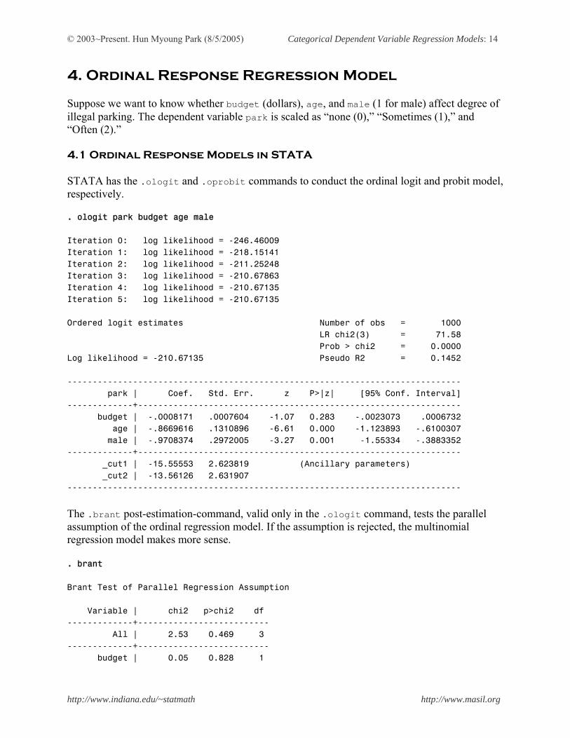
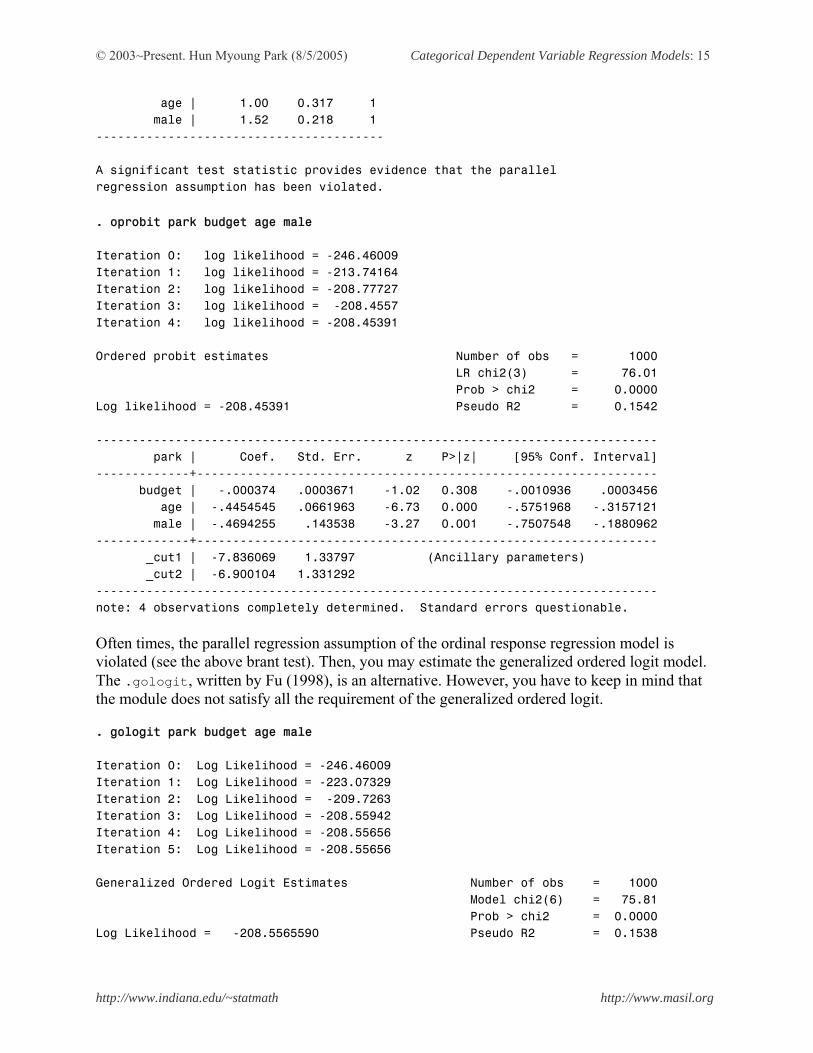
4. Ordinal Response Regression Model Suppose we want to know whether budget (dollars), age, and male (1 for male) affect degree of illegal parking. The dependent variable park is scaled as “none (0),” “Sometimes (1),” and “Often (2).” 4.1 Ordinal Response Models in STATA STATA has the .ologit and .oprobit commands to conduct the ordinal logit and probit model, respectively. . ologit park budget age male Iteration 0: log likelihood = -246.46009 Iteration 1: log likelihood = -218.15141 Iteration 2: log likelihood = -211.25248 Iteration 3: log likelihood = -210.67863 Iteration 4: log likelihood = -210.67135 Iteration 5: log likelihood = -210.67135 Ordered logit estimates Number of obs = 1000 LR chi2(3) = 71.58 Prob > chi2 = 0.0000 Log likelihood = -210.67135 Pseudo R2 = 0.1452 ------------------------------------------------------------------------------ park | Coef. Std. Err. z P>|z| [95% Conf. Interval] -------------+---------------------------------------------------------------- budget | -.0008171 .0007604 -1.07 0.283 -.0023073 .0006732 age | -.8669616 .1310896 -6.61 0.000 -1.123893 -.6100307 male | -.9708374 .2972005 -3.27 0.001 -1.55334 -.3883352 -------------+---------------------------------------------------------------- _cut1 | -15.55553 2.623819 (Ancillary parameters) _cut2 | -13.56126 2.631907 ------------------------------------------------------------------------------ The .brant post-estimation-command, valid only in the .ologit command, tests the parallel assumption of the ordinal regression model. If the assumption is rejected, the multinomial regression model makes more sense. . brant Brant Test of Parallel Regression Assumption Variable | chi2 p>chi2 df -------------+-------------------------- All | 2.53 0.469 3 -------------+-------------------------- budget | 0.05 0.828 1
© 2003~Present. Hun Myoung Park (8/5/2005) Categorical Dependent Variable Regression Models: 15
http://www.indiana.edu/~statmath http://www.masil.org
age | 1.00 0.317 1 male | 1.52 0.218 1 ---------------------------------------- A significant test statistic provides evidence that the parallel regression assumption has been violated. . oprobit park budget age male Iteration 0: log likelihood = -246.46009 Iteration 1: log likelihood = -213.74164 Iteration 2: log likelihood = -208.77727 Iteration 3: log likelihood = -208.4557 Iteration 4: log likelihood = -208.45391 Ordered probit estimates Number of obs = 1000 LR chi2(3) = 76.01 Prob > chi2 = 0.0000 Log likelihood = -208.45391 Pseudo R2 = 0.1542 ------------------------------------------------------------------------------ park | Coef. Std. Err. z P>|z| [95% Conf. Interval] -------------+---------------------------------------------------------------- budget | -.000374 .0003671 -1.02 0.308 -.0010936 .0003456 age | -.4454545 .0661963 -6.73 0.000 -.5751968 -.3157121 male | -.4694255 .143538 -3.27 0.001 -.7507548 -.1880962 -------------+---------------------------------------------------------------- _cut1 | -7.836069 1.33797 (Ancillary parameters) _cut2 | -6.900104 1.331292 ------------------------------------------------------------------------------ note: 4 observations completely determined. Standard errors questionable. Often times, the parallel regression assumption of the ordinal response regression model is violated (see the above brant test). Then, you may estimate the generalized ordered logit model. The .gologit, written by Fu (1998), is an alternative. However, you have to keep in mind that the module does not satisfy all the requirement of the generalized ordered logit. . gologit park budget age male Iteration 0: Log Likelihood = -246.46009 Iteration 1: Log Likelihood = -223.07329 Iteration 2: Log Likelihood = -209.7263 Iteration 3: Log Likelihood = -208.55942 Iteration 4: Log Likelihood = -208.55656 Iteration 5: Log Likelihood = -208.55656 Generalized Ordered Logit Estimates Number of obs = 1000 Model chi2(6) = 75.81 Prob > chi2 = 0.0000 Log Likelihood = -208.5565590 Pseudo R2 = 0.1538
© 2003~Present. Hun Myoung Park (8/5/2005) Categorical Dependent Variable Regression Models: 16
http://www.indiana.edu/~statmath http://www.masil.org
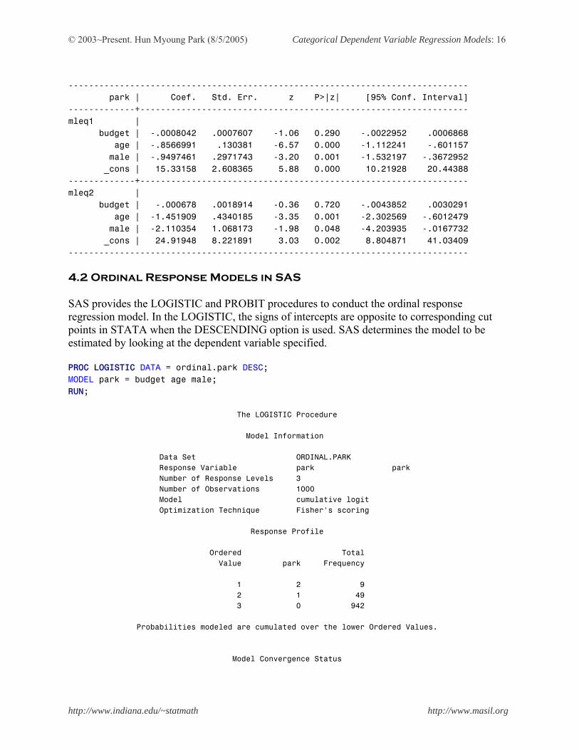
------------------------------------------------------------------------------ park | Coef. Std. Err. z P>|z| [95% Conf. Interval] -------------+---------------------------------------------------------------- mleq1 | budget | -.0008042 .0007607 -1.06 0.290 -.0022952 .0006868 age | -.8566991 .130381 -6.57 0.000 -1.112241 -.601157 male | -.9497461 .2971743 -3.20 0.001 -1.532197 -.3672952 _cons | 15.33158 2.608365 5.88 0.000 10.21928 20.44388 -------------+---------------------------------------------------------------- mleq2 | budget | -.000678 .0018914 -0.36 0.720 -.0043852 .0030291 age | -1.451909 .4340185 -3.35 0.001 -2.302569 -.6012479 male | -2.110354 1.068173 -1.98 0.048 -4.203935 -.0167732 _cons | 24.91948 8.221891 3.03 0.002 8.804871 41.03409 ------------------------------------------------------------------------------ 4.2 Ordinal Response Models in SAS SAS provides the LOGISTIC and PROBIT procedures to conduct the ordinal response regression model. In the LOGISTIC, the signs of intercepts are opposite to corresponding cut points in STATA when the DESCENDING option is used. SAS determines the model to be estimated by looking at the dependent variable specified. PROC LOGISTIC DATA = ordinal.park DESC; MODEL park = budget age male; RUN; The LOGISTIC Procedure Model Information Data Set ORDINAL.PARK Response Variable park park Number of Response Levels 3 Number of Observations 1000 Model cumulative logit Optimization Technique Fisher's scoring Response Profile Ordered Total Value park Frequency 1 2 9 2 1 49 3 0 942 Probabilities modeled are cumulated over the lower Ordered Values. Model Convergence Status
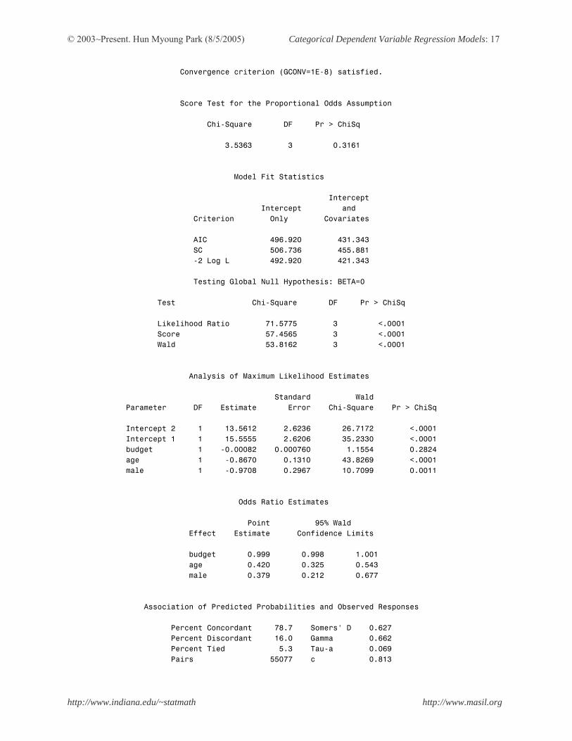
© 2003~Present. Hun Myoung Park (8/5/2005) Categorical Dependent Variable Regression Models: 17
http://www.indiana.edu/~statmath http://www.masil.org
Convergence criterion (GCONV=1E-8) satisfied. Score Test for the Proportional Odds Assumption Chi-Square DF Pr > ChiSq 3.5363 3 0.3161 Model Fit Statistics Intercept Intercept and Criterion Only Covariates AIC 496.920 431.343 SC 506.736 455.881 -2 Log L 492.920 421.343 Testing Global Null Hypothesis: BETA=0 Test Chi-Square DF Pr > ChiSq Likelihood Ratio 71.5775 3 <.0001 Score 57.4565 3 <.0001 Wald 53.8162 3 <.0001 Analysis of Maximum Likelihood Estimates Standard Wald Parameter DF Estimate Error Chi-Square Pr > ChiSq Intercept 2 1 13.5612 2.6236 26.7172 <.0001 Intercept 1 1 15.5555 2.6206 35.2330 <.0001 budget 1 -0.00082 0.000760 1.1554 0.2824 age 1 -0.8670 0.1310 43.8269 <.0001 male 1 -0.9708 0.2967 10.7099 0.0011 Odds Ratio Estimates Point 95% Wald Effect Estimate Confidence Limits budget 0.999 0.998 1.001 age 0.420 0.325 0.543 male 0.379 0.212 0.677 Association of Predicted Probabilities and Observed Responses Percent Concordant 78.7 Somers' D 0.627 Percent Discordant 16.0 Gamma 0.662 Percent Tied 5.3 Tau-a 0.069 Pairs 55077 c 0.813
© 2003~Present. Hun Myoung Park (8/5/2005) Categorical Dependent Variable Regression Models: 18
http://www.indiana.edu/~statmath http://www.masil.org
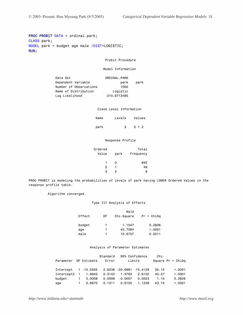
PROC PROBIT DATA = ordinal.park; CLASS park; MODEL park = budget age male /DIST=LOGISTIC; RUN; Probit Procedure Model Information Data Set ORDINAL.PARK Dependent Variable park park Number of Observations 1000 Name of Distribution Logistic Log Likelihood -210.6713485 Class Level Information Name Levels Values park 3 0 1 2 Response Profile Ordered Total Value park Frequency 1 0 942 2 1 49 3 2 9 PROC PROBIT is modeling the probabilities of levels of park having LOWER Ordered Values in the response profile table. Algorithm converged. Type III Analysis of Effects Wald Effect DF Chi-Square Pr > ChiSq budget 1 1.1547 0.2826 age 1 43.7384 <.0001 male 1 10.6707 0.0011 Analysis of Parameter Estimates Standard 95% Confidence Chi- Parameter DF Estimate Error Limits Square Pr > ChiSq Intercept 1 -15.5555 2.6238 -20.6981 -10.4129 35.15 <.0001 Intercept2 1 1.9943 0.3143 1.3783 2.6102 40.27 <.0001 budget 1 0.0008 0.0008 -0.0007 0.0023 1.15 0.2826 age 1 0.8670 0.1311 0.6100 1.1239 43.74 <.0001

© 2003~Present. Hun Myoung Park (8/5/2005) Categorical Dependent Variable Regression Models: 19
http://www.indiana.edu/~statmath http://www.masil.org
male 1 0.9708 0.2972 0.3883 1.5533 10.67 0.0011
Keep in mind that the signs of coefficients are opposite in the PROBIT procedure. The following two procedures estimate the ordinal probit model. PROC PROBIT DATA = ordinal.park; CLASS park; MODEL park = budget age male /DIST=NORMAL; RUN; Probit Procedure Model Information Data Set ORDINAL.PARK Dependent Variable park park Number of Observations 1000 Name of Distribution Normal Log Likelihood -208.4539066 Class Level Information Name Levels Values park 3 0 1 2 Response Profile Ordered Total Value park Frequency 1 0 942 2 1 49 3 2 9 PROC PROBIT is modeling the probabilities of levels of park having LOWER Ordered Values in the response profile table. Algorithm converged. Type III Analysis of Effects Wald Effect DF Chi-Square Pr > ChiSq budget 1 1.0378 0.3083 age 1 45.2810 <.0001 male 1 10.6952 0.0011 Analysis of Parameter Estimates

© 2003~Present. Hun Myoung Park (8/5/2005) Categorical Dependent Variable Regression Models: 20
http://www.indiana.edu/~statmath http://www.masil.org
Standard 95% Confidence Chi- Parameter DF Estimate Error Limits Square Pr > ChiSq Intercept 1 -7.8361 1.3380 -10.4585 -5.2136 34.30 <.0001 Intercept2 1 0.9360 0.1337 0.6739 1.1981 48.99 <.0001 budget 1 0.0004 0.0004 -0.0003 0.0011 1.04 0.3083 age 1 0.4455 0.0662 0.3157 0.5752 45.28 <.0001 male 1 0.4694 0.1435 0.1881 0.7508 10.70 0.0011
PROC LOGISTIC DATA = ordinal.park DESC; MODEL park = budget age male /LINK=NORMIT; RUN;
4.3 Ordinal Response Models in SPSS The followings are the examples of ordinal logit and probit models in SPSS. PLUM park WITH budget age male /CRITERIA = CIN(95) DELTA(0) LCONVERGE(0) MXITER(100) MXSTEP(5) PCONVERGE(1.0E-6) SINGULAR(1.0E-8) /LINK = LOGIT /PRINT = FIT PARAMETER SUMMARY . PLUM park WITH budget age male /CRITERIA = CIN(95) DELTA(0) LCONVERGE(0) MXITER(100) MXSTEP(5) PCONVERGE(1.0E-6) SINGULAR(1.0E-8) /LINK = PROBIT /PRINT = FIT PARAMETER SUMMARY .

© 2003~Present. Hun Myoung Park (8/5/2005) Categorical Dependent Variable Regression Models: 21
http://www.indiana.edu/~statmath http://www.masil.org
5. Nominal Response Regression Model Suppose we want to know how budget, age, and male affect the modes of transportation (walk, bike, bus, and car). The multinomial logit and conditional logit models are commonly used; the multinomial probit model is rarely used mainly due to the practical difficulty in estimation. In the multinomial logit model, the independent variables contain characteristics of individuals, while they are the attributes of the choices in the conditional logit model. In other words, the conditional logit estimates how alternative-specifit, not individual-specific, variables affect the likelihood of observing a given outcome (Long 2001). Therefore, data need to be appropriately arranged in advance. 5.1 Multinomial Logit Model in STATA STATA has the .mlogit for the multinomial logit model. In the following example, the “base(3)” option indicates the value to be used as the base of the estimation. The default is zero, “walk” in this example.
. mlogit mode budget age male, base(3) Iteration 0: log likelihood = -1308.7916 Iteration 1: log likelihood = -1171.4576 Iteration 2: log likelihood = -1162.1648 Iteration 3: log likelihood = -1162.0211 Iteration 4: log likelihood = -1162.021 Multinomial regression Number of obs = 1000 LR chi2(9) = 293.54 Prob > chi2 = 0.0000 Log likelihood = -1162.021 Pseudo R2 = 0.1121 ------------------------------------------------------------------------------ mode | Coef. Std. Err. z P>|z| [95% Conf. Interval] -------------+---------------------------------------------------------------- 0 | budget | -.0024153 .0005906 -4.09 0.000 -.0035729 -.0012577 age | -.0319581 .0555309 -0.58 0.565 -.1407966 .0768804 male | -.2436411 .1744193 -1.40 0.162 -.5854967 .0982145 _cons | 1.505895 1.211733 1.24 0.214 -.8690574 3.880848 -------------+---------------------------------------------------------------- 1 | budget | .0003189 .000588 0.54 0.588 -.0008336 .0014715 age | -.003483 .0630353 -0.06 0.956 -.1270299 .1200639 male | -.2463091 .2005415 -1.23 0.219 -.6393632 .1467449 _cons | -1.085158 1.371186 -0.79 0.429 -3.772633 1.602317 -------------+---------------------------------------------------------------- 2 | budget | .0060655 .0005117 11.85 0.000 .0050625 .0070685 age | -.0388937 .0581579 -0.67 0.504 -.1528811 .0750937

© 2003~Present. Hun Myoung Park (8/5/2005) Categorical Dependent Variable Regression Models: 22
http://www.indiana.edu/~statmath http://www.masil.org
male | -.8300401 .1849542 -4.49 0.000 -1.192544 -.4675366 _cons | -3.526573 1.255177 -2.81 0.005 -5.986675 -1.06647 ------------------------------------------------------------------------------ (Outcome mode==3 is the comparison group) 5.2 Multinomial Logit Model in SAS SAS has the CATMOD procedures for the multinomial logit. In the CATMOD procedure, the RESPONSE statement is used to specify the functions of response probabilities. PROC CATMOD DATA = nominal.trans; DIRECT budget age male; RESPONSE LOGITS; MODEL mode = budget age male /NOPROFILE; RUN; The CATMOD Procedure Data Summary Response mode Response Levels 4 Weight Variable None Populations 908 Data Set TRANS Total Frequency 1000 Frequency Missing 0 Observations 1000 Maximum Likelihood Analysis Sub -2 Log Convergence Parameter Estimates Iteration Iteration Likelihood Criterion 1 2 3 4 ƒƒƒƒƒƒƒƒƒƒƒƒƒƒƒƒƒƒƒƒƒƒƒƒƒƒƒƒƒƒƒƒƒƒƒƒƒƒƒƒƒƒƒƒƒƒƒƒƒƒƒƒƒƒƒƒƒƒƒƒƒƒƒƒƒƒƒƒƒƒƒƒƒƒƒƒƒƒƒƒƒƒƒƒƒƒƒƒƒƒƒƒƒƒƒƒ 0 0 2772.5887 1.0000 0 0 0 0 1 0 2347.3551 0.1534 0.1975 -1.3904 -3.4638 -0.000265 2 0 2324.2323 0.009851 1.5034 -1.0871 -3.4353 -0.002401 3 0 2324.042 0.0000819 1.5052 -1.0848 -3.5253 -0.002414 4 0 2324.042 1.1335E-8 1.5059 -1.0852 -3.5266 -0.002415 5 0 2324.042 2.152E-15 1.5059 -1.0852 -3.5266 -0.002415 Maximum Likelihood Analysis Parameter Estimates Iteration 5 6 7 8 9 10 11 ƒƒƒƒƒƒƒƒƒƒƒƒƒƒƒƒƒƒƒƒƒƒƒƒƒƒƒƒƒƒƒƒƒƒƒƒƒƒƒƒƒƒƒƒƒƒƒƒƒƒƒƒƒƒƒƒƒƒƒƒƒƒƒƒƒƒƒƒƒƒƒƒƒƒƒƒƒƒƒƒƒƒƒƒƒƒƒƒƒƒƒƒƒ 0 0 0 0 0 0 0 0 1 0.001300 0.006086 -0.0293 -0.0158 -0.0328 -0.4163 -0.3965 2 0.000285 0.005903 -0.0314 -0.002710 -0.0380 -0.2315 -0.2416 3 0.000319 0.006064 -0.0320 -0.003491 -0.0389 -0.2436 -0.2463 4 0.000319 0.006065 -0.0320 -0.003483 -0.0389 -0.2436 -0.2463 5 0.000319 0.006065 -0.0320 -0.003483 -0.0389 -0.2436 -0.2463 Maximum Likelihood Analysis Parameter Estimates
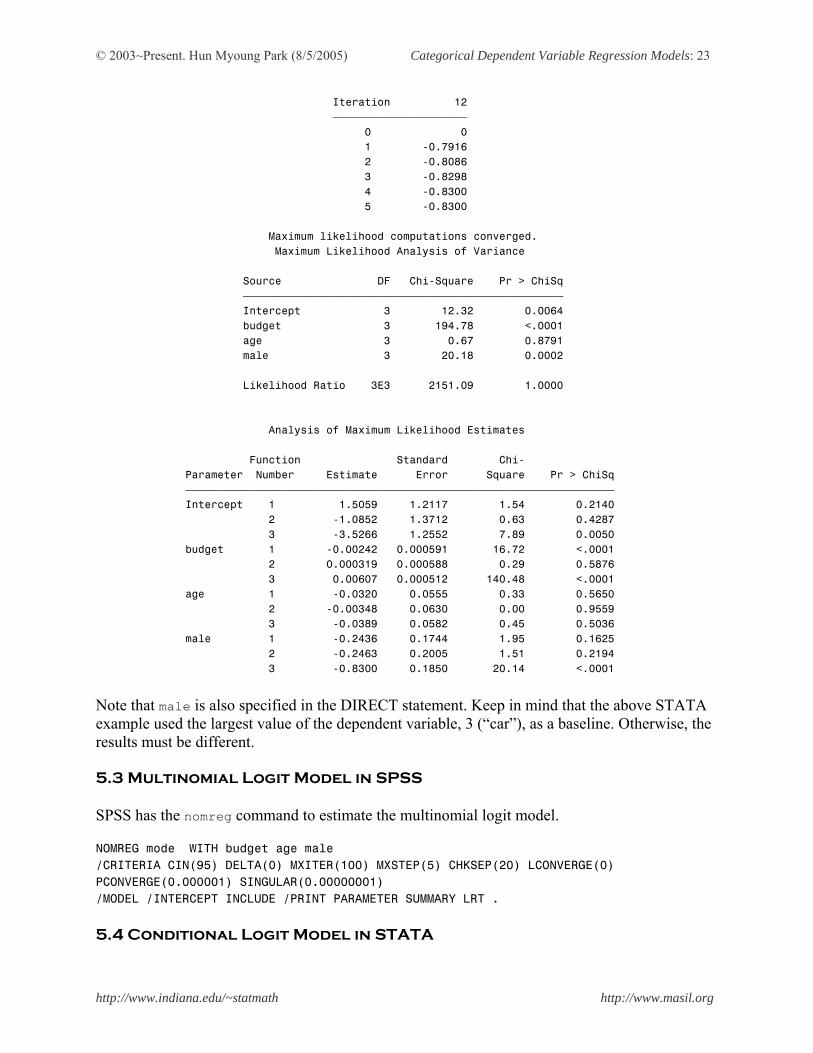
© 2003~Present. Hun Myoung Park (8/5/2005) Categorical Dependent Variable Regression Models: 23
http://www.indiana.edu/~statmath http://www.masil.org
Iteration 12 ƒƒƒƒƒƒƒƒƒƒƒƒƒƒƒƒƒƒƒƒƒ 0 0 1 -0.7916 2 -0.8086 3 -0.8298 4 -0.8300 5 -0.8300 Maximum likelihood computations converged. Maximum Likelihood Analysis of Variance Source DF Chi-Square Pr > ChiSq ƒƒƒƒƒƒƒƒƒƒƒƒƒƒƒƒƒƒƒƒƒƒƒƒƒƒƒƒƒƒƒƒƒƒƒƒƒƒƒƒƒƒƒƒƒƒƒƒƒƒ Intercept 3 12.32 0.0064 budget 3 194.78 <.0001 age 3 0.67 0.8791 male 3 20.18 0.0002 Likelihood Ratio 3E3 2151.09 1.0000 Analysis of Maximum Likelihood Estimates Function Standard Chi- Parameter Number Estimate Error Square Pr > ChiSq ƒƒƒƒƒƒƒƒƒƒƒƒƒƒƒƒƒƒƒƒƒƒƒƒƒƒƒƒƒƒƒƒƒƒƒƒƒƒƒƒƒƒƒƒƒƒƒƒƒƒƒƒƒƒƒƒƒƒƒƒƒƒƒƒƒƒƒ Intercept 1 1.5059 1.2117 1.54 0.2140 2 -1.0852 1.3712 0.63 0.4287 3 -3.5266 1.2552 7.89 0.0050 budget 1 -0.00242 0.000591 16.72 <.0001 2 0.000319 0.000588 0.29 0.5876 3 0.00607 0.000512 140.48 <.0001 age 1 -0.0320 0.0555 0.33 0.5650 2 -0.00348 0.0630 0.00 0.9559 3 -0.0389 0.0582 0.45 0.5036 male 1 -0.2436 0.1744 1.95 0.1625 2 -0.2463 0.2005 1.51 0.2194 3 -0.8300 0.1850 20.14 <.0001 Note that male is also specified in the DIRECT statement. Keep in mind that the above STATA example used the largest value of the dependent variable, 3 (“car”), as a baseline. Otherwise, the results must be different. 5.3 Multinomial Logit Model in SPSS SPSS has the nomreg command to estimate the multinomial logit model. NOMREG mode WITH budget age male /CRITERIA CIN(95) DELTA(0) MXITER(100) MXSTEP(5) CHKSEP(20) LCONVERGE(0) PCONVERGE(0.000001) SINGULAR(0.00000001) /MODEL /INTERCEPT INCLUDE /PRINT PARAMETER SUMMARY LRT . 5.4 Conditional Logit Model in STATA

© 2003~Present. Hun Myoung Park (8/5/2005) Categorical Dependent Variable Regression Models: 24
http://www.indiana.edu/~statmath http://www.masil.org
Suppose the choice of mode of transportation is affected by time (minutes) and cost (dollars) spent on the four alternatives of walk, bike, bus, and car. There are 210 subjects, each of whom has four choices; thus total 850 cases are included in the data set. The dependent variable is set 1 if the subject chooses the mode of transportation and zero otherwise. STATA has the .clogit command to estimate the condition logit model. Following is an example of the model. Note that walk, bike, and bus are dummy variables for flagging the mode of transportation. For example, the bus is set 1 if an observation contains information about taking a bus. The group() option specifies the variable that identify unique subjects. . clogit choice walk bike bus time cost, group(subject) Iteration 0: log likelihood = -262.77756 Iteration 1: log likelihood = -209.50653 Iteration 2: log likelihood = -205.72682 Iteration 3: log likelihood = -205.5967 Iteration 4: log likelihood = -205.59646 Conditional (fixed-effects) logistic regression Number of obs = 840 LR chi2(5) = 171.05 Prob > chi2 = 0.0000 Log likelihood = -205.59646 Pseudo R2 = 0.2938 ------------------------------------------------------------------------------ choice | Coef. Std. Err. z P>|z| [95% Conf. Interval] -------------+---------------------------------------------------------------- walk | 6.54371 .7815754 8.37 0.000 5.011851 8.07557 bike | 3.808292 .4600735 8.28 0.000 2.906564 4.710019 bus | 3.202466 .4537241 7.06 0.000 2.313183 4.091749 time | -.1000569 .0104929 -9.54 0.000 -.1206226 -.0794912 cost | -.0097447 .0062539 -1.56 0.119 -.0220022 .0025128 ------------------------------------------------------------------------------ . listcoef clogit (N=840): Factor Change in Odds Odds of: 1 vs 0 -------------------------------------------------- choice | b z P>|z| e^b -------------+------------------------------------ walk | 6.54371 8.372 0.000 694.8600 bike | 3.80829 8.278 0.000 45.0734 bus | 3.20247 7.058 0.000 24.5931 time | -0.10006 -9.536 0.000 0.9048 cost | -0.00974 -1.558 0.119 0.9903 --------------------------------------------------

© 2003~Present. Hun Myoung Park (8/5/2005) Categorical Dependent Variable Regression Models: 25
http://www.indiana.edu/~statmath http://www.masil.org
The .listcoef provides an easy way of interpret the coefficients by transforming the estimators into odds ratios. For example, the .9048 in the e^b column is interpreted as follow. For one minute increase in the time of travel for a given mode of transportation, we can expect decrease in the odds of using that mode of transportation by 10 percent (a factor of .9048), holding other variables constant. 5.5 Conditional Logit Model in SAS SAS has the MDC procedure available in the 8.0 or later to estimate the conditional logit model. You may also use the PHREG procedure, although the procedure is mainly designed to conduct the Cox proportional hazards model. PROC MDC DATA=clogit.travel; MODEL choice = walk bike bus time cost /TYPE=CLOGIT NCHOICE=4; ID subject; RUN; Note that the NCHOICE=4 option specifies the number of choices. In order to use the PHREG procedure, a failure time variable needs to be created as f_time=1 - choice so that data arrangement is consistent with the survival analysis data. The STRATA statement specifies the variable for the subjects. PROC PHREG DATA=clogit.travel2; STRATA subject; MODEL f_time*choice(0)=walk bike bus time cost; RUN; Note that the PHREG presents the hazard ratio at the last column of the output, which is equivalent to the e^b column of the output in the .listcoef of STATA. 5.6 Conditional Logit Model in SPSS Unlike SAS and STATA, SPSS does not have the right command for the conditional logit model. Instead, SPSS provides the coxreg command of the survival analysis as a backdoor way of estimating the conditional logit model. Compared to SAS and STATA, SPSS produces slightly different estimators and associated statistics. COXREG f_time WITH walk bike bus time cost /STATUS=choice(1) /STRATA=subject. Note that the Exp(B) column of the output is equivalent to the hazard ratio of the PHREG and the e^b column of the .listconf.
© 2003~Present. Hun Myoung Park (8/5/2005) Categorical Dependent Variable Regression Models: 26
http://www.indiana.edu/~statmath http://www.masil.org
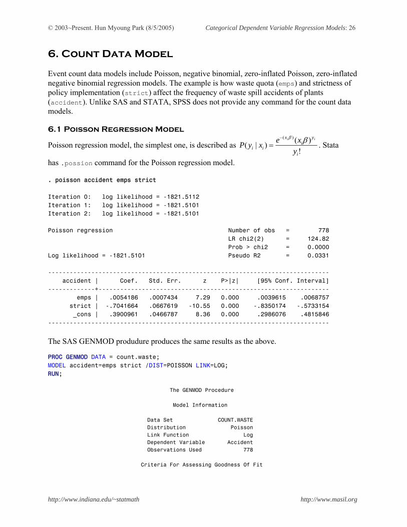
6. Count Data Model Event count data models include Poisson, negative binomial, zero-inflated Poisson, zero-inflated negative binomial regression models. The example is how waste quota (emps) and strictness of policy implementation (strict) affect the frequency of waste spill accidents of plants (accident). Unlike SAS and STATA, SPSS does not provide any command for the count data models. 6.1 Poisson Regression Model
Poisson regression model, the simplest one, is described as !
)()|()(
i
yi
x
ii yxexyP
ii ββ−
= . Stata
has .possion command for the Poisson regression model. . poisson accident emps strict Iteration 0: log likelihood = -1821.5112 Iteration 1: log likelihood = -1821.5101 Iteration 2: log likelihood = -1821.5101 Poisson regression Number of obs = 778 LR chi2(2) = 124.82 Prob > chi2 = 0.0000 Log likelihood = -1821.5101 Pseudo R2 = 0.0331 ------------------------------------------------------------------------------ accident | Coef. Std. Err. z P>|z| [95% Conf. Interval] -------------+---------------------------------------------------------------- emps | .0054186 .0007434 7.29 0.000 .0039615 .0068757 strict | -.7041664 .0667619 -10.55 0.000 -.8350174 -.5733154 _cons | .3900961 .0466787 8.36 0.000 .2986076 .4815846 ------------------------------------------------------------------------------ The SAS GENMOD produdure produces the same results as the above. PROC GENMOD DATA = count.waste; MODEL accident=emps strict /DIST=POISSON LINK=LOG; RUN; The GENMOD Procedure Model Information Data Set COUNT.WASTE Distribution Poisson Link Function Log Dependent Variable Accident Observations Used 778 Criteria For Assessing Goodness Of Fit
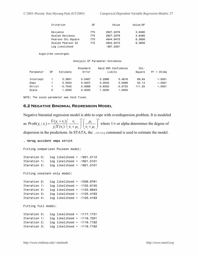
© 2003~Present. Hun Myoung Park (8/5/2005) Categorical Dependent Variable Regression Models: 27
http://www.indiana.edu/~statmath http://www.masil.org
Criterion DF Value Value/DF Deviance 775 2827.2079 3.6480 Scaled Deviance 775 2827.2079 3.6480 Pearson Chi-Square 775 4944.9473 6.3806 Scaled Pearson X2 775 4944.9473 6.3806 Log Likelihood -667.2291 Algorithm converged. Analysis Of Parameter Estimates Standard Wald 95% Confidence Chi- Parameter DF Estimate Error Limits Square Pr > ChiSq Intercept 1 0.3901 0.0467 0.2986 0.4816 69.84 <.0001 Emps 1 0.0054 0.0007 0.0040 0.0069 53.13 <.0001 Strict 1 -0.7042 0.0668 -0.8350 -0.5733 111.25 <.0001 Scale 0 1.0000 0.0000 1.0000 1.0000 NOTE: The scale parameter was held fixed. 6.2 Negative Binomial Regression Model Negative binomial regression model is able to cope with overdispersion problem. It is modeled
as ii y
ii
i
v
ii
i
ii
iiii vv
vvyvyxyob ⎟⎟
⎠
⎞⎜⎜⎝
⎛+⎟⎟
⎠
⎞⎜⎜⎝
⎛+Γ
+Γ=
µµ
µ)(!)()|(Pr where 1/v or alpha determines the degree of
dispersion in the predictions. In STATA, the .nbreg command is used to estimate the model. . nbreg accident emps strict Fitting comparison Poisson model: Iteration 0: log likelihood = -1821.5112 Iteration 1: log likelihood = -1821.5101 Iteration 2: log likelihood = -1821.5101 Fitting constant-only model: Iteration 0: log likelihood = -1256.6761 Iteration 1: log likelihood = -1152.6155 Iteration 2: log likelihood = -1125.6643 Iteration 3: log likelihood = -1125.4183 Iteration 4: log likelihood = -1125.4183 Fitting full model: Iteration 0: log likelihood = -1117.1731 Iteration 1: log likelihood = -1116.7201 Iteration 2: log likelihood = -1116.7182 Iteration 3: log likelihood = -1116.7182

© 2003~Present. Hun Myoung Park (8/5/2005) Categorical Dependent Variable Regression Models: 28
http://www.indiana.edu/~statmath http://www.masil.org
Negative binomial regression Number of obs = 778 LR chi2(2) = 17.40 Prob > chi2 = 0.0002 Log likelihood = -1116.7182 Pseudo R2 = 0.0077 ------------------------------------------------------------------------------ accident | Coef. Std. Err. z P>|z| [95% Conf. Interval] -------------+---------------------------------------------------------------- emps | .0051981 .0022595 2.30 0.021 .0007694 .0096267 strict | -.6702548 .1671191 -4.01 0.000 -.9978021 -.3427074 _cons | .3851111 .1278468 3.01 0.003 .134536 .6356861 -------------+---------------------------------------------------------------- /lnalpha | 1.37509 .0885176 1.201599 1.548582 -------------+---------------------------------------------------------------- alpha | 3.955434 .3501257 3.32543 4.704793 ------------------------------------------------------------------------------ Likelihood ratio test of alpha=0: chibar2(01) = 1409.58 Prob>=chibar2 = 0.000 Note that the last line shows the test of overdispersion with the null hypothesis of alpha=0. There is statistically significant evidence of overdispersion (p<.000), which indicates the negative binomial regression model is better than the Poisson regression model. The SAS GENMOD procedure produces the equivalent results to the above. Note that STATA calls the dispersion parameter as Alpha. PROC GENMOD DATA = count.waste; MODEL accident=emps strict /DIST=NEGBIN LINK=LOG; RUN; The GENMOD Procedure Model Information Data Set COUNT.WASTE Distribution Negative Binomial Link Function Log Dependent Variable Accident Observations Used 778 Criteria For Assessing Goodness Of Fit Criterion DF Value Value/DF Deviance 775 589.7752 0.7610 Scaled Deviance 775 589.7752 0.7610 Pearson Chi-Square 775 845.6033 1.0911 Scaled Pearson X2 775 845.6033 1.0911 Log Likelihood 37.5628 Algorithm converged.

© 2003~Present. Hun Myoung Park (8/5/2005) Categorical Dependent Variable Regression Models: 29
http://www.indiana.edu/~statmath http://www.masil.org
Analysis Of Parameter Estimates Standard Wald 95% Confidence Chi- Parameter DF Estimate Error Limits Square Pr > ChiSq Intercept 1 0.3851 0.1278 0.1345 0.6357 9.07 0.0026 Emps 1 0.0052 0.0023 0.0008 0.0096 5.29 0.0214 Strict 1 -0.6703 0.1671 -0.9978 -0.3427 16.09 <.0001 Dispersion 1 3.9554 0.3501 3.3254 4.7048 NOTE: The negative binomial dispersion parameter was estimated by maximum likelihood. The Likelihood Ratio test examines whether there is overdispersion. The ratio follows the Chi-squared distribution with one degree of freedom: )1(~)ln(ln*2 2χPoissonNB LLLR −= . The 1409.58 in the above STATA output is computed as 2*[37.5628- (-667.2291)]. Keep in mind that the null hypothesis is no overdispersion; Dispersion parameters in SAS or Alpha in STATA is zero. 6.3 Zero-Inflated Count Models In order to figure out overdispersion, zero-inflated count models assume that there are two latent groups. One is the always-zero and the other is not-always-zero. Accordingly, zero counts come from the former group and some of the latter group with a certain probability. STATA has the .zip command to estimate zero-inflated Poisson model and the .zinb command for the zero-inflated negative binomial model. Note that “inflate()” option specifies a list of variables that determine whether the observed count is zero. In SAS, there is no built-in procedure or option equivalent to the .zip. and .zinb. . zip accident emps strict, inflate(emps strict) Fitting constant-only model: Iteration 0: log likelihood = -1627.0779 Iteration 1: log likelihood = -1309.5825 Iteration 2: log likelihood = -1272.433 Iteration 3: log likelihood = -1270.9543 Iteration 4: log likelihood = -1270.9523 Iteration 5: log likelihood = -1270.9523 Fitting full model: Iteration 0: log likelihood = -1270.9523 Iteration 1: log likelihood = -1269.7219 Iteration 2: log likelihood = -1269.7206 Iteration 3: log likelihood = -1269.7206 Zero-inflated poisson regression Number of obs = 778 Nonzero obs = 280 Zero obs = 498

© 2003~Present. Hun Myoung Park (8/5/2005) Categorical Dependent Variable Regression Models: 30
http://www.indiana.edu/~statmath http://www.masil.org
Inflation model = logit LR chi2(2) = 2.46 Log likelihood = -1269.721 Prob > chi2 = 0.2918 ------------------------------------------------------------------------------ accident | Coef. Std. Err. z P>|z| [95% Conf. Interval] -------------+---------------------------------------------------------------- accident | emps | -.000277 .0008633 -0.32 0.748 -.001969 .001415 strict | -.0923911 .0729023 -1.27 0.205 -.2352771 .0504948 _cons | 1.361978 .0493222 27.61 0.000 1.265308 1.458647 -------------+---------------------------------------------------------------- inflate | emps | -.0109897 .0022678 -4.85 0.000 -.0154344 -.006545 strict | 1.057031 .1767509 5.98 0.000 .7106059 1.403457 _cons | .488656 .1211099 4.03 0.000 .2512849 .726027 ------------------------------------------------------------------------------ . zinb accident emps strict, inflate(emps strict) Fitting constant-only model: Iteration 0: log likelihood = -1190.5117 (not concave) Iteration 1: log likelihood = -1106.9874 Iteration 2: log likelihood = -1098.8642 Iteration 3: log likelihood = -1095.3638 Iteration 4: log likelihood = -1094.0237 Iteration 5: log likelihood = -1093.063 Iteration 6: log likelihood = -1092.6216 Iteration 7: log likelihood = -1091.798 Iteration 8: log likelihood = -1091.7332 Iteration 9: log likelihood = -1091.7329 Iteration 10: log likelihood = -1091.7329 Fitting full model: Iteration 0: log likelihood = -1091.7329 Iteration 1: log likelihood = -1089.5565 Iteration 2: log likelihood = -1089.5198 Iteration 3: log likelihood = -1089.5198 Zero-inflated negative binomial regression Number of obs = 778 Nonzero obs = 280 Zero obs = 498 Inflation model = logit LR chi2(2) = 4.43 Log likelihood = -1089.52 Prob > chi2 = 0.1094 ------------------------------------------------------------------------------ accident | Coef. Std. Err. z P>|z| [95% Conf. Interval] -------------+----------------------------------------------------------------

© 2003~Present. Hun Myoung Park (8/5/2005) Categorical Dependent Variable Regression Models: 31
http://www.indiana.edu/~statmath http://www.masil.org
accident | emps | -.0004407 .0020554 -0.21 0.830 -.0044691 .0035877 strict | -.3251317 .1659173 -1.96 0.050 -.6503235 .0000602 _cons | .7763065 .1508037 5.15 0.000 .4807367 1.071876 -------------+---------------------------------------------------------------- inflate | emps | -.2087768 .0955122 -2.19 0.029 -.3959772 -.0215763 strict | 7.562388 3.055775 2.47 0.013 1.573179 13.5516 _cons | .1032115 .3800045 0.27 0.786 -.6415835 .8480065 -------------+---------------------------------------------------------------- /lnalpha | .9252514 .1351387 6.85 0.000 .6603845 1.190118 -------------+---------------------------------------------------------------- alpha | 2.522502 .3408876 1.935536 3.28747 ------------------------------------------------------------------------------ 6.4 Comparison of Three Count Data Models The following plot compares the Poisson regression model, negative binomial regression model, and zero-inflated Poisson model. Note that the negative binomial and zero-inflated negative binomial models return almost the same result.
0.2
.4.6
Pre
dict
ed P
roba
bilit
y
0 2 4 6 8 10Spills Count
Observed PoissonNegative Binomial Zero Inflated Poisson
Comparison of Count Data Models
© 2003~Present. Hun Myoung Park (8/5/2005) Categorical Dependent Variable Regression Models: 32
http://www.indiana.edu/~statmath http://www.masil.org
References Allison, Paul D. 1991. Logistic Regression Using the SAS System: Theory and Application. Cary,
NC: SAS Institute. Cameron, A. Colin, and Pravin K. Trivedi. 1998. Regression Analysis of Count Data. New
York: Cambridge University Press. Greene, William H. 2000. Econometric Analysis (Fourth edition). Prentice Hall. Long, J. Scott, and Jeremy Freese. 2001. Regression Models for Categorical Dependent
Variables Using STATA. College Station, TX: STATA Press. Long, J. Scott. 1997. Regression Models for Categorical and Limited Dependent Variables.
Advanced Quantitative Techniques in the Social Sciences. Sage Publications. Maddala, G. S. 1983. Limited Dependent and Qualitative Variables in Econometrics. New York:
Cambridge University Press. SAS Institute. 2004. SAS/STAT 9.1 User's Guide. Cary, NC: SAS Institute. SPSS Inc. 2001. SPSS 11.0 Syntax Reference Guide. Chicago, IL: SPSS Inc. STATA Press. 2004. STATA Base Reference Manual, Release 8. College Station, TX: STATA
Press. Stokes, Maura E., Charles S. Davis, and Gary G. Koch. 2000. Categorical Data Analysis Using
the SAS System, 2nd ed. Cary, NC: SAS Institute. Acknowledgements I am very grateful to J. Scott Long in Sociology and David H. Good in the School of Public and Environmental Affairs, Indiana University, for their insightful and enthusiastic lectures.