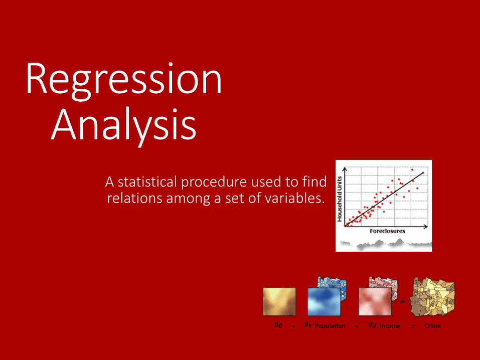
Regression Analysis

A statistical procedure used to find relations among a set of variables.

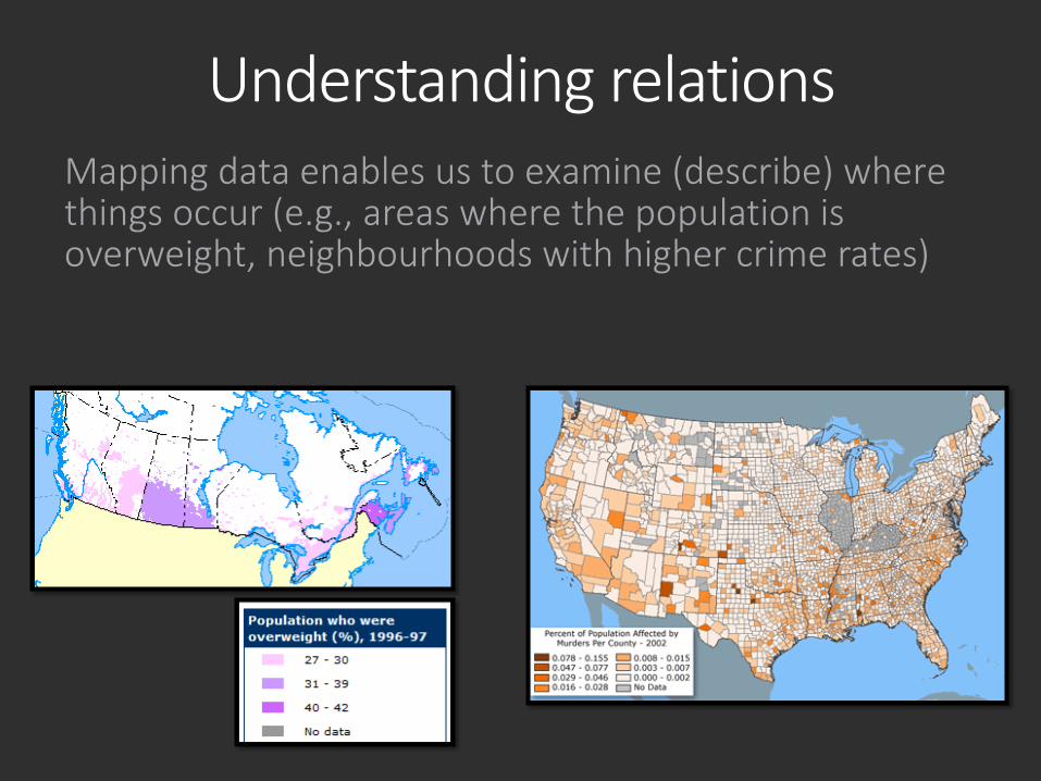
Understanding relationsMapping data enables us to examine (describe) where things occur (e.g., areas where the population is overweight, neighbourhoods with higher crime rates)

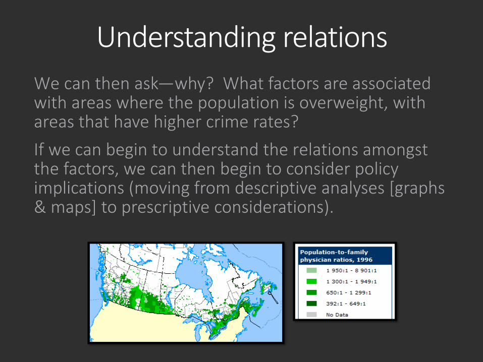
Understanding relationsWe can then ask—why? What factors are associated with areas where the population is overweight, with areas that have higher crime rates?If we can begin to understand the relations amongst the factors, we can then begin to consider policy implications (moving from descriptive analyses [graphs & maps] to prescriptive considerations).

Understanding relations

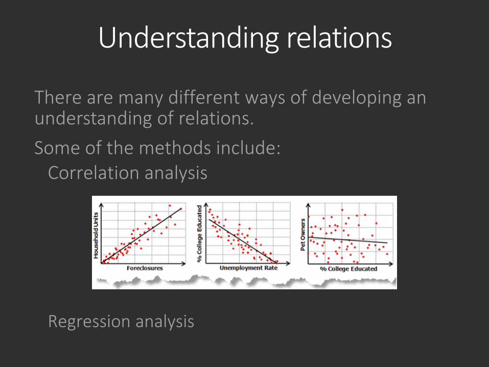
There are many different ways of developing an understanding of relations.Some of the methods include:

Correlation analysis

Regression analysis

Understanding relations

Regression analysis allows you to model, examine, and explore spatial relations and can help explain the factors behind observed spatial patterns.

You may want to understand what factors contribute to higher numbers of overweight people, to higher crime rates.

By modeling spatial relations, however, regression analysis can also be used for prediction. Modeling the factors that contribute to obesity can help planners identify how policy could help reduce obesity rates.

You might also use regression to examine the factors that relate biodiversity losses to landscape changes (Fragstats).

Regression analysisOrdinary Least Squares (OLS) is the best known of all regression techniques. It is also the traditional starting point for all spatial regression analyses. It provides a global model of the variable or process you are trying to understand or predict (obesity/biodiversity loss); it creates a single regression equation to represent that process.Geographically weighted regression (GWR) is one of several spatial regression techniques increasingly used in geography and other disciplines. GWR provides a localmodel of the variable or process you are trying to understand/predict by fitting a regression equation to every feature in the dataset.

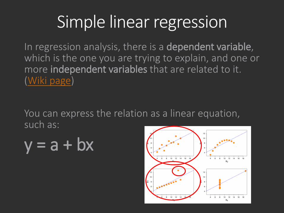
Simple linear regressionIn regression analysis, there is a dependent variable, which is the one you are trying to explain, and one or more independent variables that are related to it. (Wiki page)

You can express the relation as a linear equation, such as:

y = a + bx

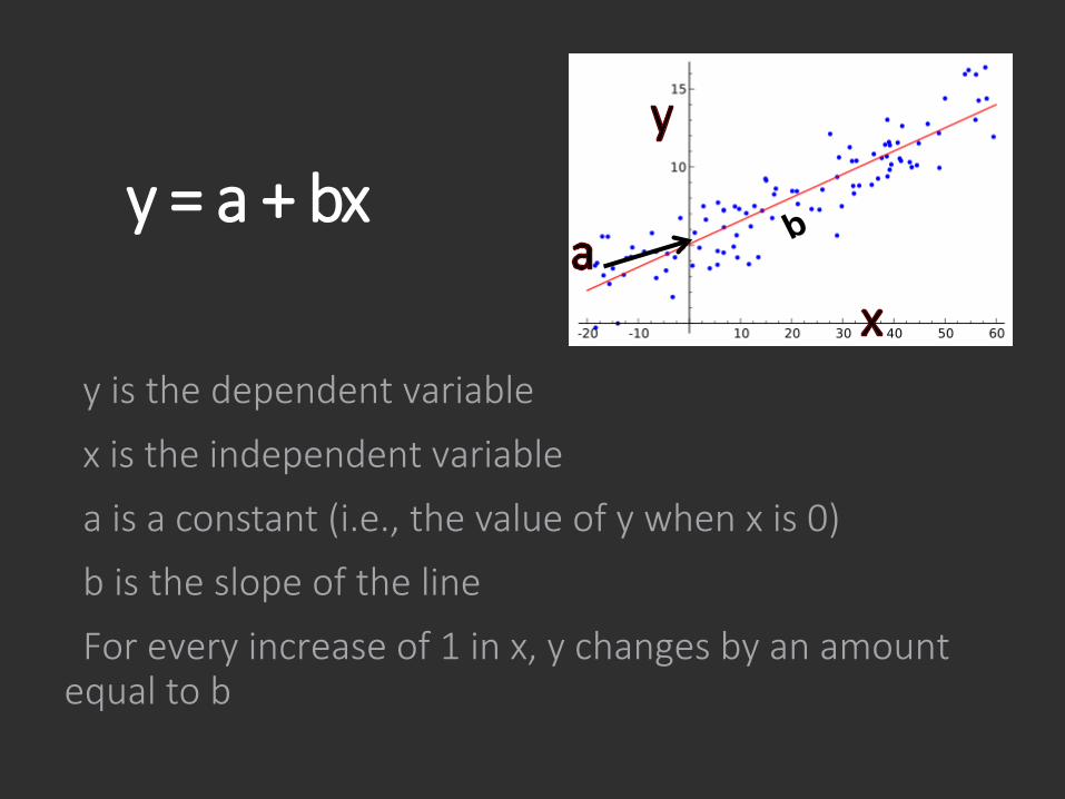
y = a + bx

y is the dependent variable

x is the independent variable

a is a constant (i.e., the value of y when x is 0)

b is the slope of the line

For every increase of 1 in x, y changes by an amount equal to b

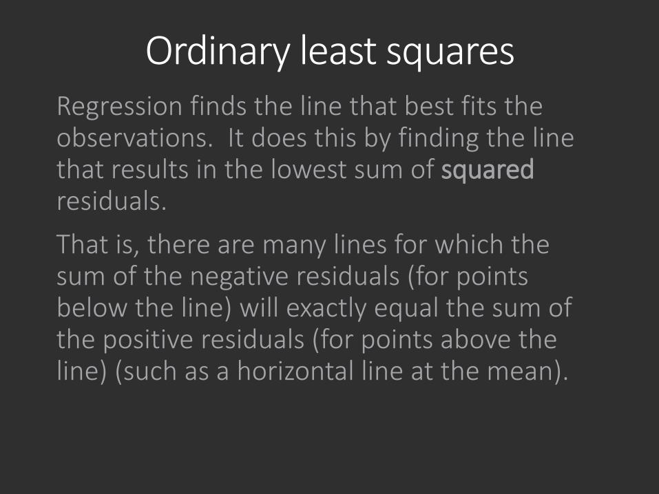
Ordinary least squaresRegression finds the line that best fits the observations. It does this by finding the line that results in the lowest sum of squaredresiduals. That is, there are many lines for which the sum of the negative residuals (for points below the line) will exactly equal the sum of the positive residuals (for points above the line) (such as a horizontal line at the mean).

Ordinary least squares

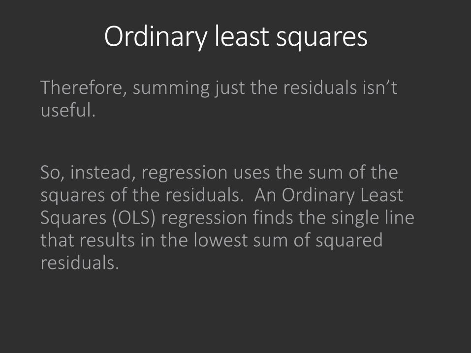
Therefore, summing just the residuals isn’t useful.

So, instead, regression uses the sum of the squares of the residuals. An Ordinary Least Squares (OLS) regression finds the single line that results in the lowest sum of squared residuals.

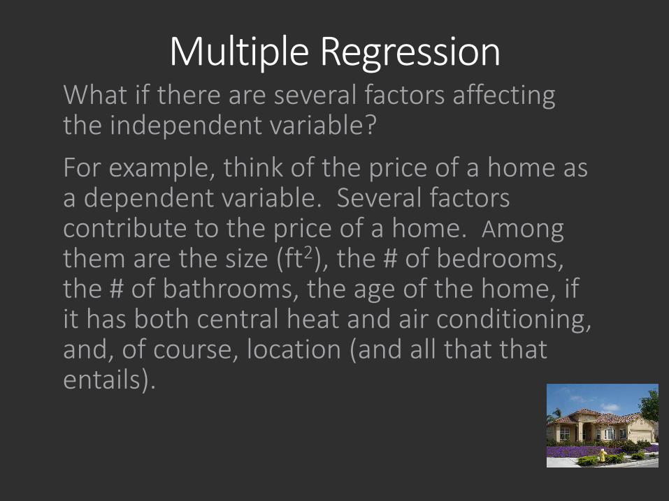
Multiple RegressionWhat if there are several factors affecting the independent variable?For example, think of the price of a home as a dependent variable. Several factors contribute to the price of a home. Among them are the size (ft2), the # of bedrooms, the # of bathrooms, the age of the home, if it has both central heat and air conditioning, and, of course, location (and all that that entails).

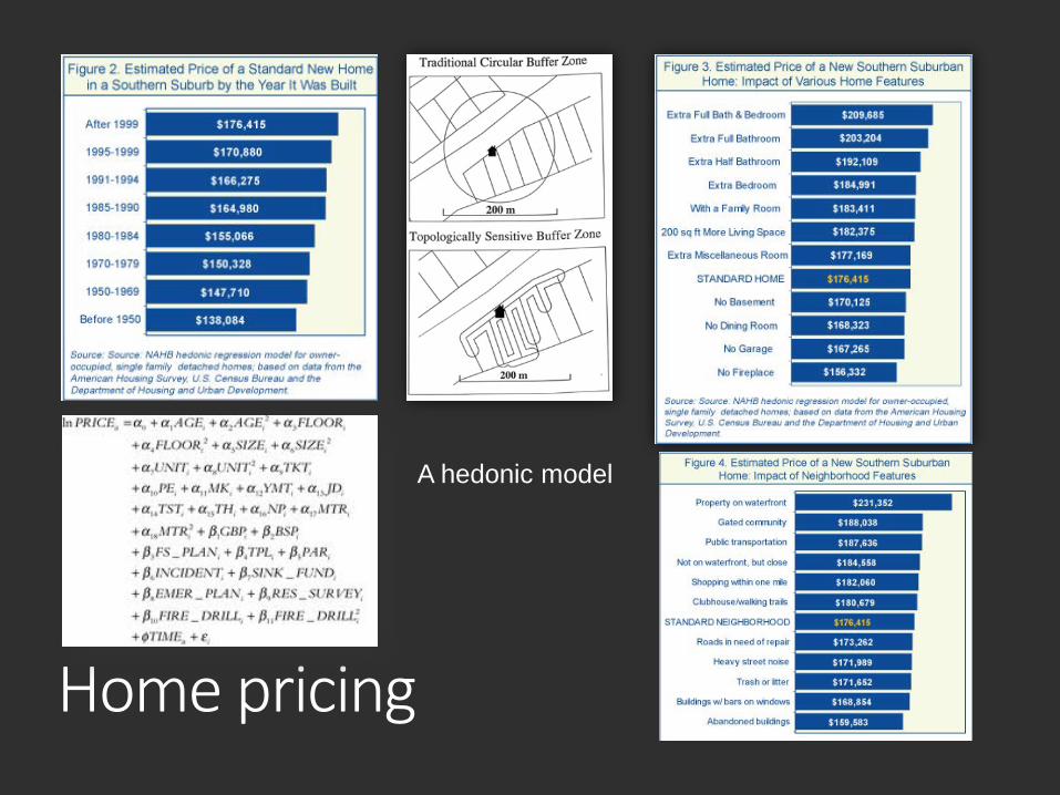
Home pricing

A hedonic model

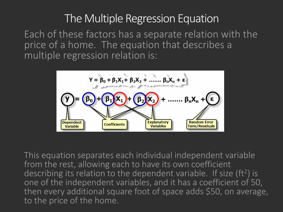
The Multiple Regression EquationEach of these factors has a separate relation with the price of a home. The equation that describes a multiple regression relation is:

This equation separates each individual independent variable from the rest, allowing each to have its own coefficient describing its relation to the dependent variable. If size (ft2) is one of the independent variables, and it has a coefficient of 50, then every additional square foot of space adds $50, on average, to the price of the home.

How Do You Run a Regression?

In a multiple regression analysis of home prices, you take data from actual homes that have sold recently. You include the selling price, as well as the values for the independent variables (square footage, # of bedrooms, etc.).

The multiple regression analysis finds the coefficients for each independent variable so that they make the line that has the lowest sum of squared residuals (in n-dimensional space, where n = # of independent variables).

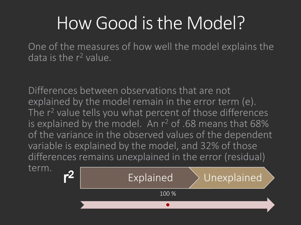
How Good is the Model?One of the measures of how well the model explains the data is the r2 value.

Differences between observations that are not explained by the model remain in the error term (e). The r2 value tells you what percent of those differences is explained by the model. An r2 of .68 means that 68% of the variance in the observed values of the dependent variable is explained by the model, and 32% of those differences remains unexplained in the error (residual) term.

Explained Unexplained100 %

Sometimes there’s no accounting for taste

Some of the error is random, and no model will explain it. A prospective homebuyer might value a basement playroom more than other people because it reminds her of her grandmother’s house where she played as a child. This can’t be observed or measured, and these types of effects will vary randomly and unpredictably. Some variance will always remain in the error term. As long as it is random, it is of no concern.

Some of the error isn’t errorSome of the error is best described as unexplained residual—if we added additional variables (such as, for homes in Vancouver, the high school catchment that the home lies within) we might be able to reduce the residual. (See the discussion below on omitted variables.)

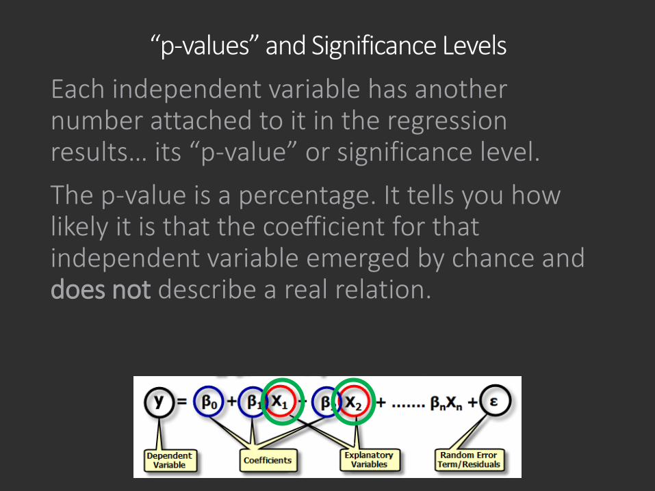
“p-values” and Significance LevelsEach independent variable has another number attached to it in the regression results… its “p-value” or significance level.The p-value is a percentage. It tells you how likely it is that the coefficient for that independent variable emerged by chance and does not describe a real relation.

“p-values” and Significance Levels

A p-value of .05 means that there is a 5% chance that the relation emerged randomly and a 95% chance that the relationship is real.

It is generally accepted practice to consider variables with a p-value of less than .05 as significant, though the only basis for this cutoff is convention.

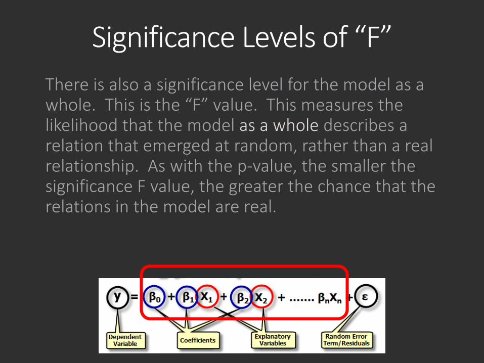
Significance Levels of “F”There is also a significance level for the model as a whole. This is the “F” value. This measures the likelihood that the model as a whole describes a relation that emerged at random, rather than a real relationship. As with the p-value, the smaller the significance F value, the greater the chance that the relations in the model are real.

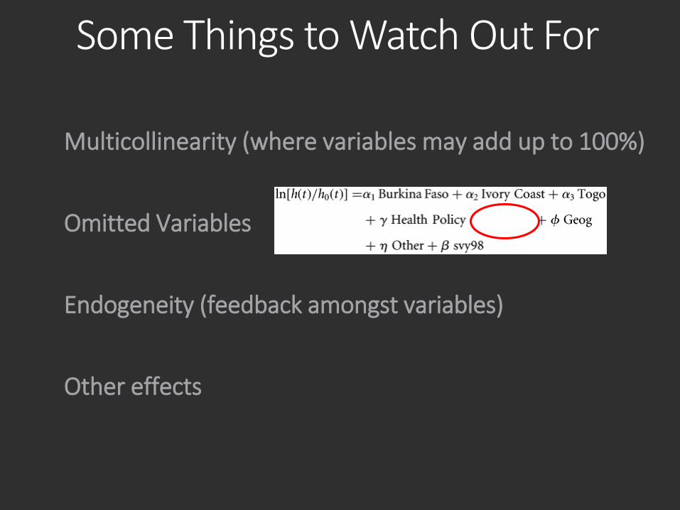
Some Things to Watch Out For

Multicollinearity (where variables may add up to 100%)

Omitted Variables

Endogeneity (feedback amongst variables)

Other effects

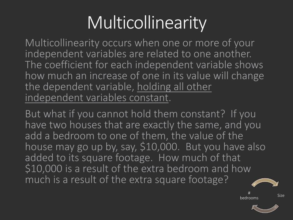
MulticollinearityMulticollinearity occurs when one or more of your independent variables are related to one another. The coefficient for each independent variable shows how much an increase of one in its value will change the dependent variable, holding all other independent variables constant. But what if you cannot hold them constant? If you have two houses that are exactly the same, and you add a bedroom to one of them, the value of the house may go up by, say, $10,000. But you have also added to its square footage. How much of that $10,000 is a result of the extra bedroom and how much is a result of the extra square footage?

Size# bedrooms

Multicollinearity

If the variables are very closely related, and/or if you have only a small number of observations, it can be difficult to separate these effects. Your regression derives the coefficients that best describe your set of data, but the independent variables may not have a valid p-value if multicollinearity is present.

This is often assessed using correlation values.

The Variance Inflation Factor (VIF) is used to judge how significant the multicollinearity is.

MulticollinearitySometimes it may be appropriate to remove a variable that is related to others, but it may not always be appropriate. In our home value example, both the number of bedrooms and the square footage are important on their own, in addition to whatever combined effects they may have. Removing one variable may be worse than leaving it in. This does not necessarily mean that the model as a whole is problematic, but it may mean that the model should not be used to draw conclusions about the relation of individual independent variables with the dependent variable.

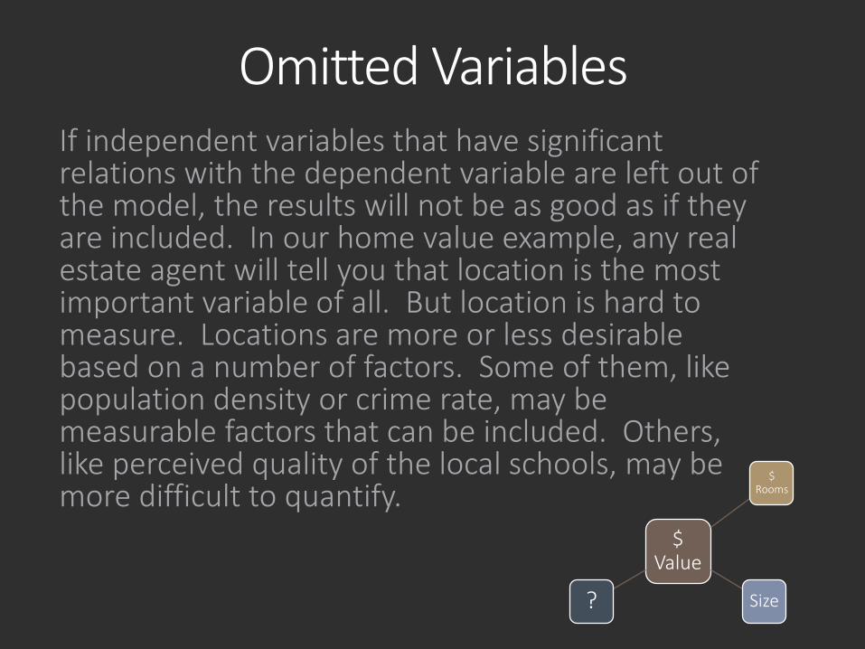
Omitted VariablesIf independent variables that have significant relations with the dependent variable are left out of the model, the results will not be as good as if they are included. In our home value example, any real estate agent will tell you that location is the most important variable of all. But location is hard to measure. Locations are more or less desirable based on a number of factors. Some of them, like population density or crime rate, may be measurable factors that can be included. Others, like perceived quality of the local schools, may be more difficult to quantify.

$ Value

$ Rooms

Size?

Omitted VariablesYou must also decide what level of specificity to use. Do you use the crime rate for the neighbourhood, the postal code, the street? Is the data even available at the level of specificity you want to use? These factors can lead to omitted variable bias—variance in the error term (e) that is not random and that could be explained by an independent variable that is not in the model (geography often is an omitted variable).

Such bias can distort the coefficients on the other independent variables, as well as decreasing the r2 and increasing the F. Sometimes data just isn’t available, and some variables aren’t measurable. There are methods for reducing the bias from omitted variables, but it can’t always be completely corrected.

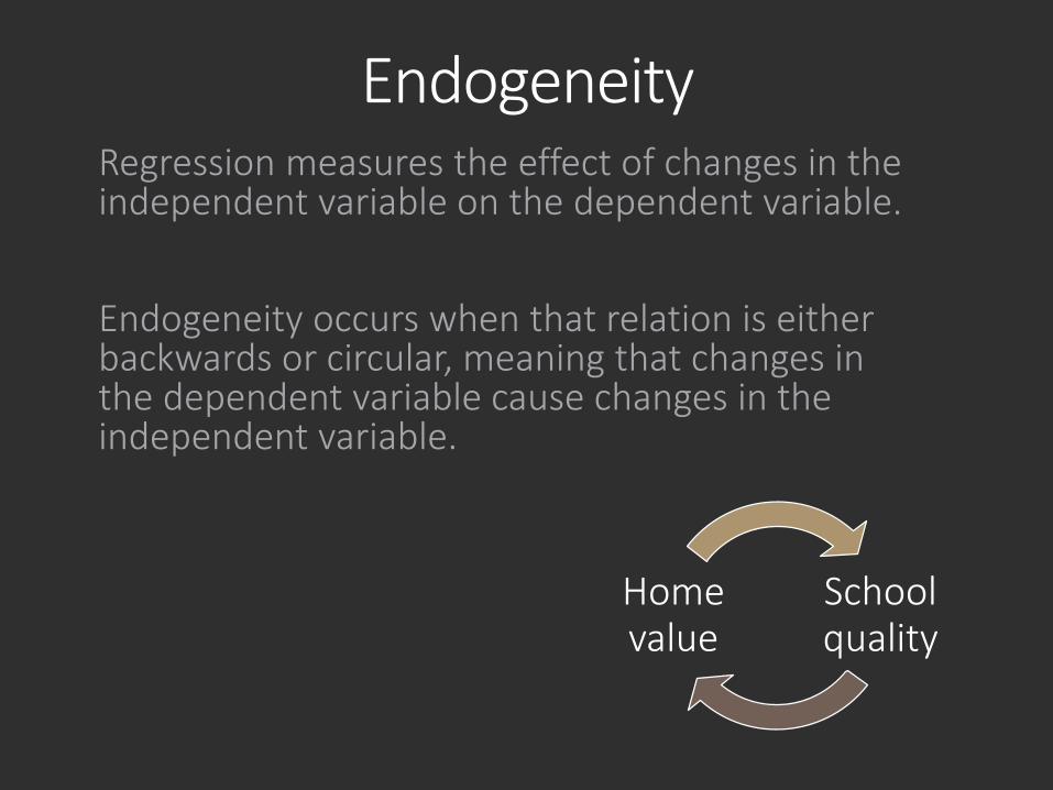
EndogeneityRegression measures the effect of changes in the independent variable on the dependent variable.

Endogeneity occurs when that relation is either backwards or circular, meaning that changes in the dependent variable cause changes in the independent variable.

School quality

Home value

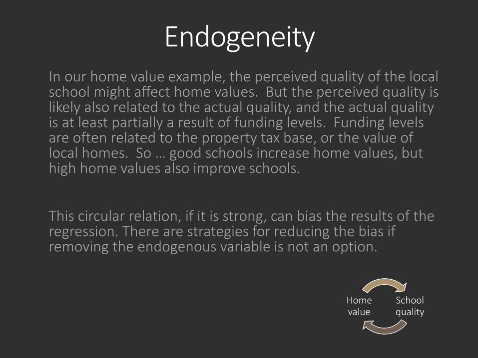
EndogeneityIn our home value example, the perceived quality of the local school might affect home values. But the perceived quality is likely also related to the actual quality, and the actual quality is at least partially a result of funding levels. Funding levels are often related to the property tax base, or the value of local homes. So … good schools increase home values, but high home values also improve schools.

This circular relation, if it is strong, can bias the results of the regression. There are strategies for reducing the bias if removing the endogenous variable is not an option.

School quality

Home value

Other effects

There are several other types of biases or sources of distortion that can exist in a model for a variety of reasons. Spatial autocorrelation is one significant bias that can greatly affect aspatial regression. There are tests to measure the levels of bias, and there are strategies that can be used to reduce it. Eventually, though, one may have to accept a certain amount of bias in the final model, especially when there are data limitations. In that case, the best that can be done is to describe the problem and the effects it might have when presenting the model.

Geographically-weighted regression

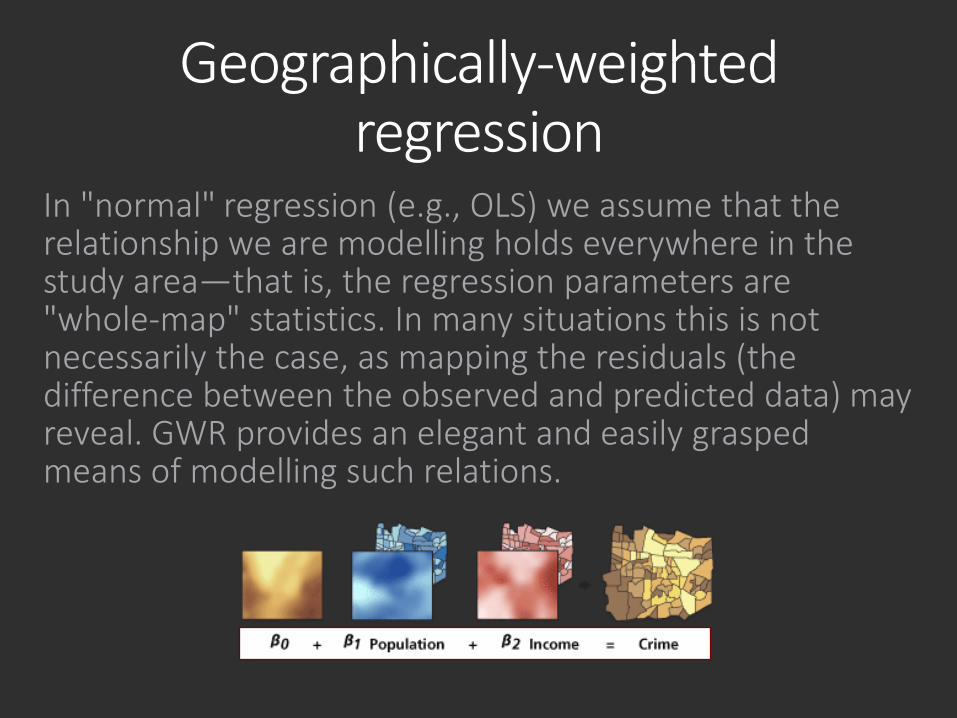
In "normal" regression (e.g., OLS) we assume that the relationship we are modelling holds everywhere in the study area—that is, the regression parameters are "whole-map" statistics. In many situations this is not necessarily the case, as mapping the residuals (the difference between the observed and predicted data) may reveal. GWR provides an elegant and easily grasped means of modelling such relations.

Geographically-weighted regression

Geographically Weighted Regression (GWR) is one of several spatial regression techniques increasingly used in geography and other disciplines. GWR provides a local model of the variable or process you are trying to understand/predict by fitting a regression equation to every feature in the dataset. GWR constructs these separate equations by incorporating the dependent and explanatory variables of features falling within the bandwidth of each target feature. The shape and size of the bandwidth is dependent on user input for the Kernel type, Bandwidth method, Distance, and Number of neighbors parameters.

Geographically-weighted regression

GWR permits the parameter estimates to vary locally; we can rewrite the (now nonspatialregression) model in a slightly different form:

y(g) = b0(g) + b1(g)x1 + b2(g)x2 + e

where (g) indicates that the parameters are to be estimated at a location whose coordinates are given by the vector g (e.g., [UTMeasting, UTMnorthing]).

In standard applications of regression, a dependent variable is linked to a set of independent variables with one of the main outputs of regression being the estimation of a parameter that links each independent variable to the dependent variable. A major problem with this technique when applied to spatial data is that the processes being examined are assumed to be constant over space – that is, one model fits all.

GWR allows for the modelling of processes that vary over space. GWR results in a set of local parameter estimates for each relationship which can be mapped to produce a parameter surface across the study region. In this way, GWR provides valuable information on the nature of the processes being investigated and supersedes traditional global types of regression modelling.

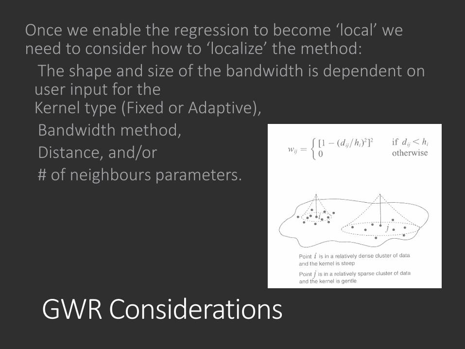
GWR Considerations

Once we enable the regression to become ‘local’ we need to consider how to ‘localize’ the method:

The shape and size of the bandwidth is dependent on user input for the Kernel type (Fixed or Adaptive), Bandwidth method, Distance, and/or # of neighbours parameters.

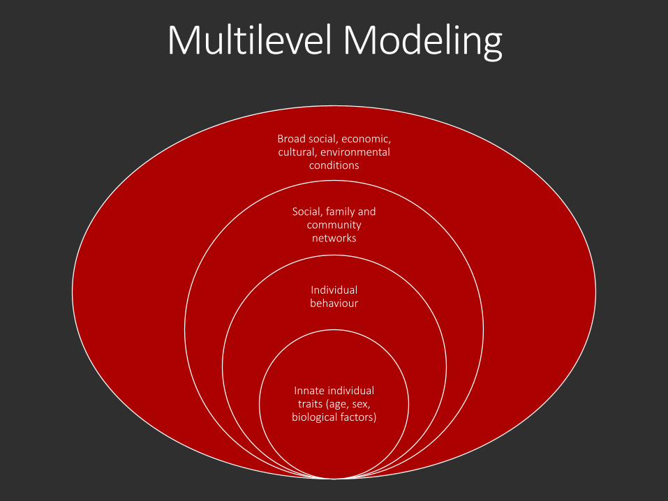
Multilevel Modeling

Broad social, economic, cultural, environmental

conditions

Social, family and community networks

Individual behaviour

Innate individual traits (age, sex,

biological factors)

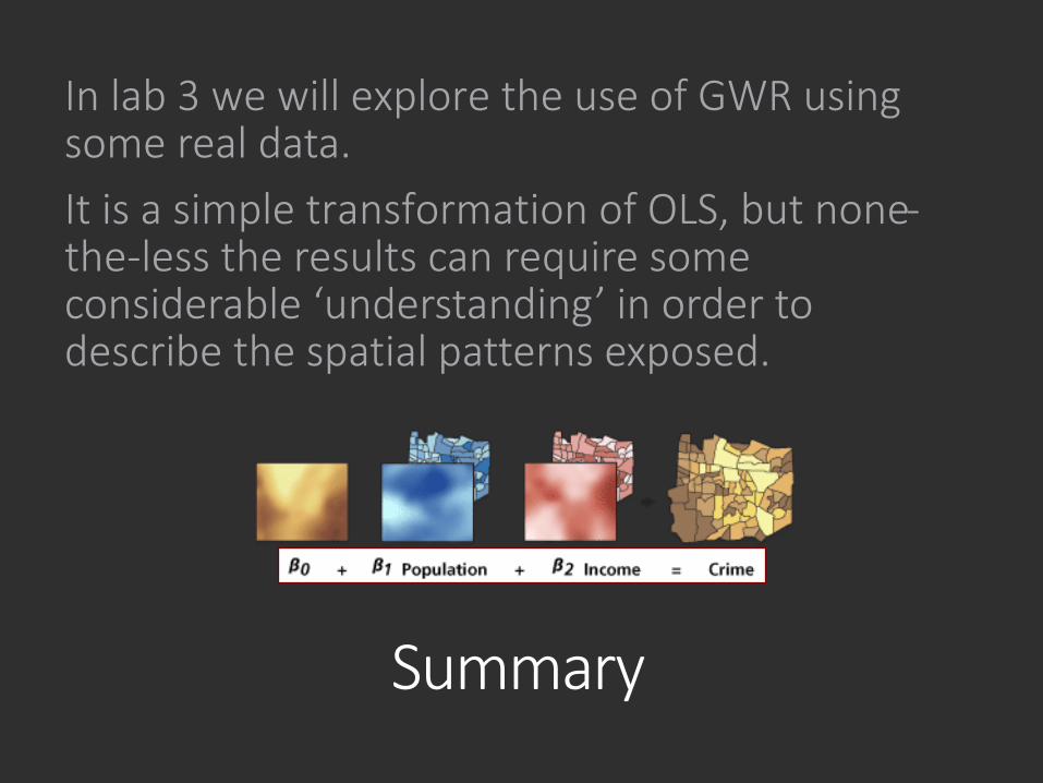
Summary

In lab 3 we will explore the use of GWR using some real data.It is a simple transformation of OLS, but none-the-less the results can require some considerable ‘understanding’ in order to describe the spatial patterns exposed.