morfismos, vol 17, no 1, 2013
DESCRIPTION
Morfismos issue for June 2013TRANSCRIPT
VOLUMEN 17NÚMERO 1
ENERO A JUNIO DE 2013ISSN: 1870-6525

Chief Editors - Editores Generales
• Isidoro Gitler • Jesus Gonzalez
Associate Editors - Editores Asociados
• Ruy Fabila • Ismael Hernandez• Onesimo Hernandez-Lerma • Hector Jasso Fuentes
• Sadok Kallel • Miguel Maldonado• Carlos Pacheco • Enrique Ramırez de Arellano
• Enrique Reyes • Dai Tamaki• Enrique Torres Giese
Apoyo Tecnico
• Adriana Aranda Sanchez • Juan Carlos Castro Contreras• Irving Josue Flores Romero • Omar Hernandez Orozco
• Roxana Martınez • Laura Valencia
Morfismos esta disponible en la direccion http://www.morfismos.cinvestav.mx.Para mayores informes dirigirse al telefono +52 (55) 5747-3871. Toda corres-pondencia debe ir dirigida a la Sra. Laura Valencia, Departamento de Matema-ticas del Cinvestav, Apartado Postal 14-740, Mexico, D.F. 07000, o por correoelectronico a la direccion: [email protected].
VOLUMEN 17NÚMERO 1
ENERO A JUNIO DE 2013ISSN: 1870-6525

Morfismos, Volumen 17, Numero 1, enero a junio 2013, es una publicacionsemestral editada por el Centro de Investigacion y de Estudios Avanzadosdel Instituto Politecnico Nacional (Cinvestav), a traves del Departamentode Matematicas. Av. Instituto Politecnico Nacional No. 2508, Col. San PedroZacatenco, Delegacion Gustavo A. Madero, C.P. 07360, D.F., Tel. 55-57473800,www.cinvestav.mx, [email protected], Editores Generales: Drs.Isidoro Gitler y Jesus Gonzalez Espino Barros. Reserva de DerechosNo. 04-2012-011011542900-102, ISSN: 1870-6525, ambos otorgados por elInstituto Nacional del Derecho de Autor. Certificado de Licitud de TıtuloNo. 14729, Certificado de Licitud de Contenido No. 12302, ambos otorga-dos por la Comision Calificadora de Publicaciones y Revistas Ilustradas de laSecretarıa de Gobernacion. Impreso por el Departamento de Matematicas delCinvestav, Avenida Instituto Politecnico Nacional 2508, Colonia San PedroZacatenco, C.P. 07360, Mexico, D.F. Este numero se termino de imprimir enjulio de 2013 con un tiraje de 50 ejemplares.
Las opiniones expresadas por los autores no necesariamente reflejan lapostura de los editores de la publicacion.
Queda estrictamente prohibida la reproduccion total o parcial de los con-tenidos e imagenes de la publicacion, sin previa autorizacion del Cinvestav.


Information for Authors
The Editorial Board of Morfismos calls for papers on mathematics and related areas tobe submitted for publication in this journal under the following guidelines:
• Manuscripts should fit in one of the following three categories: (a) papers covering thegraduate work of a student, (b) contributed papers, and (c) invited papers by leadingscientists. Each paper published in Morfismos will be posted with an indication ofwhich of these three categories the paper belongs to.
• Papers in category (a) might be written in Spanish; all other papers proposed forpublication in Morfismos shall be written in English, except those for which theEditoral Board decides to publish in another language.
• All received manuscripts will be refereed by specialists.
• In the case of papers covering the graduate work of a student, the author shouldprovide the supervisor’s name and affiliation, date of completion of the degree, andinstitution granting it.
• Authors may retrieve the LATEX macros used for Morfismos through the web sitehttp://www.math.cinvestav.mx, at “Revista Morfismos”. The use by authors of thesemacros helps for an expeditious production process of accepted papers.
• All illustrations must be of professional quality.
• Authors will receive the pdf file of their published paper.
• Manuscripts submitted for publication in Morfismos should be sent to the email ad-dress [email protected].
Informacion para Autores
El Consejo Editorial de Morfismos convoca a proponer artıculos en matematicas y areasrelacionadas para ser publicados en esta revista bajo los siguientes lineamientos:
• Se consideraran tres tipos de trabajos: (a) artıculos derivados de tesis de grado dealta calidad, (b) artıculos por contribucion y (c) artıculos por invitacion escritos porlıderes en sus respectivas areas. En todo artıculo publicado en Morfismos se indicarael tipo de trabajo del que se trate de acuerdo a esta clasificacion.
• Los artıculos del tipo (a) podran estar escritos en espanol. Los demas trabajos deberanestar redactados en ingles, salvo aquellos que el Comite Editorial decida publicar enotro idioma.
• Cada artıculo propuesto para publicacion en Morfismos sera enviado a especialistaspara su arbitraje.
• En el caso de artıculos derivados de tesis de grado se debe indicar el nombre delsupervisor de tesis, su adscripcion, la fecha de obtencion del grado y la institucionque lo otorga.
• Los autores interesados pueden obtener el formato LATEX utilizado por Morfismos enel enlace “Revista Morfismos” de la direccion http://www.math.cinvestav.mx. La uti-lizacion de dicho formato ayudara en la pronta publicacion de los artıculos aceptados.
• Si el artıculo contiene ilustraciones o figuras, estas deberan ser presentadas de formaque se ajusten a la calidad de reproduccion de Morfismos.
• Los autores recibiran el archivo pdf de su artıculo publicado.
• Los artıculos propuestos para publicacion en Morfismos deben ser dirigidos a la di-reccion [email protected].
Editorial Guidelines
Morfismos is the journal of the Mathematics Department of Cinvestav. Oneof its main objectives is to give advanced students a forum to publish their earlymathematical writings and to build skills in communicating mathematics.
Publication of papers is not restricted to students of Cinvestav; we want to en-courage students in Mexico and abroad to submit papers. Mathematics researchreports or summaries of bachelor, master and Ph.D. theses of high quality will beconsidered for publication, as well as contributed and invited papers by researchers.All submitted papers should be original, either in the results or in the methods.The Editors will assign as referees well-established mathematicians, and the accep-tance/rejection decision will be taken by the Editorial Board on the basis of thereferee reports.
Authors of Morfismos will be able to choose to transfer copy rights of theirworks to Morfismos. In that case, the corresponding papers cannot be consideredor sent for publication in any other printed or electronic media. Only those papersfor which Morfismos is granted copyright will be subject to revision in internationaldata bases such as the American Mathematical Society’s Mathematical Reviews, andthe European Mathematical Society’s Zentralblatt MATH.
Morfismos
Lineamientos Editoriales
Morfismos, revista semestral del Departamento de Matematicas del Cinvestav,tiene entre sus principales objetivos el ofrecer a los estudiantes mas adelantadosun foro para publicar sus primeros trabajos matematicos, a fin de que desarrollenhabilidades adecuadas para la comunicacion y escritura de resultados matematicos.
La publicacion de trabajos no esta restringida a estudiantes del Cinvestav; de-seamos fomentar la participacion de estudiantes en Mexico y en el extranjero, asıcomo de investigadores mediante artıculos por contribucion y por invitacion. Losreportes de investigacion matematica o resumenes de tesis de licenciatura, maestrıao doctorado de alta calidad pueden ser publicados en Morfismos. Los artıculos apublicarse seran originales, ya sea en los resultados o en los metodos. Para juzgaresto, el Consejo Editorial designara revisores de reconocido prestigio en el orbe in-ternacional. La aceptacion de los artıculos propuestos sera decidida por el ConsejoEditorial con base a los reportes recibidos.
Los autores que ası lo deseen podran optar por ceder a Morfismos los derechos depublicacion y distribucion de sus trabajos. En tal caso, dichos artıculos no podranser publicados en ninguna otra revista ni medio impreso o electronico. Morfismossolicitara que tales artıculos sean revisados en bases de datos internacionales como loson el Mathematical Reviews, de la American Mathematical Society, y el ZentralblattMATH, de la European Mathematical Society.
Morfismos

Contents - Contenido
Partial monoids and Dold-Thom functors
Jacob Mostovoy . . . . . . . . . . . . . . . . . . . . . . . . . . . . . . . . . . . . . . . . . . . . . . . . . . . . . . . . . . 1
Algebra C∗ generada por operadores de Toeplitz con sımbolos discontinuos enel espacio de Bergman armonico
Maribel Loaiza and Carmen Lozano . . . . . . . . . . . . . . . . . . . . . . . . . . . . . . . . . . . . . 19
Ideals, varieties, stability, colorings and combinatorial designs
Javier Munoz, Feliu Sagols, and Charles J. Colbourn . . . . . . . . . . . . . . . . . . . . 41

Morfismos, Vol. 17, No. 1, 2013, pp. 1–18
Partial monoids and Dold-Thom functors ∗
Jacob Mostovoy 1
Abstract
Dold-Thom functors generalize infinite symmetric products, whereinteger multiplicities of points are replaced by composable ele-ments of a partial abelian monoid. It is well-known that for anyconnective homology theory, the machinery of Γ-spaces producesthe corresponding linear Dold-Thom functor. In this note we con-struct such functors directly from spectra by exhibiting a partialmonoid corresponding to a spectrum.
2000 Mathematics Subject Classification: Primary 55N20, Secondary22A30.Keywords and phrases: Dold-Thom functors, symmetric products, gen-eralized homology.
1 Introduction
Let SP∞X be the infinite symmetric product of a pointed connectedcell complex X. Then, according to the Dold-Thom Theorem [4], thehomotopy groups of SP∞X coincide, as a functor, with the reducedsingular homology of X. Although there is no computational advantagein this definition of singular homology, it is important since it can beextended to the algebro-geometric context; in particular, the motiviccohomology of [9] is defined in this way.
The construction of the infinite symmetric product can be general-ized so as to produce an arbitrary connective homology theory. Suchgeneralized symmetric products were defined by G. Segal in [11]: essen-tially, these are labelled configuration spaces, with labels in a Γ-space
∗Invited paper.1This work was partially supported by the CONACyT grant no. 44100.
1

2 Jacob Mostovoy
(see also [2, 3, 6]). If the Γ-space of labels is injective (see [13]) it givesrise to a partial abelian monoid; it has been proved that in [13] that foreach connective homology theory there exists an injective Γ-space. Inthis case Segal’s generalized symmetric product can be thought of as aspace of configurations of points labelled by composable elements of apartial monoid. An explicit example discussed in [12] is the space of con-figurations of points labelled by orthogonal vector spaces: it producesconnective K-theory.
We shall call the generalized symmetric product functor with pointshaving labels, or “multiplicities”, in a partial monoid M , the Dold-Thom functor with coefficients in M . Certainly, the construction ofsuch functors via Γ-spaces is most appealing. However, if we start witha spectrum, constructing the corresponding Dold-Thom functor usingΓ-spaces is not an entirely straightforward procedure since the Γ-spacenaturally associated to a spectrum is not injective. The purpose ofthe present note is to show how a connective spectrum M gives riseto an explicit partial monoid M such that the homotopy of the Dold-Thom functor with coefficients in M coincides, as a functor, with thehomology with coefficients in M. The construction is based on a trivialobservation: if Y is a space and X is a pointed space, the space of mapsfrom Y to X has a commutative partial multiplication with a unit.
2 Partial monoids and infinite loop spaces
2.1 Partial monoids.
Most of the following definitions appear in [10]. A partial monoid Mis a topological space equipped with a subspace M(2) ⊆ M × M andan addition map M(2) → M , written as (m1,m2) → m1 + m2, andsatisfying the following two conditions:
• there exists 0 ∈ M such that 0 +m and m+ 0 are defined for allm ∈ M and such that 0 +m = m+ 0 = m;
• for all m1,m2 and m3 the sum m1+(m2+m3) is defined whenever(m1 +m2) +m3 is defined, and both are equal.
We shall say that a partial monoid is abelian if for all m1 and m2 suchthat m1 +m2 is defined, m2 +m1 is also defined, and both expressionsare equal.

Partial monoids and Dold-Thom functors 3
The classifying space BM of a partial monoid M is defined asfollows. Let M(k) be the subspace of Mk consisting of composablek-tuples. The M(k) form a simplicial space, with the face operators∂i : M(k) → M(k−1) and the degeneracy operators si : M(k) → M(k+1)
defined as
∂i(m1, . . . ,mk) = (m2, . . . ,mk) if i = 0= (m1, . . . ,mi +mi+1, . . . ,mk) if 0 < i < k= (m1, . . . ,mk−1) if i = k
and
si(m1, . . . ,mk) = (m1, . . . ,mi, 0,mi+1, . . . ,mk) if 0 ≤ i ≤ k.
The classifying space BM is the realization of this simplicial space. Inthe case when M is a monoid, BM is its usual classifying space. IfM is a partial monoid with a trivial multiplication (that is, the onlycomposable pairs of elements in M are those containing 0), the spaceBM coincides with the reduced suspension ΣM .
A homomorphism f : M → N is a map such that whenever m1+m2
is defined, f(m1)+f(m2) is also defined and equal to f(m1+m2). If f ,considered as a map of sets, is an inclusion, we say that M is a partialsubmonoid of N .
2.2 Partial monoids and spectra.
Given a pointed space X we shall write ΩX for the space all mapsR → X supported (that is, attaining a value distinct from the basepoint of X) inside a compact subset of R. If ΩεX denotes the space ofall maps R → X supported in [−ε, ε], with the compact-open topology,ΩX is given the weak topology of the union ∪εΩεX. The usual loopspace can be identified with Ω1X and the inclusion Ω1X → ΩX is ahomotopy equivalence.
If X is an abelian partial monoid and Y is a space, the space of allcontinuous maps Y → X is also an abelian partial monoid. Two mapsf, g are composable in this partial monoid if at each point of Y theirvalues are composable. In particular, ifX is a pointed topological space,then, considering X as a monoid with the trivial multiplication, we seethat ΩX is an abelian partial monoid; two maps in ΩX are composableif their supports are disjoint.
The space ΩX as defined here is much better behaved with respectto this partial multiplication than the usual loop space: while a generic

4 Jacob Mostovoy
element of the usual loop space is only composable with the base point,each element of ΩX is composable with a big (in a sense that we neednot make precise here) subset of ΩX.
The partial multiplication on ΩnX for n > 1 can be defined induc-tively for all the pairs of maps from R to the partial monoid Ωn−1Xwhose values are composable at each point. This is, of course, the sameas treating the points of ΩnX as maps Rn → X and defining the com-posable pairs of maps as those with disjoint supports in Rn.
Let nowM be a connective spectrum. We construct a partial abelianmultiplication on its infinite loop space as follows. First, let us replaceinductively M0 by a point and the spaces Mi for i > 0 by the mappingcylinders of the structure maps
ΣMi−1 → Mi,
obtaining a spectrum M′. This, in particular, allows us to assumethat all the structure maps are inclusions. As a consequence, we haveinclusion maps
Ωi−1M′i−1 → ΩiM′
i,
which send composable k-tuples of elements to composable k-tuples forall k. The union of all the spaces
M [i] = ΩiM′i
is the infinite loop space for the spectrum M and it naturally has thestructure of a partial abelian monoid.
2.3 Dold-Thom functors.
Let M be an abelian partial moniod and X a topological space withthe base point ∗. We define the configuration space Mn[X] of at mostn points in X with labels in M as follows. For n > 0 let Wn be thesubspace of the symmetric product SPn(X ∧ M) consisting of points∑n
i=1(xi,mi) such that the mi are composable; W0 is defined to be apoint. The space Mn[X] is the quotient of Wn by the relations
(x,m1) + (x,m2) + . . . = (x,m1 +m2) + . . . ,
where the omitted terms on both sides are understood to coincide, and
(x, 0) = (∗,m)

Partial monoids and Dold-Thom functors 5
for all x and m. This quotient map commutes with the inclusions ofWn into Wn+1 coming, in turn, from the inclusions SPn(X ∧ M) →SPn+1(X ∧M), and, hence, Mn[X] is a subspace of Mn+1[X].
The Dold-Thom functor of X with coefficients in M is the space
M [X] =⋃n>0
Mn[X].
The Dold-Thom functor with coefficients in the monoid of non-negative integers is the infinite symmetric product. If M has trivialmultiplication, we have
M [X] = M1[X] = X ∧M.
The composability of labels in a configuration is essential for thefunctoriality of M [X]. A based map f : X → Y induces a mapM [f ] : M [X] → M [Y ] as follows: a point
∑(xi,mi) is sent to the
point∑
(yj , nj) where the label nj is equal to the sum of all the mi
such that f(xi) = yj .Apart from the infinite symmetric products, Dold-Thom functors
generalize classifying spaces: for any partial monoid M its classifyingspace BM is homeomorphic to M [S1]. To construct the homeomor-phism, take the lengths of the intervals between the particles to be thebarycentric coordinates in the simplex in BM defined by the labels ofthe particles. Similarly, the classifying space of an arbitrary Γ-space canbe constructed in this way (modulo some technical details), see Section 3of [11]. The identification of BM with M [S1] also makes sense for non-abelian monoids. The construction of a classifying space for a monoidas a space of particles on S1 was first described in [8].
In the case when M is a partial abelian monoid coming from aspectrum M it is convenient to consider a different topology on Mn[X].
Namely, we defineMn[X] as the the union of the spacesM[i]n [X] with the
weak topology. Then, as above, the Dold-Thom functor with coefficientsin M associates to a space X the space M [X] = ∪Mn[X]. The technicaladvantage provided by this modification is that for any compact space
Y the map Y → M [X] factorizes through M[i]n [X] for some i and n.
We have the following generalization of the Dold-Thom theorem:
Theorem 2.3.1. Let M be partial abelian monoid corresponding toa connective spectrum M. Then the spaces M [Sn] form a connectivespectrum weakly equivalent to M. The functor
X → π∗M [X]

6 Jacob Mostovoy
coincides with the reduced homology with coefficients in M.
2.4 Other partial monoids
The subject of this note are the partial monoids coming from spectra.Nevertheless, it is worth pointing out that there are many examples ofpartial abelian monoids, apart from infinite loop spaces, such that thecorresponding Dold-Thom functors are linear. It is not hard to proveusing the methods similar to those of Dold and Thom that if a partialmonoid M has a good base point and if the complement of the sub-space of composable pairs has, in a certain sense, infinite codimensionin M ×M , then the corresponding Dold-Thom functor defines a homol-ogy theory. We have already mentioned Segal’s partial monoid of vectorsubspaces of R∞ defined in [12]. Among other examples we have:
1. The configuration space of several (between 0 and ∞) distinctpoints in R∞, with the sum of two disjoint configurations being definedas their union. For configurations with points in common the sum is notdefined. The unit is the point ∅ thought of as the configuration space of0 points. More generally, one can consider the configuration spaces ofdistinct particles in R∞, labelled by points of a fixed space M . This wasdone in the paper [14] by K. Shimakawa; the homology theory producedby this construction assigns to X the stable homotopy of X ∧M . (Infact, Shimakawa considers a more general situation of configurations inR∞ with partially summable labels belonging to some partial abelianmonoid. Such configuration space is then itself a partial abelian monoidwhich, as Shimakawa proves, always gives rise to a homology theory.)
2. The space of all n-dimensional closed compact submanifolds ofR∞ with the sum being the union of the submanifolds, whenever theydo not intersect. This construction, however, adds nothing substan-tially new to the previous example. Indeed, since the dimension ofsubmanifolds is finite and their codimension is infinite, their connectedcomponents can be shrunk in size simultaneously (at least in a com-pact family of submanifolds) and we see that the partial monoid ofn-submanifolds of R∞ is weakly homotopy equivalent to the labelledconfiguration space of particles in R∞, with labels in ∪MBDiff(M), thespace of all connected n-submanifolds of R∞.
3. The space of all (piecewise smooth) spheres in R∞. The operationis the join of two spheres inside R∞, and it is defined whenever any twointervals connecting points of the two summands are disjoint.
Partial monoids and Dold-Thom functors 7
3 Properties of Dold-Thom functors comingfrom spectra
Given a partial abelian monoid M , a subset Z ⊂ M , and a homotopy
st : M → M,
with t ∈ [0, 1], we say that st is a deformation of M , admissible withrespect to Z if
• s0 = Id and st(0) = 0 for all t;
• for any set of composable elements mi ∈ M , the set st(mi) is alsocomposable for all t;
• if a set of composable elements mi ∈ M is composable with m′ ∈Z, then the set st(mi) is composable with m′ for all t.
In what follows M = ∪iM[i] is a partial abelian monoid coming
from a connective spectrum.
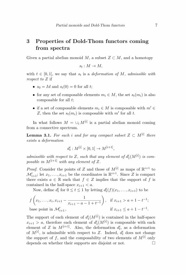
Lemma 3.1. For each i and for any compact subset Z ⊂ M [i] thereexists a deformation
dit : M[i] × [0, 1] → M [i+1],
admissible with respect to Z, such that any element of di1(M[i]) is com-
posable in M [i+1] with any element of Z.
Proof. Consider the points of Z and those of M [i] as maps of Ri+1 toM′
i+1; let x1, . . . , xi+1 be the coordinates in Ri+1. Since Z is compactthere exists a ∈ R such that f ∈ Z implies that the support of f iscontained in the half-space xi+1 < a.
Now, define dit for 0 ≤ t ≤ 1 by letting dit(f)(x1, . . . , xi+1) to be
f
(x1, . . . , xi, xi+1 −
1
xi+1 − a− 1 + t−1
), if xi+1 > a+ 1− t−1;
base point in M′i+1 , if xi+1 ≤ a+ 1− t−1.
The support of each element of di1(M[i]) is contained in the half-space
xi+1 > a, therefore each element of di1(M[i]) is composable with each
element of Z in M [i+1]. Also, the deformation dit, as a deformationof M [i], is admissible with respect to Z. Indeed, dit does not changethe support of f , and the composability of two elements of M [i] onlydepends on whether their supports are disjoint or not.

8 Jacob Mostovoy
Lemma 3.2. Let I be the abelian monoid whose elements are points of[0, 1] with the sum of two numbers being their maximum. For each ithere is homomorphism of partial monoids
hi : M[i] → I
which only vanishes at zero, and a deformation
ui : M[i] × [0, 1] → M [i],
which is constant on the set hi = 1, decreases the value of hi strictlymonotonically on the set hi < 1, at the value of the parameter t < 1 is ahomeomorphism and at t = 1 retracts the subspace hi < 1/4 into the basepoint. Moreover ui and the restriction of ui+1 to M [i] are homotopic.
Proof. First we define inductively a collection of functions li : M′i →
[0, 1]. The space M′0 is a point and we set li to be equal to zero on it.
Assume that we have already defined the function lk. By construction,the space M′
k+1 is the mapping cylinder of the map ΣM′k → Mk+1
induced by the structure map of the spectrum M. Consider the reducedsuspension ΣM′
k as the product M′k × [−1, 1] with the identifications
(∗, s) ∼ (x, 1) ∼ (x,−1)
for all x ∈ M′k and s ∈ [−1, 1], and let τ be the cylinder coordinate,
which is equal to 0 on ΣM′k and to 1 on Mk+1. Then we set lk+1 = 1
if τ = 1 and
lk+1((x, s), τ) = max (min (lk(x), 2− 2|s|), τ)
for (x, s) ∈ ΣM′k and τ < 1.
In the same vein, define a collection of retractions wi : M′i× [0, 1] →
M′i. Let qt with t ∈ [0, 1] be a continuous family of continuous mono-
tonic functions from [0, 1] to itself such that
• qt(0) = 0 and qt(a) = a for all t and a ≥ 1/2;
• qt is strictly monotonic for t < 1, and q1(a) = 0 for a < 1/4;
• qt(a) > qt′(a) for all 0 < a < 1/2 and t < t′.
Partial monoids and Dold-Thom functors 9
Also define r(τ, l) as
r(τ, l) =
0 if 0 ≤ τ ≤ 1/2, 0 ≤ l ≤ 1/2;
2τ − 1 if 1/2 < τ ≤ 1, 0 ≤ l ≤ 1/2;
2τ l − τ if 0 ≤ τ ≤ 1/2, 1/2 < l ≤ 1;
−2τ l + 3τ + 2l − 2 if 1/2 < τ ≤ 1, 1/2 < l ≤ 1.
Then, assuming that we have already defined wk, we set wk+1 to beconstant on Mk+1 and on the set τ < 1 we define
(wk+1)t((x, s), τ) =(((wk)t(x), 1− qt(1− s)), tr(τ, l) + (1− t)τ
)
if s ≥ 0, and
(wk+1)t((x, s), τ) =(((wk)t(x),−1 + qt(1 + s)), tr(τ, l) + (1− t)τ
)
for negative s.It is verified directly that wi is constant on the set li = 1, decreases
the value of li strictly monotonically on the set li < 1, at the value ofthe parameter t < 1 is a homeomorphism and at t = 1 deforms thesubspace li < 1/4 into the base point. Now, define the function hi onM [i] on a map α : Ri → M′
i as the maximal value of hi α and thedeformation ui of M
[i] as that induced by the deformation wi. It is clearthat the conditions of the lemma are then satisfied.
Lemma 3.3. The set π0(M) is an abelian group with the addition in-duced by the partial addition in M .
Proof. It is sufficient to notice that if points of M are thought of asmaps of R to Ωi−1M′
i for some i, an inverse to a map γ in π0M will begiven by γ(C − t) for sufficiently big C.
For a space X let M<a>[X] ⊂ M [X] be the subset of configurationswhose coefficients are composable with a ∈ M .
Lemma 3.4. The inclusion of M<a>[X] into M [X] induces isomor-phisms on all homotopy groups. Moreover, if
∑(xi,mi) ∈ M<a>[X],
the map
M<a+∑
mi>[X] → M<a>[X]
given by summing with∑
(xi,mi), is also a weak homotopy equivalence.

10 Jacob Mostovoy
Proof. We first need to show that the image of any map f of a finite cellcomplex Y into M [X] can be deformed into M<a>[X]. Assume that theimage of f is contained in M [i][X]. Then, applying the deformation ditfrom Lemma 3.1, with Z = a, to all the labels of the configurationsf(y), where y ∈ Y , we get a homotopy of f to a map of Y into M<a>[X].
In order to establish the second claim, for each mi choose mi in sucha way that the class of mi is inverse to that of mi in π0M and so thatthe sum a+
∑mi +
∑mi is defined.
It is then easy to see that adding∑
(xi,mi) and then∑
(xi, mi)to a configuration in M<a+
∑mi+
∑mi>[X] is homotopic to the natural
inclusion
M<a+∑
mi+∑
mi>[X] → M<a>[X].
Since all the natural inclusions between the spacesM<a>[X] for differenta are homotopy equivalences, it follows that the map in the statementof the lemma is surjective on the homotopy groups. Replacing in thisargument a by a+
∑mi we see that the map
M<a+∑
mi+∑
mi>[X] → M<a+∑
mi>[X],
given by adding∑
(xi, mi), is also surjective on homotopy and thisproves the lemma.
4 Quasifibrations of Dold-Thom functors
The proof of Theorem 2.3.1 is based on the original argument of Doldand Thom [4], see also [1, 5]. We have the following fact:
Proposition 4.1. Let M be a partial monoid coming from a connectivespectrum. If X is a cell complex and A ⊂ X is a subcomplex, the mapM [X] → M [X/A] is a quasifibration with the fibre M [A].
The rest of this section is dedicated to the proof of this statement.Note that we do not require A to be connected.
We shall need the following criterion for quasifibrations. Let p :E → B be a map which is quasifibration over B′ ⊂ B. Assume thatfor any compact C ⊂ B there is a homotopy ft of the inclusion mapi : C → B to a map C → B′, which maps C∩B′ to B′ for all t. Further,suppose that for any compact C ⊆ p−1(C) there is a homotopy ft of the

Partial monoids and Dold-Thom functors 11
inclusion map C → E to a map C → p−1(B′) which maps C ∩ p−1(B′)to p−1(B′) for all t, and such that
p ft = ft p.
Moreover, assume that ft and ft are well-defined up to homotopy.Take a point b ∈ B and b ∈ p−1(b). Then we have two paths: from
b to b′ ∈ B′ and from b ∈ p−1(b) to b′ ∈ p−1(b′), the latter covering theformer. This gives a map of the homotopy groups
πi(p−1(b), b) → πi(p
−1(b′), b′).
Lemma 4.2. Assume that all the above maps of homotopy groups of thefibres are isomorphisms for all i ≥ 0. Then the map p is a quasifibration.
This lemma is a version of Hilfssatz 2.10 of [4] and the proof is,essentially, the same.
We denote by p the projection map
X → X/A
and by π the induced map
M [X] → M [X/A].
We shall prove by induction on n that the map π is a quasifibrationover Mn[X/A]. This, by Satz 2.15 of [4] (or Theorem A.1.17 of [1]) willimply that π is a quasifibration over the whole M [X/A].
Assume that π is a quasifibration over Mn−1[X/A]. According toSatz 2.2 of [4] (or Theorem A.1.2 of [1]) it is sufficient to prove that π isa quasifibration over Mn[X/A] −Mn−1[X/A], over a neighbourhood ofMn−1[X/A] in Mn[X/A] and over the intersection of this neighbourhoodwith Mn[X/A]−Mn−1[X/A].
It will be convenient to speak of delayed homotopies. A delayedhomotopy is a map ft : A × [0, 1] → B such that for some ε > 0 wehave ft = f0 when t ≤ ε. A map p : E → B is said to have the delayedhomotopy lifting property if it has the homotopy lifting property withrespect to all delayed homotopies of finite cell complexes into B. It isclear that a map that has the delayed homotopy lifting property is aquasifibration.
Lemma 4.3. Let B be an arbitrary subspace of Mn[X/A]−Mn−1[X/A].The map π, when restricted to π−1(B), has the delayed homotopy liftingproperty.
12 Jacob Mostovoy
Proof. Letft : Z × [0, 1] → B
be a delayed homotopy of a finite cell complex Z into B, such thatft = f0 for t ≤ ε, and let
f0 : Z → π−1(B)
be its lifting at t = 0.Notice thatMn[X/A]−Mn−1[X/A] can be thought of as the subspace
of Mn[X] consisting of configurations of n distinct points, all outsideA and with non-trivial labels. Therefore, we can think of B as of asubspace of Mn[X].
Define g : Z → M [X] as the difference
g(z) = f0(z)− f0(z).
The map g is well-defined, continuous and its image belongs to M [A].Since Z is compact, the image of f0 belongs to M [i][X] for some i; itfollows that the coefficients of g(z) are composable with the coefficientsof f0(z) in M [i] for all z ∈ Z.
Lemma 3.1 guarantees the existence of a deformation dit of M [i]
inside M [i+1] such that each point in di1(M[i]) is composable in M [i+1]
with each point in the image of Z × [0, 1] under ft. There is an induceddeformation of M [i][A] which we also denote by dit.
Define the homotopy gt : Z → M [A] as dktε−1 g for 0 ≤ t < ε andas dk1 g for ε ≤ t ≤ 1. Lemma 3.1 implies that gt is well-defined and iscomposable with ft for all t. Consider the map ft = ft+gt : Z → M [X].By construction, it lifts ft.
It remains to see that the map π is a quasifibration over some neigh-bourhood of Mn−1[X/A].
Recall from Lemma 3.2 that there is a homomorphism of partialmonoids
M [i] → I
which sends a map α to the maximal value of hi α. It gives rise to amap
vi : M[i]n [X] → In[X].
If X and A are cell complexes, let ∆ be the subspace of In[X] con-sisting of configurations which either contain a point of A, or have lessthan n points. It is not hard to show that In[X] is a cell complex and
Partial monoids and Dold-Thom functors 13
∆ is a subcomplex. In particular, ∆ is a strong deformation retract ofits neighbourhood U ⊂ In[X]. Let
dt : In[X]× [0, 1] → In[X]
be the deformation that retracts U to ∆. We can assume that dt is ahomeomorphism for all t < 1. Then dt can be lifted to a deformation
Dt : M[i]n [X]× [0, 1] → M [i]
n [X],
that retracts the open subset v−1i (U) to the subspace v−1
i (∆) ⊂ M[i]n [X],
which consists of configurations which either contain a point of A, orhave less than n points.
Now, by construction, there exists a deformation
Dt : M[i]n [X/A]× [0, 1] → M [i]
n [X/A],
such thatDt π = π Dt
for all t. In particular, Dt retracts the open neighbourhood π(v−1i (U))
of M[i]n−1[X/A] onto M
[i]n−1[X/A].
Let V be the union of all the neighbourhoods π(v−1i (U)) for all i in
M [X/A]. Then V is open in M [X/A] and it follows from Lemma 3.4that the projection π−1(V ) → V satisfies the conditions of Lemma 4.2.
5 On the spectrum M [S]
5.1 The spectrum M [S] and the proof of Theorem 2.3.1.
Proposition 4.1 with X = Dn and A = ∂Dn gives the quasifibration
M [Sn−1] → M [Dn] → M [Sn].
The spaceM [Dn] is contractible, and therefore, we have weak homotopyequivalences M [Sn−1] ΩM [Sn] and the spaces M [Si] for i ≥ 0 forman Ω-spectrum which we denote by M [S].
More generally, given X, the cofibration X → CX → ΣX givesrise to a weak homotopy equivalence M [X] ΩM [ΣX], and given aninclusion map i : A → X, the cofibration A → Cyl(i) → X ∪i CA givesrise to an exact sequence
. . . π∗M [A] → π∗M [X] → π∗M [X ∪i CA] → π∗−1M [A] → . . . .

14 Jacob Mostovoy
Here CX is the cone on X and Cyl(i) is the cylinder of the map i. Sinceπ∗M [X] is, clearly, a homotopy functor, this means that the groupsπ∗M [X] form a reduced homology theory.
There is a natural transformation of the homology with coefficientsin M [Si] to π∗M [X], induced by the obvious map
M [Si] ∧X → M [Si ∧X]
that sends(∑
mizi, x)to
∑mi(zi, x):
limi→∞
πk+i
(M [Si] ∧X
)→ lim
i→∞πk+iM [Si ∧X] = πkM [X].
If X is a sphere, the Freudenthal Theorem implies that this is an iso-morphism. Hence, π∗M [X] coincides as a functor, on connected cellcomplexes, with the homology with coefficients in M [S].
5.2 The weak equivalence of M [S] and M.
We shall first construct a weak homotopy equivalence between the infi-nite loop spaces of the spectra M and M [S] and then show that thereexists an inverse to this equivalence, which is induced by a map of spec-tra. This will establish Theorem 2.3.1.
Let I be the interval [−1/2, 1/2]. By Proposition 4.1 the map I → S1
which identifies the endpoints of I induces a quasifibration M [I] →M [S1] with the fibre M Ω∞M∞.
Since M [I] is contractible, it follows that M is weakly homotopyequivalent to ΩM [S1]; the weak equivalence is realized by the map ψthat sends m ∈ M to the loop (parameterized by I) whose value at thetime t ∈ I is the configuration consisting of one point with coordinate−t and label m.
Let us now define the map of spectra Φ, inverse to the above weakequivalence ψ.
For n > 0 identify Sn with the n-dimensional cube
In = [−1/2, 1/2]n ⊂ Rn,
modulo its boundary. Fix a homeomorphism of the interior of In withRn, say, by sending each coordinate uk to tanπuk. Think of a point inM [Sn] as of a sum
∑(xα,mα) where xα ∈ In and mα are maps from In
to M′n. Assume that the maps mα(−xα) are composable as maps from
some Ri to M′n+i. Then their sum is a well-defined point of M′
n whichdoes not depend on i. We set Φn(
∑(xα,mα)) to be equal to this sum.

Partial monoids and Dold-Thom functors 15
The map Φn : M [Sn] → M′n is only partially defined, but this
problem can be circumvented as follows. Let M∗[Sn] ⊂ M [Sn] be thesubspace consisting of the configurations
∑(xα,mα) such that for some
i the points mα(qα) ∈ Ω′iM′n+i are composable (that is, have disjoint
supports in Ri) for any choice of the qα ∈ In.The spaces M∗[Sn] form a sub-spectrum M∗[S] of M [S]. Indeed,
the structure map of M [S] sends∑
(xα,mα) ∈ M [Sn] to the loop t →∑((xα, t),mα), where t ∈ I. The map Φn is well-defined on M∗[Sn]. If
we define the map Φ0 simply as ΩΦ1, it is clear from the constructionthat Φ0 ψ is the identity map on M0. The proof will be finished assoon as we prove the following
Proposition 5.2.1. The inclusion map M∗[Sn] → M [Sn] is a weakhomotopy equivalence for all n > 0.
Proof. Define M∗k [S
n] as M∗[Sn] ∩ Mk[Sn]. It sufficient to prove that
the inclusion M∗k [S
n] → Mk[Sn] is a weak homotopy equivalence for all
k.For k = 1 this inclusion is the identity map. Also, for k > 1 the map
(1) M∗k [S
n]/M∗k−1[S
n] → Mk[Sn]/Mk−1[S
n]
is a weak homotopy equivalence. Indeed, take a map
f : Sj → Mk[Sn]/Mk−1[S
n]
and let us show that the labels of the points in each configuration inthe image of f can be pushed away from each other, thus deforming theimage of f into M∗
k [Sn]/M∗
k−1[Sn].
By forgetting the labels in the configurations we get a map
(Sj − f−1(∗)) → Bk(Sn)
to the configuration space of k distinct particles in Sn. Without lossof generality we can assume that the boundary of Sj − f−1(∗) is acollared (for instance, smooth) hypersurface in Sj , so that this mapgives rise to a bundle ξ of k-element sets over the compactification C ofSj − f−1(∗). In turn, this bundle of sets gives rise to a k-vector bundleη whose fibre is spanned by the elements of the corresponding fibre of ξ.Since C is compact, η can be considered as a subbundle of some trivialbundle. What this means is that there exists an N such that given aconfiguration in the image of f we can assign a unit vector in some RN
16 Jacob Mostovoy
to each of its points so that the vectors assigned to all the points aremutually orthogonal.
Now, the image of f is contained in M[i]k [Sn]/M
[i]k−1[S
n] for somei. We can treat the labels of the configurations in the image of f aselements of
M [i+N ] = ΩiΩNM′i+N ,
and write them as functions m(x, y) with x ∈ Ri and y ∈ RN . For z ∈ Cwrite f(z) =
∑(qα,mα) where qα ∈ Sn and mα ∈ M [i+N ], and define
ft(z) as
ft(z) =∑
(qα,mα(x, y + tvα)),
where vα are the orthogonal vectors associated to the points qα of theconfiguration f(z). Then for t sufficiently large, the image of ft will liein M∗
k [Sn]/M∗
k−1[Sn].
The subspacesMk−1[Sn] ⊂ Mk[S
n] andM∗k−1[S
n] ⊂ M∗k [S
n] are not,strictly speaking, neighbourhood deformation retracts, but each of thesesubspaces has a neighbourhood such that the map of any compact intothis neighbourhood can be retracted onto the subspace. This is sufficientto claim that the fact that the maps (1) are weak homotopy equivalencesimplies that the inclusion M∗
k [Sn] → Mk[S
n] induce isomorphisms inhomology. The fundamental groups of these two spaces are easily seen tobe abelian for k > 1, just as in the case of the usual symmetric products,and, hence, this inclusion is a weak homotopy equivalence.
Acknowledgement
I would like to thank Ernesto Lupercio for conversations that pro-vided the motivation for this paper, and to Norio Iwase, Dai Tamakiand Peter Teichner for pointing out useful references. I am also gratefulto Max-Planck-Institut fur Mathematik, Bonn for hospitality during thestay at which this paper was written.
Jacob MostovoyDepartamento de Matematicas,Centro de Investigacion y deEstudios Avanzados del IPN,Apartado Postal 14-740,07000 Mexico, [email protected]

Partial monoids and Dold-Thom functors 17
References
[1] Aguilar M.; Gitler S.; Prieto C., Algebraic Topology from a Ho-motopical Viewpoint, Springer-Verlag, 2002.
[2] Anderson D. W., Chain functors and homology theories., Sympos.Algebraic Topology (1971), Lect. Notes Math. 249 1971, 1-12.
[3] Bousfield A. K.; Friedlander E. M., Homotopy theory of Γ-spaces,spectra, and bisimplicial sets., Geom. Appl. Homotopy Theory,II, Proc. Conf., Evanston (1977), Lect. Notes Math. 658 1978,80-130.
[4] Dold A.; Thom R., Quasifaserungen und unendliche symmetrischeProdukte., Ann. Math. 67 (1958), 239-281.
[5] Hatcher A., Algebraic Topology,. Cambridge University Press,Cambridge, 2002.
[6] Kuhn N., The McCord model for the tensor product of a space anda commutative ring spectrum., Categorical decomposition tech-niques in algebraic topology., Birkhauser, Basel, 2004.
[7] May J. P., Categories of spectra and infinite loops spaces., Lect.Notes Math. 99 1969, 448-479.
[8] McCord M. C., Classifying spaces and infinite symmetric prod-ucts., Trans. Am. Math. Soc. 146 (1969), 273-298.
[9] Voevodsky V., A1-homotopy theory. Proceedings of the Interna-tional Congress of Mathematicians, Vol. I Berlin (1998), Doc.Math. Extra Vol. I 1998, 579-604.
[10] Segal G., Configuration-spaces and iterated loop-spaces., Inven-tiones Math. 21 (1973), 213–221.
[11] Segal G., Categories and cohomology theories., Topology 13(1974), 293–312.
[12] Segal G., K-homology theory and algebraic K-theory., K-TheoryOper. Algebr., Proc. Conf. Athens/Georgia (1975), Lect. NotesMath. 575 1977, 113-127.
[13] Schwanzl R.; Vogt R.M., E∞-spaces and injective Γ-spaces,Manuscripta Math. 61 (1988), 203–214.

18 Jacob Mostovoy
[14] Shimakawa K., Configuration spaces with partially summable la-bels and homology theories., Math. J. Okayama Univ. 43 (2001),43-72.

Morfismos, Vol. 17, No. 1, 2013, pp. 19–39
Algebra C∗ generada por operadores de Toeplitz
con sımbolos discontinuos en el espacio de
ocinomranamgreB ∗
Maribel Loaiza Carmen Lozano
Resumen
Sea una curva simple suave en el disco unitario complejo D.arbeglaledniklaCedarbeglalesomaidutseojabartetsenE C∗
edoicapselenenautcaeuqztilpeoTedserodareporopadarenegedocinomranamgreB D, cuyos sımbolos son funciones continuas
en D \ . El resultado principal e inesperado es que el espectro deaetnatsnocnoicnufanuseolobmısoyucztilpeoTedrodareponu
.dadiunitnocsidedolugnaledednepedsozort
2010 Mathematics Subject Classification: 31A05,32A10,32A36,47L80.Keywords and phrases: funcion armonica, espacios de Berman, algebrasC∗, proyecciones de Bergman, anti-Bergman, operador de Toeplitz.
noiccudortnI1
arbeglaleraidutseseojabartetseedovitejbolE C∗ generada por opera-oiratinuocsidledocinomranamgreBedoicapseleneztilpeoTedserod
complejo. Existen numerosos trabajos sobre operadores de Toeplitz consımbolo continuo y continuo a trozos actuando en el espacio de Bergmandel disco unitario, entre ellos [15].
Con respecto a operadores de Toeplitz actuando en el espacio deserodareposololudom,euqartseumedes]7[ne,ocinomranamgreB
∗Trabajo basado en la tesis de Carmen Lozano, dirigida por Maribel Loaiza, pre-nocsaicneiCneaırtseaMedodarglednoicnetboalarapotisiuqeromocadatnes
.0102edoreneed52leNPI-VATSEVNICledsacitametaMnedadilaicepse
19
20 Maribel Loaiza y Carmen Lozano
compactos, el algebra C∗ generada por los operadores de Toeplitz, consımbolo continuo es isomorfa al algebra de funciones continuas en lafrontera de D. Un hecho muy conocido es que este mismo resultadoes valido cuando los operadores de Toeplitz actuan en el espacio deBergman.
En general, el comportamiento de los operadores de Toeplitz de-pende del espacio donde estos actuan. Uno de los resultados importantesque se tienen es que el ındice de un operador de Toeplitz actuando enel espacio de Bergman depende del numero de vueltas que su sımboloda al cero. Por otro lado, si estos operadores actuan en el espacio deBergman armonico, tienen siempre ındice cero como se demuestra en[7]. Mas aun, en este trabajo, demostramos que si el sımbolo de unoperador de Toeplitz es continuo a trozos, su ındice es tambien cero.
Otra de las diferencias importantes entre los operadores de Toeplitzactuando en el espacio de Bergman con respecto a los mismos actuandoen el espacio de Bergman armonico es el exhibido en el Corolario 3.9.En este corolario se muestra que el espectro de un operador de Toeplitzcon sımbolo continuo a trozos depende del angulo de discontinuidad enla frontera del disco.
En este trabajo se toma como base los artıculos [6] y [9]. En elprimer artıculo se estudia el algebra C∗ generada por los operadoresde multiplicacion por funciones continuas a trozos, la proyeccion deBergman y la proyeccion anti-Bergman y; en el segundo, se estudia elalgebra C∗ generada por los operadores de multiplicacion por funcionescontinuas a trozos y la proyeccion armonica.
2 Preliminares
A lo largo de este trabajo D denotara al disco unitario abierto en el planocomplejo C, es decir, D = z ∈ C : |z| < 1 y T denotara su frontera∂D = z ∈ C : |z| = 1. Para z = x+ iy, dm(z) = 1
πdxdy es la medidade Lebesgue normalizada en D. El espacio de Bergman A2(D) del discoD es el espacio de funciones analıticas de L2(D) y A2(D) = f : f ∈A2(D), el espacio anti-Bergman, es el espacio de todas las funcionesanti-analıticas de L2(D). Los espacios de Bergman y anti-Bergman sonsubespacios cerrados de L2(D) = L2(D, dm) y por lo tanto son espaciosde Hilbert.
Operadores de Toeplitz con sımbolos discontinuos 21
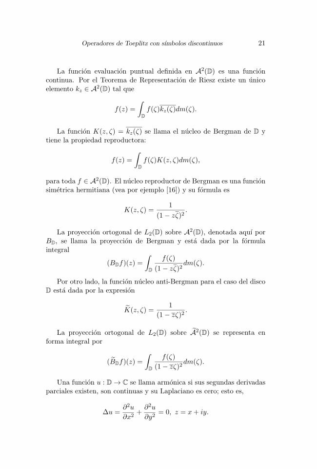
La funcion evaluacion puntual definida en A2(D) es una funcioncontinua. Por el Teorema de Representacion de Riesz existe un unicoelemento kz ∈ A2(D) tal que
f(z) =
∫
Df(ζ)kz(ζ)dm(ζ).
La funcion K(z, ζ) = kz(ζ) se llama el nucleo de Bergman de D ytiene la propiedad reproductora:
f(z) =
∫
Df(ζ)K(z, ζ)dm(ζ),
para toda f ∈ A2(D). El nucleo reproductor de Bergman es una funcionsimetrica hermitiana (vea por ejemplo [16]) y su formula es
K(z, ζ) =1
(1− zζ)2.
La proyeccion ortogonal de L2(D) sobre A2(D), denotada aquı porBD, se llama la proyeccion de Bergman y esta dada por la formulaintegral
(BDf)(z) =
∫
D
f(ζ)
(1− zζ)2dm(ζ).
Por otro lado, la funcion nucleo anti-Bergman para el caso del discoD esta dada por la expresion
K(z, ζ) =1
(1− zζ)2.
La proyeccion ortogonal de L2(D) sobre A2(D) se representa enforma integral por
(BDf)(z) =
∫
D
f(ζ)
(1− zζ)2dm(ζ).
Una funcion u : D → C se llama armonica si sus segundas derivadasparciales existen, son continuas y su Laplaciano es cero; esto es,
∆u =∂2u
∂x2+
∂2u
∂y2= 0, z = x+ iy.
22 Maribel Loaiza y Carmen Lozano
El espacio de Bergman armonico b2(D) es el conjunto de todas lasfunciones armonicas complejas u en D para las cuales
‖u‖2 =(∫
D|u(ζ)|2 dm(ζ)
)1/2
< ∞.
El espacio b2(D) es un subespacio cerrado de L2(D) y por lo tanto esun espacio de Hilbert. Ademas cada evaluacion puntual es un funcionallineal acotado en b2(D); vea por ejemplo [1]. Por lo tanto existe unaunica funcion R(z, ·) en b2(D) la cual satisface la propiedad:
u(z) =
∫
Du(ζ) R(z, ζ) dm(ζ), (z ∈ D)
para todo u ∈ b2(D). El nucleo reproductor armonico R(z, ·) es realy simetrico. Tambien podemos ver que b2(D) ∩ L∞(D) es denso enb2(D). Sea Q la correspondiente proyeccion ortogonal del espacio deHilbert L2(D) en b2(D). La proyeccion de Bergman armonica Q tienela representacion
(1) Q = BD + BD + T,
donde T es el operador unidimensional dado por la formula
(Tf)(z) = −∫
Df(w) dm(w).
Para una funcion a ∈ L∞(D) definimos el operador de Toeplitz consımbolo a, Ta : b2(D) → b2(D) mediante la formula
Ta(u) = Q(au).
A continuacion enunciamos algunas propiedades, cuyas demostracionesson inmediatas, que cumplen los operadores de Toeplitz en el espaciode Bergman armonico.
Teorema 2.1. Sean a, b ∈ L∞(D) y α, β ∈ C, entonces
(i) ‖Ta‖2 ≤ ‖a‖∞,
(ii) Tαa+βb = αTa + βTb,
(iii) T ∗a = Ta.

Operadores de Toeplitz con sımbolos discontinuos 23
Actualmente existen varias tecnicas de localizacion en teorıa de ope-radores. Uno de los trabajos pioneros en esta area fue realizado porSimonenko ([12]) en 1965. En este trabajo se introduce la nocion deoperadores localmente equivalentes y se desarrolla lo que posteriormentese conocerıa como principio local de Simonenko. En el estudio de estecampo surge el desarrollo de varios principios locales, entre ellos, el prin-cipio local de Douglas-Varela ([14]). En el se establece la representacionde un algebra C∗ como el espacio de secciones continuas de un haz C∗.
Una propiedad muy importante de los operadores de Toeplitz consımbolo continuo, actuando en b2(D), es que el conmutador y el semi-conmutador de cada par de este tipo de operadores es compacto (veapor ejemplo [2], [5] y [10]). Esto nos permite utilizar el principio localde Douglas-Varela, usando como subalgebra central al algebra generadapor los operadores de Toeplitz con sımbolo continuo. Como es usualC(D) denota al algebra de las funciones continuas en D.
Teorema 2.2 ([2], [10]). Sean a, b ∈ C(D), entonces el conmutador[Ta, Tb] = TaTb − TbTa y el semiconmutador [Ta, Tb) = Tab − TaTb soncompactos en b2(D).
El teorema que presentamos a continuacion es muy importante en elestudio del algebra C∗ generada por operadores de Toeplitz. Pues nosdice que el ideal de operadores compactos contiene a los operadores deToeplitz cuyo sımbolo se anula en la frontera del disco unitario complejo.
Teorema 2.3 ([2], [10]). Si a ∈ C(D), entonces Ta es compacto enb2(D) si y solo si la restriccion a|T ≡ 0.
El siguiente resultado describe la relacion que hay entre los sımbolosarmonicos de dos operadores de Toeplitz que conmutan.
Teorema 2.4 ([3]). Sean u, v ∈ b2(D) funciones no constantes. En-tonces TuTv = TvTu en b2(D) si y solo si v = αu+ β con α, β ∈ C.
2.1 Las proyecciones de Bergman y anti-Bergman en elsemiplano superior.
Consideremos el semiplano superior Π con la medida de area dz = dxdy,z = x + iy. Como es usual L2(Π) denota al espacio de todas las fun-ciones medibles cuadrado integrables en Π. El correspondiente espaciode Bergman de todas las funciones analıticas de L2(Π) se denotara por

24 Maribel Loaiza y Carmen Lozano
A2(Π). La proyeccion ortogonal de L2(Π) en A2(Π) se denota por BΠ.Analogamente, A2(Π) denota al subespacio de L2(Π) formado por lasfunciones anti-analıticas y BΠ a la proyeccion ortogonal de L2(Π) sobreA2(Π), llamada proyeccion anti-Bergman (ver [13]). En coordenadaspolares tenemos la descomposicion:
(2) L2(R2, dxdy) = L2(R+, rdr)⊗ L2(T, dω),
donde dω es la medida de longitud de arco en T.
D
Figura 1: La curva en el disco unitario D.
Sea una curva simple suave a trozos en el disco unitario cerrado D.Sea t0 el punto donde la curva intersecta a T. Denotemos por PC(D, )al conjunto de todas las funciones a(z), continuas en D \ que tienenlımite por la derecha y por la izquierda en t0, estos seran denotados pora+(t0) y a−(t0) respectivamente.
Sin perdida de generalidad podemos suponer que t0 = −1. Conside-remos el operador Wφ : L2(D) → L2(Π), dado por la regla de correspon-dencia
(3) (Wφf)(z) = f φ−1(z) φ−1z (z),
donde φ(z) = i z+11−z transforma a D en Π y φz =
∂φ∂z . Es facil comprobar
que Wφ es un operador unitario, autoadjunto y por tanto una isometrıa

Operadores de Toeplitz con sımbolos discontinuos 25
lineal. Consideremos tambien el operador unitario V : L2(Π) → L2(Π)definido por V = h(z)I, donde
(4) h(z) =
(z + i
z − i
)2
.
Proposicion 2.5 ([6], [11]). BD es unitariamente equivalente a BΠ yBD es unitariamente equivalente a V ∗BΠV.
Para una funcion operador-valuada
L : R → B(L2(T)),λ → L(λ),
denotaremos por I ⊗λ L(λ) al operador en B (L2(R)⊗ L2(T)) dado porla formula
[(I ⊗λ L(λ))f ](λ, t) = [L(λ)f(λ, ·)](t), (λ, t) ∈ R× T.
El siguiente teorema proporciona una descomposicion de BΠ y BΠ
en terminos de operadores unidimensionales. Denotaremos por T+ a lainterseccion T ∩Π.
Teorema 2.6 ([8]). Los operadores BΠ y BΠ son unitariamente equiva-lentes a las familias de operadores I⊗λB(λ) e I⊗λB(λ) respectivamente.Donde para cada λ ∈ R los operadores B(λ), B(λ) ∈ B(L2(T+)) son lasproyecciones ortogonales sobre los espacios unidimensionales generadospor las funciones
gλ(t) =
√2λ
1−e−2πλ tiλ−1, λ = 0,
t−1√π, λ = 0,
gλ(t) =
√2λ
e2πλ−1t−iλ+1, λ = 0,
t√π, λ = 0,
respectivamente, con t ∈ T. Mas aun, 〈gλ, gλ〉 = 0 y B(λ)B(λ) = 0,para todo λ ∈ R.
2.2 El algebra de Toeplitz
Denotaremos por K al espacio formado por todos los operadores com-pactos en el espacio de Bergman armonico b2(D). Sea T (C(D)) el alge-bra C∗ generada por los operadores de Toeplitz en el espacio de Bergman

26 Maribel Loaiza y Carmen Lozano
armonico con sımbolo en C(D). El algebra de Toeplitz T (C(D)) esirreducible y contiene al ideal K (vea por ejemplo [7]). Ademas cadaelemento en T (C(D)) es de la forma Tv +K, donde K es un operadorcompacto y v ∈ b2(D).
En [7] Kunyu Guo y Dechao Zheng probaron el siguiente resultado.
Teorema 2.7. La sucesion
0 −→ K i−−→ T (C(D)) j−−→ C(T) −→ 0
es una sucesion exacta corta; esto es, el algebra cociente T (C(D))/K esisometricamente ∗-isomorfa a C(T), donde i es la inclusion y j es lafuncion que transforma Ta +K en la restriccion a|T.
El teorema anterior muestra similitudes entre T (C(D)) en el espa-cio de Bergman armonico y en el espacio de Bergman, pues el mismoresultado se cumple cuando los operadores actuan en el espacio deBergman A2(D). Sin embargo el ındice de Fredholm de un operador deToeplitz actuando en b2(D) es siempre cero contrastando con el corres-pondiente ındice de Fredholm de un operador actuando en el espaciode Bergman A2(D), cuyo ındice depende del numero de vueltas que lafuncion sımbolo le da al origen.
3 El algebra generada por los operadores deToeplitz con sımbolo continuo a trozos
Sea TPC = T (PC(D, )) el algebra C∗ generada por los operadores deToeplitz en el espacio de Bergman armonico con sımbolos en PC(D, ).Al contener al algebra T (C(D)), el algebra TPC es irreducible y contieneal ideal K. Denotaremos por π a la proyeccion natural
π : T (PC(D, )) → TPC := T (PC(D, ))/K.
Describiremos el algebra de Calkin de T (PC(D, )) utilizando el Prin-cipio Local de Douglas-Varela (para detalles vea [13]).
En la representacion (1) para la proyeccion Q, T es un operadorcompacto de modo que, salvo una perturbacion compacta, la proyeccionQ es la suma de las proyecciones BD y BD.

Operadores de Toeplitz con sımbolos discontinuos 27
Para a ∈ L∞(D), denotamos por Ma : L2(D) → L2(D) al operadorde multiplicacion
Ma(f) = af.
El siguiente resultado nos permite usar al algebra π(T (C(D)) =T (C(D)) como subalgebra central conmutativa del algebra T (PC(D, )).
Proposicion 3.1. Sea a ∈ C(D) y b ∈ L∞(D), entonces el conmutador[Ta, Tb] = TaTb − TbTa es compacto.
Demostracion. Los operadores BD y BD son operadores de tipo local(ver [4]), por lo que Q = BD+ BD+T es tambien de tipo local. Esto es,Q conmuta con los operadores de multiplicacion por funciones continuasen D modulo un operador compacto. Por otra parte, tenemos
TaTb − TbTa = QMaQMb −QMbQMa
= QMaMb −QMbQMa +K
= QMbMa −QMbQMa +K
= QMb[I −Q]Ma +K
= QMbHa +K,
donde K ∈ K. El operador de Hankel Ha : b2(D) → L2(D) es compactopues su sımbolo es continuo en D (ver [5]), entonces [Ta, Tb] es compacto.
Denotaremos por A a la imagen en TPC de un operador A en elalgebra T (PC(D, )). Por el Teorema 2.7 T (C(D))/K es isomorfo aC(T), por lo que su espacio de ideales maximales es isomorfo a T.
Sea J(t) el ideal maximal en C(T) correspondiente al punto t ∈ T,es decir,
J(t) = aI +K : a ∈ C(T), a(t) = 0 .
Denotaremos por J(t) = J(t) · TPC al ideal bilateral cerrado de TPC
generado por J(t). De forma analoga al caso de sımbolos continuos,TPC(t) = TPC/J(t) representa al algebra de Calkin de TPC y πt : TPC →TPC(t) la proyeccion natural.
Al algebra TPC(t) la llamamos el algebra local de TPC en el puntot. Dos operadores A1 y A2 en TPC(D, ) se llamaran localmente equiva-lentes en t si
πt(A1) = πt(A2),
28 Maribel Loaiza y Carmen Lozano
donde A1 (respectivamente A2) es la imagen de A1 (A2) bajo π.
La descripcion de las algebras locales TPC(t) se descompone en doscasos: los puntos t ∈ T \ −1 y t = −1.
3.1 Algebras Locales del algebra TPC
El resultado que mostramos a continuacion nos proporciona la descrip-cion de las algebras locales en los puntos del conjunto T \ −1.
Teorema 3.2. El algebra local de TPC en el punto t0 ∈ T \ −1 esisomorfa a C.
Demostracion. El operador de multiplicacion por una funcion a(t)I eslocalmente equivalente a a(t0)I en el punto t0. Dado que BD+BD+K esla identidad en TPC , el operador de Toeplitz con sımbolo a es localmenteequivalente en t0 a a(t0)I. El isomorfismo entre TPC(t0) y C esta dadopor (
BD + BD
)a(t)I → a(t0).
Supondremos que la curva es tal que bajo transformaciones de
Mobius, se transforma en un rayo que sale del origen en el semiplanosuperior. Sin perdida de generalidad podemos suponer que divide aldisco D en dos regiones que denotaremos por D1 y D2.
Utilizando la Proposicion 2.5 y el hecho de que la funcion h(z),definida en la formula (4), es tal que h(0) = 1 obtenemos el siguientelema.
Lema 3.3. Sea t0 = −1. Entonces el algebra local TPC(t0) es isomorfa
al algebra generada por los operadores(BΠ + BΠ
)WφχDjW
∗φ , j = 1, 2,
donde Wφ esta dado por la ecuacion (3).
Para una funcion a(z) ∈ PC(D) sea
(5) a+(z) = limz→z0z∈D1
a(z) y a−(z) = limz→z0z∈D2
a(z).
Consideremos los operadores y las transformaciones definidas en (3) y(4) y sean L = φ(), Π1 = φ(D1), Π2 = φ(D2). Ası,
Π1 = z ∈ Π : 0 < arg z < θ,

Operadores de Toeplitz con sımbolos discontinuos 29
Π2 = z ∈ Π : θ < arg z < π,donde θ es el angulo que forma la recta L con el eje X del semiplanosuperior Π.
D
D2
D1
t
θ
φ Π φ()
Π1 = φ(D1)θ
Figura 2: La transformacion de Mobius φ envıa al disco D en el semi-plano superior Π.
Lema 3.4. El algebra local en un punto t = −1 es isomorfa al algebragenerada por
(6) (BΠ + BΠ)χΠjI, j = 1, 2,
donde χΠj denota la funcion caracterıstica del conjunto Πj , j = 1, 2.
Demostracion. Se sigue del hecho que localmente en cero V , definidoen (4), es equivalente al operador identidad y del Lema 3.3.
Comenzaremos pues a describir el algebra C∗ generada por los ope-radores
(BΠ + BΠ)χΠjI, j = 1, 2.
De acuerdo al Teorema 2.6, esta ultima algebra es isomorfa al algebra C∗
generada por las funciones((I ⊗λ B(λ) + I ⊗λ B(λ))χiI
)λ∈R
,
actuando en L2(R+)⊗L2(T+) y donde χi es la funcion caracterıstica delarco T+ ∩ Πi, i = 1, 2. Observemos que χ1 es la funcion caracterısticadel arco determinado por el angulo θ, es decir,
(7) χ1I = χθI, χ2I = I − χθI,

30 Maribel Loaiza y Carmen Lozano
donde
(8) χθ(t)I =
1 si t ∈ [0, θ),0 si t ∈ [θ, π].
Mas aun, dado que B(λ) y B(λ) son proyecciones ortogonales entresı Q(λ) := B(λ) + B(λ) es una proyeccion. El Teorema 2.6 nos indicaque Q(λ) es la proyeccion bidimensional de L2(T+) sobre el subespacioH de L2(T+) generado por gλ y gλ. Esta proyeccion esta dada por
(9) Q(λ)f = 〈f, gλ〉gλ + 〈f, gλ〉gλ,
para f ∈ L2(T+) y L2(T+) = H ⊕H⊥.
Denotemos por Uλ al algebra C∗ generada por Q(λ) y las proyec-ciones χθI e I − χθI. Para analizar Uλ denotaremos por M1 y M2 alas imagenes de las proyecciones χθI e I − χθI respectivamente. Ob-servemos que Mj ∩H = 0 y Mj ⊂ H⊥. Consideremos el subespaciocerrado de L2(T+)
(10) H0 = (H⊥ ∩M1)⊕ (H⊥ ∩M2)
y M = H⊥0 . Descompongamos L2(T+) en la suma directa
(11) L2(T+) = H0 ⊕M.
Tenemos que H ⊂ M. Consideremos las restricciones de las proyec-ciones Q(λ), χθI e I − χθI al espacio M definidas por
Q′ = Q(λ) |M, P1 = χθI |M, P2 = (I − χθI) |M .
Dado que χθI e I − χθI suman la identidad en L2(T+), tenemos queP1+P2 = I ′, donde I ′ es la identidad en M. Por otra parte, como Mj ⊂H⊥ se sigue que todas las restricciones Pj son no triviales. Ademas
ImP1 = χθI(M) = M1 ∩M.
De forma analoga ImP2 = M2 ∩ M. Ahora, si y ∈ Mj ∩ M entoncesy ∈ Pj(M) por lo que Mj ∩ M ⊂ Pj(M). Haciendo M ′
j = Mj ∩ Mtenemos que
(12) M = M ′1 ⊕M ′
2.
Operadores de Toeplitz con sımbolos discontinuos 31
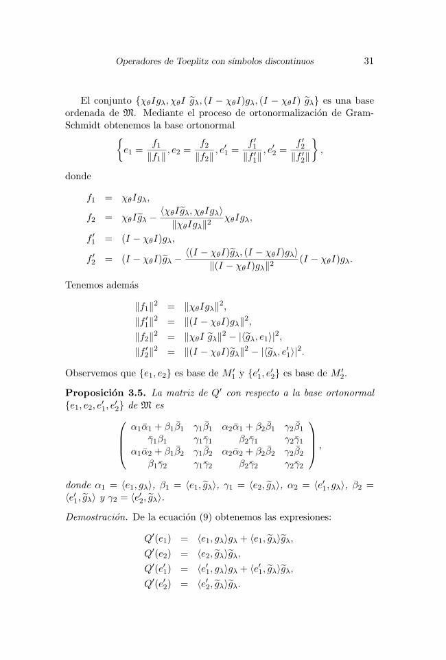
El conjunto χθIgλ, χθI gλ, (I − χθI)gλ, (I − χθI) gλ es una baseordenada de M. Mediante el proceso de ortonormalizacion de Gram-Schmidt obtenemos la base ortonormal
e1 =
f1‖f1‖
, e2 =f2‖f2‖
, e′1 =f ′1
‖f ′1‖
, e′2 =f ′2
‖f ′2‖
,
donde
f1 = χθIgλ,
f2 = χθIgλ − 〈χθIgλ, χθIgλ〉‖χθIgλ‖2
χθIgλ,
f ′1 = (I − χθI)gλ,
f ′2 = (I − χθI)gλ − 〈(I − χθI)gλ, (I − χθI)gλ〉
‖(I − χθI)gλ‖2(I − χθI)gλ.
Tenemos ademas
‖f1‖2 = ‖χθIgλ‖2,‖f ′
1‖2 = ‖(I − χθI)gλ‖2,‖f2‖2 = ‖χθI gλ‖2 − |〈gλ, e1〉|2,‖f ′
2‖2 = ‖(I − χθI)gλ‖2 − |〈gλ, e′1〉|2.
Observemos que e1, e2 es base de M ′1 y e′1, e′2 es base de M ′
2.
Proposicion 3.5. La matriz de Q′ con respecto a la base ortonormale1, e2, e′1, e′2 de M es
α1α1 + β1β1 γ1β1 α2α1 + β2β1 γ2β1γ1β1 γ1γ1 β2γ1 γ2γ1
α1α2 + β1β2 γ1β2 α2α2 + β2β2 γ2β2β1γ2 γ1γ2 β2γ2 γ2γ2
,
donde α1 = 〈e1, gλ〉, β1 = 〈e1, gλ〉, γ1 = 〈e2, gλ〉, α2 = 〈e′1, gλ〉, β2 =〈e′1, gλ〉 y γ2 = 〈e′2, gλ〉.
Demostracion. De la ecuacion (9) obtenemos las expresiones:
Q′(e1) = 〈e1, gλ〉gλ + 〈e1, gλ〉gλ,Q′(e2) = 〈e2, gλ〉gλ,Q′(e′1) = 〈e′1, gλ〉gλ + 〈e′1, gλ〉gλ,Q′(e′2) = 〈e′2, gλ〉gλ.
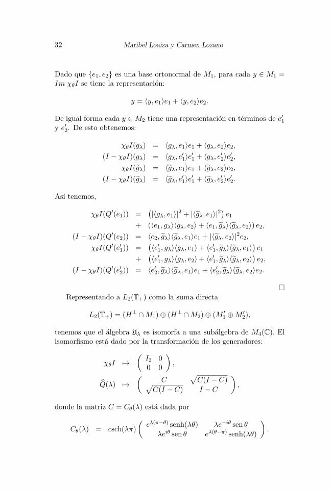
32 Maribel Loaiza y Carmen Lozano
Dado que e1, e2 es una base ortonormal de M1, para cada y ∈ M1 =Im χθI se tiene la representacion:
y = 〈y, e1〉e1 + 〈y, e2〉e2.
De igual forma cada y ∈ M2 tiene una representacion en terminos de e′1y e′2. De esto obtenemos:
χθI(gλ) = 〈gλ, e1〉e1 + 〈gλ, e2〉e2,(I − χθI)(gλ) = 〈gλ, e′1〉e′1 + 〈gλ, e′2〉e′2,
χθI(gλ) = 〈gλ, e1〉e1 + 〈gλ, e2〉e2,(I − χθI)(gλ) = 〈gλ, e′1〉e′1 + 〈gλ, e′2〉e′2.
Ası tenemos,
χθI(Q′(e1)) =
(|〈gλ, e1〉|2 + |〈gλ, e1〉|2
)e1
+ (〈e1, gλ〉〈gλ, e2〉+ 〈e1, gλ〉〈gλ, e2〉) e2,(I − χθI)(Q
′(e2)) = 〈e2, gλ〉〈gλ, e1〉e1 + |〈gλ, e2〉|2e2,χθI(Q
′(e′1)) =(〈e′1, gλ〉〈gλ, e1〉+ 〈e′1, gλ〉〈gλ, e1〉
)e1
+(〈e′1, gλ〉〈gλ, e2〉+ 〈e′1, gλ〉〈gλ, e2〉
)e2,
(I − χθI)(Q′(e′2)) = 〈e′2, gλ〉〈gλ, e1〉e1 + 〈e′2, gλ〉〈gλ, e2〉e2.
Representando a L2(T+) como la suma directa
L2(T+) = (H⊥ ∩M1)⊕ (H⊥ ∩M2)⊕ (M ′1 ⊕M ′
2),
tenemos que el algebra Uλ es isomorfa a una subalgebra de M4(C). Elisomorfismo esta dado por la transformacion de los generadores:
χθI →(
I2 00 0
),
Q(λ) →(
C√
C(I − C)√C(I − C) I − C
),
donde la matriz C = Cθ(λ) esta dada por
Cθ(λ) = csch(λπ)
(eλ(π−θ) senh(λθ) λe−iθ sen θ
λeiθ sen θ eλ(θ−π) senh(λθ)
).
Operadores de Toeplitz con sımbolos discontinuos 33
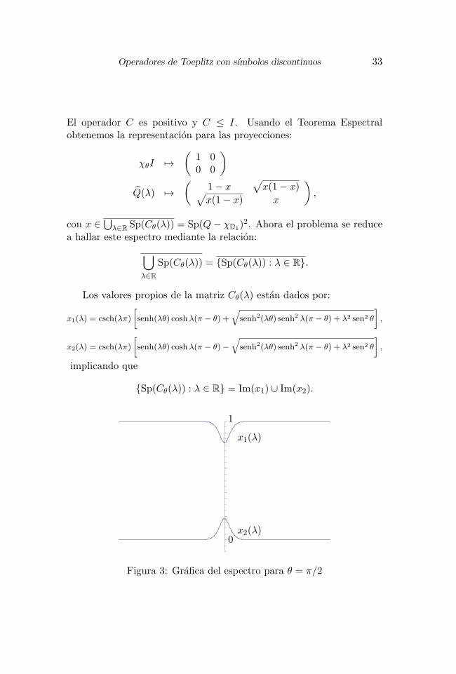
El operador C es positivo y C ≤ I. Usando el Teorema Espectralobtenemos la representacion para las proyecciones:
χθI →(
1 00 0
)
Q(λ) →(
1− x√
x(1− x)√x(1− x) x
),
con x ∈⋃
λ∈R Sp(Cθ(λ)) = Sp(Q− χD1)2. Ahora el problema se reduce
a hallar este espectro mediante la relacion:
⋃λ∈R
Sp(Cθ(λ)) = Sp(Cθ(λ)) : λ ∈ R.
Los valores propios de la matriz Cθ(λ) estan dados por:
x1(λ) = csch(λπ)
[senh(λθ) coshλ(π − θ) +
√senh2(λθ) senh2 λ(π − θ) + λ2 sen2 θ
],
x2(λ) = csch(λπ)
[senh(λθ) coshλ(π − θ)−
√senh2(λθ) senh2 λ(π − θ) + λ2 sen2 θ
],
implicando que
Sp(Cθ(λ)) : λ ∈ R = Im(x1) ∪ Im(x2).
1
0
x1(λ)
x2(λ)
Figura 3: Grafica del espectro para θ = π/2
34 Maribel Loaiza y Carmen Lozano
1
0
x1(λ)
x2(λ)
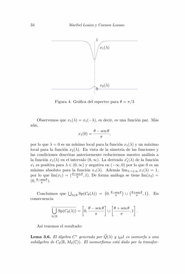
Figura 4: Grafica del espectro para θ = π/3
Observemos que x1(λ) = x1(−λ), es decir, es una funcion par. Masaun,
x1(0) =θ − sen θ
π,
por lo que λ = 0 es un mınimo local para la funcion x1(λ) y un maximolocal para la funcion x2(λ). En vista de la simetrıa de las funciones ylas condiciones descritas anteriormente reduciremos nuestro analisis ala funcion x1(λ) en el intervalo (0,∞). La derivada x′1(λ) de la funcionx1 es positiva para λ ∈ (0,∞) y negativa en (−∞, 0) por lo que 0 es unmınimo absoluto para la funcion x1(λ). Ademas limλ→±∞ x1(λ) = 1,por lo que Im(x1) = ( θ+sen θ
π , 1). De forma analoga se tiene Im(x2) =
(0, θ−sen θπ ).
Concluimos que⋃
λ∈R Sp(Cθ(λ)) =(0, θ−sen θ
π
)∪(θ+sen θ
π , 1). En
consecuencia
⋃λ∈R
Sp(Cθ(λ)) =
[0,
θ − sen θ
π
]∪[θ + sen θ
π, 1
].
Ası tenemos el resultado:
Lema 3.6. El algebra C∗ generada por Q(λ) y χθI es isomorfa a unasubalgebra de Cb(R,M2(C)). El isomorfismo esta dado por la transfor-
Operadores de Toeplitz con sımbolos discontinuos 35
macion de los generadores:
Q(λ) →(
1 00 0
),
χθI →(
1− x√
x(1− x)√x(1− x) x
),
con x ∈ [0, θ−sen θπ ] ∪ [ θ+sen θ
π , 1].
Teorema 3.7. El algebra local de TPC en el punto t0 = −1 es isomorfaal algebra
C(Sp(Q− χD1)
2).
El isomorfismo esta dado por la transformacion de los generadores:
Qa(z)IQ → a+(t0)(1− x) + a−(t0)x,
con x ∈ ∆ := [0, θ−sen θπ ] ∪ [ θ+sen θ
π , 1].
3.2 Descripcion del algebra TPC
Denotemos por T la compactificacion de T \ −1. Bajo esto, al puntot = −1 le corresponde un par de puntos en T, t+1 y t−1 , ordenados en
direccion positiva. El conjunto T coincide con el conjunto de idealesmaximales del algebra TPC .
Para pegar las diferentes algebras locales consideraremos los dife-rentes puntos en la frontera de D. El Teorema 3.7 muestra que TPC(t)es isomorfa al algebra C([0, θ−sen θ
π ] ∪ [ θ+sen θπ , 1]), para t = −1.
Para un operador compacto K, consideramos el generador del alge-bra TPC : A = (BD + BD)a(z)I +K. Usando el Teorema 3.7 podemosdefinir
A(x) = a+(t)(1− x) + a−(t)x
donde x ∈ [0, θ−sen θπ ] ∪ [ θ+sen θ
π , 1]. Entonces tenemos
A(0) = a+(t), A(1) = a−(t).
Sea ϑ la funcion que identifica los puntos de ∆ con los puntos de T,dada por la formula
ϑ(0) = t+1 ,
ϑ(1) = t−1 .
36 Maribel Loaiza y Carmen Lozano
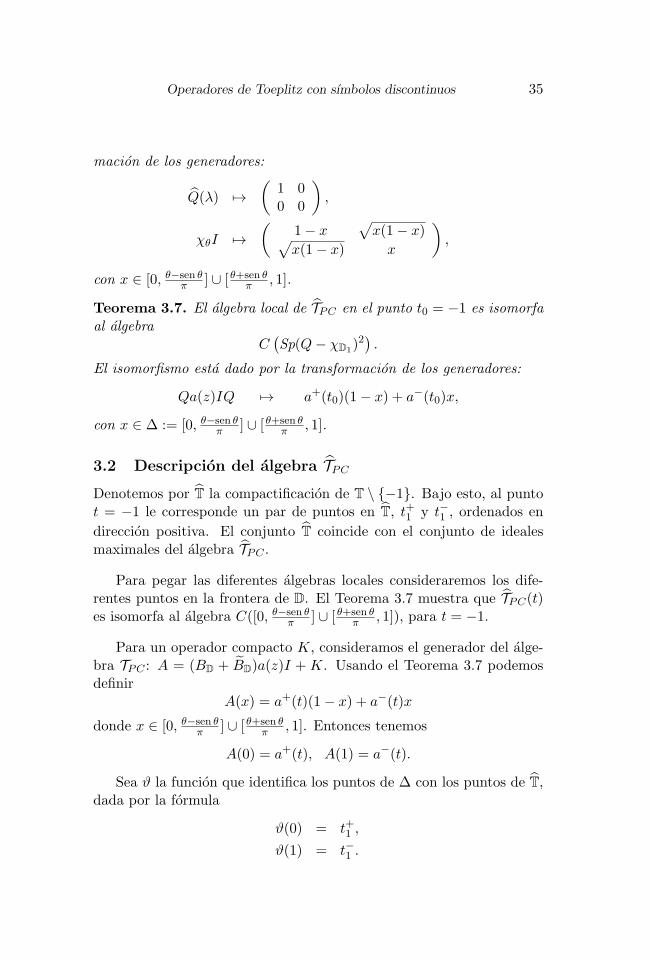
Figura 5: Curva Γ = ∆ ∪ϑ T
Sean σ1 ∈ C(T) y σ2 ∈ C(∆). Denotemos por S al algebra de todoslos pares (σ1, σ2) que satisfacen las condiciones:
limx→t−1
σ2(x) = σ1(ϑ(0))(13)
limx→t+1
σ2(x) = σ0(ϑ(1))(14)
La norma en el algebra S esta determinada como sigue
‖σ‖ = max
supT
|σ1(t)|, sup∆
‖σ2(x)‖
.
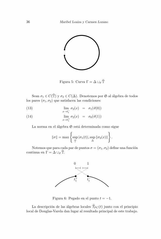
Notemos que para cada par de puntos σ = (σ1, σ2) define una funcioncontinua en Γ = ∆ ∪ϑ T.
t+1 t−1
0 1
Figura 6: Pegado en el punto t = −1.
La descripcion de las algebras locales TPC(t) junto con el principiolocal de Douglas-Varela dan lugar al resultado principal de este trabajo.

Operadores de Toeplitz con sımbolos discontinuos 37
Teorema 3.8. El algebra de Calkin TPC del algebra C∗ T (PC(D, )) esisomorfa e isometrica a C(Γ). El isomorfismo sym : TPC → C(Γ) estadado por la transformacion de los generadores del algebra TPC :
sym : A = (BD + BD)a(z)I +K →
a(t), t ∈ T,a+(t)x+ a−(t)(1− x), x ∈ ∆, t = −1,
donde a±(t) son los lımites definidos por la formula (5).
Finalmente, consideremos el conjunto de operadores de Fredholm deTPC y que denotaremos por Fred(TPC).
Corolario 3.9. El ındice de cada operador en Fred(TPC) es cero.
Mostraremos esto mediante el diagrama:
Fred(TPC)
Ind
π G(TPC)ind G(TPC)/G0(TPC)
ΨZ
Por un lado, G(TPC) = G(C(Γ)) y este consiste de las funciones con-tinuas en Γ que no se anulan en Γ. Calcularemos ahora la componenteconexa de la identidad en G(C(Γ)), es decir, G0(C(Γ)). Para esto ob-servemos que cada funcion a ∈ C(Γ) es homotopica a la identidad.Entonces G0(Γ) = G(C(Γ)) y en consecuencia
G(TPC)/G0(TPC) = 0.
Por lo tanto el ındice de Fredholm de cada operador es cero.
Maribel LoaizaDepartamento de Matematicas,CINVESTAV-IPN,Apartado Postal 14-740,07000, Mexico, [email protected]
Carmen LozanoDepartamento de Matematicas,CINVESTAV-IPN,Apartado Postal 14-740,07000, Mexico, [email protected]
Referencias
[1] Axler S.; Bourdon P.; Ramey W., Harmonic Function Theory,Graduate Text in Mathematics 137, Springer, New York, 1992.
38 Maribel Loaiza y Carmen Lozano
[2] Choe B. R.; Lee Y. J.; Na K., Toeplitz operators on harmonicBergman spaces, Nagoya Math. J. 174 (2004), 165–186.
[3] Choe B. R.; Lee Y. J., Commuting Toeplitz operators on the har-monic Bergman spaces, Michigan Math. J. 46 (1999), 163–174.
[4] Dzhuraev A., Methods of Singular Integral Equations, PitmanMonographs and Surveys in Pure and Applied Mathematics 60,Longman Scientific and Technical, 1992.
[5] Jovovic M., Compact Hankel operators on harmonic Bergmanspaces, Integral Equations Operator Theory 22 (1995), 295–304.
[6] Karlovich Y. I.; Pessoa L., Algebras generated by the Bergmanand anti-Bergman projections and by multiplications by piecewisecontinuous functions, Integral Equations Operator Theory, 52:2(2005), 219–270.
[7] Guo K.; Zheng D., Toeplitz algebra and Hankel algebra on theharmonic Bergman space, J. Math. Anal. Appl. 276 (2002), 213–230.
[8] Loaiza M., Algebras generated by the Bergman projection and op-erators of multiplication by piecewise continuous functions, Inte-gral Equations Operator Theory 46 (2003), 215–234.
[9] Loaiza M., On the algebra generated by the harmonic Bergmanprojection and operators of multiplication by piecewise continuousfunctions, Bol. Soc. Mat. Mexicana 10:2 (2004), 179–193.
[10] Miao J., Toeplitz operators on harmonic Bergman spaces, IntegralEquations Operator Theory 27:4 (1997), 426–438.
[11] Ramırez de Arellano E.; Vasilevski N., Bargmann projection,three-valued functions and corresponding Toeplitz operators, Con-temp. Math. 212 (1998), 185–196.
[12] Simonenko I. B., A new general method to study linear opera-tor equations of the singular integral equation type, II, Izv. Akad.Nauk SSSR, Ser. Math., 29 (1965), 757–782.
[13] Vasilevski N. L., On Toeplitz operators with piecewise continuoussymbols on the Bergman space, Operator Theory: Advances andApplications 170 (2007), 229–248.

Operadores de Toeplitz con sımbolos discontinuos 39
[14] Vasilevski N. L., C*-bundle approach to a local principle, Re-porte Interno 363, Departamento de Matematicas, CINVESTAVdel I.P.N., Mexico, 2005.
[15] Vasilevski N. L., Commutative Algebras of Toeplitz Operators onthe Bergman Space, Birkhauser Basel, 2008.
[16] Zhu K., Operator Theory in Function Spaces, Marcel Dekker Inc.,New York and Basel, 1990.


Morfismos, Vol. 17, No. 1, 2013, pp. 41–65
Ideals, varieties, stability, colorings and
combinatorial designs ∗
zonuMreivaJ 1 slogaSuileF 2 Charles J. Colbourn 3
Abstract
A combinatorial design is equivalent to a stable set in a suitablychosen Johnson graph, whose vertices correspond to all k-sets thatcould be blocks of the design. In order to find maximum stable setsof a graph G, two ideals are associated with G, one constructed
nizsavoLybdetroperenodnaalumrofssuartS-nikztoMehtmorfconnection with the stability polytope. These ideals are shown tocoincide and form the stability ideal of G. Graph stability idealsbelong to a class of 0-1 ideals. These ideals are shown to be radical,and therefore have a strong structure.
Stability ideals of Johnson graphs provide an algebraic char-acterization that can be used to generate Steiner triple systems.Two different ideals for the generation of Steiner triple systems,and a third for Kirkman triple systems, are developed. The lastof these combines stability and colorings.
2010 Mathematics Subject Classification: 05B07,13P10.Keywords and phrases: computational algebraic geometry, Grobner ba-sis, combinatorial designs, Steiner triple systems, binary ideals.
1 Introduction
Our main objective is to establish links between design theory and al-eW.sesabrenborGdnaslaedifoesuehthguorhtyrtemoegciarbeg
∗The authors thank ABACUS-CINVESTAV, CONACyT grant EDOMEX-2011-C01-165873.
1The content of this paper is part of the Ph.D. thesis of the first author working-SEVNICfoscitamehtaMfotnemtrapeDehttaslogaSuileFfonoisivrepusehtrednu
TAV. Supported by CONACyT and CINVESTAV.2Partially supported by SNI under contract number 7008 and CINVESTAV.3Partially supported by DOD grant N00014-08-1-1069.
41

42 J. Munoz, F. Sagols and C. J. Colbourn
concentrate on Steiner triple systems because they are simple designswith well known properties; however, the algebraic geometry techniquesthat we use can be easily translated to other designs.
Let us start defining the fundamental objects and concepts fromdesign theory, graph theory and algebraic geometry with which we work.A maximum packing by triples (MPT or MPT(n)) of order n > 0 is amaximum cardinality set of triples in 0, . . . , n−1 such that every pairi, j ∈ 0, . . . , n−1 is in at most one triple. MPTs exist for every n ≥ 3.When n ≡ 1, 3 (mod 6), an MPT(n) is a Steiner triple system (STSor STS(n)); in this case, every 2-subset of elements appears in exactlyone triple.
All graphs considered here are simple. Let v, , and i be fixedpositive integers with v ≥ ≥ i. Let Ω be a cardinality v set. Definea graph J(v, , i) as follows. The vertices of J(v, , i) are the -subsetsof Ω, two -subsets being adjacent if their intersection has cardinality i.Therefore, J(v, , i) has
(v
)vertices and it is a regular graph with valency(
i
)(v−−i
). For v ≥ 2, graphs J(v, , − 1) are Johnson graphs [11].
One of the main methods that we use to characterize MPT(n)s con-sists of finding stable sets (or independent sets) in J(n, 3, 2). A stableset S of a graph G is a subset of vertices in V (G) containing no pair ofadjacent vertices in G. The maximum size of a stable set in G is thestability number of G, denoted by α(G).
The stability polytope of a n-vertex graph G is the convex hull of(x0, . . . , xn−1) | xi = 1 or xi = 0 and i ∈ V (G) | xi = 1 is a stableset of G.
We also use vertex colorings. A λ vertex coloring (or coloring forshort) of a graph G (where λ is a positive integer) is a function c :V (G) → 1, . . . , λ such that (v, w) ∈ E(G) if and only if c(v) = c(w).The minimum value of λ for which a λ coloring of G exists is the chro-matic number of G, denoted by χ(G).
We introduce some algebraic structures. For k a field, k[x] = k[x1,. . . , xn] is the polynomial ring in n variables. A subset I ⊂ k[x1, . . . , xn]is an ideal of k[x1, . . . , xn] if it satisfies 0 ∈ I; if f, g ∈ I, then f + g ∈ I;and if f ∈ I and h ∈ k[x1, . . . , xn] then hf ∈ I. When f1, . . . , fs arepolynomials in k[x1, . . . , xn] we set
〈f1, . . . , fs〉 =
s∑
i=1
hifi
∣∣∣∣h1, . . . , hs ∈ k[x1, . . . , xn]
.
Then 〈f1, . . . , fs〉 is an ideal (see [7]) of k[x1, . . . , xn], the ideal gener-

Ideals and combinatorial designs 43
ated by f1, . . . , fs. One remarkable result, the Hilbert Basis Theorem [7],establishes that every ideal I ⊂ k[x1, . . . , xn] has a finite generating set.
The monomials in k[x] are denoted by xa = xa11 xa22 · · ·xann ; they areidentified with lattice points a = (a1, . . . , an) in Nn, where N is the set ofnonnegative integers. A total order ≺ on Nn is a term order if the zerovector is the unique minimal element, and a ≺ b implies a+ c ≺ b+ cfor all a,b, c ∈ Nn.
Given a term order ≺, every nonzero polynomial f ∈ k[x] has aunique initial monomial, denoted by in≺(f). If I is an ideal in k[x],then its initial ideal is the monomial ideal in≺(I) := 〈in≺(f) : f ∈ I〉.
The monomials that do not lie in in≺(I) are standard monomials.A finite subset G ⊂ I is a Grobner basis for I with respect to ≺ ifin≺(I) is generated by in≺(g) : g ∈ G. If no monomial in this set isredundant, the Grobner basis is unique for I and ≺, provided that thecoefficient of in≺(g) in g is 1 for each g ∈ G.
A finite subset U ⊂ I is a universal Grobner basis if U is a Grobnerbasis of I with respect to all term orders ≺ simultaneously.
A field k is algebraically closed if for every polynomial f ∈ k[x] inone variable, the equation f(x) = 0 has a solution in k. Every field kis contained in a field k that is algebraically closed and such that everyelement of k is the root of a nonzero polynomial in one variable withcoefficients in k. This field is unique up to isomorphism, and is thealgebraic closure of k.
Given a subset S ⊆ k[x1, . . . , xn], the variety Vk(S) in kn is
Vk(S) = (a1, . . . , an) ∈ kn | f(a1, . . . , an) = 0 for all f ∈ S.
If I = 〈f1, . . . , fs〉 ⊆ k[x1, . . . , xn] then
Vk(I) = (a1, . . . , an) ∈ kn | fi(a1, . . . , an) = 0, 1 ≤ i ≤ s= Vk(f1, . . . , fs).
One of the most remarkable results in algebraic geometry is the follow-ing.
Theorem 1.1 (Weak Hilbert Nullstellensatz [12]). Let I be an ideal con-tained in k[x1, . . . , xn]. Then Vk(I) = ∅ if and only if I = k[x1, . . . , xn].
We may use this theorem to demonstrate that some designs do notexist, by proving that they correspond to varieties of ideals whose re-duced Grobner basis is 1, or equivalently that I = k[x1, . . . , xn] and,by the weak Hilbert Nullstellensatz, the variety is empty.
44 J. Munoz, F. Sagols and C. J. Colbourn
These are the fundamental objects employed, and more specific def-initions are introduced as needed. With the exception of the idealsintroduced in Section 7, we use the field of rational numbers. When analgebraic closed field is needed, the complex numbers are used instead.Computations for Grobner basis ideals are done in Macaulay 2 [9].
The paper is organized as follows. In Section 2 an ideal to gener-ate stable sets based on the Motzkin-Strauss formula [16] is first intro-duced. Then, a general ideal introduced by Lovasz [15] which has beenextensively used for the generation of stable sets in graphs is described.Both ideals are examples of 0-1 ideals, a recently introduced class hav-ing combinatorial applications beyond stability [19]. These ideals areshown to be radical, and consequently the equality of the two idealsis established. Section 3 introduces basic properties of stability ideals.In Section 4 the stability ideal of J(n, 3, 2) is determined and used tobuild MPTs; difficulties to solve the equations involved are explored,and potential means to generate MPTs with restrictions are examined.In particular, a modification of the stability ideal of J(n, 3, 2) is shownto generate anti-Pasch MPTs. Section 5 introduces two new ideals togenerate MPTs that use colorings instead of stable sets. Section 6 in-troduces an ideal to generate Kirkman triple systems that employs amixture of techniques based on stable sets and on colorings. Section7 explores parametric generation of MPTs. Finally, in section 8 someconcluding remarks are made.
2 Stable sets and ideals
Combinatorial and algebraic aspects of the stable set problem have beenextensively studied. One of the most interesting connections is given bythe Motzkin-Strauss explicit formula for α(G) [16]:
Theorem 2.1. Let G = (V,E) be a graph. Then
1− 1
α(G)= max
2
∑i,j /∈E
xixj
∣∣∣∣∑
i∈V (G)
xi = 1, xi ≥ 0
.(1)
The Motzkin-Strauss formula enables one to determine part of thestructure of the stability polytope, and consequently to prove severalresults in extremal graph theory, including Turan’s Theorem. In (1),α(G) is determined by an optimization problem which at first sightmight be solved by Lagrange multipliers. Unfortunately the objective
Ideals and combinatorial designs 45
function reaches its maximum at the feasible region boundary and outof this region it is unbounded. We can circumvent this problem bysquaring each variable to get a different version of the Motzkin-Straussformula that still yields α(G):
1− 1
α(G)= max
2
∑i,j /∈E
y2i y2j
∣∣∣∣∑
i∈V (G)
y2i = 1
.(2)
Lagrange multipliers can be used for (2). Make the objective func-tion’s gradient equal to a multiplier λ times the restriction function’sgradient to obtain the system of equations:
4yi∑
j∈V (G)|i,j /∈E
y2j = 2λyi for each i ∈ V (G),(3)
∑i∈V (G)
y2i = 1.
This system has several solutions that do not maximize (2). Lovasz[15] characterizes the set of maximum solutions for (1): Any vector xmaximizes the right hand side if and only if x has a stable set as supportand if xi = 0 for some i ∈ V (G) then xi = 1/α(G). Let y be an optimalsolution to (2) such that yj ≥ 0 for every j ∈ V (G). From (3), if yi = 0then
4α(G)− 1
α(G)√
α(G)= 4
1√α(G)
α(G)− 1
α(G)= 4yi
∑j∈V (G)|i,j /∈E
y2j
= 2λyi = 2λ1√α(G)
So, a solution of (3) is a maximum of the objective function in (2)
if and only if λ = 2α(G)−1α(G) . If we substitute this value in (3), substitute
zi = y2i α(G), and introduce the equations zi(zi − 1) = 0 to restrict thevalues of zi to 0 or 1, then we transform (3) into
zi(zi − 1) = 0 for each i ∈ V (G),

46 J. Munoz, F. Sagols and C. J. Colbourn
zi(∑
j∈V (G)|i,j /∈E
zj − α(G) + 1) = 0 for each i ∈ V (G),(4)
∑i∈V (G)
zi − α(G) = 0.
This yields:
Proposition 2.2. The graph G has stability number at least e if andonly if the following zero-dimensional system of equations
x2i − xi = 0 for every node i ∈ V (G),
xi(∑
j∈V (G)|i,j /∈E
xj − e+ 1) = 0 for each i ∈ V (G),(5)
n∑i=1
xi − e = 0,
has a solution. The vector x is a solution of (5) if and only if the supportof x is a stable set.
The ideal generated by the polynomials in (5) is the Motzkin-Straussideal of G, denoted by MS(G).
A second approach was introduced by Lovasz [15].
Proposition 2.3 (Lovasz). The graph G has stability number at leaste if and only if the zero-dimensional system of equations
x2i − xi = 0 for every node i ∈ V (G),
xixj = 0 for every edge i, j ∈ E(G),(6)n∑
i=1
xi − e = 0,
has a solution. Vector x is a solution of (6) if and only if the supportof x is a stable set.
Proof. If there exists some solution x to these equations, the identitiesx2i − xi = 0 ensure that all variables take values only in 0, 1. Theset S = i|xi = 1 is stable because equations xixj = 0 guarantee thatthe end points of any edge in E(G) cannot belong simultaneously to S.Finally, the cardinality of S is e by the last equation.
The ideal generated by the polynomials in (6) is the stability ideal ofG, denoted by S(G). As Lovasz [15] explains, solving (6) appears to be

Ideals and combinatorial designs 47
hopeless but he uses S(G) to write alternative proofs of several knownrestrictions on the stability polytope.
A quick comparison of S(G) and MS(G) demonstrates that theideals are close; actually their generators only differ in the polynomialsdefined in terms of E(G). However the generators of both ideals containthe polynomials x2i − xi for i ∈ V (G). This condition confers on thema strong structure that we can generalize by introducing a bigger classof ideals containing them.
Let I be an ideal in k[x1, . . . , xn]. Then I is a 0-1 ideal if x21 −x1, x
22 − x2, . . . , x
2n − xn ⊂ I. Ideals S(G) and MS(G) are 0-1 ideals.
Our objective now is to prove that 0-1 ideals are radical, with the con-sequence that the Motzkin-Strauss and stability ideals are the same forany graph G.
For a polynomial f ∈ k[x1, . . . , xn] write f = pv11 pv22 · · · pvmm where thepolynomials pv11 pv22 · · · pvmm are irreducible. Polynomial f∗ = p1p2 · · · pmis the square free part of f . Polynomial f is square free if and only iff = f∗.
IfM is an additive group, for a natural number n and an element a ofM , na denotes the n-ple sum a+ · · ·+a of a (the addition of a, n times).Under the notation, we define the characteristic of a ring k, denotedchart(k) as follows. Consider the set D = n ∈ N|na = 0 for every a ∈k. If D is empty, then the characteristic of k is defined to be zero,otherwise, the least number in D is defined to be the characteristic ofk. The next result is due to A. Seidenberg.
Lemma 2.4. [2, pages 341-342, 8.2] Let k be a field and let I be azero-dimensional ideal of k[x1, . . . , xn], and assume that for 1 ≤ i ≤ n,I contains a polynomial fi ∈ k[xi] with gcd(fi, f
′i) = 1. Then I is an
intersection of finitely many maximal ideals. In particular, I is thenradical.
Proposition 2.5. [1] Let I be a zero-dimensional ideal and G be thereduced Grobner basis for I with respect to the lex term order with x1 <x2 < · · · < xn. Then we can order g1, . . . , gt such that g1 contains onlythe variable x1, g2 contains only the variables x1 and x2 and lp(g2) is apower of x2, g3 contains only the variables x1, x2 and x3 and lp(g3) isa power of x3, and so forth until gn.
Here lp(g) stands for the leader power of the polynomial g.
Theorem 2.6. Let k a field and I a 0-1 ideal in k[x1, . . . , xn] then I isa radical ideal.
48 J. Munoz, F. Sagols and C. J. Colbourn
Proof. Let G be the reduced Grobner basis for I. If 1 ∈ G, by Theorem1.1 I = k[x1, . . . , xn], and hence I =
√I. Now we consider the case
when I is zero-dimensional. Since for each i = 1, . . . , n, I contains theunivariate polynomial fi = x2i − xi satisfying gcd(fi, f
′i) = gcd(x2i −
xi, 2xi − 1) = 1 the result follows from Lemma 2.4.
Theorem 2.7 (Strong Hilbert Nullstellensatz). I(Vk(I)) =√I for all
ideals I of k[x1, . . . , xn].
As a consequence, two ideals I and J correspond to the same variety(Vk(I) = Vk(J)) if and only if
√I =
√J .
Proposition 2.8. For G a graph, S(G) = MS(G).
Proof. By Theorem 2.6 S(G) and MS(G) are both radical. By Propo-sitions 2.2 and 2.3 these two ideals correspond to the same variety.Finally, by Theorem 2.7 both ideals coincide.
Note that Proposition 2.8 is valid for all field k.
This gives two names and two ways to designate the same ideal, sohenceforth the terminology of stability ideal and S(G) is used. All ex-tremal graph theory results implied from the Motzkin-Strauss formulaand those about the stability polytope can be established now fromS(G). This is one reason why S(G) is important. The relevance of0-1 ideals goes beyond stability. They help to solve problems like find-ing hamiltonian cycles in graphs and other combinatorial problems. Adetailed presentation appears in [19].
3 Stability ideal and Grobner basis
In this section we study basic properties of the stability ideal of a graphG from the point of view of its Grobner basis. In an implicit way weuse S-polynomials and Buchberger’s algorithm for the calculation ofreduced Grobner basis; see [1] for details. The S-polynomial of twopolynomials f and g in k[x1, . . . , xn], denoted S(f, g), is the polynomial
S(f, g) = lcm(in≺(f),in≺(g))in≺(g) · f − lcm(in≺(f),in≺(g))
in≺(g) · g. The lcm is the leastcommon multiple in relation to the monomial order ≺.
We separate the generators of S(G) into sets of polynomials P1(G)and P2(G):
P1(G) = x2i − xi|i ∈ V (G)⋃
xixj |i, j ∈ E(G)(7)
Ideals and combinatorial designs 49
P2(G) = ∑
i∈V (G)
xi − e(8)
Proposition 3.1. Let G be a graph. Then P1(G) is the reduced Grobnerbasis of 〈P1(G)〉 with respect to any monomial order.
Proof. Buchberger’s algorithm starts with P1(G) as initial basis. Forevery i, j, k, ∈ V (G) with i = j and k = , S(xixj , xxk) = 0. Ifi = j then S(x2i − xi, xixj) = −xixj . If i, j and k are pairwise differentS(x2i − xi, xjxk) = −xixjxk. Finally, if i = j then S(x2i − xi, x
2j −
xj) = −xi(x2j − xj). No new polynomial should be added into the
basis because any possible S-polynomial is zero or reduced to zero withrespect to P1(G). We conclude that P1(G) is a reduced Grobner basis.The monomial order is irrelevant.
Corollary 3.2. For any G the set P1(G) is an universal Grobner basisof 〈P1(G)〉.
This fact is a direct consequence of the following result [13].
Lemma 3.3. Let F = f1, f2, . . . , fk be a set of polynomials in k[x1, . . ., xn] such that polynomial fi is a product of linear factors and for anypermutation π of 1, . . . , n we have π(fi(x1, . . . , xn)) = fi(xπ(1), . . ., xπ(n)) ∈ F . If F is a Grobner basis for the ideal 〈F 〉 with respect tothe lexicographic monomial order induced by x1 > x2 > · · · > xn thenF is a universal Grobner basis for the ideal 〈F 〉.
The set of polynomials P1(G) is the reduced Grobner basis of 〈P1
(G)〉 and P2(G) is the reduced Grobner basis of 〈P2(G)〉; actually bothof them are universal, but when we try to calculate the Grobner basisof the S(G) = 〈P1(G)
⋃P2(G)〉, the number of S-polynomials calcula-
ted by Buchberger’s algorithm increases exponentially. Proposition 3.4explains this behavior.
Proposition 3.4. The Grobner basis of S(G) with respect to the termorder e < x0 < x1 < · · · < x|V |−1 contains the polynomial e(e − 1)(e −2) . . . (e− α(G)).
Proof. By Proposition 2.5 there exists a polynomial g1 in the reducedGrobner basis of S(G) such that g1 is the generator of S(G)∩k[e]. Since erepresents the size of the stable set this variable can be assigned to one ofthe values 0, 1, . . . , α(G). Note that g1(i) = 0 when i ∈ 0, 1, . . . , α(G)and g1(i) = 0 when i /∈ 0, 1, . . . , α(G). The polynomial e(e − 1)(e −

50 J. Munoz, F. Sagols and C. J. Colbourn
2) · · · (e − α(G)) has minimum degree and roots 0, 1, . . . , α(G). Thusg1 = e(e− 1)(e− 2) · · · (e− α(G)).
If we calculate a Grobner basis for S(G), in an implicit way weare calculating α(G): Look for the polynomial in the basis containinge. This polynomial has degree α(G) + 1. Because the calculation ofthe stability number of a graph is NP-hard, unless P = NP , we cannotexpect a polynomial time method to generate the Grobner basis of S(G).However we can use this ideal to do direct deductions related to stability.
4 Stability ideal for J(n, 3, 2) and MPTs
Maximum size stable sets in J(n, 3, 2) correspond to MPT(n)s. In thissection we construct the generators of S(J(n, 3, 2)) and discuss someproperties of this ideal and its Grobner basis.
Let n > 3 be an integer, and let A be a 4-set contained in Ω =0, . . . , n− 1. Any pair of triples in A is an edge in J(n, 3, 2). In otherwords, the subgraph of J(n, 3, 2) induced by the triples contained in Ais isomorphic to K4. We denote this subgraph by KA.
Proposition 4.1. Let n be a positive integer. The family
E(KA)A is a 4-set in Ω
is a partition of E(J(n, 3, 2)).
Proof. Let e be an arbitrary edge in E(J(n, 3, 2)), e = (w0, w1, w2,w0, w1, w3) for some w0, w1, w2 and w3 which are pairwise differentelements in Ω. Then e belongs to E(Kw0,w1,w2,w3) and
E(J(n, 3, 2)) ⊆ ∪A∈4-sets in ΩE(KA).
Let A be a 4-set contained in Ω and let e be an edge ofKA. There aretwo different triples A1 and A2 contained in A such that e = (A1, A2).We have that 4 = |A1∪A2| = |A1|+|A2|−|A1∩A2| and thus |A1∩A2| = 2or equivalently e ∈ E(J(n, 3, 2)). Thus E(KA) ⊆ E(J(n, 3, 2)).
Finally, let B1 and B2 be different 4-sets contained in Ω, thenE(KB1) ∩ E(KB2) = ∅. Suppose to the contrary that there is an edgee in the intersection of both sets. Let A1 and A2 be triples in Ω suchthat e = (A1, A2), then A1 ∪ A2 = B1 given that e ∈ E(KB1), butA1 ∪A2 = B2 because e ∈ E(KB2), but that is a contradiction. Thus
E(KA)A is a 4-set in Ω
Ideals and combinatorial designs 51
is a partition of E(B(n)). We can use this proposition to construct the generators of S(J(n, 3,
2)).
Corollary 4.2. Let n ≥ 4 be a positive integer. Then
P1(J(n, 3, 2)) = x2A − xA | A ⊆ 0, . . . , n− 1and |A| = 3
⋃xAxB|A,B ⊆ 0, . . . , n− 1,(9)
|A| = |B| = 3 and |A ∪B| = 4P2(J(n, 3, 2)) =
∑A⊆Triples(0,...,n−1)
xA − e.
The ideal generated by the polynomials in (9) is the stability Steinerideal of order n. We have an algorithmic approach for its construction.
Algorithm 4.1. Construction of the generators of S(J(n, 3, 2))
Input: An integer n ≥ 4.
Output: The set P of polynomials generating S(J(n, 3, 2)).
Method:1. P← ∅2. f ← 03. for i ← 1 to
(n3
)4. a ← combination(n, 3, i)5. P ← P ∪ x2a[0],a[1],a[2] − xa[0],a[1],a[2]6. f ← f + xa[0],a[1],a[2]7. for i ← 1 to
(n4
)8. a ← combination(n,4,i)9. P ← P ∪ xa[1],a[2],a[3]xa[0],a[2],a[3]10. P ← P ∪ xa[1],a[2],a[3]xa[0],a[1],a[3]11. P ← P ∪ xa[1],a[2],a[3]xa[0],a[1],a[2]12. P ← P ∪ xa[0],a[2],a[3]xa[0],a[1],a[3]13. P ← P ∪ xa[0],a[2],a[3]xa[0],a[1],a[2]14. P ← P ∪ xa[0],a[1],a[3]xa[0],a[1],a[2]15. P ← f − e16. return P
Here “combination(n, k, i)” generates (in some order) the i-th k-setcontained in Ω.

52 J. Munoz, F. Sagols and C. J. Colbourn
The complexity of Grobner basis computation depends strongly onthe term ordering. The best one is reported to be degree-reverse-lexicographical [1]; for this ordering, the computation of the Grobnerbasis of the system of polynomial equations of degree d in n variablesis polynomial in dn
2if the number of solutions is finite [4, 5]. The time
needed to compute an MPT(n) is therefore polynomial in 2n2. Indeed
this suffices to find all possible MPT(n)s. However when n is smallenough we can hope to do successful calculations to prove in “an auto-matic way” (through the Nullstelensatz Hilbert Theorem) conjecturesabout MPTs satisfying specific conditions.
We implemented this method in Macaulay 2. We adopted someheuristics, described next, that make the program faster, and use lessmemory to allow the computation for larger values of n.
1. Substitute the variable e in the generating set of S(J(n, 3, 2)) bythe constant value of α(J(n, 3, 2)) in order to simplify computa-tion. See [4, 5].
2. Always make the polynomials homogenous. Use reverse degree-reverse-lexicographical monomial order [1].
3. Restrict the MPTs to be generated. There is no lost of generality ifwe assume that the MPTs contain the triples 0, 1, 2, 0, 3, 4, 0,5, 6, . . . , 0, n − 2, n − 1 and 1, 3, 5 (assuming that n is odd).Of course, we are not working with S(J(n, 3, 2)) anymore, butwe omit only systems isomorphic to those found. To enforce thepresence of these triples, include in the generators the polynomialsx0,1,2 − 1, x0,3,4 − 1, . . . , x1,3,5 − 1. Some further pruning canbe done if we consider the combined presence of other triples, forexample, the pair 2, 3 could belong without loss of generalityonly to the triple 2, 3, 6 or to the triple 2, 3, 7. To do this,adjoin to the generator set the polynomial x2,3,6+x2,3,7−1. Wecan continue with this process as desired to make the process fasterand reduce the number of resulting MPTs. Taking this process tothe extreme yields a full enumeration of the nonisomorphic MPTs.
4. Impose further restrictions when possible. For example, to buildan anti-Pasch MPT (one not containing a copy of the MPT(6)), leta be an array containing a 6-subset of 0, . . . , n − 1. Includingxa[3],a[4],a[5]xa[1],a[2],a[5]xa[0],a[2],a[4]xa[0],a[1],a[3] with the gen-

Ideals and combinatorial designs 53
erators of S(J(n, 3, 2)) prevents the Pasch
a[3], a[4], a[5], a[1], a[2], a[5], a[0], a[2], a[4], a[0], a[1], a[3]
from appearing in the MPTs. The other 23 monomials of this formmust be included for the 6-set in a. A total of
(n6
)24 monomials
must be included in order to ensure that the MPTs generated areanti-Pasch.
Despite these heuristics, computation is far too time-consuming. Be-ing optimistic, with a supercomputer and these heuristics, we may reachvalues of n as big as 21. Bigger values appear to be hopeless at present.
This time consumed by this method is not very different from bruteforce algorithms. Why we would prefer to use the stability ideal anda program such as Macaulay 2? The answer is simple: Some conjec-ture is false when the number one enters the Grobner basis. Macaulay2 can in principle produce the sequence of calculations involved. Thereductions and computations of S-polynomials involved is a formal de-duction, while with brute force algorithms additional work is requiredto get a mathematical proof. On the other hand, when a conjectureis true, the Grobner basis calculation provides a full description of theassociated geometric variety. Moreover, the strong structure of the ide-als, if understood well, may permit direct inferences without using theBuchberger algorithm. Sturmfels [20] used a similar development onpolytopes in combinatorial optimization applications. At the moment,it is speculative that such structural results can be obtained.
5 Colorings and Steiner Triple Systems
Generation of MPTs from stability ideals is natural and could be ex-tended to other designs. Now we turn to a different approach. Stabilityand colorings are closely related concepts because vertices in a colourclass form a stable set. In this section we use colorings to constructSTSs. First, we introduce a well known ideal to find a λ coloring ofa graph G provided that λ is known in advance. Then we use twovariations of this ideal to construct STSs.
Lemma 5.1 (Loera [14]). Let G be a graph on n vertices, and let λbe a nonnegative integer.The graph G is λ-colorable if and only if thezero-dimensional system of equations in C[x1, . . . , xn]
xλi − 1 = 0, for each vertex i ∈ V (G),(10)

54 J. Munoz, F. Sagols and C. J. Colbourn
xλ−1i + xλ−2
i xj + · · ·+ xλ−1j = 0, for each edge i, j ∈ E(G),(11)
has a solution. Moreover, the number of solutions equals the number ofdistinct λ-colorings multiplied by λ!.
The coloring ideal of λ and G is the ideal Iλ(G) of C[x1 . . . , xn]generated by the polynomials in (10) and (11).
Note that by Theorem 2.6, the coloring ideal of λ and G is radical.
By (10) every vertex can take one of λ possible colors. Let usexamine (11) more thoroughly. Denote by Pλ(x, y) the polynomialxλ−1 + xλ−2y + · · ·+ yλ−1.
Lemma 5.2. Let λ be a positive integer. If r0 and r1 are roots of unityof xλ − 1 then r0 = r1 if and only if Pλ(r0, r1) = 0.
Proof. We have that
xλ − yλ = (x− y)Pλ(x, y).(12)
Since r0 and r1 are roots of unity rλ0 −rλ1 = 1−1 = 0. If r0 = r1 then0 = (r0−r1)Pλ(r0, r1), since r0−r1 = 0 we have that Pλ(r0, r1) = 0. Onthe other hand, if r0 = r1 then there exists an integer j ∈ 0, . . . , λ− 1such that r0 = r1 = e
2πjλ
i, and so Pλ(r0, r1) = λ(e2πjλ
i)λ−1 = 0. Thelemma follows.
By (11) if i, j ∈ E(G) then xi should be different to xj because oth-erwise Pλ(xi, xj) would be nonzero. In other words, the color assignedto xi should be different to the color assigned to xj .
Proposition 5.3. Let n ≡ 1, 3 (mod 6) be a nonnegative integer, and
λ =(n2)3 . The zero-dimensional system of equations
xλi,j − 1 = 0, for every pair
(i, j) ∈ E(Kn)
Pλ(xi1,j1, xi2,j2) · Pλ(xi2,j2, xi3,j3)·Pλ(xi3,j3, xi1,j1) = 0, for each set (i1, j1),
(i2, j2), (i3, j3) not
inducing a copy of
K3 in Kn
has a solution if and only if i, j, k|xi,j = xj,k = xk,i is an STS.

Ideals and combinatorial designs 55
Proof. Suppose that the system of equations has a solution. The value ofxi,j is the color for the edge (i, j) inKn. We are using as many colors asthere are triples in a STS(n). If the coloring is not balanced, then somecolor is assigned to fewer than three edges and some color is assigned tomore than 3 edges. In this way there exist edges (i1, j1), (i2, j2), (i3, j3)and (i4, j4) for which xi1,j1 = xi2,j2 = xi3,j3 = xi4,j4. Amongthese four edges, there are three which do not induce a copy ofK3 inKn;we can assume that these edges are (i1, j1), (i2, j2) and (i3, j3). By theproperties of Pλ, Pλ(xi1, j1, xi2, j2)Pλ(xi2, j2, xi3, j3)Pλ(xi3, j3,xi1,j1) = 0 but this contradicts the existence of a solution to the systemof equations. Thus three edges receiving the same color induce a copyof K3 in Kn.
In the other direction, ordering the triples of an STS(n) as i0, j0,k0, i1, j1, k1, . . ., iλ−1, jλ−1, kλ−1, and for l = 0, . . . , λ−1 we assignto xil,jl, xjl,kl and xkl,il the l-th λ-root of unity then the system ofequations is satisfied.
The ideal generated by the polynomials in the system of equationsin Proposition 5.3 is the edge coloring Steiner ideal of order n.
The stability Steiner ideal of order n associates the 3-sets in 0, . . . ,n− 1 to its variables; the edge coloring Steiner ideal associates the 2-sets. Does some ideal to generate STSs associate the variables to 1-sets?The answer is affirmative, but since in an STS(n) each vertex is assignedto (n− 1)/2 triples, we need (n− 1)/2 copies of each vertex. We denoteby (i, j) the j-th copy of vertex i, i = 0, . . . , n−1 and j = 1, . . . (n−1)/2.
Proposition 5.4. Let n ≡ 1, 3 (mod 6) be a nonnegative integer, and
λ =(n2)3 . The zero-dimensional system of equations
xλ(i,j) − 1 = 0, for each
pair (i, j) with
i, j = 1, . . . , (n− 1)/2
Pλ(x(i1,j1), x(i2,j2)) · Pλ(x(i2,j2), x(i3,j3))·Pλ(x(i3,j3), x(i4,j4)) · Pλ(x(i1,j1), x(i3,j3))·Pλ(x(i1,j1), x(i4,j4)) · Pλ(x(i2,j2), x(i4,j4)) = 0, for i1, i2, i3, i4 ∈ 0, . . .
, n− 1 distinct and
j1, j2, j3, j4 ∈ 1, . . . ,(n− 1)/2

56 J. Munoz, F. Sagols and C. J. Colbourn
Pλ(x(i,j1), x(i,j2)) = 0, for i ∈ 0, . . . , n− 1and j1, j2 ∈ 1, . . . ,(n− 1)/2, j1 = j2
has a solution if and only if i, j, k|x(i,l1) = x(j,l2) = x(k,l3) for somel1, l2, l3 ∈ 0, . . . , (n− 1)/2 is an STS.
Proof. Analogous to the proof of Proposition 5.3. The ideal generated by the polynomials in the system of equations
in Proposition 5.3 is the vertex coloring Steiner ideal of order n.The earlier comments for the stability Steiner ideal of order n are es-
sentially the same for the ideals in this section. As long as the numberof variables decreases the complexity of the polynomials involved in-creases. The final effect is that, as we expect, the practical limitationsof these ideals are similar.
6 Ideals and Kirkman Triple Systems
In this section we introduce an ideal based on a combination of stabilityand colorings for the generation of Kirkman triple systems [6].
Let s be a positive integer and let n = 6s + 3. A Kirkman triplesystem of order n is a Steiner triple system with parallelism, that is, onein which the set of b = (2s+1)(3s+1) triples is partitioned into 3s+1components such that each component is a subset of triples and each ofthe elements appears exactly once in each component.
Proposition 6.1. Let s be a positive integer and let n = 6s + 3. Thezero-dimensional system of equations
x2i,j,k − xi,j,k = 0, when i, j, k ⊂ 0,. . . , n− 1,
xi,j,kxj,k,l = 0, when i, j, k, j, k, l⊂ 0, . . . , n− 1 and
i = l,∑i,j,k⊆0,...,n−1
xi,j,k − (2s+ 1)(3s+ 1) = 0,
y3s+1i,j,k − 1 = 0, when i, j, k ⊂ 0,
. . . , n− 1,

Ideals and combinatorial designs 57
xi,j,kxk,l,mP3s+1(yi,j,k, yk,l,m) = 0, for every unordered
couple of different
3-sets i, j, k, and
k, l,m contained in
0, . . . , n− 1.
has a solution if and only if S = i, j, k|xi,j,k = 1 is a Kirkmantriple system.
Proof. The first three equations in the system generate the stabilitySteiner ideal of order n, thus the set of triples S is an STS. A newvariable yi,j,k is introduced for each vertex i, j, k in J(n, 3, 2). Thesevariables are used for coloring the elements of S; by the fourth equationeach triple receives one of 3s+ 1 colors. When xi,j,k = 0 the value ofyi,j,k is immaterial. By the fifth equation, when xi,j,k = 1 the colorassigned to yi,j,k must be different from the one assigned to every othertriple in S intersecting i, j, k.
Using the technique in the proof of Proposition 5.3, every color isassociated to exactly 2s + 1 variables yi,j,k. So S is a Kirkman triplesystem.
The ideal generated by the polynomials in the system of equationsin Proposition 5.3 is the Kirkman ideal of order n.
In Proposition 6.1 the fifth equation is equivalent to the conditionalstatement:
if i, j, k and k, ,m are in S thenPut i, j, k and k, ,m in different color classes.
Few elements in the ideal suffice for the construction of ideals relatedto design theory: stability, colorings, Pλ polynomials and the proper useof conditional polynomial constructions.
7 Parametric generation of STSs
Let V = V(f1, . . . , fs) ⊂ k be a variety. Let k(t1, . . . , tm) representthe field of rational functions, that is, quotients between two polyno-mials in k[t1, . . . , tm]. The rational parametric representation of V con-sists of rational functions r1, . . . , r ∈ k(t1, . . . , tm) such that the points(x1, x2, . . . , x) given by

58 J. Munoz, F. Sagols and C. J. Colbourn
xi = ri(t1, . . . , tm) i = 1, . . . , (13)
lie in V . When functions r1, . . . , r are polynomials rather than rationalfunctions this is a parametric polynomial representation. The originaldefining equations f1, . . . , fs form the implicit parametric representationof V .
It is well known that not every affine variety has a rational para-metric representation; however the set of points described by a rationalparametric representation is always an affine variety. In this section weconsider the triples in a STS(n) as points in R3 (fixing elements in someparticular order for each triple), and then we try to build a parametricpolynomial representation for them. When successful, it is implicitlyproved that the points produced from the triples in the STS form anaffine variety.
For instance, for n = 7 the following parametric polynomial equa-tions generate an STS(7).
x = t mod 7
y = 1 + t mod 7(14)
z = 3 + t mod 7
Taking t = 0, . . . , 6 produces the STS
0, 1, 3, 1, 2, 4, 2, 3, 5, 3, 4, 6, 4, 5, 0, 5, 6, 1, 6, 0, 2.
This is a parametric polynomial representation that works exactlyas we want. The polynomials in (14) belong to Z/7Z[x, y, z, t]. However,we cannot generalize this directly because the quotient ring Z/nZ is afield only when n is prime. This is a technical difficulty, addressed later.First, let us generalize the parametric representation in (14).
Let n ≡ 1, 3 (mod 6) be an integer and let , l1, l2, l3, n1, . . . , n benonnegative integers such that ni ≤ n for i = 1, . . . , and
∏j=1 ni =
n(n− 1)/6 (the number of triples in an STS(n)). A polynomial parame-tric Steiner representation (PPSR) of order n, and parameters , l1, l2, l3,n1, . . . , n is a triple (αil1i=0, βi
l2i=0, δi
l3i=0), such that the elements
in each succession are pairwise different and belong to (Z+⋃0). We
denote a parametric representation like this as P(n, , l1, l2, l3, nii=1,(αil1i=0, βi
l2i=0, δi
l3i=0)). A PPSR is feasible if the system of equa-
tions
Ideals and combinatorial designs 59
x(t) =
l1∑i=0
aαitαi y(t) =
l1∑i=0
bβitβi z(t) =
l1∑i=0
cδitδi
in the variables aα0 , . . . , aαl1, bβ0 , . . . bβl2
, cδ0 , . . . , cδl3 , (where t = (t1, . . ., tl)) has a solution such that the set S = x(t), y(t), z(t)|t ∈ 0, . . . ,n1 − 1 × . . .× 0, . . . , n − 1 is an STS.
That ni ≤ n for i = 1, . . . , is necessary because the operationsare on Z/nZ; but it imposes restrictions on the PPSRs dealt with. Forexample, only for n = 7 can we have a PPSR with = 1. For any othervalue of n it is not possible to find an integer n1 satisfying n1 < n and∏1
i=1 ni = n(n−1)/6. In other words, it is impossible to generalize (14)for n > 7 using only one parameter t.
The important fact concerning PPSRs is that their feasibility is de-cided by weak Hilbert Nullstelensatz Theorem.
Proposition 7.1. Let n ≡ 1, 3 (mod 6) be a prime. Let P(n, , l1, l2,l3, nii=1, (αil1i=0, βi
l2i=0, δi
l3i=0)) be a PPSR of order n. Let P and
Q be the polynomials in Z/nZ[aα0 , . . . , aαl1, bβ0 , . . . , bβl2
, cδ0 , . . . , cδl3 ],P (u) = (u− 1)(u− 2) · · · (u−n+1), Q(u) = uP (u), u ∈ 0, . . . , n− 1.Then P is feasible if and only if the zero-dimensional system of equations
Q(aαi)Q(bβj
)
Q(cδk)
= 0,
for i = 0, . . . , l1,j = 0, . . . , l2 andk = 0, . . . , l3
(15)
P (x(t)− y(t))P (x(t)− z(t))P (y(t)− z(t))
= 0,
for t ∈ 0, . . . , n1 − 1× . . .× 0, . . . , n − 1(16)
P (x(t1)− x(t2))P (y(t1)− y(t2))P (x(t1)− y(t2))P (y(t1)− x(t2))P (x(t1)− x(t2))P (z(t1)− z(t2))P (x(t1)− z(t2))P (z(t1)− x(t2))P (z(t1)− z(t2))P (y(t1)− y(t2))P (z(t1)− y(t2))P (y(t1)− z(t2))
= 0,for t1, t2 ∈ 0, . . . ,n1 − 1 × . . .× 0, . . . ,n − 1, t1 = t2
(17)
has a solution.
60 J. Munoz, F. Sagols and C. J. Colbourn
Proof. Assume that the system of equations is satisfied. Then by (15)the values of these coefficients should be in the set 0, 1, . . . , n − 1which corresponds to the roots of the polynomial Q(t). Also (16) guar-antees that the elements in each of the triples in S are distinct. (Thepolynomial P plays a similar role to that of the polynomials Pλ intro-duced in Section 5.) Finally, by (17) every pair of different vertices in0, . . . , n−1 appears in exactly one of the triples and thus it is an STS.The converse is immediate.
The ideal generated by the polynomials in Proposition 7.1 is theparametric Steiner ideal of P.
Solutions to the polynomials in the parametric Steiner ideal of aPPSR can be found using Grobner bases. For example, the Grobnerbasis for the unique possible PPSR of order n = 7 and = l1 = l2 =l3 = 1 is
c61 − 1, b1 − c1, a1 − c1, c70 − c0,
b60 + b50c0 + b40c20 + b30c
30 + b20c
40 + b0c
50 + c60 − 1,
a50 + a40b0 + a40c0 + a30b20 + a30b0c0 + a30c
20 + a20b
30 + a20b
20c0 + a20b0c
20+
a20c30 + a0b
40 + a0b
30c0 + a0b
20c
20 + a0b0c
30 + a0c
40 + b50 + b40c0 + b30c
20+
b20c30 + b0c
40 + c50.
A solution that makes all these polynomials zero is a0 = 0, b0 =1, c0 = 3, a1 = 1, b1 = 1, and c1 = 1; it corresponds to the PPSR in(14).
Corollary 7.2. A PPSR P is feasible if and only if the Grobner basisof the parametric Steiner ideal of P does not contain 1.
While these provide a relatively simple way to determine the fea-sibility of a PPSR, it is limited to prime orders. We can circumventthis limitation by working in the complex number field. We carry theoperations from Z/nZ to C through the transformation φ : Z/nZ → C,φ(k) = e
2πkn
i. Two well known properties of φ are: For every a and b inZ/nZ
φ(a+ b) = φ(a)φ(b)(18)
φ(a · b) = φ(a)b = φ(b)a
Let n ≡ 1, 3 (mod 6) be a prime. Let P(n, , l1, l2, l3, nii=1,(αil1i=0, βi
l2i=0, δi
l3i=0)) be a PPSR of order n. We extend the do-
main of φ to the polynomial x(t) =∑l
j=1 aαjtαj as φ(
∑lj=1 aαjt
αj ) =

Ideals and combinatorial designs 61
∏lj=1 φ(aαj )
tαj=
∏lj=1 a
tαj
αj. This extension is compatible with (18);
it takes a polynomial on the variables aα0 , . . . , aαl1and transforms
it into a polynomial on the variables aα0 , . . . , aαl1(here aαj stands
for φ(aαj )). For each t ∈ 0, . . . , n1 − 1 × . . . × 0, . . . , n − 1,φ(x(t)(aα0 , . . . , aαl1
)) = φ(x(t))(aα0 , . . . , aαl1). Similar extensions are
made to φ in order to be applied to the polynomials y(t) and z(t).
Proposition 7.3. Let n ≡ 1, 3 (mod 6) be a prime. Let P(n, , l1, l2,
l3, nii=1, (αil1i=0, βil2i=0, δi
l3i=0)) be a PPSR of order n. Let Pn
and Qn be polynomials in C[a0, . . . , al, b0, . . . , bl, c0, . . . , cl], Pn(u, v) =un−1+un−2v+ . . .+vwn−2+wn−1, Qn(u) = un−1, u, v ∈ 0, . . . , n−1.Then P is feasible if the zero-dimensional system of equations
Qn(aαi) = Qn(bβj ) = Qn(cδk ) = 0,for i = 0, . . . , l1,j = 0, . . . , l2 andk = 0, . . . , l3
(19)
Pn(φ(x(t)), φ(y(t)))Pn(φ(x(t)), φ(z(t)))Pn(φ(y(t)), φ(z(t)))
= 0,
for t ∈ 0, . . . , n1 − 1× . . .× 0, . . . , n − 1(20)
Pn(φ(x(t1)), φ(x(t2)))Pn(φ(y(t1)), φ(y(t2)))Pn(φ(x(t1)), φ(y(t2)))Pn(φ(y(t1)), φ(x(t2)))Pn(φ(x(t1)), φ(x(t2)))Pn(φ(z(t1)), φ(z(t2)))Pn(φ(x(t1)), φ(z(t2)))Pn(φ(z(t1)), φ(x(t2)))Pn(φ(z(t1)), φ(z(t2)))Pn(φ(y(t1)), φ(y(t2)))Pn(φ(z(t1)), φ(y(t2)))Pn(φ(y(t1)), φ(z(t2)))
= 0,for t1, t2 ∈ 0, . . . ,n1 − 1 × . . .× 0, . . . ,n − 1, t1 = t2
(21)
has a solution in a0, . . . , al1 , b0, . . . , bl2 , c0, . . . , cl3 if and only if P isfeasible.
Proof. Assume that the system of equations has a solution. From (19)a0 . . . , a, b0, . . . , b, c0, . . . , c could only be assigned to nth roots ofunity. Since φ(x(t)), φ(y(t)), and φ(z(t)) are expressed as productsand integer powers of nth roots of unity, they evaluate to nth rootsof unity too. The polynomial Pn is the polynomial Pλ, with λ = n,defined in Section 5, and so, by Lemma 5.2 the arguments in the proof ofProposition 7.1 with respect to (16) and (17) are applicable to (20) and(21), respectively. So S = φ(x(t)), φ(y(t)), φ(z(t))|t ∈ 0, . . . , n1 −1 × · · · × 0, . . . , n − 1 contains only triples of nth roots of unityand each pair of nth roots of unity is contained in exactly one triple.When we apply φ−1 to the elements in every triple in S we obtain anSTS S.
62 J. Munoz, F. Sagols and C. J. Colbourn
From a computational point of view, the Grobner basis of the idealin Proposition 7.1 can be found faster in Macaulay 2 than the corre-sponding Grobner basis for Proposition 7.3. For n = 7 and = 1 werequired with the former approach 12 seconds, with the last one thesystem exhausted the memory.
Now we do the same type of transformation done from Proposi-tion 7.1 to Proposition 7.3 in the opposite direction to get an ideal onZ/nZ to obtain a λ-coloring of a graph G. We transform Lemma 5.1 inthe following way.
Lemma 7.4. Let G be a graph on n vertices for some prime n, and letλ be a nonnegative integer. Graph G is λ-colorable if and only if thefollowing zero-dimensional system of equations in Z/nZ[x1, . . . , xn]
xi(xi − 1) · · · (xi − λ) = 0, for every vertex i ∈ V (G),(22)
(xi − xj − 1) · · · (xi − xj − λ) = 0, for every edge i, j ∈ E(G),(23)
has a solution.
This new ideal is useful only for prime values of n but the calculationof its Grobner basis is more efficient.
8 Conclusions
When Hilbert submitted his famous finiteness theorem [7] to the Math-ematische Annalen in 1888, Gordan rejected the article. Gordan hadearlier established the finiteness of generators for binary forms using acomplex computational approach. He expected not only a finiteness ex-istence proof, but also a more constructive approach. Gordan commentabout Hilbert’s work was “Das ist nicht Mathematik. Das ist Theolo-gie” (This is not Mathematics. This is Theology) [10]. Encouraged byGordan’s opinion, Hilbert provided estimates of the maximum degreeof the minimum set of generators. But in 1899 Gordan developed aconstructive proof of the finiteness theorem, using what is now calledthe Grobner basis to reduce to the more easily treated monomial case.
Gordan’s tools were made more practical with the advent of moderncomputers. Despite this, implicit in the calculation of many Grobnerbases is the solution of NP-complete problems. Hence we cannot hopeto solve every possible problem stated with Grobner bases. Neverthe-less, important problems in physics, robotics and engineering have beensuccessfully solved with them.

Ideals and combinatorial designs 63
Characterizations of combinatorial designs test these algebraic tools.We have examined how to represent the rich structure of designs intoalgebraic terms. We tested in Macaulay 2 that every ideal works as de-scribed. Unfortunately, the large dimensions of the systems of polynomi-als involved make manipulation impractical from a computational pointof view. The development of parallel algorithms to calculate Grobnerbasis efficiently are remarkable [3, 17]. Such advances may permit thedirect calculation for the ideals introduced in this paper for small valuesof n. On the other hand, the increasing industrial interest in Grobnerbasis will bring in the near future computer hardware especially de-signed to making fast the calculations involved. This progress will beimportant for design theory.
We opened unexplored connections between these algebraic geome-try and combinatorial design theory; this is the main contribution of ourwork. From the algebraic geometry point of view the most interestingresult from these connections is the discovery of 0-1 ideals whose struc-tural properties and applications in combinatorics are explored in [19].
Acknowledgement
We would like to express our thanks to the anonymous referee whorecommended us to extend Theorem 2.6 to any arbitrary field. Origi-nally we only have proved it for algebraically closed fields with charac-teristic zero.
Javier MunozDepartamento de Matematicas,CINVESTAV del I.P.N,Apartado Postal 14-740,Mexico D.F,[email protected]
Feliu SagolsDepartamento de Matematicas,CINVESTAV del I.P.N,Apartado Postal 14-740,Mexico D.F,[email protected]
Charlie J. ColbournSchool of Computing,Informatics and Decision Systems,Arizona State University,Tempe, AZ 85287-8809,[email protected]
64 J. Munoz, F. Sagols and C. J. Colbourn
References
[1] Adams W.; Loustaunau P., An Introduction to Grobner Bases,Graduate studies in Mathematics, American Mathematical Soci-ety, Providence, Rhode Island, 1994.
[2] Becker T.; Weispfenning V.; et al, Grobner Bases. A Compu-tational Approach to Commutative Algebra, Springer Graduatetexts in Mathematics, Springer-Verlag, New York, 1993.
[3] Ajwa I. A., A case study of grid computing and computer alge-bra parallel Grobner bases and characteristic sets. The Journal ofSupercomputing 41:1 (2007), 53–62.
[4] Caniglia L.; Galligo A.; Heintz J., Some new effectivity bounds incomputational geometry, Proceedings of AAECC-6, Rome, Lec-ture Notes in Computer Science, 357 1988, 131–151.
[5] Caniglia L.; Galligo A.; Heintz J., Equations for the projectiveclosure and effective Nullstellensatz, Discrete Applied Math 33(1991), 11–23.
[6] Colbourn C. J., Triple Systems. Chapter II.2 in Handbook of Com-binatorial Designs, Second Edition, Discrete Mathematics and ItsApplications, Chapman and Hall/CRC, 2007.
[7] Cox D.; Little J.; O’Shea D., Ideals, Varieties and Algorithms,Undergraduate Texts in Mathematics, Springer-Verlag, New York,1992.
[8] Cox D.; Little J.; O’Shea D., Using Algebraic Geometry, GraduateTexts in Mathematics, Springer-Verlag, New York, 2004.
[9] Eisenbud D.; Grayson D. R.; Stillman M.; Sturmfels B., Com-putations in Algebraic Geometry with Macaulay 2, Algorithmsand Computations in Mathematics 8, Springer-Verlag, New York,2002.
[10] Ewald W. B., From Kant to Hilbert: A Source Book in the Foun-dations of Mathematics, 2, Oxford University Press, 1996.
[11] Godsil C. D.; Royle G., Algebraic Graph Theory, Springer-Verlag,New York, 2001.
Ideals and combinatorial designs 65
[12] Hungerford T. W., Algebra, Graduate Texts in Mathematics,Springer-Verlag, New York, 1974.
[13] de Loera J. A., Grobner bases and graph colorings, Beitrage zurAlgebra und Geometrie 36 (1995), 89–86.
[14] de Loera J. A.; Lee J.; Margulies S.; Onn S., Expressing com-binatorial optimization problems by systems of polynomial equa-tions and the Nullstellensatz, axXiv:0706.0578v1 [math.CO], (5Jun 2007).
[15] Lovasz L., Stable sets and polynomials, Discrete Math. 124,(1994), 137–153.
[16] Motzkin T. S.; Strauss E. G., Maxima for graphs and a new proofof a theorem of Turan, Canad. J. Math. 17, (1965), 533–540.
[17] Mutyunin V. A.; Pankratiev E. V., Parallel algorithms forGrobner bases construction, J. Math. Sci. 142:4, (2007), 2248–2266.
[18] Seidenberg A., Constructions in algebra, Trans. Amer. Math. Soc.197, (1974), 273–313.
[19] Sagols F.; Munoz J., Structural properties and applications of bi-nary ideals. In process.
[20] Sturmfels B., Grobner Bases and Convex Polytopes, UniversityLecture Series 8, American Mathematical Soc., Povidence RI,1995.


Morfismos se imprime en el taller de reproduccion del Departamento de Matema-ticas del Cinvestav, localizado en Avenida Instituto Politecnico Nacional 2508, Colo-nia San Pedro Zacatenco, C.P. 07360, Mexico, D.F. Este numero se termino deimprimir en el mes de julio de 2013. El tiraje en papel opalina importada de 36kilogramos de 34 × 25.5 cm. consta de 50 ejemplares con pasta tintoreto color verde.
Apoyo tecnico: Omar Hernandez Orozco.
Contents - Contenido
Partial monoids and Dold-Thom functors
Jacob Mostovoy . . . . . . . . . . . . . . . . . . . . . . . . . . . . . . . . . . . . . . . . . . . . . . . . . . . . . . . . . . 1
Algebra C∗ generada por operadores de Toeplitz con sımbolos discontinuos enocinomranamgreBedoicapsele
Maribel Loaiza and Carmen Lozano . . . . . . . . . . . . . . . . . . . . . . . . . . . . . . . . . . . . . 19
Ideals, varieties, stability, colorings and combinatorial designs
nruobloC.JselrahCdna,slogaSuileF,zonuMreivaJ . . . . . . . . . . . . . . . . . . . . 41