lecture notes, finite element analysis, j.e. akin, rice …€¦ · · 2018-01-1014.6 beam...
TRANSCRIPT

Lecture Notes, Finite Element Analysis, J.E. Akin, Rice University
1
14. Eigen-analysis .......................................................................................................................................... 1
14.1 Introduction ...................................................................................................................................... 1
14.2 Finite element eigen-problems ......................................................................................................... 3
14.3 Spring-mass systems ......................................................................................................................... 5
14.4 Vibrating string .................................................................................................................................. 6
14.5 Torsional vibrations......................................................................................................................... 11
14.6 Beam vibrations .............................................................................................................................. 12
14.7 Membrane vibration ....................................................................................................................... 16
14.8 Beam-column buckling ................................................................................................................... 21
14.9 Beam frequency with an axial load ................................................................................................. 28
14.10 Plane-Frame modes and frequencies: .......................................................................................... 32
14.11 Modes and frequencies of 2-D continua ...................................................................................... 32
14.12 Acoustical vibrations: .................................................................................................................... 34
14.13 Principal stresses ........................................................................................................................... 34
14.15 Mohr’s Circle for eigenvalues* ..................................................................................................... 36
14.16 Time Independent Schroedinger Equation* ................................................................................. 38
14.17 Summary ....................................................................................................................................... 40
14.18 Exercises ........................................................................................................................................ 42
14. Eigen-analysis
14.1 Introduction: Another common type of analysis problem is where a coefficient in the
governing differential equation, 𝜆, is an unknown global constant to be determined. There is a
group of solutions to such a differential equation. This class of analysis is called an eigen-
problem from the German word eigen meaning belonging distinctly to a group. Eigen-problem
solutions require much more computation effort than solving a linear system of equations.
One application is acoustical vibrations where the pressure changes at a particular frequency
are determined in a closed volume. Today, automobile companies conduct extensive acoustical
studies for each automobile passenger compartment in order to design high quality sound
systems. Electromagnetic waveguides involve eigen-problem solutions to design radar systems,
microwave ovens and several other electrical components. The surface elevations of shallow
bodies of water, like harbors, are subjected to periodic excitations by the moon. Tidal studies are
called Seiche motion studies and are governed by eigen-problem solutions. Those problems, and
others, are described by the scalar Helmholtz differential equation:
∇𝟐𝑢(𝑥, 𝑦, 𝑡) + 𝜆 𝑢(𝑥, 𝑦, 𝑡) = 0 (14.1-1)
Lecture Notes, Finite Element Analysis, J.E. Akin, Rice University
2
which is solved a group for multiple eigen-values, 𝜆𝑛, and a corresponding set of solution eigen-
vectors to define the group of solutions. Another common application leading to an eigen-
problem analysis is the vibration of elastic solids where the eigenvalues and their corresponding
deflected mode shapes are to be determined. In theory, a continuous system has an infinite
number of eigenvalues, and a finite element approximation of a system has as many eigenvalues
as there are degrees of freedom (after enforcing the EBC). Most applications are interested in the
first few or the last few eigenvalues and eigenvectors. There are efficient algorithms for both
approaches.
For waveguides and other applications the eigenvalue can be a complex number, but for
elastic vibrations it is a non-negative number. For elastic vibrations, a positive value corresponds
to the square of the natural frequency of vibration, 𝜆 = 𝜔2, and a zero value corresponds to a
rigid body (non-vibrating) motion. There are at most six rigid body motions of a solid.
Theoretically a vibration analysis should not yield a negative eigenvalue, 𝜆 < 0, but numerical
errors can produce them as an approximation of a rigid body motion.
A practical finite element eigen-problem study can involve tens of thousands of unknowns
after a few boundary conditions are imposed but the engineer is usually interested in less than ten
of its eigenvalues and eigenvectors. The eigenvectors of interest are usually just examined as
plotted mode shapes. For example, in linear buckling theory only the single smallest eigenvalue
is useful and its plotted buckled mode shape can imply where additional supports will increase
its buckling capacity.
Here, the examples are presented utilizing Matlab and some specific features of that
environment need to be noted. Matlab provides the two functions eig and eigs for eigen-problem
solutions. The finite element method provides two matrix arguments, say 𝑲 and 𝑴, that (after
EBCs) are real, symmetric, and non-negative that define the problem as solving
[𝑲 − 𝜆𝑗 𝑴]𝜹𝒋 = 0, 𝑗 = 1, 2, …
For a ‘small’ numbers of degrees of freedom the function call [𝑽, 𝚲] = 𝑒𝑖𝑔 (𝑲,𝑴) returns two
square matrices where each eigenvector, 𝜹𝒋, as the j-th column of the first square matrix, 𝑽, and
the corresponding eigenvalue, 𝜆𝑗, is placed in the j-th row diagonal term of the matrix 𝚲. In
other words, the returned row number, j, of any eigenvector, 𝜆𝑗, is also the column number of its
corresponding eigenvector, 𝜹𝒋. The eigenvalues can be conveniently placed in a vector, with the
same row numbers, by using the Matlab function diag as 𝝀 = 𝑑𝑖𝑎𝑔 (𝚲).
In finite element applications the eigenvalues, 𝝀, can be complex numbers, but for common
vibration problems they are positive real numbers that are the square of the natural frequency, or
zero for rigid body motions (a maximum of six). Numerical round-off errors can make the
theoretical positive number have a tiny complex part. Thus, the safe thing to do is to use the
Matlab function real to transform 𝝎2 = 𝝀 = 𝑟𝑒𝑎𝑙(𝝀) in vibration studies.
However, the eigenvalues, 𝝀, are NOT always in a sequential order either increasing or
decreasing. For a buckling study, only the smallest eigenvalue is needed. That can be extracted
by using the Matlab function min. But it is also necessary to extract its eigenvector that shows
the buckled shape of the structure. That can be done using the extended min function that returns
two arguments:
[𝜆1, 𝑟𝑜𝑤1] = min (𝝀)
Lecture Notes, Finite Element Analysis, J.E. Akin, Rice University
3
where the smallest eigenvalue 𝜆1 was found in row 𝑟𝑜𝑤1of the vector 𝝀 and where the
corresponding eigenvector column can be extracted by next using the row number as a column
number and setting 𝜹𝟏 = 𝑽(: , 𝑟𝑜𝑤1).
For a medium sized problem, say where you want three 𝜆𝑗 out of 20 degrees of freedom, you
need to find those three smallest values in the vector 𝝀. That is done using the extended Matlab
function sort as:
[𝝀𝑛𝑒𝑤, 𝑶𝒓𝒅𝒆𝒓] = 𝑠𝑜𝑟𝑡(𝝀)
where the vector 𝛌𝐧𝐞𝐰 contains all of the eigenvalue in ascending order such that the smallest
eigenvalue is λnew(1) = λsmall, and where the vector subscript 𝑶𝒓𝒅𝒆𝒓 gives the row number
where the new sorted value was found in the original random list of eigenvalues. The vector
subscript 𝑶𝒓𝒅𝒆𝒓 is very important since it is the key to finding the eigenvector that corresponds
to a particular eigenvalue. For example, the smallest eigenvalue and its eigenvector are
λnew(1), and 𝛅𝟏 = 𝐕(: , 𝑶𝒓𝒅𝒆𝒓(1)) and the fifth pair is λnew(5) and 𝛅𝟓 = 𝐕(: , 𝑶𝒓𝒅𝒆𝒓(5)). For very large problems where the analysts need only a small number of the smallest
eigenvalue, as in mechanical vibrations, or a small number of the largest eigenvalue then the call
to the Matlab function eigs provides the much more efficient eigenvalue control with:
[𝑽, 𝚲] = 𝑒𝑖𝑔𝑠 (𝑲,𝑴, 𝑛, ′𝑠𝑚′),
where the number n is the number of the eigenvalues required, and the string ‘sm’, requests the
smallest eigenvalues. This choice requires the least dynamic memory since 𝚲 is a small 𝑛 × 𝑛
matrix and 𝑽 is a rectangular matrix with only n columns. However, the eigenvalues on the
diagonal of 𝚲 are still usually in a random order and it is still necessary to sort them and to use
the 𝑶𝒓𝒅𝒆𝒓 subscripts to extract the proper eigenvectors.
There are times when the largest eigenvalue of a finite element matrix is required. For
example, in time history solutions the time step size limit for a stable solution depends on the
inverse of the largest eigenvalue of the system. The eigs function defaults to giving the largest
eigenvalues. The Iron’s Bound Theorem provides bounds on the extreme eigenvalues by using
the corresponding element matrices (as they are built for assembly):
𝜆𝑚𝑖𝑛𝑒 ≤ 𝜆𝑚𝑖𝑛 ≤ 𝜆𝑚𝑎𝑥 ≤ 𝜆𝑚𝑎𝑥
𝑒 . (14.1-2)
This means that the largest eigenvalue in the system is less that the largest eigenvalue of its
smallest element.
14.2 Finite element eigen-problems: When a differential equation having an unknown
global constant is solved by the finite element method the global constant factors out of all of the
element matrices and appears in the assembled governing matrix system. The typical form of the
matrix system becomes the ‘general eigen problem’:
[𝑲 − 𝜆 𝑴]𝜹 = 𝟎 (14.2-1)
where 𝑲 is typically a stiffness matrix or conduction matrix, 𝑴 is typically a generalized mass
matrix or a literal mass matrix for vibration problems, 𝜹 corresponds to the nodal values of the

Lecture Notes, Finite Element Analysis, J.E. Akin, Rice University
4
primary unknowns (displacements, acoustical pressure, water elevation, etc.), and 𝜆 is the global
unknown constant to be determined.
The consistent finite element theory creates a full symmetric element mass matrix. Based on
prior finite difference methods which always create a diagonal mass matrix some users prefer to
diagonalized the consistent mass matrix by using a diagonal matrix constructed from scaling up
the original diagonal so its sum equals the total mass. Some numerical experiments have shown
improved numerical accuracy for both eigenvalue and time history solutions when the average of
the consistent mass matrix and its diagonalized form are employed (the averaged mass matrix).
Recall that the integral form introduces the nonessential boundary conditions into the element
matrices which are assembled into the system matrices. The essential boundary conditions must
have been enforced such that 𝜹 represents only the free unknowns in (14.2-1). Usually the EBC
specify zero for the known nodal values.
Equation (14.2-1) represents a matrix set of linear homogeneous equations. For those
equations to have a non-zero solution the determinant of the square matrix in the brackets must
vanish. That is,
det[𝑲 − 𝜆 𝑴] = |𝑲 − 𝜆𝑴| = 0 (14.2-2)
That condition, leads to a group of solutions (eigen-problems) equal in number to the number of
free unknowns in 𝜹 after the EBC have been enforced:
[𝑲 − 𝜆𝑗 𝑴]𝜹𝒋 = 0, 𝑗 = 1, 2, … (14.2-3)
where the 𝜆𝑗are the eigenvalue corresponding to the eigenvector 𝜹𝒋. The usual convention is to
normalize the eigenvector so that the absolute value of its largest term is unity.
For vibration studies the eigenvalue is the square of the natural frequency; 𝜆 = 𝜔2. When
calculated by a finite element approximation the frequency (in radians per second) 𝜔𝑛 is more
accurate than the next higher frequency, 𝜔𝑛+1. As more degrees of freedom are added each
natural frequency estimate becomes more accurate. Generally, engineers are interested in a small
number (≤ 10) of natural frequencies. Solutions should continue to use an increased number of
degrees until the highest desired eigenvalue is unchanged to a desired number of significant
figures after additional degrees of freedom are included in the model
For solid vibrations, a non-zero EBC or a non-zero forcing term must be enforced before
reaching the form of (14.2-1). Those conditions are imposed on a static solution to determine the
stress state they cause. That solid stress state is used in turn to calculate the additional element
“geometric stiffness matrix” which is assembled into the system geometric stiffness matrix, say
𝑲𝑮, (also known as the initial stress matrix) that is added to the original structural stiffness
matrix to yield the net system stiffness matrix, 𝑲, in (14.2-1). That process is known as including
stress stiffening effects on the vibration problem.
For structural buckling problems the system geometric stiffness matrix is the second matrix
in (14.2-1) and 𝜆 becomes the unknown ‘buckling load factor’, BLF, which can be positive or
negative:
[𝑲 − 𝐵𝐿𝐹 𝑲𝑮]𝜹 = 𝟎 (14.2-4)
In that case, the system degrees of freedom, 𝜹, represent the (normalized) structural
displacements in the (linearized) buckled shape.

Lecture Notes, Finite Element Analysis, J.E. Akin, Rice University
5
Figure 14.3-1 A two DOF spring-mass system
14.3 Spring-mass systems: Most engineers are introduced to vibrations through the simple
harmonic motion of a system of massless linear springs jointed at their ends by point masses, as
shown in Fig. 14.3-1. That system, before the EBC, has three displacement degrees of freedom,
𝜹. Thus, the point masses have a system diagonal mass matrix of
𝑴 = [0 0 00 𝑚1 00 0 𝑚2
].
Recall that each linear spring element has a stiffness matrix of 𝒌𝒆 = 𝑘 [ 1 −1−1 1
], so the
assembled stiffness matrix in the equations of motion, [𝑲 − 𝜔2 𝑴]𝜹 = 𝟎, before EBC is
𝑲 = [
𝑘1 −𝑘1 0
−𝑘1 (𝑘1 + 𝑘2) −𝑘2
0 −𝑘2 𝑘2
].
Enforcing the EBC that the displacement (and velocity and acceleration) of the first node is
zero eliminates the first row and column of the two system matrices and yields the eigen-
problem to be solved for the two vibration frequencies of the spring-mass system as
|[(𝑘1 + 𝑘2) −𝑘2
−𝑘2 −𝑘2] − 𝜔2 [
𝑚1 00 𝑚2
]| = 0.
Of course, the simplest spring-mass system is that of a single massless spring and a single point
mass. Then the determinant of the matrix system reduces to |𝑘1 − 𝜔2𝑚1| = 0, which gives the
single degree of freedom result that its natural frequency (in radians per second) is
𝜔 = √𝑘 𝑚⁄ . (14.3-1)
However, when continuous (continuum) solutions are modeled then the elastic body is no
longer massless and its spatial distribution of mass must be considered as must the spatial
distribution of its elastic properties. That requires using differential equations to represent the
equation of motion. Even then, occasional engineering approximations will introduce point
masses and/or point springs into the resulting matrix system. The supplied function library
provides tools to define (input) and assemble point masses and/or point stiffnesses (springs) into
Lecture Notes, Finite Element Analysis, J.E. Akin, Rice University
6
the matrix systems. Those data are stored in text file msh_mass_pt.txt and/or msh_stiff_pt.txt and
are read by functions get_and_add_pt_mass.m, etc.
There are handbook analytic solutions for the natural frequencies for the most common
homogeneous continuous bars, beams, shafts, membranes, plates, and shells for numerous
boundary conditions and including point spring supports and local point masses. The finite
element method allows for the fast modelling of the vibration of any elastic solid. Every user
should validate any finite element result with a second calculation and handbooks provide one
useful check for that task.
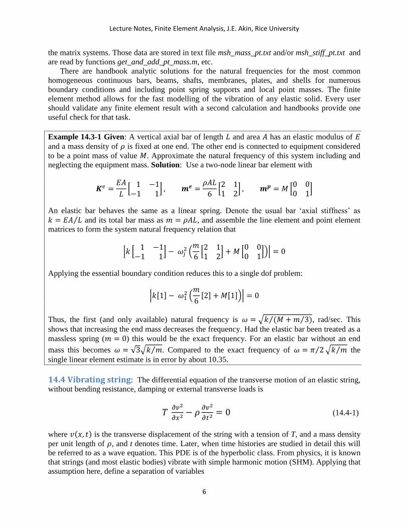
Example 14.3-1 Given: A vertical axial bar of length 𝐿 and area 𝐴 has an elastic modulus of 𝐸
and a mass density of 𝜌 is fixed at one end. The other end is connected to equipment considered
to be a point mass of value 𝑀. Approximate the natural frequency of this system including and
neglecting the equipment mass. Solution: Use a two-node linear bar element with
𝑲𝑒 =𝐸𝐴
𝐿[ 1 −1−1 1
] , 𝒎𝒆 =𝜌𝐴𝐿
6[2 11 2
] , 𝒎𝒑 = 𝑀 [0 00 1
]
An elastic bar behaves the same as a linear spring. Denote the usual bar ‘axial stiffness’ as
𝑘 = 𝐸𝐴 𝐿⁄ and its total bar mass as 𝑚 = 𝜌𝐴𝐿, and assemble the line element and point element
matrices to form the system natural frequency relation that
|𝑘 [ 1 −1−1 1
] − 𝜔𝑗2 (
𝑚
6[2 11 2
] + 𝑀 [0 00 1
])| = 0
Applying the essential boundary condition reduces this to a single dof problem:
|𝑘[1] − 𝜔12 (
𝑚
6[2] + 𝑀[1])| = 0
Thus, the first (and only available) natural frequency is 𝜔 = √𝑘 (𝑀 + 𝑚 3⁄ )⁄ , rad/sec. This
shows that increasing the end mass decreases the frequency. Had the elastic bar been treated as a
massless spring (𝑚 = 0) this would be the exact frequency. For an elastic bar without an end
mass this becomes 𝜔 = √3√𝑘 𝑚⁄ . Compared to the exact frequency of 𝜔 = 𝜋 2⁄ √𝑘 𝑚⁄ the
single linear element estimate is in error by about 10.35.
14.4 Vibrating string: The differential equation of the transverse motion of an elastic string,
without bending resistance, damping or external transverse loads is
𝑇 𝜕𝑣2
𝜕𝑥2− 𝜌
𝜕𝑣2
𝜕𝑡2= 0 (14.4-1)
where 𝑣(𝑥, 𝑡) is the transverse displacement of the string with a tension of T, and a mass density
per unit length of 𝜌, and t denotes time. Later, when time histories are studied in detail this will
be referred to as a wave equation. This PDE is of the hyperbolic class. From physics, it is known
that strings (and most elastic bodies) vibrate with simple harmonic motion (SHM). Applying that
assumption here, define a separation of variables

Lecture Notes, Finite Element Analysis, J.E. Akin, Rice University
7
𝑣(𝑥, 𝑡) = 𝑣𝑜(𝑥) sin(𝜔𝑡) (14.4-2)
where 𝑣𝑜(𝑥) is a “mode shape” defining the shape of the string along the x-direction as it
changes between positive and negative values that change with a frequency of ω. The second
time derivative of that assumption is
𝜕𝑣2
𝑑𝑡2= −𝜔2𝑣𝑜(𝑥) sin(𝜔𝑡) = −𝜔2 𝑣(𝑥, 𝑡)
The assumption of SHM changes the hyperbolic PDE over time and space into an elliptic ODE
in space:
𝑇 𝑑𝑣2
𝑑𝑥2+ 𝜌𝜔2𝑣 = 0 (14.4-3)
When the ODE has an unknown global constant (𝜔2) multiplying the solution value it is
called a scalar Helmholtz equation. This has the usual EBC and NBC options to define a unique
solution. For a guitar string, the usual EBCs are that both ends have zero transverse
displacements. Use of the Galerkin method and integration by parts (the introduction of the
NBCs) gives the governing integral form
𝐼 = [𝑣 (𝑇𝑑𝑣
𝑑𝑥 )]𝐿 0
− ∫𝑑𝑣
𝑑𝑥(𝑇
𝑑𝑣
𝑑𝑥)
𝐿
0𝑑𝑥 + ∫ 𝑣(𝑥) 𝐿
0𝜌 𝜔2 𝑣(𝑥) 𝑑𝑥 = 0 (14.4-4)
Next, introduce a finite element mesh and the usual element interpolations that in each element
𝑣(𝑥) = 𝑯(𝑟) 𝒗𝒆 = (𝑯(𝑟) 𝒗𝒆)𝑻 = 𝒗𝒆𝑻𝑯(𝑟)𝑻
Noting that the frequency, 𝜔, is an unknown global constant it is pulled outside the spatial
integral and will also be pulled outside the governing matrix system: [𝑺 − 𝜔2𝑴]{𝒗} = 𝒄𝑵𝑩𝑪.
When the EBCs of 𝑣(0) = 0 = 𝑣(𝐿) are enforced the rows in 𝒄𝑵𝑩𝑪 associated with the
remaining free DOFs are zero and the reduced problem is the same as (14.2-2).
The typical element stiffness and consistent mass matrices are
𝑲𝒆 = ∫𝑑𝑯(𝑟)
𝑑𝑥
𝑇
𝐿𝑒 𝑇𝑒 𝑑𝑯(𝑟)
𝑑𝑥 𝑑𝑥, 𝑴𝒆 = ∫ 𝑯(𝑟)𝑇
𝐿𝑒 𝜌𝑒𝑯(𝑟)𝑑𝑥 (14.4-5)
For constant properties and a constant Jacobian the closed form matrices for the two-node and
three-node Lagrangian line elements are
𝑲𝒆 =𝑇𝑒
𝐿𝑒[ 1 −1−1 1
] , 𝑴𝒆 = 𝜌𝑒𝐿𝑒
6[2 11 2
] (14.4-6)
𝑲𝒆 =𝑇𝑒
3𝐿𝑒 [ 7 −8 1−8 16 −8 1 −8 7
] , 𝑴𝒆 = 𝜌𝑒𝐿𝑒
30[ 4 2 −1 2 16 2−1 2 4
], (14.4-7)
respectively. The resulting vibration shapes (mode shapes) come in sets that are either symmetric
or anti-symmetric with respect to the center of the string.
Note that the assumptions imply that the string has slope continuity along its entire length
(with unknown values at the support points). That observation suggests that using Hermite
Lecture Notes, Finite Element Analysis, J.E. Akin, Rice University
8
elements will give more accurate eigenvalues and more physically realistic mode shape plots.
For the two-node cubic Hermite element the nodal unknowns are the string deflection and its
slope 𝒗𝒆𝑇 = [𝑣1 𝜃1 𝑣2 𝜃2], where 𝜃 denotes the slope of the string. From Chapter 8, and
the summary, the element matrices are
𝑲𝒆 =𝑇𝑒
30 𝐿𝑒[
36 3𝐿𝑒
3𝐿𝑒 4𝐿𝑒2−36 3𝐿𝑒
−3𝐿 −𝐿𝑒2
−36 −3𝐿𝑒
3𝐿𝑒 −𝐿𝑒2 36 −3𝐿𝑒
−3𝐿 4𝐿𝑒2
],
𝑴𝒆 =𝜌𝑒𝐿𝑒
420[
156 22𝐿𝑒
22𝐿𝑒 4𝐿𝑒254 −13𝐿𝑒
13𝐿𝑒 −3𝐿𝑒2
54 13𝐿𝑒
−13𝐿𝑒 −3𝐿𝑒2156 −22𝐿𝑒
−22𝐿𝑒 4𝐿𝑒2
]. (14.4-8)
The disadvantage of that approach is that the eigen-problem is twice as large as the one using
Lagrange interpolation and the same number of nodes. But it should give results more accurate
than a Lagrange element solution with twice as many nodes (without interior supports).
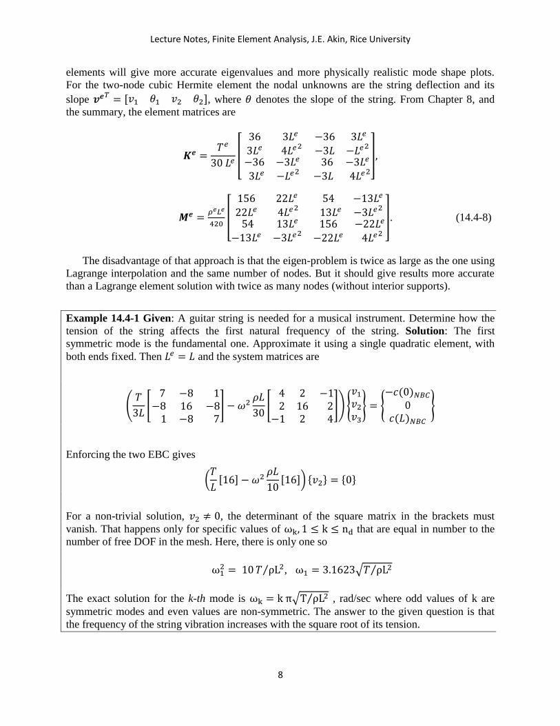
Example 14.4-1 Given: A guitar string is needed for a musical instrument. Determine how the
tension of the string affects the first natural frequency of the string. Solution: The first
symmetric mode is the fundamental one. Approximate it using a single quadratic element, with
both ends fixed. Then 𝐿𝑒 = 𝐿 and the system matrices are
(𝑇
3𝐿[ 7 −8 1−8 16 −8 1 −8 7
] − 𝜔2𝜌𝐿
30[ 4 2 −1 2 16 2−1 2 4
]) {
𝑣1
𝑣2
𝑣3
} = {−𝑐(0)𝑁𝐵𝐶
0𝑐(𝐿)𝑁𝐵𝐶
}
Enforcing the two EBC gives
(𝑇
𝐿[16] − 𝜔2
𝜌𝐿
10[16]) {𝑣2} = {0}
For a non-trivial solution, 𝑣2 ≠ 0, the determinant of the square matrix in the brackets must
vanish. That happens only for specific values of ωk, 1 ≤ k ≤ nd that are equal in number to the
number of free DOF in the mesh. Here, there is only one so
ω12 = 10𝑇 ρL2⁄ , ω1 = 3.1623√𝑇 ρL2⁄
The exact solution for the k-th mode is ωk = k π√T ρL2⁄ , rad/sec where odd values of k are
symmetric modes and even values are non-symmetric. The answer to the given question is that
the frequency of the string vibration increases with the square root of its tension.

Lecture Notes, Finite Element Analysis, J.E. Akin, Rice University
9
Here, the single quadratic element has only 0.66 % error in the first natural frequency. The
first mode shape is a half-sine curve, the amplitude of which is normalized to unity. The half-sine
mode shape is approximated spatially by a parabolic segment in a single element model.
Example 14.4-2 Given: Write a Matlab script to find the first three frequencies of the tensioned
string using a uniform mesh with two quadratic Lagrangian line elements where 𝑇 = 6𝑒5 𝑁,
𝐿 = 2 𝑚, and 𝜌 = 0.0234 𝑘𝑔/𝑚. Solution: Figure 14.4-1 details all of the required calculations
(but it does not list the computed mode shapes. The coordinates and properties are set manually
and (14.4-7) is inserted to build the element matrices once since they are the same for each
element. The loop over each element defines the element connection list manually and uses it to
assemble the two elements. The EBCs eliminate the first and fifth DOF, so only rows and
columns 2 through 4 of the two square matrices are passed to the Matlab function eig.m which
returns the mode shapes (as columns of a square matrix, and the square of the natural frequencies
(ωk2) as the diagonal elements of a second square matrix. Then the square root gives the three
actual frequencies, which are compared to the exact values. (The script String_vib_2_L3.m is
included in the Applications Library.) The execution of the script lists the mode shapes as
Mode 1 Mode 2 Mode 3
0.0000 0.0000 0.0000
0.7068 -1.0000 0.4068
1.0000 0.0000 -1.0000
0.7068 1.0000 0.4068
0.0000 0.0000 0.0000

Lecture Notes, Finite Element Analysis, J.E. Akin, Rice University
10
Figure 14.4-1 Tensioned string eigenvalue-eigenvector calculations

Lecture Notes, Finite Element Analysis, J.E. Akin, Rice University
11
Example 14.4-3 Given: Use a quadratic line element fixed at one end, with and averaged mass
matrix, to approximate the first two frequencies of axial vibration, and compare them to the exact
values of 𝜋 2⁄ and3𝜋 2⁄ times√𝐸𝐴 𝑚𝐿⁄ . Solution: The stiffness and averaged mass matrices are
given in the summary. The natural frequency problem is
(𝐸𝑒𝐴𝑒
3 𝐿𝑒[ 7 −8 1−8 16 −8 1 −8 7
] − 𝜆𝑗
𝑚𝑒
60[ 9 2 −1 2 36 2−1 2 9
])𝒖𝒋𝒆 = {
−𝑐(0)𝑁𝐵𝐶
00
}
Enforcing the EBC at node 1, reduces the problem to two degrees of freedom. The general eigen-
problem is
|𝐸𝑒𝐴𝑒
3 𝐿𝑒 [ 16 −8−8 7
] − 𝜆𝑗𝑚𝑒
60[36 22 9
]| = 0.
Setting the determinant to zero gives the characteristic equation
0 = [240 𝐸𝐴2 − 107𝐸𝐴 𝑚𝐿 𝜆 + 4𝐿2𝑚2 𝜆2 ] 45 𝐿2⁄
Calculating the two roots of the quadratic equation gives
𝜆1 = 𝜔12 = (107 − √7609) 𝐸𝐴 (8 𝑚 𝐿) → 𝜔1⁄ = 1.5720√𝐸𝐴 𝑚𝐿⁄ rad/sec
𝜆2 = 𝜔22 = (107 + √7609)𝐸𝐴 (8 𝑚 𝐿)⁄ → 𝜔2 = 4.9273√𝐸𝐴 𝑚𝐿⁄
This gives the first two frequency errors of 0.08% and 4.56%, respectively. Changing the
interpretation of the coefficients to torsional shafts, this corresponds to the free vibration of a
fixed-free shaft.
14.5 Torsional vibrations: The equation of motion of a vibrating torsional shaft or drill
string is of the same form as the transvers string vibration:
𝐺𝐽𝜕2𝜃
𝜕𝑥2 − 𝜌𝐽𝜕2𝜃
𝜕𝑡2 = 0 (14.5-1)
where 𝐺 is the material shear modulus, 𝐽 is the cross-section polar moment of inertia, 𝜌 is the
mass density per unit length, and 𝜃 is the (small) angle of twist of the shaft. The rotational inertia
of the shaft cross-section is defined as 𝐼 = 𝜌𝐽. By analogy to all of the stiffness matrices in
Section 14.4 the torsional stiffness matrix always includes the term 𝐺𝐽/𝐿 ≡ 𝑘𝑡 (divided by a
number). That term is known as the torsional stiffness of the shaft and many problems supply
that number to describe a shaft segment of length L.
It is common for equipment to be attached to a vibrating system. If the mass, or rotational
inertia, of the equipment is large then the usual practice is to treat the equipment as a point mass
and attach it to a node at an element interface. That is, the point mass (or inertia) is added to the
diagonal of the system mass matrix at the node where the equipment is located.
For a very long oil well drill string the end ‘bottom hole assembly’ (BHA) is relatively short
but has a very large rotational inertia. In the spring-mass simplified models this type of vibration
Lecture Notes, Finite Element Analysis, J.E. Akin, Rice University
12
is called the rotational pendulum. Thus, it is often treated as a point source of rotational inertia,
say 𝐼𝐿, that is placed on the diagonal of the rotational inertia matrix at the free end node.
That physical argument is justified by considering the nonessential boundary condition (from
14.4-4) at L:
[𝜃 (𝐺𝐽𝑑𝜃
𝑑𝑥 )]
𝐿≡ 𝜃𝐿 𝜏𝐿
where 𝜏𝐿is the external torque applied to the end of the shaft. The BHA is being considered as a
rotating planar rigid body. From Newton’s law the torque applied to a rotating rigid disk at its
center of mass is
𝜏𝑑𝑖𝑠𝑘 = 𝜌𝐽𝑑𝑖𝑠𝑘
𝜕2𝜃
𝜕𝑡2= 𝐼𝑑𝑖𝑠𝑘
𝜕2𝜃
𝜕𝑡2
But, for SHM at a frequency 𝜔 Newton’s law gives: 𝜏𝑑𝑖𝑠𝑘 = −𝜔2𝐼𝑑𝑖𝑠𝑘𝜃𝑑𝑖𝑠𝑘. An equal and
opposite torque is applied to the shaft from the disk, 𝜏𝐿 = −𝜏𝑑𝑖𝑠𝑘. Therefore, the system
analogous to (14.3-4) becomes
𝜃𝑑𝑖𝑠𝑘(𝜔2𝐼𝑑𝑖𝑠𝑘𝜃𝑑𝑖𝑠𝑘) − 0 − 𝜽𝑻𝑲𝜽 + 𝜔2𝜽𝑻𝑴𝜽 = 0
which shows that the planar disk inertia, 𝐼𝑑𝑖𝑠𝑘. is simply placed on the diagonal of the inertia matrix, 𝑴, at the (end) node where the disk is attached to the shaft, as expected.
Example 14.5-1 Given: Create a Matlab script to determine the natural frequencies of torsional
vibration of a circular vertical shaft, fixed at the top, and having a large point inertia at its end.
Solution: The script, Torsional_Vib_BHA_L3.m, is shown in Fig. 14.5-1 where it manually sets
data from a published study that has an exact analytic solution. It utilizes two three-node
quadratic line elements in a mesh with five nodes. Again, the Matlab eig function is used to solve
the eigen-problem equations.
Due to the top EBC, the system has four independent degrees of freedom and will thus give
frequency estimates for the first four modes that satisfy the EBC. Since the mesh is quite crude
only the first two modes are considered. The first frequency is overestimated by only 0.4% while
the second frequency is overestimated by 0.7%.
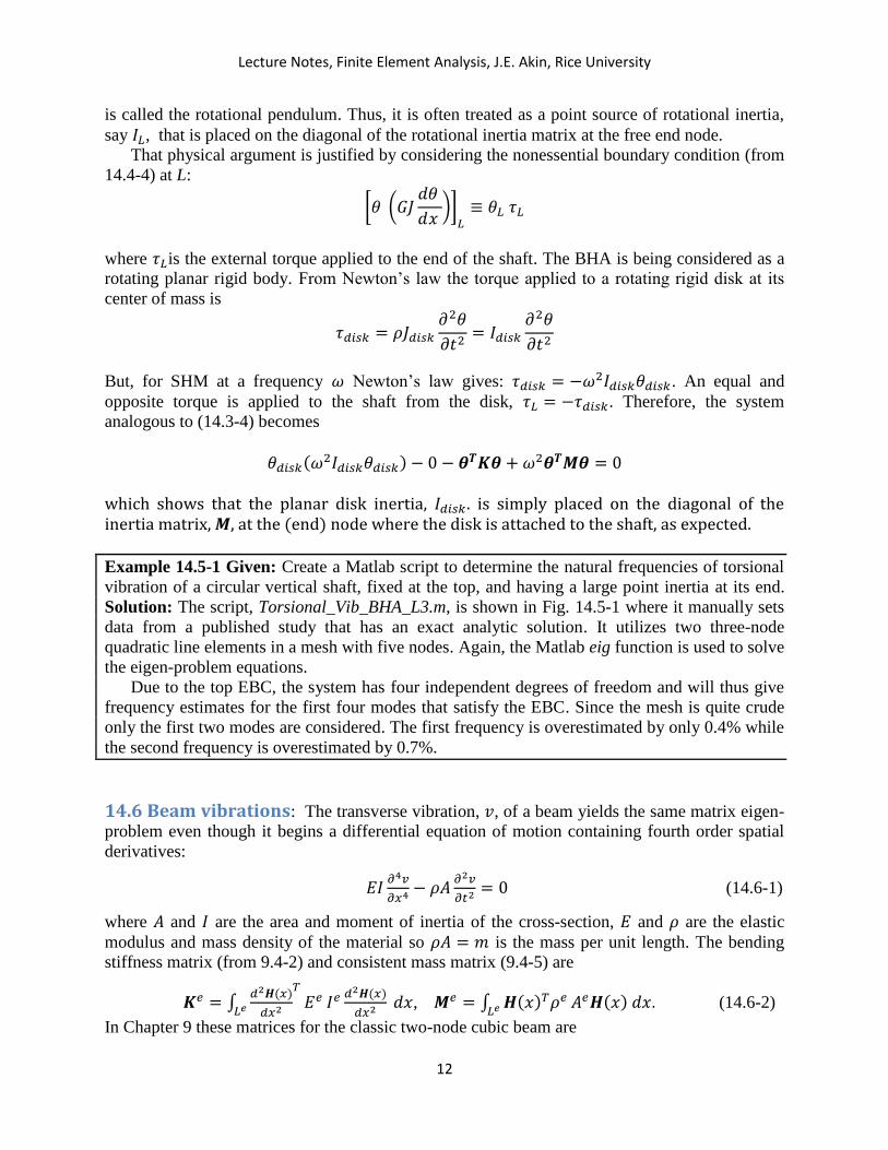
14.6 Beam vibrations: The transverse vibration, 𝑣, of a beam yields the same matrix eigen-
problem even though it begins a differential equation of motion containing fourth order spatial
derivatives:
𝐸𝐼𝜕4𝑣
𝜕𝑥4− 𝜌𝐴
𝜕2𝑣
𝜕𝑡2= 0 (14.6-1)
where 𝐴 and 𝐼 are the area and moment of inertia of the cross-section, 𝐸 and 𝜌 are the elastic
modulus and mass density of the material so 𝜌𝐴 = 𝑚 is the mass per unit length. The bending
stiffness matrix (from 9.4-2) and consistent mass matrix (9.4-5) are
𝑲𝑒 = ∫𝑑2𝑯(𝑥)
𝑑𝑥2
𝑇
𝐸𝑒
𝐿𝑒 𝐼𝑒 𝑑2𝑯(𝑥)
𝑑𝑥2 𝑑𝑥, 𝑴𝑒 = ∫ 𝑯(𝑥)𝑇𝜌𝑒
𝐿𝑒 𝐴𝑒𝑯(𝑥) 𝑑𝑥. (14.6-2)
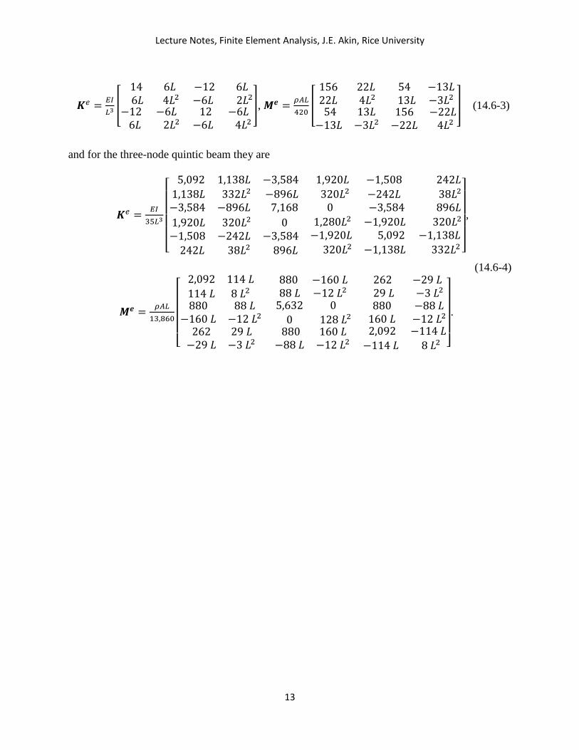
In Chapter 9 these matrices for the classic two-node cubic beam are
Lecture Notes, Finite Element Analysis, J.E. Akin, Rice University
13
𝑲𝑒 =𝐸𝐼
𝐿3 [
14 6𝐿 6𝐿 4𝐿2
−12 6𝐿−6𝐿 2𝐿2
−12 −6𝐿 6𝐿 2𝐿2
12 −6𝐿−6𝐿 4𝐿2
], 𝑴𝒆 =𝜌𝐴𝐿
420[
156 22𝐿 22𝐿 4𝐿2
54 −13𝐿 13𝐿 −3𝐿2
54 13𝐿−13𝐿 −3𝐿2
156 −22𝐿−22𝐿 4𝐿2
] (14.6-3)
and for the three-node quintic beam they are
𝑲𝑒 =𝐸𝐼
35𝐿3
[ 5,092 1,138𝐿 −3,584
1,138𝐿 332𝐿2 −896𝐿−3,584 −896𝐿 7,168
1,920𝐿 −1,508 242𝐿
320𝐿2 −242𝐿 38𝐿2
0 −3,584 896𝐿
1,920𝐿 320𝐿2 0−1,508 −242𝐿 −3,584
242𝐿 38𝐿2 896𝐿
1,280𝐿2 −1,920𝐿 320𝐿2
−1,920𝐿 5,092 −1,138𝐿
320𝐿2 −1,138𝐿 332𝐿2 ]
,
(14.6-4)
𝑴𝒆 =𝜌𝐴𝐿
13,860
[
2,092 114 𝐿
114 𝐿 8 𝐿2880 −160 𝐿 88 𝐿 −12 𝐿2
262 −29 𝐿 29 𝐿 −3 𝐿2
880 88 𝐿−160 𝐿 −12 𝐿2
5,632 0
0 128 𝐿2 880 −88 𝐿
160 𝐿 −12 𝐿2
262 29 𝐿−29 𝐿 −3 𝐿2
880 160 𝐿−88 𝐿 −12 𝐿2
2,092 −114 𝐿
−114 𝐿 8 𝐿2 ]
.

Lecture Notes, Finite Element Analysis, J.E. Akin, Rice University
14
Figure 14.5-1 Torsional frequencies for a shaft with end-point inertia
Lecture Notes, Finite Element Analysis, J.E. Akin, Rice University
15
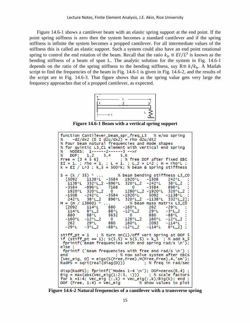
Figure 14.6-1 shows a cantilever beam with an elastic spring support at the end point. If the
point spring stiffness is zero then the system becomes a standard cantilever and if the spring
stiffness is infinite the system becomes a propped cantilever. For all intermediate values of the
stiffness this is called an elastic support. Such a system could also have an end point rotational
spring to control the end rotation of the beam. Recall that the ratio 𝑘𝑏 ≡ 𝐸𝐼 𝐿3⁄ is known as the
bending stiffness of a beam of span L. The analytic solution for the system in Fig. 14.6-1
depends on the ratio of the spring stiffness to the bending stiffness, say R≡ 𝑘/𝑘𝑏. A Matlab
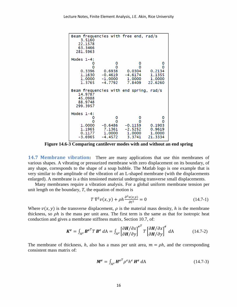
script to find the frequencies of the beam in Fig. 14.6-1 is given in Fig. 14.6-2, and the results of
the script are in Fig. 14.6-3. That figure shows that as the spring value gets very large the
frequency approaches that of a propped cantilever, as expected.
Figure 14.6-1 Beam with a vertical spring support
Figure 14.6-2 Natural frequencies of a cantilever with a transverse spring
Lecture Notes, Finite Element Analysis, J.E. Akin, Rice University
16
Figure 14.6-3 Comparing cantilever modes with and without an end spring
14.7 Membrane vibration: There are many applications that use thin membranes of
various shapes. A vibrating or pressurized membrane with zero displacement on its boundary, of
any shape, corresponds to the shape of a soap bubble. The Matlab logo is one example that is
very similar to the amplitude of the vibration of an L-shaped membrane (with the displacements
enlarged). A membrane is a thin tensioned material undergoing transverse small displacements.
Many membranes require a vibration analysis. For a global uniform membrane tension per
unit length on the boundary, T, the equation of motion is
𝑇 ∇2𝑣(𝑥, 𝑦) + 𝜌ℎ𝜕2𝑣(𝑥,𝑦)
𝜕𝑡2 = 0 (14.7-1)
Where 𝑣(𝑥, 𝑦) is the transverse displacement, 𝜌 is the material mass density, ℎ is the membrane
thickness, so 𝜌ℎ is the mass per unit area. The first term is the same as that for isotropic heat
conduction and gives a membrane stiffness matrix, Section 10.7, of:
𝑲𝒆 = ∫ 𝑩𝒆𝑇𝑇
A𝑒 𝑩𝒆 𝑑A = ∫ [𝜕𝑯 𝜕𝑥⁄
𝜕𝑯 𝜕𝑦⁄]𝒆𝑇
𝑇
A𝑒 [𝜕𝑯 𝜕𝑥⁄
𝜕𝑯 𝜕𝑦⁄]𝒆
𝑑A (14.7-2)
The membrane of thickness, ℎ, also has a mass per unit area, 𝑚 = 𝜌ℎ, and the corresponding
consistent mass matrix of:
𝑴𝒆 = ∫ 𝑯𝒆𝑇𝜌𝑒ℎ𝑒
A𝑒 𝑯𝒆 𝑑A (14.7-3)

Lecture Notes, Finite Element Analysis, J.E. Akin, Rice University
17
which assemble into the vibration eigen-problem [𝑲 − 𝜔2𝑗 𝑴]𝜹𝒋 = 0. The form of those
element matrices were developed in Chapter 10.
The vibration of a flat L-shaped membrane to date has no analytic solution and requires a
numerical solution. Very accurate theoretical upper and lower bounds for the natural frequencies
of the first ten modes have been published. Consider an L-shaped membrane made up of three
unit square sub-regions. That membrane is very similar to the one that serves as the Matlab logo.
Note that any L-shaped membrane has a singular point at the re-entrant corner. For static
solutions, the radial gradient of the deflected shape at that corner is theoretically infinite and no
finite element solution with a uniform mesh will ever reach the theoretical solution. Not only
does the asymptotic analytic solution have an infinite gradient, but that gradient changes rapidly
with the angle from the first exterior edge to the second edge. These two facts mean that ideally
the mesh should be manually controlled to make the elements smaller as they radially approach
any singular point, but the mesh should have several elements sharing one vertex at the singular
point.
In the early days of finite element solutions, when the available memory was very very small,
a special type of ‘singularity elements’ were developed to include in the mesh at singular points.
Today, with adaptive mesh generation it is up to the user to create a reasonable mesh refinement
at any re-entrant corner. (For adaptive error analysis solutions the user must also limit the size of
the smallest element at a re-entrant corner to prevent all new elements being placed there in the
attempt to calculate an infinite gradient.)
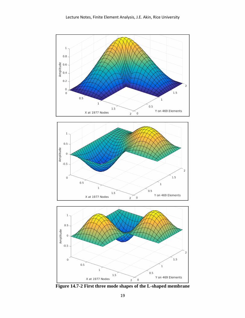
For a regular shape, like an L-shaped membrane, symmetric and anti-symmetric modes may
negate the presence of a re-entrant corner. For example, it will be seen that the third mode of the
L-shaped membrane has the same mode shape (with +, -, + signs) in each of the three square
sub-regions. Thus, the interior vertical and horizontal lines passing through the corner have zero
displacement amplitudes. In other words, it is exactly like computing the first mode of a square
with no re-entrant corner.
Figure 14.7-1 shows a mesh of nine-noded quadrilaterals and 1,977 degrees of freedom
(nodes) that were used to mode the L-shaped membrane and the anti-symmetric modes of a U-
shaped membrane (where the bottom line of Fig. 14.7-1 has a natural boundary condition of zero
normal slope). The bottom portion shows the mode 1 shape obtained with four-node quadrilateral
elements and 252 DOF. The two first mode frequency estimates, 68.18 Hz and Y, differ by less
than 4%. That view angle, like the one of the Matlab logo, hides the reentrant corner.
The calculations were done by the script Membrane_vibration.m which is in the Application
Library. It accepts a membrane of any shape meshed with any element in the provided library.
The elements are numerically integrated to alloy for curved membranes and variable Jacobian
elements. To produce the mode shape plots invokes the script mode_shape_surface.m which is in
the general function library.

Lecture Notes, Finite Element Analysis, J.E. Akin, Rice University
18
.
Figure 14.7-1 L-shaped membrane first mode of vibration with Q9 and Q4 elements
Lecture Notes, Finite Element Analysis, J.E. Akin, Rice University
19
Figure 14.7-2 First three mode shapes of the L-shaped membrane

Lecture Notes, Finite Element Analysis, J.E. Akin, Rice University
20
Figure 14.7-3 First three symmetric modes of U-shaped membrane
Lecture Notes, Finite Element Analysis, J.E. Akin, Rice University
21
14.8 Structural buckling: There are two major categories leading to the sudden failure of a
mechanical component: structural instability, which is often called buckling, and brittle material
failure. Buckling failure is primarily characterized by a sudden, and usually catastrophic, loss of
structural stiffness that usually renders the structure unusable. The buckling estimate is
computed from a finite element eigen-problem solution. Slender or thin-walled components
under compressive stress are susceptible to buckling. Buckling studies are much more sensitive
to the component restraints that a normal stress analysis. A buckling mode describes the
deformed shape the structure assumes (but not the direction) when it buckles, but (like a
vibration mode) says nothing about the numerical values of the displacements or stresses. The
numerical values may be displayed, but are only relative and are usually scaled to have a
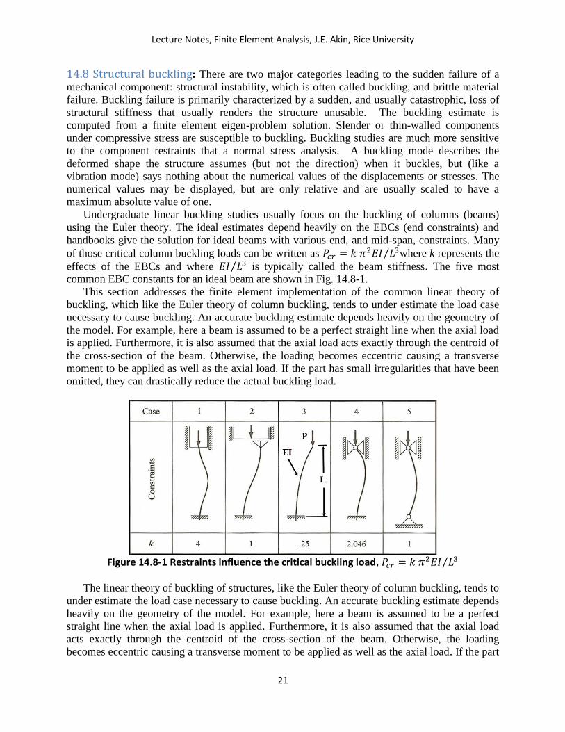
maximum absolute value of one. Undergraduate linear buckling studies usually focus on the buckling of columns (beams)
using the Euler theory. The ideal estimates depend heavily on the EBCs (end constraints) and
handbooks give the solution for ideal beams with various end, and mid-span, constraints. Many
of those critical column buckling loads can be written as 𝑃𝑐𝑟 = 𝑘 𝜋2𝐸𝐼 𝐿3⁄ where k represents the
effects of the EBCs and where 𝐸𝐼 𝐿3⁄ is typically called the beam stiffness. The five most
common EBC constants for an ideal beam are shown in Fig. 14.8-1.
This section addresses the finite element implementation of the common linear theory of
buckling, which like the Euler theory of column buckling, tends to under estimate the load case
necessary to cause buckling. An accurate buckling estimate depends heavily on the geometry of
the model. For example, here a beam is assumed to be a perfect straight line when the axial load
is applied. Furthermore, it is also assumed that the axial load acts exactly through the centroid of
the cross-section of the beam. Otherwise, the loading becomes eccentric causing a transverse
moment to be applied as well as the axial load. If the part has small irregularities that have been
omitted, they can drastically reduce the actual buckling load.
Figure 14.8-1 Restraints influence the critical buckling load, 𝑃𝑐𝑟 = 𝑘 𝜋2𝐸𝐼 𝐿3⁄
The linear theory of buckling of structures, like the Euler theory of column buckling, tends to
under estimate the load case necessary to cause buckling. An accurate buckling estimate depends
heavily on the geometry of the model. For example, here a beam is assumed to be a perfect
straight line when the axial load is applied. Furthermore, it is also assumed that the axial load
acts exactly through the centroid of the cross-section of the beam. Otherwise, the loading
becomes eccentric causing a transverse moment to be applied as well as the axial load. If the part
Lecture Notes, Finite Element Analysis, J.E. Akin, Rice University
22
has small irregularities that have been omitted, they can drastically reduce the actual buckling
load.
When a constant axial load acts along the entire beam, say 𝑁𝐵, it factors out of the element
initial stress (geometric stiffness) matrices and the assembly process to appear as a constant in
the system matrices. The goal is to find the scaling up or down of the applied load that causes
linear buckling. That scale factor is called the “buckling load factor (BLF)” and replacing 𝑁𝐵with
𝐵𝐿𝐹 × 𝑁𝐵 leads to a buckling eigen-problem to determine the value of BLF.
For a general structure with a set of loads (called a load case) the system geometric stiffness
matrix depends on the stress in each element. That means that it depends on all of the assembled
loads, say 𝐹𝑟𝑒𝑓. In general, a linear static analysis is completed and the deflections are
determined from the system equilibrium using the elastic stiffness matrix and any foundation
stiffness matrix: [𝑲𝑬 + 𝑲𝒌
]{𝒗 } = {𝑭𝒓𝒆𝒇 }. Those displacements are post-processed to determine
the stresses in each element. Then each element geometric stiffness matrix is calculated from
those stresses. The element stresses, and thus its geometric stiffness matrix, is directly proportion
to the resultant system load, so as the loads are scaled by the buckling factor the system
geometric stiffness matrix increases by the same amount
𝑭 → 𝐵𝐿𝐹 𝑭𝒓𝒆𝒇 , 𝑲𝑵
→ 𝐵𝐿𝐹 𝑲𝒓𝒆𝒇
The scaling value, BLF, that renders the combined system stiffness to have a zero
determinant (that is to become unstable) is the increase (or decrease) of all of the applied loads
that will cause the structure to buckle. That critical value is calculated from a buckling eigen-
problem using the previous matrices plus the geometric stiffness matrix based on the current load
case:
|𝑲𝑬 + 𝑲𝒌
− 𝐵𝐿𝐹 𝑲𝒓𝒆𝒇 | = 0 (14.8-1)
That equation is solved for the value of the BLF. Then the system load case that would
theoretically cause buckling is 𝐵𝐿𝐹 𝑭𝒓𝒆𝒇 . The solution of the eigen-problem also yields the
relative buckled mode shape (eigen-vector), 𝒗𝑩𝑭. The magnitude of the buckling mode shape
displacements are arbitrary and most commercial software normalizes them to range from 0 to 1.
For straight beams with an axial load several of the above steps are skipped because each
element’s axial stress and its geometric stiffness matrix are known by inspection. The eigenvalue
BLF is the ratio of the buckling load case to the applied load case. The following table gives the
interpretation of possible values for the buckling factor.
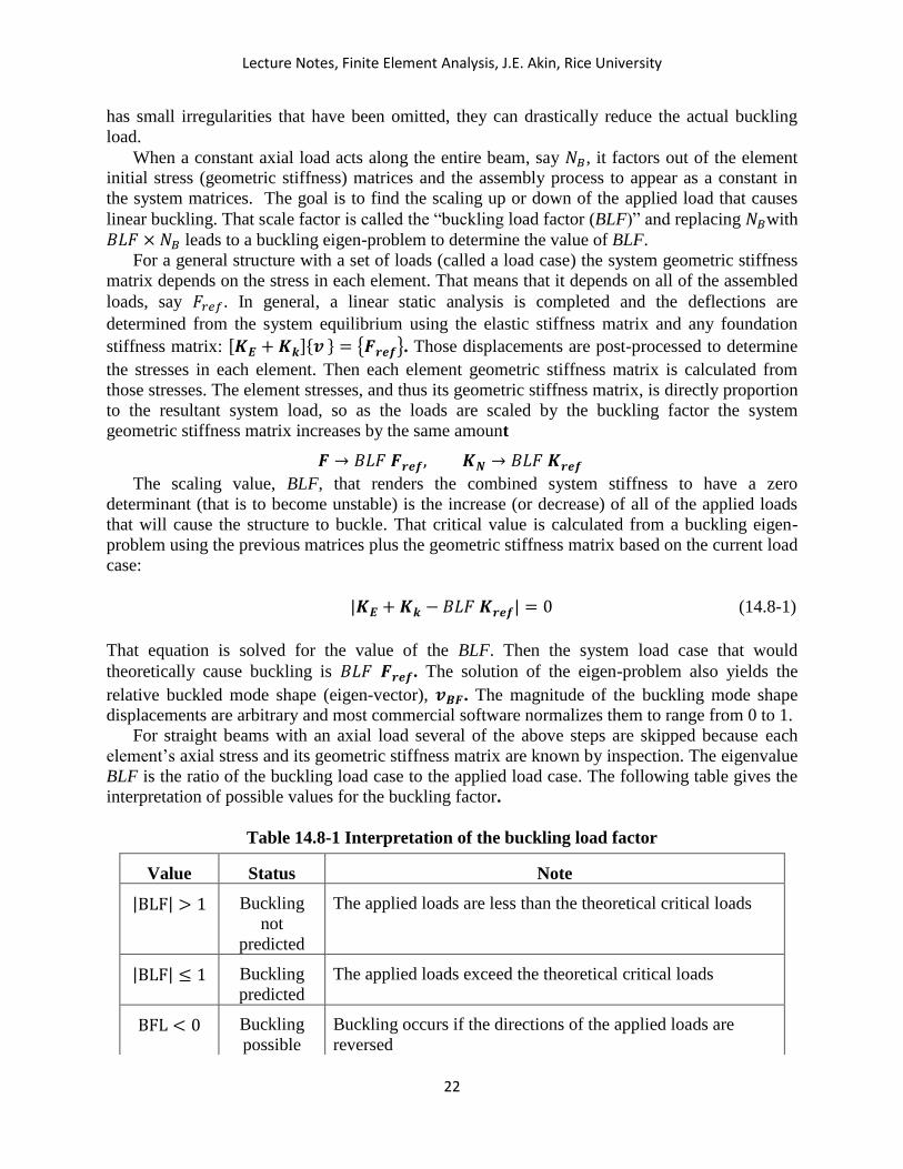
Table 14.8-1 Interpretation of the buckling load factor
Value Status Note
|BLF| > 1 Buckling
not
predicted
The applied loads are less than the theoretical critical loads
|BLF| ≤ 1 Buckling
predicted
The applied loads exceed the theoretical critical loads
BFL < 0 Buckling
possible
Buckling occurs if the directions of the applied loads are
reversed

Lecture Notes, Finite Element Analysis, J.E. Akin, Rice University
23
In theory, there are as many buckling modes as there are DOF in a structure. Due to the
limitations of linear buckling theory, only the first buckling mode is of practical importance.
Structural buckling is usually instantaneous and catastrophic. A Factor of Safety of four is often
applied to linear buckling estimates. There are commercial finite element systems that can solve
the more accurate nonlinear post-buckling behavior of structures.
The estimated buckling force can be unrealistically large. A linear buckling calculation
implies that the compression load-deflection relation, and thus the material compression stress-
strain relation is linear. That is true only up to where the stress reaches the material compressive
yield stress, say 𝑆𝑦𝑐. In other words, the critical compressive stress, 𝜎𝑐𝑟 = 𝑃𝑐𝑟 𝐴⁄ , caused by the
critical force, 𝑃𝑐𝑟, must also be considered. To do that the critical for relation must be re-written
in terms of the cross-sectional area. That is done by using the geometric ‘radius of gyration’, 𝑟𝑔,
defined as 𝐼 ≡ 𝐴 𝑟𝑔2. Then for typical boundary conditions
𝑃𝑐𝑟 = 𝑘𝜋2 𝐸𝐼 𝐿2⁄ = 𝑘𝜋2𝐸(𝐴 𝑟𝑔2) 𝐿2⁄ = 𝑘𝜋2𝐸𝐴 (𝐿 𝑟𝑔⁄ )
2⁄
where the ratio 𝐿 𝑟𝑔⁄ is known as the ‘slenderness ratio’ of the cross-section. It is evaluated at the
location of the smallest 𝐼 found on any plane perpendicular to the axis of the load. The critical
compressive stress is 𝜎𝑐𝑟 = 𝑃𝑐𝑟 𝐴⁄ = 𝑘𝜋2𝐸 (𝐿 𝑟𝑔⁄ )2
⁄ ≤ 𝑆𝑦𝑐. This gives the theoretical relation
𝜎𝑐𝑟 = 𝑃𝑐𝑟 𝐴 ≤⁄ 𝑆𝑦𝑐(𝐿 𝑟𝑔⁄ )2
𝑘𝜋2𝐸⁄ .
| P
v
/| 1
Slope 1:1 / | L constant EA
pin 3 / | 2 pin
Figure 14.8-2 Simple truss with a potential buckling load
Example 14.8-1 Given: The constant EA truss in Fig. 14.8-2 has the connection list [1 2, 3 1]
and a previous analysis showed that the inclined member is force (and stress) free and the
vertical (first) carries an axial force of N = -P. Repeat the truss analysis with the addition of the
initial stress (geometric) stiffnesses to determine the value of P required to cause the truss to
buckle (in its original plane). Solution: The elastic stiffness matrix of a truss member must be
rotated from its horizontal position. The direction angles of the first (vertical) and second
(inclined) members are 𝐶𝑥 = 90°, 𝐶𝑦 = 0, and 𝐶𝑥 = 45°, 𝐶𝑦 = 45°, respectively. Thus, their
respective transformation sub-matrices are
𝒕𝑒=1(𝜃) = [ 0 1−1 0
0 00 0
] , 𝒕𝑒=2(𝜃) =1
√2[ 1 1−1 1
0 00 0
] , [𝑻(𝜃)] = [𝒕(𝜃) 𝟎𝟎 𝒕(𝜃)
]

Lecture Notes, Finite Element Analysis, J.E. Akin, Rice University
24
and the original and transformed elastic stiffness matrices, 𝑺𝑮𝒆 = [𝑻(𝜃)]𝑻𝑺𝑳
𝒆 [𝑻(𝜃)], are
DOF 1 2 3 4 5 6 1 2
𝑺𝑬𝒆 =
𝐸𝑒𝐴𝑒
𝐿𝑒 [ 1 0 0 0
−1 0 0 0
−1 0 0 0
1 0 0 0
] , 𝑺𝑬𝒆=𝟏 =
𝐸 𝐴
𝐿 [ 0 00 1
0 00 −1
0 0 0 −1
0 00 1
] , 𝑺𝑬𝒆=𝟐 =
𝐸 𝐴
(√2𝐿)
1
2[ 1 1 1 1
−1 −1−1 −1
−1 −1−1 −1
1 1 1 1
]
The initial stress (geometric) stiffness matrix transforms in the same manner:
DOF 1 2 3 4
𝑺𝒊𝒆 =
𝑁
𝐿 [ 0 00 1
0 00 −1
0 0 0 −1
0 00 1
] , 𝑺𝒊𝒆=𝟏 =
−𝑃
𝐿 [ 1 0 0 0
−1 0 0 0
−1 0 0 0
1 0 0 0
] , 𝑺𝒊𝒆=𝟐 = 𝟎.
The structure has six degrees of freedom, but only the first two are free, so only those partitions
need to be assembled:
[(𝐸 𝐴
𝐿 [0 00 1
] +𝐸 𝐴
2√2 𝐿 [1 11 1
]) − 𝑃 (1
𝐿[1 00 0
])] {𝑢𝟏
𝑢𝟐} = {
00}
The critical buckling force causes the determinant to vanish:
|(
𝐸𝐴
2√2 𝐿 −𝑃𝑐𝑟𝑖𝑡
𝐿)
𝐸𝐴
2√2 𝐿
𝐸𝐴
2√2 𝐿 (1 + 2√2)𝐸𝐴
2√2 𝐿
| = 0 =𝐸𝐴
2√2 𝐿 |[
(1 − 2√2 𝑃𝑐𝑟𝑖𝑡 𝐸𝐴⁄ ) 1
1 (1 + 2√2)]|.
Evaluating the determinant gives the critical load of 𝑃𝑐𝑟𝑖𝑡 = 𝐸𝐴 (2√2 − 1) 7⁄ = 0.261 𝐸𝐴,
which is the same value obtained from the mechanics of materials.
Example 14.8-2 Given: A fixed–pinned beam (case 4 of Fig. 14.8-1) has an axial compression
load of P. Determine the approximate value of P that causes the beam to buckle. Solution: A
single cubic beam has only one DOF, but could give an upper bound on the buckling load (try it).
A three degree of freedom model will give a better estimate. That can be a three-node mesh with
either two cubic beam elements or a single quintic element. They would both have the middle
and end slope as DOF, along with the middle transverse deflection to define the mode shape.
The elastic stiffness, geometric stiffness and mass matrices for the quintic beam (L3_C1)
were given in (9.5-2). For a single quintic element model the two stiffnesses matrices are

Lecture Notes, Finite Element Analysis, J.E. Akin, Rice University
25
𝑲𝑬 =𝐸𝐼
35 𝐿3
[ 5,092 1,138 𝐿 −3,584
1,138 𝐿 332 𝐿2 −896 𝐿−3,584 −896 𝐿 7,168
1,920 𝐿 −1,508 242 𝐿
320 𝐿2 −242 𝐿 38 𝐿2
0 −3,584 896 𝐿
1,920 𝐿 320 𝐿2 0−1,508 −242 𝐿 −3,584
242 𝐿 38 𝐿2 896 𝐿
1,280 𝐿2 −1,920 𝐿 320 𝐿2
−1,920 𝐿 5,092 −1,138 𝐿
320 𝐿2 −1,138 𝐿 332𝐿 2 ]
𝑲𝑵 =−𝑃
630 𝐿
[ 1,668 39 𝐿
39 𝐿 28 𝐿2
−1,536 240 𝐿
−48 𝐿 −8 𝐿2−132 −9 𝐿 9𝐿 −5 𝐿2
−1,536 −48 𝐿
240 𝐿 −8 𝐿2
3,072 0
0 256 𝐿2−1,536 48 𝐿
−240 𝐿 −8 𝐿2
−132 9𝐿−9 𝐿 −5 𝐿2
−1,536 −240 𝐿
48 𝐿 −8 𝐿2
1,668 −39 𝐿
−39 𝐿 28 𝐿2]
,
corresponding to the DOF 𝒗𝑻 = [𝑣1 𝜃1 𝑣2 𝜃2 𝑣3 𝜃3] = [0 0 𝑣2 𝜃2 0 𝜃3], so
that only DOF 3, 4, and 6 are free. Substituting those three rows and columns into the eigen-
problem and multiplying by the coefficient of 𝑲𝑬 gives
|[7,168 0 896 𝐿
0 1,280 𝐿2 320 𝐿2
896 𝐿 320 𝐿2 332 𝐿2
] −𝑃
630 𝐿
35 𝐿3
𝐸𝐼[ 3,072 0 48 𝐿
0 256 𝐿2 −8 𝐿2
48 𝐿 −8 𝐿2 28 𝐿2
]| = 0 .
Defining the eigenvalue as 𝜆 ≡ 𝑃𝑐𝑟𝐿2 18 𝐸𝐼⁄ , setting the determinant to zero yields a cubic
characteristic equation −8 1 𝜆3 + 1575 𝜆2 − 6020 𝜆 + 4900 = 0.
Computing the roots of that polynomial gives: 𝜆3 = 14.6546, 𝜆2 = 3.6628, and 𝜆1 = 1.1270.
The smallest eigenvalue corresponds to the first, and most critical, buckling load. Therefore, the
estimated buckling load is 𝑃1 = 18 × 𝜆1 𝐸𝐼 𝐿2⁄ = 20.286 𝐸𝐼 𝐿2⁄ , where 𝐸𝐼 𝐿2⁄ is known as the
beam stiffness. The exact coefficient is 20.187. The quintic beam-column element gave an error
of 0.5%. Repeating this calculation with two cubic beam elements gives a 2.5% error.
Figure 14.8-3 Beam-column with axial load and vertical spring
Example 14.8-3 Given: Describe how the Ex. 14.8-2 changes if a transverse spring is present as
in Fig. 14.8-2. Solution: Only the active elastic stiffness matrix changes by adding the spring
stiffness to the diagonal location in 𝑲𝑬 corresponding to the node to which the spring is attached:
𝑲𝑬 =𝐸𝐼
35 𝐿3 [7,168 0 896 𝐿
0 1,280 𝐿2 320 𝐿2
896 𝐿 320 𝐿2 332 𝐿2
] + [𝑘 0 00 0 00 0 0
]

Lecture Notes, Finite Element Analysis, J.E. Akin, Rice University
26
which makes the first coefficient in the left matrix, after defining 𝜆, depend on the ratio of the
spring axial stiffness to the transverse beam stiffness, 𝐸𝐼 𝐿3⁄ :
(7,168 + 35 𝑘 𝐿3 𝐸𝐼⁄ ) = (7,168 + 35 𝑘 𝑘𝑏𝑒𝑎𝑚⁄ )
Increasing the sprint stiffness will slightly increase the critical buckling force. The spring makes
the algebra get much worse, but has no noticeable effect on how the numerical calculations are
done after the spring stiffness is scattered to the proper diagonal location.
Note that the limit of 𝑘 → ∞ makes the spring act as a second pin support at the mid-span.
That also cuts the free span length in half, significantly increases the bending stiffness, and then
the spring significantly increases the force required to buckle the column.
Example 14.8-3 Given: Write a Matlab script to implement the calculations given in Ex. 14.8-
1, and to plot the buckled mode shape. Solution: Such a script is in Fig. 14.8-3. The mechanics
calculations take about a dozen lines. After the EBCs are enforced only the mid-span
displacement, mid-span rotation, and the end-point rotation remain free (DOFs 3, 4, 6). Those
three rows and columns from the elastic stiffness and the geometric matrices are passed as input
arguments to the Matlab function eig which returns three critical BLF values and their
corresponding buckled mode shapes. The three BLF are extracted from the returned square
matrix into a vector using the Matlab function diag. That was done because eig does NOT
always return the eigenvalues in increasing order. The Matlab abs min function combination was
used to find which eigenvalue was the smallest and to grab that value. The location of the
smallest eigenvalue was then used to extract the column from the eigenvector square matrix
which corresponds to the lowest buckling mode shape. (Note, the higher buckling modes are not
important so an algorithm that finds and returns only the lowest eigenvalue is the most efficient
way to do buckling studies.) The lowest BLF is printed, along with that value reduced by a
Factor of Safety (FOS) of four. Then the retained buckling mode is plotted and saved.
The larger lower section of the figure primarily addresses the scaled magnitude of the fifth-
degree polynomial used to calculate the critical load. To list or graph the mode shape the full
system displacement vector must be restored by inserting the three free buckled displacement
components in with the prior three EBC values. The magnitudes of the components of the
buckling mode displacement are only relative, so they are scaled to have a maximum non-
dimensional value of one. Then the six element degrees of freedom are interpolated at many
points along the fifth degree polynomial to display the exact curve of the approximate buckled
mode shape. The location of the three element nodes, and a dashed line representing the original
column centerline are optionally added to provide a more informative graph (see Fig. 14.8-4).

Lecture Notes, Finite Element Analysis, J.E. Akin, Rice University
27
Figure 14.8-3 Linear buckling load and mode shape for a fixed-pinned beam

Lecture Notes, Finite Element Analysis, J.E. Akin, Rice University
28
Figure 14.8-4 Linear buckled mode shape estimate of fixed-pinned column
14.9 Beam frequency with an axial load: To determine the natural frequencies of a
structure subjected to an axial load the eigen-problem is |(𝑲𝑬 + 𝑲𝑵
) − 𝜔2𝑴| = 0, where 𝑲𝑬 is
the usual elastic stiffness matrix, 𝑲𝑵 is the geometric stiffness matrix associated with the axial
load, N, and 𝑴 is the usual mass matrix. When the axial load is an constant, say 𝑁𝐵, then it
factors out of each element geometric stiffness matrix and becomes a global constant after
assembly:
|(𝑲𝑬 + 𝑁𝐵𝑲𝒏
) − 𝜔2𝑴| = 0 (14.9-1)
where the unit initial stress matrix, Kn , is formed with a unit positive load. This equation shows
that any axial load, NB, has an influence on the natural frequency, ω. In general, a tensile force
(+) increases the natural frequency while a compression force (-) lowers the natural frequency.
One of the most common applications of this state is finding the natural frequencies of
turbine blades in jet engines. Their high rotational speed imposes a tension centripetal force on
the blades that increases with radial position. A static solution at a fixed rotational speed defines
the element stresses that in turn define the element geometric (initial stress) matrix. Then the
eigen-problem is solved to compute the blade frequencies at each rotational speed of the engine.
This eigen-problem is easily solved numerically. There are several published analytic
solutions for a beam-column with various essential boundary conditions. Still, a single finite
element can give an important insight into how the primary variables impact the resulting natural
frequency. Consider finding the natural frequency of a fixed-pinned column (case 4) subjected to
an axial tension force, P. A single cubic beam element model has only the single end rotation, 𝜃2,
as its one free degree of freedom. Substituting that term from the cubic beam matrices, from
(9.5-1), and (9.5-3), into the third row of the system matrix (14.9-1) gives:

Lecture Notes, Finite Element Analysis, J.E. Akin, Rice University
29
|𝐸𝐼
𝐿3[4𝐿2] +
𝑃
𝐿[2 𝐿2
15] − 𝜔2𝜌𝐴𝐿 [
4 𝐿2
420]| = 0
and dividing all terms by 𝐸𝐼 𝐿⁄ gives
4 + 𝑃𝐿2
𝐸𝐼
2
15− 𝜔2
𝜌𝐴𝐿4
𝐸𝐼= 0
so, the natural frequency squared is :
𝜔2 = 420𝐸𝐼
𝜌𝐴𝐿4{1 +
1
30
𝑃𝐿2
𝐸𝐼} = 420
𝐸𝐼
𝑚 𝐿3{1 +
1
30
𝑃
𝐿
𝐿3
𝐸𝐼}
where 𝑚 = 𝜌𝐴𝐿 is the mass of the beam, 𝐸𝐼 𝐿3⁄ is the beam elastic stiffness, and 𝑃 𝐿⁄ is the
beam geometric stiffness. The final frequency becomes
𝜔 = 20.49√𝐸𝐼
𝑚 𝐿3√1 +
1
30
𝑃
𝐿
𝐿3
𝐸𝐼, or 𝜔 ≡ 𝑛1√
𝐸𝐼
𝑚 𝐿3√1 +
1
𝑛2
𝑃
𝐿
𝐿3
𝐸𝐼 (14.9-2)
The last re-arranged term is the general form that the exact analytic solution takes for various
essential boundary conditions (that generate their corresponding 𝑛1 and 𝑛2 values). For
example, a pinned-pinned single span beam the i-th frequency has 𝑛1 = 𝜋 𝑖2 2⁄ , 𝑛2 = 𝜋2𝑖2. That
general form shows that when the axial load is tension (𝑃 > 0) the natural frequency is
increased. Conversely, when the load is compressive (𝑃 < 0) the natural frequency is reduced.
The lower limit is when the frequency goes to zero, which corresponds to the column buckling
(losing its stiffness): 𝑃𝑐𝑟 = −𝑛2𝐸𝐼 𝐿2⁄ . The theoretical relation between the square of the
frequency and the axial load is linear and is shown for compression loads in Fig. 14.9-1.
If the above single cubic element is changed to a pinned-pinned pair of EBCs, then it has
two dof and thus two natural frequencies. Their values are
𝜔1 = 10.954√𝐸𝐼
𝑚 𝐿3√1 +
1
12
𝑃
𝐿
𝐿3
𝐸𝐼 , 𝜔2 = 50.200√
𝐸𝐼
𝑚 𝐿3√1 +
1
60
𝑃
𝐿
𝐿3
𝐸𝐼
and setting 𝜔1 = 0 gives a buckling load estimate of 𝑃1 = −12 𝐸𝐼 𝐿2⁄ which is about 27%
higher than the exact value of −𝜋2 𝐸𝐼 𝐿2⁄ .

Lecture Notes, Finite Element Analysis, J.E. Akin, Rice University
30
Figure 14.9-1 Square of column frequency is proportional to axial load
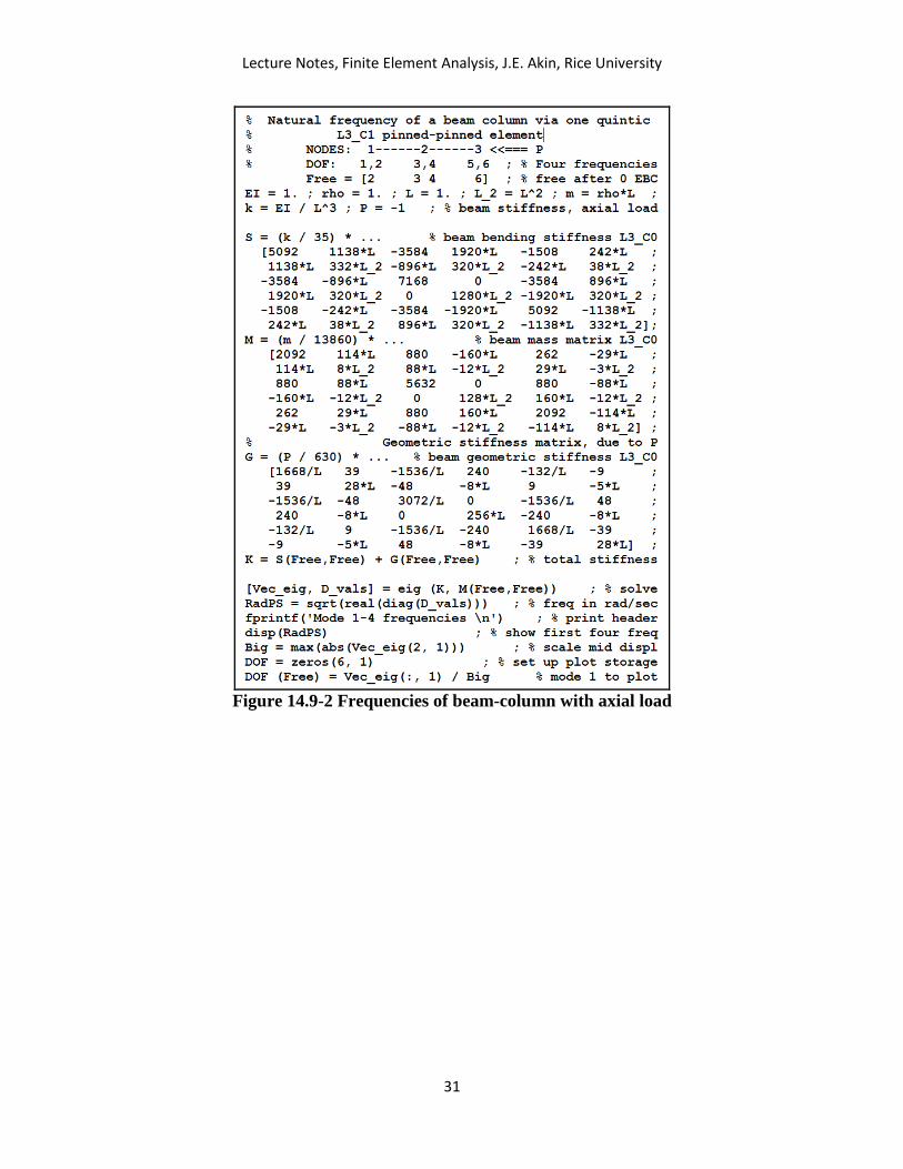
Example 14.9-1 Given: Write a Matlab script to determine the natural frequencies of the quintic
fixed–pinned beam-column (case 4 of Fig. 14.8-1) in Example 14.8-1 with an axial tension load
of P. Solution: Only the quintic beam element mass matrix is needed in addition to the elastic
stiffness and geometric stiffness given in that example.
| 𝐸𝐼
35 𝐿3[7,168 0 896 𝐿
0 1,280 𝐿2 320 𝐿2
896 𝐿 320 𝐿2 332 𝐿2
] +𝑃
630 𝐿[ 3,072 0 48 𝐿
0 256 𝐿2 −8 𝐿2
48 𝐿 −8 𝐿2 28 𝐿2
]
−𝜔2𝜌𝐴𝐿4
𝐸𝐼[5632 0 −88 𝐿
0 128 𝐿2 −12 𝐿2
−88 𝐿 −12 𝐿2 8 𝐿2] | = 0
The Matlab solution script, Beam_Col_Freq_L3.m, is shown in Fig. 14.9-2, with the omission of
the trailing mode shape plot details for a unit property beam. Figure 14.9-3 shows the first
vibrational mode shape approximation and the exact sine curve shape.
Lecture Notes, Finite Element Analysis, J.E. Akin, Rice University
31
Figure 14.9-2 Frequencies of beam-column with axial load

Lecture Notes, Finite Element Analysis, J.E. Akin, Rice University
32
Figure 14.9-3 Column exact and L3_C1 first mode shape
14.10 Plane-Frame modes and frequencies:
14.11 Modes and frequencies of 2-D continua: The natural frequency calculations for
plane-stress, plane-strain, and axisymmetric solids are almost identical. Thus, the plane-stress
will be demonstrated here. The definitions elastic stiffness matrix and the consistent mass
matrices were given in (11.11-1) and (11.14-4), respectively:
𝑺𝑒 = ∫ 𝑩𝑒𝑇𝑬𝒆 𝑩𝑒𝑑𝑉
𝑉𝑒 , 𝑴𝒆 ≡ ∫ 𝑵𝑇 𝜌𝑒 𝑵
𝑉𝑒 𝑑𝑉 (14.11-1)
Note that the mass array used vector interpolation 𝑵 instead if the scalar interpolation 𝑯 used
for the generalized mass matrices for scalar one-dimensional arrays. The total mass (and its
generalized mass matrix from 𝑯) occur in each special direction. In other words, the provided
script for plane-stress or plane-strain integrates a generalized mass matrix and then scatters a
copy to the x-direction degrees of freedom, and the y-direction rather than integrate the same
terms twice.
Plane-stress and plane-strain applications have the same strain-displacement matrices, 𝑩𝑒, but
their constitutive matrices, 𝑬𝒆, have different entries. The axisymmetric solids have one more
row in their 𝑩𝑒 and 𝑬𝒆 matrices. For planar solids the differential volume is 𝑑𝑉 = 𝑡𝑒 𝑑𝐴 for an
element thickness of 𝑡𝑒 , and for the axisymmetric solid it is 𝑑𝑉 = 2𝜋 𝑅 𝑑𝐴. In the example
script used here numerical integration is used to formulate the element matrices for curved
quadratic triangular (T6) elements.
Empirical studies have shown that alternate forms of the mass matrix are available. Special
exact integration rules that use the nodes as quadrature points produce a diagonal mass matrix.
The same diagonal matrix, 𝑴𝑑𝑖𝑎𝑔𝑒 = ⌈𝑴𝑒⌋, can be obtained by scaling up the diagonal of the
consistent mass matrix:
Lecture Notes, Finite Element Analysis, J.E. Akin, Rice University
33
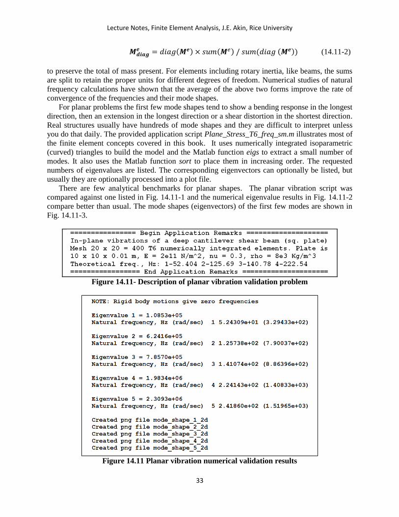
𝑴𝒅𝒊𝒂𝒈𝒆 = 𝑑𝑖𝑎𝑔(𝑴𝒆) × 𝑠𝑢𝑚(𝑴𝑒) / 𝑠𝑢𝑚(𝑑𝑖𝑎𝑔 (𝑴𝒆)) (14.11-2)
to preserve the total of mass present. For elements including rotary inertia, like beams, the sums
are split to retain the proper units for different degrees of freedom. Numerical studies of natural
frequency calculations have shown that the average of the above two forms improve the rate of
convergence of the frequencies and their mode shapes.
For planar problems the first few mode shapes tend to show a bending response in the longest
direction, then an extension in the longest direction or a shear distortion in the shortest direction.
Real structures usually have hundreds of mode shapes and they are difficult to interpret unless
you do that daily. The provided application script Plane_Stress_T6_freq_sm.m illustrates most of
the finite element concepts covered in this book. It uses numerically integrated isoparametric
(curved) triangles to build the model and the Matlab function eigs to extract a small number of
modes. It also uses the Matlab function sort to place them in increasing order. The requested
numbers of eigenvalues are listed. The corresponding eigenvectors can optionally be listed, but
usually they are optionally processed into a plot file.
There are few analytical benchmarks for planar shapes. The planar vibration script was
compared against one listed in Fig. 14.11-1 and the numerical eigenvalue results in Fig. 14.11-2
compare better than usual. The mode shapes (eigenvectors) of the first few modes are shown in
Fig. 14.11-3.
Figure 14.11- Description of planar vibration validation problem
Figure 14.11 Planar vibration numerical validation results

Lecture Notes, Finite Element Analysis, J.E. Akin, Rice University
34
Figure 14.11-5 First five modes of planar vibration validation problem
14.12 Acoustical vibrations:
14.13 Principal stresses: At any point in a stressed solid there are three mutually
orthogonal planes where the shear stresses vanish and only the normal stresses remain. Those
three normal stresses are called the principal stresses. The principal stresses are utilized to define
the most common failure criteria theories for most materials. Therefore, their calculation is
usually obtained at each quadrature point in a stress analysis. The principal stresses are found
from a small 𝟑 × 𝟑 classic eigen-problem:
|[𝝈] − 𝜆𝑘[𝑰]| = 0, 𝑘 = 1, … , 𝑛𝑠 (14.13-1)
where [𝑰] is the identity matrix, [𝝈] is the symmetric second order stress tensor, 𝜆𝑘, is a real
principal stress value giving the algebraic maximum stress, 𝜆1 = 𝜎1, the minimum stress 𝜆2 =𝜎2, and for three-dimensional solids 𝜆3 = 𝜎3 the intermediate stress. (This process is valid for
any other second order symmetric tensor, such as the moment of inertia tensor.) The principle
stresses (in reverse order) are obtained from the Matlab function eig, with only [𝝈] as the single

Lecture Notes, Finite Element Analysis, J.E. Akin, Rice University
35
argument. Finite element formulations often use the Voigt stress notation as a condensed form of
the stress tensor:
𝝈𝑇 = [𝜎𝑥 𝜎𝑦 𝜎𝑧 𝜏𝑥𝑦 𝜏𝑥𝑧 𝜏𝑦𝑧] ⇔ [𝝈] = [
𝜎𝑥𝑥 𝜏𝑥𝑦 𝜏𝑥𝑧
𝜏𝑥𝑦 𝜎𝑦𝑦 𝜏𝑦𝑧
𝜏𝑥𝑧 𝜏𝑦𝑧 𝜎𝑧𝑧
]
The principal stresses define other physically important quantities, such the measure of
material failure by the distortional energy criterion:
𝜎𝐸 =1
√2√(𝜎1 − 𝜎2)2 + (𝜎1 − 𝜎3)2 + (𝜎2 − 𝜎3)2 (14.14-2)
…𝜎𝐸 =1
√2√(𝜎𝑦𝑦 − 𝜎𝑥𝑥)
2+ (𝜎𝑧𝑧 − 𝜎𝑥𝑥)
2 + (𝜎𝑧𝑧 − 𝜎𝑦𝑦)2+ 6(𝜏𝑥𝑦
2 + 𝜏𝑥𝑧2 + 𝜏𝑦𝑧
2) (14.14-3)
which has the units of stress, but is not a physical stress. That measure is called the Equivalent
stress or the Von Mises stress.
Another terminology is the ‘stress intensity’ is defined as 𝜎𝐼 = 𝜎1 − 𝜎2 = 2𝜏𝑚𝑎𝑥 where
𝜏𝑚𝑎𝑥 is the absolute maximum shear stress on any plane in the solid at that point. There is also a
simple mathematical upper bound for the maximum shear stress: 𝜏𝑙𝑖𝑚𝑖𝑡 = 𝜎𝐸/√3. For plane-
stress problems it is common to find the maximum in plane shear stress from
𝜏𝑝𝑙𝑎𝑛𝑒 = √(𝜎𝑥−𝜎𝑦)
2
2
+ 𝜏𝑥𝑦2 ≤ 𝜏𝑚𝑎𝑥 =
1
2(𝜎1 − 𝜎3) (14.14-4)
But, if the thickness of the planar part is not very small the absolute maximum shear stress can
lie in a different plane and has to be found from the above three-dimensional calculation.
For a ductile material, its yield stress, 𝜎𝑌, is compared to the 𝜎𝐸 value to see if it has failed
based on distortional energy at the point. Material failure is declared when 𝜎𝐸 ≥ 𝜎𝑌. That is
checked because in a uniaxial tension test of material failure
𝜎𝑡𝑒𝑠𝑡 =1
√2√(𝜎𝑦 − 0)
2+ (𝜎𝑦 − 0)
2+ (0 − 0)2 =
√2
√2𝜎𝑦 = 𝜎𝑦
The yield stress of a ductile material is also compared to the stress intensity because in a uniaxial
tension test of material failure the maximum shear stress is 𝜏𝑚𝑎𝑥 = 𝜎𝑌 2⁄ and the Intensity
measure becomes
𝜎𝑡𝑒𝑠𝑡 = 𝜎𝑌 − 0 = 2𝜏𝑚𝑎𝑥.
Example 14.14-1 Given: The stress at a point is
𝝈𝑇 = [1 1 4 −3 √2 −√2] ⇔ [𝝈] = [ 1 −3 √2
−3 1 −√2
√2 −√2 4
] MPa
Develop a Matlab script to determine the principal stresses, the intensity, and the equivalent
stress. Solution: The script in Fig. 14.14-1 gives principal stresses of 𝜎(1: 3) = [6, 2, −2] MPa,
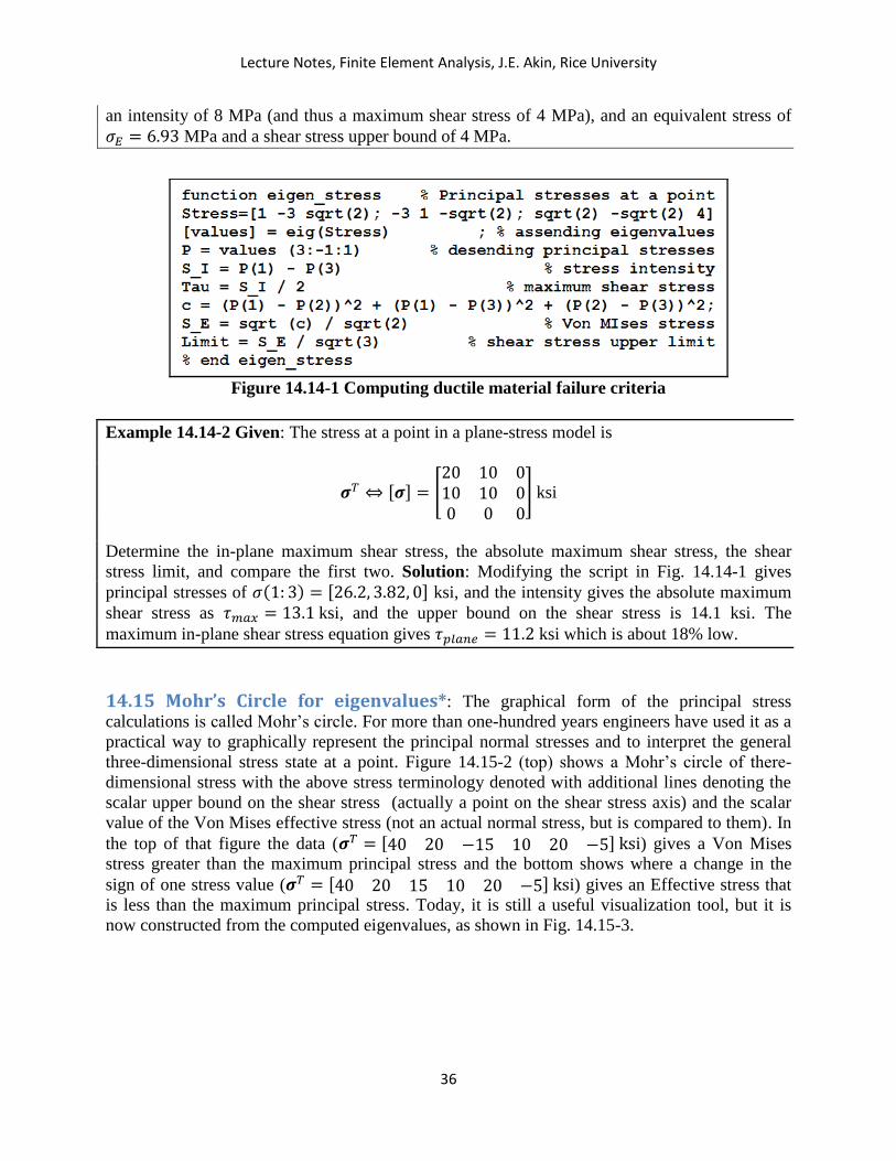
Lecture Notes, Finite Element Analysis, J.E. Akin, Rice University
36
an intensity of 8 MPa (and thus a maximum shear stress of 4 MPa), and an equivalent stress of
𝜎𝐸 = 6.93 MPa and a shear stress upper bound of 4 MPa.
Figure 14.14-1 Computing ductile material failure criteria
Example 14.14-2 Given: The stress at a point in a plane-stress model is
𝝈𝑇 ⇔ [𝝈] = [20 10 010 10 00 0 0
] ksi
Determine the in-plane maximum shear stress, the absolute maximum shear stress, the shear
stress limit, and compare the first two. Solution: Modifying the script in Fig. 14.14-1 gives
principal stresses of 𝜎(1: 3) = [26.2, 3.82, 0] ksi, and the intensity gives the absolute maximum
shear stress as 𝜏𝑚𝑎𝑥 = 13.1 ksi, and the upper bound on the shear stress is 14.1 ksi. The
maximum in-plane shear stress equation gives 𝜏𝑝𝑙𝑎𝑛𝑒 = 11.2 ksi which is about 18% low.
14.15 Mohr’s Circle for eigenvalues*: The graphical form of the principal stress
calculations is called Mohr’s circle. For more than one-hundred years engineers have used it as a
practical way to graphically represent the principal normal stresses and to interpret the general
three-dimensional stress state at a point. Figure 14.15-2 (top) shows a Mohr’s circle of there-
dimensional stress with the above stress terminology denoted with additional lines denoting the
scalar upper bound on the shear stress (actually a point on the shear stress axis) and the scalar
value of the Von Mises effective stress (not an actual normal stress, but is compared to them). In
the top of that figure the data (𝝈𝑇 = [40 20 −15 10 20 −5] ksi) gives a Von Mises
stress greater than the maximum principal stress and the bottom shows where a change in the
sign of one stress value (𝝈𝑇 = [40 20 15 10 20 −5] ksi) gives an Effective stress that
is less than the maximum principal stress. Today, it is still a useful visualization tool, but it is
now constructed from the computed eigenvalues, as shown in Fig. 14.15-3.

Lecture Notes, Finite Element Analysis, J.E. Akin, Rice University
37
Figure 14.15-2 Mohr’s circles where 𝝈𝑬 > 𝝈𝟏 (top) and 𝝈𝑬 < 𝝈𝟏

Lecture Notes, Finite Element Analysis, J.E. Akin, Rice University
38
Figure 14.15-3 Mohr’s circles of stress from stress tensor eigenvalues
14.16 Time Independent Schroedinger Equation* (TISE): The TISE is very important
in quantum mechanics. It is a wave equation in terms of a waveform, Ψ, and the system energy,
E, which predicts the probability of the distribution of an event or an outcome. The complex
time dependent Schroedinger equation is
−h2
2𝑚∇2𝜓(𝒓, 𝑡) + 𝑉(𝒓)𝜓(𝒓, 𝑡) = 𝑖h
𝜕
𝜕𝑡𝜓(𝒓, 𝑡)
For a harmonic oscillator, 𝜓(𝒓, 𝑡) = Ψ(𝐫)𝑒−𝑖𝜔𝑡. Substituting that yields the time independent
form
−h2
2𝑚∇2Ψ(𝐫) + 𝑉(𝒓)Ψ(𝐫) = h ω 𝜓(𝒓, 𝑡) = E Ψ(𝐫)
Here h is the reduced Planck constant, 𝑚 is the particle mass, ω is the frequency of vibration,
and V is the Potential Energy. For a one-dimensional quantum harmonic oscillator the form of
the Hamiltonian operator is
𝐻(𝑥) = −h2
2𝑚
𝜕2
𝜕𝑥2 +1
2𝑘𝑥2.
The operator on the left is the Hamiltonian, H(𝒓), and the TISE is often written as
H(𝒓)Ψ(𝐫) = E Ψ(𝐫)
The TISE is an eigenvalue problem with eigenvalues 𝐸𝑘 and the corresponding
eigenvectorsΨ𝑘. For bound states the eigenvalues are discrete and easily calculated by the finite
element method. In quantum mechanics the eigenvalues are desired to be accurate to at least one

Lecture Notes, Finite Element Analysis, J.E. Akin, Rice University
39
part in 1012. The waveform (eigenvector) is an infinitely differentiable (𝐶∞) function which
rapidly oscillates with a decreasing period.
Using typical element interpolation functions gives the matrix form [𝑺 − 𝐸𝑘 𝑴]{𝚿𝒌} = {𝟎} which becomes the general matrix eigen-problem
|𝑺 − 𝐸𝑘 𝑴| = 0
Applying 𝐶0Lagrangian interpolation methods has required as many as 40,000 DOF to reach an
acceptable accuracy. Since the waveform is 𝐶∞, it makes sense to employ elements with at least
slope and curvature continuity. For one-dimensional elements the Hermite family of
interpolations easily give 𝐶𝑛 interpolations when (𝑛 + 1) DOF per node are used. Also, 𝐶𝑛
rectangular elements can be formed from tensor products of the one-dimensional Hermite
elements. The domains are typically semi-infinite so geometric errors at the boundary are less
important. Triangular and solid elements are desirable for the TISE but it is very difficult to
obtain even 𝐶1elements in those forms. There the isogeometric elements seem like a natural
choice since they can easily yield at least 𝐶2 interpolations.

Lecture Notes, Finite Element Analysis, J.E. Akin, Rice University
40
14.17 Summary PDE Eigenvalue Form: ∇𝟐𝑢(𝑥, 𝑦, 𝑡) + 𝜆 𝑢(𝑥, 𝑦, 𝑡) = 0
Interpolation: 𝑢(𝑥) = 𝑯(𝑟) 𝒖𝒆
Matrix form: det [𝑲 + 𝜆 𝑴] = |𝑲 + 𝜆𝑴| = 0
Eigen-group: [K + λj M]δj = 0, j = 1, 2, …
Iron’s Bound Theorem: 𝜆𝑚𝑖𝑛𝑒 ≤ 𝜆𝑚𝑖𝑛 ≤ 𝜆𝑚𝑎𝑥 ≤ 𝜆𝑚𝑎𝑥
𝑒
Vibration: λ = ω2, ω real
Rigid body motion: ω = 0
Spring-mass: 𝜔 = √𝑘 𝑚⁄
Stiffnesses: 𝑲𝑬 = elastic, 𝑲𝒌
= foundation stiffness, 𝑲𝑮 = geometric stiffness
Buckling: [𝑲𝑬 + 𝑲𝒌
+ 𝐵𝐿𝐹 𝑲𝑮]𝜹 = 𝟎
Beam-Column: |(𝑲𝑬 + 𝑁𝐵𝑲𝒏
) − 𝜔2𝑴| = 0, 𝑲𝑮 = 𝑁𝐵𝑲𝒏
Lagrange linear line element stiffness matrix:
𝑲𝒆𝒃𝒂𝒓 =
𝐸𝑒𝐴𝑒
𝐿𝑒[ 1 −1−1 1
] , 𝑲𝒆𝒔𝒉𝒂𝒇𝒕 =
𝐺𝑒𝐽𝑒
𝐿𝑒[ 1 −1−1 1
] , 𝑲𝒆𝒔𝒑𝒓𝒊𝒏𝒈 = 𝑘𝑒 [
1 −1−1 1
]
Lagrange quadratic line element stiffness matrix:
𝑲𝒆𝒃𝒂𝒓 =
𝐸𝑒𝐴𝑒
3 𝐿𝑒 [ 7 −8 1−8 16 −8 1 −8 7
]
Lagrange cubic line element stiffness matrix:
𝑲𝒆𝒃𝒂𝒓 =
𝐸𝑒𝐴𝑒
40𝐿𝑒 [
148 −189−189 432
54 −13−297 54
54 −297 −13 54
432 −189 −189 148
]
Lagrange linear line element consistent mass matrix: 𝑴𝒆 =𝑚𝑒
6[2 11 2
]
Lagrange quadratic line element consistent mass: 𝑴𝒆 =𝑚𝑒
30[
4 2 −1 2 16 2−1 2 4
]

Lecture Notes, Finite Element Analysis, J.E. Akin, Rice University
41
Lagrange cubic line element consistent mass matrix: 𝑴𝒆 =𝑚𝑒
1680 [
128 99 99 648
−36 19−81 −36
−36 −81 19 −36
648 99 99 128
]
Lagrange linear triangle consistent mass matrix: 𝑴𝒙𝒆 =
𝑚𝑒
12[2 1 11 2 11 1 2
] = 𝑴𝒚𝒆
𝑴𝒆(𝑶𝒅𝒅,𝑶𝒅𝒅) = 𝑴𝒙𝒆, 𝑴𝒆(𝑬𝒗𝒆𝒏,𝑬𝒗𝒆𝒏) = 𝑴𝒚
𝒆
Lagrange linear line element averaged mass matrix: 𝑴𝒆 =𝑚𝑒
12 [5 11 5
]
Lagrange quadratic line averaged mass: 𝑴𝒆 =𝑚𝑒
60[ 9 2 −1 2 36 2−1 2 9
]
Lagrange cubic line averaged mass matrix: 𝑴𝒆 =𝑚𝑒
325920 [
25856 96039603 130896
−3492 1843−7857 −3492
−3492 −78571843 −3492
130896 96039603 25856
]
Lagrange linear triangle averaged mass matrix: 𝑴𝒙𝒆 =
𝑚𝑒
24 [6 1 11 6 11 1 6
] = 𝑴𝒚𝒆
𝑴𝒆(𝑶𝒅𝒅,𝑶𝒅𝒅) = 𝑴𝒙𝒆 , 𝑴𝒆(𝑬𝒗𝒆𝒏, 𝑬𝒗𝒆𝒏) = 𝑴𝒚
𝒆
Lagrange linear line element diagonalized mass matrix: 𝑴𝒆 =𝑚𝑒
2[1 00 1
]
Lagrange quadratic line diagonalized mass: 𝑴𝒆 =𝑚𝑒
6[1 0 00 4 00 0 1
]
Lagrange cubic line element diagonalized mass matrix : 𝑴𝒆 =𝑚𝑒
194 [
16 0 0 81
0 00 0
0 00 0
81 0 0 16
]
Lagrange linear triangle diagonalized mass matrix: 𝑴𝒙𝒆 =
𝑚𝑒
3[1 0 00 1 00 0 1
] = 𝑴𝒚𝒆
𝑴𝒆(𝑶𝒅𝒅,𝑶𝒅𝒅) = 𝑴𝒙𝒆 , 𝑴𝒆(𝑬𝒗𝒆𝒏, 𝑬𝒗𝒆𝒏) = 𝑴𝒚
𝒆

Lecture Notes, Finite Element Analysis, J.E. Akin, Rice University
42
14.18 Exercises
1. Repeat the prior guitar string frequency study to obtain an estimate of the first two smallest
frequencies and their relative mode shapes by using three two-node linear elements. (Ans:
𝜔1 = 3.2863 √𝑇 𝜌𝐿2⁄ , 𝜔2 = 7.3485 √𝑇 𝜌𝐿2⁄ )
2. Given the stress tensor at a point in a ductile material of [𝝈] = [40 10 2010 20 −520 −5 −15
] MPa,
determine the maximum compression (-) stress and the limit on the maximum shear stress.
(Ans: -23.0, 36.1 MPa)
3. Use a quadratic line element with the consistent mass matrix to find the first two frequency
estimates for the axial vibration of a bar and give their percent error (see Ex. 14.4-3). (Ans: %,
%)
4. Use a quadratic line element with its diagonalized mass matrix to find the first two frequency
estimates for the axial vibration of a bar and give their percent error (see Ex. 14.4-3). (Ans: %,
%)
5. For the simple truss in Fig. 14.8-2 determine the critical buckling value if the compressive
force at node 1 is horizontal (see Ex. 14.8-2).
6. For the simple truss in Fig. 14.8-2 determine the critical buckling value if the compressive
force at node 1 has a slope of 4 horizontal to 3 vertical (see Ex. 14.8-2).
Index abs, 28 absolute maximum shear stress, 35 acoustical pressure, 4 acoustical vibration, 1 adaptive mesh, 17 anti-symmetric mode, 7, 17 averaged mass matrix, 4, 11 axial vibration, 11 beam vibration, 12 beam with axial load, 28 bending stiffness, 15 BHA, 11 BLF, 22 bottom hole assembly, 11 buckled mode shape, 23, 27 buckled shape, 4 buckling, 4, 21 buckling factor, 4 buckling load factor, 22 cantilever beam, 15 catastrophic failure, 21, 23 centripetal force, 29 characteristic equation, 11
column, 22, 28 column buckling, 29 consistent mass matrix, 4, 7, 10, 12, 16 cubic beam, 25, 29 curvature continuity, 39 degrees of freedom, 2 determinant, 4 diag, 2, 27 diagonal mass matrix, 5 diagonalized mass matrix, 4 direction angles, 24 disk, 12 disp, 13 distortional energy criterion, 35 drill string, 11 ductile material, 35 eig, 2, 13, 34, 36 eig.m, 9 eigen-problem, 1, 4 eigenvalue, 4, 10, 26 eigenvalues, 38 eigenvector, 4, 39 eigs, 2
Lecture Notes, Finite Element Analysis, J.E. Akin, Rice University
43
elastic support, 15 equation of motion, 11 equivalent stress, 35 extreme eigenvalues, 3 Factor of Safety, 23, 28 failure criteria, 34 fixed–pinned beam, 25 fixed-pinned column, 29 for, 13 FOS, 28 free unknowns, 4 generalized mass matrix, 3 geometric stiffness matrix, 4, 23, 24, 25, 28 get_and_add_pt_mass.m, 6 get_and_add_pt_stiff.m, 6 global constant, 3 governing matrix system, 7 handbook solution, 6 harmonic oscillator, 38 Helmholtz equation, 1, 7 Hermite interpolation, 7, 39 hyperbolic equation, 6 infinite gradient, 17 initial stress matrix, 4 initial stress stiffness, 24 integration by parts, 7 interpolation functions, 7 Iron's Theorem, 3 isogeometric elements, 39 L2_C0, 7 L2_C1, 7, 12 L3_C0, 7, 8, 9, 10 L3_C1, 12 largest eigenvalue, 3 linear buckling, 23 load case, 22 L-shaped membrane, 16, 17 mass density, 6, 11 mass matrix, 28 massless spring, 5 material failure, 35 Matlab logo, 16 maximum principal stress, 36 maximum shear stress, 35 member rotation matrix, 24 membrane stiffness matrix, 16 membrane tension, 16 membrane thickness, 16
membrane vibration, 16 Membrane_vibration.m, 17 mesh control, 17 min, 2, 28 mode shape, 7, 9 mode_shape_surface.m, 17 Mohr’s circle, 36 moment of inertia, 12 msh_mass_pt.txt, 6 msh_stiff_pt.txt, 6 natural frequency, 4, 8, 28 Newton’s law, 12 nonessential boundary condition, 12 normalized eigenvector, 4 point inertia, 12 point mass, 5, 11 point spring, 5 point stiffness, 5 polar moment of inertia, 11 post-buckling, 23 principal stress, 36 principal stresses, 34 propped cantilever, 15 Q4_C0, 17 Q9_C0, 17 quadrature point, 34 quantum mechanics, 38 quintic beam, 25 radius of gyration, 24 real, 2, 13 rectangular element, 39 re-entrant corner, 17 rigid body motion, 2 rotational inertia, 11 rotational pendulum, 12 rotational spring, 15 Schroedinger equation, 38 second order tensor, 34 shear modulus, 11 SHM, 6 simple harmonic motion, 6 singular point, 17 singularity element, 17 slenderness ratio, 24 slope continuity, 7 smallest eigenvalue, 3 sort, 3 sound system, 1
Lecture Notes, Finite Element Analysis, J.E. Akin, Rice University
44
spring-mass system, 5 sqrt, 10, 36 stiffness matrix, 3, 10 stress intensity, 35 stress stiffening, 4 stress tensor, 34 stress-strain relation, 23 string frequency, 42 string tension, 8 string vibration, 6 String_vib_2_L3.m, 9 structural instability, 21 structural stiffness matrix, 4 symmetric mode, 7, 17 tension, 6 TISE, 38 torsional shaft, 11 torsional stiffness, 11
torsional stiffness matrix, 11 torsional vibration, 11, 13 Torsional_Vib_BHA_L3.m, 12 transverse displacement, 16 transverse spring, 26 truss buckling, 24 turbine blade, 29 uniaxial tension test, 35 validation, 6 vector subscripts, 13 vibration, 2 Von Mises stress, 35 wave equation, 6, 38 waveform, 38 waveguide, 1 yield stress, 23, 35 zeros, 10