Page 1 of 9

Mech 403 Equilibrium Diagram Assignment J.E. Akin, Rice University

A review of prior design reports showed that most obvious errors occurred because the analysis failed to include a

structural equilibrium Free Body Diagram (FBD) or a thermal equilibrium Energy Balance Diagram (EBD). Therefore, each

student is required to submit one FBD or EBD, to also be included in the design report, for a part or assembly used in

their design. I will review the first submission and discuss it with you, if necessary. The second submission will be

graded and will represent 5% of the course grade.

The concept of a force equilibrium FBD addresses a part or an assembly that is loaded by external forces and subject to

displacement constraints. The displacement constraints introduce unknown reaction forces. The FBD isolates the part

or assembly from its surroundings and shows all the force and moments acting upon it, both loadings and reactions.

Then the condition of equilibrium is imposed to determine all of the forces. For simple systems Newton’s equations of

motion are sufficient to find all the unknown forces. However, most equilibrium problems are statically indeterminate.

That requires that some displacements must be solved to satisfy equilibrium, and to find the reaction forces. A finite

cement simulation always computes the system displacements and reaction forces needed to satisfy equilibrium.

There are fairly common uses of static and dynamic FBDs (presented at the end of this review), but the use of EBDs is far

less common. For thermal equilibrium diagrams there does not seem to be a set of standard symbols. Thus, the analyst

picks their own symbols to represent the physical problem.

Here, an example problem reviews the thermal balance diagram concepts. In a thermal FE simulation the essential

boundary condition is prescribed temperatures. By default, all surfaces in a thermal FE study are insulated (have no

crossing heat flow) unless the user specifies otherwise. A known internal rate of heat generation per unit volume

(thermal power), known heat flux across a boundary, convection at a surface, and radiation at a surface are thermal

loads. After the temperatures everywhere are computed, to satisfy thermal equilibrium, then the thermal reaction heat

flows can be found for regions of prescribed temperatures. (In SolidWorks, go to Results List heat flows select

prescribed temperature region.) The reaction heat flow in and/or out, the internal heat generated, and the specified

heat flows will balance.

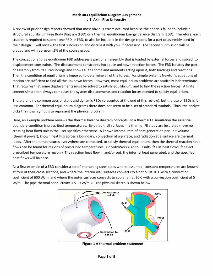
As a first example of a EBD consider a set of interacting steel pipes where (assumed) constant temperatures are known

at four of their cross-sections, and where the interior wall surfaces convects to a hot oil at 70 C with a convection

coefficient of 600 W/m, and where the outer surfaces convects to cooler air at 30 C with a convection coefficient of 5

W/m. The pipe thermal conductivity is 51.9 W/m-C. The physical sketch is shown below.

Figure 1 A thermal problem statement

Page 2 of 9

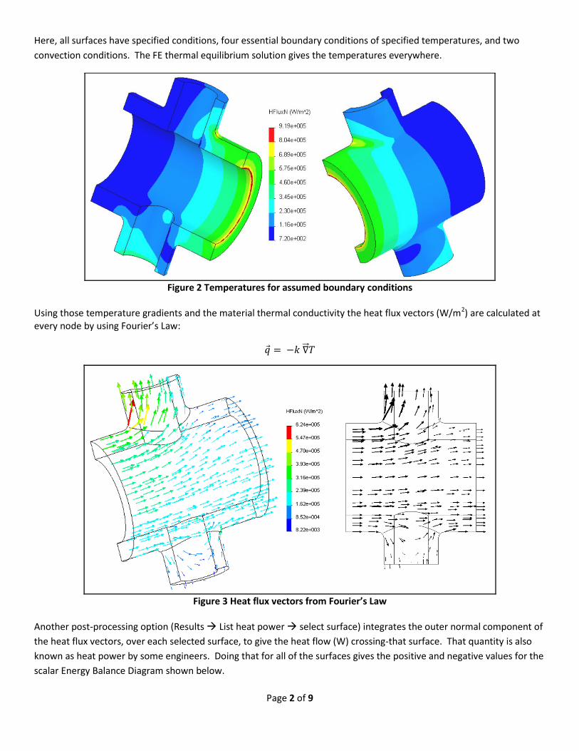
Here, all surfaces have specified conditions, four essential boundary conditions of specified temperatures, and two

convection conditions. The FE thermal equilibrium solution gives the temperatures everywhere.

Figure 2 Temperatures for assumed boundary conditions

Using those temperature gradients and the material thermal conductivity the heat flux vectors (W/m2) are calculated at every node by using Fourier’s Law:

�⃗� = −𝑘 ∇⃗⃗⃗𝑇

Figure 3 Heat flux vectors from Fourier’s Law

Another post-processing option (Results List heat power select surface) integrates the outer normal component of

the heat flux vectors, over each selected surface, to give the heat flow (W) crossing-that surface. That quantity is also

known as heat power by some engineers. Doing that for all of the surfaces gives the positive and negative values for the

scalar Energy Balance Diagram shown below.

Page 3 of 9

𝐻𝑒𝑎𝑡 𝑓𝑙𝑜𝑤 = ∫ �⃗� ∙ �⃗⃗�

𝑆

𝑑𝑆

Figure 4 Example Energy Balance Diagram

(integral of normal heat flux)

Energy in + Energy generated = Energy out (Conduction in) + (Convection in) + (Internal heat generated) = (Conduction out) + (Convection out)

(3,710 W + 566 W) + (0) +(0) = (270 W +310 W) + (3,642 W + 54 W) 4,276 W = 4,276 W

The conduction surface heat powers are what are necessary to maintain the specified essential boundary condition (the

known temperatures) on that surface. The convection surface heat powers are the amount of heat supplied or removed

by the surrounding fluid. (A similar statement applies to any radiation surfaces.)

If convection had not been specified then thus surfaces default to insulated surfaces, in a FE thermal model. That is, by

definition no heat flow crosses them. There the problem statement becomes

Figure 5 Problem statement for insulated surface assumptions

The computed FE thermal equilibrium temperatures become almost linear along each pipe segment:

Page 4 of 9

Figure 6 Temperatures for assumed insulated internal and external surfaces

Post-processing the temperatures to get the heat flux vectors and integrating their normal component over the surfaces

gives the surface heat flow (heat power) values needed to draw the EBD of Figure 7. Note that if the surfaces are

insulated much less heat power (1,684 W) is required to maintain the 400 C boundary condition than in the prior

example (3,710 W).

Figure 7 Energy Balance Diagram II

Energy in + Energy generated = Energy out

(Conduction in) + (Convection in) + (Internal heat generated) = (Conduction out) + (Convection out) (1,684 W + 16 W) + (0) + (0) = (1,140 W + 560 W) + (0)

1,700 W = 1,700 W

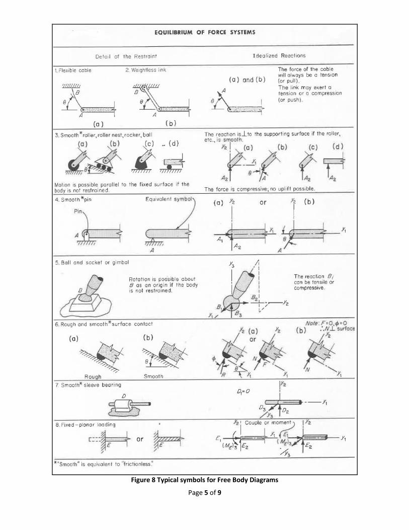
The use of FBDs for static equilibrium was introduced in introductory physics, and repeated in the sophomore

statics/dynamics class and the mechanics of solids class. For force FBDs there are a number of standard graphical

symbols, or icons, used to denote the types of displacement supports that are common. Several such symbols are

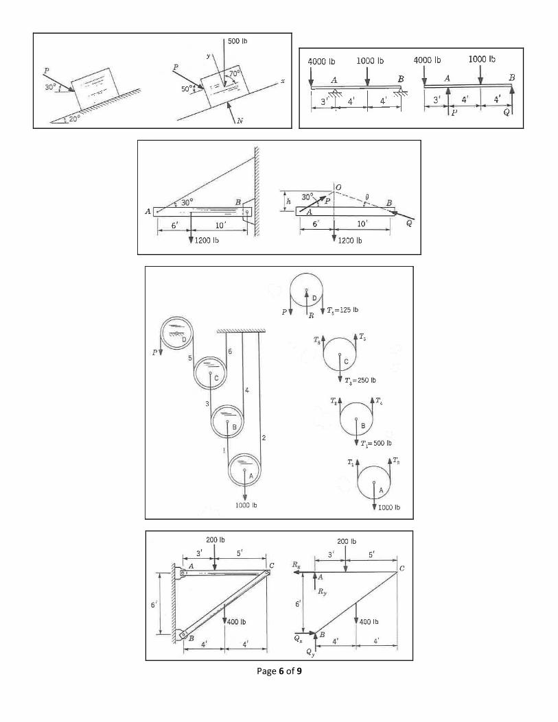
tabulated in the Figure 8. Several force FBD’s, from C.O. Harris “Mechanics for Engineers” are shown for review.

Page 5 of 9

Figure 8 Typical symbols for Free Body Diagrams

Page 6 of 9

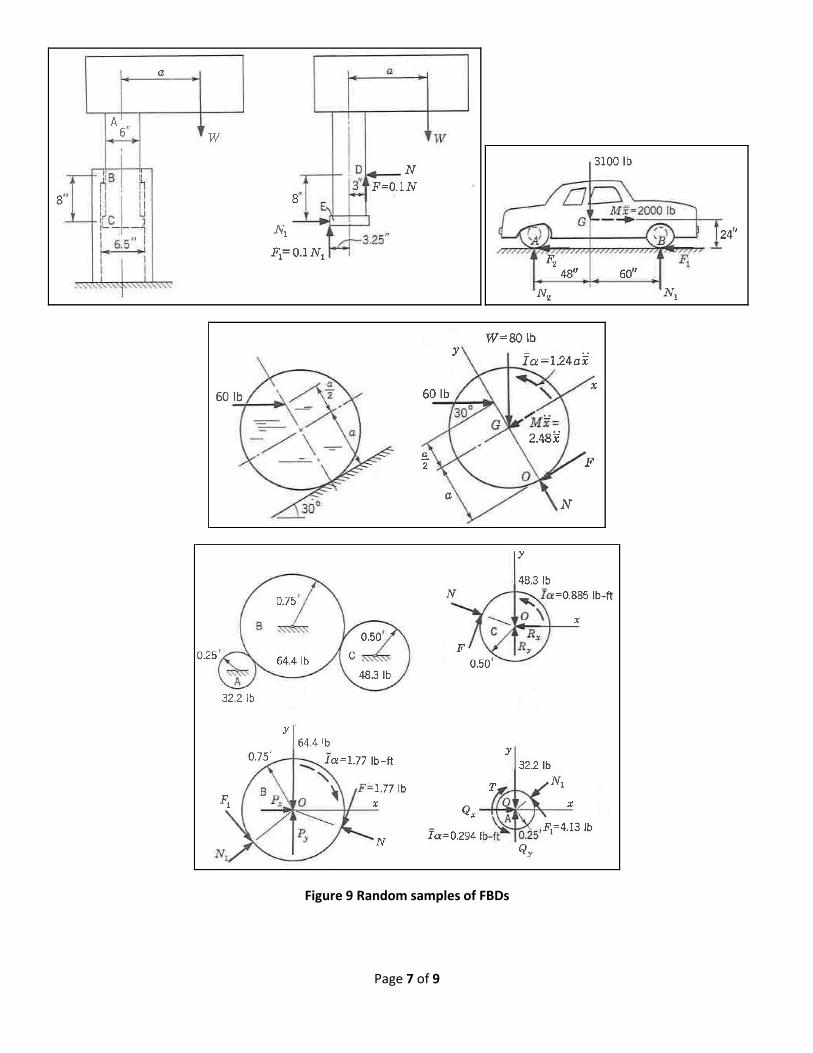
Page 7 of 9

Figure 9 Random samples of FBDs

Page 8 of 9

The image below in Figure 10 shows a bicycle front wheel brake assembly (from Norton, “Machine Design”). A FBD of

the front most member is shown in the following figure. That author choses to measure distances from the part center

of mass and to split all forces into orthogonal components. Most analysts tend to measure distances from a geometric

landmark, such as a circle center or one end of a member.

Figure 10 A problem statement sketch

Page 9 of 9

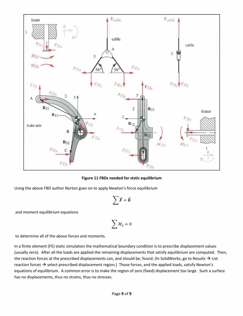
Figure 11 FBDs needed for ststic equilibrium

Using the above FBD author Norton goes on to apply Newton’s force equilibrium

∑ �⃗⃗⃗� = �⃗⃗⃗�

and moment equilibrium equations

∑ 𝑀𝑧 = 0

to determine all of the above forces and moments.

In a finite element (FE) static simulation the mathematical boundary condition is to prescribe displacement values

(usually zero). After all the loads are applied the remaining displacements that satisfy equilibrium are computed. Then,

the reaction forces at the prescribed displacements can, and should be, found. (In SolidWorks, go to Results List

reaction forces select prescribed displacement region.) Those forces, and the applied loads, satisfy Newton’s

equations of equilibrium. A common error is to make the region of zero (fixed) displacement too large. Such a surface

has no displacements, thus no strains, thus no stresses.