lecture notes, finite element analysis, j.e. akin, rice ... notes, finite element analysis, j.e....

Lecture Notes, Finite Element Analysis, J.E. Akin, Rice University

1

13. Elasticity .................................................................................................................................................. 1

13.1 Introduction ...................................................................................................................................... 1

13.2 Linear springs .................................................................................................................................... 4

13.3 Mechanical Work .............................................................................................................................. 6

13.5 Strain energy ..................................................................................................................................... 9

13.6 Material properties ......................................................................................................................... 10

13.7 Simplified elasticity models* .......................................................................................................... 12

13.8 Interpolating displacement vectors ................................................................................................ 16

13.9 Mechanical work in matrix form ..................................................................................................... 18

13.10 The Strain-Displacement Matrix ................................................................................................... 19

13.11 Stiffness matrix ............................................................................................................................. 22

13.12 Work done by initial strains .......................................................................................................... 22

13.13 Matrix equilibrium equations ....................................................................................................... 23

13.14 Symmetry and anti-symmetry ...................................................................................................... 29

13.15 Plane stress analysis ...................................................................................................................... 23

13.16 Axisymmetric stress analysis ......................................................................................................... 24

13.17 Solid stress analysis ....................................................................................................................... 25

13.18 Kinetic energy ............................................................................................................................... 29

13.19 Summary ....................................................................................................................................... 32

13.20 Exercises ........................................................................................................................................ 36

13. Elasticity

13.1 Introduction: The subject of elasticity deals with the stress analysis applications where

the component returns to its original size and shape when the loads acting on the component. The

finite element method has proven to be a very practical process for any elasticity analysis. The

vast majority of finite element elasticity models utilize the displacements as the primary

unknowns. A general solid analysis requires three displacement components that lead to six

stress components. An elasticity analysis involves four major topics: the displacement

components, the six strain components obtained from the gradients of the displacement

components (known in solid mechanics as the strain-displacement relation), and the experimental

material property knowledge that relates the strain components to the stress components. It is

more common to state the material stress-strain law which is the inverse of the experimental

relation. After the displacements, are known they are post-processed to give the strains and


2

stresses. Once the strains and stresses are known they must be compared to an experimentally

established material failure criterion.

All stress analysis involves a solid object. Historically, many mathematical simplifications

have been developed to model common special shapes in order to avoid actual solid stress

analysis. They include bending of curved three-dimensional shells, axisymmetric solids, two-

dimensional plane-stress (where a plane is stress free as in Fig. 13.1-1), two-dimensional plane-

strain (where a plane is strain free), bending of two-dimensional flat plates, two-dimensional

torsion of non-circular shafts, one-dimensional torsion of circular shafts, bending of one-

dimensional beams, and finally one-dimensional axial bars. All of those special cases have a

different set of governing differential equations. However, they can all be solved by a single

finite element approach.

Figure 13.1-1 Plane stress is a special case of solid stress analysis

Today, it is practical to conduct a three-dimensional stress analysis, but it is not always the

most accurate, or the most efficient approach. For example, in certain cases thousands of solid

elements approximating a straight beam can be less accurate that tens of beam elements.

Whatever element type is used in an analysis, all finite element study results should be

independently validated by some handbook solution, and/or some simplified mathematical model

in an attempt to set upper and lower bounds for the answer of the actual problem being solved.

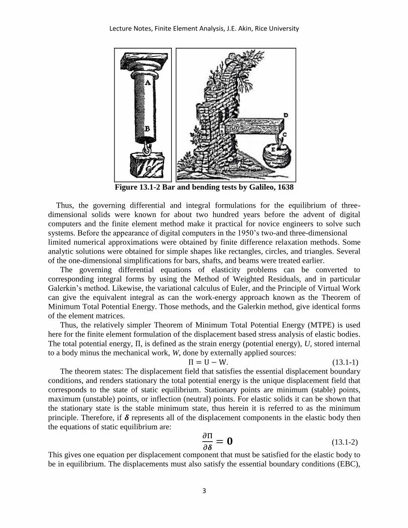
Early in human history people built with post, simple beams, and arches. One of the first

published studies of structures was that of Galileo in 1638 where he analyzed axial loads and the

bending of cantilever beams (see Fig. 13.1-2). His analysis was incorrect, but it represents the

beginning of engineers understanding of the mathematical analysis of structures. In 1678 Robert

Hooke published material studies that established the linear proportionality between material

strains and stresses. That relation was used as the foundation upon which the mechanics of

elastic structures was built. His work is often called Hooke’s law or the material constitutive law.

Sir Isaac Newton published his laws governing dynamics and equilibrium in 1687. With those

foundations Jacob Bernoulli almost correctly solved for the deflection of a cantilever beam in

1705. Leonard Euler correctly formulated the differential equations for beam equilibrium and

solved them in 1736. In 1744 Euler published the first book on variational calculus (which later

played a large part in finite element analysis). By 1750 the basic mechanics (materials and

differential equations) for treating the equilibrium and dynamics of all elastic structures were

known.


3

Figure 13.1-2 Bar and bending tests by Galileo, 1638

Thus, the governing differential and integral formulations for the equilibrium of three-

dimensional solids were known for about two hundred years before the advent of digital

computers and the finite element method make it practical for novice engineers to solve such

systems. Before the appearance of digital computers in the 1950’s two-and three-dimensional

limited numerical approximations were obtained by finite difference relaxation methods. Some

analytic solutions were obtained for simple shapes like rectangles, circles, and triangles. Several

of the one-dimensional simplifications for bars, shafts, and beams were treated earlier.

The governing differential equations of elasticity problems can be converted to

corresponding integral forms by using the Method of Weighted Residuals, and in particular

Galerkin’s method. Likewise, the variational calculus of Euler, and the Principle of Virtual Work

can give the equivalent integral as can the work-energy approach known as the Theorem of

Minimum Total Potential Energy. Those methods, and the Galerkin method, give identical forms

of the element matrices.

Thus, the relatively simpler Theorem of Minimum Total Potential Energy (MTPE) is used

here for the finite element formulation of the displacement based stress analysis of elastic bodies.

The total potential energy, Π, is defined as the strain energy (potential energy), U, stored internal

to a body minus the mechanical work, W, done by externally applied sources:

Π = U −W. (13.1-1)

The theorem states: The displacement field that satisfies the essential displacement boundary

conditions, and renders stationary the total potential energy is the unique displacement field that

corresponds to the state of static equilibrium. Stationary points are minimum (stable) points,

maximum (unstable) points, or inflection (neutral) points. For elastic solids it can be shown that

the stationary state is the stable minimum state, thus herein it is referred to as the minimum

principle. Therefore, if 𝜹 represents all of the displacement components in the elastic body then

the equations of static equilibrium are:

𝜕Π

𝜕𝜹= 𝟎 (13.1-2)

This gives one equation per displacement component that must be satisfied for the elastic body to

be in equilibrium. The displacements must also satisfy the essential boundary conditions (EBC),


4

and the above equations also yield the reactions needed for system equilibrium, developed at the

EBC locations.

13.2 Linear springs: Before considering the general case, a review of how these topics were

introduced in introductory physic courses. The ‘linear spring’ is usually introduced with the

essential boundary condition pre-applied by fixing one end against displacement. That reduces a

two degree of freedom (DOF) to a one DOF analysis, as noted in Fig. 13.1-2. The spring has an

axial stiffness of k. The unrestrained end has an axial force, F, that causes an axial displacement,

𝛿. If the system is in equilibrium what is the relation between these three features of the linear

spring?

Figure 13.1-2 Linear spring systems

Recall that the strain (potential) energy of a linear spring is 𝑈 = 𝑘 𝛿2/2. The mechanical

work due to the external force is defined as the product of the force and the displacement

component in the direction of the force. In this case, they are parallel so the mechanical work is

𝑊 = 𝛿 𝐹 In general, they are not parallel and the work is the scalar (dot) product of the force vector and

the displacement vector:

𝑊 = �⃗⃗� ∙ �⃗⃗� = 𝜹𝑻 𝑭 = 𝛿𝑥𝐹𝑥 + 𝛿𝑦𝐹𝑦 + 𝛿𝑧𝐹𝑧 (13.1-3)

Let the x-axis lie along the spring end points. Then the total potential energy is

Π(𝛿𝑥) = U −W = 𝑘 𝛿𝑥2/2 − 𝛿𝑥𝐹𝑥

Calculus teaches that to find a stationary points of a function y(x) it is necessary to set its

derivative to zero, 𝑑𝑦/𝑑𝑥 = 0, and solve that equation for the value of x that corresponds to the

stationary point. To determine what type of stationary point it is necessary to evaluate the second

derivative, 𝑑2𝑦 𝑑𝑥2⁄ , at the point. If the second derivative is positive it defines a minimum point,

if negative it defines a maximum point, and a zero value defines a neutral point.

The Total Potential Energy is defined as a function of each and every displacement unknown in

the system. Here, 𝛿𝑥 is the only displacement associated with the spring. Therefore, stationary

equilibrium for the spring requires 𝜕Π

𝜕𝛿𝑥= 0 = 2 𝑘 𝛿𝑥/2 − 𝐹𝑥

This gives the equilibrium equation as

𝛿𝑥 = 𝐹𝑥 𝑘 or ⁄ 𝐹𝑥 = 𝑘 𝛿𝑥

Physics courses usually state the second form. The deformed state minimizes the Total Potential

Energy as is seen by taking its second derivative: 𝑑2Π 𝑑𝛿𝑥2 = 𝑘⁄ , which is always positive.


5

Next, consider two identical springs joined in series. The mechanical work is still the same

since there is no external force applied to the intermediate node, 𝑊 = 0𝛿1 + 𝐹 𝛿2. There are

equal and opposite internal forces at that point. They are the reaction forces on the springs

needed to have each spring in equilibrium as well as having the assembly of springs in

equilibrium. The net displacement of the end where the external load is applied is (𝛿2 − 𝛿1), so

the scalar strain energy of the assembly of springs is

𝑈 =1

2𝑘𝛿1

2 +1

2𝑘(𝛿2 − 𝛿1)

2 =𝑘

2(2𝛿1

2 − 2𝛿1𝛿2 + 𝛿22)

and the Total Potential Energy becomes

Π =𝑘

2(2𝛿1

2 − 2𝛿1𝛿2 + 𝛿22) − (0𝛿1 + 𝐹 𝛿2)

To reach equilibrium, this quantity must be minimized with respect to each and every one of the

displacement degrees of freedom:

𝜕Π

𝜕𝛿1=𝑘

2(4𝛿1 − 2𝛿2) − (0)

𝜕Π

𝜕𝛿2=𝑘

2(−2𝛿1 + 2𝛿2) − (𝐹)

In matrix format the displacement based equations of equilibrium are

𝑘 [ 2 −1−1 1

] {𝛿1𝛿2} = {

0𝐹}

The leftmost node satisfied in advance the essential boundary condition of specifying a known

displacement (0 here), and these two displacement components will minimize the Total Potential

Energy (iff the square matrix is non-singular), and thus these displacements will correspond to

the state of static equilibrium. Multiplying by the inverse of the square matrix:

{𝛿1𝛿2} =

1

𝑘[1 11 2

] {0𝐹} =

𝐹

𝑘{12}

The left spring has the same displacement as it did in the previous case, 𝛿1 = 𝐹/𝑘, and the right

spring has a displacement that is twice as large 𝛿2 = 2𝐹/𝑘. This makes sense because the

external load, F, is simply transmitted through the first spring to the second spring which in turn

transmits it to rigid support wall.

Often the system reactions are needed, and sometimes the reactions on some or all of the

elements are needed. Since the EBC was applied in advance, there is no equation available to

compute the system reaction, but by requiring that each spring is in equilibrium the internal

reaction force(s) can be obtained since now all of the displacements are known. Let the reaction


6

force on the left node of the right spring be 𝑅, which is assumed to be in the positive direction.

The individual spring’s Total Potential Energy is

Π =1

2𝑘(𝛿2 − 𝛿1)

2 − (𝑅𝛿1 + 𝐹 𝛿2)

which gives the element equilibrium equations of

𝜕Π

𝜕𝛿1= 0 =

𝑘

2(2𝛿1 − 2𝛿2) − (𝑅)

𝜕Π

𝜕𝛿2= 0 =

𝑘

2(−2𝛿1 + 2𝛿2) − (𝐹)

and substituting all of the known displacements into the first element equilibrium equation gives

0 =𝑘

2(2𝐹/𝑘 − 4𝐹/𝑘) − (𝑅) = −𝐹 − 𝑅

which gives the expected (from Newton’s laws) result that 𝑅 = −𝐹.

13.3 Mechanical Work: To begin generalizing and automating the above process to any

elastic system it is necessary to consider additional types of external forces. A viscous fluid, and

other sources like electromagnetic surface eddy currents, can apply an external force per unit

area to adjacent solid surfaces. These are called ‘surface tractions’, and they are denoted in

vector and matrix forms by �⃗⃗� ↔ 𝑻, respectively. In this application the number of displacement

degrees of freedom at a point, 𝑛𝑔 is the same as the number of spatial dimensions, 𝑛𝑔 = 3 = 𝑛𝑠.

The differential force at a point on the surface area 𝑑𝑆 becomes 𝒅𝑭⃗⃗⃗⃗ ⃗ = �⃗⃗� 𝑑𝑆. When a point on the

surface, 𝑆, is subjected to a displacement, the scalar work done by the traction vector is

𝑑𝑊𝑇 = �⃗⃗� ∙ �⃗⃗� 𝑑𝑆 = 𝜹𝑇𝑻 𝑑𝑆

so that the total work done by all surface tractions is

𝑊𝑇 = ∫ 𝜹𝑇𝑻 𝑑𝑆

𝑆. (13.3-1)

Likewise, external translational acceleration and/or rotational velocities and accelerations,

and other sources like the effects of external magnetic fields acting on electric currents flowing

through a body, will cause forces per unit volume to occur inside an object. These are called

‘body forces’, and they are denoted in vector and matrix forms by �⃗� ↔ 𝒇, respectively, and the

differential force acting on a differential volume is 𝒅𝑭⃗⃗⃗⃗ ⃗ = �⃗� 𝑑𝑉. When the differential volume is

subjected to a displacement, the scalar work done by the body force vector is

𝑑𝑊𝑓 = �⃗⃗� ∙ �⃗� 𝑑𝑉 = 𝜹𝑇𝒇 𝑑𝑉

so that the total work done by all body forces is

𝑊𝑓 = ∫ 𝜹𝑇𝒇 𝑑𝑉

𝑉. (13.3-2)

Finally, recognizing that more than one point can have an external point load and that the

work done by each must be included the general definition of external mechanical work is


7

𝑊 = ∫ 𝜹𝑇𝒇 𝑑𝑉

𝑉+ ∫ 𝜹𝑇𝑻 𝑑𝑆

𝑆+ ∑ 𝜹𝑘

𝑇𝑭𝑘𝑘=𝑛𝑃𝑘=1 (13.3-3)

13.4 Displacements and mechanical strains: To generalize the strain energy definition it will

be defined for the full three-dimensional case so all of the simplifications, like plane stress case

in Fig. 13.1-1, are automatically included. The governing matrix relations to be developed in this

chapter retain their symbolic forms in all elasticity applications. They simply change size when

one of the simplifications is invoked. The starting point is the 𝑛𝑔 = 3 displacement components

in the x-, y-, and z-directions at a point:

�⃗⃗� ↔ 𝒖 = {

𝑢(𝑥, 𝑦, 𝑧)𝑣(𝑥, 𝑦, 𝑧)𝑤(𝑥, 𝑦, 𝑧)

} = 𝜹 .

(13.4-1)

The differential of the x-component of the displacement vector is

𝑑𝒖(𝑥, 𝑦, 𝑧) =𝜕𝑢

𝜕𝑥𝑑𝑥 +

𝜕𝑢

𝜕𝑦𝑑𝑦 +

𝜕𝑢

𝜕𝑧𝑑𝑧

The differential of the displacement vector can be written in matrix form as

𝑑𝒖 = {

𝑑𝑢(𝑥, 𝑦, 𝑧)

𝑑𝑣(𝑥, 𝑦, 𝑧)𝑑𝑤(𝑥, 𝑦, 𝑧)

} =

[ 𝜕𝑢

𝜕𝑥

𝜕𝑢

𝜕𝑦

𝜕𝑢

𝜕𝑧𝜕𝑣

𝜕𝑥

𝜕𝑣

𝜕𝑦

𝜕𝑣

𝜕𝑧𝜕𝑤

𝜕𝑥

𝜕𝑤

𝜕𝑦

𝜕𝑤

𝜕𝑧 ]

{𝑑𝑥𝑑𝑦𝑑𝑧

}

Notice that the square matrix containing the partial derivatives of the displacement components

can be written as the sum of three square matrices as:

[ 𝜕𝑢

𝜕𝑥0 0

0𝜕𝑣

𝜕𝑦0

0 0𝜕𝑤

𝜕𝑧 ]

+1

2

[ 0

𝜕𝑢

𝜕𝑦+

𝜕𝑣

𝜕𝑥

𝜕𝑢

𝜕𝑧+𝜕𝑤

𝜕𝑥

𝜕𝑣

𝜕𝑥+𝜕𝑢

𝜕𝑦0

𝜕𝑣

𝜕𝑧+𝜕𝑤

𝜕𝑦

𝜕𝑤

𝜕𝑥+𝜕𝑢

𝜕𝑧

𝜕𝑤

𝜕𝑦+𝜕𝑣

𝜕𝑧0 ]

+1

2

[ 0

𝜕𝑢

𝜕𝑦−

𝜕𝑣

𝜕𝑥

𝜕𝑢

𝜕𝑧−𝜕𝑤

𝜕𝑥

𝜕𝑣

𝜕𝑥−𝜕𝑢

𝜕𝑦0

𝜕𝑣

𝜕𝑧−𝜕𝑤

𝜕𝑦

𝜕𝑤

𝜕𝑥−𝜕𝑢

𝜕𝑧

𝜕𝑤

𝜕𝑦−𝜕𝑣

𝜕𝑧0 ]

.

These three groups of combinations of the displacement gradients have geometrical

interpretations and physical interpretations. The geometrical shapes for both the plane-stress and

the plane-strain simplifications of a planar rectangular differential element are shown in Fig.

13.4-1. The first matrix partition represents a displacement change of the faces of that element in

directions normal to their original positions (left part of the figure). Those diagonal components

are known as the ‘normal strains’:


8

휀𝑥 =𝜕𝑢

𝜕𝑥, 휀𝑦 =

𝜕𝑣

𝜕𝑦, 휀𝑧 =

𝜕𝑤

𝜕𝑧 (13.4-2)

Normal strains change the volume of the differential element but not its shape. The differential

element goes from one rectangle to another.

The second matrix of displacement gradient component combinations changes the shape

(middle of Fig. 13.4-1) by distorting the rectangle into a parallelogram, without changing its

area. This second symmetric matrix contains components of what mathematicians call the shear

strain tensor. However, engineers choose to define the terms inside the matrix brackets as the

(engineering) shear strains:

𝛾𝑥𝑦 =𝜕𝑢

𝜕𝑦+

𝜕𝑣

𝜕𝑥= 𝛾𝑦𝑥, 𝛾𝑥𝑧 =

𝜕𝑢

𝜕𝑧+𝜕𝑤

𝜕𝑥= 𝛾𝑧𝑥, 𝛾𝑦𝑧 =

𝜕𝑣

𝜕𝑧+𝜕𝑤

𝜕𝑦= 𝛾𝑧𝑦 (13.4-3)

The omission of the one-half term for the engineering shear strains simply means that the rules

for rotating the stresses (Mohr’s circle) and the engineering strains from one coordinate system

to another are different. That contrasts with the tensor formulations where the stress tensor and

the strain tensor (and any other second order tensor) have the same rotational transformation.

The third matrix corresponds to a rigid body rotation (right part of the figure) of the

differential element. That rotation does not change its volume and does not change its shape. In

other words, the third combination of displacement components has no effect on the material

contained within the differential element and therefore will not be further considered.

Figure 13.4-1 Decomposition of the displacement gradient components

Most finite element elasticity studies use a matrix formulation that represents the strain and

stress components as column vectors. This is called the Voigt representation and contrasts with

the tensor representation. In matrix notation, the 𝑛𝑟 material strain components are usually

ordered as

𝜺𝑇 = [휀𝑥 휀𝑦 휀𝑧 𝛾𝑥𝑦 𝛾𝑥𝑧 𝛾𝑦𝑧]. (13.4-4)

As implied by the comparison of the planar elements in Fig. 13.4-1 and Fig. 13.1-1, the 𝑛𝑟 stress

components are correspondingly ordered as:

𝝈𝑇 = [𝜎𝑥 𝜎𝑦 𝜎𝑧 𝜏𝑥𝑦 𝜏𝑥𝑧 𝜏𝑦𝑧]. (13.4-5)


9

When a single source program is used to solve multiple classes of stress analysis then it is not

unusual to fine the positions of 𝜏𝑥𝑦and 𝜎𝑧interchanged. That is the order utilized in the stress

analysis Matlab scripts provided here. That application dependent ordering of the stress

components is shown in Fig. 13.4-2.

Figure 13.4-2 Stress component order in provided Matlab scripts

13.5 Strain energy: The potential energy stored internally in the body is determined by

referring to the left sides of Fig. 13.1-1 and 13.4-1. The body is initially stress free and the

normal stress 𝜎𝑥 is gradually applied normal to the differential face area of 𝑑𝐴 = 𝑑𝑦 𝑑𝑧 to create

a normal differential force 𝑑𝐹𝑥 = 𝜎𝑥 𝑑𝑦 𝑑𝑧. The perpendicular displacement of that plane is

[(𝑢 + 𝜕𝑢 𝜕𝑥⁄ 𝑑𝑥) − 𝑢] = 𝜕𝑢 𝜕𝑥⁄ 𝑑𝑥 = 휀𝑥𝑑𝑥

which makes the work done by that normal stress (the area under the force-displacement curve)

𝑑𝑈𝑥 =1

2(0 + 𝜎𝑥)𝑑𝑦 𝑑𝑧 휀𝑥𝑑𝑥 =

1

2𝜎𝑥휀𝑥 𝑑𝑥 𝑑𝑦 𝑑𝑧 =

1

2𝜎𝑥휀𝑥 𝑑𝑉

Likewise, the differential work done by the three normal stresses is

𝑑𝑈𝑛 =1

2(𝜎𝑥휀𝑥 + 𝜎𝑦휀𝑦 + 𝜎𝑧휀𝑧)𝑑𝑉.

The vertical shear stress 𝜏𝑥𝑦 acts on the same differential area, 𝑑𝐴 = 𝑑𝑦 𝑑𝑧, and causes a

vertical differential force of 𝑑𝐹𝑥𝑦 = 𝜏𝑥𝑦𝑑𝑦 𝑑𝑧. Its displacement is a little less clear. Recall that

for differential rotations the quantity 1

2(𝜕𝑢

𝜕𝑦+𝜕𝑣

𝜕𝑥) = 𝑑𝜃𝑧

is a differential rotation measured in radians. That rotation of the horizontal length dx through

that angle moves the front face vertically a (arc) distance of

1

2(𝜕𝑢

𝜕𝑦+𝜕𝑣

𝜕𝑥) 𝑑𝑥 =

1

2𝛾𝑥𝑦𝑑𝑥

which contributes the differential work


10

𝑑𝑈𝑥𝑦1 =1

2(0 + 𝜏𝑥𝑦)𝑑𝑦 𝑑𝑧

1

2𝛾𝑥𝑦𝑑𝑥 =

1

4𝜏𝑥𝑦𝛾𝑥𝑦 𝑑𝑥 𝑑𝑦 𝑑𝑧 =

1

4𝜏𝑥𝑦𝛾𝑥𝑦 𝑑𝑉

Of course, there is symmetry in the shear stress and shear strain (for moment equilibrium) so

𝜏𝑥𝑦 = 𝜏𝑦𝑥 and 𝛾𝑥𝑦 = 𝛾𝑦𝑥 which means that the horizontal shear stress component does exactly

the same amount of work giving the total 𝜏𝑥𝑦 work contribution to be

𝑑𝑈𝑥𝑦 =1

2𝜏𝑥𝑦𝛾𝑥𝑦 𝑑𝑉

Finally, summing all of the six stress component contributions gives

𝑑𝑈 =1

2(𝜎𝑥휀𝑥 + 𝜎𝑦휀𝑦 + 𝜎𝑧휀𝑧 + 𝜏𝑥𝑦𝛾𝑥𝑦 + 𝜏𝑥𝑧𝛾𝑥𝑧 + 𝜏𝑦𝑧𝛾𝑦𝑧)𝑑𝑉 =

1

2𝝈𝑇𝜺 𝑑𝑉 =

1

2𝜺𝑇𝝈 𝑑𝑉

and the total strain energy in an elasticity study is

𝑈 =1

2∫ 𝝈𝑇𝜺 𝑑𝑉

𝑉 (13.5-1)

Half of the scalar product of the stresses times the strains, 𝝈𝑇𝜺/2 at a point is called the “strain-

energy density”.

13.6 Material properties: Next it is necessary to consider the material(s) from which the

solid to be studied is made because the material governs the interaction of the strains and stress

components. Hooke published (1678) his experiments that found a linear relation between

strain and stress, which was extended by Poisson in 1811. The corrected relationship is stilled

called Hooke’s law, or the material ‘constitutive relation’. For example, the relation between the

normal strain in the x-direction and the stress components, for an isotropic material, with initial

thermal strain is

휀𝑥 = [𝜎𝑥 − 𝜐(𝜎𝑦 − 𝜎𝑧)]/𝐸 + 𝛼𝑥∆𝑇

where E is the material’s elastic modulus (the slope of a strain-stress diagram), 𝜐 denotes the

material’s Poisson’s ratio (the ratio of 휀𝑦 휀𝑥⁄ and 휀𝑧 휀𝑥⁄ ), 𝛼𝑥 is the coefficient of thermal

expansion of the material, and ∆𝑇 is the temperature increase from the material’s stress-free

state. The experiments on natural materials placed bounds on Poisson’s ratio of 0 ≤ 𝜐 ≤ 0.5 with

the upper bound corresponding to “incompressible materials”, like natural rubber. However,

modern materials science can produce man-made materials that violate those classic lower and

upper bounds.

The experimental x-y shear strain to shear stress relation, for and isotropic material only, is

𝛾𝑥𝑦 = 𝛾𝑦𝑥 =2(1 + 𝜐)

𝐸𝜏𝑥𝑦 =

1

𝐺𝜏𝑥𝑦, 𝐺 =

𝐸

2(1 + 𝜐)

where G is the material’s shear modulus. In theory, G is not an independent material property.

However, in practice it is sometimes useful to treat the shear modulus as independent. Some


11

finite element codes will accept the input of a shear modulus, but warn you that it is not

consistent with the values of 𝜐 and 𝐸.

All of the Hooke’s law strain-stress relationships can be concisely written in matrix form. For

a general anisotropic (directionally dependent) material, with initial thermal strains, the matrix

form is

𝜺 = 𝔼𝝈 + 𝜺0, 𝔼 = 𝔼𝑇 , |𝔼| > 0, 𝜺𝑇 = 𝜶 ∆𝑇 ⊂ 𝜺0,

𝜶𝑇 = [𝛼𝑥 𝛼𝑦 𝛼𝑧 𝛼𝑥𝑦 𝛼𝑥𝑧 𝛼𝑦𝑧] (13.6-1)

where the 6 × 6 “compliance matrix”, 𝔼, is symmetric and positive definite. The inverse of the

compliance matrix is the 6 × 6 “elasticity matrix”, 𝑬 = 𝔼−1. For an isotropic solid

𝔼 =1

𝐸

[ 1 −𝜐 −𝜐−𝜐 1 −𝜐−𝜐 −𝜐 1

0 0 00 0 00 0 0

0 0 0 0 0 0 0 0 0

2(1 + 𝜐) 0 00 2(1 + 𝜐) 00 0 2(1 + 𝜐)]

If it is necessary to formulate a new material then several sets of experimental data, subject to the

constraints of (13.6-1), are entered into the compliance matrix. Those data are manipulated to

render the compliance matrix symmetric and positive definite. Then, it is numerically inverted to

yield the numerical values of the elasticity matrix for that specific material.

The relationship of the stresses in terms of the strains is obtained by inverting the compliance

matrix and multiplying both sides of (13.6-1) by it:

𝝈 = 𝑬𝜺 − 𝑬𝜺0, 𝑬 = 𝔼−1, 𝜺𝑇 = 𝜶 ∆𝑇 ⊂ 𝜺0 (13.6-2)

Of course, the inverse relation can also be written in a (messy) scalar format. For example, for an

isotropic material (properties independent of direction) with an initial thermal strain is

𝜎𝑥 =𝐸

(1+𝜐)(1−2𝜐)[(1 − 𝜐)휀𝑥 + 𝜐(휀𝑦 + 휀𝑧)] −

𝐸𝛼∆𝑇

(1−2𝜐), and 𝜏𝑥𝑦 = 𝜏𝑦𝑥 = 𝐺𝛾𝑥𝑦,

but the matrix form is always consistent, even for the most general anisotropic materials. For an

isotropic solid the matrix form of the Hooke’s law is

{

𝜎𝑥𝜎𝑦𝜎𝑧𝜏𝑥𝑦𝜏𝑥𝑧𝜏𝑦𝑧}

=𝐸

(1+𝜐)(1−2𝜐)

[ 𝑎 𝜐𝜐 𝑎

𝜐 0𝜐 0

0 00 0

𝜐 𝜐0 0

𝑎 00 𝑏

0 00 0

0 00 0

0 00 0

𝑏 00 𝑏]

{

휀𝑥휀𝑦휀𝑧𝛾𝑥𝑦𝛾𝑥𝑧𝛾𝑦𝑧}

−𝐸𝛼∆𝑇

(1−2𝜐)

{

111000}

(13.6-3)

𝑎 = (1 − 𝜐), 𝑏 = (1 − 2𝜐)/2

(𝑛𝑟 × 1) = (𝑛𝑟 × 𝑛𝑟)(𝑛𝑟 × 1) - (𝑛𝑟 × 1)


12

For the most general anisotropic material both the elasticity matrix, E, and the compliance

matrix, 𝔼, are completely full matrices. The reader is warned that for incompressible materials,

with 𝜐 = 0.5, the above classical theory gives division by zero! In that case, an advanced

constitutive law that includes the hydrostatic pressure, 𝑝 = (𝜎𝑥 + 𝜎𝑦 + 𝜎𝑧)/3, must be utilized;

or advanced finite element numerical tricks (like reduced integration) must be employed to get

correct results. Likewise, if a man-made material has 𝜐 > 0.5 then that causes negative

stiffnesses and advanced material theories and/or numerical tricks must again be invoked to get

correct answers.

It is common to encounter plane-stress or axisymmetric solids that are orthotropic. Such

property values are usually specified in the principal material axis directions. Denoting those

orthogonal directions by (n, s, t) with n-s being the major plane and t being perpendicular to

them. Then the strain-stress relation for an axisymmetric solid is again 𝜺 = 𝔼𝝈 + 𝜶 ∆:

{

휀𝑛𝑛휀𝑠𝑠휀𝑡𝑡𝛾𝑛𝑠

} =

[ 1 𝐸𝑛⁄ −𝜐𝑠𝑛 𝐸𝑠⁄

−𝜐𝑛𝑠 𝐸𝑛⁄ 1 𝐸𝑠⁄−𝜐𝑡𝑛 𝐸𝑡⁄ 0

−𝜐𝑡𝑠 𝐸𝑡⁄ 0

−𝜐𝑛𝑡 𝐸𝑛⁄ −𝜐𝑠𝑡 𝐸𝑠⁄0 0

1 𝐸𝑡⁄ 0

0 1 𝐺𝑛𝑠⁄ ] {

𝜎𝑛𝑛𝜎𝑠𝑠𝜎𝑡𝑡𝜏𝑛𝑠

} + ∆𝑇 {

𝛼𝑛𝛼𝑠𝛼𝑡0

}. (13.6-4)

Here, the Poisson’s ratios are denoted as 𝜐𝑖𝑗 = 휀𝑗 휀𝑖⁄ where i is the load direction an j is one of

the two perpendicular contraction directions. For the case of a ‘transversely isotropic’ material it

is isotropic in the n-s plane but not isotropic in the t-direction. For that material 𝐸𝑛 =𝐸𝑠 and 𝜐𝑛𝑠 = 𝜐𝑠𝑛. Only seven of the material constants are independent due to the theory of

elasticity relationship:

𝐸𝑗𝜐𝑖𝑗 = 𝐸𝑖𝜐𝑗𝑖. (13.6-5)

13.7 Simplified elasticity models*: The finite element method easily models three-

dimensional solids including the most general anisotropic and non-homogeneous materials, with

general loadings and boundary conditions. The provided Matlab scripts can execute such models,

but mainly with the external support of a three-dimensional mesh generator. However, in this

book the three most common two-dimensional model simplifications will be used, mainly

because the educational aspects of two-dimensional graphical displays of the results. The plane-

stress simplification in Fig. 13.1-1 is the most common of all planar simplification and is taught

to most aerospace, civil, and mechanical engineers in required courses in solid mechanics.

Plane-stress analysis approximates a very thin solid (𝑡 ≪ 𝐿) where its bounding z-planes are

free of stress (𝜎𝑧 = 𝜏𝑥𝑧 = 𝜏𝑦𝑧 = 0), but 휀𝑧 ≠ 0 and can be recovered, including the effects of an

initial thermal strain, in post-processing calculations from 휀𝑧 = 𝛼∆𝑇 − 𝜐(𝜎𝑥 + 𝜎𝑦)/𝐸. The

active displacements at all points are the x- and y-components of the displacement vector,

𝒖𝑇 = [𝑢(𝑥, 𝑦) 𝑣(𝑥, 𝑦)]. The retained stress and strain components needed for the plane-stress

analysis (see Fig. 13.4-2) are 𝝈𝑇 = [𝜎𝑥 𝜎𝑦 𝜏𝑥𝑧] and 𝜺𝑇 = [휀𝑥 휀𝑦 𝛾𝑥𝑦] and they are related

through the reduced Hooke’s law:

{

𝜎𝑥𝜎𝑦𝜏𝑥𝑦

} =𝐸

1−𝜐2[1 𝜐 0𝜐 1 00 0 (1 − 𝜐) 2⁄

] {

휀𝑥휀𝑦𝛾𝑥𝑦} −

𝐸𝛼∆𝑇

1−𝜐{110}. (13.7-1)


13

Those stresses, along with 𝜎𝑧 = 𝜏𝑥𝑧 = 𝜏𝑦𝑧 = 0, are then used to compute the principle stresses

(𝜎1, 𝜎2, 𝜎3) which in turn assign a value to the material failure criterion selected by the user.

Probably the next most common two-dimensional simplification is the solid of revolution and

it is referred to as axisymmetric analysis. Since it is usually implemented as a minor modification

of the plane-stress analysis and uses the same input coordinate data with the x-axis is taken as the

radial r-direction and the y-axis is treated as the z-axis of revolution. The active displacements at

all points are the r- and z-components of the displacement vector, 𝒖𝑇 = [𝑢(𝑟, 𝑧) 𝑣(𝑟, 𝑧)]. In the

plane that is revolved to form the volume of revolution the two normal stresses, 𝜎𝑟 and 𝜎𝑧 and

the one shear stress, 𝜏𝑟𝑧, are present. A new stress, 𝜎𝜃, normal to the cross-sectional area in the

rz-plane occurs due to the radial displacement elongating each circumferential fiber of the

revolved solid. It is called the hoop stress.

Consider a point in the rz-plane at a radial coordinate of r. Before a radial displacement of u,

the length of that revolved fiber of material is 𝐿 = 2𝜋𝑟, after the displacement it moves to

position (𝑟 + 𝑢) with a length of 𝐿′ = 2𝜋(𝑟 + 𝑢) which causes a circumferential normal strain

of 휀𝜃 = (𝐿′ − 𝐿)/𝐿 = (2𝜋(𝑟 + 𝑢) − 2𝜋𝑟)/2𝜋𝑟 = 𝑢/𝑟, which is called the hoop strain. It is

important to note that the hoop strain is the only strain considered herein that depends on a

displacement component rather than a displacement gradient. Usually the hoop strain is added to

the end of the prior three strains: 𝜺𝑇 = [휀𝑟 휀𝑧 𝛾𝑟𝑧 휀𝜃] and the corresponding stress

components (see Fig. 13.4-2) become 𝝈𝑇 = [𝜎𝑟 𝜎𝑧 𝜏𝑟𝑧 𝜎𝜃] and are related by the

axisymmetric Hooke’ law:

{

𝜎𝑟𝜎𝑧𝜏𝑟𝑧𝜎𝜃

} =𝐸

(1+𝜐)(1−2𝜐)[

𝑎 𝜈𝜈 𝑎

0 𝜈0 𝜈

0 0𝜈 𝜈

𝑏 00 𝑎

] {

휀𝑟휀𝑧𝛾𝑟𝑧휀𝜃

} −𝐸𝛼∆𝑇

(1−2𝜐){

1101

} (13.7-2)

𝑎 = (1 − 𝜐), 𝑏 = (1 − 2𝜐)/2

The third two-dimensional simplification is plane-strain analysis approximates a very thick

solid (𝑡 ≫ 𝐿) where its bounding z-planes are free of strain (휀𝑧 = 𝛾𝑥𝑧 = 𝛾𝑦𝑧 = 0). The active

displacements at all points are the x- and y-components of the displacement vector, 𝒖𝑇 =[𝑢(𝑥, 𝑦) 𝑣(𝑥, 𝑦)]. The retained stress and strain components needed for the plane-strain

approximation are 𝝈𝑇 = [𝜎𝑥 𝜎𝑦 𝜏𝑥𝑧] and 𝜺𝑇 = [휀𝑥 휀𝑦 𝛾𝑥𝑦] and they are related through

the reduced Hooke’s law:

{


} =𝐸

(1+𝜐)(1−2𝜐)[𝑎 𝜐 0𝜐 𝑎 00 0 𝑏

] {


𝐸𝛼∆𝑇

1−𝜐{110} (13.7-3)

𝑎 = (1 − 𝜐), 𝑏 = (1 − 2𝜐)/2

The Poisson ratio interacting with the in-plane strains cause a z-direction normal stress which is

not zero, 𝜎𝑧 ≠ 0, and its value must be recovered in post-processing as

𝜎𝑧 = 𝜐(𝜎𝑥 + 𝜎𝑦) − 𝐸𝛼𝑧∆𝑇.

That recovered stress must be included in computing the principle stresses (𝜎1, 𝜎2, 𝜎3), defined in

Chap. 14, which in turn assign a value to the material failure criterion selected by the user.


14

Matlab scripts to form the material E matrix for plane stress and for plane strain are shown in

Fig. 13.7-1and 2, respectively. The scripts for axisymmetric stress and for solid stress are given

in Fig. 13.7-3 and 4.

After any finite element stress analysis is completed the stresses and/or strains are substituted

into a material dependent failure criterion to determine if any point in the material has “failed”

and thus violates the assumptions that justified a linear analysis. This important subject will be

addressed later. The reader is simply reminded that just computing the displacements, strains,

and stresses does not complete any elasticity analysis.

Figure 13.7-1 Constitutive arrays for plane-stress analysis


15

Figure 13.7-2 Constitutive arrays for plane-strain analysis

Figure 13.7-3 Constitutive arrays for axisymmetric stress analysis


16

Figure 13.7-4 Constitutive arrays for solid elasticity analysis

13.8 Interpolating displacement vectors: The previous chapters dealt with interpolating

primary unknowns which were scalar quantities, 𝑛𝑔 = 1. Now those approaches must be

extended to interpolate the three displacement vector components, 𝑛𝑔 = 3, that govern the

elasticity formulations. The x-component of displacement was earlier interpolated for use in

axial bars. The same matrix form is used here, but the interpolation functions are simply

formulated in a higher-dimension space. That is done using the same interpolation functions for

all three displacement components within each element:

𝑢(𝑥, 𝑦, 𝑧) = 𝑯(𝑥, 𝑦, 𝑧) 𝒖𝒆, 𝑣(𝑥, 𝑦, 𝑧) = 𝑯(𝑥, 𝑦, 𝑧) 𝒗𝒆, (13.8-1)

𝑤(𝑥, 𝑦, 𝑧) = 𝑯(𝑥, 𝑦, 𝑧) 𝒘𝒆.

The analysis requires placing the displacement vector at each node connected to the element

to define the element degrees of freedom. The ordering used here is number the u, v, w values at

the first element node, then those at the second node, and so on. The element displacement

degrees of freedom are:

𝜹𝒆𝑇 = [𝑢1, 𝑣1, 𝑤1, 𝑢2, ⋯ ,⋯ , 𝑢𝑛𝑛 , 𝑣𝑛𝑛 , 𝑤𝑛𝑛]𝑒 (13.8-2)

and likewise numbering all of the system displacements gives the vector of system unknowns:

𝜹𝑇 = [𝑢1, 𝑣1, 𝑤1, 𝑢2, 𝑣2, ⋯ ,⋯ , 𝑢𝑛𝑚 , 𝑣𝑛𝑚 , 𝑤𝑛𝑚] (13.8-3)


17

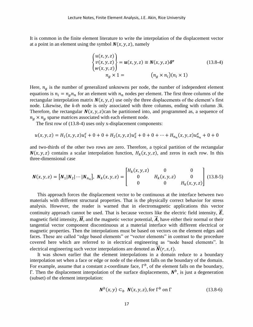
It is common in the finite element literature to write the interpolation of the displacement vector

at a point in an element using the symbol 𝑵(𝑥, 𝑦, 𝑧), namely

{

𝑢(𝑥, 𝑦, 𝑧)𝑣(𝑥, 𝑦, 𝑧)𝑤(𝑥, 𝑦, 𝑧)

} = 𝒖(𝑥, 𝑦, 𝑧) ≡ 𝑵(𝑥, 𝑦, 𝑧)𝜹𝒆 (13.8-4)

𝑛𝑔 × 1 = (𝑛𝑔 × 𝑛𝑖)(𝑛𝑖 × 1)

Here, 𝑛𝑔 is the number of generalized unknowns per node, the number of independent element

equations is 𝑛𝑖 = 𝑛𝑔𝑛𝑛 for an element with 𝑛𝑛 nodes per element. The first three columns of the

rectangular interpolation matrix 𝑵(𝑥, 𝑦, 𝑧) use only the three displacements of the element’s first

node. Likewise, the k-th node is only associated with three columns, ending with column 3k.

Therefore, the rectangular 𝑵(𝑥, 𝑦, 𝑧)can be partitioned into, and programmed as, a sequence of

𝑛𝑔 × 𝑛𝑔 sparse matrices associated with each element node.

The first row of (13.8-4) uses only x-displacement components:

𝑢(𝑥, 𝑦, 𝑧) = 𝐻1(𝑥, 𝑦, 𝑧)𝑢1𝑒 + 0 + 0 + 𝐻2(𝑥, 𝑦, 𝑧)𝑢2

𝑒 + 0 + 0 +⋯+𝐻𝑛𝑛(𝑥, 𝑦, 𝑧)𝑢𝑛𝑛𝑒 + 0 + 0

and two-thirds of the other two rows are zero. Therefore, a typical partition of the rectangular

𝑵(𝑥, 𝑦, 𝑧) contains a scalar interpolation function, 𝐻𝑘(𝑥, 𝑦, 𝑧), and zeros in each row. In this

three-dimensional case

𝑵(𝑥, 𝑦, 𝑧) = [𝑵1|𝑵2|⋯ |𝑵𝑛𝑛], 𝑵𝑘(𝑥, 𝑦, 𝑧) = [

𝐻𝑘(𝑥, 𝑦, 𝑧) 0 0

0 𝐻𝑘(𝑥, 𝑦, 𝑧) 0

0 0 𝐻𝑘(𝑥, 𝑦, 𝑧)] (13.8-5)

This approach forces the displacement vector to be continuous at the interface between two

materials with different structural properties. That is the physically correct behavior for stress

analysis. However, the reader is warned that in electromagnetic applications this vector

continuity approach cannot be used. That is because vectors like the electric field intensity, �⃗⃗� ,

magnetic field intensity, �⃗⃗⃗� , and the magnetic vector potential, �⃗⃗� , have either their normal or their

tangential vector component discontinuous at a material interface with different electrical or

magnetic properties. Then the interpolations must be based on vectors on the element edges and

faces. These are called “edge based elements” or “vector elements” in contrast to the procedure

covered here which are referred to in electrical engineering as “node based elements”. In

electrical engineering such vector interpolations are denoted as �⃗⃗� (𝑟, 𝑠, 𝑡). It was shown earlier that the element interpolations in a domain reduce to a boundary

interpolation set when a face or edge or node of the element falls on the boundary of the domain.

For example, assume that a constant z-coordinate face, Γ𝑏, of the element falls on the boundary,

Γ. Then the displacement interpolation of the surface displacements, 𝑵𝑏, is just a degeneration

(subset) of the element interpolation:

𝑵𝑏(𝑥, 𝑦) ⊂𝑏 𝑵(𝑥, 𝑦, 𝑧), for Γ𝑏 on Γ (13.8-6)


18

13.9 Mechanical work in matrix form: Having converted the displacements into matrix

forms in (13.8-4) and (13.8-6), the mechanical work definition of (13.3-3) can now be written in

terms of the element displacement degrees of freedom, and thereby define element and system

load vectors. Begin with the mechanical work definition for any elastic system:

𝑊 = ∫𝜹𝑇𝒇 𝑑𝑉

𝑉

+∫𝜹𝑇𝑻 𝑑𝑆

𝑆

+∑ 𝜹𝑘𝑇𝑭𝑘

𝑘=𝑛𝑃

𝑘=1

The external point load work summation can be replaced as with a scalar product of the system

displacements, 𝜹, and a system point load vector, 𝑭, that is zero except where point loads are

input at a node:

∑ 𝜹𝑘𝑇𝑭𝑘

𝑘=𝑛𝑃𝑘=1 = 𝜹𝑇𝑭 = 𝑭𝑇𝜹 (13.9-1)

Having divided the elastic domain and its surface with a mesh the volume integral of any

quantity becomes the sum of the integrals of that quantity in the element:

∫___𝑑𝑉

𝑉

=∑ ∫ ___𝑑𝑉

𝑉𝑒

𝑛𝑒

𝑒=1

Therefore, the work done by body forces becomes

∫𝜹𝑇𝒇 𝑑𝑉

𝑉

=∑ ∫ (𝑵(𝑥, 𝑦, 𝑧)𝜹𝒆)𝑇𝒇 (𝑥, 𝑦, 𝑧)𝑑𝑉

𝑉𝑒

𝑛𝑒

𝑒=1

=∑ 𝜹𝒆𝑇∫ 𝑵𝑇(𝑥, 𝑦, 𝑧)𝒇 (𝑥, 𝑦, 𝑧)𝑑𝑉

𝑉𝑒

𝑛𝑒

𝑒=1≡∑ 𝜹𝒆𝑇

𝑛𝑒

𝑒=1𝒄𝑓𝑒

(1 × 𝑛𝑖)(𝑛𝑖 × 𝑛𝑔)(𝑛𝑔 × 1), and here 𝑛𝑔 = 𝑛𝑠

This defines the resultant element nodal load resultants due to body forces:

𝒄𝑓𝑒 ≡ ∫ 𝑵𝑇(𝑥, 𝑦, 𝑧)𝒇 (𝑥, 𝑦, 𝑧)𝑑𝑉

𝑉𝑒. (13.9-2)

(𝑛𝑖 × 1) = (𝑛𝑖 × 𝑛𝑔)(𝑛𝑔 × 1)

The remaining contribution to the external work due to surface tractions, ∫ 𝜹𝑇𝑻 𝑑𝑆

𝑆, is also split

by the mesh generation to the sum over the boundary segments having a non-zero traction:

∫𝜹𝑇𝑻 𝑑𝑆

𝑆

=∑ ∫ (𝑵𝒃(𝑥, 𝑦)𝜹𝒃)𝑇𝑻 (𝑥, 𝑦)𝑑𝑆

Γ𝑏

𝑛𝑏

𝑏=1

=∑ 𝜹𝒃𝑇∫ 𝑵𝒃

𝑇(𝑥, 𝑦)𝑻 (𝑥, 𝑦 )𝑑𝑆

Γ𝑏

𝑛𝑏

𝑏=1≡∑ 𝜹𝒃

𝑇𝑛𝑏

𝑏=1𝒄𝑇𝑏

This defines the resultant boundary segment nodal load resultants due to tractions:


19

𝒄𝑇𝑏 ≡ ∫ 𝑵𝒃

𝑇(𝑥, 𝑦)𝑻(𝑥, 𝑦)𝑑𝑆

Γ𝑏. (13.9-3)

(𝑛𝑔𝑛𝑛𝑏 × 1) = (𝑛𝑔𝑛𝑛𝑏 × 𝑛𝑔)(𝑛𝑔 × 1)

where 𝑛𝑏 is the number of boundary segments and 1 ≤ 𝑛𝑛𝑏 ≤ 𝑛𝑛 is the number of nodes on the

segment.

When each set of element displacements, 𝜹𝒆, are identified, using the element node

connection list, with their positions in the system displacement vector, 𝜹, then scattering all of

the body force node resultants gives the assembled system level body force resultant:

∑ 𝜹𝒆𝑇𝑛𝑒𝑒=1 𝒄𝑓

𝑒 = 𝜹𝑇𝒄𝑓

When each set of boundary displacements, 𝜹𝒃, are identified, using the boundary node

connection list, with their positions in the system displacement vector, 𝜹, then scattering all of

the surface traction node resultants gives the assembled system level traction resultant:

∑ 𝜹𝑏𝑇𝑛𝑏

𝑏=1 𝒄𝑇𝑏 = 𝜹𝑇𝒄𝑇,

Some authors like to introduce an ‘assembly symbol’, 𝒜, to emphasize that the system level

body force resultant, 𝒄𝑓, is the assembly (scattering) of all of the element level body force

resultants, 𝒄𝑓𝑒, and that the system level surface traction resultant, 𝒄𝑇, is the assembly (scattering)

of all of the boundary segment level traction resultants, 𝒄𝑇𝑏 :

𝒄𝑓 = 𝒜𝑒 𝒄𝑓𝑒 and 𝒄𝑇 = 𝒜𝑏 𝒄𝑇

𝑏 (13.9-4)

(𝑛𝑔𝑛𝑚 × 1) ⇐+ (𝑛𝑖 × 1) (𝑛𝑔𝑛𝑚 × 1) ⇐+ (𝑛𝑖 × 1)

Here, the number of system equations is 𝑛𝑑 = 𝑛𝑔𝑛𝑚, for a mesh with 𝑛𝑚 nodes. Finally, the

external work is found to be the scalar product of the system displacement vector and a set of

assembled force vectors:

𝑊 = 𝜹𝑇𝒄𝑓 + 𝜹𝑇𝒄𝑇 + 𝜹

𝑇𝑭 ≡ 𝜹𝑇𝒄 (13.9-5)

where 𝒄 denotes the system resultant force vector, to which the initial strain forces will be added.

13.10 The Strain-Displacement Matrix: Next the six strains within an element, 𝜺, also

need to be defined in terms of the element displacements, 𝜹𝒆. This leads to a larger rectangular

matrix, usually denoted in the finite element literature as 𝑩𝒆(𝑥, 𝑦, 𝑧), which is known as the

strain-displacement matrix. It has six rows and 𝑛𝑖 = 𝑛𝑛𝑛𝑔 columns that correspond to the

element displacements. Recall that each component can be interpolated using the scalar forms in

(13.8-1). From the geometric definitions of section 13.4 the six strain components are

휀𝑥 =𝜕𝑢

𝜕𝑥=

𝜕𝑯(𝑥,𝑦,𝑧)

𝜕𝑥 𝒖𝒆, 휀𝑦 =

𝜕𝑣

𝜕𝑦=


𝜕𝑦 𝒗𝒆, 휀𝑧 =

𝜕𝑤

𝜕𝑧=


𝜕𝑧 𝒘𝒆,

𝛾𝑥𝑦 =𝜕𝑢

𝜕𝑦+

𝜕𝑣

𝜕𝑥=


𝜕𝑦 𝒖𝒆 +


𝜕𝑥 𝒗𝒆,


20

𝛾𝑥𝑧 =𝜕𝑢

𝜕𝑧+𝜕𝑤

𝜕𝑥=


𝜕𝑧 𝒖𝒆 +


𝜕𝑥 𝒘𝒆,

𝛾𝑦𝑧 =𝜕𝑣

𝜕𝑧+𝜕𝑤

𝜕𝑦=


𝜕𝑧 𝒗𝒆 +


𝜕𝑦 𝒘𝒆.

These can be re-arranged into the matrix format

{


𝑒

= 𝜺𝒆 = 𝑩𝒆(𝑥, 𝑦, 𝑧) 𝜹𝒆 (13.10-1)

(𝑛𝑟 × 1) = (𝑛𝑟 × 𝑛𝑖)(𝑛𝑖 × 1)

The first row has triplet entries of

휀𝑥 =𝜕𝐻1𝜕𝑥

𝑢1𝑒 + 0 + 0 +

𝜕𝐻2𝜕𝑥

𝑢2𝑒 + 0 + 0 +⋯+

𝜕𝐻𝑛𝑛𝜕𝑥

𝑢𝑛𝑛𝑒 + 0 + 0

and the last row has triplet entries of

𝛾𝑦𝑧 = 0 +𝜕𝐻1𝜕𝑧

𝑣1𝑒 +

𝜕𝐻1𝜕𝑦

𝑤1𝑒 +⋯+ 0 +

𝜕𝐻1𝜕𝑧

𝑣𝑛𝑛𝑒 +

𝜕𝐻1𝜕𝑦

𝑤𝑛𝑛𝑒

Like the vector interpolations, the rectangular 𝑩𝒆 strain-displacement matrix can be partitioned

into, and programmed as, rectangular nodal contributions 𝑩𝒆(𝑥, 𝑦, 𝑧) = [𝑩𝒆1|𝑩𝒆2|⋯ |𝑩

𝒆𝑛𝑛],

with a typical classic definition partition (with 𝑛𝑟 = 6 rows of strains and 𝑛𝑔 = 3 displacement

component columns) being

𝑩𝒆𝑘 =

[ 𝐻𝑘,𝑥 0 0

0 𝐻𝑘,𝑦 0

0 0 𝐻𝑘,𝑧 𝐻𝑘,𝑦 𝐻𝑘,𝑥 0

𝐻𝑘,𝑧 0 𝐻𝑘,𝑥 0 𝐻𝑘,𝑧 𝐻𝑘,𝑦]

, 𝐻𝑘,𝑥 = 𝜕𝐻𝑘 𝜕𝑥⁄ ,𝐻𝑘,𝑦 = 𝜕𝐻𝑘 𝜕𝑦⁄ (13.10-2)

(𝑛𝑟 × 𝑛𝑔)

In the software provided, the strains (and stresses) are ordered as in Fig. 13.4-2. The

algorithm for filling the full 𝑩𝒆 matrix for plane-stress or plane-strain applications is shown in

B_planar_elastic.m in Fig. 13.10-1. The axisymmetric stress version adds one additional row to

the definition, as shown in B_axisym_elastic.m in Fig. 13.10-2. All five options for the strain-

displacement choices listed in Fig. 13.4-2 are included in the single script B_matrix_elastic.m in

the functions library.


21

Figure 13.10-1 Strain-displacement matrix for plane-stress or -strain

Figure 13.10-2 Strain-displacement matrix for axisymmetric stress model


22

13.11 Stiffness matrix: The strain energy of (13.5-1) defines the stiffness matrix of an

elastic system by relating its integrand to the unknown displacements:

𝑈 =1

2∫𝝈𝑇𝜺 𝑑𝑉

𝑉

=1

2∑ ∫ 𝝈𝒆𝑇𝜺𝑒𝑑𝑉

𝑉𝑒

𝑛𝑒

𝑒=1=1

2∑ ∫ (𝑬𝒆𝜺𝑒)𝑇𝜺𝑒𝑑𝑉

𝑉𝑒

𝑛𝑒

𝑒=1

=1

2∑ ∫ 𝜺𝑒𝑇𝑬𝒆𝑇𝜺𝑒𝑑𝑉

𝑉𝑒

𝑛𝑒

𝑒=1=1

2∑ ∫ (𝑩𝒆𝜹𝒆)𝑇𝑬𝒆(𝑩𝒆𝜹𝒆)𝑑𝑉

𝑉𝑒

𝑛𝑒

𝑒=1

=1

2∑ 𝜹𝒆 𝑇 [∫ 𝑩𝑒𝑇𝑬𝒆 𝑩𝑒𝑑𝑉

𝑉𝑒]

𝑛𝑒

𝑒=1𝜹𝒆 =

1

2∑ 𝜹𝒆 𝑇[𝑺𝑒]

𝑛𝑒

𝑒=1𝜹𝒆

So that the element stiffness matrix is defined as

𝑺𝑒 = ∫ 𝑩𝑒𝑇𝑬𝒆 𝑩𝑒𝑑𝑉

𝑉𝑒 (13.11-1)

(𝑛𝑖 × 𝑛𝑖) = (𝑛𝑖 × 𝑛𝑟)(𝑛𝑟 × 𝑛𝑟)(𝑛𝑟 × 𝑛𝑖)

For two-dimensional problems the differential volume is 𝑑𝑉 = ∫ 𝑡𝑒(𝑥, 𝑦) 𝑑𝐴

𝐴𝑒 where 𝑡𝑒 is

the local thickness of the planar section, 𝐴𝑒. Usually, the thickness is constant in each element. If

the thickness is the same constant in all elements, and there are no external point loads, then it

cancels out since it appears in every integral. Many commercial finite element systems, and the

application scripts supplied here, allow the plane-stress elements to have different thicknesses.

When the elements do not have the same constant thickness the analysis is called a 2.5D

analysis. It approximates a 3D part and can be used in a preliminary analysis to guide the local

mesh control needed in the actual 3D study. Alternately, it can be considered as a useful

validation check of a prior 3D analysis.

Usually, the stresses in a 2.5D model are accurate except in the immediate region adjacent to

changes in the element thicknesses. If the thickness is to be allowed to continuously vary then it

is usually input at the element nodes and interpolated to give the local thickness, 𝑡𝑒(𝑥, 𝑦). A

variable thickness element clearly requires the stiffness matrix to be evaluated by numerical

integration with an appropriately higher number of integration points. If the thickness is

continuously varying then it can be input as an additional fake coordinate and is simple to gather

to the nodes of each element for interpolation.

13.12 Work done by initial strains: When any initial strain is present its name implies

the fact that it is constant from the beginning of an imposed mechanical strain (and stress) to the

end of that strain. Therefore, the work that it does differs from (13.5-1) by a factor of two and is

𝑊0 = ∫ 𝝈𝑇𝜺𝟎 𝑑𝑉

𝑉 (13.12-1)

𝑊0 = ∫𝝈𝑇𝜺𝟎 𝑑𝑉

𝑉

=∑ ∫ 𝝈𝒆𝑇𝜺𝟎𝑒𝑑𝑉

𝑉𝑒

𝑛𝑒

𝑒=1=∑ ∫ (𝑩𝒆𝜹𝒆)𝑇𝑬𝒆𝜺𝟎

𝑒𝑑𝑉

𝑉𝑒

𝑛𝑒

𝑒=1

This defines the element initial strain resultant force vector as


23

𝑊0 = ∑ 𝜹𝒆𝑇𝑛𝑒𝑒=1 𝒄0

𝑒 with 𝒄𝟎𝒆 = ∫ 𝑩𝑒𝑇𝑬𝒆𝜺𝟎

𝑒𝑑𝑉

𝑉𝑒 (13.12-2)

(𝑛𝑖 × 1) = (𝑛𝑖 × 𝑛𝑟)(𝑛𝑟 × 𝑛𝑟)(𝑛𝑟 × 1)

13.13 Matrix equilibrium equations: Having converted all of the work and strain energy

contributions in their interpolated matric forms the matrix equations of equilibrium are:

𝑺 𝜹 = 𝒄𝟎 + 𝒄𝑷 + 𝒄𝑻 + 𝒄𝒇 + 𝒄𝑵𝑩𝑪 ≡ 𝒄 (13.13-1)

Here, all of the element and boundary contributions are assembled into the large system matrices

by direct scattering of the rows and columns, or (in theory) by the direct Boolean algebra:

𝑺 = ∑ 𝜷𝑒𝑇[𝑺𝑒]

𝑛𝑒𝑒=1 𝜷𝒆,

𝒄𝒇 =∑ 𝜷𝑒𝑇𝑛𝑒

𝑒=1𝒄𝒇𝒆, 𝒄𝑻 =∑ 𝜷𝑏

𝑇𝑛𝑏

𝑏=1𝒄𝑻,𝒃 𝒄𝟎 =∑ 𝜷𝑒𝑇

𝑛𝑒

𝑒=1𝒄𝟎𝒆

13.14 Plane stress analysis: For plane-stress and plane-strain the order of the strain

components and the Strain-Displacement relations, 𝜺𝒆 = 𝑩𝒆𝜹𝒆, are:

𝜺𝒆 = {

휀𝑥휀𝑦𝛾𝑥𝑦}

𝑒

, 𝑩𝒆 = [ 𝑩𝒆1 𝑩𝒆2 ⋯ 𝑩𝒆𝑘 ⋯ 𝑩𝒆𝑛𝑛], 𝑩𝒆𝑘 = [

𝐻𝑘,𝑥 0

0 𝐻𝑘,𝑦 𝐻𝑘,𝑦 𝐻𝑘,𝑥

]

3 × 1 3 × ( 𝑛𝑔 ∗ 𝑛𝑛) 3 × (𝑛𝑔 = 2)

𝜹𝒆𝑇 = [𝑢1, 𝑣1, 𝑢2, ⋯ , 𝑣𝑘, ⋯ , 𝑢𝑛𝑛 , 𝑣𝑛𝑛]𝑒

1 × (𝑛𝑔 ∗ 𝑛𝑛)

The plane-stress stress components order and their relation to the material constitutive law

(Hooke’s Law) is

{


} =𝐸

1−𝜐2[1 𝜐 0𝜐 1 00 0 (1 − 𝜐) 2⁄

] {


𝐸𝛼∆𝑇

1−𝜐{110}

where 𝐸 is the elastic modulus (Young’s modulus),𝜐 is Poisson’s ratio, 𝛼 is the coefficient of

thermal expansion (CTE), and ∆𝑇 is the increase in temperature from the stress free state at the

point where the stress is evaluated.

The element stiffness matrix for a domain of thickness 𝑡𝑒 is

𝑺𝑒 = ∫ 𝑩𝑒𝑇𝑬𝒆 𝑩𝑒 𝑡𝑒𝑑𝐴 = ∑ 𝑩𝒆𝑞𝑇 𝑬𝑞

𝑒𝑩 𝑞 𝑒 𝑡𝑞

𝑒|𝑱𝑞𝑒 |

𝑛𝑞𝑞=1

𝐴𝑒𝑤𝑞.

The resultant body force vector and edge traction vector are

𝒄𝒇𝒆 = ∫ 𝑵𝒆𝑇𝒇 𝑡𝑒𝑑𝐴

𝐴𝑒= ∫ 𝑵𝒆𝑇{𝑵𝒆𝒇𝒆} 𝑡𝑒𝑑𝐴

𝐴𝑒=∑ 𝑵𝒆𝑞

𝑇{ 𝑵𝑞𝑒 𝒇𝑞

𝑒} 𝑡𝑞𝑒 |𝑱𝑞

𝑒 |𝑤𝑞𝑛𝑞

𝑞=1


24

𝒄𝑻𝒃 = ∫ 𝑵𝒃

𝑇𝑻 𝑡𝑏𝑑Γ

Γ𝑒= ∫ 𝑵𝒃

𝑇{𝑵𝒃𝑻𝒃} 𝑡𝑏𝑑Γ

Γ𝑒= ∑ 𝑵𝒃𝑞

𝑇 { 𝑵𝑞

𝑏 𝑻𝑞𝑏} 𝑡𝑞

𝑏 |𝑱𝑞𝑏|𝑤𝑞

𝑛𝑞𝑞=1 ,

respectively, and the thermal strain loading resultant is

𝒄𝜶𝒆 = ∫ 𝑩𝑒𝑇𝑬𝒆𝜺0

𝑒 𝑡𝑒𝑑𝐴

𝐴𝑒= ∫ 𝑩𝑒𝑇𝑬𝒆𝛼𝑒∆𝑇 {

110} 𝑡𝑒𝑑𝐴

𝐴𝑒=∑ 𝑩𝒆𝑞

𝑇 𝑬𝑞𝑒 𝛼𝑞

𝑒 {𝑯𝑞𝑒 ∆𝑇𝑞

𝑒} {110} 𝑡𝑞

𝑒|𝑱𝑞𝑒 |

𝑛𝑞

𝑞=1

if the scalar temperature changes at the nodes are interpolated with 𝑯 𝑒 .

For the common three node “constant stress triangle” the Strain-Displacement matrix is

𝑩𝒆 =1

2𝐴𝑒[

𝑏1 0 𝑏2 0 𝑏3 00 𝑐1 0 𝑐2 0 𝑐3 𝑐1 𝑏1 𝑐2 𝑏2 𝑐3 𝑏3

],

the resultant body force vector for constant 𝑓𝑥 and 𝑓𝑦 values is

𝒄𝒇𝒆 = 𝑡𝑒𝐴𝑒[𝑓𝑥 𝑓𝑦 𝑓𝑥 𝑓𝑦 𝑓𝑥 𝑓𝑦]𝑇/3

and the resultant edge traction force vector for constant 𝑇𝑥 and 𝑇𝑦 values is

𝒄𝑻𝒃 = 𝑡𝑒𝐿𝑒[𝑇𝑥 𝑇𝑦 𝑇𝑥 𝑇𝑦]

𝑇/2.

13.15 Axisymmetric stress analysis: In axisymmetric stress analysis a planar area is

revolved about an axis lying outside the area. The analysis is similar to the plane-stress analysis

except of three facts. First, at any point in the area the thickness is proportional to the radial

position, 𝑡𝑒 = 2𝜋 R(r, s). Secondly, at any point there is now a complete hoop of material

around the axis. Any displacement parallel to the axis does not change the length of that

filament of material; but any displacement in the radial direction, 𝑢(𝑟, 𝑠), changes the

circumferential length from 2𝜋 R to 2𝜋 (R + u). Thirdly, such a deformation means that there

exists a third normal stress, 𝜎𝜃𝜃 ⟺ 𝜎𝑧𝑧 called the hoop stress, due to the additional hoop strain

휀𝑧𝑧 ⟺ 휀𝜃𝜃 =∆𝐿

𝐿=

2𝜋 (R+u)−2𝜋 R

2𝜋 R=

u(r,s)

R(r,s)=

𝐇(r,s)𝒖𝒆

R(r,s).

Thus, the plane-stress or plane-strain ordering of the strain components is increased by

adding a fourth row, which means that the strain-displacement matrix also has a new fourth row

dependent only on u:

{

휀𝑅휀𝑦𝛾𝑅𝑦휀𝜃

}

𝑒

, 𝑩𝒆𝑘 = [

𝐻𝑘,𝑥0

𝐻𝑘,𝑦𝐻𝑘 𝑅⁄

0𝐻𝑘,𝑦𝐻𝑘,𝑥0

]

This is the first strain component defined by a displacement value instead of the gradient of that

displacement. There are many solids of revolution that touch the axis of revolution (R ≡ 0)


25

where, by inspection, u ≡ 0 and the hoop strain takes an indeterminate form of 0/0. Taking

additional derivatives shows that 휀𝜃𝜃 = 0 as 𝑅 → 0. This common occurrence is important in

finite element analysis when numerical integration is used to evaluate the stiffness matrix of

triangular elements. Some of the integration rules for triangles have quadrature points at the

midpoint of the edges of the triangle. If an edge of any triangle falls on the axis of revolution,

which is common, such an integration rule would cause division by zero and abort the program.

The fix is simple; just pick a rule without points on the edge of the triangle to avoid division by

zero.

Of course, the presence of the hoop strain means that there is a third normal stress, 𝜎𝜃, which

must be included in the stress vector and which must be related to the material properties:

{

𝜎𝑅𝜎𝑧𝜏𝑟𝑧𝜎𝜃

} =𝐸

(1+𝜐)(1−2𝜐)[

𝑎 𝜈𝜈 𝑎

0 𝜈0 𝜈

0 0𝜈 𝜈

𝑏 00 𝑎

] {

휀𝑅휀𝑧𝛾𝑟𝑧휀𝜃


(1−2𝜐){

1101

}.

𝑎 = (1 − 𝜐), 𝑏 = (1 − 2𝜐)/2, 𝜐 ≠ 0.5

13.16 Solid stress analysis: All of the finite element stress analysis programs are

essentially the same except for minor differences in the post-processing. The majority of any

applications system consists of reading and checking the data, creating and assembling

application dependent elements, enforcing the essential boundary conditions, solving the

equilibrium equations, displaying and saving the generalized displacements, and completing any

application dependent post-processing of the elements. Note that mainly the generation and post-

processing of the application dependent elements is what changes. The other 95% of the coding

is unchanged. There may be additional calculations for an error estimator, but they are not

required. Also, there are usually several off-line features such as resources to graphically display

the results of importance.

All of the planar problems discussed above are easily extended to three-dimensions, and the

supplied Matlab scripts will execute such problems just by changing the number of physical

space dimensions to three (𝑛𝑠=3), utilizing the eight node hexahedral (brick) element by setting

the parametric element space to three and the number of nodes to eight (𝑛𝑝=3, 𝑛𝑛=8), and

selecting the correct number of integration points, which is usually 23=8 but may be 27. The size

of the constitutive matrix, 𝑬𝒆, and the operator matrix, 𝑩𝒆, must be increased to six (𝑛𝑟=6) by

adding three more strain displacement relations. Of course, additional elements can be added to

the element library. However, most three-dimension problems are better solved with commercial

software simply because they have automatic solid element mesh generators and offer several

good graphical post-processing tools.

To illustrate those points again the discussion of three-dimensional solid stress analysis will

be limited to one of the simplest implementations. The linear four-node tetrahedra element (here

called the pyramid P4 to avoid confusion with triangular element shorthand) was the first solid

element. It is relatively easy to create them with an automatic mesh generator. But is gives only

constant stresses within its volume and is no longer recommended unless a very large number of

them are used (compared to the number of higher order elements they replace). The ten-node

tetrahedra (P10) are commonly used since they can be obtained from the same automatic mesh

generators as the P4 elements. However, they are only interpolating the displacements with

complete quadratics, and thus give only linearly changing stress estimates.


26

The hexahedra element family is considered to be a better choice for solid stress analysis

because they have higher order interior interpolation functions than do the tetrahedral elements

having the same number of edge nodes. They are more difficult to create with an automatic mesh

generator and that restricts they widespread use. The eight-node element (H8) is used here and is

validated by running a three-dimensional patch test.

13.17 Material failure criteria: The main purpose of a stress analysis, after understanding

the response of the structure, is to determine if any material point in the domain has failed. That

means that one of the many potential failure criteria must be selected and compared to one or

more experimentally measured material stress limits. The three most common measurements are

the failure stress in tension, 𝑘𝑡, also called the yield stress, the absolute value of the failure stress

in compression, 𝑘𝑐 , and the absolute value of the failure stress in pure shear, 𝑘𝑠. The tension

limit, 𝑘𝑡, is the most commonly used comparison value. Most tabulations of material stress limits

give only the tension limit, 𝑘𝑡, a few tables also give the compression limit, 𝑘𝑐, of a material. It is

rare to find measured shear stress limits published, but they can be theoretically related to the

tension limit.

These material stress limits can also be related to failure criterion based on energy portions

stored in the material. At the elastic limit the strain energy is the sum of the elastic energy of

distortion (which defines the von Mises criterion 𝜎𝑀) and the elastic energy of the volume

change (which defines the Burzynski criterion 𝜎𝐵).

A contour plot of a stress component or failure criteria can give an engineer a general

understanding the response of the structure. However, a non-dimensional plot of the stress or

failure criteria divided by the measured stress limit(s) indicates the regions of likely material

failure. There, a ratio value of unity indicates impending failure, a value greater than one shows a

region of failure, while a value less than one is still a safe region. Some commercial codes label

such plots as a factor of safety plot which is misleading because the true Factor of Safety

depends of several other considerations. Here such plots are called ‘failure scale’ plots.

Finite element formulations often use the Voigt stress notation as a condensed form of the

stress tensor [𝝈]:

𝝈𝑇 = [𝜎𝑥 𝜎𝑦 𝜎𝑧 𝜏𝑥𝑦 𝜏𝑥𝑧 𝜏𝑦𝑧] ⇔ [𝝈] = [

𝜎𝑥𝑥 𝜏𝑥𝑦 𝜏𝑥𝑧𝜏𝑥𝑦 𝜎𝑦𝑦 𝜏𝑦𝑧𝜏𝑥𝑧 𝜏𝑦𝑧 𝜎𝑧𝑧

] (13.17-1)

At any point in a stressed solid there are three mutually orthogonal planes where the shear

stresses vanish and only the three normal stresses remain. Those three normal stresses are called

the principal stresses (𝜎1, 𝜎2, 𝜎3, also denoted as 𝑃1, 𝑃2, 𝑃3). The principal stresses are utilized to

define the most common failure criteria theories for most materials. Therefore, their calculation

is usually obtained at each quadrature point in a stress analysis. The principal stresses are found

from a small 3 × 3 classic eigen-problem:

|[𝝈] − 𝜆𝑘[𝑰]| = 0, 𝑘 = 1,2, 3 (13.17-2)

where [𝑰] is the identity matrix, [𝝈] is the 3 × 3 symmetric second order stress tensor, 𝜆𝑘, is a

real principal stress value giving the algebraic maximum stress, 𝜆1 = 𝜎1, the intermediate stress

𝜆2 = 𝜎2, and the minimum stress 𝜆3 = 𝜎3. (This process is valid for finding the principle values

and directions for any other second order symmetric tensor, such as the moment of inertia


27

tensor.) The principle stresses are obtained from the Matlab function eig (in reverse order), with

only [𝝈] as the single argument.

If tension occurs at the point then 𝜎1 gives the value of the maximum tension. Likewise, if

compression occurs at the point 𝜎3 gives the value of the maximum compression stress. A state

of plane-stress gives 𝜎2 = 0. The shear ‘stress intensity’ is defined as 𝜎𝐼 = 𝜎1 − 𝜎3 = 2𝜏𝑚𝑎𝑥

where 𝜏𝑚𝑎𝑥 is the absolute maximum shear stress on any plane in the solid at that point. For

plane-stress problems it is common (in mechanics) to find the maximum in-plane shear stress

from

𝜏𝑝𝑙𝑎𝑛𝑒 = √(𝜎𝑥−𝜎𝑦)2

2

+ 𝜏𝑥𝑦2 ≤ 𝜏𝑚𝑎𝑥 =1

2(𝜎1 − 𝜎3) (13.17-3)

But, if the thickness of the planar part is not very small the absolute maximum shear stress can

lie in a different plane and has to be found from the above three-dimensional calculation.

The principal stresses define other physically important quantities, including the hydrostatic

pressure 𝑝 = (𝜎1 + 𝜎2 + 𝜎3)/3 which represents a uniform normal stress in all directions, the

deviatoric stresses, [�̂�] ≡ [𝝈] − 𝑝[𝑰], the distortional energy, and the volume change (deviatoric)

energy.

Most commercial finite element programs display the von Mises criterion (also known as the

Effective Stress criterion) as the default stress plot. However, it is the valid criteria only when

the material is ductile and when the measured failure stresses in tension and compression are

equal, 𝑘𝑡 = 𝑘𝑐. The latter restriction is only valid for a few materials.

The von Mises criterion actually calculates the distortional energy at a point which is

proportional to the square root of the sum of the squares of the differences in the principle

stresses. The von Mises ‘stress’ is defined in terms of the principle stresses or stress components

as

𝜎𝑀 =1

√2√(𝜎1 − 𝜎2)2 + (𝜎1 − 𝜎3)2 + (𝜎2 − 𝜎3)2 (13.17-4)

𝜎𝑀 =1

√2√(𝜎𝑦𝑦 − 𝜎𝑥𝑥)

2+ (𝜎𝑧𝑧 − 𝜎𝑥𝑥)2 + (𝜎𝑧𝑧 − 𝜎𝑦𝑦)

2+ 6(𝜏𝑥𝑦2 + 𝜏𝑥𝑧2 + 𝜏𝑦𝑧2) (13.17-5)

which has the units of stress, but is not a physical stress. That measure is called the Equivalent

stress or the Von Mises stress. For a ductile material, its tension stress limit (yield stress), 𝑘𝑡, is

compared to the 𝜎𝑀 value to see if material has failed based on its distortional energy at the

point. Material failure is declared when 𝜎𝑀 ≥ 𝑘𝑡, or when the ‘failure scale’ 𝜎𝑀 𝑘𝑡⁄ > 1. That is

checked because in a uniaxial tension test of material failure the distortional energy measure

reduces to

𝜎𝑀 =1

√2√(𝑘𝑡 − 0)2 + (𝑘𝑡 − 0)2 + (0 − 0)2 =

√2

√2𝑘𝑡 = 𝑘𝑡.

For a state of plane-stress (𝜎2 = 0) the von Mises distortional energy measure yield curve plots

as an ellipse in the principle stress space. Points inside the ellipse have not failed, points on the

ellipse (yield curve) are impending to fail, and any stress points outside the ellipse denote failed

material points. The von Mises ellipse is centered at the origin and is symmetric about the 45° angle.

The Burzynski failure criterion states that a material fails when the volume change

(deviatoric) energy at a point equals the deviatoric energy in a tension test at the limit of elastic


28

behavior. The Burzynski criteria requires that the failure stress in tension be different from that

in compression, 𝑘𝑡 ≠ 𝑘𝑐, and it can also include the shear failure value, 𝑘𝑠. The ratio of the

tension to compression failures, 𝜅 ≡ 𝑘𝑐 𝑘𝑡⁄ , is often referred to as the ‘strength difference’. For a

state of plane-stress (𝜎2 = 0) the Burzynski deviatoric energy measure also plots as an ellipse in

the principle stress space. The Burzynski ellipse better fits failure data points than the von Mises

ellipse when 𝑘𝑡 ≠ 𝑘𝑐. In other words, for such materials the failure points, in the principle stress

space, fall on the Burzynski ellipse but fall inside the von Mises ellipse, or outside it, or both.

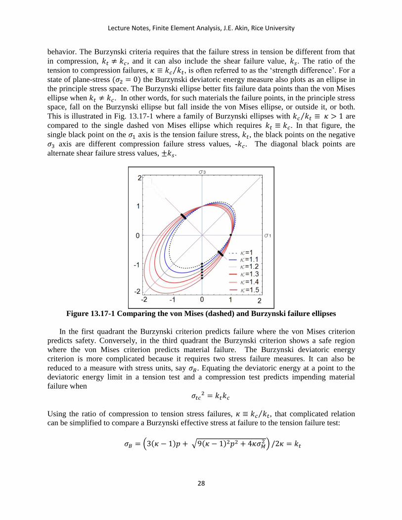
This is illustrated in Fig. 13.17-1 where a family of Burzynski ellipses with 𝑘𝑐 𝑘𝑡 ≡ 𝜅⁄ > 1 are

compared to the single dashed von Mises ellipse which requires 𝑘𝑡 ≡ 𝑘𝑐. In that figure, the

single black point on the 𝜎1 axis is the tension failure stress, 𝑘𝑡, the black points on the negative

𝜎3 axis are different compression failure stress values, -𝑘𝑐. The diagonal black points are

alternate shear failure stress values, ±𝑘𝑠.

Figure 13.17-1 Comparing the von Mises (dashed) and Burzynski failure ellipses

In the first quadrant the Burzynski criterion predicts failure where the von Mises criterion

predicts safety. Conversely, in the third quadrant the Burzynski criterion shows a safe region

where the von Mises criterion predicts material failure. The Burzynski deviatoric energy

criterion is more complicated because it requires two stress failure measures. It can also be

reduced to a measure with stress units, say 𝜎𝐵. Equating the deviatoric energy at a point to the

deviatoric energy limit in a tension test and a compression test predicts impending material

failure when

𝜎𝑡𝑐2 = 𝑘𝑡𝑘𝑐

Using the ratio of compression to tension stress failures, 𝜅 ≡ 𝑘𝑐 𝑘𝑡⁄ , that complicated relation

can be simplified to compare a Burzynski effective stress at failure to the tension failure test:

𝜎𝐵 = (3(𝜅 − 1)𝑝 + √9(𝜅 − 1)2𝑝2 + 4𝜅𝜎𝑀2 ) /2𝜅 = 𝑘𝑡


29

Note that when the material failure stress is the same in tension and compression then the

Burzynski criterion reduces to the von Mises criterion at impending failure:

𝜎𝐵(@𝜅 = 1) = 𝜎𝑀 = 𝑘𝑡

Figure 13.17-2 shows a Burzynski ellipse with black points representing the most common

failure stress tests of: pure tension, pure compression, pure shear, bi-axial tension, and bi-axial

compression.

Figure 13.17-2 Common failure stress states on a Burzynski ellipse

All of the commercial finite element software packages include the calculation of the von Mises

criterion, but as of 2018 none are known to offer the Burzynski criterion. Figure 13.17-3 gives a

Matlab script to calculate the ‘failure scales’ for xxx common failure criterion using the stress

vector at a point.

XXX

Figure 13.17-3 Computing failure scales at a point

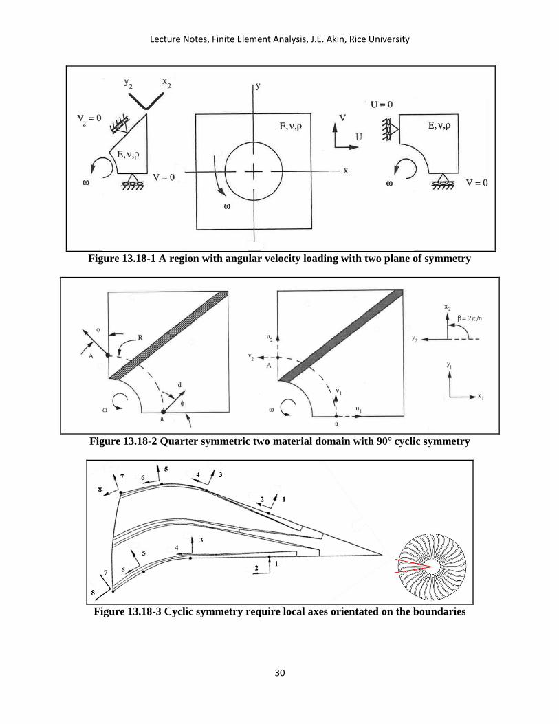
13.18 Symmetry and anti-symmetry: These topics were introduced earlier but they

become even more useful when dealing with solid parts that have planes of symmetry, anti-

symmetry, or cyclic symmetry. Figures 8.1-1 and 10.13-1 showed applications where one- and

two-dimensional symmetry conditions can occur for a scalar application. Based on operations

counts for solving linear systems, each symmetry, anti-symmetry, or cyclic symmetry plane used

in the model reduces the execution time by about a factor of eight. In other words, they speed up

the equation solution by a factor of 8𝑛, where n is the effective number of planes.


30

Figure 13.18-1 A region with angular velocity loading with two plane of symmetry

Figure 13.18-2 Quarter symmetric two material domain with 90° cyclic symmetry

Figure 13.18-3 Cyclic symmetry require local axes orientated on the boundaries


31

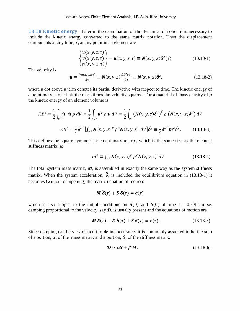
13.18 Kinetic energy: Later in the examination of the dynamics of solids it is necessary to

include the kinetic energy converted to the same matrix notation. Then the displacement

components at any time, 𝜏, at any point in an element are

{

𝑢(𝑥, 𝑦, 𝑧, 𝜏)𝑣(𝑥, 𝑦, 𝑧, 𝜏)𝑤(𝑥, 𝑦, 𝑧, 𝜏)

} = 𝒖(𝑥, 𝑦, 𝑧, 𝜏) ≡ 𝑵(𝑥, 𝑦, 𝑧)𝜹𝒆(𝜏). (13.18-1)

The velocity is

�̇� =𝜕𝒖(𝑥,𝑦,𝑧,𝜏)

𝜕𝜏≡ 𝑵(𝑥, 𝑦, 𝑧)

𝜕𝜹𝒆(𝜏)

𝜕𝜏≡ 𝑵(𝑥, 𝑦, 𝑧)𝜹�̇�, (13.18-2)

where a dot above a term denotes its partial derivative with respect to time. The kinetic energy of

a point mass is one-half the mass times the velocity squared. For a material of mass density of 𝜌

the kinetic energy of an element volume is

𝐾𝐸𝑒 =1

2∫ �̇� ∙

𝑉𝑒�̇� 𝜌 𝑑𝑉 =

1

2∫ �̇�𝑇

𝑉𝑒𝜌 �̇� 𝑑𝑉 =

1

2∫ (𝑵(𝑥, 𝑦, 𝑧)𝜹�̇�)

𝑇

𝑉𝑒𝜌 (𝑵(𝑥, 𝑦, 𝑧)𝜹�̇�) 𝑑𝑉

𝐾𝐸𝑒 =1

2𝜹�̇�

𝑇[∫ 𝑵(𝑥, 𝑦, 𝑧)𝑇 𝜌𝑒𝑵(𝑥, 𝑦, 𝑧)

𝑉𝑒 𝑑𝑉]𝜹�̇� ≡

1

2𝜹�̇�

𝑇𝒎𝒆𝜹�̇�. (13.18-3)

This defines the square symmetric element mass matrix, which is the same size as the element

stiffness matrix, as

𝒎𝒆 ≡ ∫ 𝑵(𝑥, 𝑦, 𝑧)𝑇 𝜌𝑒𝑵(𝑥, 𝑦, 𝑧)

𝑉𝑒 𝑑𝑉. (13.18-4)

The total system mass matrix, M, is assembled in exactly the same way as the system stiffness

matrix. When the system acceleration, �̈�, is included the equilibrium equation in (13.13-1) it

becomes (without dampening) the matrix equation of motion:

𝑴 �̈�(𝜏) + 𝑺 𝜹(𝜏) = 𝒄(𝜏)

which is also subject to the initial conditions on �̇�(0) and �̈�(0) at time 𝜏 = 0. Of course,

damping proportional to the velocity, say 𝓓, is usually present and the equations of motion are

𝑴 �̈�(𝜏) + 𝓓 �̇�(𝜏) + 𝑺 𝜹(𝜏) = 𝒄(𝜏). (13.18-5)

Since damping can be very difficult to define accurately it is commonly assumed to be the sum

of a portion, 𝛼, of the mass matrix and a portion, 𝛽, of the stiffness matrix:

𝓓 ≈ 𝛼𝑺 + 𝛽 𝑴. (13.18-6)


32

13.19 Summary

𝑛_𝑏 ⟷ 𝑛𝑏 ≡ Number of boundary segments

𝑛_𝑑 ⟷ 𝑛𝑑 ≡ Number of system unknowns = 𝑛_𝑔 × 𝑛_𝑚

𝑛_𝑒 ⟷ 𝑛𝑒 ≡ Number of elements

𝑛_𝑔 ⟷ 𝑛𝑔 ≡ Number of generalized DOF per node

𝑛_𝑖 ⟷ 𝑛𝑖 ≡ Number of unknowns per element = 𝑛_𝑔 × 𝑛_𝑛

𝑛_𝑚 ⟷ 𝑛𝑚 ≡ Number of mesh nodes

𝑛_𝑛 ⟷ 𝑛𝑛 ≡ Number of nodes per element or segment

𝑛_𝑃 ⟷ 𝑛𝑃 ≡ Number of point loads

𝑛_𝑝 ⟷ 𝑛𝑝 ≡ Dimension of parametric space

𝑛_𝑞 ⟷ 𝑛𝑞 ≡ Number of total quadrature points

𝑛_𝑟 ⟷ 𝑛𝑟 ≡ Number of rows in the 𝑩𝒆 matrix (and material matrix)

𝑛_𝑠 ⟷ 𝑛𝑠 ≡ Dimension of physical space

b = boundary segment number e = element number

⊂ = subset ∪ = union of sets

Boundary, element, and system unknowns: 𝜹𝒃 ⊂𝑏 𝜹𝒆 ⊂𝑒 𝜹

Geometry: Ω𝑒 ≡ Element domain Ω = ∪𝒆 Ω𝑒 ≡ Solution domain

Γ𝑏 ⊂ Ω𝑒 ≡ Boundary segment Γ = ∪𝑏 Γ𝑏 ≡ Domain boundary

Matrix equation of equilibrium 𝑺 𝜹 = 𝒄𝟎 + 𝒄𝑷 + 𝒄𝑻 + 𝒄𝒇 + 𝒄𝑵𝑩𝑪 ≡ 𝒄

Stiffness 𝑺𝑒 = ∫ 𝑩𝑒𝑇𝑬𝒆 𝑩𝑒𝑑𝑉

𝑉𝑒

Body forces 𝒄𝑓𝑒 ≡ ∫ 𝑵𝒆𝑇(𝑥, 𝑦, 𝑧)𝒇 (𝑥, 𝑦, 𝑧)𝑑𝑉

𝑉𝑒.

Surface tractions 𝒄𝑇𝑏 ≡ ∫ 𝑵𝒃

𝑇(𝑥, 𝑦)𝑻(𝑥, 𝑦)𝑑𝑆

Γ𝑏

Initial strains 𝒄𝟎𝒆 = ∫ 𝑩𝑒𝑇𝑬𝒆𝜺𝟎

𝑒𝑑𝑉

𝑉𝑒

Point loads, 𝒄𝑷

Reactions, 𝒄𝑵𝑩𝑪

Edge interpolation 𝑵𝒃 ⊂ 𝑵𝒆

Element coordinates: 𝒙𝒆 ≡ [

𝑥1 𝑦1 𝑧1⋮ ⋮ ⋮𝑥𝑛𝑚 𝑦𝑛𝑚 𝑧𝑛𝑚

]

𝒆

Geometry mapping: 𝒙(𝑟) = 𝑮(𝑟) 𝒙𝒆, 𝑯(𝑟) ≤ 𝑮(𝑟) ≥ 𝑯(𝑟) 𝜕𝑥(𝑟) 𝜕𝑟⁄ = [𝜕𝑮(𝑟) 𝜕𝑟⁄ ] 𝒙𝒆 ≡ 𝑱𝒆

Displacement interpolation: 𝒖(𝒙) = 𝑵(𝑟) 𝜹𝒆 = 𝒖(𝒙)𝑻 = 𝜹𝒆𝑻𝑵(𝑟)𝑻

Local gradient: 𝜕𝒖(𝑟) 𝜕𝑟⁄ = [𝜕𝑵(𝑟) 𝜕𝑟⁄ ] 𝜹𝒆

Geometric Jacobian: 𝑱𝒆 = [𝜕𝑮(𝑟) 𝜕𝑟⁄ ] 𝒙𝒆

Physical gradient: 𝜕𝑢(𝑥) 𝜕𝑥 =⁄ (𝜕𝑢(𝑟) 𝜕𝑟⁄ )(𝜕𝑟 𝜕𝑥⁄ ) 𝜕𝑢(𝑥) 𝜕𝑥 =⁄ (𝜕𝑢(𝑟) 𝜕𝑟⁄ ) (𝜕𝑥 𝜕𝑟⁄ ) −1

𝜕𝑢(𝑥) 𝜕𝑥 =⁄ (𝜕𝑥 𝜕𝑟⁄ ) −1 [𝜕𝑯(𝑟) 𝜕𝑟⁄ ] 𝒖𝒆, etc


33

Strain-Displacement matrix: 𝑩𝑒(𝒓), 𝜺(𝒓) ≡ 𝑩𝑒(𝒓)𝜹𝒆

Mechanical work: 𝑊 = ∫ 𝜹𝑇𝒇 𝑑𝑉

𝑉+ ∫ 𝜹𝑇𝑻 𝑑𝑆

𝑆+ ∑ 𝜹𝑘

𝑇𝑭𝑘𝑘=𝑛𝑃𝑘=1

Engineering strain components: 𝜺𝑇 = [휀𝑥 휀𝑦 휀𝑧 𝛾𝑥𝑦 𝛾𝑥𝑧 𝛾𝑦𝑧]

Stress components: 𝝈𝑇 = [𝜎𝑥 𝜎𝑦 𝜎𝑧 𝜏𝑥𝑦 𝜏𝑥𝑧 𝜏𝑦𝑧]

Principal axis thermal expansion coeff.: 𝜶𝑇 = [𝛼𝑥 𝛼𝑦 𝛼𝑧 𝛼𝑥𝑦 𝛼𝑥𝑧 𝛼𝑦𝑧]

Principal orthotropic CTE: 𝜶𝑇 = [𝛼𝑥 𝛼𝑦 𝛼𝑧 0 0 0]

Isotropic thermal expansion coeff. 𝜶𝑇 = 𝛼[1 1 1 0 0 0]

Mechanical Strain-Stress relation: 𝜺 = 𝔼𝝈 + 𝜶 ∆𝑇, 𝔼 = 𝔼𝑇 , |𝔼| > 0

Mechanical Stress-Strain relation: 𝝈 = 𝑬𝜺 − 𝑬𝜶 ∆𝑇, 𝑬 = 𝔼−1

Strain energy: 𝑈 =1

2∫ 𝝈𝑇𝜺 𝑑𝑉

𝑉=

1

2∫ 𝜺𝑇𝝈 𝑑𝑉

𝑉=

1

2∫ 𝜺𝑇𝑬𝜺 𝑑𝑉

𝑉

Work of initial strains, 𝜺0: 𝑊0 = ∫ 𝝈𝑇𝜺0 𝑑𝑉

𝑉= ∫ 𝜺𝑇𝑬𝜺0 𝑑𝑉

𝑉, 𝜺𝑇 = 𝜶 ∆𝑇 ⊂ 𝜺0

Element strain energy: 𝑈𝑒 =1

2𝜹𝒆𝑇[∫ 𝑩𝑒𝑇𝑬𝑒𝑩𝑒 𝑑Ω𝑒

Ω𝑒] 𝜹𝒆

Stress tensor: 𝝈𝑻 = [𝜎𝑥 𝜎𝑦 𝜎𝑧 𝜏𝑥𝑦 𝜏𝑥𝑧 𝜏𝑦𝑧] ⇔ [𝝈] = [

𝜎𝑥𝑥 𝜏𝑥𝑦 𝜏𝑥𝑧𝜏𝑥𝑦 𝜎𝑦𝑦 𝜏𝑦𝑧𝜏𝑥𝑧 𝜏𝑦𝑧 𝜎𝑧𝑧

]

Principal stresses: |[𝝈] − 𝜆𝑘[𝑰]| = 0, 𝑘 = 1, … , 𝑛𝑠

Von Mises (non) stress: 𝜎𝑀 =1

√2√(𝜎1 − 𝜎2)

2 + (𝜎1 − 𝜎3)2 + (𝜎2 − 𝜎3)

2

Burzynski (non) stress: 𝜎𝐵 = (3(𝜅 − 1)𝑝 + √9(𝜅 − 1)2𝑝2 + 4𝜅𝜎𝑀2 ) /2𝜅, 𝜅 ≡ 𝑘𝑐 𝑘𝑡⁄

Absolute maximum shear stress: 𝜏𝑚𝑎𝑥 = (𝜎1 − 𝜎3)/2

Strain-Displacement relation, 𝜺𝒆 = 𝑩𝒆(𝑥, 𝑦, 𝑧) 𝜹𝒆, for elastic solids:

{


𝑒

, 𝑩𝒆 = [ 𝑩𝒆1 ⋮ 𝑩𝒆2 ⋮ ⋯𝑩𝒆𝑛𝑛], 𝑩

𝒆𝑘 =

[ 𝐻𝑘,𝑥 0 0

0 𝐻𝑘,𝑦 0

0 0 𝐻𝑘,𝑧 𝐻𝑘,𝑦 𝐻𝑘,𝑥 0

𝐻𝑘,𝑧 0 𝐻𝑘,𝑥 0 𝐻𝑘,𝑧 𝐻𝑘,𝑦]

, 𝐻𝑘,𝑥 = 𝜕𝐻𝑘 𝜕𝑥⁄ , 𝑒𝑡𝑐.

(𝑛𝑟 × 𝑛𝑖) (𝑛𝑟 × 𝑛𝑔)


34

Strain-Displacement relation, 𝜺𝒆 = 𝑩𝒆𝜹𝒆, for plane-stress and plane-strain:

{

휀𝑥휀𝑦𝛾𝑥𝑦}

𝑒

, 𝑩𝒆𝑘 = [

𝐻𝑘,𝑥 0

0 𝐻𝑘,𝑦 𝐻𝑘,𝑦 𝐻𝑘,𝑥

]

Strain-Displacement relation, 𝜺𝒆 = 𝑩𝒆𝜹𝒆, for axisymmetric stress:

{

휀𝑅휀𝑦𝛾𝑅𝑦휀𝜃

}

𝑒

, 𝑩𝒆𝑘 = [

𝐻𝑘,𝑥0

𝐻𝑘,𝑦𝐻𝑘 𝑅⁄

0𝐻𝑘,𝑦𝐻𝑘,𝑥0

]

Constitutive law, isotropic plane-stress:

{


} =𝐸

1−𝜐2[1 𝜐 0𝜐 1 00 0 (1 − 𝜐) 2⁄

] {


𝐸𝛼∆𝑇

1−𝜐{110}

Constitutive law, anisotropic plane-stress

{

휀𝑛𝑛휀𝑠𝑠휀𝑡𝑡𝛾𝑛𝑠

} =

[ 1 𝐸𝑛⁄ −𝜐𝑠𝑛 𝐸𝑠⁄

−𝜐𝑛𝑠 𝐸𝑛⁄ 1 𝐸𝑠⁄−𝜐𝑡𝑛 𝐸𝑡⁄ 0

−𝜐𝑡𝑠 𝐸𝑡⁄ 0

−𝜐𝑛𝑡 𝐸𝑛⁄ −𝜐𝑠𝑡 𝐸𝑠⁄0 0

1 𝐸𝑡⁄ 0

0 1 𝐺𝑛𝑠⁄ ] {

𝜎𝑛𝑛𝜎𝑠𝑠𝜎𝑡𝑡𝜏𝑛𝑠

} + ∆𝑇 {

𝛼𝑛𝛼𝑠𝛼𝑡0

}

Constitutive law, isotropic plane-strain:

{


} =𝐸

(1+𝜐)(1−2𝜐)[

𝑎 𝜈𝜈 𝑎

0 𝜈0 𝜈

0 0𝜈 𝜈

𝑏 00 𝑎

] {



(1−2𝜐){

1101

}

𝑎 = (1 − 𝜐), 𝑏 = (1 − 2𝜐)/2

Constitutive law, isotropic axisymmetric stress:

{


} =𝐸

(1 + 𝜐)(1 − 2𝜐)[

𝑎 𝜈𝜈 𝑎

0 𝜈0 𝜈

0 0𝜈 𝜈

𝑏 00 𝑎

] {



(1 − 2𝜐){

1101

}

𝑎 = (1 − 𝜐), 𝑏 = (1 − 2𝜐)/2, 𝜐 ≠ 0.5

Constitutive law, isotropic solid stress:

{

𝜎𝑥𝜎𝑦𝜎𝑧𝜏𝑥𝑦𝜏𝑥𝑧𝜏𝑦𝑧}

=𝐸

(1 + 𝜐)(1 − 2𝜐)

[ 𝑎 𝜐𝜐 𝑎

𝜐 0𝜐 0

0 00 0

𝜐 𝜐0 0

𝑎 00 𝑏

0 00 0

0 00 0

0 00 0

𝑏 00 𝑏]

{


−𝐸𝛼∆𝑇

(1 − 2𝜐)

{

111000}


35

𝑎 = (1 − 𝜐), 𝑏 = (1 − 2𝜐)/2, 𝜐 ≠ 0.5


36

13.20 Exercises

Index 2.5D analysis, 22 acceleration, 6, 26 anisotropic material, 11 assembly, 19, 26 assembly of springs, 5 assembly symbol, 19 axial displacement, 4 axial force, 4 axisymmetric analysis, 13 axisymmetric solid, 2 axisymmetric stress, 9, 16, 20 B_axisym_elastic.m, 20 B_matrix_elastic.m, 20 B_planar_elastic.m, 20 bar, 2, 9 beam, 2 body force, 6, 18 boundary displacements, 19 boundary interpolation, 17 boundary segment, 18, 27 Boundary segment, 27 cantilever beam, 2 circular shaft, 2 coefficient of thermal expansion, 10 compliance matrix, 11 constitutive law, 2 constitutive matrix, 14 constitutive relation, 10 damping, 26 degree of freedom, 4 degrees of freedom, 16 displacement components, 1, 7 displacement derivatives, 7 displacement field, 3 displacement gradient, 1 displacement vector, 4, 7, 12, 17 displacements, 1 division by zero, 12 dot product, 4 eddy currents, 6 edge based elements, 17 elastic modulus, 10 elastic stiffness matrix, 22 elasticity, 1, 14

elasticity matrix, 11 electric field intensity, 17 electrical engineering, 17 electromagnetics, 17 element displacements, 19 element mass matrix, 26 element reactions, 5 equilibrium, 4 essential boundary condition, 5 Exercises, 30 external forces, 6 failure criterion, 2, 13 flat plate, 2 force vector, 4 force-displacement curve, 9 functions library, 20 Galileo, 2 H8_C0, 25 Hooke’ law, 13 Hooke’s law, 2, 10, 12 Hooke's law, 14 hoop strain, 13 hoop stress, 13 hydrostatic pressure, 12 incompressible material, 10 initial strain, 10 initial strain work, 22 internal force, 5 isotropic material, 11 kinetic energy, 25 linear spring, 4 magnetic field, 6 magnetic field intensity, 17 magnetic vector potential, 17 mass density, 25 material interface, 17 matrix equation of motion, 26 matrix equations of equilibrium, 5, 23 mechanical work, 3, 4, 18 minimum state, 4 Minimum Total Potential Energy, 3 Mohr’s circle, 8 neutral state, 4 Newton’s laws, 6


37

node based elements, 17 non-circular shaft, 2 normal strain, 10 normal strains, 7 normal stress, 9 number of boundary segments, 19 number of degrees of freedom, 6 number of element equations, 17 number of mesh nodes, 19 number of nodes per element, 17 number of segment nodes, 19 number of spatial dimensions, 6 number of strains, 8 number of system equations, 19 number of unknowns per node, 17 numbering of the displacements, 16 P4_C0, 25 partitioned B matrix, 20 partitioned interpolation, 17 planar elasticity, 20 plane strain, 9 plane stress, 9 plane-strain, 2, 7, 13 plane-stress, 2, 12 point load, 6 Poisson’s ratio, 10 positive definite, 11 post-processing, 12, 13 potential energy, 4 radial displacement, 13 reaction, 4 rectangular interpolation matrix, 17 reduced integration, 12 resultant force vector, 19 rigid body rotation, 8 rotational transformation, 8 rubber, 10 scalar product, 4 second order tensor, 8 shape change, 8 shear modulus, 10 shear strain, 10 shear strain tensor, 8

shear stress, 10 shells, 2 solid elasticity, 16 solid element, 2 solid stress, 9 solution bounds, 2 solution domain, 27 spring stiffness, 4 springs in series, 5 stationary state, 3, 4 strain components, 1, 8, 19 strain energy, 3, 5, 28 strain matrix, 20 strain-displacement matrix, 19, 21 strain-displacement relation, 1 strain-energy density, 10 strain-stress relation, 28 stress analysis, 1 stress components, 1, 8 stress-free state, 10 stress-strain law, 1 stress-strain relation, 28 subset, 11, 17, 27 Summary, 27 surface area, 6 surface traction, 18 surface tractions, 6 system equilibrium, 4 thermal strain, 10 thermal strains, 11 thin solid, 12 total potential energy, 3, 4 union, 27 validation, 2 variable thickness, 22 variational calculus, 2 vector elements, 17 vector interpolation, 17 velocity, 25 viscous fluid, 6 Voigt notation, 8 volume change, 8 volume of revolution, 13

lecture notes, finite element analysis, j.e. akin, rice ... notes, finite element analysis, j.e....

Documents