lecture 17 one sample hypothesis testing - laulima ... 17: one sample hypothesis test of means (or t...

1 OF 25

Statistics 17_one_sample_t_test.pdf

Michael Hallstone, Ph.D. [email protected]

Lecture 17: One Sample Hypothesis Test of Means (or t-tests)

Note that the terms “hypothesis test of means” and “t-test” are the interchangeable. They are just two

different names for the same type of statistical test.

In this class we will only use MEANS for hypothesis testing. Be aware that there are other statistics

that can be used for hypothesis testing, (i.e. variances, and percentages).

Some Common Sense Assumptions for One-Sample Hypothesis Tests

• The variable used is appropriate for a mean (interval/ratio level). (Hint for exam: no student

project should ever violate this nor have to assume it. Your data set will have this sort of variable.)

• The data comes from a random sample. (Hint for exam: all student projects violate this assumption.)

• If the sample size is greater than 30 (n>30) use Z distribution. Statistical theory says that if the population is known to be normal you can use Z when regardless of sample size, but you should ignore theory in this case. In practice if the population is known to be normal and the sample size is small, not around 30, it is better to use the t distribution instead of Z -- it's more conservative. If n<30 and population is unknown use t distribution. If n<30 we ALWAYS assume population is normal. So in plain English when n is <30 we assume that the test variable is normally distributed in the population. If you test “mean age” then you assume age is normally distributed in the population. (Hint for exam: if your n<30 you will make this assumption!) This is the only way that the sampling distribution of means is normally distributed (when n<30).

Introduction

Interval estimation allowed us to make a guess about an unknown population parameter. It allowed

us to find a spread of values in which the population mean was likely to fall. Hypothesis testing

allows us to test a theory or hunch or educated guess about population parameter. We compare the

theoretical population mean to a sample mean and develop the probability of the population mean

being correct.

2 OF 25

In essence we ask “what is the probability that our sample mean came from a sampling distribution of

means if the theoretical population mean is correct?”

So pretend that City Hall wants customers to wait in the customer service line, on mean , for 5

minutes. We take a sample of wait times in the customer service line and pretend the sample mean

was 4 minutes. We compare our sample mean to the supposed population mean of “five minutes”

and develop a probability of getting a sample mean of 4 minutes from a sampling distribution of

means where the population mean is five minutes. If this is confusing it should become more clear

after you read the book, this lecture, and after we practice some problems here in lecture.

Science advances “in the steps of our ancestors”

Hypothesis testing is best understood in terms of how scientific knowledge progresses. Theoretically,

we “walk in the footsteps of our scientific ancestors.” Science builds upon theories of others. For

example, way back in the day European “scientists” used to think that the earth was the center of the

universe. Then someone came along and proved that theory wrong [updated the theory to show that

the earth was NOT the center of the universe1] and proposed [I think] that the sun was the center of

the universe. Then someone came along and proved that theory wrong [updated the theory and

proved that the sun was NOT the center of the universe] and illustrated that our solar system was just

one of many in a big galaxy made up of many solar systems, and so on and so on. To make a long

story short, science is constantly updating old theories by proving them “wrong.”

Well, that is sort of what we do with hypothesis testing. If there is a theory about a population mean,

you can prove that it is PROBABLY incorrect. For example, pretend there was a theory that the

mean age of the population of patients served by a Planned Parenthood clinic was equal to 22 years

of age. [Also pretend for the sake of argument they did not have computerized record of the age of

each of their patients.] I could take a sample from the population and compare my sample mean to

the hypothetical population mean of 22 years. If my sample mean is close to 22, then there is a good

chance that the population mean of 22 years of age is in fact correct. If my sample mean is very

different than 22 years, then there is a small chance that the 22 years of age is the correct population

mean.

1 I’m Catholic so I’m not throwing stones. But the scienties was Itallian and the Pope but him under house arrest for many years because his scientific observations ran counter to church teachings! Other cultures, like for example other cultures, like the Mayans in Central America, had the stars figured out long before Western Europeans did.

3 OF 25

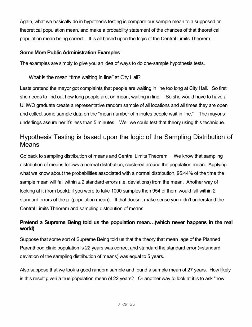
Again, what we basically do in hypothesis testing is compare our sample mean to a supposed or

theoretical population mean, and make a probability statement of the chances of that theoretical

population mean being correct. It is all based upon the logic of the Central Limits Theorem.

Some More Public Administration Examples

The examples are simply to give you an idea of ways to do one-sample hypothesis tests.

What is the mean “time waiting in line” at City Hall?

Lests pretend the mayor got complaints that people are waiting in line too long at City Hall. So first

she needs to find out how long people are, on mean, waiting in line. So she would have to have a

UHWO graduate create a representative random sample of all locations and all times they are open

and collect some sample data on the “mean number of minutes people wait in line.” The mayor’s

underlings assure her it’s less than 5 minutes. Well we could test that theory using this technique.

Hypothesis Testing is based upon the logic of the Sampling Distribution of Means

Go back to sampling distribution of means and Central Limits Theorem. We know that sampling

distribution of means follows a normal distribution, clustered around the population mean. Applying

what we know about the probabilities associated with a normal distribution, 95.44% of the time the

sample mean will fall within ± 2 standard errors (i.e. deviations) from the mean. Another way of

looking at it (from book): if you were to take 1000 samples then 954 of them would fall within 2

standard errors of the µ (population mean). If that doesn’t make sense you didn’t understand the

Central Limits Theorem and sampling distribution of means.

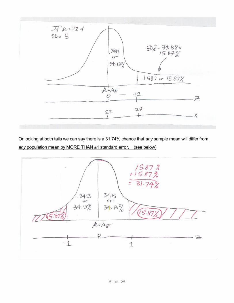
Pretend a Supreme Being told us the population mean…(which never happens in the real world)

Suppose that some sort of Supreme Being told us that the theory that mean age of the Planned

Parenthood clinic population is 22 years was correct and standard the standard error (=standard

deviation of the sampling distribution of means) was equal to 5 years.

Also suppose that we took a good random sample and found a sample mean of 27 years. How likely

is this result given a true population mean of 22 years? Or another way to look at it is to ask "how

4 OF 25

likely was it for us to get such a difference (of 5 years) between our hypothesized population mean

and our sample mean?

To answer this question we must convert the difference between our sample mean and hypothesized

population mean into "standardized" standard deviations -- similar to z or t scores! We use this

formula:

TR = x

Hoxσµ−

Now, look at the z formula: z= σµ−x

Don't these two formulas look "hauntingly" similar? They both do the same thing -- create

"standardized" scores for standard deviation units.

Applying probabilities Associated with the Sampling Dist. of Means

Well in this case we can plug the information into the formula and or look at it with common sense and

we find out that 27 years represents one standard deviation, unit, or error from the hypothesized

sample mean of 22 years.

“z”=

€

27 − 225

=55

=1 The area for (z=1)=.34.13%.

Using the properties of the normal curve we can see there is a 15.87% chance that sample mean will

be greater than the population mean by 1 or more standard errors. (see below)

5 OF 25

Or looking at both tails we can say there is a 31.74% chance that any sample mean will differ from

any population mean by MORE THAN ±1 standard error. (see below)

6 OF 25

If our sample mean was 32 years (still with a population mean of 22 years and a SD = 5 years ) what

are the chances of that occurring?

“z”=

€

32 − 225

=105

= 2 Well, z(2)=47.72% (95.44% in middle and 2.28% in each tail). Well, there is

a 4.56% chance of getting this sample mean when the true population mean is 22 years. (see below)

If we didn’t know the true population mean we could say that there is a 95.44% chance of the original

estimate of being wrong. If we got a sample mean of 32 years and concluded that theory that the true

population mean age is equal to 33 was incorrect, we would actually be wrong! But that is not really

the point! There was a pretty small chance of us being wrong.

7 OF 25

Think about the logic of the sampling distribution of means You do not know which sample mean you

will get, but there is only a 4.56% chance that you would get a sample mean that was plus or minus 2

SD’s away from the grand mean! There is less than a 5 % chance that this would happen. So you

could say that there is a 95.44% chance that the hypothetical mean of 22 years is incorrect and that

our sample mean comes from a WHOLE DIFFERENT sampling distribution of means WITH A

DIFFERENT GRAND MEAN. In our case, we could make this statement with 95.44% confidence of

being right. That means there would be a 4.56% chance of being wrong.

Supreme Beings don’t tell us the population mean in the real world

In the real world Supreme Beings do not tell us what the real population mean is. We just pretended

we knew that the real population mean was = 22 years in the example above. In the real world we

have no idea what the real population mean is. We have to estimate the population mean based

upon a sample mean! If you can make an estimate of the real population mean and be at least 95%

confident of being right, then we do so in statistics. In fact, the “standard of the industry” in statistics is

to have at least a 95% chance of being right.

Statisticians usually accept a 5% or 1% of being wrong in social sciences. Or conversely there is a

95% or 99% confidence of being right.

Another way to look at it is the logic of the Central Limits Theorem. Statistical theory says that if the

sample mean falls greater than ± 1.96 standard errors away from the hypothesized population mean

(this comes from sampling distribution of means) then there is only a 5% chance that our sample

mean belongs to such a population. Thus our sample must not belong to that population at all – it

must belong to a whole “other” population with a whole different sampling distribution of means [and

that sampling distribution of means has a different grand mean than our theory]! We can be 95%

confident of this statement.

A note about 95% (α=.05) and 99% (α=.01)

These are totally arbitrary! They are just accepted as the “standard of the industry.” It is an arbitrary

cut off point that signifies “statistical significance.” All “scientific proof” is based upon statistical

significance! Think about that for a moment!

So from a philosophical standpoint, science is just a “new” belief system based upon chance! In the

past we may have climbed the snowcapped mountain to ask the religious shaman, “What are the

8 OF 25

great truths of the world?” Now, I would like to suggest, we have entered a “rational” phase where we

go to the scientist for the great truths of the world.

Even if the data is collected in the finest possible way, the best any scientific study can say that they

are 95% or 99% confident something is true, but there is always a probability of error. Now, a 5 or 1%

chance of error aint bad, and in fact that’s pretty good! Don’t fall into the armchair cynics’ trap and

throw out the “baby with the bath water.” For example, for certain types of research questions, the

social scientific method provides information that is oodles and oodles better than mere

philosophizing under the oak tree or from the Lazy-boy recliner in front of the TV. For questions like

“Is that drug safe to take?” and “How long will the ‘Jesus nut’ on the helicopter rotor last?”, I

personally feel far more comfortable with a rational approach based upon probability.

Social research does not produce perfect knowledge, but it probably does produce better knowledge

than mere philosophy. It is certainly more objective and very rational. However, scientific proof based

upon sampling utilizes the belief system of chance or probability. Whether or not that leads to “truth”

is something everyone must decide for himself or herself.

Type I error

So in terms of hypothesis testing, when we choose a 95% confidence interval or an “alpha” of .05, we

are accepting a 5% chance of being wrong. Or to put it more precisely, when we choose an alpha of

5%, we are accepting a 5% chance of saying the educated guess is wrong when, in reality it is right. So type 1 error is saying a hypothesis is wrong when “in reality” it is correct. Or it is the probability of incorrectly rejecting a correct null hypothesis.

REALITY

Statisticians Guess

hypoth right hypoth wrong

hypoth right correct guess! error! hypoth wrong error! Correct guess! Or, to put it into “statistician speak”:

REALITY Statisticians Guess

hypoth right hypoth wrong

hypoth right correct guess! type II error

9 OF 25

hypoth wrong type I error Correct guess! Thus, when we chose an α =.05 (or want 95% confidence), we are accepting a 5% chance of type I

error.

Setting up Null and Alternative Hypothesis

Setting up the null and alternative (or research) hypothesis is sort of “bassackwards.” What you want

to “prove” you put in the alternative (or research) hypothesis and you “prove” it by rejecting its exact

opposite. It’s as if you say, “Well, if I can disprove the exact opposite of what I want to prove then I

can conclude that my theory is right.” Remember how science works: one of the ways a person

makes a name for herself is by proving other people’s theories wrong. “So and so said this should be

the population mean, but I have shown that cannot be the case and therefore we must amend so and

so’s theory.” Kind of weird, but the best way to get over it is to practice doing a whole bunch of them.

For example say I want to prove that the population mean is different than 22 (note I don’t care which

way it’s different) then here is how I set up the null and alternative hypothesis:

Ho: This is the symbolism for the NULL hypothesis

H1: This is the symbolism for the ALTERNATIVE (or research) hypothesis

So below is the null and alternative (or research) hypothesis to prove that the population mean is

different than 22:

Ho: µ = 22 H1: µ ≠ 22

Let’s do another example. Pretend I want to prove that the population mean is different than 30 (note

I don’t care which way it’s different) then here is how I set up the null and alternative hypothesis:

Ho: µ = 30 H1: µ ≠ 30

Or I want to prove that the mean age of UH Manoa students is below 25. Or the mean age of NBA

players is less than 30.

Ho: µ ≥ 25 H1: µ < 25

Ho: µ ≥ 30 H1: µ < 30

10 OF 25

The 7 Steps to Classical Hypothesis Testing

Note: in all of the examples in this lecture we end up rejecting the null hypothesis. For an example of when you fail to reject the null hypothesis [FTR] please see the very first practice problem in lecture 17b: practice problems (17b_practice.pdf).

n>30 and σ is unknown

All students who want to go to Law School have to take a test called the LSAT – it’s like the SAT but

for wanna-be lawyers. There are private programs that will allow you to pay a fee and take prep class

– claiming that their prep class will help you improve your LSAT score. You are working for a public

university that wants to start its own LSAT prep program and prove that the private programs are not

as good as they claim. [That means that people would want to come to your public university for the

same service!]

“Blu Get Clues” is a LSAT prep school. Blu’s school states that mean LSAT score of their graduates

is1200. You do a study for your public university and take a random sample of 100 students and

come up with the following information: n=100, s=100, x =1180

Test the theory that the mean LSAT test score is equal to 1200 or conversely, to try to prove their

mean LSAT not equal to 1200. (see step 1 below)

Step 1: State the null and alternative (or research) hypothesis (H0 and H1).

Basic one sample two tailed test:

H0: µ = theoretical population mean

H1: µ ≠ theoretical population mean

So for our problem:

H0: µ = 1200

H1: µ ≠ 1200

Step 2: State level of significance or α “alpha.”

For this example we’ll use alpha =.05

11 OF 25

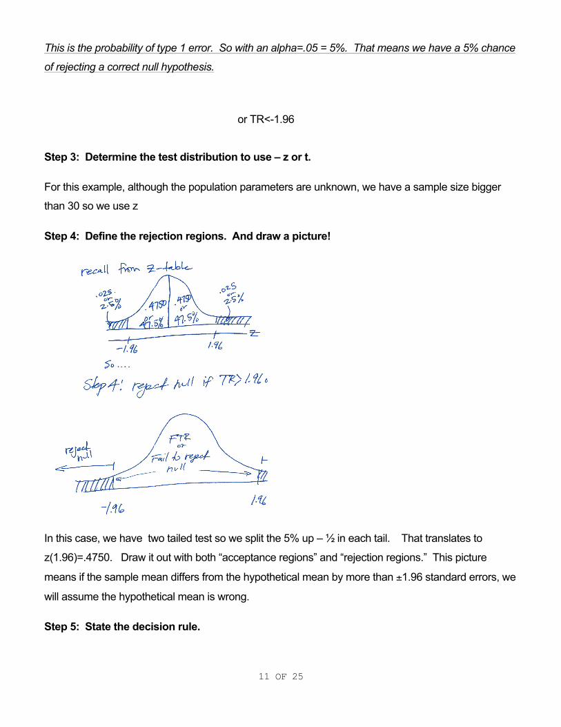
This is the probability of type 1 error. So with an alpha=.05 = 5%. That means we have a 5% chance

of rejecting a correct null hypothesis.

Step 3: Determine the test distribution to use – z or t.

For this example, although the population parameters are unknown, we have a sample size bigger

than 30 so we use z

Step 4: Define the rejection regions. And draw a picture!

In this case, we have two tailed test so we split the 5% up – ½ in each tail. That translates to

z(1.96)=.4750. Draw it out with both “acceptance regions” and “rejection regions.” This picture

means if the sample mean differs from the hypothetical mean by more than ±1.96 standard errors, we

will assume the hypothetical mean is wrong.

Step 5: State the decision rule.

or TR<-1.96

12 OF 25

Reject the null if the TR >1.96 or TR<-1.96, otherwise FTR.

Step 6: Perform necessary calculations on data and compute TR value.

In this case TR = x

Hoxσµ−

where xσ =ns

(Note I used infinite formula for simplicity. But this population is probably not infinite.)

xσ =ns =

€

100100

=10010

=10

TR = = =

€

−2010

= −2

SIDE NOTE about “TR” in these lecture notes: I use TR to refer to the “test ratio” or formula that is used in all

hypothesis tests of means:

x

Hoxσµ−

Some books put a z in front of the formula when n>30 and you use the z table: z = x

Hoxσµ−

and put a t in front of the

formula when n<30 you use the t-table: t=x

Hoxσµ−

Remember the formula is exactly the same regardless of whether you call it TR, z or t!!!

x

Hoxσµ−

€

1180 −1200

10

13 OF 25

Step 7: Compare TR value with the decision rule and make a statistical decision. (Write out decision in English! -- my addition)

-2 falls in rejection region. Therefore we reject null and conclude that the company’s statement is

incorrect. Their mean LSAT score of prep course graduates is not 1200. Notice: we don’t say

which way they are wrong, we just know that the hypothesized population mean of 1200 is probably

wrong. (We are at least 95% confident of this statement.)

So there is less than a 5% chance that a sample mean of 1180 could come from a sampling

distribution of means where the population mean or grand mean =1200.

p-value in plain English

We learn to calculate the p-value (by hand) in the lecture 17a: computing p-values (17a_p-value.pdf)

and from SPSS in lecture 17c: SPSS output (17c_SPSS.pdf), but I want you to get comfortable

knowing that the p-value comes from the TR in step six and it gives us the “probability of incorrectly

rejecting the null.”

The SPSS p value for this TR value would be p=.0456 or 4.56%. In plain English this means you can

reject the null can conclude that mean LSAT score of prep course graduates is not equal to1200 with

a 4.56%. chance of being wrong.

What is the wording when we fail to reject the null hypothesis?


But as a primer, when we fail to reject the null hypothesis we say “Insufficient evidence to reject theory that __________ “ [insert Ho in plain English.] You do not “conclude” null, so much as you can only say “insufficient evidence to reject theory in null” which relates to the way science progresses. Until there is evidence to reject the theory the theory stands. We are not 95% confident or anything like that. So in the problem immediately above pretend we failed to reject the null hypothesis. What would the

language be?

14 OF 25

H0: µ = 1200 H1: µ not = 1200 Pretending we failed to reject null we would say, “Insufficient evidence to reject theory that the population mean LSAT score of prep course graduates is equal to1200.” So on the take home exams if you fail to reject the null hypothesis [this will happen a lot in test 3 and test 4] use this language template if you will, “Insufficient evidence to reject theory that __________ “ [insert Ho in plain English.]

15 OF 25

One- Tailed Hypothesis Test of Means: Could “Blu Get Clues” be engaged in “false advertising?”

Pretend you graduated from UHWO and now have a job at the Federal Trade Commission – the

Federal Agency that investigates claims of false advertising. You tell your boss about “Blu Get Clues”

and the study you did for your senior project.

What if we wanted to see ”Blu Get Clues” was overstating their claim and is guilty of false advertising?

What if their “true population mean score” is really less than 1200? You are able use the same

information as above: n=100, s=100, x =1180

So we test the theory that the mean LSAT test score is greater than or equal to 1200 or conversely, to

try to prove their mean LSAT less than 1200. (see step 1 below)

One Sample one-tailed tests

For this question we do a “one sample left tailed one-tailed test.”

H0: µ ≥ ?

H1: µ < ? left tailed test! Alternative points to rejection region

(There is also a “one sample right-tailed one-tailed test.”)

H0: µ ≤ ?

H1: µ > ? right tailed test! Alternative points to rejection region


H0: µ ≥ 1200 H1: µ < 1200 Step 2: State level of significance or α “alpha.”


16 OF 25


For this example, although the population parameters are unknown, we have a sample size bigger

than 30 so we use z


In this case, we have a one tailed test so we put all 5% into the “left tail.” Z(-1.645) Draw it out with

both “acceptance regions” and “rejection regions.” This picture means if the sample mean differs from

the hypothetical mean by less than -1.645 standard errors, we will assume the hypothetical mean is

wrong.

17 OF 25

Note about rejection regions for one tailed tests:

Here you need to pay attention to whether or not your TR falls in the tail that has the rejection region. Recall that

in a one-tailed test the “arrow” in the bottom or alternative (or research) hypothesis “points” to the rejection

region.

Negative tail rejection regions

H0: µ ≥ 1200 H1: µ < 1200

Here H1: µ < 1200, so the “arrow” in the bottom or alternative (or research) hypothesis (H1) points to the left. The rejection region is in the left or negative part of the curve.

Positive tail rejection regions

H0: µ ≤ 1200 H1: µ > 1200

Here H1: µ > 1200, so the “arrow” in the bottom or alternative (or research) hypothesis (H1) points to the right. The rejection region is in the right or positive part of the curve.


18 OF 25

Reject the null if the TR<-1.645, otherwise FTR.


In this case TR = x

Hoxσµ−

where xσ =ns

(Note I used infinite formula for simplicity. But this population is probably not infinite.)

xσ =ns =

€

100100

TR = x

Hoxσµ−

=

€

1180 −120010

=

€

−2010

= −2


TR falls in rejection region: reject null and conclude alternative. Conclude the mean LSAT score of

“Blu Get Clues” graduates is less than 1200. We are at least 95% confident of this statement.

So there is less than a 5% chance that a sample mean of 1180 could come from a sampling

distribution of means where the population mean or grand mean = 1200.

p-value

We learn to calculate the p-value (by hand) in the lecture 17a: computing p-values (17a_p-value.pdf)

and from SPSS in lecture 17c: SPSS output (17c_SPSS.pdf), but I want you to get comfortable

knowing that the p-value comes from the TR in step six and it gives us the “probability of incorrectly

rejecting the null.”

The SPSS p value for this TR value would be p=.0228 or 2.28%. In plain English this means you can

reject the null can conclude that mean LSAT score of prep course graduates is not equal to1200 with

a 2.28%. chance of being wrong.

19 OF 25

When n<30 use t table! In this section we will do a one and two tailed tests when n<30 and we have to use the t table. Most

of you will have to do this sort of problem on your take home test as your n or sample size is less than

30!

Two tailed test

Hopefully you learned above that two tailed tests are not as useful as one tailed tests. However two

tailed tests are generally the way to introduce the concept.

A Big Boss in the City and County agency has heard that one of his departments is receiving, on

mean 16 complaints a month. The Big Boss is going to collect some data to see if he needs to

replace the manager of the department. If the complaints are too high he will fire the manager.

Thus the Big Boss will test the theory that the mean number of complaints per month is equal to 16.

Conversely he will try to prove that the mean number of complaints per month is not equal to 16.

(Again a two tailed test is sort of useless to the Big Boss. The Big Boss would like to prove that the

mean number of complaints is more than 16, because if it is less than 16, he should not fire the

manager. Please bear with me Below this example I do a one tailed test that “makes sense.”)

Here are the data

Random sample of n=10 months, s= 2.05 complaints, =18 complaints


H0: µ = 16 complaints per month H1: H1: µ ≠ 16 complaints per month Step 2: State level of significance or α “alpha.”



x

20 OF 25

n<30 use t and assume that the mean number of complaints in the population was normally

distributed. In this case, we have a two tailed test so we put all half of the error (or alpha) in step 2

into each tail.

df =n-1 10-1=9 with df=9 and α=.025 from t table rejection area = 2.262

Step 4: Define the rejection regions. (sorry no picture)

In this case, we have a two tailed test so we put all half of the error (or alpha) in step 2 into each tail.

This means if the sample mean differs from the hypothetical mean by greater than 2.262 or less than

-2.262 standard errors, we will assume the hypothetical mean is wrong.


Reject the null if the TR>2.262 or if TR< -2.262 otherwise FTR.


In this case t = =

€

18 −162.05 / 10

=

€

2.64979

= 3.078

=

x

Hoxσµ−

xσ ns

21 OF 25

SPSS output and p value below


Reject null. There is sufficient evidence at the .05 level of significance to reject the hypothesis that the

mean number of complaints is not equal to 16 per month. Or he can conclude that the mean number

of complaints per month is not equal to 16 per month with less than a 5% chance of error. (The 5%

chance of error is the alpha in step 2.) The big boss has “statistically significant” evidence that will

allow him to fire the manager (and there is less than a 5% chance of the firing being unjustified.)

p-value

NOTE! We will not compute p value by hand when n<30 (and we use t table) in this class. This is because of the way the t-table in the book is structured. A better t table would allow for hand computations. But in this class, when we use the t table we will rely on SPSS to compute the p-value. I show how to compute p value in lecture 17c: SPSS output (17c_SPSS.pdf), but according to spss p= .013 or 1.3%. In plain English, the Big Boss can conclude that the mean number of complaints per month is not equal to 16, but there is a 1.3 % chance that his conclusion is wrong or in error. Note that in a two tailed test the Big Boss can only prove that mean number of complaints is not equal to 16. He cannot say whether or not the mean number of complaints is more than or less than 16 – kind of useless yeah?

22 OF 25

One tailed test

A Big Boss in the City and County agency has heard that one of his departments is receiving, on

mean 16 complaints a month. The Big Boss is going to collect some data to see if he needs to

replace the manager of the department. If the complaints are too high he will fire the manager.

The manager’s contract states that if the mean number of complaints are greater than 16 per month,

then job performance is unsatisfactory and grounds for dismissal. If the Big Boss can prove that

µ>16 per month, he can fire the manager. (Hopefully now you see why a one tailed test is more

useful given this example!)

Thus test the theory that the mean number of complaints per month is less than or equal to 16.

Conversely try to prove that the mean number of complaints per month is greater than 16.

Here are the data

Random sample of n=10 months, s= 2.05 complaints, x =18 complaints


H0: µ ≤ 16 complaints per month H1: µ > 16 complaints per month Step 2: State level of significance or α “alpha.”

For this example we’ll use alpha =.01. Note that we have been using alpha =.05 or 5%. Here I

change it to .01 or 1%!


n<30 use t and assume that he population from which we sampled was normally distributed.

df =n-1 10-1=9 with df=9 and α=.01 from t table rejection area = 2.821

23 OF 25


In this case, we have a one tailed test so we put all 1% into the “right tail.” ( t>2.821) This picture

means if the sample mean differs from the hypothetical mean by more than 2.821 standard errors, we

will assume the hypothetical mean is wrong.


Reject the null if the t>2.821 otherwise FTR.


In this case t =x

Hoxσµ−

=

€

18 −162.05 / 10

=

€

2.64979

= 3.078

xσ =ns

SPSS output and p value below

24 OF 25


Reject null. There is sufficient evidence at the .01 level of significance to reject the hypothesis that the

mean number of complaints is greater than 16 per month. Or he can conclude that the mean

number of complaints per month is greater than 16 with less than a 1% chance of error. (The 1%

chance of error is the alpha in step 2.) The big boss has “statistically significant” evidence that will

allow him to fire the manager (and there is less than a 1% chance of the firing being unjustified.)

p-value

NOTE! We will not compute p value by hand when n<30 (and we use t table) in this class. This is because of the way the t-table in the book is structured. A better t table would allow for hand computations. But in this class, when we use the t table we will rely on SPSS to compute the p-value. I show how to compute p value in lecture 17c: SPSS output (17c_SPSS.pdf), but according to spss p= .013/2 or p=0.0065, or 0.65%. In plain English, the Big Boss can conclude that the mean number of complaints per month is greater than 16, but there is a 0.65% chance that his conclusion is wrong or in error.

What is the wording when we fail to reject the null hypothesis?


25 OF 25

But as a primer, when we fail to reject the null hypothesis we say “Insufficient evidence to reject theory that __________ “ [insert Ho in plain English.] You do not “conclude” null, so much as you can only say “insufficient evidence to reject theory in null” which relates to the way science progresses. Until there is evidence to reject the theory the theory stands. We are not 95% confident or anything like that. So in the problem immediately above pretend we failed to reject the null hypothesis. What would the

language be?

H0: µ 16 complaints per month H1: µ > 16 complaints per month “Insufficient evidence to reject theory that the population mean number or monthly complaints is less than or equal to 16.”

Practice

Practice problems can be found in lecture 17b “practice problems for lecture 17” (17b_practice.pdf)

≤

lecture 17 one sample hypothesis testing - laulima ... 17: one sample hypothesis test of means (or t...

Documents