Hypothesis Testing with the Bootstrap

Noa Haas Statistics M.Sc. Seminar, Spring 2017 Bootstrap and Resampling Methods

Bootstrap Hypothesis Testing

A bootstrap hypothesis test starts with a test statistic - 𝑡(𝒙) (not necessary an estimate of a parameter).

We seek an achieved significance level 𝐴𝑆𝐿 = 𝑃𝑟𝑜𝑏𝐻0

𝑡 𝒙∗ ≥ 𝑡(𝒙)

Where the random variable 𝒙∗ has a distribution specified by the null hypothesis 𝐻0 - denote as 𝐹0.

Bootstrap hypothesis testing uses a “plug-in” style to estimate 𝐹0.

The Two-Sample Problem

We observe two independent random samples:

And we wish to test the null hypothesis of no difference between F and G,

𝐹 → 𝒛 = 𝑧1, 𝑧2, … , 𝑧𝑛 𝑖𝑛𝑑𝑒𝑝𝑒𝑛𝑑𝑒𝑛𝑡𝑙𝑦 𝑜𝑓 𝐺 → 𝒚 = 𝑦1, 𝑦2, … , 𝑦𝑚

𝐻0: 𝐹 = 𝐺

Bootstrap Hypothesis Testing 𝐹 = 𝐺

• Denote the combined sample by 𝒙, and its empirical distribution by 𝐹 0.

• Under 𝐻0, 𝐹 0 provides a non parametric estimate for the common population that gave rise to both 𝒛 and 𝒚.

1. Draw 𝑩 samples of size 𝑛 + 𝑚 with replacement from 𝒙. Call the first n observations 𝒛∗ and the remaining 𝑚 – 𝒚∗

2. Evaluate 𝑡(∙) on each sample - 𝑡(𝒙∗𝒃)

3. Approximate 𝐴𝑆𝐿𝑏𝑜𝑜𝑡 by

𝐴𝑆𝐿 𝑏𝑜𝑜𝑡 = # 𝑡 𝒙∗𝒃 ≥ 𝑡 𝒙 /𝐵

* In the case that large values of 𝑡(𝒙∗𝒃) are evidence against 𝐻0

Bootstrap Hypothesis Testing 𝐹 = 𝐺 on the Mouse Data A histogram of bootstrap replications of

𝑡 𝒙 = 𝑧 − 𝑦 for testing 𝐻0: 𝐹 = 𝐺 on the mouse data. The proportion of values greater than 30.63 is .121. Calculating

𝑡 𝒙 =𝑧 − 𝑦

𝜎 1 𝑛 + 1 𝑚

(approximate pivotal) for the same replications produced

𝐴𝑆𝐿 𝑏𝑜𝑜𝑡 = .128

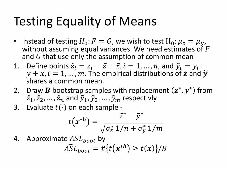
Testing Equality of Means

• Instead of testing 𝐻0: 𝐹 = 𝐺, we wish to test H0: 𝜇𝑧 = 𝜇𝑦, without assuming equal variances. We need estimates of 𝐹 and 𝐺 that use only the assumption of common mean

1. Define points 𝑧 𝑖 = 𝑧𝑖 − 𝑧 + 𝑥 , 𝑖 = 1, … , 𝑛, and 𝑦 𝑖 = 𝑦𝑖 −𝑦 + 𝑥 , 𝑖 = 1, … , 𝑚. The empirical distributions of 𝒛 and 𝒚 shares a common mean.

2. Draw 𝑩 bootstrap samples with replacement 𝒛∗, 𝒚∗ from 𝑧 1, 𝑧 2, … , 𝑧 𝑛 and 𝑦 1, 𝑦 2, … , 𝑦 𝑚 respectivly

3. Evaluate 𝑡(∙) on each sample -

𝑡 𝒙∗𝒃 =𝑧 ∗ − 𝑦 ∗

𝜎 𝑧∗ 1 𝑛 + 𝜎 𝑦

∗ 1 𝑚

4. Approximate 𝐴𝑆𝐿𝑏𝑜𝑜𝑡 by

𝐴𝑆𝐿 𝑏𝑜𝑜𝑡 = # 𝑡 𝒙∗𝒃 ≥ 𝑡 𝒙 /𝐵

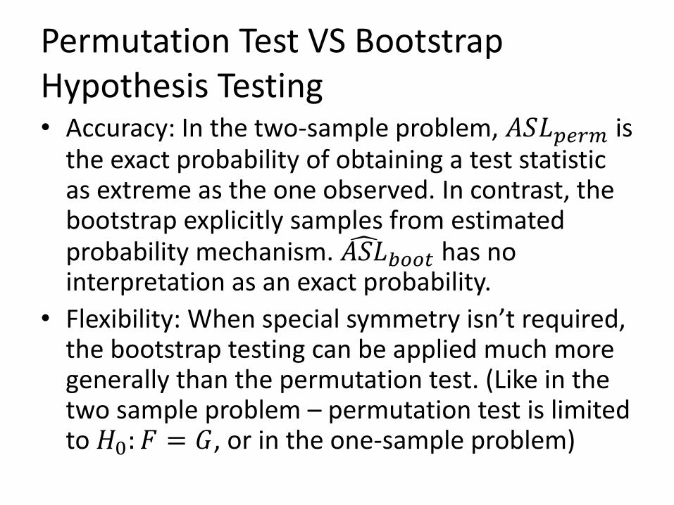
Permutation Test VS Bootstrap Hypothesis Testing • Accuracy: In the two-sample problem, 𝐴𝑆𝐿𝑝𝑒𝑟𝑚 is

the exact probability of obtaining a test statistic as extreme as the one observed. In contrast, the bootstrap explicitly samples from estimated probability mechanism. 𝐴𝑆𝐿

𝑏𝑜𝑜𝑡 has no interpretation as an exact probability.

• Flexibility: When special symmetry isn’t required, the bootstrap testing can be applied much more generally than the permutation test. (Like in the two sample problem – permutation test is limited to 𝐻0: 𝐹 = 𝐺, or in the one-sample problem)

The One-Sample Problem

We observe a random sample:

And we wish to test whether the mean of the population equals to some predetermine value 𝜇0 −

𝐹 → 𝒛 = 𝑧1, 𝑧2, … , 𝑧𝑛

𝐻0: 𝜇𝑧 = 𝜇0

Bootstrap Hypothesis Testing 𝜇𝑧 = 𝜇0

What is the appropriate way to estimate the null distribution?

The empirical distribution 𝐹 is not an appropriate estimation, because it does not obey 𝐻0.

As before, we can use the empirical distribution of the points:

𝑧 𝑖 = 𝑧𝑖 − 𝑧 + 𝜇0, 𝑖 = 1, … , 𝑛

Which has a mean of 𝜇0.

Bootstrap Hypothesis Testing 𝜇𝑧 = 𝜇0

The test will be based on the approximate

distribution of the test statistic 𝑡 𝒛 =𝑧 −𝜇0

𝜎 / 𝑛

We sample 𝑩 times 𝑧 1∗, … , 𝑧 𝑛

∗ with replacement from 𝑧 1, … , 𝑧 𝑛, and for each sample compute

𝑡 𝒛 ∗ =𝑧 − 𝜇0

𝜎 / 𝑛

And the estimated ASL is given by

𝐴𝑆𝐿 𝑏𝑜𝑜𝑡 = # 𝑡 𝒛 ∗𝒃 ≥ 𝑡 𝒛 /𝐵

* In the case that large values of 𝑡 𝒛 ∗𝒃 are evidence against 𝐻0

Testing 𝜇𝑧 = 𝜇0 on the Mouse Data

Taking 𝜇0 = 129, the observed value of the test statistic is

𝑡 𝒛 =86.9 − 129

66.8/ 7= −1.67

(When estimating 𝜎 with the unbiased estimator for standard deviation). For 94 of 1000 bootstrap samples, 𝑡 𝒛 ∗ was smaller than -1.67, and therefor

𝐴𝑆𝐿 𝑏𝑜𝑜𝑡 = .094

For reference, the student’s t-test result for the same null hypothesis on that data gives us

𝐴𝑆𝐿 = 𝑃𝑟𝑜𝑏 𝑡6 < −42.1

66.8/ 7= 0.07

Testing Multimodality of a Population

A mode is defined to be a local maximum or “bump” of the population density

The data: 𝑥1, … , 𝑥485 Mexican stamps’ thickness from 1872.

The number of modes is suggestive of the number of distinct type of paper used in the printing.

Testing Multimodality of a Population

Since the histogram is not smooth, it is difficult to tell from it whether there are more than one mode.

A Gaussian kernel density with window size ℎ estimate can be used in order to obtain a smoother estimate:

𝑓 𝑡; ℎ =1

𝑛ℎ 𝜙

𝑡 − 𝑥𝑖

ℎ

𝑛

𝑖=1

As 𝒉 increases, the number of modes in the density estimate is non-increasing

Testing Multimodality of a Population

The null hypothesis: 𝐻0: 𝑛𝑢𝑚𝑏𝑒𝑟 𝑜𝑓 𝑚𝑜𝑑𝑒𝑠 = 1

Versus 𝑛𝑢𝑚𝑏𝑒𝑟 𝑜𝑓 𝑚𝑜𝑑𝑒𝑠 > 1. Since the number of modes decreases as

ℎ increases, there is a smallest value of ℎ such that 𝑓 𝑡; ℎ has one mode.

Call it ℎ 1. In our case, ℎ 1 ≈ .0068.

Testing Multimodality of a Population

It seems reasonable to use 𝑓 (𝑡; ℎ 1) as the estimated null distribution for our test of 𝐻0. It is the density estimate that uses least amount of smoothing among all estimated with one mode (conservative).

A small adjustment to 𝑓 is needed because the formula artificially

increases the variance of the estimate with ℎ 12. Let 𝑔 ∙; ℎ 1 be the rescale

estimate, that imposes variance equal to the sample variance.

A natural choice for a test statistic is ℎ 1 - a large value of ℎ 1 is evidence against 𝐻0.

Putting all of this together, the achieved significance level is

𝐴𝑆𝐿𝑏𝑜𝑜𝑡 = 𝑃𝑟𝑜𝑏𝑔 ∙;ℎ 1ℎ 1

∗ > ℎ 1

Where each bootstrap sample 𝒙∗ is drawn from 𝑔 ∙; ℎ 1

Testing Multimodality of a Population

The sampling from 𝑔 ∙; ℎ 1 is given by:

𝑥𝑖∗ = 𝑥 + 1 + ℎ 1

2 𝜎 2 −

12 𝑦𝑖

∗ − 𝑥 + ℎ 1𝜖𝑖 ; 𝑖 = 1, … , 𝑛

Where 𝑦1∗, … , 𝑦𝑛

∗ are sampled with replacement from 𝑥1, … , 𝑥𝑛, and 𝜖𝑖 are standard normal random variables. (called smoothed bootstrap)

In the stamps data, out of 500 bootstrap samples, none had

ℎ 1∗ > .0068, so 𝐴𝑆𝐿

𝑏𝑜𝑜𝑡 = 0.

The results can be interpreted in sequential manner, moving on to higher values of the least amount of modes. (Silverman 1981)

When testing the same for 𝐻0: 𝑛𝑢𝑚𝑏𝑒𝑟 𝑜𝑓 𝑚𝑜𝑑𝑒𝑠 = 2, 146

samples out of 500 had ℎ 2∗ > .0033, which translates to 𝐴𝑆𝐿

𝑏𝑜𝑜𝑡

= 0.292.

In our case, the inference process will end here.

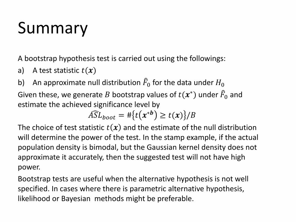
Summary

A bootstrap hypothesis test is carried out using the followings:

a) A test statistic 𝑡(𝒙)

b) An approximate null distribution 𝐹 0 for the data under 𝐻0

Given these, we generate 𝐵 bootstrap values of 𝑡(𝒙∗) under 𝐹 0 and estimate the achieved significance level by

𝐴𝑆𝐿 𝑏𝑜𝑜𝑡 = # 𝑡 𝒙∗𝒃 ≥ 𝑡(𝒙) /𝐵

The choice of test statistic 𝑡 𝒙 and the estimate of the null distribution will determine the power of the test. In the stamp example, if the actual population density is bimodal, but the Gaussian kernel density does not approximate it accurately, then the suggested test will not have high power.

Bootstrap tests are useful when the alternative hypothesis is not well specified. In cases where there is parametric alternative hypothesis, likelihood or Bayesian methods might be preferable.