daniel lawson october 2014 testing’ slidesmadjl/hypothesistesting.pdf · the simple z test the z...
TRANSCRIPT
Hypothesis Testing
Daniel Lawson
Wellcome Trust Sir Henry Dale Research FellowIEU, University of Bristol
Visiting researcher at the University of Oxford
October 2014Gently adapted from David Steinsaltz’s 2013 ‘hypothesis
testing’ slides
1 / 126
Table of ContentsBackground
The Z testThe simple Z testThe Z test for proportionsThe Z test for the difference between meansZ test for the difference between proportions
The t testThe simple t testThe Matched sample t testMatched sample t test
The χ2 testThe χ2 test
Non-parametric testsWhy we need non-parametric testsMann-Whitney U testPaired value tests
The menagerie of tests2 / 126

Section 1
Background
3 / 126
The testing paradigm
Significance testing is about rejecting a null model.
I We have a research hypothesis, which helps define thealternative hypothesis
I The null model is our best explanation of the data withoutthat hypothesis
I We see if the null model ‘fits’ the data with a test
I We will ‘test’ all of the assumptions of the null together!
I i.e. we won’t know which assumption failed
I If we reject the null, we hope our alternative hypothesis is theexplanation!
I Confounding by some unaccounted process is the mostcommon reason for incorrectly accepted alternatives.
I If you can’t account for all reasonable confounders, there is nopoint doing the test!
4 / 126
Decisions and hypothesis testing
One reason for HT is to make decisions. It is biased against thealternative, so that if the null is rejected we are fairly certain thatis not a mistake.
I Example: A new vaccine.
I Null hypothesis: it doesn’t work.
I Alternative: it does. So use it!
It is important to control the probability that we decide it works!(But we aren’t taking into account the cost of getting it wrong.)
5 / 126

Types of error
I Type I: We reject the null hypothesis, but its really true
I Type II: We retain the null, but it isn’t true
These are very different!In many fields, no null hypothesis can be true.This leads to the question: do we have power to reject the null?In this case, standard hypothesis testing can be useless fordemonstrating a specific alternative.
6 / 126

The Confusion Matrix
What is true?
What we do?Reject Null Retain null
null False positive True negativeType I error
alternative True positive False negativeType II error
Power = true positive ratefalse negative rate for a given false positive rate α.
7 / 126
Example: Spam Filter
Spam filters look at incoming email, and use statistical models tocompute the probability that a real message would have certainfeatures. If the probability is too low, it goes directly in the bin.
Null hypothesis: Real message.Alternative: Spam.
Then a Type I error is
1. A spam message that gets through the filter;
2. An email from your friend that gets junked?
Type I = falsely rejecting the nullAnswer: 2
8 / 126

Example: Spam Filter
Spam filters look at incoming email, and use statistical models tocompute the probability that a real message would have certainfeatures. If the probability is too low, it goes directly in the bin.
Null hypothesis: Real message.Alternative: Spam.
Then a Type I error is
1. A spam message that gets through the filter;
2. An email from your friend that gets junked?
Type I = falsely rejecting the null
Answer: 2
8 / 126

Example: Spam Filter
Spam filters look at incoming email, and use statistical models tocompute the probability that a real message would have certainfeatures. If the probability is too low, it goes directly in the bin.
Null hypothesis: Real message.Alternative: Spam.
Then a Type I error is
1. A spam message that gets through the filter;
2. An email from your friend that gets junked?
Type I = falsely rejecting the nullAnswer: 2
8 / 126
Example: Criminal Trial
Juries weigh the evidence, and decide how likely the evidencewould be if the defendant were innocent.Null hypothesis: Defendant is innocent.Alternative: Defendant is guilty.
Then a Type II error is
1. A guilty defendant set free;
2. An innocent defendant convicted.
Type II = falsely rejecting the alternativeAnswer: 1
9 / 126
Example: Criminal Trial
Juries weigh the evidence, and decide how likely the evidencewould be if the defendant were innocent.Null hypothesis: Defendant is innocent.Alternative: Defendant is guilty.
Then a Type II error is
1. A guilty defendant set free;
2. An innocent defendant convicted.
Type II = falsely rejecting the alternative
Answer: 1
9 / 126
Example: Criminal Trial
Juries weigh the evidence, and decide how likely the evidencewould be if the defendant were innocent.Null hypothesis: Defendant is innocent.Alternative: Defendant is guilty.
Then a Type II error is
1. A guilty defendant set free;
2. An innocent defendant convicted.
Type II = falsely rejecting the alternativeAnswer: 1
9 / 126

Example: Clinical Trial
A new cancer medication is tested in comparison to an old one.We test how likely the apparent improvement in survival would be,if the new drug were no better than the old one. The medicationwill be approved if its proved to be better.
Null hypothesis: The new medication is no better than the old one.Alternative: The new medication is better.Then a Type II error is
1. When we approve the new medication even though its nobetter than the old one;
2. When we dont approve the new medication, even though it isbetter.
Answer: 2
10 / 126
Hypothesis testing
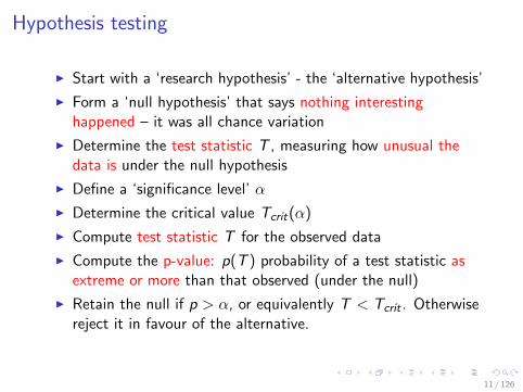
I Start with a ‘research hypothesis’ - the ‘alternative hypothesis’
I Form a ‘null hypothesis’ that says nothing interestinghappened – it was all chance variation
I Determine the test statistic T , measuring how unusual thedata is under the null hypothesis
I Define a ‘significance level’ α
I Determine the critical value Tcrit(α)
I Compute test statistic T for the observed data
I Compute the p-value: p(T ) probability of a test statistic asextreme or more than that observed (under the null)
I Retain the null if p > α, or equivalently T < Tcrit . Otherwisereject it in favour of the alternative.
11 / 126

Section 2
The Z test
12 / 126
Subsection 1
The simple Z test
13 / 126

The simple Z test
For n data points Xi
I If the mean of the data can be treated as Normal,
I And our null hypothesis is X = µ for known µ...
I And we know the standard deviation σ...
I Then we compute the test statistic Z = (X − µ)/σ...
I Under the null, Z ∼ N(0, 1)
So the Z test computes
I p(Z ′ ≥ Z ) (one tailed)
I p(|Z ′| ≥ |Z |) (two tailed)
I where Z ′ is from the null
14 / 126

Important properties of the Normal distribution
If X is normal then aX + b is normalIf X and Y are normal and independent, then X + Y is normal.Specifically, Z = X + Y ∼ N(µX + µY , σ
2X + σ2
Y ).
Meaning that we add the variance, regardless of whether we add Xand Y !More generally, if X and Y are correlated,
var(X + Y ) = σ2X + σ2
Y + 2ρσXσY
15 / 126

Important properties of the Normal distribution
If X is normal then aX + b is normalIf X and Y are normal and independent, then X + Y is normal.Specifically, Z = X + Y ∼ N(µX + µY , σ
2X + σ2
Y ).
Meaning that we add the variance, regardless of whether we add Xand Y !
More generally, if X and Y are correlated,
var(X + Y ) = σ2X + σ2
Y + 2ρσXσY
15 / 126

Important properties of the Normal distribution
If X is normal then aX + b is normalIf X and Y are normal and independent, then X + Y is normal.Specifically, Z = X + Y ∼ N(µX + µY , σ
2X + σ2
Y ).
Meaning that we add the variance, regardless of whether we add Xand Y !More generally, if X and Y are correlated,
var(X + Y ) = σ2X + σ2
Y + 2ρσXσY
15 / 126

Law of large numbers
Let X1, . . . ,Xn be independent samples from a distribution withmean µ and variance σ2. Then
X :=1
n(X1 + . . .+ Xn)
converges to µ as n→∞.
I ‘Estimate’ of µ: X
I Variance of the estimator: var(X ) = σ2/n
I ‘standard error’ SE : SD(X ) = σ/√n
So Z := X−µσ/√
nis ‘standardized’ to have mean 0 and s.d. 1.
16 / 126

Takeaway message:
I You can assume that the mean of1 a distribution is normal
I ... if n (sample size) is big enough
I IT DOESNT MATTER if the data you sampled were normallydistributed.
I The mean still has to be normally distributed
I How big is ‘big enough’? It depends on the distribution!
1: There are some special distributions that don’t obey the law of large numbers. These have infinite variance.
17 / 126

Z test example
I British birthweights haveMean 3426g and SD 538gfrom a large sample
I Australian birthweightssampled (1 day)
I Australians have mean 3276
I Null: birthweights have thesame mean
I Alternative: Australianbabies are smaller
18 / 126
Z test example
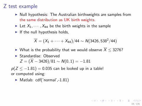
I Null hypothesis: The Australian birthweights are samples fromthe same distribution as UK birth weights.
I Let X1, · · · ,X44 be the birth weights in the sample
I If the null hypothesis holds,
X = (X1 + · · ·+ X44)/44 ∼ N(3426, 5382/44)
I What is the probability that we would observe X ≤ 3276?
I Standardise: ObservedZ = (X − 3426)/81 ∼ N(0, 1) = −1.81
p(Z ≤ −1.81) = 0.035 can be looked up in a table!or computed using:
I Matlab: cdf(’normal’,-1.81)
I R: pnorm(-1.81)
I Excel: (I’m not going to encourage this!)
I Wolfram Alpha, your phone, Google, etc!
19 / 126
Z test example
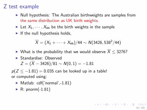
I Null hypothesis: The Australian birthweights are samples fromthe same distribution as UK birth weights.
I Let X1, · · · ,X44 be the birth weights in the sample
I If the null hypothesis holds,
X = (X1 + · · ·+ X44)/44 ∼ N(3426, 5382/44)
I What is the probability that we would observe X ≤ 3276?
I Standardise: ObservedZ = (X − 3426)/81 ∼ N(0, 1) = −1.81
p(Z ≤ −1.81) = 0.035 can be looked up in a table!or computed using:
I Matlab: cdf(’normal’,-1.81)
I R: pnorm(-1.81)
I Excel: (I’m not going to encourage this!)
I Wolfram Alpha, your phone, Google, etc!
19 / 126

Z test example
I Null hypothesis: The Australian birthweights are samples fromthe same distribution as UK birth weights.
I Let X1, · · · ,X44 be the birth weights in the sample
I If the null hypothesis holds,
X = (X1 + · · ·+ X44)/44 ∼ N(3426, 5382/44)
I What is the probability that we would observe X ≤ 3276?
I Standardise: ObservedZ = (X − 3426)/81 ∼ N(0, 1) = −1.81
p(Z ≤ −1.81) = 0.035 can be looked up in a table!or computed using:
I Matlab: cdf(’normal’,-1.81)
I R: pnorm(-1.81)
I Excel:
(I’m not going to encourage this!)
I Wolfram Alpha, your phone, Google, etc!
19 / 126

Z test example
I Null hypothesis: The Australian birthweights are samples fromthe same distribution as UK birth weights.
I Let X1, · · · ,X44 be the birth weights in the sample
I If the null hypothesis holds,
X = (X1 + · · ·+ X44)/44 ∼ N(3426, 5382/44)
I What is the probability that we would observe X ≤ 3276?
I Standardise: ObservedZ = (X − 3426)/81 ∼ N(0, 1) = −1.81
p(Z ≤ −1.81) = 0.035 can be looked up in a table!or computed using:
I Matlab: cdf(’normal’,-1.81)
I R: pnorm(-1.81)
I Excel: (I’m not going to encourage this!)
I Wolfram Alpha, your phone, Google, etc!
19 / 126

Z test example
I Null hypothesis: The Australian birthweights are samples fromthe same distribution as UK birth weights.
I Let X1, · · · ,X44 be the birth weights in the sample
I If the null hypothesis holds,
X = (X1 + · · ·+ X44)/44 ∼ N(3426, 5382/44)
I What is the probability that we would observe X ≤ 3276?
I Standardise: ObservedZ = (X − 3426)/81 ∼ N(0, 1) = −1.81
p(Z ≤ −1.81) = 0.035 can be looked up in a table!or computed using:
I Matlab: cdf(’normal’,-1.81)
I R: pnorm(-1.81)
I Excel: (I’m not going to encourage this!)
I Wolfram Alpha, your phone, Google, etc!19 / 126

Tails of the Normal Distribution
20 / 126
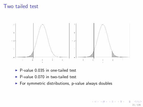
Two tailed test
I P-value 0.035 in one-tailed test
I P-value 0.070 in two-tailed test
I For symmetric distributions, p-value always doubles
21 / 126
Does it matter how many tails?
I Not really... Just make sure you’re clear on why.
I Switching from two-tailed to one-tailed can make anon-significant result significant.
I Hypothesis testing is in the business of being conservative...
I You should therefore have to justify a one-tailed choice.
I Previously, before we looked at the data, did we expectAustralian babies to be smaller? Would we not have beeninterested if they were bigger?
I If that was interesting too, we need a two-tailed test.
22 / 126
Requiem on errors: Power and alternative hypotheses
−2 −1 0 1 2 3 4
0.0
0.2
0.4
Null Distribution
x
−−> rejection region
1.644854
α
−2 −1 0 1 2 3 4
0.0
0.2
0.4
Alternative Distribution
x
−−> rejection region
1.644854
Power
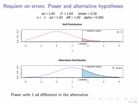
se = 1.00 z* = 1.64 power = 0.26 n = 1 sd = 1.00 diff = 1.00 alpha = 0.050
Power with 1 sd difference in the alternative
23 / 126

Requiem on errors: Power and alternative hypotheses
−2 −1 0 1 2 3 4
0.0
0.2
0.4
Null Distribution
x
−−> rejection region
1.644854
α
−2 −1 0 1 2 3 4
0.0
0.2
0.4
Alternative Distribution
x
−−> rejection region
1.644854
Power
se = 1.00 z* = 1.64 power = 0.991 n = 1 sd = 1.00 diff = 4.00 alpha = 0.050
Power with 4 sd difference in the alternative
24 / 126

Subsection 2
The Z test for proportions
25 / 126

Testing the number of successes
I Test: observe X successes from n trials
I H0: X/n = p, we are testing the probability of a success
I Let Ci ∼ Bern(p)
I i.e. Bernoilli with p=success probability,
I X =∑n
i=1 Ci ∼ Binomial(n, p) is the number of successes
I Can compute p(X ≤ x ; n, p) (too few successes) andp(X ≥ x ; n, p) (too many successes) explicitly for moderate n
I But do we need to?
26 / 126

Normal approximation to the Binomial
I If X ∼ Bin(n, p) then X is approximately distributed asN(µ, σ2) when n is large
I With µ = np and σ2 = np(1− p)
I What is large? Rule of thumb: µ ≥ 3σ
I What is meant by approximately? P(a < X < b) is close toP(a < µ+ σZ < b) for Z ∼ N(0, 1)
27 / 126

Binom(n=3,p=0.5)
28 / 126

Binom(n=10,p=0.5)
29 / 126

Binom(n=25,p=0.5)
30 / 126

Binom(n=100,p=0.5)
31 / 126

Binom(n=3,p=0.1)
32 / 126
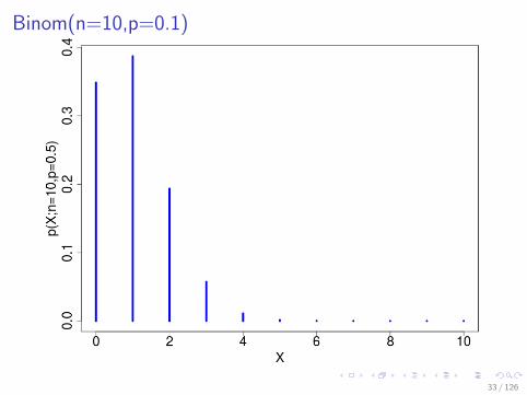
Binom(n=10,p=0.1)
33 / 126
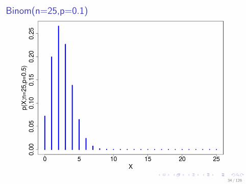
Binom(n=25,p=0.1)
34 / 126

Binom(n=100,p=0.1)
35 / 126

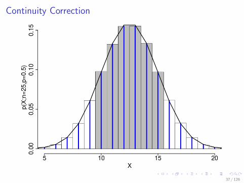
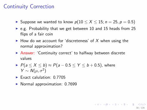
Continuity Correction
I Suppose we wanted to know p(10 ≤ X ≤ 15; n = 25, p = 0.5)
I e.g. Probability that we get between 10 and 15 heads from 25flips of a fair coin
I How do we account for ‘discreteness’ of X when using thenormal approximation?
I Answer: ‘Continuity correct’ to halfway between discretevalues
I P(a ≤ X ≤ b) ≈ P(a− 0.5 ≤ Y ≤ b + 0.5), whereY ∼ N(µ, σ2)
I Exact calulation: 0.7705
I Normal approximation: 0.7699
I Relative error: = (exact-normal)/exact = 0.0008
36 / 126
Continuity Correction
37 / 126

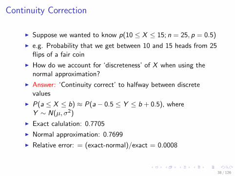
Continuity Correction
I Suppose we wanted to know p(10 ≤ X ≤ 15; n = 25, p = 0.5)
I e.g. Probability that we get between 10 and 15 heads from 25flips of a fair coin
I How do we account for ‘discreteness’ of X when using thenormal approximation?
I Answer: ‘Continuity correct’ to halfway between discretevalues
I P(a ≤ X ≤ b) ≈ P(a− 0.5 ≤ Y ≤ b + 0.5), whereY ∼ N(µ, σ2)
I Exact calulation: 0.7705
I Normal approximation: 0.7699
I Relative error: = (exact-normal)/exact = 0.0008
38 / 126

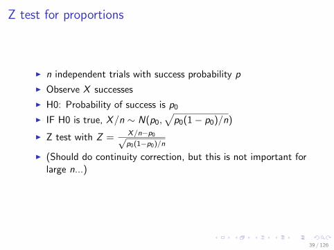
Z test for proportions
I n independent trials with success probability p
I Observe X successes
I H0: Probability of success is p0
I IF H0 is true, X/n ∼ N(p0,√
p0(1− p0)/n)
I Z test with Z = X/n−p0√p0(1−p0)/n
I (Should do continuity correction, but this is not important forlarge n...)
39 / 126
Z test for proportions
I n independent trials with success probability p
I Observe X successes
I H0: Probability of success is p0
I IF H0 is true, X/n ∼ N(p0,√
p0(1− p0)/n)
I Z test with Z = X/n−p0√p0(1−p0)/n
I (Should do continuity correction, but this is not important forlarge n...)
39 / 126

Example: ESP
I Charles Tart (1970s): 7500 (500x15) attempts on ’Aquariusmachine’
I Subjects predict which of four lights will come on
I Signal tells them if they were right.
I 7500 attempts. Expect 7500/4=1875 right.
I Actually observed 2006 correct guesses. Could it be purely bychance?
40 / 126

Example: ESP
I H0: Probability of success p = 0.25
I H1: Probability of success p > 0.25
I Significance level 0.01, meaning Zcrit = 2.3
I X = 2006/7500 = 0.26747, σ =√
0.25× 0.75/7500 = 0.005
Z =0.26747− 0.25
0.005= 3.49
I Comfortably above critical value. p = 0.0002
41 / 126

ESP conclusions
Did the subjects do so well purely by chance?
I Almost certainly not. Under the null this would happen in oneexperiment out of 5000.
I Should we conclude that some of the subjects had the powerto see into the future and predict which light would come on?
I Can you think of other alternatives?
I In fact, there was a problem with the machine which madethe order of the lights be not independent.
Conclusion: You have to be careful in interpreting the results ofstatistical tests. Just because you can show it didn’t happen ‘bychance’ doesnt mean your favourite alternative holds.
42 / 126
Subsection 3
The Z test for the difference between means
43 / 126

Z test for difference between means
I Observations from two different populations.
I Means from both are normally distributed.
I SDs are known: σ1 and σ2
I Unknown means µ1 and µ2
I Observe mean X 1 from n1 pop 1 samples and mean X 2 fromn2 pop 2 samples
I Test H0 : µ1 = µ2
I If H0 is true, X1 − X2 ∼ N(0, σ2)
I with σ =√σ2
1/n1 + σ22/n2
I Test statistic Z = (X 1 − X 2)/σ
44 / 126

Example: Do tall men get picked first?Heights of K Husbands, by age of marriage
Age of marriageearly (< 30) late (≥ 30)
number 160 35mean height (mm) 1735 1716
I Suppose we know that the standard deviation of height is70mm
I σ =√σ2
1/n1 + σ22/n2 = 13.1
Z =1735− 1716
13.1= 1.45
I One tailed p-value 0.0735
I Conclusion: Insufficient evidence to reject the nullI Weitzman & Conley: “From Assortative to Ashortative
Coupling: Men’s Height, Height Heterogamy, andRelationship Dynamics in the United States”: Short men tendto get married later ... but to stay married longer...
45 / 126

Example: Do tall men get picked first?Heights of K Husbands, by age of marriage
Age of marriageearly (< 30) late (≥ 30)
number 160 35mean height (mm) 1735 1716
I Suppose we know that the standard deviation of height is70mm
I σ =√σ2
1/n1 + σ22/n2 = 13.1
Z =1735− 1716
13.1= 1.45
I One tailed p-value 0.0735I Conclusion: Insufficient evidence to reject the null
I Weitzman & Conley: “From Assortative to AshortativeCoupling: Men’s Height, Height Heterogamy, andRelationship Dynamics in the United States”: Short men tendto get married later ... but to stay married longer...
45 / 126

Example: Do tall men get picked first?Heights of K Husbands, by age of marriage
Age of marriageearly (< 30) late (≥ 30)
number 160 35mean height (mm) 1735 1716
I Suppose we know that the standard deviation of height is70mm
I σ =√σ2
1/n1 + σ22/n2 = 13.1
Z =1735− 1716
13.1= 1.45
I One tailed p-value 0.0735I Conclusion: Insufficient evidence to reject the nullI Weitzman & Conley: “From Assortative to Ashortative
Coupling: Men’s Height, Height Heterogamy, andRelationship Dynamics in the United States”: Short men tendto get married later ... but to stay married longer...
45 / 126
Subsection 4
Z test for the difference between proportions
46 / 126

Z test for difference between proportions
I Observations from two different kinds of trials.
I Probabilities of success are p1 and p2
I Test H0 : p1 = p2
I Observe X1 successes from n1 trials from pop 1
I Observe X2 successes from n2 trials from pop 2
I Standardized test statistic:
Z =p̂1 − p̂2√
p̂(1− p̂)(
1n1
+ 1n2
)I with p̂1 = X1/n1, p̂2 = X2/n2 and p̂ = (X1 + X2)/(n1 + n2)
47 / 126

Example: Circumcision and AIDS
Study in Uganda: 70 circumcised men, 54 controls.
circum. non-circum.
n 70 54infected 11 4
I p̂1 = 11/70 = 0.157
I p̂2 = 4/54 = 0.121
I σ =√
0.121× 0.157(
170 + 1
54
)= 0.059
I Z = 0.157−0.1210.059 = 1.41
I One tailed p-value 0.08
I Conclusion: Insufficient evidence to reject the null
48 / 126

Section 3
The t test
49 / 126

Subsection 1
The simple t test
50 / 126

Example: Kidney Dialysis
I Phosphate measure in blood of dialysis patients on sixsuccessive visits. Known to vary approximately according tonormal distribution.
I One patient had the following measures in mg/dl:
5.6, 5.1, 4.6, 4.8, 5.7, 6.4
I Suppose 4.0 or below is a dangerous level.
I Test at the 0.01 level whether the level might be that low.
I X = 5.4mg/dl (empirical mean)
I s = 0.67mg/dl (empirical standard deviation)
51 / 126
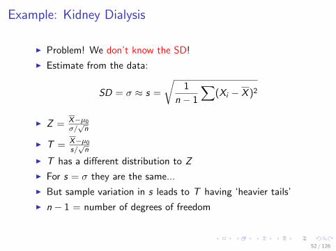
Example: Kidney Dialysis
I Problem! We don’t know the SD!
I Estimate from the data:
SD = σ ≈ s =
√1
n − 1
∑(Xi − X )2
I Z = X−µ0
σ/√
n
I T = X−µ0
s/√
n
I T has a different distribution to Z
I For s = σ they are the same...
I But sample variation in s leads to T having ‘heavier tails’
I n − 1 = number of degrees of freedom
52 / 126
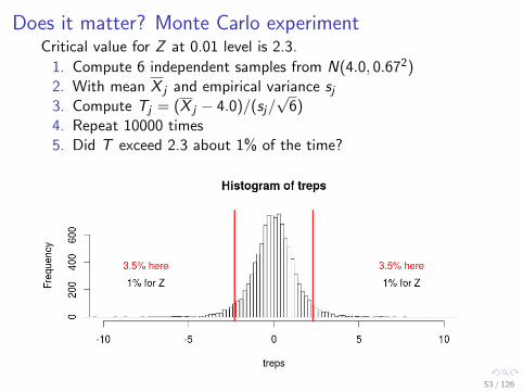
Does it matter? Monte Carlo experimentCritical value for Z at 0.01 level is 2.3.
1. Compute 6 independent samples from N(4.0, 0.672)2. With mean X j and empirical variance sj
3. Compute Tj = (X j − 4.0)/(sj/√
6)4. Repeat 10000 times5. Did T exceed 2.3 about 1% of the time?
53 / 126

The t test
I Suppose 4.0 or below is a dangerous level.
I Want a 1% chance of failing to recognise that the level is low
I H0: Average phosphate level = 4.0 mg/dl
I H1: Average phosphate level > 4.0 mg/dl
T =X − µs/√n
=5.4− 4.0
0.67/√
6= 5.12
I Matlab: tinv(0.99,5)=3.36
I i.e. the critical value is 3.36
I Observed T is bigger - reject H0
54 / 126
The simple t test (Student’s t test)
For n data points Xi
I If the mean of the data can be treated as Normal ...
I And our null hypothesis is X = µ for known µ...
I When we estimate the standard deviation σ using s...
I We compute the standard error SE = s/√n
I We compute the test statistic T = (X − µ)/SE ...
I Under the null, T ∼ t(0, 1, df = n − 1)
So the t test (also) computes p(T ′ ≥ T ) (one tailed)Or p(|T ′| ≥ |T |) (two tailed)Important note: more generally, df = n − p with p unknownparameters
55 / 126

Z test example
I British birthweights haveMean 3426g and SD 538gfrom a large sample
I Australian birthweightssampled (1 day)
I Australians have mean 3276
I Null: birthweights have thesame mean
I Alternative: Australianbabies are smaller
56 / 126

t test exampleNow imagine that we were not provided with the standarddeviation of the British sample.
I Null hypothesis: The Australian birthweights are samples fromthe same distribution as UK birth weights.
I With one unknown parameter: σ
I If the null hypothesis holds,
X = (X1 + · · ·+ X44)/44 ∼ N(3426, SE 2)
with SE = SD(Xi )/√
44 = 84.5
I What is the probability that we would observe X ≤ 3276?
I Standardise: Observedt = (x − 3426)/84.5 ∼ t(df = 44− 1) = −1.64
p(t ≤ −1.64) = 0.054. Bigger than before:
I Tails of t(n) larger than tails of N(0, 1)
I Because of uncertainty in σ̂57 / 126

Tails of the student t-distribution
Standard Errors from Zero
−4 −2 0 2 4
−2.571 2.571
95%
−1.960 1.960
Normalt, df=5
5 degrees of freedom
58 / 126

Tails of the student t-distribution
Standard Errors from Zero
−4 −2 0 2 4
−2.042 2.042
95%
−1.960 1.960
Normalt, df=30
30 degrees of freedom
59 / 126
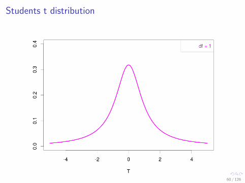
Students t distribution
60 / 126
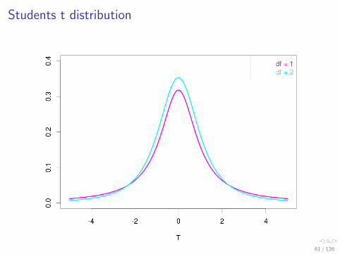
Students t distribution
61 / 126
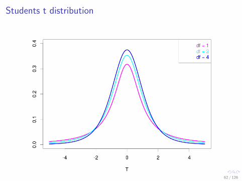
Students t distribution
62 / 126

Students t distribution
63 / 126
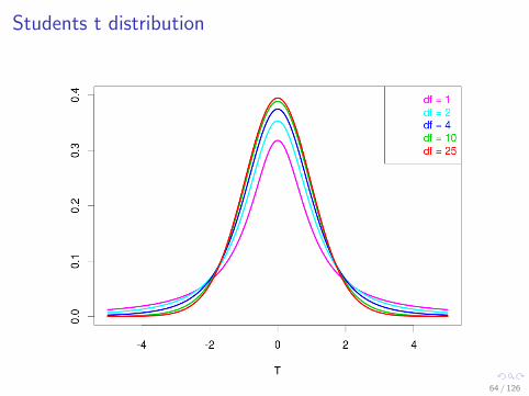
Students t distribution
64 / 126
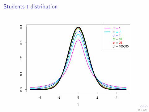
Students t distribution
65 / 126
Quiz time!
Let tα(d) be the α quantile of the Student T distribution with dd.f. i.e. the probability of t < α.
I t0.95(2) > t0.95(3)?
I true
I tα(100) is a little smaller than Zα?
I false - it can be very different for small α
I 1% of the measurements of average phosphate will be within2.3 s.d. of 4.0?
I false - that is only true for Z
66 / 126
Subsection 2
The Matched sample t test
67 / 126

Example - Schizophrenia
I 15 healthy, 15 Schizophreniasufferers
I Measure hippocampus volume
I schizophrenic:1.27,1.63,1.47,1.39,1.93,1.26,1.71,1.67,1.28,1.85,1.02,1.34,2.02,1.59,1.97
I healthy:1.94,1.44,1.56,1.58,2.06,1.66,1.75,1.77,1.78,1.92,1.25,1.93,2.04,1.62,2.08
I Test for equality of means at 0.05level.
I Dont know SD.
Unaff. Schiz.
Mean 1.76 1.56SD 0.24 0.30
68 / 126

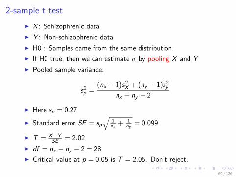
2-sample t test
I X : Schizophrenic data
I Y : Non-schizophrenic data
I H0 : Samples came from the same distribution.
I If H0 true, then we can estimate σ by pooling X and Y
I Pooled sample variance:
s2p =
(nx − 1)s2X + (ny − 1)s2
y
nx + ny − 2
I Here sp = 0.27
I Standard error SE = sp
√1
nx+ 1
ny= 0.099
I T = X−YSE = 2.02
I df = nx + ny − 2 = 28
I Critical value at p = 0.05 is T = 2.05. Don’t reject.
69 / 126
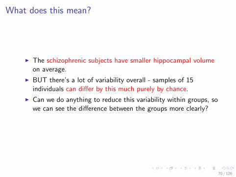
What does this mean?
I The schizophrenic subjects have smaller hippocampal volumeon average.
I BUT there’s a lot of variability overall - samples of 15individuals can differ by this much purely by chance.
I Can we do anything to reduce this variability within groups, sowe can see the difference between the groups more clearly?
70 / 126

Subsection 3
Matched sample t test
71 / 126

Matched case-control study
I Idea: Experiment and control group are in matched pairs,chosen to be similar in ways likely to affect what we’remeasuring.
I Why?
I A lot of the variability will disappear (we hope) from thedifference, since the matched pairs will vary together.
I Shared variance cancels out!
72 / 126
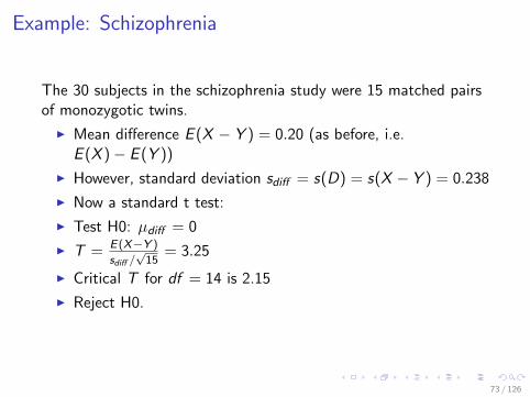
Example: Schizophrenia
The 30 subjects in the schizophrenia study were 15 matched pairsof monozygotic twins.
I Mean difference E (X − Y ) = 0.20 (as before, i.e.E (X )− E (Y ))
I However, standard deviation sdiff = s(D) = s(X −Y ) = 0.238
I Now a standard t test:
I Test H0: µdiff = 0
I T = E(X−Y )
sdiff /√
15= 3.25
I Critical T for df = 14 is 2.15
I Reject H0.
73 / 126

Section 4
The χ2 test
74 / 126

Subsection 1
The χ2 test
75 / 126

Example: suicides by birth month
Salib and Cortina-Borja ex-amined death certificates of26,886 suicides in England andWales. Tabulated by month ofbirth.Does spring birthday predis-pose to suicide?
Month Female Male Total
Jan 527 1774 2301Feb 435 1639 2074Mar 454 1939 2393Apr 493 1777 2270May 535 1969 2504Jun 515 1739 2254Jul 490 1872 2362Aug 489 1833 2322Sep 476 1624 2100Oct 474 1661 2135Nov 442 1568 2010Dec 471 1690 2161
76 / 126
Example: suicides by birth month
I Null hypothesis: Suicides are equally likely to have been bornany day of the year. The probability of having been born in agiven month is proportional to the number of days in themonth.
I Test the null hypothesis at the 0.01 level.
I One approach: Divide into two groups, and use the Z test
I If we define spring as March–June, there are 122 days
I Under H0 P(spring birthday) = 122/365.25 = 0.34
I Observed number spring = 9421
I Expected number spring = 0.334× 26886 = 8980
I Standard Error =√
0.334× 0.666× 26886 = 77.3
I Z = 9421−898077.3 = 5.71
I Critical value Zcrit = 2.58
I p-value ≈ 10−8
77 / 126

Example: suicides by birth month
I Problem: We cheated!
I We used the largest choice of months
I Was that our hypothesis before we saw the data?
I No. We might have instead wondered if there were anymonths that were unusual
I Can we test all deviations simultaneously?
78 / 126

The χ2 test
I Test statistic that measures deviations in all k categoriessimultaneously.
I χ2 =∑ (observedi−predicted)2
expected
I Zi = observedi−predictedstandard error
I χ2(k) =∑
k−1 Z2i where Zi are independent
I Mathematical fact: If the number of observations is large thenthis chi-squared statistic has a certain distribution, called theχ2 distribution.
I How large is large? Rule of thumb: At least 5 expected ineach cell of the table.
I This distribution also has a ‘degrees of freedom’ parameter
I General rule: df = Num. data pts - parameters estimated - 1
I So here: df = cells - parameters estimated - 1
79 / 126
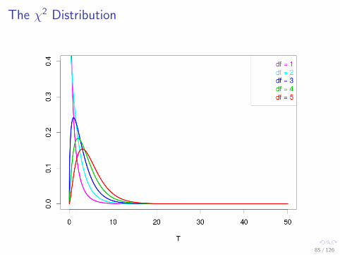
Calculating with χ2
I χ2 with d degrees of freedom has mean d and variance 2d .
I It has a density proportional to
xd/2−1e−x/2
I We will not use this formula, instead using the computer (asusual!)
80 / 126
The χ2 Distribution
81 / 126

The χ2 Distribution
82 / 126
The χ2 Distribution
83 / 126

The χ2 Distribution
84 / 126
The χ2 Distribution
85 / 126

The χ2 Distribution
86 / 126

The χ2 Distribution
87 / 126
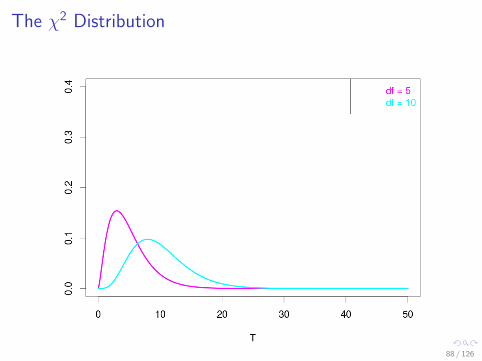
The χ2 Distribution
88 / 126

The χ2 Distribution
89 / 126

The χ2 Distribution
90 / 126
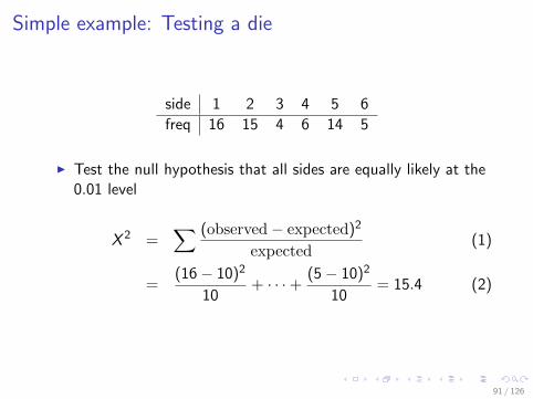
Simple example: Testing a die
side 1 2 3 4 5 6
freq 16 15 4 6 14 5
I Test the null hypothesis that all sides are equally likely at the0.01 level
X 2 =∑ (observed− expected)2
expected(1)
=(16− 10)2
10+ · · ·+ (5− 10)2
10= 15.4 (2)
91 / 126
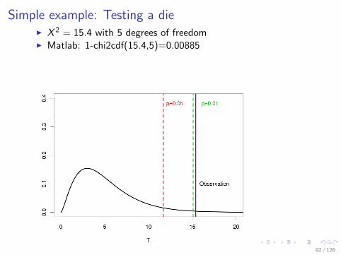
Simple example: Testing a dieI X 2 = 15.4 with 5 degrees of freedomI Matlab: 1-chi2cdf(15.4,5)=0.00885
I Reject at the 0.01 level
92 / 126

Simple example: Testing a dieI X 2 = 15.4 with 5 degrees of freedomI Matlab: 1-chi2cdf(15.4,5)=0.00885I Reject at the 0.01 level
92 / 126

Example: suicides by birth month
Salib and Cortina-Borja ex-amined death certificates of26,886 suicides in England andWales. Tabulated by month ofbirth.Does spring birthday predis-pose to suicide?
Month Female Male Total
Jan 527 1774 2301Feb 435 1639 2074Mar 454 1939 2393Apr 493 1777 2270May 535 1969 2504Jun 515 1739 2254Jul 490 1872 2362Aug 489 1833 2322Sep 476 1624 2100Oct 474 1661 2135Nov 442 1568 2010Dec 471 1690 2161
93 / 126
Suicides by birth month
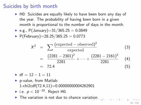
I H0: Suicides are equally likely to have been born any day ofthe year. The probability of having been born in a givenmonth is proportional to the number of days in the month.
I e.g., P(January)=31/365.25 = 0.0849
I P(February)=28.25/365.25 = 0.0773
X 2 =∑ (expected− observed)2
expected(3)
=(2281− 2301)2
2281+ · · ·+ (2281− 2161)2
2281(4)
= 72.4 (5)
I df = 12− 1 = 11
I p-value, from Matlab:1-chi2cdf(72.4,11)=0.00000000004262901
I i.e. p < 10−10. Reject H0.
I The variation is not due to chance variation.94 / 126

Suicides by birth month
I Looking at just the data for females:
X 2 =(492− 527)2
492+ · · ·+ (492− 471)2
492(6)
= 17.4 (7)
I Matlab: chi2inv(.95,11)=19.68
I We do not reject H0 at the 5% level....
I “The difference in frequency of suicides by birth monthamong women is NOT statistically significant. It could beexplained by chance variation.”
95 / 126
Section 5
Non-parametric tests
96 / 126

Subsection 1
Why we need non-parametric tests
97 / 126
An experiment
I “If a newborn infant is held under his arms and his bare feetare permitted to touch a flat surface, he will performwell-coordinated walking movements similar to those of anadult... Normally, the walking and pacing reflexes disappearby about 8 weeks.”
I Observation: If the infant exercises this reflex, it does notdisappear.
I Hypothesis: Maintaining this reflex will help children learn towalk earlier.
98 / 126

How do we test this hypothesis?
I Idea: Do weekly exercises with a newborn. See when he/shestarts walking.
I Result: 10 months.
I Problem: Is that long or short?
I New Idea: Do weekly exercises with a newborn. Don’t doweekly exercises with another newborn. See which one startswalking first
I Result: mean with exercise 10.1 months
I without exercise 11.7 months
I Problem: Newborns don’t all start walking at the same age,regardless of exercise.
99 / 126
t test for walking data
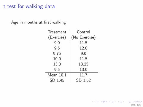
Age in months at first walking
Treatment Control(Exercise) (No Exercise)
9.0 11.59.5 12.0
9.75 9.010.0 11.513.0 13.259.5 13.0
Mean 10.1 11.7SD 1.45 SD 1.52
100 / 126
t test for walking data
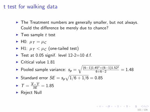
I The Treatment numbers are generally smaller, but not always.Could the difference be merely due to chance?
I Two sample t test
I H0: µT = µC
I H1: µT < µC (one-tailed test)
I Test at 0.05 signif. level 12-2=10 d.f.
I Critical value 1.81
I Pooled sample variance: sp =√
(6−1)1.452+(6−1)1.522
6+6−2 = 1.48
I Standard error SE = sp
√1/6 + 1/6 = 0.85
I T = X−YSE = 1.85
I Reject Null
101 / 126

What if the distribution isn’t Normal?
I Under the null...
I A bimodal distribution?
I Mean of 6 samples will not be Normal!
102 / 126
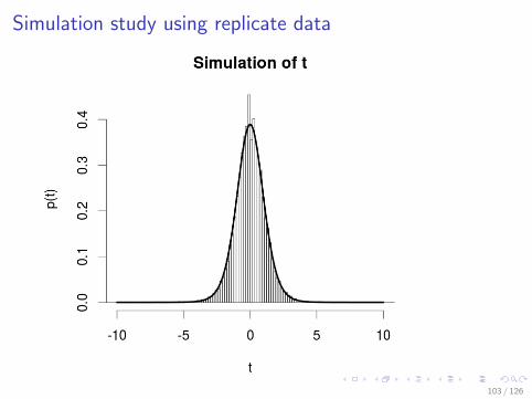
Simulation study using replicate data
103 / 126

Simulation study using replicate data
104 / 126

Nonparametric tests
I Idea: Come up with test statistics whose significance leveldoesn’t depend on the distribution that the data came from.
I Advantage: We reject with the right probability if the nullhypothesis is true.
I Drawback: We lose power. That is, we need a larger sampleto reject the null if its false.
I We focus on two tests that the median of two distributions isequal
I They are varyingly sensitive to other differences in distribution
105 / 126

Subsection 2
Mann-Whitney U test
106 / 126

Mann-Whitney U test
Also called the Wilcoxon two sample Rank-sum test
I We have samples X1, · · · ,Xnx and Y1, · · · ,Yny with unknowndistributions.
I H0: medians are the same.
I H1 :mx > my (one-tailed) or mx 6= my (two-tailed)
107 / 126
Mann-Whitney calculation
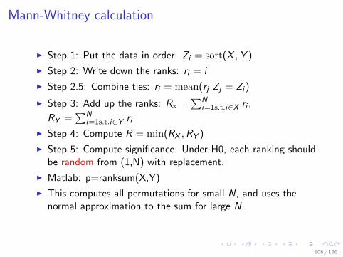
I Step 1: Put the data in order: Zi = sort(X ,Y )
I Step 2: Write down the ranks: ri = i
I Step 2.5: Combine ties: ri = mean(rj |Zj = Zi )
I Step 3: Add up the ranks: Rx =∑N
i=1s.t.i∈X ri ,
RY =∑N
i=1s.t.i∈Y riI Step 4: Compute R = min(RX ,RY )
I Step 5: Compute significance. Under H0, each ranking shouldbe random from (1,N) with replacement.
I Matlab: p=ranksum(X,Y)
I This computes all permutations for small N, and uses thenormal approximation to the sum for large N
108 / 126

Computation for walking babies
9.0 9.0 9.5 9.5 9.75 10.0 11.5 11.5 12 13.0 13.0 13.251.5 1.5 3.5 3.5 5 6 7.5 7.5 9 10.5 10.5 12
I RX = 30, RY = 48
I R = RX = 30 since X and Y have the same size
I p=ranksum(X,Y,’tail’,’left’) = 0.085 (recent matlab versionsonly!)
I p=ranksum(X,Y)/2 = 0.085 (old versions only implementtwo-tailed test)
I Retain the null hypothesis
109 / 126

Subsection 3
Paired value tests
110 / 126

The sign test
I We have paired samples X1,Y1, · · · ,Xn,Yn
I Work only with Ii = I(Xi − Yi > 0), i.e. 1 if Xi > Yi , 0otherwise.
I H0: S =∑
i Ii is a Binomial RV with success probabilityp = 0.5
I H1: p > 0.5
I Matlab: binocdf(S , n, 0.5) (left tail)
I Matlab: binocdf(n − S , n, 0.5) (right tail)
I Matlab: 2 min(binocdf(S , n, 0.5),binocdf(n − S , n, 0.5))(two-tailed)
111 / 126
Example: Schizophrenia
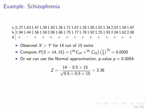
s. 1.27 1.63 1.47 1.39 1.93 1.26 1.71 1.67 1.28 1.85 1.02 1.34 2.02 1.59 1.97h. 1.94 1.44 1.56 1.58 2.06 1.66 1.75 1.77 1.78 1.92 1.25 1.93 2.04 1.62 2.08d. + - + + + + + + + + + + + + +
I Observed X > Y for 14 out of 15 twins
I Compute P(S = 14, 15) = (15C14 +15 C15)(
12
)15= 0.0005
I Or we can use the Normal approximation, p-value p = 0.0004:
Z =14− 0.5× 15√0.5× 0.5× 15
= 3.36
112 / 126

Wilcoxon one sample sign-rank test
I Idea: It makes sense to consider, not just if X > Y , butwhether this happens for big or small numbers.
I It might be that there are equal numbers of + and −differences, but the + are bigger
I Step 1: list differences ordered by absolute value
I Step 2: Calculate W = min(∑
i :X>Y (ri ),∑
i :X<Y (ri ))
I Step 3: Compare W to the distribution that would be givenunder the null, that the ranks are unrelated to the signs
I For small n this means enumerating all options (enumerationis not fun)
113 / 126

Wilcoxon one sample sign-rank test
I For n ≈ 10 or more, Z = W−µWσW
∼ N(0, 1), and a Z test canbe used,
I Where
µW =1
2+
n(n + 1)
4
and
σW =
√n(n + 1)(2n + 1)
24.
114 / 126

Example: Schizophrenia
s. 1.27 1.63 1.47 1.39 1.93 1.26 1.71 1.67 1.28 1.85 1.02 1.34 2.02 1.59 1.97h. 1.94 1.44 1.56 1.58 2.06 1.66 1.75 1.77 1.78 1.92 1.25 1.93 2.04 1.62 2.08d. 0.67 -0.19 0.09 0.19 0.13 0.40 0.04 0.10 0.50 0.07 0.23 0.59 0.02 0.03 0.11Leading to the sorted differences0.02 0.03 0.04 0.07 0.09 0.10 0.11 0.13 -0.19 0.19 0.23 0.40 0.50 0.59 0.67
1 2 3 4 5 6 7 8 9.5 9.5 11 12 13 14 15
I Sums: Rx = 110.5, RY = 9.5
I So R = 9.5
I µR = 0.5 + 15× 16/4 = 60.5
I σR =√
15× 16× (30 + 1)/24 = 17.6
I Z = (R − µR)/σR = −2.897
I So the p-value is 0.0019
115 / 126

Section 6
The menagerie of tests
116 / 126

But which test should I use???
I These are just a small subset of the possible tests availableI Many of them have different options:
I How did we make the data look like a Normal?I Parameters in model - leads to degrees of freedomI Tails of testI Pairing dataI etc
I How to decide?
117 / 126

Model assumptions
The key is to make appropriate assumptions
I Are your data independent and random samples from adefined population? (All tests considered here)
I Are you primarily testing for a difference in the location in thetwo distributions? (Z ,t,non-parametric tests)
I Or the variance of many random variables? (χ2)
I Is the underlying distribution normal? (Z test, t test, χ2 test)
I Or do we want to avoid assumptions about it, and test themedian? (Mann-Whitney, Wilcoxon)
I If so, do we want to test the whole distribution? (Wilcoxon)
I Are there unknown parameters? (t test, χ2 test)
Look up the specific assumptions when you use a test!
118 / 126

Z Test
H1 tests for a difference in the mean of two distributions.H0 makes the following assumptions:
I Independent random samples
I Mean is approx. normal
I Continuous variable (recall: continuity correction)
I Known variance
119 / 126
t Test
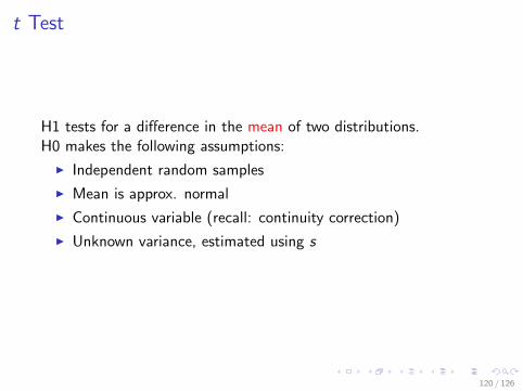
H1 tests for a difference in the mean of two distributions.H0 makes the following assumptions:
I Independent random samples
I Mean is approx. normal
I Continuous variable (recall: continuity correction)
I Unknown variance, estimated using s
120 / 126
χ2 Test
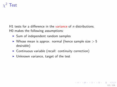
H1 tests for a difference in the variance of n distributions.H0 makes the following assumptions:
I Sum of independent random samples
I Whose mean is approx. normal (hence sample size > 5desirable)
I Continuous variable (recall: continuity correction)
I Unknown variance, target of the test
121 / 126

Sign Test
H1 tests for a difference in the median of two distributions.H0 makes the following assumptions:
I Independent random samples
122 / 126

Mann-Whitney U Test
H1 tests for a difference in the median of two distributions.H0 makes the following assumptions:
I Independent random samples
I Continuous variable (recall: tied value correction)
This is ‘just’ the unpaired Wilcoxon Test.
123 / 126

Wilcoxon Test
H1 tests for a difference in either the median of two paireddistributions.H0 makes the following assumptions:
I Independent random samples
I Continuous variable (recall: tied value correction)
I symmetric distribution of differences
124 / 126

Other tests you might encounter
We have looked at tests for the location of one or moredistributions. Other important cases are:
I F-test: Compares the variance of two distributions. Used inAnalysis of variance (ANOVA).
I Kolmogorov-Smirnov test: A non-parametric test for whethertwo distributions are the same, based on the maximumdeviation from the empirical cumulative density functions.
125 / 126

Conceptually different tests
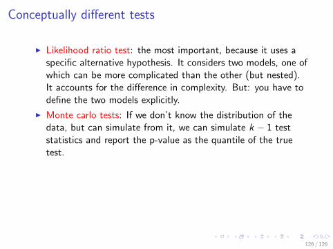
I Likelihood ratio test: the most important, because it uses aspecific alternative hypothesis. It considers two models, one ofwhich can be more complicated than the other (but nested).It accounts for the difference in complexity. But: you have todefine the two models explicitly.
I Monte carlo tests: If we don’t know the distribution of thedata, but can simulate from it, we can simulate k − 1 teststatistics and report the p-value as the quantile of the truetest.
I Bayesian tests: A very different paradigm, Bayesian testsusually ask whether a parameter estimate falls outside of somerange, given the data and some prior knowledge of theparameter.
126 / 126

Conceptually different tests
I Likelihood ratio test: the most important, because it uses aspecific alternative hypothesis. It considers two models, one ofwhich can be more complicated than the other (but nested).It accounts for the difference in complexity. But: you have todefine the two models explicitly.
I Monte carlo tests: If we don’t know the distribution of thedata, but can simulate from it, we can simulate k − 1 teststatistics and report the p-value as the quantile of the truetest.
I Bayesian tests: A very different paradigm, Bayesian testsusually ask whether a parameter estimate falls outside of somerange, given the data and some prior knowledge of theparameter.
126 / 126