joint inversion of seismic and electromagnetic data · joint inversion of seismic and...
TRANSCRIPT
I
Joint Inversion of Seismic and Electromagnetic Data
Application on two synthetic reservoirs
Carolina da Silva Carvalho
Thesis to obtain the Master of Science Degree in
Petroleum Engineering
Supervisor: Dr. Leonardo Azevedo Guerra Raposo Pereira
Examination Committee
Chairperson: Prof. Dr. Maria João Correia Colunas Pereira
Supervisor: Dr. Leonardo Azevedo Guerra Raposo Pereira
Members of the Committee: Eng. Dário Sergio Cersósimo
October 2015

II
This page was intentionally left blank.

III
Acknowledgements
The present thesis won’t be possible without the constant support of some amazing people that I’m very
thankful.
First, I like to thank for the support, help and patience of my advisor Dr. Leonardo Azevedo.
To my family for the encouragement through this last year and especially in the last few months, to make me
laugh and face the difficulties.
To my friends for their support, for the right words at the right time and especially for the moments to calm
down and look the things a different way.
At last, for my petroleum friends for the encouragement and the good vibe of our “office”.

IV
This page was intentionally left blank.

V
Abstract
Seismic inversion methodologies are well-established tools in the oil and gas industry to model the spatial extent
and characterize the petro-elastic subsurface properties of interest. Reservoir modeling and characterization
workflows tend nowadays to integrate all the available data, i.e. geological, well-log and geophysical data, within
the same geo-modeling workflow in order to decrease the uncertainty associated with the retrieved models.
In recent years, electromagnetic data become one important tool to determine possible subsurface hydrocarbon
accumulations with commercial potential, since it allows inferring the subsurface resistivity that is linked with
the pore-type fluid. Therefore, the integration of electromagnetic data, sensitive to fluid properties with seismic
data, sensitive to the elastic properties of the subsurface can provide more reliable subsurface models with lower
uncertainty.
In this thesis, we present an iterative geostatistical methodology that jointly invert controlled-source
electromagnetics and seismic data in order to obtain porosity, acoustic impedance and water saturation. The
convergence of the model is ensured by a genetic algorithm that acts as a global optimizer and, the perturbation
of the model parameters is performed recurring to stochastic sequential simulation and co-simulation. A pre-
calibrated rock physics model is used within the inversion loop to ensure the link of the elastic and petrophysical
domains.
This new implementation of the iterative geostatistical joint inversion methodology was implemented on two
different synthetic reservoir, Stanford VI-E and CERENA-I. The result for the petro-elastic properties were very
promising for both reservoirs.
Keywords: Geostatistical inversion, EM, seismic, joint inversion.

VI
This page was intentionally left blank

VII
Resumo
A utilização de metodologias de inversão geostatistica como ferramenta para modelar a extensão espacial e
caracterizar as propriedades petro-elásticas do substrato, são prática recorrente e bem estabelecida na indústria
petrolífera. Os processos de modelização e caracterização do reservatório tendem a integrar toda a informação
disponível, isto é, geológica, dados de poço e geofísica, no mesmo processo de inversão, de forma, a diminuir a
incerteza associadas aos modelos resultantes.
Nos últimos anos, os dados de electromagnetismo tornaram-se uma ferramenta importante na determinação de
possíveis acumulações de hidrocarbonetos, uma vez que permitem determinar a resistividade do subsolo, já que
esta depende dos fluídos presentes nos poros. Posto isto, a integração de dados de electromagnetismo, sensíveis
às propriedades dos fluídos, com dados sísmicos, sensíveis às propriedades elásticas do substrato, pode
proporcionar resultados mais realistas e com menos incerteza associada do substrato.
Na presente tese é utilzado um novo processo iterativo que inverte conjuntamente dados de CSEM e de sísmica
a fim de obter modelos petro-elásticos (porosidade, impedância acústica e saturação em água). A convergência
do modelo é assegurada por um algoritmo genético que atua como um optimizador global e, a perturbação do
modelo é realizada por simulação sequencial e co-simulação. Recorrendo a um modelo de rock physic pré-
calibrado é assegurada a ligação entre as caraterísticas eláticas e petrofísicas.
Esta nova metodologia iterativa de inversão conjunta geostatística foi implementada em dois reservatótios
sintéticos diferentes, StanfordVI-E e CERENA-I. Os resultados obtido para as propriedades petro-elásticas foram
promissores para ambos os reservatórios.
Palavras-chave: inversão geostatistica, EM, sismica, inversão conjunta.

VIII
This page was intentionally left blank
IX
Table of Contents
1. Introduction.................................................................................................................................................... 1
1.1. Motivation ............................................................................................................................................. 1
1.2. Objectives .............................................................................................................................................. 1
1.3. Structure of the thesis ........................................................................................................................... 2
2. Theory and Methods ...................................................................................................................................... 3
2.1. Seimic Inversion ..................................................................................................................................... 3
2.2. CSEM Inversion ...................................................................................................................................... 6
2.3. Joint Inversion ....................................................................................................................................... 9
3. Geostatistical Joint Inversion of seismic and EM ......................................................................................... 11
3.1. Direct sequential simulation and co-simulation with joint probability distributions .......................... 14
3.2. Siliciclastic synthetic reservoir – Stanford VI-E .................................................................................... 15
3.2.1. Dataset description ..................................................................................................................... 15
3.2.2. Results and Discussion ................................................................................................................ 19
3.2.2.1. Geostatistical seismic inversion .............................................................................................. 19
3.2.2.2. Geostatistical Joint Inversion – Scenario 1 ............................................................................. 21
3.2.2.3. Geostatistical Joint Inversion – Scenario 2 ............................................................................. 23
3.2.2.4. Geostatistical Joint Inversion – Scenario 3 ............................................................................. 25
3.2.2.5. Discussion of the results ......................................................................................................... 27
3.3. Carbonate synthetic reservoir – CERENA-I .......................................................................................... 32
3.3.1. Dataset description ..................................................................................................................... 32
3.3.2. Results and Discussion ................................................................................................................ 36
3.3.2.1. Geostatistical Seismic Inversion - GSI ..................................................................................... 36
3.3.2.2. Geostatistical Joint Inversion - Scenario 1 .............................................................................. 37
3.3.2.3. Geostatistical Joint Inversion - Scenario 2 .............................................................................. 39
3.3.2.4. Geostatistical Joint Inversion - Scenario 3 .............................................................................. 41
3.3.2.5. Discussion of the results ......................................................................................................... 43
4. Conclusions and further recommendations ................................................................................................. 47
5. References .................................................................................................................................................... 48

X
List of Figures
Figure 1 Diagram of the proposed algorithm in Caetano (2009) ............................................................................ 5 Figure 2 Process of creating "Best Correlation Cube" and "Best Acoustic Impedance cube" in Caetano (2009). .. 6 Figure 3 Marine EM concepts: Electric and magnetic field receivers are deployed on the seafloor to record
time-series measurements of the fields, which could be used to compute MT impedances. The seafloor
instruments also receive signals emitted by a CSEM transmitter (towed close to the seafloor) at ranges
of as much as about 10 km. The MT signals are associated with largely horizontal current flow in the
seafloor, and are sensitive only to large-scale structures. The CSEM signals involve both vertical and
horizontal current flow, which could be interrupted by oil and gas reservoirs to provide sensitivity to
these geologic structures even when they are quite thin in Constable (2010). ....................................... 8 Figure 4 Schematic representation of the geostatistical joint EM and seismic reflection data inversion workflow
in Azevedo and Soares (2014). ................................................................................................................ 12 Figure 5 Schematic representation of the interpolation used to during the selection of the best fit model per
iteration for the properties estimated during the iterative process of joint inversion of EM and seismic
data. ........................................................................................................................................................ 13 Figure 6 Stratigraphic model with layer 1 (left) and layer 2 (right) and facies (adapted from Lee and Mukerji
(2013)). .................................................................................................................................................... 16 Figure 7 Horizontal slice from real seismic model (z=96) and the respective histogram ..................................... 17 Figure 8 Horizontal slice from real resisitivity model (z=96) and the respective histogram. ................................ 17 Figure 9 Horizontal slice from real water saturation model (z=96) and the respective histogram. ..................... 18 Figure 10 Horizontal slice from real acoustic impedance model (z=96) and the respective histogram. .............. 19 Figure 11 Acoustic Impedance horizontal slice (z=96) from simulation 32 of the 6th iteration and respective
histogram resulting from GSI. ................................................................................................................. 20 Figure 12 Seismic horizontal slice (z=96) from the simulation 32 of the 6th iteration and respective histogram
resulting from GSI. .................................................................................................................................. 20 Figure 13 Horizontal slices (z=96) from scenario 1 seismic models demonstrating the evolution since the first
model simulated (left), best model from iteration 3 (middle) to the best model from iteration 6 (right).
................................................................................................................................................................ 21 Figure 14 Horizontal slices (z=96) from scenario 1 resistivity models demonstrating the evolution since the first
model simulated (left), best model from iteration 3 (middle) to the best model from iteration 6 (right).
................................................................................................................................................................ 21 Figure 15 Horizontal slices (z=96) from scenario 1 porosity models demonstrating the evolution since the first
model simulated (left), best model from iteration 3 (middle) to the best model from iteration 6 (right).
................................................................................................................................................................ 22 Figure 16 Horizontal slices (z=96) from scenario 1 water saturation models demonstrating the evolution since
the first model simulated (left), best model from iteration 3 (middle) to the best model from iteration
6 (right). .................................................................................................................................................. 22 Figure 17 Horizontal slices (z=96) from scenario 2 seismic models demonstrating the evolution since the first
model simulated (left), best model from iteration 3 (middle) to the best model from iteration 6 (right).
................................................................................................................................................................ 23 Figure 18 Horizontal slices (z=96) from scenario 2 resistivity models demonstrating the evolution since the first
model simulated (left), best model from iteration 3 (middle) to the best model from iteration 6 (right).
................................................................................................................................................................ 23 Figure 19 Horizontal slices (z=96) from scenario 2 porosity models demonstrating the evolution since the first
model simulated (left), best model from iteration 3 (middle) to the best model from iteration 6 (right).
................................................................................................................................................................ 24 Figure 20 Horizontal slices (z=96) from scenario 2 water saturation models demonstrating the evolution since
the first model simulated (left), best model from iteration 3 (middle) to the best model from iteration
6 (right). .................................................................................................................................................. 24

XI
Figure 21 Horizontal slices (z=96) from scenario 3 seismic models demonstrating the evolution since the first
model simulated (left), best model from iteration 3 (middle) to the best model from iteration 6 (right).
................................................................................................................................................................ 25 Figure 22 Horizontal slices (z=96) from scenario 3 resistivity models demonstrating the evolution since the first
model simulated (left), best model from iteration 3 (middle) to the best model from iteration 6 (right).
................................................................................................................................................................ 25 Figure 23 Horizontal slices (z=96) from scenario 3 porosity models demonstrating the evolution since the first
model simulated (left), best model from iteration 3 (middle) to the best model from iteration 6 (right).
................................................................................................................................................................ 26 Figure 24 Horizontal slices (z=96) from scenario 3 water saturation models demonstrating the evolution since
the first model simulated (left), best model from iteration 3 (middle) to the best model from iteration
6 (right). .................................................................................................................................................. 26 Figure 25 (a) Horizontal slices (z=96) from correlation coefficient cubes for seismic models resulting from the
last iteration of each scenario: scenario 1 (left), scenario 2(middle), scenario 3 (right). (b) Below, the
respective horizontal slice with the average mean calculated from the 32 simulation of the 6th
iteration. ................................................................................................................................................. 27 Figure 26 (a) Horizontal slices (z=96) from correlation coefficient cubes for resistivity models resulting from the
last iteration of each scenario: scenario 1 (left), scenario 2(middle), scenario 3 (right). (b) Below, the
respective horizontal slice with the average mean. ............................................................................... 28 Figure 27 Horizontal slices (z=96) from the average mean for porosity for each scenario: scenario 1(left),
scenario 2 (middle) and scenario 3 (right). ............................................................................................. 29 Figure 28 Horizontal slices (z=96) from the average mean for density for each scenario: scenario 1(left),
scenario 2 (middle) and scenario 3 (right). ............................................................................................. 29 Figure 29 Horizontal slices (z=96) from the average mean for acoustic impedance for each scenario: scenario
1(left), scenario 2 (middle) and scenario 3 (right). ................................................................................. 30 Figure 30 Horizontal slices (z=96) from the average mean for P-wave velocity for each scenario: scenario 1(left),
scenario 2 (middle) and scenario 3 (right). ............................................................................................. 30 Figure 31 Horizontal slices (z=96) from the average mean for water saturation for each scenario: scenario
1(left), scenario 2 (middle) and scenario 3 (right). ................................................................................. 31 Figure 32 Vertical slice from real seismic model and the respective histogram. ................................................. 33 Figure 33 Vertical slice from real resistivity model and the respective histogram. .............................................. 33 Figure 34 Vertical slice from real water saturation model and the respective histogram. .................................. 34 Figure 35 Vertical slice from real porosity model and the respective histogram. ................................................ 34 Figure 36 Vertical slice from real acoustic impedance model and the respective histogram. ............................. 35 Figure 37 Vertical slice from best seismic model resulting from the last iteration of GSI .................................... 36 Figure 38 Vertical slice from best acoustic impedance model resulting from the last iteration of GSI. ............... 37 Figure 39 Vertical slices from scenario 1 seismic models demonstrating the evolution since the first model
simulated (left), best model from iteration 3 (middle) to the best model from iteration 6 (right). ....... 37 Figure 40 Vertical slices from scenario 1 resistivity models demonstrating the evolution since the first model
simulated (left), best model from iteration 3 (middle) to the best model from iteration 6 (right). ....... 38 Figure 41 Vertical slices from scenario 1 porosity models demonstrating the evolution since the first model
simulated (left), best model from iteration 3 (middle) to the best model from iteration 6 (right). ....... 38 Figure 42 Vertical slices from scenario 1 water saturation models demonstrating the evolution since the first
model simulated (left), best model from iteration 3 (middle) to the best model from iteration 6 (right).
................................................................................................................................................................ 38 Figure 43 Vertical slices from scenario 2 seismic models demonstrating the evolution since the first model
simulated (left), best model from iteration 3 (middle) to the best model from iteration 6 (right). ....... 39 Figure 44 Vertical slices from scenario 2 resistivity models demonstrating the evolution since the first model
simulated (left), best model from iteration 3 (middle) to the best model from iteration 6 (right). ....... 39 Figure 45 Vertical slices from scenario 2 porosity models demonstrating the evolution since the first model
simulated (left), best model from iteration 3 (middle) to the best model from iteration 6 (right). ....... 40

XII
Figure 46 Vertical slices from scenario 2 water saturation models demonstrating the evolution since the first
model simulated (left), best model from iteration 3 (middle) to the best model from iteration 6 (right).
................................................................................................................................................................ 40 Figure 47 Vertical slices from scenario 3 seismic models demonstrating the evolution since the first model
simulated (left), best model from iteration 3 (middle) to the best model from iteration 6 (right). ....... 41 Figure 48 Vertical slices from scenario 3 resistivity models demonstrating the evolution since the first model
simulated (left), best model from iteration 3 (middle) to the best model from iteration 6 (right). ....... 41 Figure 49 Vertical slices from scenario 3 porosity models demonstrating the evolution since the first model
simulated (left), best model from iteration 3 (middle) to the best model from iteration 6 (right). ....... 42 Figure 50 Vertical slices from scenario 3 water saturation models demonstrating the evolution since the first
model simulated (left), best model from iteration 3 (middle) to the best model from iteration 6 (right).
................................................................................................................................................................ 42 Figure 51 (a) Vertical slices from correlation coefficient cubes for seismic models resulting from the last
iteration of each scenario: scenario 1 (left), scenario 2(middle), scenario 3 (right). (b) Below, the
respective vertical slice from the best model from the last iteration..................................................... 43 Figure 52 (a) Vertical slices from correlation coefficient cubes for resistivity models resulting from the last
iteration of each scenario: scenario 1 (left), scenario 2(middle), scenario 3 (right). (b) Below, the
respective vertical slice from the best model from the last iteration..................................................... 44 Figure 53 Vertical slices from the average mean for porosity for each scenario: scenario 1(left), scenario 2
(middle) and scenario 3 (right). ............................................................................................................... 44 Figure 54 Vertical slices from the average mean for density for each scenario: scenario 1(left), scenario 2
(middle) and scenario 3 (right). ............................................................................................................... 45 Figure 55 Vertical slices from the average mean for acoustic impedance for each scenario: scenario 1(left),
scenario 2 (middle) and scenario 3 (right). ............................................................................................. 45 Figure 56 Vertical slices from the average mean for P-wave velocity models for each scenario: scenario 1(left),
scenario 2 (middle) and scenario 3 (right). ............................................................................................. 45 Figure 57 Vertical slices from the average mean for water saturation models for each scenario: scenario 1(left),
scenario 2 (middle) and scenario 3 (right). ............................................................................................. 46

XIII
List of Tables
Tab. 1 Simplified rock physics model used to link the elastic and the petrophysical properties (adapted from
Lee and Mukerji (2013)). ............................................................................................................................ 16
Tab. 2 Fluid properties used in the iterative procedure for SVI-E reservoir (adapted from Lee and Mukerji
(2013)). ...................................................................................................................................................... 16
Tab. 3 Simplified rock physics model used to link the elastic and the petrophysical properties ( adapted from
Pinto (2014)). ............................................................................................................................................. 32
Tab. 4 Fluids properties used in the iterative process for Cerena-I ..................................................................... 32

XIV
This page was intentionally left blank

1
1. Introduction
Nowadays, the increasing complexity of oil and gas reservoirs with increasingly water depths, translating in
higher exploration and production costs, raises the need for new methodologies for better subsurface Earth
modeling by integrating different types of geophysical data. In these complex environments, the high costs of
drilling operations need for better and more reliable subsurface characterization while assessing the inherent
risks and uncertainties for better decision making.
To successfully accomplish the previous stated is common to recur to the integration of different types of
geophysical data, such as seismic reflection and electromagnetic (EM) data, well-log data and others. In recent
years the growing use of electromagnetic data to obtain maps of the subsurface resistivity, raised the idea to
conjugate that kind of data with the well-established seismic reflection data in order to obtain better subsurface
modeling and characterization, since seismic data allow the inference of the elastic properties of the subsurface
while EM data allows the inference of its petrophysical properties such as saturation and porosity.
1.1. Motivation
Hereupon, the development of new methods to integrate different kind of geophysical data within the same geo-
modeling workflow, due to the costs of operations, challenging geology environments and the establishment of
successful targets to drill, motivated the development of a new geostatistical approach that inverts jointly seismic
and EM data presented in Azevedo and Soares (2014).
This new geostatistical approach was implemented in the Stanford VI-E synthetic reservoir (Lee and Mukerji,
2013) during my internship at CERENA (Insituto Superior Técnico) with promising results. These led to the
decision to continue the previous work and the implementation of the algorithm to a different synthetic reservoir
developed by Pinto (2014), CERENA-I.
1.2. Objectives
The challenges associated with exploration risks and costs, e.g. misinterpreted seismic hydrocarbon indicators,
and deep-water exploration wells costs, led to the development of new techniques to infer about the petro-
elastic properties of interest. Electromagnetic data is one of the examples that has been recently integrated into
the geo-modeling workflow.
The objective of this thesis was to implement and test the existing iterative geostatistical joint inversion of EM
and seismic reflection data (Azevedo and Soares, 2014) in order to cope with very different geological scenarios.

2
The resulting elastic models were then compared with those obtained by traditional geostatistical seismic
inversion methodologies (Caetano, 2009).
1.3. Structure of the thesis
The structure of the thesis reflect the workflow followed during this work. This text is divided in 3 major chapters.
In chapter 1, the theme and the problematics developed under the scope of this thesis are presented. Followed
by the introduction of the inverse problem and existing methodologies used to solve it in order to obtain models
of petro-elastic properties from recorded seismic data (Sub-chapter 2.1). As electromagnetic data is also a
geophysical measurement, in the sub-chapter 2.2, the presentation of the methodologies used to solve the EM
inverse problem in order to obtain models of subsurface resistivity and how CSEM data can be acquired. In sub-
chapter 2.3, the methodologies developed to jointly invert this two types of geophysical data.
In chapter 3, the methodology used to jointly invert EM and seismic data is presented and the iterative procedure
is explained. Followed by the description of the dataset used during the thesis, the respective results for different
scenarios when applied geostatistical joint inversion and the results for global stochastic inversion.
3
2. Theory and Methods
2.1. Seimic Inversion
Throughout the years, seismic inversion has become an imperative tool in the oil and gas industry, since it allows
the inference about the spatial distribution of the elastic properties of the subsurface and therefore identity
potential targets for hydrocarbon accumulations.
The seismic waves, when propagate inside the earth are transmitted, refracted or and reflected at the interfaces
between different geological units with different acoustic and elastic properties. Conventional seismic
interpretation, allows the definition of geometries, depths and spatial extent of target structures. On the other
hand, quantitative seismic interpretation uses the recorded amplitudes of the reflected seismic waves to infer
the unknown elastic properties of the subsurface (Barclay et al., 2008).
Seismic inversion aims to estimate a subsurface model that allows to infer about the spatial distribution and
extent of the elastic properties, such P-wave and S-wave velocities or impedances. Once inverted, these
properties may be used to retrieve petrophysical properties of interest such as porosity and facies. The misfit
between the observed seismic reflection data and the synthetic one produced from the inverted elastic models
enables a quantitative measure of how close the model is with the real subsurface geology (Francis, 2006).
The estimation of the physical properties from seismic data, that contain errors originated from different sources.
The relation between measured data (dobs) and the physical properties of interest (m) is establish by a forward
model (F) that can be synthetized by Equation 1 (Azevedo, 2013; Tarantola, 2005).
dobs = F(m) + e (1)
In the seismic inversion problem, dobs is the seismic reflection data, F the convolution model, m the physical
properties to invert and e the error associated with the data.
The seismic inversion procedure poses as a nonlinear, ill-conditioned and with a non-unique solution problem
(Azevedo, 2013) due to the limited frequency of recorded seismic waves, the ever present noise in the data, the
forward-modeling simplifications needed to obtain solutions in a reasonable time, and the uncertainties in well-
to-seismic ties (depth-to-time conversion), in estimating a representative wavelet, and in the links between
reservoir and elastic properties (Bosch et al., 2010).
Due to the given reasons the models resulting from the inverse procedure are one solution among the Earth
models that can honor the measured data (Azevedo, 2013). Regarding the resulting models, there’s uncertainty
associated, independently of the chosen methodology to solve the inverse problem. Consequently, the

4
continuous assessment and propagation of the uncertainty through the inversion process is important to ensure
(Bosh et al., 2010, Grana and Della Rossa, 2010; Azevedo, 2013).
According to Bosch et al. (2010) seismic inversion problem can be divided in two different approaches:
deterministic and probabilistic.
In the deterministic approaches, the most commonly used algorithms are the sparse-spike and model-based
inversion (Bosch et al., 2010), and both work on a basic principle of optimization. The resulting output impedance
models are relatively smooth (or blocky) (Francis, 2006).
The Sparse-spike technique assumes the sparseness of the reflectivity series and deconvolve the seismic trace to
obtain the actual reflection coefficients (Bosch et al., 2010). Initially, one obtains the reflectivities and through
the application of low frequency trend impedances are computed. In order to reproduce the real seismic trace,
convolved with the wavelet, this model only considers a minimum number of reflections (Azevedo, 2013).
In a model-based method, the inversion algorithm perturbs the initial model, the seismic pulse is removed from
the data resulting a synthetic model that is acceptable when the synthetic seismic and the real seismic correlation
is above a threshold (Barclay et al., 2008; Bosch et al., 2010; Azevedo, 2013).
Regarding the probabilistic approach, we can divide seismic inversion methodologies in geostatistical (such as
genetic algorithms) or Bayesian linearized.
In iterative geostatistical methodology, a probability density function is defined according to the model
parameters, then recurring to stochastic sequential simulation an ensemble of elastic models is generated and
the corresponding synthetic seismic computed. Then, a global optimization algorithm drives the solution towards
the minimization, or maximization, of a pre-defined objective function, often the mismatch between real and
synthetic seismic data (Bosch et al., 2010).
Linearized Bayesian inversion methodologies assume the linearization of the forward-model operator, Gaussian
(or multi-Gaussian) distributions for the prior probability distributions and for errors present within the observed
seismic data (Grana and Della Rossa, 2010).
The proposed iterative joint inversion of EM and seismic reflection data is based on traditional geostatistical
seismic inversion methodologies. Next we present a summary of the steps that comprise the traditional
geostatistical seismic inversion (Figure 1; Caetano (2009)):
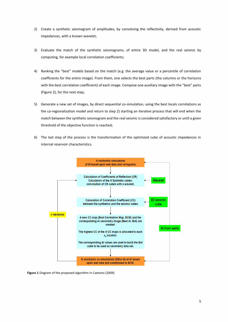
1) Generate a set of initial 3D models of acoustic impedances by using direct sequential simulation, instead
of individual traces or cells;
5
2) Create a synthetic seismogram of amplitudes, by convolving the reflectivity, derived from acoustic
impedances, with a known wavelet;
3) Evaluate the match of the synthetic seismograms, of entire 3D model, and the real seismic by
computing, for example local correlation coefficients;
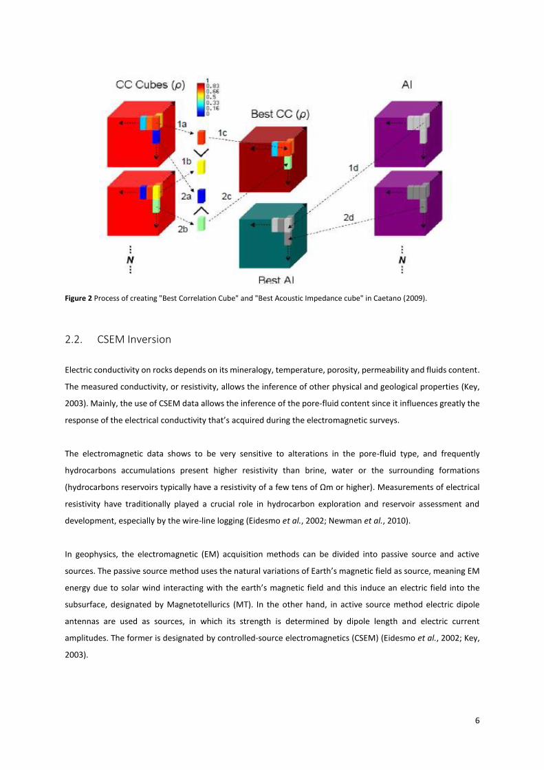
4) Ranking the “best” models based on the match (e.g. the average value or a percentile of correlation
coefficients for the entire image). From them, one selects the best parts (the columns or the horizons
with the best correlation coefficient) of each image. Compose one auxiliary image with the “best” parts
(Figure 2), for the next step;
5) Generate a new set of images, by direct sequential co-simulation, using the best locals correlations as
the co-regionalization model and return to step 2) starting an iterative process that will end when the
match between the synthetic seismogram and the real seismic is considered satisfactory or until a given
threshold of the objective function is reached;
6) The last step of the process is the transformation of the optimized cube of acoustic impedances in
internal reservoir characteristics.
Figure 1 Diagram of the proposed algorithm in Caetano (2009)
6
Figure 2 Process of creating "Best Correlation Cube" and "Best Acoustic Impedance cube" in Caetano (2009).
2.2. CSEM Inversion
Electric conductivity on rocks depends on its mineralogy, temperature, porosity, permeability and fluids content.
The measured conductivity, or resistivity, allows the inference of other physical and geological properties (Key,
2003). Mainly, the use of CSEM data allows the inference of the pore-fluid content since it influences greatly the
response of the electrical conductivity that’s acquired during the electromagnetic surveys.
The electromagnetic data shows to be very sensitive to alterations in the pore-fluid type, and frequently
hydrocarbons accumulations present higher resistivity than brine, water or the surrounding formations
(hydrocarbons reservoirs typically have a resistivity of a few tens of Ωm or higher). Measurements of electrical
resistivity have traditionally played a crucial role in hydrocarbon exploration and reservoir assessment and
development, especially by the wire-line logging (Eidesmo et al., 2002; Newman et al., 2010).
In geophysics, the electromagnetic (EM) acquisition methods can be divided into passive source and active
sources. The passive source method uses the natural variations of Earth’s magnetic field as source, meaning EM
energy due to solar wind interacting with the earth’s magnetic field and this induce an electric field into the
subsurface, designated by Magnetotellurics (MT). In the other hand, in active source method electric dipole
antennas are used as sources, in which its strength is determined by dipole length and electric current
amplitudes. The former is designated by controlled-source electromagnetics (CSEM) (Eidesmo et al., 2002; Key,
2003).

7
According to Eidesmo et al. (2002) both MT and CSEM responses can be obtained if the recording of EM data is
continued for a sufficiently long time. During CSEM analysis, the MT data is considered noise. The distinction
between them is possible, since CSEM data contain a set of frequency components depending on the source
signal and a set of different source-receiver offsets, whereas the marine MT data typically have a broader and
lower frequency spectrum.
The objective of an EM acquisition is to study the resistivity of the subsurface below the seafloor, through the
recording of magnetic and electric fields. Regarding the CSEM method the recorded fields are better in deep
water, and has become firmly established as an important geophysical tool in the offshore environment when
combined with seismic reflection data.
In terms of the acquisition, the more common geometries, use a mobile horizontal electric dipole (HED) source
and an array of seafloor electric receivers. The dipole emits a low frequency electromagnetic signal that diffuses
outwards. The rate of decay in amplitude and the phase shift of the signal are controlled both by geometric and
by skin depth effects (Eidesmo et al., 2002).
An example how the CSEM marine method works is presents in Constable and Srnka (2007) and summarized in
Figure 3:
1) On the deep seafloor, the seabed is normally more resistive than seawater, consequently the first data
recorded contain information about the geology. In the frequency domain, when the source-receiver
distance is adequate, the longer skin depths can be associated with seafloor rocks, once the field is
dominated by energy propagating through the geologic formations, and the energy propagating through
the seawater has absorbed and is absent from the signals. Furthermore, by concentrating all the
transmitter power into one frequency, large signal-to-noise rations can be achieved at larger source-
receiver offsets.
2) Electric fields are well suited to operation in seawater. Transmitter currents can be passed through
seawater reasonable power consumption and simple electrode systems. Receiver noise is very low
because cultural and MT noise is highly attenuated in the CSEM frequency-band. Magnetic field
receivers are employed, but motion sensors as water currents move the receiver instrument limits the
noise floor.

8
3) A horizontal electric dipole excites vertical and horizontal current flow in the seabed, maximizing
resolution for a variety of structures. A vertical magnetic dipole, for example, would excite mainly
horizontal current flow. Horizontal magnetic dipole also excite both vertical and horizontal currents, but
are less favored than electric dipoles for operational reasons.
Figure 3 Marine EM concepts: Electric and magnetic field receivers are deployed on the seafloor to record time-series measurements of the fields, which could be used to compute MT impedances. The seafloor instruments also receive signals emitted by a CSEM transmitter (towed close to the seafloor) at ranges of as much as about 10 km. The MT signals are associated with largely horizontal current flow in the seafloor, and are sensitive only to large-scale structures. The CSEM signals involve both vertical and horizontal current flow, which could be interrupted by oil and gas reservoirs to provide sensitivity to these geologic structures even when they are quite thin in Constable (2010).
Consequently, EM data give helpful information about the subsurface, in particular for the pore-fluid. For these
reasons there has been a great interest in developing new acquisition modes, inversion methodologies and, more
recently, the integration of this kind of data with seismic data.
According to Bosch et al. (2010) the process of inverting different types of geophysical data into the properties
of the subsurface, such as electrical or elastic properties, can be posed as an inverse problem. Hereupon, in this
case, the inverse problem poses as the resistivity model which is compatible with the EM data (Ray and Key,
2012).
The EM inversion problem is non-linear, ill-posed inverse problem, and according to Ray and Key (2012), the
approaches to solve the inverse problem depend on regularization methods that stabilizes the problem. The
results were smooth models or suite of smooth models as a function of data misfit.
Other methodologies to invert EM data are presented in Constable (2010), such as 1D frequency-domain solution
presented by Chave and Cox (1982); Flosadóttir and Constable (1996) altered the previous mentioned forward
code and implemented the regularized Occam’s inversion scheme of (Constable et al., 1987). Since then, several

9
other codes have been written, such as the fully anisotropic model of (Loseth and Ursin, 2007) and the code of
(Key, 2009).
Despite the advantages of using CSEM data there are practical limitations on the suitability of the technique
related with the intrinsic principles of the methodology, such as the impact of the airwave in shallower waters,
the limitations on depth of penetration and detectability imposed by absorption, and the thermal noise of the
transmitter-receiver system, frequency content restrictions from skin depths, that are not will be addressed in
this thesis, for more information please consult Constable (2010).
The CSEM technique by itself presents limitations, being more useful combined with other techniques, using a
multiproxy approach. That been said, a useful technique to combine with CSEM is seismic reflection data to
exclude lithological causes of high-resistivity near anomalous zones, such as sequences of evaporites, volcanics,
or carbonates (Gunning et al., 2010).
2.3. Joint Inversion
As it was possible to corroborate, the seismic inversion is an important tool for modeling and characterizing the
subsurface petro-elastic properties, while electromagnetic data is sensitive to the presence of fluids filling the
pore space.
The idea of jointly inverting this two types of data is quite recent and still is being developed. The main existing
methodologies were developed by Abubakar et al. (2012), Hoversten et al. (2006), Colombo et al (2008).
According to Abubakar et al. (2012) is possible to joint invert CSEM and seismic reflection data using two different
approaches:
The first one consists in invert petrophysical parameters (porosity, fluid saturations) by linking the
resistivity, seismic velocities, and the mass density to porosity and fluid saturations through
petrophysical relationships;
The second approach consists in enforce the structural similarity between resistivity and seismic velocity
of the targeted region using the cross-gradient approach.
Nevertheless, the joint inversion of these two types of data is not straightforward, considering that an inversion
reconstructs seismic velocities and mass-density distributions while electromagnetic inversion produces the
resistivity distribution.

10
Hoversten et al. (2006) proposed a joint seismic amplitude versus angle (AVA) and CSEM data inversion
employing 1D model parametrization. The inversion algorithm consists in a nonlinear least-squares problem, in
which we minimize the Tikhonov functional.
Gao et al (2012), on the other hand, presented a joint petrophysical inversion algorithm for CSEM and seismic
FWI, employing an acoustic approximation, for 2D configurations. The results presented show that the porosity
and water saturation maps were improved if one has a good a priori knowledge of the petrophysical relationship.
As can be verified, the joint inversion methodology of seismic data with EM data allows the access to models
that characterize better the reservoir parameters (electrical and elastic). Nevertheless, their difference in terms
of geophysical nature, needs the utilization of a rock physics model in order to link the elastic properties to the
petrophysical properties derived from the inverted resistivity models (Azevedo and Soares, 2014).
The rock physics models allow the characterization of the elastic moduli relying on factors, such as mineralogy,
porosity, pore type, pore fluids, clay content, sorting, cementation and stress (Bosch et al., 2010).
As stated, the connection between elastic and petrophysical properties is done by a rock physics model, that
allow to couple of both geophysical inverse problem within the same framework, the reservoir grid.
The calibration of the model is done by recurring to the well-log data available, meaning the data is used to
predict elastic attributes from petrophysical properties, and consists in a set of equations that transforms
petrophysical variables in elastic attributes (Grana and Rosa, 2010). For more information, please consult Avseth
et al. (2005).
11
3. Geostatistical Joint Inversion of seismic and EM
The proposed methodology for the joint inversion of seismic reflection and EM data, applied under the scope of
this thesis is an iterative geostatistical methodology where the model perturbation is performed by direct
sequential simulation (DSS) and co-simulation (co-DSS) (Soares, 2001). The convergence of the methodology
from iteration to iteration is ensured by a genetic algorithm, based on the cross-over principle, works as a global
optimizer to simultaneously converge the synthetic data into the real data. The inversion is finished when the
average global correlation coefficient between the real and inverted synthetic data, for both seismic and EM, is
above a threshold (Azevedo and Soares, 2014).
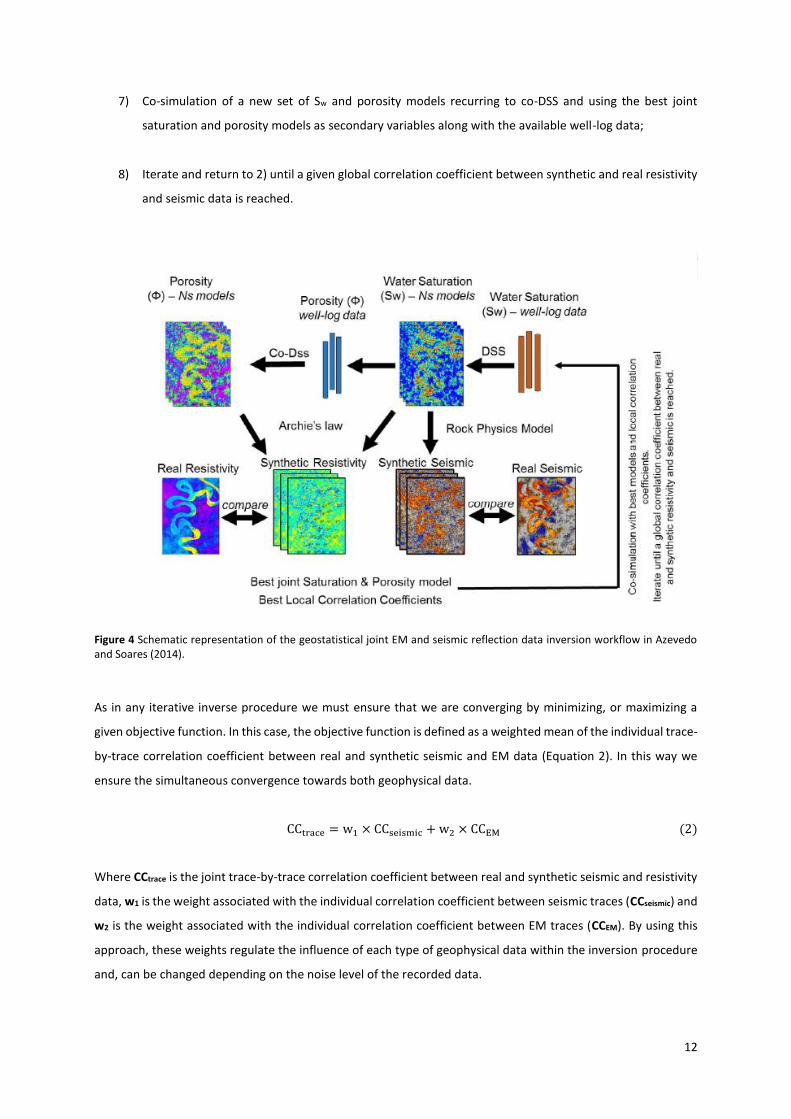
The geostatistical joint inversion of seismic and EM data can be summarized in the following sequence of steps
(Figure 4; Azevedo and Soares, 2014):
1) Simulation of Ns models of water saturation (Sw) recurring to stochastic sequential simulation DSS
(Soares, 2001) and using the available Sw-log data as experimental data for the simulation procedure;
2) Co-simulation of Ns porosity models using DSS with joint probability distributions (Horta and Soares,
2010), the available porosity well-log data as experimental data and each Sw model simulated in the
previous step as secondary variable;
3) Following Archie’s Law (Archie, 1942), calculate Ns synthetic resistivity responses for each pair of Sw and
porosity models simulated and co-simulated in the previous steps;
4) Following a pre-calibrated rock physics model at the wells locations, and for each porosity model
generated in 2), derive Ns acoustic impedance (AI) models and compute the corresponding normal
incidence synthetic seismic response;
5) Compute, in a trace-by-trace basis, the correlation coefficient between synthetic and real resistivity and
seismic responses;
6) Selection of the petro-elastic traces that simultaneously ensure the maximum correlation coefficient
between the recorded and the synthetic seismic data computed in the previous step. The individual
correlation coefficients are weighted averaged depending on the quality of the input geophysical data.
Save these elastic traces as the best joint saturation and porosity volumes among with the
corresponding correlation coefficients;
12
7) Co-simulation of a new set of Sw and porosity models recurring to co-DSS and using the best joint
saturation and porosity models as secondary variables along with the available well-log data;
8) Iterate and return to 2) until a given global correlation coefficient between synthetic and real resistivity
and seismic data is reached.
Figure 4 Schematic representation of the geostatistical joint EM and seismic reflection data inversion workflow in Azevedo and Soares (2014).
As in any iterative inverse procedure we must ensure that we are converging by minimizing, or maximizing a
given objective function. In this case, the objective function is defined as a weighted mean of the individual trace-
by-trace correlation coefficient between real and synthetic seismic and EM data (Equation 2). In this way we
ensure the simultaneous convergence towards both geophysical data.
CCtrace = w1 × CCseismic + w2 × CCEM (2)
Where CCtrace is the joint trace-by-trace correlation coefficient between real and synthetic seismic and resistivity
data, w1 is the weight associated with the individual correlation coefficient between seismic traces (CCseismic) and
w2 is the weight associated with the individual correlation coefficient between EM traces (CCEM). By using this
approach, these weights regulate the influence of each type of geophysical data within the inversion procedure
and, can be changed depending on the noise level of the recorded data.
13
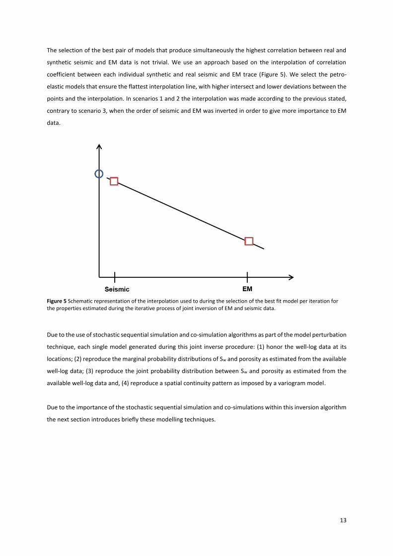
The selection of the best pair of models that produce simultaneously the highest correlation between real and
synthetic seismic and EM data is not trivial. We use an approach based on the interpolation of correlation
coefficient between each individual synthetic and real seismic and EM trace (Figure 5). We select the petro-
elastic models that ensure the flattest interpolation line, with higher intersect and lower deviations between the
points and the interpolation. In scenarios 1 and 2 the interpolation was made according to the previous stated,
contrary to scenario 3, when the order of seismic and EM was inverted in order to give more importance to EM
data.
Figure 5 Schematic representation of the interpolation used to during the selection of the best fit model per iteration for the properties estimated during the iterative process of joint inversion of EM and seismic data.
Due to the use of stochastic sequential simulation and co-simulation algorithms as part of the model perturbation
technique, each single model generated during this joint inverse procedure: (1) honor the well-log data at its
locations; (2) reproduce the marginal probability distributions of Sw and porosity as estimated from the available
well-log data; (3) reproduce the joint probability distribution between Sw and porosity as estimated from the
available well-log data and, (4) reproduce a spatial continuity pattern as imposed by a variogram model.
Due to the importance of the stochastic sequential simulation and co-simulations within this inversion algorithm
the next section introduces briefly these modelling techniques.

14
3.1. Direct sequential simulation and co-simulation with joint probability
distributions
The great advantage of using of the direct sequential simulation and co-simulation (Soares, 2001), when
compared with the traditional sequential Gaussian simulation, is due to the fact that is not required any Gaussian
transform of the experimental data. One can use the prior probability distribution estimated directly the
experimental data, i.e. the available well-log data.
The direct sequential simulation and co-simulation algorithm may be summarized in the following sequence of
steps (Soares, 2001):
1) Generate a random seed to define a random path over the entire simulation grid xi, i=1, …, N, where N
is the total number of nodes that compose the simulation grid;
2) Estimate the local mean and variance of Z(x0), being x0 the current simulation node, with simple kriging
estimate conditioned to the original experimental data (e.g. well-log data) and previously simulated
data of Z*(xi);
3) Draw a simulated value, Z*(x0), from the global conditional distribution function (cdf) of density, F(Z),
centered in the estimated local mean and with an interval defined by the estimated local variance;
4) Loop until all the N nodes of the grid have been simulated.
Since the traditional direct sequential co-simulation does guarantee the relationship between both primary and
secondary variables, as interpreted from the available experimental data, the use of direct sequential co-
simulation with joint distributions (Horta and Soares, 2010) was selected as the co-simulation methodology
within the proposed geostatistical joint inversion.
The sequential co-simulation procedure proposed in Horta and Soares (2010) ensures that:
The simulated model honors the bi-distribution between the model itself and the secondary variable;
The reproduction of the marginal probability distribution function of Z1 and Z2;
Their marginal covariance matrixes. The secondary variable must exist for all the nodes that compose
the simulation grid in order to be used as conditioning data un the estimation of the local mean and
variance by collocated co-kriging.

15
This stochastic sequential co-simulation with joint probability distributions can be summarized as follows (Horta
and Soares, 2010):
1) Estimate the global bi-distribution between the primary (Z1) and the secondary (Z2) variables;
2) Generate a random seed to define a random path over the entire simulation grid xi, i=1, …, N, where N
is the total number of nodes that compose the simulation grid;
3) Estimate the local mean and variance (collocated co-kriging) of Z1(x0), being x0 the current simulation
node, conditioned to the original experimental data (e.g. well-log data), previously simulated data of
Z1*(xi) and the collocated datum from the secondary variable - Z2
*(x0);
4) The conditional cumulative distribution (cdf) F[Z1(x0)|Z2(x0)] at the location x0 given the co-located value
of Z2(x0), is derived from the global joint probability distribution F(Z1, Z2);
5) The value Z1(x0) to be simulated is drawn from the cdf F[Z1(x0)|Z2(x0)] using a Monte Carlo sampling
technique;
6) Loop until all the N nodes of the simulation grid have been simulated.
3.2. Siliciclastic synthetic reservoir – Stanford VI-E
3.2.1. Dataset description
The structure of the Stanford VI reservoir is an asymmetric anticline, with axis N15ºE. Is represented as a three-
dimensional regular stratigraphic model with 150x200x200 cells. The dimension of the cells are 25m in the
horizontal direction (x and y), and 1m in the vertical direction (z). Therefore, the real reservoir size is 3750m by
5000m, with a thickness of 200m.
Stratigraphically, the Stanford VI reservoir corresponds to a fluvial channel system prograding into the basin
located toward the north of the reservoir (Lee and Mukerji, 2013). Deltaic deposits (layer 3) were formed first,
followed by the deposition of meandering channels (layer 2) and then sinuous channels (layer 1) in this fluvial
channel system.
The synthetic reservoir Stanford VI-E has three layers with different types of sedimentary deposition. In this
thesis, were only used the two first layers (Figure 6), with an inversion grid size of 150x200x120 cells. The layers
used for the joint inversion have 80m and 40m of thickness, respectively. They represent four facies: floodplain
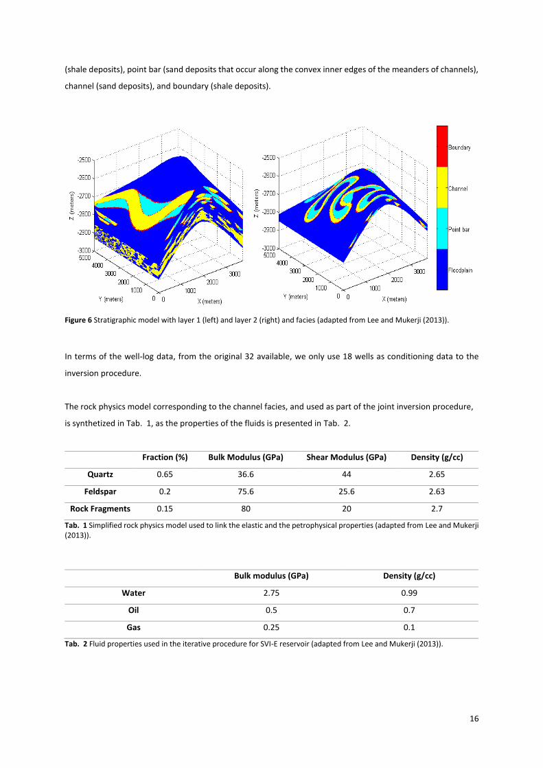
16
(shale deposits), point bar (sand deposits that occur along the convex inner edges of the meanders of channels),
channel (sand deposits), and boundary (shale deposits).
Figure 6 Stratigraphic model with layer 1 (left) and layer 2 (right) and facies (adapted from Lee and Mukerji (2013)).
In terms of the well-log data, from the original 32 available, we only use 18 wells as conditioning data to the
inversion procedure.
The rock physics model corresponding to the channel facies, and used as part of the joint inversion procedure,
is synthetized in Tab. 1, as the properties of the fluids is presented in Tab. 2.
Fraction (%) Bulk Modulus (GPa) Shear Modulus (GPa) Density (g/cc)
Quartz 0.65 36.6 44 2.65
Feldspar 0.2 75.6 25.6 2.63
Rock Fragments 0.15 80 20 2.7
Tab. 1 Simplified rock physics model used to link the elastic and the petrophysical properties (adapted from Lee and Mukerji (2013)).
Bulk modulus (GPa) Density (g/cc)
Water 2.75 0.99
Oil 0.5 0.7
Gas 0.25 0.1
Tab. 2 Fluid properties used in the iterative procedure for SVI-E reservoir (adapted from Lee and Mukerji (2013)).
17
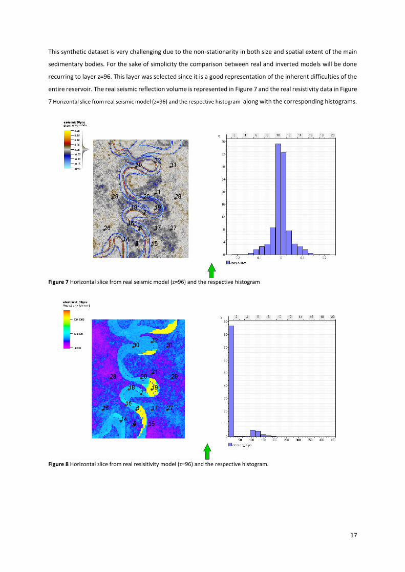
This synthetic dataset is very challenging due to the non-stationarity in both size and spatial extent of the main
sedimentary bodies. For the sake of simplicity the comparison between real and inverted models will be done
recurring to layer z=96. This layer was selected since it is a good representation of the inherent difficulties of the
entire reservoir. The real seismic reflection volume is represented in Figure 7 and the real resistivity data in Figure
7 Horizontal slice from real seismic model (z=96) and the respective histogram along with the corresponding histograms.
Figure 7 Horizontal slice from real seismic model (z=96) and the respective histogram
Figure 8 Horizontal slice from real resisitivity model (z=96) and the respective histogram.
18
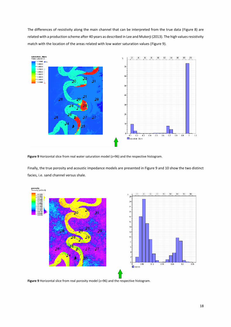
The differences of resistivity along the main channel that can be interpreted from the true data (Figure 8) are
related with a production scheme after 40 years as described in Lee and Mukerji (2013). The high values resistivity
match with the location of the areas related with low water saturation values (Figure 9).
Figure 9 Horizontal slice from real water saturation model (z=96) and the respective histogram.
Finally, the true porosity and acoustic impedance models are presented in Figure 9 and 10 show the two distinct
facies, i.e. sand channel versus shale.
Figure 9 Horizontal slice from real porosity model (z=96) and the respective histogram.
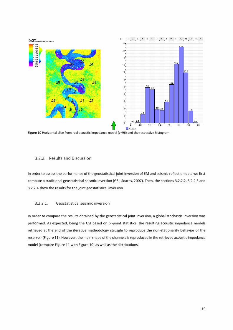
19
Figure 10 Horizontal slice from real acoustic impedance model (z=96) and the respective histogram.
3.2.2. Results and Discussion
In order to assess the performance of the geostatistical joint inversion of EM and seismic reflection data we first
compute a traditional geostatistical seismic inversion (GSI; Soares, 2007). Then, the sections 3.2.2.2, 3.2.2.3 and
3.2.2.4 show the results for the joint geostatistical inversion.
3.2.2.1. Geostatistical seismic inversion
In order to compare the results obtained by the geostatistical joint inversion, a global stochastic inversion was
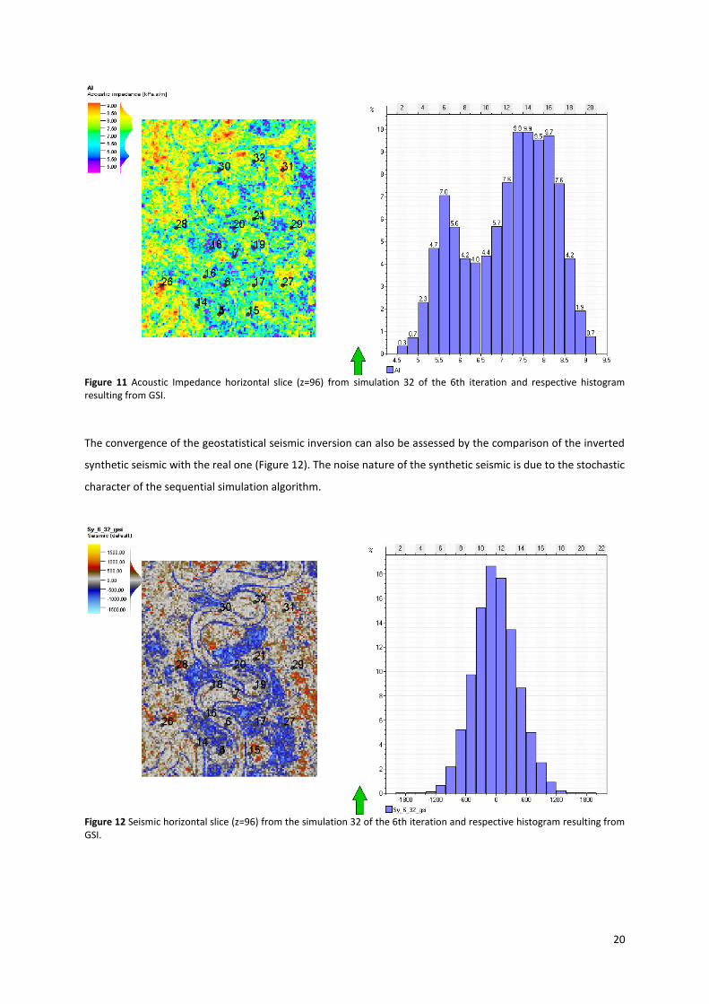
performed. As expected, being the GSI based on bi-point statistics, the resulting acoustic impedance models
retrieved at the end of the iterative methodology struggle to reproduce the non-stationarity behavior of the
reservoir (Figure 11). However, the main shape of the channels is reproduced in the retrieved acoustic impedance
model (compare Figure 11 with Figure 10) as well as the distributions.
20
Figure 11 Acoustic Impedance horizontal slice (z=96) from simulation 32 of the 6th iteration and respective histogram resulting from GSI.
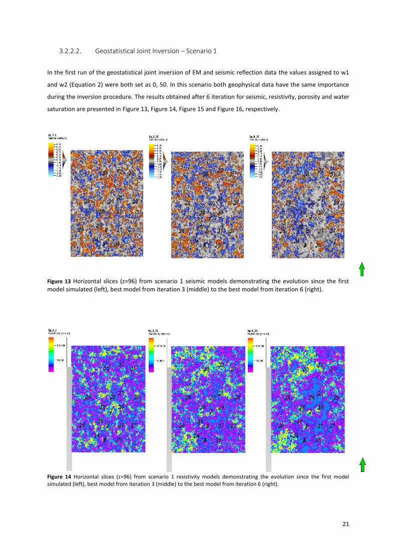
The convergence of the geostatistical seismic inversion can also be assessed by the comparison of the inverted
synthetic seismic with the real one (Figure 12). The noise nature of the synthetic seismic is due to the stochastic
character of the sequential simulation algorithm.
Figure 12 Seismic horizontal slice (z=96) from the simulation 32 of the 6th iteration and respective histogram resulting from GSI.
21
3.2.2.2. Geostatistical Joint Inversion – Scenario 1
In the first run of the geostatistical joint inversion of EM and seismic reflection data the values assigned to w1
and w2 (Equation 2) were both set as 0, 50. In this scenario both geophysical data have the same importance
during the inversion procedure. The results obtained after 6 iteration for seismic, resistivity, porosity and water
saturation are presented in Figure 13, Figure 14, Figure 15 and Figure 16, respectively.
Figure 13 Horizontal slices (z=96) from scenario 1 seismic models demonstrating the evolution since the first model simulated (left), best model from iteration 3 (middle) to the best model from iteration 6 (right).
Figure 14 Horizontal slices (z=96) from scenario 1 resistivity models demonstrating the evolution since the first model simulated (left), best model from iteration 3 (middle) to the best model from iteration 6 (right).
22
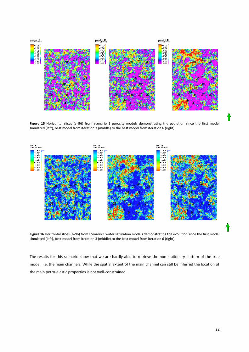
Figure 15 Horizontal slices (z=96) from scenario 1 porosity models demonstrating the evolution since the first model simulated (left), best model from iteration 3 (middle) to the best model from iteration 6 (right).
Figure 16 Horizontal slices (z=96) from scenario 1 water saturation models demonstrating the evolution since the first model simulated (left), best model from iteration 3 (middle) to the best model from iteration 6 (right).
The results for this scenario show that we are hardly able to retrieve the non-stationary pattern of the true
model, i.e. the main channels. While the spatial extent of the main channel can still be inferred the location of
the main petro-elastic properties is not well-constrained.
23
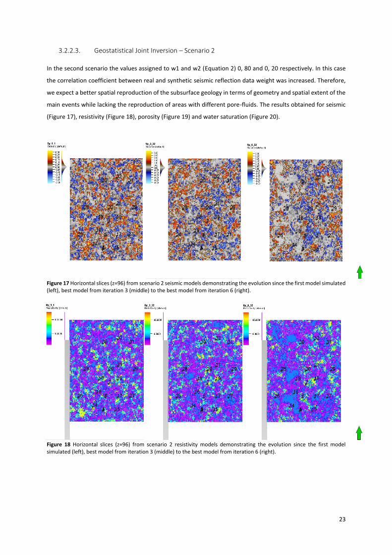
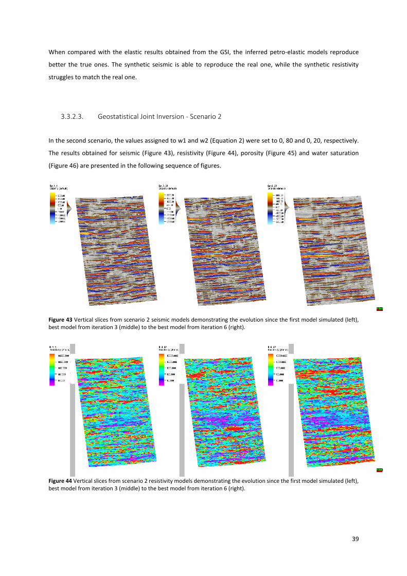
3.2.2.3. Geostatistical Joint Inversion – Scenario 2
In the second scenario the values assigned to w1 and w2 (Equation 2) 0, 80 and 0, 20 respectively. In this case
the correlation coefficient between real and synthetic seismic reflection data weight was increased. Therefore,
we expect a better spatial reproduction of the subsurface geology in terms of geometry and spatial extent of the
main events while lacking the reproduction of areas with different pore-fluids. The results obtained for seismic
(Figure 17), resistivity (Figure 18), porosity (Figure 19) and water saturation (Figure 20).
Figure 17 Horizontal slices (z=96) from scenario 2 seismic models demonstrating the evolution since the first model simulated (left), best model from iteration 3 (middle) to the best model from iteration 6 (right).
Figure 18 Horizontal slices (z=96) from scenario 2 resistivity models demonstrating the evolution since the first model simulated (left), best model from iteration 3 (middle) to the best model from iteration 6 (right).
24
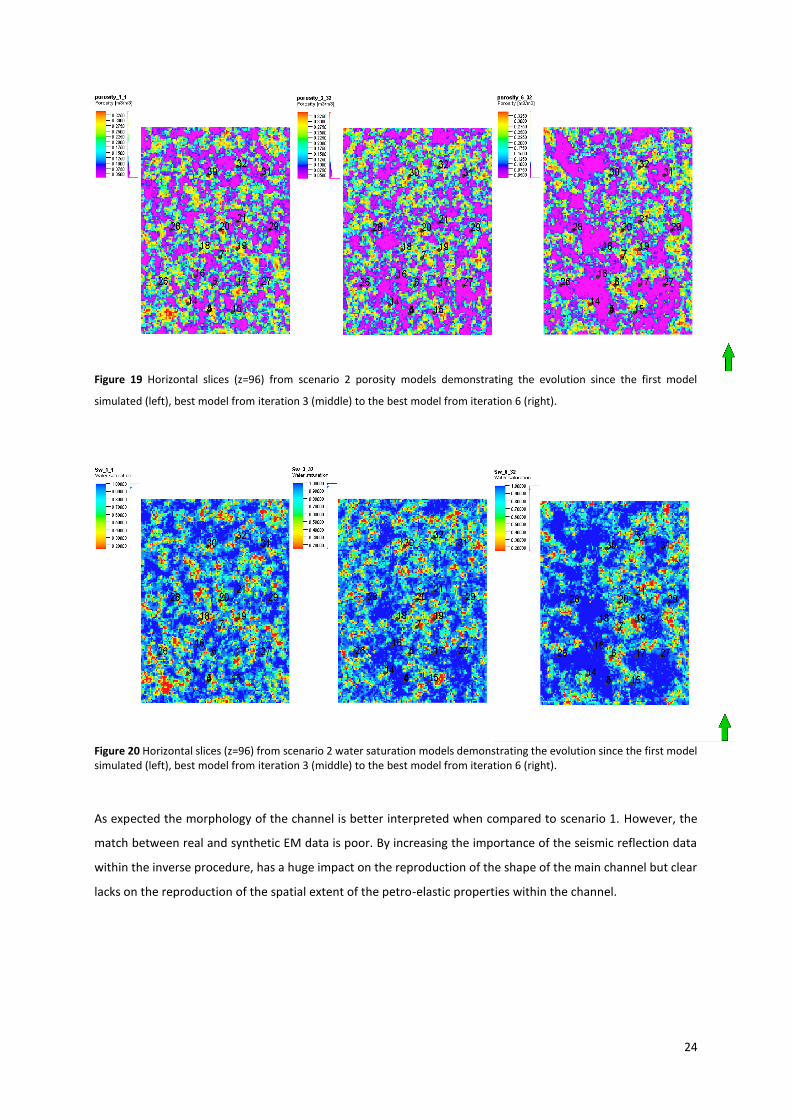
Figure 19 Horizontal slices (z=96) from scenario 2 porosity models demonstrating the evolution since the first model
simulated (left), best model from iteration 3 (middle) to the best model from iteration 6 (right).
Figure 20 Horizontal slices (z=96) from scenario 2 water saturation models demonstrating the evolution since the first model simulated (left), best model from iteration 3 (middle) to the best model from iteration 6 (right).
As expected the morphology of the channel is better interpreted when compared to scenario 1. However, the
match between real and synthetic EM data is poor. By increasing the importance of the seismic reflection data
within the inverse procedure, has a huge impact on the reproduction of the shape of the main channel but clear
lacks on the reproduction of the spatial extent of the petro-elastic properties within the channel.

25
3.2.2.4. Geostatistical Joint Inversion – Scenario 3
In the third scenario the values assigned to w1 and w2 were 0, 80 and 0, 20 respectively, but interpolation the
local correlation coefficients from EM do seismic data, i.e. the opposite order of the previous scenarios. The
results obtained for seismic (Figure 21), resistivity (Figure 22), porosity (Figure 23) and water saturation (Figure
24).
Figure 21 Horizontal slices (z=96) from scenario 3 seismic models demonstrating the evolution since the first model simulated
(left), best model from iteration 3 (middle) to the best model from iteration 6 (right).
Figure 22 Horizontal slices (z=96) from scenario 3 resistivity models demonstrating the evolution since the first model simulated (left), best model from iteration 3 (middle) to the best model from iteration 6 (right).
26
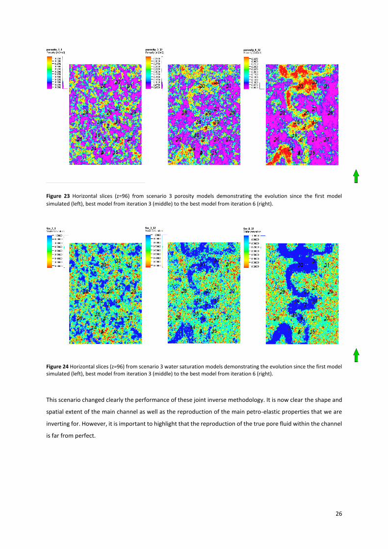
Figure 23 Horizontal slices (z=96) from scenario 3 porosity models demonstrating the evolution since the first model
simulated (left), best model from iteration 3 (middle) to the best model from iteration 6 (right).
Figure 24 Horizontal slices (z=96) from scenario 3 water saturation models demonstrating the evolution since the first model simulated (left), best model from iteration 3 (middle) to the best model from iteration 6 (right).
This scenario changed clearly the performance of these joint inverse methodology. It is now clear the shape and
spatial extent of the main channel as well as the reproduction of the main petro-elastic properties that we are
inverting for. However, it is important to highlight that the reproduction of the true pore fluid within the channel
is far from perfect.
27
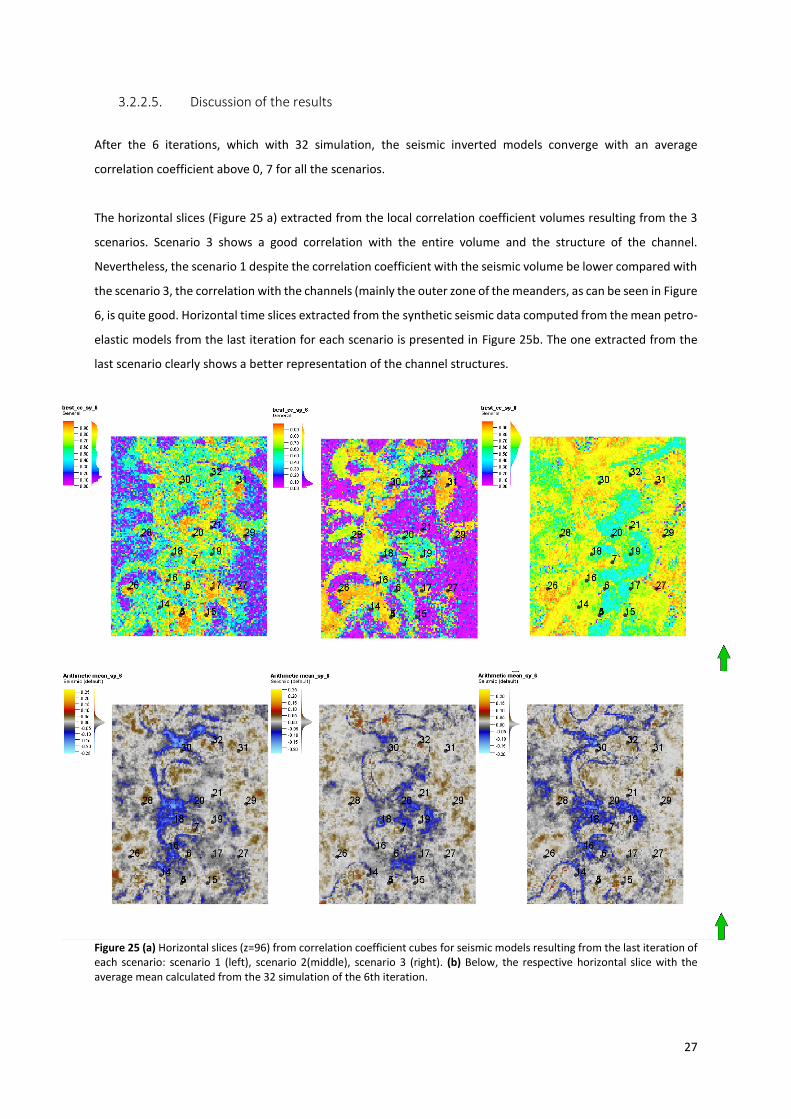
3.2.2.5. Discussion of the results
After the 6 iterations, which with 32 simulation, the seismic inverted models converge with an average
correlation coefficient above 0, 7 for all the scenarios.
The horizontal slices (Figure 25 a) extracted from the local correlation coefficient volumes resulting from the 3
scenarios. Scenario 3 shows a good correlation with the entire volume and the structure of the channel.
Nevertheless, the scenario 1 despite the correlation coefficient with the seismic volume be lower compared with
the scenario 3, the correlation with the channels (mainly the outer zone of the meanders, as can be seen in Figure
6, is quite good. Horizontal time slices extracted from the synthetic seismic data computed from the mean petro-
elastic models from the last iteration for each scenario is presented in Figure 25b. The one extracted from the
last scenario clearly shows a better representation of the channel structures.
Figure 25 (a) Horizontal slices (z=96) from correlation coefficient cubes for seismic models resulting from the last iteration of each scenario: scenario 1 (left), scenario 2(middle), scenario 3 (right). (b) Below, the respective horizontal slice with the average mean calculated from the 32 simulation of the 6th iteration.
28
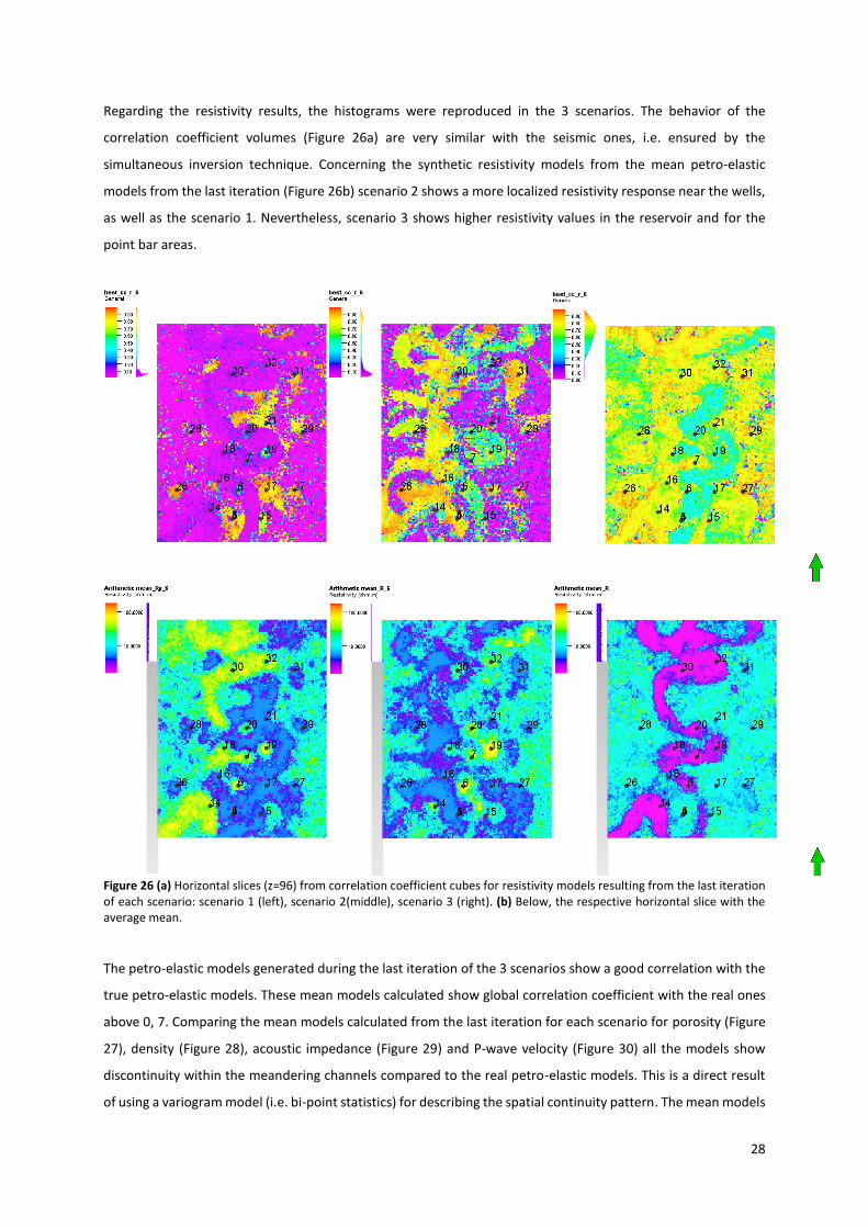
Regarding the resistivity results, the histograms were reproduced in the 3 scenarios. The behavior of the
correlation coefficient volumes (Figure 26a) are very similar with the seismic ones, i.e. ensured by the
simultaneous inversion technique. Concerning the synthetic resistivity models from the mean petro-elastic
models from the last iteration (Figure 26b) scenario 2 shows a more localized resistivity response near the wells,
as well as the scenario 1. Nevertheless, scenario 3 shows higher resistivity values in the reservoir and for the
point bar areas.
Figure 26 (a) Horizontal slices (z=96) from correlation coefficient cubes for resistivity models resulting from the last iteration of each scenario: scenario 1 (left), scenario 2(middle), scenario 3 (right). (b) Below, the respective horizontal slice with the average mean.
The petro-elastic models generated during the last iteration of the 3 scenarios show a good correlation with the
true petro-elastic models. These mean models calculated show global correlation coefficient with the real ones
above 0, 7. Comparing the mean models calculated from the last iteration for each scenario for porosity (Figure
27), density (Figure 28), acoustic impedance (Figure 29) and P-wave velocity (Figure 30) all the models show
discontinuity within the meandering channels compared to the real petro-elastic models. This is a direct result
of using a variogram model (i.e. bi-point statistics) for describing the spatial continuity pattern. The mean models
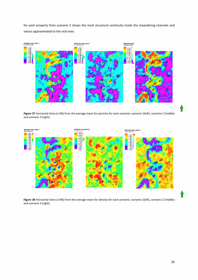
29
for each property from scenario 3 shows the most structural continuity inside the meandering channels and
values approximated to the real ones.
Figure 27 Horizontal slices (z=96) from the average mean for porosity for each scenario: scenario 1(left), scenario 2 (middle) and scenario 3 (right).
Figure 28 Horizontal slices (z=96) from the average mean for density for each scenario: scenario 1(left), scenario 2 (middle) and scenario 3 (right).
30
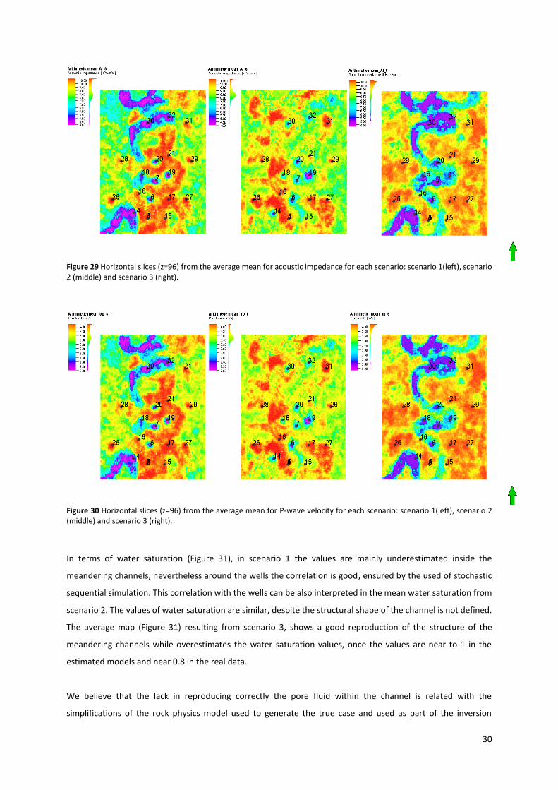
Figure 29 Horizontal slices (z=96) from the average mean for acoustic impedance for each scenario: scenario 1(left), scenario 2 (middle) and scenario 3 (right).
Figure 30 Horizontal slices (z=96) from the average mean for P-wave velocity for each scenario: scenario 1(left), scenario 2 (middle) and scenario 3 (right).
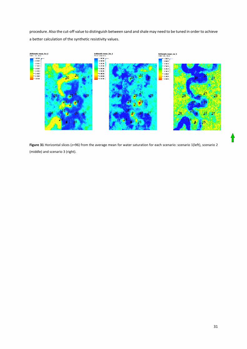
In terms of water saturation (Figure 31), in scenario 1 the values are mainly underestimated inside the
meandering channels, nevertheless around the wells the correlation is good, ensured by the used of stochastic
sequential simulation. This correlation with the wells can be also interpreted in the mean water saturation from
scenario 2. The values of water saturation are similar, despite the structural shape of the channel is not defined.
The average map (Figure 31) resulting from scenario 3, shows a good reproduction of the structure of the
meandering channels while overestimates the water saturation values, once the values are near to 1 in the
estimated models and near 0.8 in the real data.
We believe that the lack in reproducing correctly the pore fluid within the channel is related with the
simplifications of the rock physics model used to generate the true case and used as part of the inversion
31
procedure. Also the cut-off value to distinguish between sand and shale may need to be tuned in order to achieve
a better calculation of the synthetic resistivity values.
Figure 31 Horizontal slices (z=96) from the average mean for water saturation for each scenario: scenario 1(left), scenario 2
(middle) and scenario 3 (right).

32
3.3. Carbonate synthetic reservoir – CERENA-I
3.3.1. Dataset description
CERENA -I is a synthetic model created to recreate Brazilian Pre-salt carbonate fields. This model has a corner-
point grid with 161x161x300 cells, with 25x25x1 m spacing. The geological facies model tries to translate the
evolution of sedimentary environments on the early stages of a carbonate basin (Pinto, 2014).
This model presents two facies: the reservoir facies, composed by microbiolites and the non-reservoir facies
composed by mudstones. These are located in three distinct stratigraphic units of approximately 100m thickness.
The lower unit is strongly laminated (1 to 2m), microbiolites alternating with limestones with mudstone texture,
representing inter-tidal or lagoon environments. The middle unit contains dome-shaped geometries
representing reef formations. The top unit is composed of lenticular bodies (microbiolites), corresponding to a
marine environment. The facies were modelled recurring to object-based modeling.
From the initial carbonate model a fine grid sectorial model was extracted in order to speed-up the iterative
procedure. Despite being considerably smaller, this sectorial model reproduces the total variability of the full
field, instead of and up scaled model.
Hereupon, from the 16km2 and 7 million cell full field model, a 1 km2 and 280.000 active cells model was created.
The rock physics model used in the joint inversion procedure (Tab. 3 and Tab. 4) correspond to the floodplain
facies. Notice that this rock physics model describes the behavior of a carbonate field, i.e. the Xu-Payne mode
was used to model the petro-elastic properties of the model.
Fraction (%) Bulk modulus (GPa) Shear modulus (GPa) Density (g/cc)
Quartz 0.1 37 44 2.65
Aragonite 0.05 44.8 38.8 2.9
Calcite 0.85 76.8 32 2.7
Tab. 3 Simplified rock physics model used to link the elastic and the petrophysical properties ( adapted from Pinto (2014)).
Bulk modulus (Gpa) Density (g/cc)
Water 2.57 0.99
Oil 3.07 0.97
Gas 0.25 1.33
Tab. 4 Fluids properties used in the iterative process for CERENA-I
33
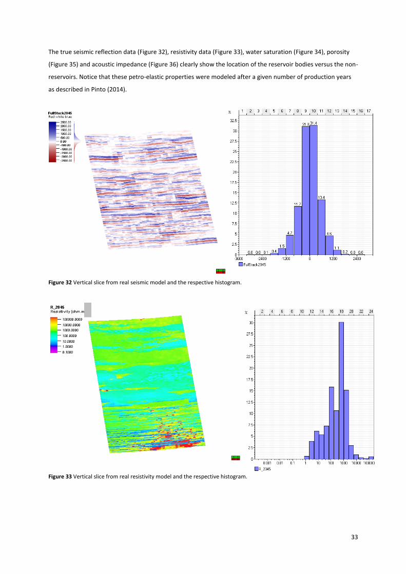
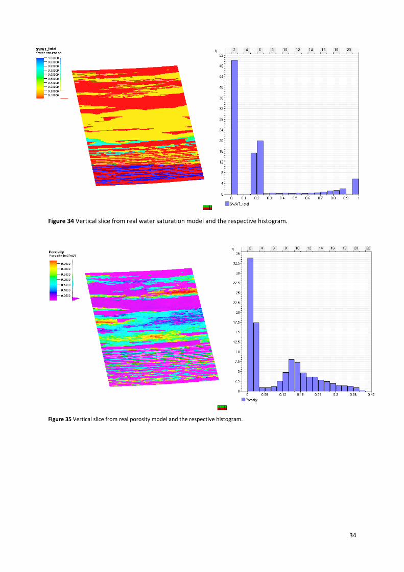
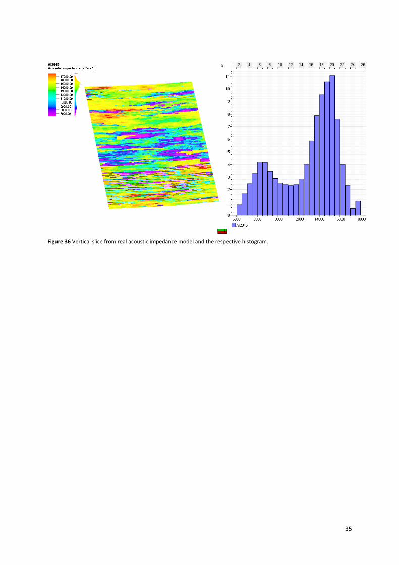
The true seismic reflection data (Figure 32), resistivity data (Figure 33), water saturation (Figure 34), porosity
(Figure 35) and acoustic impedance (Figure 36) clearly show the location of the reservoir bodies versus the non-
reservoirs. Notice that these petro-elastic properties were modeled after a given number of production years
as described in Pinto (2014).
Figure 32 Vertical slice from real seismic model and the respective histogram.
Figure 33 Vertical slice from real resistivity model and the respective histogram.
34
Figure 34 Vertical slice from real water saturation model and the respective histogram.
Figure 35 Vertical slice from real porosity model and the respective histogram.
35
Figure 36 Vertical slice from real acoustic impedance model and the respective histogram.
36
3.3.2. Results and Discussion
In this section we present first the results from the GSI (3.3.2.1), followed by the results for the joint inversion
based on different scenarios: scenario 1 (3.3.2.2) and scenario 2 (3.3.2.3), scenario 3 (3.3.2.4).
3.3.2.1. Geostatistical Seismic Inversion - GSI
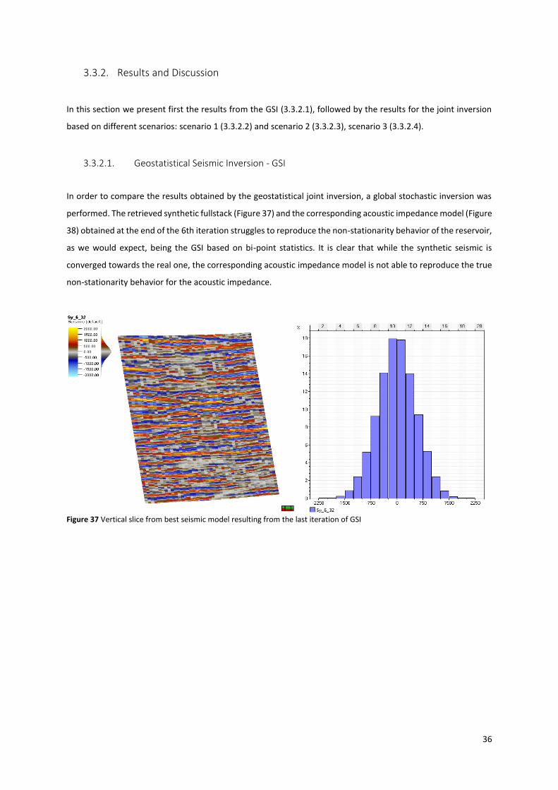
In order to compare the results obtained by the geostatistical joint inversion, a global stochastic inversion was
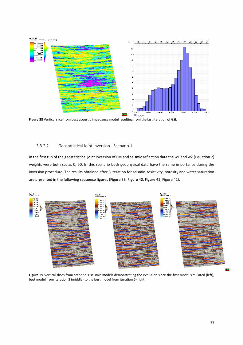
performed. The retrieved synthetic fullstack (Figure 37) and the corresponding acoustic impedance model (Figure
38) obtained at the end of the 6th iteration struggles to reproduce the non-stationarity behavior of the reservoir,
as we would expect, being the GSI based on bi-point statistics. It is clear that while the synthetic seismic is
converged towards the real one, the corresponding acoustic impedance model is not able to reproduce the true
non-stationarity behavior for the acoustic impedance.
Figure 37 Vertical slice from best seismic model resulting from the last iteration of GSI
37
Figure 38 Vertical slice from best acoustic impedance model resulting from the last iteration of GSI.
3.3.2.2. Geostatistical Joint Inversion - Scenario 1
In the first run of the geostatistical joint inversion of EM and seismic reflection data the w1 and w2 (Equation 2)
weights were both set as 0, 50. In this scenario both geophysical data have the same importance during the
inversion procedure. The results obtained after 6 iteration for seismic, resistivity, porosity and water saturation
are presented in the following sequence figures (Figure 39, Figure 40, Figure 41, Figure 42).
Figure 39 Vertical slices from scenario 1 seismic models demonstrating the evolution since the first model simulated (left), best model from iteration 3 (middle) to the best model from iteration 6 (right).
38
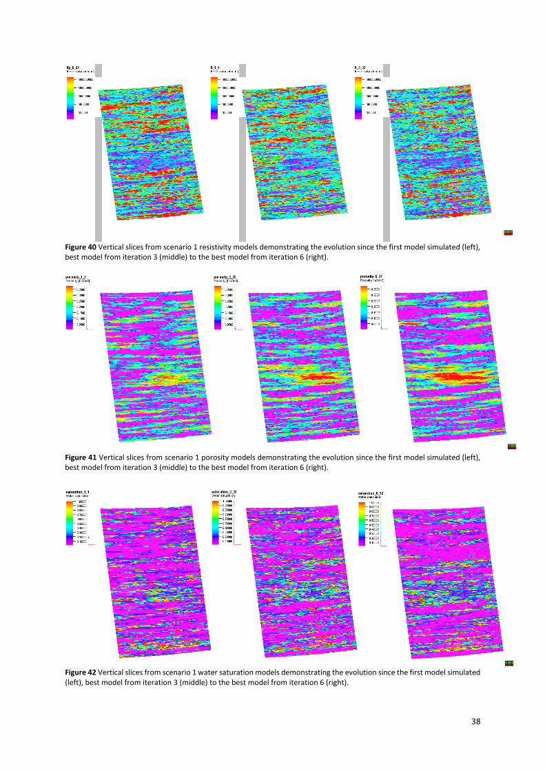
Figure 40 Vertical slices from scenario 1 resistivity models demonstrating the evolution since the first model simulated (left), best model from iteration 3 (middle) to the best model from iteration 6 (right).
Figure 41 Vertical slices from scenario 1 porosity models demonstrating the evolution since the first model simulated (left), best model from iteration 3 (middle) to the best model from iteration 6 (right).
Figure 42 Vertical slices from scenario 1 water saturation models demonstrating the evolution since the first model simulated (left), best model from iteration 3 (middle) to the best model from iteration 6 (right).
39
When compared with the elastic results obtained from the GSI, the inferred petro-elastic models reproduce
better the true ones. The synthetic seismic is able to reproduce the real one, while the synthetic resistivity
struggles to match the real one.
3.3.2.3. Geostatistical Joint Inversion - Scenario 2
In the second scenario, the values assigned to w1 and w2 (Equation 2) were set to 0, 80 and 0, 20, respectively.
The results obtained for seismic (Figure 43), resistivity (Figure 44), porosity (Figure 45) and water saturation
(Figure 46) are presented in the following sequence of figures.
Figure 43 Vertical slices from scenario 2 seismic models demonstrating the evolution since the first model simulated (left), best model from iteration 3 (middle) to the best model from iteration 6 (right).
Figure 44 Vertical slices from scenario 2 resistivity models demonstrating the evolution since the first model simulated (left), best model from iteration 3 (middle) to the best model from iteration 6 (right).
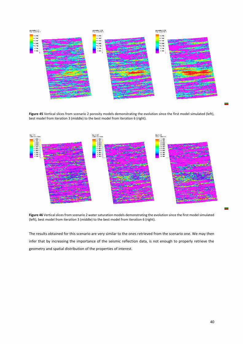
40
Figure 45 Vertical slices from scenario 2 porosity models demonstrating the evolution since the first model simulated (left), best model from iteration 3 (middle) to the best model from iteration 6 (right).
Figure 46 Vertical slices from scenario 2 water saturation models demonstrating the evolution since the first model simulated (left), best model from iteration 3 (middle) to the best model from iteration 6 (right).
The results obtained for this scenario are very similar to the ones retrieved from the scenario one. We may then
infer that by increasing the importance of the seismic reflection data, is not enough to properly retrieve the
geometry and spatial distribution of the properties of interest.
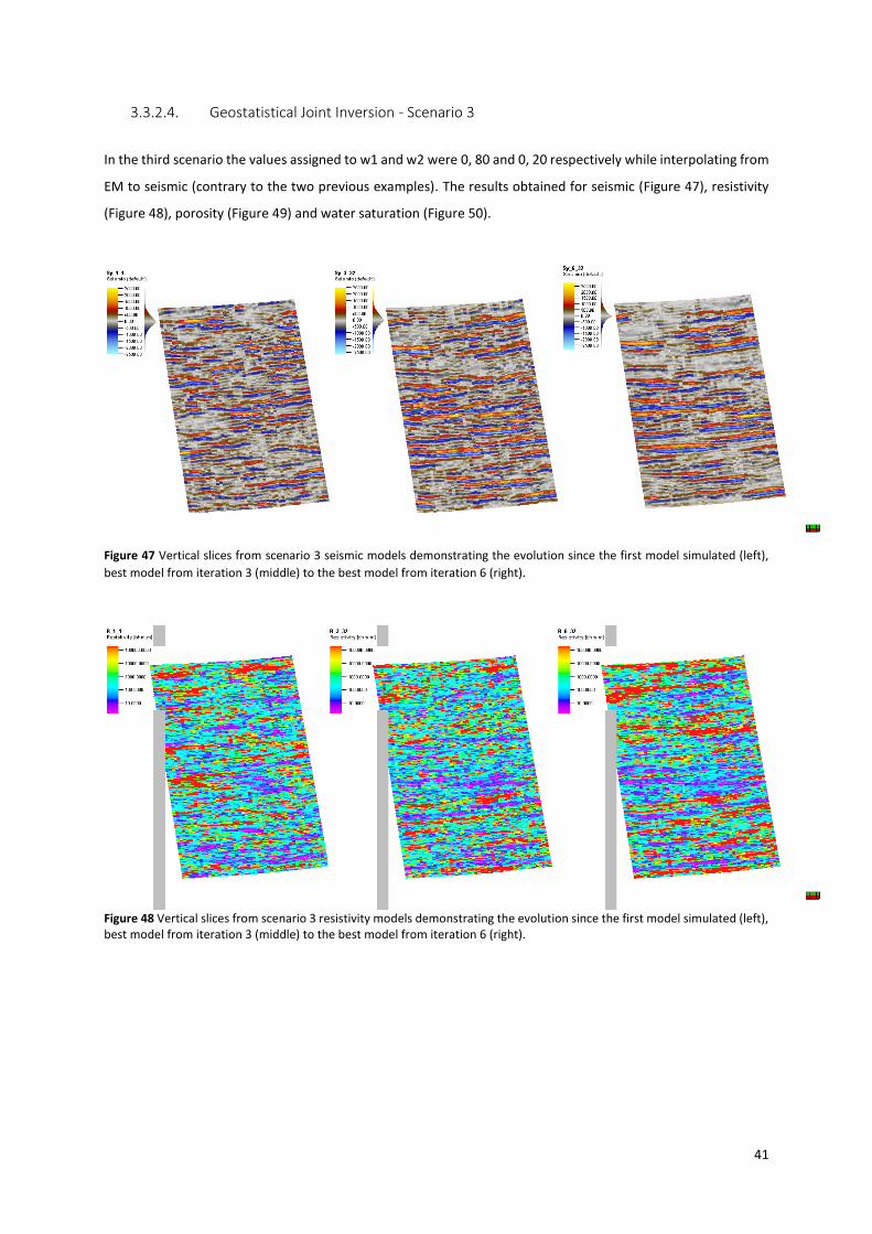
41
3.3.2.4. Geostatistical Joint Inversion - Scenario 3
In the third scenario the values assigned to w1 and w2 were 0, 80 and 0, 20 respectively while interpolating from
EM to seismic (contrary to the two previous examples). The results obtained for seismic (Figure 47), resistivity
(Figure 48), porosity (Figure 49) and water saturation (Figure 50).
Figure 47 Vertical slices from scenario 3 seismic models demonstrating the evolution since the first model simulated (left),
best model from iteration 3 (middle) to the best model from iteration 6 (right).
Figure 48 Vertical slices from scenario 3 resistivity models demonstrating the evolution since the first model simulated (left), best model from iteration 3 (middle) to the best model from iteration 6 (right).
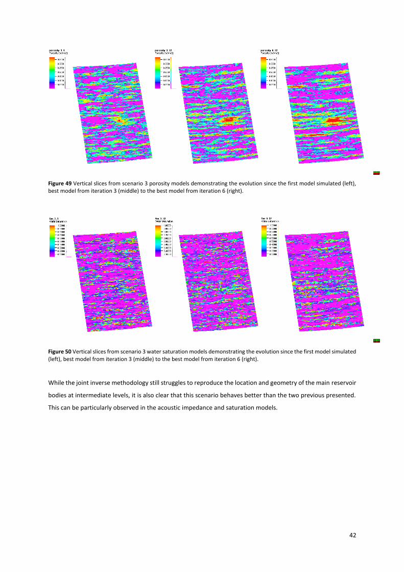
42
Figure 49 Vertical slices from scenario 3 porosity models demonstrating the evolution since the first model simulated (left), best model from iteration 3 (middle) to the best model from iteration 6 (right).
Figure 50 Vertical slices from scenario 3 water saturation models demonstrating the evolution since the first model simulated (left), best model from iteration 3 (middle) to the best model from iteration 6 (right).
While the joint inverse methodology still struggles to reproduce the location and geometry of the main reservoir
bodies at intermediate levels, it is also clear that this scenario behaves better than the two previous presented.
This can be particularly observed in the acoustic impedance and saturation models.
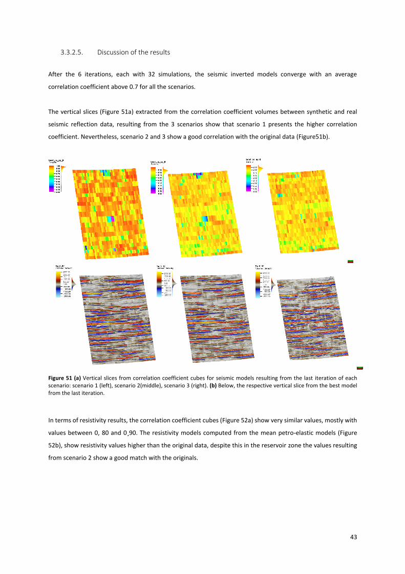
43
3.3.2.5. Discussion of the results
After the 6 iterations, each with 32 simulations, the seismic inverted models converge with an average
correlation coefficient above 0.7 for all the scenarios.
The vertical slices (Figure 51a) extracted from the correlation coefficient volumes between synthetic and real
seismic reflection data, resulting from the 3 scenarios show that scenario 1 presents the higher correlation
coefficient. Nevertheless, scenario 2 and 3 show a good correlation with the original data (Figure51b).
Figure 51 (a) Vertical slices from correlation coefficient cubes for seismic models resulting from the last iteration of each scenario: scenario 1 (left), scenario 2(middle), scenario 3 (right). (b) Below, the respective vertical slice from the best model from the last iteration.
In terms of resistivity results, the correlation coefficient cubes (Figure 52a) show very similar values, mostly with
values between 0, 80 and 0¸90. The resistivity models computed from the mean petro-elastic models (Figure
52b), show resistivity values higher than the original data, despite this in the reservoir zone the values resulting
from scenario 2 show a good match with the originals.
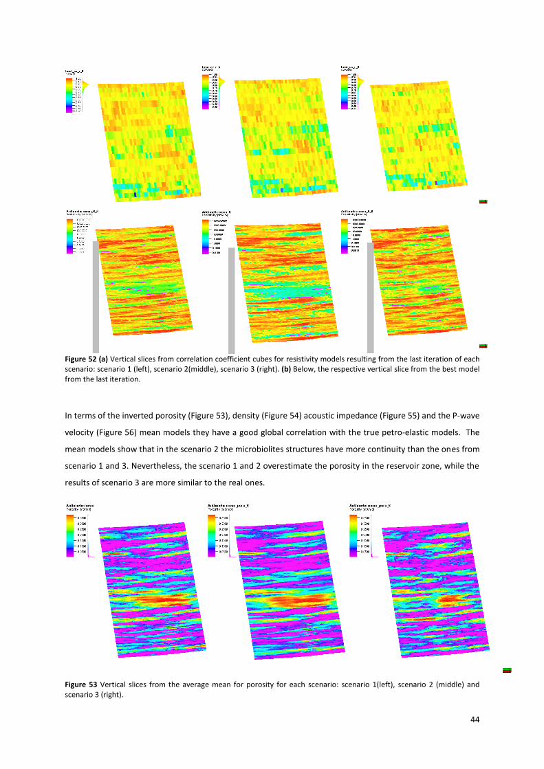
44
Figure 52 (a) Vertical slices from correlation coefficient cubes for resistivity models resulting from the last iteration of each scenario: scenario 1 (left), scenario 2(middle), scenario 3 (right). (b) Below, the respective vertical slice from the best model from the last iteration.
In terms of the inverted porosity (Figure 53), density (Figure 54) acoustic impedance (Figure 55) and the P-wave
velocity (Figure 56) mean models they have a good global correlation with the true petro-elastic models. The
mean models show that in the scenario 2 the microbiolites structures have more continuity than the ones from
scenario 1 and 3. Nevertheless, the scenario 1 and 2 overestimate the porosity in the reservoir zone, while the
results of scenario 3 are more similar to the real ones.
Figure 53 Vertical slices from the average mean for porosity for each scenario: scenario 1(left), scenario 2 (middle) and scenario 3 (right).
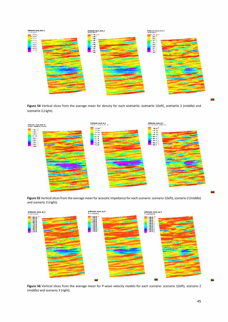
45
Figure 54 Vertical slices from the average mean for density for each scenario: scenario 1(left), scenario 2 (middle) and
scenario 3 (right).
Figure 55 Vertical slices from the average mean for acoustic impedance for each scenario: scenario 1(left), scenario 2 (middle) and scenario 3 (right).
Figure 56 Vertical slices from the average mean for P-wave velocity models for each scenario: scenario 1(left), scenario 2 (middle) and scenario 3 (right).
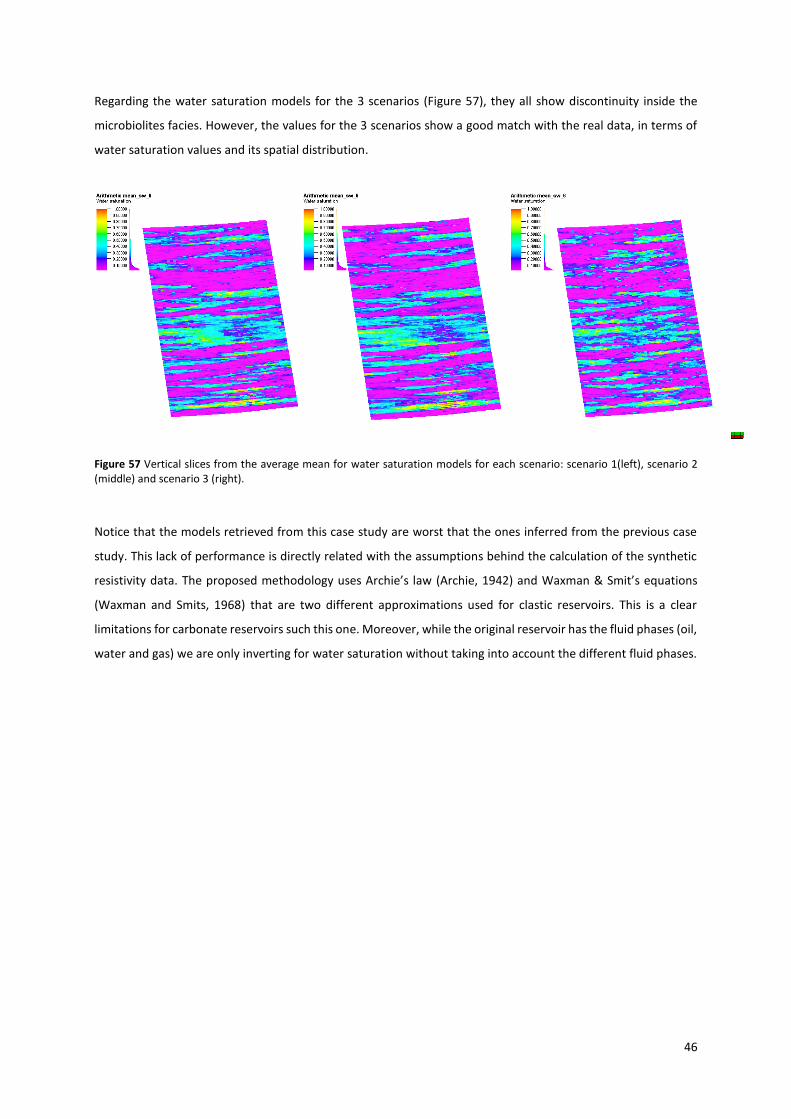
46
Regarding the water saturation models for the 3 scenarios (Figure 57), they all show discontinuity inside the
microbiolites facies. However, the values for the 3 scenarios show a good match with the real data, in terms of
water saturation values and its spatial distribution.
Figure 57 Vertical slices from the average mean for water saturation models for each scenario: scenario 1(left), scenario 2 (middle) and scenario 3 (right).
Notice that the models retrieved from this case study are worst that the ones inferred from the previous case
study. This lack of performance is directly related with the assumptions behind the calculation of the synthetic
resistivity data. The proposed methodology uses Archie’s law (Archie, 1942) and Waxman & Smit’s equations
(Waxman and Smits, 1968) that are two different approximations used for clastic reservoirs. This is a clear
limitations for carbonate reservoirs such this one. Moreover, while the original reservoir has the fluid phases (oil,
water and gas) we are only inverting for water saturation without taking into account the different fluid phases.

47
4. Conclusions and further recommendations
The main objective of this thesis was the implementation of a new iterative joint geostatistical seismic and EM
inversion methodology to two different case studies and comparing the resulting models with a conventional
seismic inversion methodology. There was an improvement of the inverted properties, with more accurate
acoustic impedance models for both reservoirs. In addition, we are able not only to derive acoustic impedance
but also petrophysical properties of interest such as water saturation and porosity.
In order hand, comparing the results from the different scenarios of the new iterative geostatistical inversion
methodology for joint inversion of EM and seismic data, for both reservoirs the main lithological structures were
reproduced, despite the spatial discontinuity inside the meandering channels (SVI-E) and the microbiolites
(CERENA-I).
The inverted models resultant from the joint inversion for petro-elastic properties showed a good matched with
the real data. For SVI-E the best inferred models were resulting from scenario 3 and for CERENA-I the models
from scenario 2, despite in the last synthetic reservoir the results are similar for the two scenarios. In terms of
water saturation models the algorithm struggles to converge to the solution. For both reservoirs, outside the
reservoir facies, the data shows a mismatch with the real ones. This mismatch may be explained by the use of
Archie’s law and Waxman and Smit’s equation in different lithologies than the clastic ones, for water saturation
and resistivity calculation; and the simplifications on the rock physics models for the petro-elastic properties.
The other inverted models have more defined and with the conjugation of the resistivity, porosity and water
saturation, one can infer if the areas has a hydrocarbon reservoir.
In terms of further recommendations, is very important to test the performance of this algorithm in real seismic
and EM data. Also, there is the need to improve the resistivity forward modelling in order to deal with more
complex geological settings. It is clear that such approximation with Archie’s law and Waxman and Smit’s
equation may not be enough. This is a direct conclusion from the second case study.

48
5. References
Abubakar, A., et al. (2012). "Joint inversion approaches for geophysical electromagnetic and elastic full-waveform
data." Geophysics.
Archie, G. E. (1942). “The Electrical Resistivity Log as an Aid in Determining Some 424 Reservoir Characteristics.”
Petroleum Transactions of AIME 146: 54–62.
Avseth, P., et al. (2005). Quantitative Seismic Interpretation: Applying Rock Physics Tools to Reduce
Interpretation Risk, Cambridge University Press.
Azevedo, L. (2013). Geostatistical methods for integrating seismic reflection data into subsurface Earth models,
Universidade de Lisboa.
Azevedo, L. and A. Soares (2014). "Geostatistical joint inversion of seismic and electromagnetic data."
Barclay, F., et al. (2008). "Seismic Inversion: Reading Between the Lines." Oilfield Review.
Bosch, M., et al. (2010). "Seismic inversion for reservoir properties combining statistical rock physics and
geostatistics: A review." Geophysics 75(5).
Caetano, H. (2009). Integration of Seismic Information in Reservoir Models: Global Stochastic Inversion, Instituto
Superior Técnico/Universidade Técnica de Lisboa
Chave, A. D. and C. S. Cox (1982). "Controlled electromagnetic sources for measuring electrical conductivity
beneath the ocean: Part 1 - Forward problem and model study." Journal of Geophysical Research 87.
Colombo, D., Mantovani M., Hallinan S. and Virgilio M., (2008), "Sub-basalt depth imaging using simultaneous
joint inversion of seismic and electromagnetic (MT) data: a CRB field study": 78th Annual International
Meeting, SEG, Expanded Abstracts, 2674-2678.
Constable, S. (2010). "Ten years of marine CSEM for hydrocarbon exploration." Geophysics 75(5).
Constable, S. and L. J. Srnka (2007). "An introduction to marine controlled-source electromagnetic methods for
hydrocarbon exploration." Geophysics 72(2).
Constable, S. C., et al. (1987). "Occam's inversion: A practical algorithm for generating smooth models from
electromagnetic sounding data." Geophysics 52.
Eidesmo, T., et al. (2002). "Sea Bed Logging (SBL), a new method for remote and direct identification of
hydrocarbon filled layers in deepwater areas." EAGE.
Flosadóttir, A. H. and S. Constable (1996). "Marine controlled source electromagnetic sounding 1: Modeling and
experimental design." Journal of Geophysical Research 101.
Francis, A. (2006). "Understanding stochastic inversion: Part 1." First Break 24 (November): 79-84.

49
Gao G, Abubakar A and Habashy T M (2012) - "Joint petrophysical inversion of electromagnetic and full-waveform
seismic data" Geophysics.
Grana, D. and E. D. Rosa (2010). "Probabilistic petrophysical-properties estimation integrating statistical rock
physics with seismicinversion." Geophysics 75(3).
Gunning, J., et al. (2010) Resolution and uncertainty in 1D CSEM inversion: A Bayesian approach and open-source
implementation.
Horta, A. and A. Soares (2010). "Direct Sequential Co-simulation with Joint Probability Distribution."
Hoversten, G. M., et al. (2006). "Direct reservoir parameter estimation using joint inversion of marine AVA and
CSEM data." Geophisics 71.
Key, K. (2009). "1D inversion of multicomponent, multifrequency marine CSEM data: Methodology and synthetic
studies for resolving thin resistive layers." Geophysics 74(2).
Key, K. W. (2003). Application of Broadband Marine Magnetotelluric Exploration to a 3D Salt Structure and a
Fast-Spreading Ridge, University of California.
Lee, J. and T. Mukerji (2013). The Stanfor VI-E Reservoir: A Synthetic Data Set for Joint Seismic-EM Time-lapse
Monitoring Algorithms, Stanford University.
Loseth, L. O. and B. Ursin (2007). "Electromagnetic fields in planarly layered anisotropic media." Geophysical
Journal International 170(1).
Newman, G. A., et al. (2010). "Imaging CSEM datain the presence of electrical anisotropy." Geophysics 75(2).
Pinto, P. (2014). Dynamic simulation on the synthetic reservoir CERENA I.
Ray, A. and K. Key (2012). "Bayesian inversion of marine CSEM data with a trans-dimensional self parametrizing
algorithm." Geophysical Journal International 191.
Soares, A. (2001). "Direct Sequential Simulation and Cosimulation." Mathematical Geology 33(8).
Soares, A., Diet, J. D. and Guerreiro L (2007). “Stochastic Inversion with a Global Perturbation Method.”
Petroleum Geostatistics, EAGE, Cascais, Portugal (September 2007): 10–14.
Waxman, M. H., and M. J. L. Smits. (1968). “Electrical Conduction in Oil-Bearing 471 Sands.” Petroleum Engineers
Journal 8 (2): 107–22.