Originally published as:

Ryberg, T., Haberland, C. (2018): Bayesian inversion of refraction seismic travel-time data. - Geophysical Journal International, 212, 3, pp. 1645—1656.

DOI: http://doi.org/10.1093/gji/ggx500

Geophysical Journal InternationalGeophys. J. Int. (2018) 212, 1645–1656 doi: 10.1093/gji/ggx500Advance Access publication 2017 November 21GJI Seismology

Bayesian inversion of refraction seismic traveltime data

T. Ryberg and Ch. HaberlandHelmholtz Centre Potsdam GFZ German Research Centre for Geosciences, Telegrafenberg, Potsdam, Telegrafenberg, D-14473 Potsdam, Germany.E-mail: trond@gfz-potsdam.de

Accepted 2017 November 20. Received 2017 November 15; in original form 2017 July 7

S U M M A R YWe apply a Bayesian Markov chain Monte Carlo (McMC) formalism to the inversion of re-fraction seismic, traveltime data sets to derive 2-D velocity models below linear arrays (i.e.profiles) of sources and seismic receivers. Typical refraction data sets, especially when usingthe far-offset observations, are known as having experimental geometries which are very poor,highly ill-posed and far from being ideal. As a consequence, the structural resolution quicklydegrades with depth. Conventional inversion techniques, based on regularization, potentiallysuffer from the choice of appropriate inversion parameters (i.e. number and distribution ofcells, starting velocity models, damping and smoothing constraints, data noise level, etc.) andonly local model space exploration. McMC techniques are used for exhaustive sampling ofthe model space without the need of prior knowledge (or assumptions) of inversion param-eters, resulting in a large number of models fitting the observations. Statistical analysis ofthese models allows to derive an average (reference) solution and its standard deviation, thusproviding uncertainty estimates of the inversion result. The highly non-linear character ofthe inversion problem, mainly caused by the experiment geometry, does not allow to derivea reference solution and error map by a simply averaging procedure. We present a modifiedaveraging technique, which excludes parts of the prior distribution in the posterior values dueto poor ray coverage, thus providing reliable estimates of inversion model properties even inthose parts of the models. The model is discretized by a set of Voronoi polygons (with constantslowness cells) or a triangulated mesh (with interpolation within the triangles). Forward trav-eltime calculations are performed by a fast, finite-difference-based eikonal solver. The methodis applied to a data set from a refraction seismic survey from Northern Namibia and comparedto conventional tomography. An inversion test for a synthetic data set from a known model isalso presented.

Key words: Tomography; Controlled source seismology; Seismic tomography.

1 I N T RO D U C T I O N

Refraction seismic data sets have been widely used to construct im-ages of the Earth’s crust and uppermost mantle (Prodehl & Mooney2012). Traveltimes from refracted seismic P- and S-wave first ar-rivals (diving waves and turning rays) and secondary arrivals (reflec-tions) are used to infer the velocity structure of the subsurface. Typi-cally waves from controlled sources are recorded along lines whereseismic sensors are deployed. Since all sources and receivers arelocated at the surface, the resulting inversion problem is highly ill-posed and, as one of the consequences, structural resolution quicklydecreases with depth. Trial-and-error-based methods utilizing trav-eltime calculations along rays have been used in early times tosearch for a single ‘best-fitting’ velocity model which would bein agreement with the observations. These methods, also becausethe number of traveltime picks was progressively increasing, havelater been complemented by inversion techniques, which includetomographic techniques, full-waveform inversions, etc.

For several decades, traveltime tomography is a widely and suc-cessfully used inversion technique to investigate the Earth’s inter-nal structure. It is applied at all scales, from the local to the globalscale (Romanowicz 2003), using signals from artificial sources andearthquakes (Rawlinson & Sambridge 2003; Rawlinson et al. 2010;Liu & Gu 2012). Traditionally, the traveltime values ‘picked’ fromthe observed waveform signals (of seismic waves emerging fromartificial sources or from earthquakes) are inverted for the distribu-tion of the seismic velocity (or slowness) in the subsurface, eitheralong 2-D profiles or in 3-D volumes (Thurber & Aki 1987). Typi-cally, formal inversion routines like damped least squares (DLSQ)or regularized inversions using conjugate gradient methods are in-voked to solve the large number of linear equations (e.g. Thurber1993; Zelt & Barton 1998). To allow for the use of these methods,the tomographic inversion problem is linearized, and the traveltimedifferences (residuals) between the observed data and synthetic trav-eltime data related to an initial (or previous) model are minimizedin an iterative way (see e.g. Menke 1989). Usually, the subsurface

C© The Author(s) 2017. Published by Oxford University Press on behalf of The Royal Astronomical Society. 1645

Downloaded from https://academic.oup.com/gji/article-abstract/212/3/1645/4644833by Geoforschungszentrum Potsdam useron 22 December 2017

1646 T. Ryberg and Ch. Haberland

is parametrized by 2-D or 3-D cells of fixed sizes and shapes. Datadistribution and desired spatial resolution are used to determine cellsize (number) prior to the inversion.

Although these traditional methods have been very successfullyapplied for a long time, several issues remain unsatisfying. Oneof these issues is that the assessment of the quality of the solu-tion and of the uncertainties of the models is not trivial and of-ten only qualitatively feasible through the use of synthetic recov-ery tests, bootstrapping tests, evaluation of the resolution matrix,etc. Some inversion codes provide formal standard errors, how-ever, they are often unintuitively small in poorly resolved modelregions (see e.g. Evans & Achauer 1993; Evans et al. 1994). Fur-thermore, the distribution of data is typically not ideal, that is,traveltime data are spatially irregularly distributed, resulting in spa-tially varying resolution. In order to account partially for this issue,models with irregular meshes have been used (Bijwaard et al. 1998;Thurber & Eberhart-Phillips 1999; Sambridge & Rawlinson 2005).Attempts have been made to adjust the spatial density of the inver-sion mesh by the data itself (ray path sampling) during the inversion(Sambridge & Faletic 2003; Nolet & Montelli 2005), thus cop-ing locally with varying resolution issues. Anyhow, probably themost severe problem is that the conventional inversion techniquessearch for a local minimum in the vicinity of a starting model andprovide (only) a single ‘final’ model, that is, exploring the poten-tial model space is—related to the inversion methods traditionallyused—rather limited.

In addition to the issues with model parametrization (regulargrids, fixed dimensions and grid spacings, etc.), the level of data fit,the level of smoothing and/or damping required to regularize theinverse problem, and other inversion-related parameters have some-how to be determined prior to the inversion. A different, sometimesarbitrary or subjective, choice of these parameters can have a sig-nificant impact on the final inversion result.

To overcome some of the disadvantages of the traditional meth-ods presented above, the use of Monte Carlo (MC) searches hasbeen proposed. Instead of applying an inversion method like DLSQinversion, the model space (the velocity or slowness distribution inthe subsurface) is randomly tested and well-fitting models are iden-tified. The main advantages of MC methods are that they provide asuite of well-fitting models as well as estimates of the uncertaintiesof the obtained models. However, while a variety of MC algorithms(in particular genetic algorithms and simulated annealing) havebeen successfully applied to different geophysical problems [forexample to waveform fitting; see Mosegaard & Sambridge (2002),Sambridge & Mosegaard (2002), and references therein], only a fewattempts have been made to apply them to tomographic problems—particularly to surface-based refraction geometries (Pullammanap-pallil & Louie 1994; Weber 2000; Debski 2010, 2013; Bottero et al.2016). This seems to be mainly due to the typically large numberof model parameters, the large number of models necessary to betested, and the usually ‘expensive’ traveltime calculation.

An entirely new approach to inversion problems is based onan MC-like investigation (Metropolis et al. 1953) of the modelspace using Markov chains within a Bayesian sampling frame-work (Shapiro & Ritzwoller 2002; Bodin & Sambridge 2009; Bodinet al. 2012a,b; Shen et al. 2013). Instead of using a fixed number ofcells for the inversion, the dimension of the problem (number N ofcells) is treated as an unknown and determined exclusively by thedata themselves. The transdimensional or reversible jump Markovchain method (Green 1995; Sambridge et al. 2006) allows for tran-sitions between models of different dimensions, thus adjusting themodel dimension automatically to the data themselves (Bodin &

Dep

th

Distance

Scenario B

Y

X

Scenario A

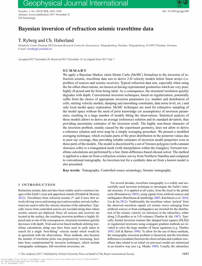
Figure 1. Sketch showing different tomographic scenarios depending ondistribution of sources and receivers, colour coded according to ray density(a proxy to potential tomographic spatial resolution). Top: ‘Scenario A’is representative of tomographic geometries with ‘good’ distribution ofreceivers and/or sources yielding even ray coverage with many crossing raysand—in turn—resulting in a compact region of good resolution (white). Thetransition region (light red) at the border to the unresolved region (red) israther small. This scenario is typically found in studies of ambient noisederived group velocities of Rayleigh waves, medical computer tomographicscenarios (MRT) and—roughly—also in cross-hole seismic tomography.Bottom: ‘Scenario B’ depicts the ray distribution of a typical refraction styledata set with sources and receivers situated along a line at the surface. Thisgeometry is characterized by a rather small well-resolved region directlybelow the surface (white) and a wide gradual transition (light red) towardthe unresolved deeper regions (red). Note many subparallel ray paths andonly a few crossing rays in the deeper parts captured only by the far-offsetrecordings. Note that the ray paths for individual models investigated alongthe Markov chain, while still fitting the data very well, will significantlydiffer from the distribution shown here.

Sambridge 2009). For this inversion technique, the ‘final’ inversionresult (reference solution) is derived by a superposition (averaging)of a large number of well-fitting models.

A natural extension of this approach treats the omnipresent dataerror (sometimes difficult to be quantified) as an extra, unknownvariable, and consequently inverts for this parameter (Bodin et al.2012a). For these so-called Hierarchical Bayes methods (Bodinet al. 2012a), the level of data noise (data uncertainty, i.e. typicaltraveltime data errors and forward modeling errors) directly affectsthe level of complexity (model dimension), that is, the inversion‘tries’ to decompose the data into a part needed to explain themodel and a residual one (actual noise or data uncertainty).

The transdimensional hierarchical tomography using Markovchain MC methods (McMC) has been successfully applied to2-D traveltime tomographic data sets situated in the horizontalplane, see Fig. 1, as for example ambient noise derived group ve-locity analysis of Rayleigh waves (see e.g. Bodin & Sambridge

Downloaded from https://academic.oup.com/gji/article-abstract/212/3/1645/4644833by Geoforschungszentrum Potsdam useron 22 December 2017

Refraction seismic traveltime data 1647

0

2

4

6

8

10

Tra

velti

me−

offs

et/8

[s]

−200 −150 −100 −50 0 50 100 150 200Model distance [km]

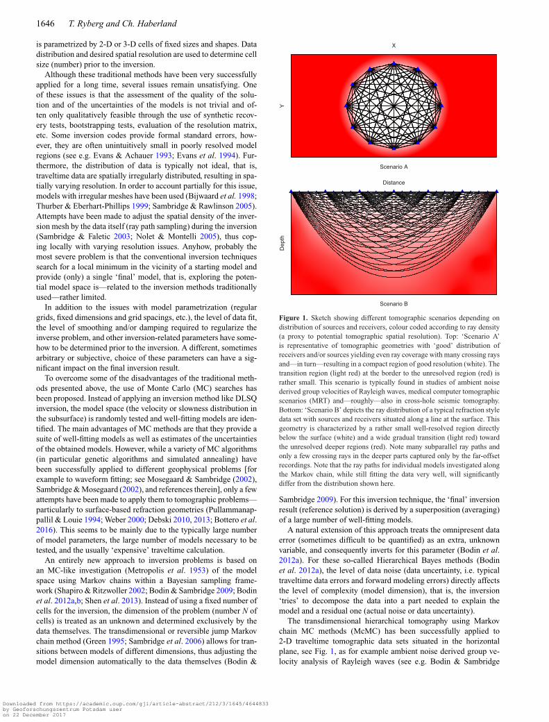
Figure 2. Reduced traveltime picks (black dots) for the real data set of Ryberg et al. (2015) for all 14 shots (red stars). All traveltime picks (1014) representP-wave first arrivals (refracted phases).

2009; Bodin et al. 2012b), to derive pseudo-3-D models (see e.g.Young et al. 2013a,b) or applied to true 3-D problems (see e.g.Hawkins & Sambridge 2015; Burdick & Lekic 2017). In the fol-lowing, we name this type of experiment geometry ‘Scenario A’(see also Fig. 1, top). Agostinetti et al. (2015) applied it to a lo-cal earthquake tomography problem. In this paper, we apply andextend the McMC inversion technique to 2-D controlled source,refraction style (wide-angle) seismic traveltime data to derive the2-D velocity distribution in the subsurface (along vertically orientedcross-sections). 2-D refraction style data sets consist of traveltimesof first arrivals recorded from several shots along a line of seismicreceivers (typically a larger number). All sources and receivers arelocated at the Earth’s surface and are distributed along a line. Thefirst arrivals are associated to refracted or diving phases resemblingarcuate rays whose course and depth penetration is critically con-trolled by the 2-D velocity distribution, primarily by the prevailingvertical velocity gradient. Fig. 1 (bottom) shows the general setupof this specific experiment geometry, in the following named ‘Sce-nario B’. This tomographic problem is especially ill-posed, giventhe unfavourable distribution of sources and receivers. Typically,only the very shallow region below the sources and receivers iswell constrained by data (traveltimes), while in the deeper part ofthe model ‘crossing’ rays are more or less absent, thus significantlyreducing the resolution power at depth. In ‘Scenario A’ experimentgeometries, the model space is roughly split into regions with rayspassing through and regions with no ray coverage (not constrainedby any data), and transitional regions in-between are rather small.In ‘Scenario B’ experiment geometries (refraction style data), mostof the inversion space is of intermediate character, with varying,but generally smaller numbers of rays passing through (see Fig. 1,bottom).

2 E X P E R I M E N TA L S E T U P A N D F I E L DDATA S E T

In this paper, we present an inversion method and its applicationto a typical, real refraction data set along from an onshore seis-mic refraction experiment at the eastern prolongation of the Walvis

Ridge into Africa. This seismic experiment, which was carried outin 2010/2011 and aimed to study the continental break-up and cre-ation of the South Atlantic ocean, consisted of a 320 km long, coast-parallel refraction profile in Northern Namibia. For the experimentshots from 14 boreholes were used as seismic sources. The explo-sions were recorded along the profile with 100 autonomous seismicdata loggers recording at 100 sps (samples per second) using short-period (4.5 Hz eigenfrequency), vertical component geophones (seeRyberg et al. 2015 for details). Fig. 2 shows the traveltime picks ofthe refracted P phases used in this study.

3 M O D E L PA R A M E T R I Z AT I O N

The 2-D models are described by a set of unstructured points pi = (xi,zi, vi) with 0 < i < N, located in the x–z plane (N is number of modelnodes; x is horizontal coordinate; z is depth and v is seismic velocityor slowness). For the interpolation between these model points (i.e.to generate a fine grid/mesh to calculate traveltimes), we follow andevaluate two approaches, one based on Voronoi cells (with constantvelocities within the cell), and one based on a triangulated mesh(with constant gradients within the cells).

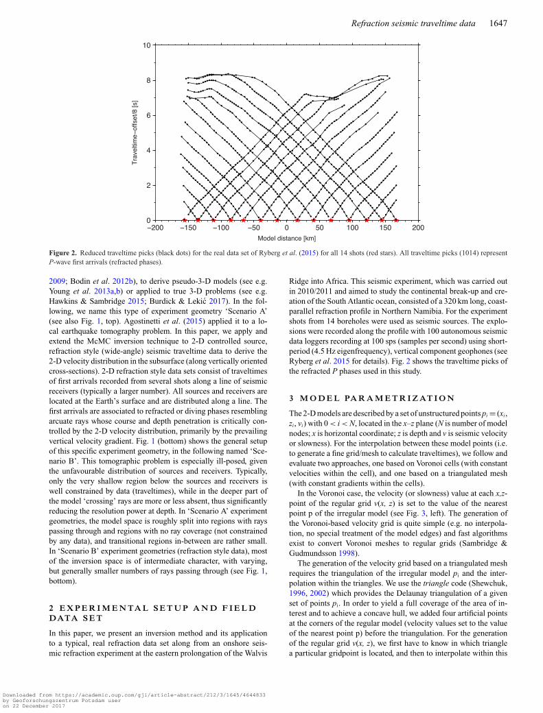
In the Voronoi case, the velocity (or slowness) value at each x,z-point of the regular grid v(x, z) is set to the value of the nearestpoint p of the irregular model (see Fig. 3, left). The generation ofthe Voronoi-based velocity grid is quite simple (e.g. no interpola-tion, no special treatment of the model edges) and fast algorithmsexist to convert Voronoi meshes to regular grids (Sambridge &Gudmundsson 1998).

The generation of the velocity grid based on a triangulated meshrequires the triangulation of the irregular model pi and the inter-polation within the triangles. We use the triangle code (Shewchuk,1996, 2002) which provides the Delaunay triangulation of a givenset of points pi. In order to yield a full coverage of the area of in-terest and to achieve a concave hull, we added four artificial pointsat the corners of the regular model (velocity values set to the valueof the nearest point p) before the triangulation. For the generationof the regular grid v(x, z), we first have to know in which trianglea particular gridpoint is located, and then to interpolate within this

Downloaded from https://academic.oup.com/gji/article-abstract/212/3/1645/4644833by Geoforschungszentrum Potsdam useron 22 December 2017

1648 T. Ryberg and Ch. Haberland

Figure 3. Examples for a Voronoi tesselation model (with constant slowness cells; left) and triangulated mesh (with interpolation within triangles; right) forthe same set of model points (black circles). Note the absence of sharp slowness contrasts in the triangulated mesh model.

triangle. The efficient search of the encircling triangle is performedby the walking triangle or trifind algorithm (Lawson 1977; Lee &Schachter 1980; Sambridge et al. 1995) without the need to checkall triangles. The interpolation within a particular triangle is done bybarycentric interpolation well known from computer graphics (e.g.Mobius 1827). Fig. 3 (right) shows the velocity distribution basedon the triangulation. Using these two methods (either Voronoi-cell-based or triangulation-based) fine and regular 2-D-grids/meshes areefficiently generated from the unstructured point models pi.

4 F O RWA R D P RO B L E M

The resulting regular grid (either based on Voronoi constant slow-ness cells or on triangulated mesh and interpolation, see above)is then used in a finite-difference (FD) eikonal solver (Podvin &Lecomte 1991) to calculate the first arrival traveltimes for all sourceand receiver pairs. This traveltime estimation using an eikonal solveris very efficient and no ray tracing is needed. Since traveltimes arecalculated on a regular grid, bilinear interpolation between the encir-cling gridpoints is used to calculate the arrival times at the specificreceiver positions. Eventually, the root-mean-square (rms) valueof the differences between the measured and calculated traveltimevalues of a particular model is estimated.

For our applications to synthetic and real data, we used a gridspacing (in x- and z-directions) of 1 km, resulting in FD grids of320 × 80 in size. We extensively tested the potential influence ofthe forward grid size by using sparser and finer grids. We foundno significant differences between the derived reference models forforward grid sizes of 0.25, 0.5, 1.0, 2.0 and 4 km other than those in-troduced by the per se randomness of the MC technique. Even whenusing a sparse 4 km forward grid, were we would expect forwardtraveltime errors caused by the sparse model parametrization whenusing the eikonal solver, a reference model which did not differfrom those with finer forward grids could be inverted for. To avoidpropagation (and eventually inversion) of waves above the Earth’ssurface, we replaced the gridded model above the surface by lowvelocities (Vair) before calculating traveltimes.

5 H I E R A RC H I C A L B AY E S I A NA P P ROA C H

We mainly follow the hierarchical transdimensional Bayes algo-rithm proposed by Bodin et al. (2012a,b) by studying multiple, non-interacting Markov chains. We start the Markov chains by choosinga randomly initialized model, then iteratively proceeding with theevolution algorithm. Every step of the Markov chain involves thefollowing steps: we propose a new model based on the currentmodel by (1) changing (with a probability of 1/5) the slowness of arandomly picked cell, or (2) changing the position (move) of a cell,

(3) changing the noise parameter, or (4) adding a new cell (birth) or(5) deleting a randomly chosen cell (death). The choice of the newvalues for the first three steps is based on the values for the currentmodel (position, slowness, or data noise) which are changed accord-ingly to a Gaussian probability distribution centred at the currentvalue. The Gaussian probability distributions are characterized byappropriate standard deviations sx and sz, ss and sn for horizontaland vertical moves, cell slowness and data noise, respectively. Wedid not allow cells to move outside the model boundaries and re-stricted the slowness values to be within smin and smax. Note thatthese values should be chosen carefully, so that the posterior dis-tribution will not be truncated by these limits. We assume minimalprior knowledge and a ‘nearly’ uninformative prior by choosing auniform prior distribution with relatively wide bounds (i.e. Bodinet al. 2012b; Shen et al. 2013; Young et al. 2013a,b; Pachai et al.2014). More details regarding the implementation of the Markovchains can be found in Bodin et al. (2012a).

Traveltimes are estimated for a newly proposed model (see above,Sections 3 and 4), then the misfit is used to determine the likelihoodof the new model. According to the acceptance criterion of Bodin &Sambridge (2009) or Moosegard & Tarantola (1995), the new modelis randomly accepted or rejected. To improve the acceptance rateand model space sampling we used the delayed rejection technique(DR; Tierney & Mira 1999; Mira 2001). The proposed new model(or retained current one in the case of rejection) then acts as astarting model for the next iteration. By reiterating this step, weproduce a chain of models (Markov chain). The first part of thischain (burn-in phase) is discarded until stationarity of random modelspace sampling is achieved. After this period, the chain of modelsis asymptotically distributed according to the posterior distribution,thus realizing a Metropolis sampling algorithm (Gallagher et al.2009).

6 R E F E R E N C E S O LU T I O N A N D E R RO RM A P

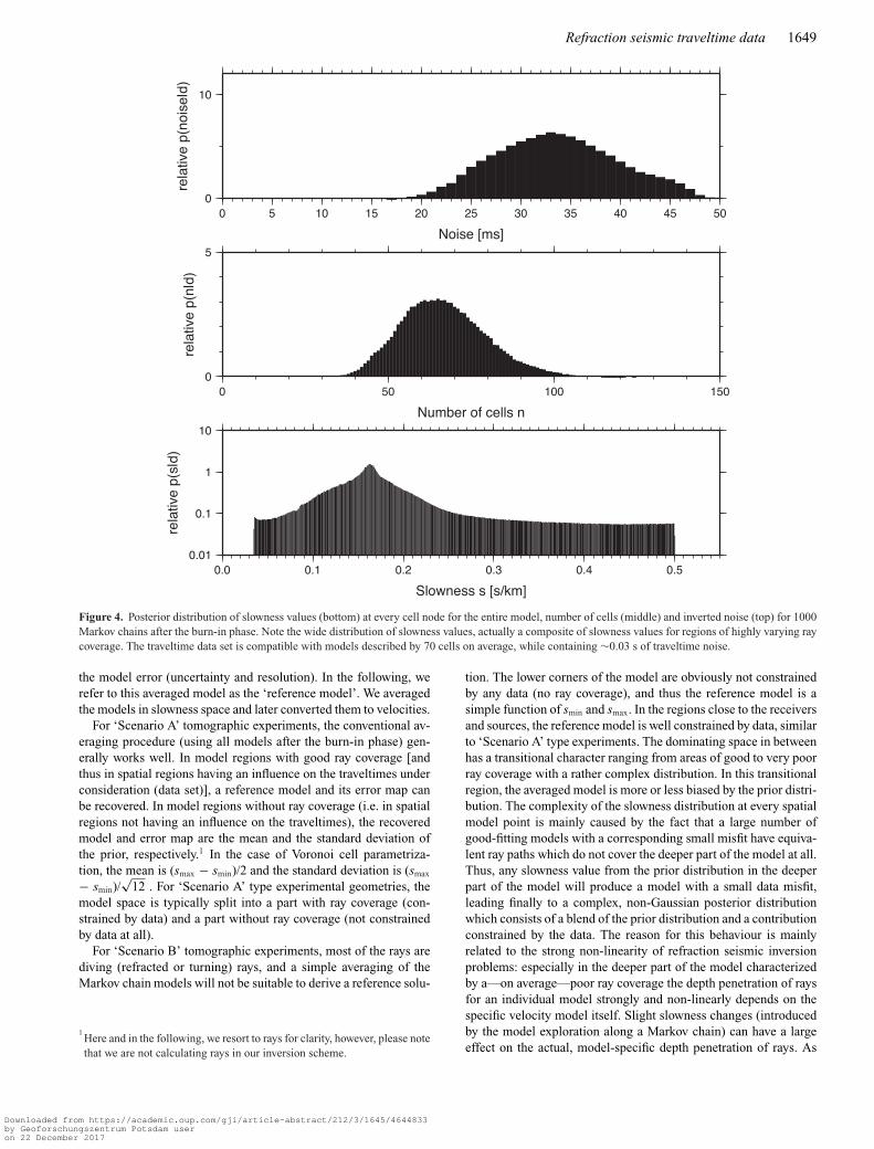
As the result of the Markov chain calculation, a large number ofmodels fitting the data set well are generated. Each such individ-ual model is usually coarse and looks very ‘ungeological’—generalexamples of these models are for example presented in Fig. 3.Fig. 4 shows the distribution of posterior values for the slowness,the number of cells and the inverted data noise of the well-fittingmodels (in the post burn-in phase).These models can be convertedinto a regular grid with a grid-specific spacing (see Section 3).From these gridded models, statistical properties like the average,standard deviation, median, etc., can be constructed locally at ev-ery model position (following Bodin & Sambridge 2009; Bodin etal. 2012a; Young et al. 2013a,b; Burdick & Lekic 2017; Galettiet al. 2017). Typically, the average model is treated as the referencesolution and the standard deviation is interpreted as a measure of

Downloaded from https://academic.oup.com/gji/article-abstract/212/3/1645/4644833by Geoforschungszentrum Potsdam useron 22 December 2017

Refraction seismic traveltime data 1649

0.01

0.1

1

10

rela

tive

p(s|

d)

0.0 0.1 0.2 0.3 0.4 0.5

Slowness s [s/km]

0

5

rela

tive

p(n|

d)

0 50 100 150

Number of cells n

0

10

rela

tive

p(no

ise|

d)

0 5 10 15 20 25 30 35 40 45 50

Noise [ms]

Figure 4. Posterior distribution of slowness values (bottom) at every cell node for the entire model, number of cells (middle) and inverted noise (top) for 1000Markov chains after the burn-in phase. Note the wide distribution of slowness values, actually a composite of slowness values for regions of highly varying raycoverage. The traveltime data set is compatible with models described by 70 cells on average, while containing ∼0.03 s of traveltime noise.

the model error (uncertainty and resolution). In the following, werefer to this averaged model as the ‘reference model’. We averagedthe models in slowness space and later converted them to velocities.

For ‘Scenario A’ tomographic experiments, the conventional av-eraging procedure (using all models after the burn-in phase) gen-erally works well. In model regions with good ray coverage [andthus in spatial regions having an influence on the traveltimes underconsideration (data set)], a reference model and its error map canbe recovered. In model regions without ray coverage (i.e. in spatialregions not having an influence on the traveltimes), the recoveredmodel and error map are the mean and the standard deviation ofthe prior, respectively.1 In the case of Voronoi cell parametriza-tion, the mean is (smax − smin)/2 and the standard deviation is (smax

− smin)/√

12 . For ‘Scenario A’ type experimental geometries, themodel space is typically split into a part with ray coverage (con-strained by data) and a part without ray coverage (not constrainedby data at all).

For ‘Scenario B’ tomographic experiments, most of the rays arediving (refracted or turning) rays, and a simple averaging of theMarkov chain models will not be suitable to derive a reference solu-

1Here and in the following, we resort to rays for clarity, however, please notethat we are not calculating rays in our inversion scheme.

tion. The lower corners of the model are obviously not constrainedby any data (no ray coverage), and thus the reference model is asimple function of smin and smax. In the regions close to the receiversand sources, the reference model is well constrained by data, similarto ‘Scenario A’ type experiments. The dominating space in betweenhas a transitional character ranging from areas of good to very poorray coverage with a rather complex distribution. In this transitionalregion, the averaged model is more or less biased by the prior distri-bution. The complexity of the slowness distribution at every spatialmodel point is mainly caused by the fact that a large number ofgood-fitting models with a corresponding small misfit have equiva-lent ray paths which do not cover the deeper part of the model at all.Thus, any slowness value from the prior distribution in the deeperpart of the model will produce a model with a small data misfit,leading finally to a complex, non-Gaussian posterior distributionwhich consists of a blend of the prior distribution and a contributionconstrained by the data. The reason for this behaviour is mainlyrelated to the strong non-linearity of refraction seismic inversionproblems: especially in the deeper part of the model characterizedby a—on average—poor ray coverage the depth penetration of raysfor an individual model strongly and non-linearly depends on thespecific velocity model itself. Slight slowness changes (introducedby the model exploration along a Markov chain) can have a largeeffect on the actual, model-specific depth penetration of rays. As

Downloaded from https://academic.oup.com/gji/article-abstract/212/3/1645/4644833by Geoforschungszentrum Potsdam useron 22 December 2017

1650 T. Ryberg and Ch. Haberland

1000

2000

3000

4000

His

togr

am c

ount

0.0 0.1 0.2 0.3 0.4 0.5

Slowness [s/km]

1000

2000

3000

4000

His

togr

am c

ount

0.0 0.1 0.2 0.3 0.4 0.5

Slowness [s/km]

x=150 kmz=60 km

5000

10000

15000

20000

His

togr

am c

ount

5000

10000

15000

20000

His

togr

am c

ount

x=75 kmz=30 km

10000

20000

30000

40000

50000H

isto

gram

cou

nt

10000

20000

30000

40000

50000H

isto

gram

cou

ntx=0 kmz=0 km

0.0 0.1 0.2 0.3 0.4 0.5

Slowness [s/km]

0.0 0.1 0.2 0.3 0.4 0.5

Slowness [s/km]

x=150 kmz=60 km

x=75 kmz=30 km

x=0 kmz=0 km

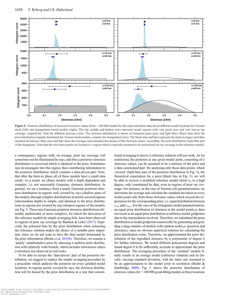
Figure 5. Posterior distribution of recovered slowness values (from ∼100 000 models for the same traveltime data set) at different model locations for Voronoimesh (left) and triangulation based models (right). The top, middle and bottom rows represent model regions with very good, poor and very low/no raycoverage, respectively. Note the different abscissa scales. The slowness distribution is shown as histogram plots (grey and light blue). Black lines show theprior distribution (equally distributed for Voronoi mesh models, complex for triangulated ones). The black stars and bars represent the plain averages (and theirstandard deviations). Blue stars and bars show the averages (and standard deviations) of the slowness values ‘exceeding’ the prior distribution (light blue partof the histogram). Note that the two lower panels are located in a region which is typically assumed to be unresolved (no ray coverage in the reference model).

a consequence, regions with, on average, poor ray coverage willsometimes not be illuminated by rays, and thus a posterior slownessdistribution is recovered which is identical to the prior. Sometimesrays do propagate into this region, thus contributing information tothe posterior distribution which contains a data-driven part. Note,that after the burn-in phase all of these models have a small datamisfit. As a result, we obtain models with a depth dependent andcomplex, i.e. not necessarily Gaussian, slowness distribution. Ingeneral, we see a tendency from a nearly Gaussian posterior slow-ness distribution in regions well covered by rays (shallow parts ofthe model), through complex distributions in poorly covered regions(intermediate depth) to simple, and identical to the prior distribu-tions in regions not covered by rays (deepest regions of the model),see Fig. 5. These non-Gaussian posterior slowness distributions (bi-modal, multimodal, or more complex), for which the derivation ofthe reference models by simple averaging fails, have been observedin regions of poor ray coverage by Burdick & Lekic (2017). Espe-cially the potential bias by the prior distribution when extractingthe reference solution makes the choice of a suitable prior impor-tant, since we do not want to have the final model dominated bythe prior information (Bodin et al. 2012b). Therefore, we assume a‘nearly’ uninformative prior by choosing a uniform prior distribu-tion with relatively wide bounds, which includes slownesses values(velocities) not observed in real rocks.

To be able to extract the ‘data-driven’ part of the posterior dis-tribution, we suggest to replace the simple averaging procedure bya procedure which analyses the posterior (at every gridded modellocation). In regions poorly covered by rays, the slowness distribu-tion will be biased by the prior distribution in a way that conven-

tional averaging to derive a reference solution will not work. As wementioned, the posterior at any given model point, consisting of nslowness values, can be assumed to be a mixture of the prior anda data constrained part. By analysing only those data points, which‘exceed’ (light blue part of the posterior distribution in Fig. 5), thetheoretical expectation for a prior (black line in Fig. 5), we willbe able to recover a modified reference model which is, to a highdegree, only constrained by data, even in regions of poor ray cov-erage. For instance, in the case of Voronoi cell parametrization, wedetermine the average and calculate the standard deviation at everymodel point only from those slowness values which exceed the ex-pectation for the corresponding prior, i.e. equal distribution betweensmin and smax. For the case of the triangulate model parametrization,an equal prior distribution of slowness at the model points pi doesnot result in an equal prior distribution at arbitrary model gridpointsdue to the interpolation involved. Therefore, we calculated the priordistribution at model gridpoints numerically by generating and grid-ding a large number of models with random nodes pi (position andslowness), since no obvious analytical solution for calculating theprior distribution exists. Therefore, we approximated the prior dis-tribution of the regridded slowness by a polynomial of degree 8for further reference. We tested different polynomial degrees andfound degree 8 to be sufficiently accurate to approximate the priordistribution. The averaging procedure of the ‘residual’ models fi-nally results in an average model (reference solution) and its (lo-cally varying) standard deviation, with the latter one assumed tobe an approximation to the model error or resolution (Bodin &Sambridge 2009). Fig. 5 shows the posterior distribution ofslowness values for ∼100 000 good-fitting models at three locations

Downloaded from https://academic.oup.com/gji/article-abstract/212/3/1645/4644833by Geoforschungszentrum Potsdam useron 22 December 2017

Refraction seismic traveltime data 1651

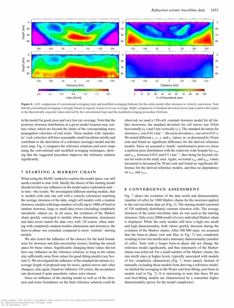
Figure 6. Left: comparison of conventional averaging (top) and modified averaging (bottom) for the entire model after slowness to velocity conversion. Notethat the conventional averaging is strongly biased in regions of poor to no ray coverage. Right: comparison of standard deviation (error map) scaled with respectto the theoretically expected values derived by the conventional (top) and the modified averaging procedure (bottom).

in the model for good, poor and very low ray coverage. Note that theposterior slowness distribution at a given model location may con-tain values which are beyond the limits of the corresponding wavepropagation velocities of real rocks. These models with ‘unrealis-tic’ rock velocities still have reasonably small traveltime misfits andcontribute to the derivation of a reference (average) model and theerror map. Fig. 6 compares the reference solutions and error mapsusing the conventional and modified averaging techniques, show-ing that the suggested procedure improves the reference solutionsignificantly.

7 S TA RT I N G A M A R KOV C H A I N

When using the McMC method to explore the model space, one stillneeds a model to start with. Ideally the choice of this starting modelshould not have any influence on the model space exploration and—in turn—the results. We investigated different starting models, thatis, models with only one cell with a velocity (slowness) matchingthe average slowness of the data, single cell models with a randomslowness, models with huge numbers of cells (up to 1000) of fixed orrandom slowness, large or small data errors (including completelyunrealistic values) etc. In all cases, the evolution of the Markovchain quickly converged to models whose dimension, slownessesand data errors match the data very well. Of course, when start-ing with completely random models (dimension and slowness), theburn-in phase was extended, compared to more ‘realistic’ startingmodels.

We also tested the influence of the choices for the hard bound-aries for slowness and data uncertainty (noise), limiting the searchspace for those values. Significantly changing those values did nothave any influence on the reference solution, as long as the valuesstay sufficiently away from values for good-fitting models (see Sec-tion 5). We investigated the influence of the standard deviations (i.e.average length of proposed step for noise, spatial moves and valuechanges), and, again, found no influence. Of course, the acceptancerate decreased if quite unrealistic values were chosen.

Since no influence of the starting model as well as of the slow-ness and noise boundaries on the final reference solution could be

observed, we used a 150-cell, constant slowness model for all fur-ther inversions, the standard deviation for cell moves was 10 kmhorizontally (sx) and 5 km vertically (sz). The standard deviation forslowness ss was 0.01 s km−1, the noise deviation sn was set to 0.01 s.We tested different sx , sz, ss and sn values, in- or decreased by 50 percent and found no significant difference for the derived referencemodels. Since we assumed a ‘nearly’ uninformative prior we chosea uniform prior distribution with the relatively wide bounds for smin

and smax between 0.035 and 0.5 s km−1, thus being far beyond val-ues for rocks in the study area. Again, we tested smin and smax valuesincreased or decreased by 50 per cent and found no significant dif-ference for the derived reference models, and thus no dependenceon smin and smax.

8 C O N V E RG E N C E A S S E S S M E N T

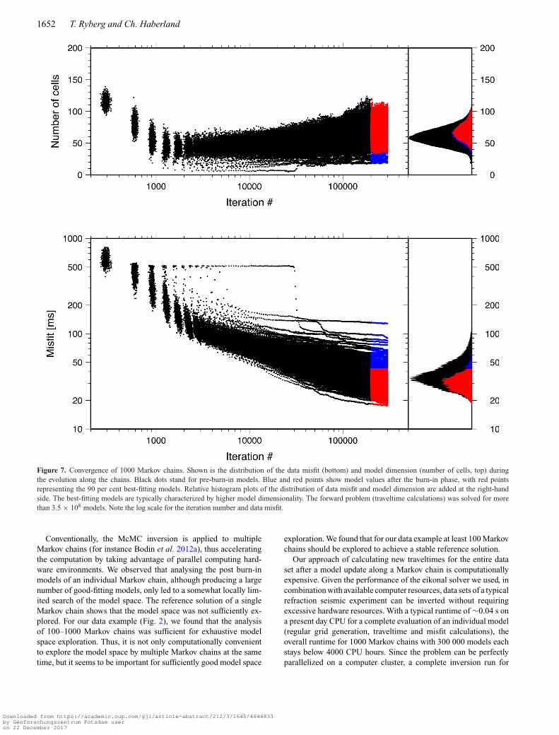
Fig. 7 shows the evolution of the data misfit and dimensionality(number of cells) for 1000 Markov chains for the inversion appliedto the real traveltime data set (Fig. 2). The starting model consistedof 150 randomly distributed, constant slowness cells. The averageslowness of the entire traveltime data set was used as the startingslowness. Only every 200th model of every individual Markov chainis displayed. While the early models still have a high rms misfitand high dimensionality, both values quickly decrease during theevolution of the Markov chains. After 200 000 steps, we assumedthat the burn-in phase (red and blue in Fig. 7) was completed,resulting in low rms misfits and a stationary dimensionality (numberof cells). Tests with a longer burn-in phase did not change thereference model significantly, and thus stationarity of the Markovchains was achieved. For a small number of the Markov chains, therms misfit stays at higher levels, typically associated with modelsof low complexity (dimension) (Fig. 7, lower panel). Instead ofmanually excluding those models from deriving a reference model,we limited the averaging to the 90 per cent best-fitting, post burn-inmodels (red in Fig. 7). It is interesting to note that these 90 percent best-fitting models are characterized by a somewhat higherdimensionality (proxy for the model complexity).

Downloaded from https://academic.oup.com/gji/article-abstract/212/3/1645/4644833by Geoforschungszentrum Potsdam useron 22 December 2017

1652 T. Ryberg and Ch. Haberland

Figure 7. Convergence of 1000 Markov chains. Shown is the distribution of the data misfit (bottom) and model dimension (number of cells, top) duringthe evolution along the chains. Black dots stand for pre-burn-in models. Blue and red points show model values after the burn-in phase, with red pointsrepresenting the 90 per cent best-fitting models. Relative histogram plots of the distribution of data misfit and model dimension are added at the right-handside. The best-fitting models are typically characterized by higher model dimensionality. The forward problem (traveltime calculations) was solved for morethan 3.5 × 108 models. Note the log scale for the iteration number and data misfit.

Conventionally, the McMC inversion is applied to multipleMarkov chains (for instance Bodin et al. 2012a), thus acceleratingthe computation by taking advantage of parallel computing hard-ware environments. We observed that analysing the post burn-inmodels of an individual Markov chain, although producing a largenumber of good-fitting models, only led to a somewhat locally lim-ited search of the model space. The reference solution of a singleMarkov chain shows that the model space was not sufficiently ex-plored. For our data example (Fig. 2), we found that the analysisof 100–1000 Markov chains was sufficient for exhaustive modelspace exploration. Thus, it is not only computationally convenientto explore the model space by multiple Markov chains at the sametime, but it seems to be important for sufficiently good model space

exploration. We found that for our data example at least 100 Markovchains should be explored to achieve a stable reference solution.

Our approach of calculating new traveltimes for the entire dataset after a model update along a Markov chain is computationallyexpensive. Given the performance of the eikonal solver we used, incombination with available computer resources, data sets of a typicalrefraction seismic experiment can be inverted without requiringexcessive hardware resources. With a typical runtime of ∼0.04 s ona present day CPU for a complete evaluation of an individual model(regular grid generation, traveltime and misfit calculations), theoverall runtime for 1000 Markov chains with 300 000 models eachstays below 4000 CPU hours. Since the problem can be perfectlyparallelized on a computer cluster, a complete inversion run for

Downloaded from https://academic.oup.com/gji/article-abstract/212/3/1645/4644833by Geoforschungszentrum Potsdam useron 22 December 2017

Refraction seismic traveltime data 1653

0

20

40

60

Dep

th [k

m]

−150−100−50050100150

Distance [km]

5.0

5.5

6.0

6.5

7.0

7.5

8.0

<V

p> [k

m/s

]

0

20

40

60

Dep

th [k

m]

−150−100−500501001505.0

5.5

6.0

6.5

7.0

7.5

8.0

FA

ST

Vp

[km

/s]

0

20

40

60

Dep

th [k

m]

−150−100−500501001500.1

0.2

0.5

1.0

2.0

Vp

erro

r [k

m/s

]

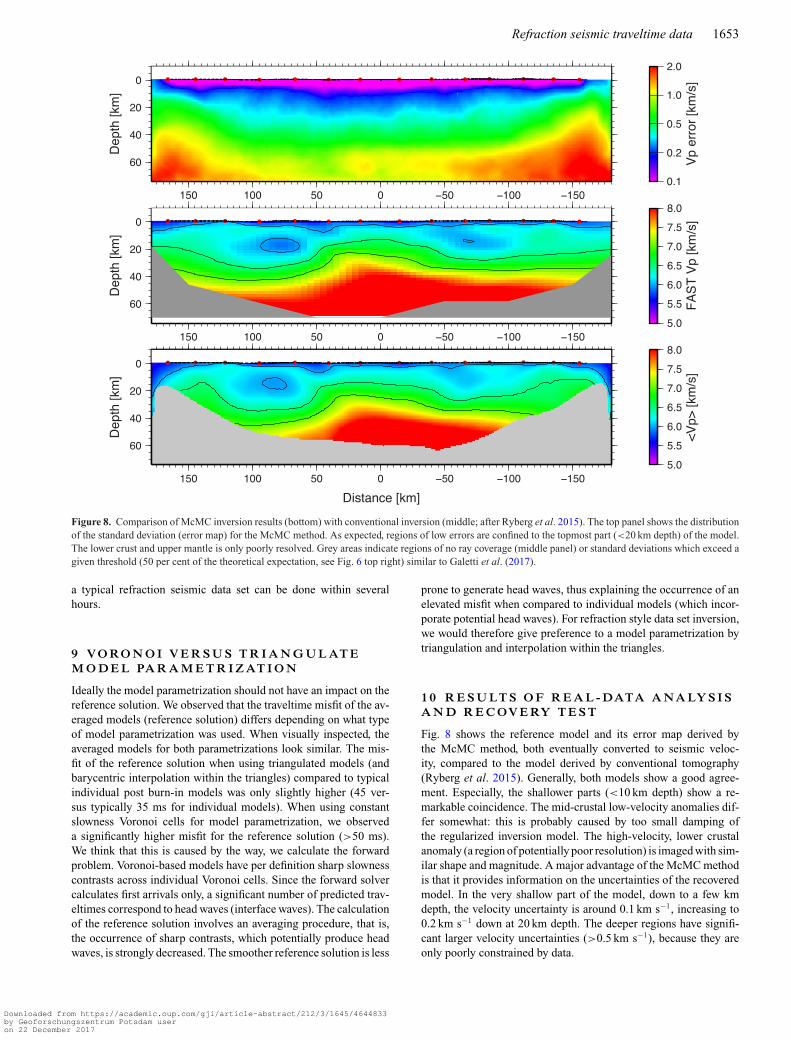
Figure 8. Comparison of McMC inversion results (bottom) with conventional inversion (middle; after Ryberg et al. 2015). The top panel shows the distributionof the standard deviation (error map) for the McMC method. As expected, regions of low errors are confined to the topmost part (<20 km depth) of the model.The lower crust and upper mantle is only poorly resolved. Grey areas indicate regions of no ray coverage (middle panel) or standard deviations which exceed agiven threshold (50 per cent of the theoretical expectation, see Fig. 6 top right) similar to Galetti et al. (2017).

a typical refraction seismic data set can be done within severalhours.

9 V O RO N O I V E R S U S T R I A N G U L AT EM O D E L PA R A M E T R I Z AT I O N

Ideally the model parametrization should not have an impact on thereference solution. We observed that the traveltime misfit of the av-eraged models (reference solution) differs depending on what typeof model parametrization was used. When visually inspected, theaveraged models for both parametrizations look similar. The mis-fit of the reference solution when using triangulated models (andbarycentric interpolation within the triangles) compared to typicalindividual post burn-in models was only slightly higher (45 ver-sus typically 35 ms for individual models). When using constantslowness Voronoi cells for model parametrization, we observeda significantly higher misfit for the reference solution (>50 ms).We think that this is caused by the way, we calculate the forwardproblem. Voronoi-based models have per definition sharp slownesscontrasts across individual Voronoi cells. Since the forward solvercalculates first arrivals only, a significant number of predicted trav-eltimes correspond to head waves (interface waves). The calculationof the reference solution involves an averaging procedure, that is,the occurrence of sharp contrasts, which potentially produce headwaves, is strongly decreased. The smoother reference solution is less

prone to generate head waves, thus explaining the occurrence of anelevated misfit when compared to individual models (which incor-porate potential head waves). For refraction style data set inversion,we would therefore give preference to a model parametrization bytriangulation and interpolation within the triangles.

1 0 R E S U LT S O F R E A L - DATA A NA LY S I SA N D R E C OV E RY T E S T

Fig. 8 shows the reference model and its error map derived bythe McMC method, both eventually converted to seismic veloc-ity, compared to the model derived by conventional tomography(Ryberg et al. 2015). Generally, both models show a good agree-ment. Especially, the shallower parts (<10 km depth) show a re-markable coincidence. The mid-crustal low-velocity anomalies dif-fer somewhat: this is probably caused by too small damping ofthe regularized inversion model. The high-velocity, lower crustalanomaly (a region of potentially poor resolution) is imaged with sim-ilar shape and magnitude. A major advantage of the McMC methodis that it provides information on the uncertainties of the recoveredmodel. In the very shallow part of the model, down to a few kmdepth, the velocity uncertainty is around 0.1 km s−1, increasing to0.2 km s−1 down at 20 km depth. The deeper regions have signifi-cant larger velocity uncertainties (>0.5 km s−1), because they areonly poorly constrained by data.

Downloaded from https://academic.oup.com/gji/article-abstract/212/3/1645/4644833by Geoforschungszentrum Potsdam useron 22 December 2017

1654 T. Ryberg and Ch. Haberland

0

20

40

60

Dep

th [k

m]

−150−100−50050100150

Distance [km]

5.0

5.5

6.0

6.5

7.0

7.5

8.0

Vp

[km

/s]

0

20

40

60

Dep

th [k

m]

−150−100−500501001505.0

5.5

6.0

6.5

7.0

7.5

8.0

<V

p> [k

m/s

]

0

20

40

60

Dep

th [k

m]

−150−100−50050100150

2

−10−8−6−4−2

02468

10

% d

iff

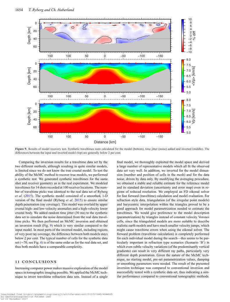
Figure 9. Results of model recovery test. Synthetic traveltimes were calculated for the model (bottom), time jitter (noise) added and inverted (middle). Thedifferences between the input and inverted model (top) are generally below 2 per cent.

Comparing the inversion results for a traveltime data set by thetwo different methods, although resulting in quite similar models,is limited since we do not know the true crustal model. To test theability of the McMC method to recover true models, we performeda synthetic test. We generated synthetic traveltimes for the sameshot and receiver geometry as in the real experiment. We modeledtraveltimes for 14 shots recorded at 100 receiver locations. The num-ber of traveltime picks was identical to the real data set of Ryberget al. (2015). The synthetic model consisted of a smoothed, 1-Dversion of the final model (Ryberg et al. 2015) to ensure similardepth penetration (ray coverage). This model was overlaid by uppercrustal high- and low-velocity anomalies and a high-velocity lowercrustal body. We added random time jitter (30 ms) to the syntheticdata set to simulate the noise determined from the real data travel-time picks. We then performed an McMC inversion and obtainedan inversion result (Fig. 9) which is very similar compared to theinput model. In most parts of the inverted model, including regionsof very poor ray coverage, the difference between both models staysbelow 2 per cent. The typical number of cells for the synthetic dataset (∼70, see Fig. 4) is of the same order as for the real data set, andthus both models have a comparable complexity.

1 1 C O N C LU S I O N S

Increasing computer power makes massive exploration of the modelspace in tomographic imaging possible. We applied the McMC tech-nique to invert traveltime refraction data sets. Instead of a single

final model, we thoroughly exploited the model space and deriveda large number of representative models which all fit the observeddata set very well. In addition, we inverted for the model dimen-sion (number and position of cells in the mesh) and for the datanoise, driven by data only. By modifying the averaging procedure,we obtained a stable and reliable estimate for the reference modeland its standard deviation (uncertainty and error map) even in re-gions of reduced resolution. We employed an FD eikonal solverfor fast forward (traveltime) calculation and model evaluation. Forrefraction style data, triangulation (of the irregular point models)and barycentric interpolation within the triangles proved to be agood approach for model parametrization needed to estimate thetraveltimes. We would give preference to the model description(parametrization) by triangles instead of constant velocity Voronoicells, since the triangulated models are more suitable to describerealistic earth models and have much smaller velocity jumps, whichmight cause traveltime errors when using the eikonal solver. Theforward problem (traveltime calculation) is completely performedfor each individual model during the search—this seems to be par-ticularly important in refraction type scenarios (Scenario ‘B’) inwhich even subtle velocity variations (of the predominantly verticalgradients) can result in very different ray paths, particularly verydifferent depth penetration. Given the nature of the McMC tech-nique, no starting model, pre-set parametrization values, dampingor smoothing parameters were needed. The result of the presentedinversion technique was compared to conventional inversion andsuccessfully tested with a synthetic data set, thus indicating a sim-ilar performance compared to conventional tomographic methods.

Downloaded from https://academic.oup.com/gji/article-abstract/212/3/1645/4644833by Geoforschungszentrum Potsdam useron 22 December 2017

Refraction seismic traveltime data 1655

However, the main advantage of the McMC approach is that it freesone from the choice of sometimes subjective and/or arbitrary param-eters used in conventional inversion techniques (inversion grid size,damping, smoothing, pre-set data noise, starting model, etc.), whileproviding important additional model constraints (error maps) andinformation on data noise. It would be straightforward to extendthe algorithm to the 3-D case, apply it to local earthquake data orcross-hole tomographic scenarios, invert for other hyperparameters(i.e. forward grid size) or include other data sets (i.e. S-wave travel-times, traveltimes of reflected phases, etc.) for joint inversions. Themethod can easily be adapted to different scales and performs wellwith multiscale problems.

A C K N OW L E D G E M E N T S

Instruments were provided by the Geophysical InstrumentPool Potsdam (GIPP) instrument pool of the DeutschesGeo-ForschungsZentrum GFZ Potsdam. Figures were prepared using theGeneric Mapping Tool GMT (Wessel & Smith 1995, 1998). Theauthors gratefully acknowledge the comments of the two anony-mous reviewers and Jim Mechie that helped to improve this paper.We thank Jonathan Richard Shewchuk for making his triangle rou-tine available. We thank Thomas Bodin and FrederikTilmann foradvice and discussions on this study. Calculations were performedon the GFZ Linux Cluster.

R E F E R E N C E S

Agostinetti, N.P., Giacomuzzi, G. & Malinverno, A., 2015. Local three-dimensional earthquake tomography by transdimensional Monte Carlosampling, Geophys. J. Int., 201, 1598–1617.

Bijwaard, H., Spakman, W. & Engdahl, E.R., 1998. Closing the gap betweenregional and global travel time tomography, J. geophys. Res., 103(B12),30 055–30 078.

Bodin, T. & Sambridge, M., 2009. Seismic tomography with the reversiblejump algorithm, Geophys. J. Int., 178(3), 1411–1436.

Bodin, T., Sambridge, M., Rawlinson, N. & Arroucau, P., 2012a. Transdi-mensional tomography with unknown data noise, Geophys. J. Int., 189(3),1536–1556.

Bodin, T., Sambridge, M., Tkalcic, H., Arroucau, P., Gallagher, K. &Rawlinson, N., 2012b. Transdimensional inversion of receiver func-tions and surface wave dispersion, J. geophys. Res., 117, B02301,doi:10.1029/2011JB008560

Bottero, A., Gesret, A., Romary, Th., Noble, M. & Maisons, Ch., 2016.Stochastic seismic tomography by interacting Markov chains, Geophys.J. Int., 207(1), 374–392.

Burdick, S. & Lekic, V., 2017. Velocity variations and uncertainty fromtransdimensional P-wave tomography of North America, Geophys. J. Int.,209(2), 1337–1351.

Debski, W., 2010. Seismic tomography by Monte Carlo sampling, Pure appl.Geophys., 167(1–2), 131–152.

Debski, W., 2013. Bayesian approach to tomographic imaging of rock-massvelocity heterogeneities, Acta Geophys., 61(6), 1395–1436.

Evans, J.R. & Achauer, U., 1993. Teleseismic velocity tomography usingthe ACH method: theory and applications to continental-scale studies, inSeismic Tomography: Theory and Practice, pp. 319–360, eds Iyer, H.M.& Hirahara, K., Chapman and Hall.

Evans, J.R., Eberhart-Phillips, D. & Thurber, C.H., 1994. User’s manualfor SIMULps for imaging Vp and Vp/Vs: a derivative of the "Thurber"tomographic inversion SIMUL3 for local earthquakes and explosions.Open-File Rep., U.S. Geol. Surv. USGS-OFR-94-431.

Galetti, E., Curtis, A., Baptie, B., Jenkins, D. & Nicolson, H., 2017. Transdi-mensional Love-wave tomography of the British Isles and shear-velocitystructure of the East Irish Sea Basin from ambient-noise interferometry,Geophys. J. Int., 208(1), 36–58.

Gallagher, K, Charvin, K, Nielsen, S., Sambridge, M. & Stephen-son, J., 2009. Markov chain Monte Carlo (MCMC) sampling meth-ods to determine optimal models, model resolution and modelchoice for Earth Science problems, Mar. Petrol. Geol., 26(4), 525–535.

Green, P., 1995. Reversible jump Markov chain Monte Carlo computationand Bayesian model determination, Biometrika, 82(4), 711–732.

Hawkins, R. & Sambridge, M., 2015. Geophysical imaging using trans-dimensional trees, Geophys. J. Int., 203(2), 972–1000.

Lawson, C.L., 1977. Software for C1 Surface Interpolation, in MathematicalSoftware III, pp. 161–194, ed. Rice, J.R., Academic Press.

Lee, D.T. & Schachter, B.J., 1980. Two algorithms for constructing a Delau-nay triangulation, Int. J. Comput. Inform. Sci., 9(3), 219–242.

Liu, Q. & Gu, Y.J., 2012. Seismic imaging: from classical to adjoint tomog-raphy, Tectonophysics, 566, 31–66.

Menke, W., 1989. Geophysical Data Analysis: Discrete Inverse Theory,International Geophysics Series, Academic Press.

Metropolis, N., Rosenbluth, M.N., Rosenbluth, A.W., Teller, A.H. & Teller,E., 1953. Equation of state calculations by fast computing machines, J.Chem. Phys., 21(6), 1087–1092.

Mira, A., 2001. On Metropolis-Hastings algorithm with delayed rejection,Metron, LIX(3–4), 231–241.

Mobius, A.F., 1827. Der Barycentrische Calcul, Johann Ambrosius BarthVerlag.

Mosegaard, K. & Sambridge, M., 2002 Monte Carlo analysis of inverseproblems, Inverse Probl., 18(3), R29–R54.

Mosegaard, K. & Tarantola, A., 1995. Monte Carlo sampling of solutionsto inverse problems, J. geophys. Res., 100(B7), 12 431–12 447.

Nolet, G. & Montelli, R., 2005. Optimal parametrization of tomographicmodels, Geophys. J. Int., 161(2), 365–372.

Pachhai, S., Tkalcic, H. & Dettmer, J., 2014. Bayesian inference for ultralowvelocity zones in the Earth’s lowermost mantle: complex ULVZ beneaththe east of the Philippines, J. geophys. Res., 119, 8346–8365.

Podvin, P. & Lecomte, I., 1991. Finite difference computation of traveltimesin very contrasted velocity models: a massively parallel approach and itsassociated tools, Geophys. J. Int., 105(1), 271–284.

Prodehl, C. & Mooney, W.D., 2012. Exploring the Earth’s crust: history andresults of controlled-source seismology, Geol. Soc. Am. Mem., 208, 764,doi:10.1130/2012.2208(002).

Pullammanappallil, S.K. & Louie, J., 1994. A generalized simulated-annealing optimization for inversion of first-arrival times, Bull. seism.Soc. Am., 84(5), 1397–1409.

Rawlinson, N. & Sambridge, M., 2003. Seismic traveltime tomography ofthe crust and lithosphere, Adv. Geophys., 46, 81–198.

Rawlinson, N., Pozgay, S. & Fishwick, S., 2010. Seismic tomography:a window into deep Earth, Phys. Earth planet. Inter., 178(3–4), 101–135.

Romanowicz, B., 2003. Global mantle tomography: progress status in thepast 10 years, Annu. Rev. Earth Planet. Sci., 31(1), 303–328.

Ryberg, T., Haberland, C., Haberlau, T., Weber, M., Bauer, K., Behrmann,J.H. & Jokat, W., 2015. Crustal structure of northwest Namibia: evidencefor plume-rift-continent interaction, Geology, 43(8), 739–742.

Sambridge, M. & Gumundsson, O., 1998. Tomographic systems of equationswith irregular cells, J. geophys. Res., 103(B1), 773–781.

Sambridge, M. & Faletic, R., 2003. Adaptive whole Earth tomography,Geochem. Geophys. Geosyst., 4(3), 1022, doi:10.1029/2001GC000213.

Sambridge, M. & Mosegaard, K., 2002. Monte Carlo methodsin geophysical inverse problems, Rev. Geophys., 40(3), 1009,doi:10.1029/2000RG000089.

Sambridge, M. & Rawlinson, N., 2005. Seismic tomography with irregularmeshes, in Seismic Earth: Array Analysis of Broadband Seismograms,pp. 49–65, eds Levander, A. & Nolet, G. American Geophysical Union.

Sambridge, M., Braun, J. & McQueen, H., 1995. Geophysical parametriza-tion and interpolation of irregular data using natural neighbours, Geophys.J. Int., 122(3), 837–857.

Sambridge, M., Gallagher, K., Jackson, A. & Rickwood, P., 2006. Trans-dimensional inverse problems, model comparison and the evidence, Geo-phys. J. Int., 167(2), 528–542.

Downloaded from https://academic.oup.com/gji/article-abstract/212/3/1645/4644833by Geoforschungszentrum Potsdam useron 22 December 2017

1656 T. Ryberg and Ch. Haberland

Shapiro, N.M. & Ritzwoller, M.H., 2002. Monte-Carlo inversion for a globalshear-velocity model of the crust and upper mantle, Geophys. J. Int.,151(1), 88–105.

Shen, W., Ritzwoller, M.H., Schulte-Pelkum, V. & Lin, F.C., 2013. Jointinversion of surface wave dispersion and receiver functions: a BayesianMonte-Carlo approach, Geophys. J. Int., 192(2), 807–836.

Shewchuk, J.R., 1996. Triangle: engineering a 2D quality mesh generatorand delaunay triangulator, in Applied Computational Geometry: TowardsGeometric Engineering’, pp. 203–222, eds Lin, M.C. & Manocha, D.,Lecture Notes in Computer Science, Vol. 1148, Springer-Verlag.

Shewchuk, J.R., 2014. Reprint of: Delaunay refinement algorithms for tri-angular mesh generation, Comput. Geom., 47(7), 741–778.

Thurber, C.H., 1993. Local earthquake tomography: velocities and VP/VS-theory, in Seismic Tomography, pp. 563–583, eds Iyer, H.M. & Hirahara,K., Chapman and Hall.

Thurber, C.H. & Aki, K., 1987. Three-dimensional seismic imaging, Annu.Rev. Earth planet. Sci., 15(1), 115–139.

Thurber, C.H. & Eberhart-Phillips, D., 1999. Local earthquake tomographywith flexible gridding, Comput. Geosci., 25(7), 809–818.

Tierney, L. & Mira, A., 1999. Some adaptive Monte Carlo methods forBayesian inference, Stat. Med., 8(17–18), 2507–2515.

Weber, Z., 2000. Seismic traveltime tomography: a simulated annealingapproach, Phys. Earth planet. Inter., 119(1–2), 149–159.

Wessel, P. & Smith, W., 1995. New version of the generic mapping tools,EOS, Trans. Am. geophys. Un., 76(33), 329–329.

Wessel, P. & Smith, W., 1998. New, improved version of generic mappingtools released, EOS, Trans. Am. geophys. Un., 79(47), 579–579.

Young, M.K., Rawlinson, N. & Bodin, T., 2013a. Transdimensional inversionof ambient seismic noise for 3D shear velocity structure of the Tasmaniancrust, Geophysics, 78(3), WB49–WB62.

Young, M.K., Cayley, R.A., McLean, M.A., Rawlinson, N.,Arroucau, P. & Salmon, M., 2013b. Crustal Structure of the east Gond-wana margin in southeast Australia revealed by transdimensional am-bient seismic noise tomography, Geophys. Res. Lett., 40(16), 4266–4271.

Zelt, C. & Barton, P.J., 1998. Three-dimensional seismic refraction tomogra-phy: a comparison of two methods applied to data from the Faeroe Basin,J. geophys. Res., 103, 7187–7210.

Downloaded from https://academic.oup.com/gji/article-abstract/212/3/1645/4644833by Geoforschungszentrum Potsdam useron 22 December 2017