seismic inversion and the importance of low frequencies · seismic inversion and the importance of...

Seismic inversion and the importance of low frequencies


Kris Innanen and Gary Margrave

ABSTRACT

CREWES has made a significant effort this year to support seismic inversion by gener-ating (1) data rich in low frequencies (the Hussar experiment), and (2) model-based meth-ods to extend the spectra of bandlimited data. Here we provide in a tutorial setting illus-trations of the reasons why missing low frequencies have such a deleterious influence oninversion. After a brief review of inverse scattering and full waveform inversion, 1D exam-ples quickly expose the influence of low frequencies, as does an example synthesized fromHussar well-log data.

INTRODUCTION

In September of this year, CREWES undertook a broadband seismic experiment nearHussar, Alberta (see Margrave et al., 2011). The primary goal of the experiment was tosupport seismic inversion by providing data rich in low frequencies. Our purpose in thispaper is to present in a tutorial style some of the main reasons why low frequencies areneeded in inversion. The reasons are technical, but nevertheless quite accessible, and wecan expose them with very simple 1D scalar analytical and numerical examples.

REVIEW

Here we review some of the quantities used in inversion. If you want to get straight tothe results, this section can be skipped.

Waves and models

All seismic inversion methods involve (1) a background (or reference) medium, withinwhich we know how waves propagate, and (2) a perturbation, which expresses the differ-ence between this reference and the actual Earth beneath our feet. We begin with waveequations. In 1D, let the scalar wave equation that describes how waves actually propagatein the Earth be [

d2

dz2+

ω2

c2(z)

]︸︷︷︸actual wave operator

P (z, zs, ω)︸︷︷︸wave field in Earth

= δ(z − zs)︸︷︷︸source

.(1)

It has three main parts: (1) a wave operator, which contains the properties of the medium;(2) the wave field P which propagates in the medium; and (3) a source term, which we willtake to be a simple impulse located at zs. Next, consider a “modeling” wave equation, withthe right physics but with a reference medium, c0(z), that is distinct from c(z):[

d2

dz2+

ω2

c20(z)

]︸︷︷︸background medium

G(z, zs, ω)︸︷︷︸modelled wave field

= δ(z − zs). (2)

CREWES Research Report — Volume 23 (2011) 1

Innanen & Margrave

In the seismic inverse problem, an initial medium c0(z) is adjusted to be as close as possibleto c(z), through use of measurements of P .

Two approaches to this inverse problem have attained real stature in exploration seis-mology: inverse scattering and full waveform inversion. They are very different, but onething they have in common is that they both involve a breakup of the actual medium, c(z),into a part that agrees with the reference medium, and a difference term. We define s(z),or the “model”, the unknown in the seismic inverse problem, as follows:

s(z) =1

c2(z)=

1

c20(z)[1− α(z)]︸︷︷︸

inverse scattering

=1

c20(z)− α(z)

c20(z)= s0(z) + δs(z)︸︷︷︸

full waveform inversion

.(3)

Two slightly different ways of breaking up the model are shown. One appears explicitlyin terms of the reference scalar wavespeed model c0(z), and a dimensionless perturbationα(z). This breakup is typical of inverse scattering. The other makes use of the s notation,and involves a reference s0(z) and a difference term δs(z) in the same units. This breakupis typical of full waveform inversion.

The final quantity we wish to introduce at this stage is an exact, analytic form for themodeled Green’s function G, which holds for a homogeneous scalar wavespeed c0:

G(z, zs, ω) =eik|z−zs|

i2k(4)

where k = ω/c0, though any kn = ω/cn might be used.

Inverse scattering

The goal in inverse scattering is to develop formulas by which the perturbation α isdirectly calculated from measurements of P , given c0(z) and G. From PDE theory, if weknow the Green’s function for a wave operator like [·] in equation (2), then determining thefield for a more complicated source is easy: we multiply the source by the Green’s functionand integrate. We can use this trick to solve for P . Using equation (3), we replace c(z) inequation (1) with c0 and α, and then bring the α term to the right hand side:[

d2

dz2+ k2

0(z)

]P (z, zs, ω) = δ(z − zs) + k2

0(z)α(z)P (z, zs, ω). (5)

This is exactly what we need — a wave operator like the one in equation (2) and a morecomplicated source. P is determined now by multiplying it by G and integrating:

P (z, zs, ω) = G(z, zs, ω) +

∫dz′G(z, z′, ω)k2

0(z)α(z′)P (z′, zs, ω). (6)

We haven’t solved for P yet, since it is also under the integral on the right. But, this P canbe replaced by the whole right hand side, since the whole right hand side also equals P .

2 CREWES Research Report — Volume 23 (2011)


Doing this an infinite number of times we create the Born series

P (z,zs, ω) = G(z, zs, ω) +


0(z′)α(z′)G(z′, zs, ω)

+


0(z′)α(z′)

∫dz′′G(z′, z′′, ω)k2

0(z′′)α(z′′)G(z′′, zs, ω)

+ ... .

(7)

If we subtract G from both sides, and fix z and zs to be on some measurement surface,equation (7) becomes a model for our data D(ω) = P − G|measured. It can be directlyinverted as follows. We form the inverse series α(z) = α1(z) + α2(z) + ..., in which αn isdefined to be nth order in measurements of D(ω), and equate like orders. This produces asequence of equations:

D1(ω) =


0(z′)α1(z′)G(z′, zs, ω),

D2(ω) =


0(z′)α2(z′)G(z′, zs, ω),

...

(8)

etc., where D1 = D(ω),

D2 = −∫dz′G(z, z′, ω)k2

0(z′)α1(z′)

∫dz′′G(z′, z′′, ω)k2

0(z′′)α1(z′′)G(z′′, zs, ω), (9)

and so on, with the Dn becoming progressively more complicated functions of lower orderD’s as n grows. We can solve the first equation in (8) for α1(z), use α1(z) to make D2

using equation (9), put that into the second equation in (8), solve for α2(z), and continuethis process. Summing these up we eventually reconstruct the full α(z).

It has been recognized (Clayton and Stolt, 1981) that, at any stage in equation (8),something akin to migration is going on. Solving

D1(ω) =


0(z′)α1(z′)G(z′, zs, ω) (10)

for α1(z), for instance, involves inverting the operator∫G[·]G. The right G acts from

left to right, bringing the wave from the model point z′ at depth to the source zs. Theleft G acts from right to left, bringing the wave from the model point z′ to the receiverz. Stripping these off, to expose α1, undoes these two operations, effectively downwardcontinuing sources and receivers and applying an imaging condition simultaneously.

Full waveform inversion

We next go back to the start again and discuss the basic form for full waveform inver-sion, an iterative methodology in which modeled and measured fields are compared and theformer is updated. Recall we discuss two fields, P and G; here they signify

P (zg, zs, ω) : Field in actual medium, DATA = P |ms

G(zg, zs, ω|s(n)0 ) : Modeled field in current medium model iteration s(n)

0 .(11)


Innanen & Margrave

To compare them at a particular iteration, we take their difference to be δP :

δP (zg, zs, ω|s(n)0 ) ≡ P (zg, zs, ω)−G(zg, zs, ω|s(n)

0 ). (12)

The model is the wavespeed structure of the medium with which we calculate G. Wediscuss it in terms of s0. Our aim will be to take a current version of s0, and, by analyzingthe measured data, update it so that it after the update it is closer to the actual medium thanit was before. For our current purposes we envision the step:

s(n+1)0 (z) = s

(n)0 (z) + µ(n)g(n)(z), (13)

where µ is the step-length, and g is the “direction” of the step.

To discuss the direction g, we choose an objective-function which is (1) expressed interms of the medium model and our measured data, and (2) is (by assumption) small whenthe medium model is close to the actual model, and large when the medium model is farfrom the actual model. An objective function Φ which fits this bill is just the magnitude ofthe differences δP :

Φ ≡ 1

2

∫dω{|δP |2

}. (14)

The objective function is usefully thought of as a kind of landscape of hills and valleys,with a point on the landscape for every possible model. Where the model and the actualmedium are very different is “higher ground” on the landscape, since Φ has a greater valuethere. We say that we have solved the inverse problem when we have found the modelassociated with the lowest point on Φ — the bottom of the deepest valley, where the modeland the medium are maximally in agreement.

If a guess s0 lands us anywhere other than the lowest point on Φ, a good step to take,it would seem, is directly “downhill”: the same direction a ball would roll if we put it onthe landscape and let it go. That direction is the gradient of Φ. Let, then, g be the gradientof Φ taken with respect to each model parameter (i.e., s0(z) at each depth z). Skipping thealgebra, taking the derivative of equation (14) with respect to s0 we get the integral of theproduct of two terms:

g(n)(z) = −∫dωRe

{∂G(zg, zs, ω|s(n)

0 )

∂s(n)0 (z)

δP ∗(zg, zs, ω|s(n)0 )

}. (15)

By way of terminology, in equation (15) the quantities

∂G(zg, zs, ω|s(n)0 )

∂s(n)0 (z)

, and δP (zg, zs, ω|s(n)0 ), (16)

are referred to as the sensitivities (or Fréchet derivatives), and the data residuals respec-tively. A final bit of (skipped) algebra and we derive a form for the sensitivities that holdsfor wave-type problems:

∂G(zg, zs, ω|s(n)0 )

∂s(n)0 (z)

= −ω2G(zg, z, ω|s(n)0 )G(z, zs, ω|s(n)

0 ), (17)



in which case the gradient, or step direction to take away from our initial guess, is

g(n)(z) =

∫dωω2[G(z, zs, ω|s(n)

0 )]× [G(zg, z, ω|s(n)0 )δP ∗(zg, zs, ω|s(n)

0 )]. (18)

Remarkably (given how different this derivation is from that of inverse scattering), thisstep direction, the calculation of which is the engine of full waveform inversion, is alsoclosely related to migration. Evidently, at any given step, we take the residuals δP , timereverse them (via the ∗), backpropagate them from the receiver zg to a depth point z, via theG(zg, z, ω|s(n)

0 ) term, forward model a source wave field from zs to the same point z, viathe G(z, zs, ω|s(n)

0 ) term, and correlate them. This is equivalent to downward continuationof sources and receivers followed by the application of an imaging condition.

Expressing layers and steps mathematically

Later we will choose, as example models, sets of layers where each layer has a par-ticular velocity c. We will write down what reflection data from such a model will looklike, choose a simple background medium, and then see how full waveform inversion actsto re-create the layers. This will be a mathematical (but insightful!) exercise. So, to seewhether FWI is doing what it should, we will need to be able to recognize the layers whenthey appear, mathematically, in the results.

We will express layers as sums of functions H which each represent a single step, of acertain height at a certain place. These are called Heaviside functions, and are defined as

H(z) =

{0 z < 01 z > 0

. (19)

H(z) is the antiderivative of the delta function: H(z) =∫ z

−∞ δ(z′)dz′. So, since the inverse

Fourier transform of a delta function centred at z0 is

δ(z − z0) =1

2π

∫dkze

ikz(z−z0), (20)

by taking the antiderivative of both sides of equation (20), we obtain for the Heavisidefunction

H(z − z0) =1

2π

∫dkz

eikz(z−z0)

ikz

. (21)

Recognizing these will help interpreting the full waveform inversion examples to come.

INVERSE SCATTERING I: DATA SPECTRUM AND MODEL SPECTRUM

The easiest way to see how important low frequencies are to inversion, and where in thereconstructed model they make their presence known, is to examine the inverse scatteringproblem in the linear regime. That is, we take the first term in the Born series in equation(8), and, assuming the perturbation to be small, make the approximation α(z) ≈ α1(z), inwhich case we have the self contained relationship

D(ω) =


0(z′)α(z′)G(z′, zs, ω). (22)


Innanen & Margrave

Let us next assume a homogeneous reference medium with wavespeed c0, in which casewe may use the Green’s function in equation (4). Using the fact that in a reflection exper-iment z and zs, the receiver and source depths, are both less than the depth support of theperturbation (i.e., all the unknown structure is below our feet), we have

D(ω) =

∫dz′[eik0(z′−z)

i2k0

]k2

0α(z′)

[eik0(z′−zs)

i2k0

]=

k20

(i2k0)2e−ik0(z+zs)

∫dz′ei2k0z′

α(z′)

= A(ω)α̂

(−2

ω

c0

),

(23)

where in the last step we have (1) accumulated all the pre-factors intoA, and (2) recognizedthat the remaining parts of the Green’s functions, appearing under the integral, turn theintegral into a Fourier transform over depth. The α̂ are, then, the Fourier coefficients ofα. Inspecting the transform, we see that the factor −2ω/c0 is the Fourier dual of depth z.Hence, we may refer to it as kz, the depth wavenumber. We have in other words produceda simple relationship between data and model:

D(ω) ∝ α̂ (kz) . (24)

The inverse problem now could not be simpler: we take temporal frequencies from our data(D), and populate the spatial frequencies of the model (α̂). Once they are full populated,through an inverse Fourier transform we have a reconstruction of α(z).

Also clear is the influence of missing low frequencies. Since kz ∝ ω, a missing lowfrequency datum will translate to a similar missing low wavenumber datum; hence missinglow data frequencies will translate into missing low wavenumber, or smoothly varying,parts of the model.

A further important point (especially for the nonlinear parts of inverse scattering andthe higher order iterations of full waveform inversion): models that have been reconstructedwithout their low wavenumbers lose their ability to sustain structure in depth. A simplenumerical example will demonstrate. Suppose data from a two layer model are invertedusing equation (24). In Figure 1 the spectrum of these data are plotted three times (toprow), each time with more of the low frequency content having been removed. Below theconsequent linearized reconstructions α(z) are plotted in black, with the full bandwidthresults in blue for comparison.

The models with missing low frequency exhibit a characteristic “droop”. Considerthe bandlimited reconstruction of the shallowest interface in the bottom right panel. Aninterface is more or less discernible in the expected location, but the lower medium cannotsustain in depth the step in wavespeed. This problem, which inverse scattering sharesequally with full waveform inversion, will be seen to cause issues in nonlinear correctionsin the former case, and in iterative updating in the latter case.



−5 0 5−0.05

0

0.05

0.1

0.15

Frequency f (Hz)

0 500 1000−0.2

0

0.2

0.4

Pseudo−depth z (m)

−5 0 5−0.05

0

0.05

0.1

0.15

Frequency f (Hz)

0 500 1000−0.2

0

0.2

0.4


−5 0 5−0.05

0

0.05

0.1

0.15

Frequency f (Hz)

0 500 1000−0.2

0

0.2

0.4


FIG. 1. Linear inverse scattering reconstruction of a two-layer medium with progressive loss of lowfrequency content. Top row: data spectra; bottom row: linear reconstruction at full bandwidth (blue)and with low frequencies removed (black). Left column: 0 Hz missing; middle colum: 0-0.5 Hzmissing; right column: 0-1 Hz missing.

INVERSE SCATTERING II: PROPAGATION THROUGH THE PERTURBATION

In equation (24) and in Figure 1 the importance of low frequencies to linearized inver-sion is illustrated. Unfortunately, this importance only grows when nonlinear adjustment ofthe linear approximation is attempted. The correct construction of the data-like quantitiesDn in equation (8) turns out to be highly sensitive to bandwidth.

Let us see this by evaluating equation (9), that is, determining D2 in terms of the linearresult α1(z) pictured in Figure 1, and then inverting the Green’s operators to calculateα1(z). Substituting the homogeneous Green’s function in equation (4) into equation (9)and manipulating the result, we obtain

α2(z) = −1

2

d

dz

(α1(z)

∫ z

0

dz′α1(z′)

). (25)

Going further, we can select a subset of all the terms in the inverse series α1, α2, ..., andsum them, forming the nonlinear inverse approximation

αNL(z) ≈ 1

2π

∫dkz

∫dz′ exp

{−ikz

[z′ − 1

2

∫ z′

0

dz′′α1(z′′)

]}α1(z

′). (26)

The new inverse result is, given full bandwidth data, a closer approximation to α(z) thanwas the linear result (Innanen, 2008).

Equation (26) is a formula which, given a data trace, calculates the medium perturba-tions α(z) to a high degree of accuracy. How does it respond to missing low frequencies?


Innanen & Margrave

Notice that it — like all of the individual terms that make it up —involves the integral ofα1(z), which really means the integral of the data:

∫ z

0dz′α1(z

′). The purpose of integrat-ing in this way is, essentially, to drive inversion by expressing wave propagation through amedium other than the reference medium — through the perturbation. An analogy is theWKBJ approximation, in which a field has roughly the form

ψ ≈ exp

(iω

∫ z

0

dz′

c(z′)

), (27)

wherein the wave is given the correct phase by integrating through the medium c(z).

The integral of the full bandwidth signal (blue) and the bandlimited signal (black) inthe bottom right corner of Figure 1, whichever is being used, is the only thing that makesthe nonlinear output αNL(z) in equation (26) different from the linear input α1(z). If∫ z

0α1(z

′)dz′ → 0, then the two integrals become nested forward and inverse Fourier trans-forms, taking α1 to the Fourier domain and then back again, unchanged. But by eye, zerois exactly what the integral of the bandlimited signal will be. Bandlimitation will render allthe nonlinear work we have done irrelevant.

To summarize, for the nonlinear adjustments within inverse scattering to work, requiresthat the linear reconstruction allow notional waves to be calculated propagating through it.This is not possible with significantly bandlimited data.

FULL WAVEFORM INVERSION I: PROPAGATION THROUGH THE UPDATE

For all their differences, FWI and inverse scattering share in degree and kind this sen-sitivity to missing low frequencies. Let us see this next.

Full waveform inversion is not inherently analytical in nature, but rather occurs in itera-tive, usually highly numerical, steps. So, formulas like equation (26) are never determinedin FWI, and consequently we don’t have the same ability to analyze its behaviour. Wewill have to work a little harder to gain insight into the problem, by putting analytic datathrough one FWI iteration, and watching what gets made.

The models we will perform this exercise on are illustrated in Figures 2a–b. In Figure2a we illustrate a completely homogeneous medium with waves propagating with velocityc0 everywhere. This will serve as our background, or intial medium. It is the sort of startingmodel one would be forced to use with no prior knowledge of even the smooth backgroundvelocity of the Earth. In Figure 2b is a two-interface medium with three wave velocitiesc0, c1 and c2. We will pretend that this represents the actual Earth, and we will take a FWIiteration towards reconstructing it, given reflection data and the background medium asingredients.

In a single iteration of gradient-based FWI, the background model (which is homoge-neous in our case) will be adjusted by adding a scalar times the gradient of the objectivefunction. The scalar is generally determined by a line search. Here we will not worry aboutthe absolute scale of the correction, but instead its structure and relative amplitudes. So,



zg, zs = 0 z1 z2

c2

c1

c0

c0

(a)

(b)

FIG. 2. Models used for analytic calculation of a single FWI iteration. (a) Initial, or backgroundmedium, a homogeneous wholespace with velocity c0; (b) The “actual” medium, consisting of tworeflectors.

we can focus on the gradient alone. From equation (18) we have its form:

g(z) =

∫dωω2[G(z, 0, ω)]× [G(0, z, ω)δP ∗(0, 0, ω)]. (28)

To calculate g for one step, we evidently need to calculate three things: two modellingGreen’s functions for each point z in the medium, and the residuals, which are the differ-ences between the data and the modelled field for the fixed source and receiver point, whichwe will take to be zg = zs = 0.

The data in the “actual” medium (absent multiples) include the direct wave,G(0, 0, ω) =(i2k0)

−1, and reflections from the boundaries at depths z1 and z2. In the frequency domainthe data have the analytic form

D(ω) =1

i2k0

+R1ei2k0z1

i2k0

+R′2ei2k0z1

i2k0

ei2k1(z2−z1), (29)

where the two wavenumbers are k0 = ω/c0, k1 = ω/c1, and the two amplitudes are R1 =(c1 − c0)/(c1 + c0), R′2 = (1 − R2

1)R2, and R2 = (c2 − c1)/(c2 + c1). So, the complexconjugate of the residuals is

δP ∗(0, 0, ω) = [D(ω)−G(0, 0, ω)]∗

=

[1

i2k0

+R1ei2k0z1

i2k0

+R′2ei2k0z1

i2k0

ei2k1(z2−z1) − 1

i2k0

]∗= −R1

e−i2k0z1

i2k0

−R′2e−i2k0z1

i2k0

e−i2k1(z2−z1).

(30)


Innanen & Margrave

Since the two modelled fields are

G(z, 0, ω) = G(0, z, ω) =eik0z

i2k0

, (31)

the fully assembled gradient is given by

g(z) = −∫dωω2 ei2k0z

(i2k0)2

[R1e−i2k0z1

i2k0

+R′2e−i2k0z1

i2k0

e−i2k1(z2−z1)

]=R1c

20

4

∫dωei2k0(z−z1)

i2k0

+R′2c

20

4

∫dωei2k0(z−Z2)

i2k0

,

(32)

where

Z2 = z1 +k1

k0

(z2 − z1). (33)

To evaluate the two integrals, we replace dω with

dω =c02× d(2k0), (34)

such that

g(z) =R1c

30

8

∫d(2k0)

ei2k0(z−z1)

i2k0

+R′2c

30

8

∫d(2k0)

ei2k0(z−Z2)

i2k0

, (35)

which allows us to immediately write

g(z) =R1c

30π

4H(z − z1) +

R′2c30π

4H(z − Z2), (36)

having recognized the Fourier forms for step functions discussed in equation (21). Again,we will not put too much stock in the significance of the absolute amplitudes at the moment,but consider the relative amplitudes of the parts of g and its spatial structure. We canevidently say that

g(z) ∝ H(z − z1) +R′2R1

H(z − Z2), (37)

where, using the definitions of the wavenumbers and equation (33),

Z2 = z1 +c0c1

(z2 − z1). (38)

The first thing to say about what happens when we add the gradient in equation (37) to thereference medium, is that it is a big improvement. We go from a first guess, containing nointerfaces, to a second guess, containing the right number of interfaces (i.e., the two stepsH , one at z1 and one at Z2).

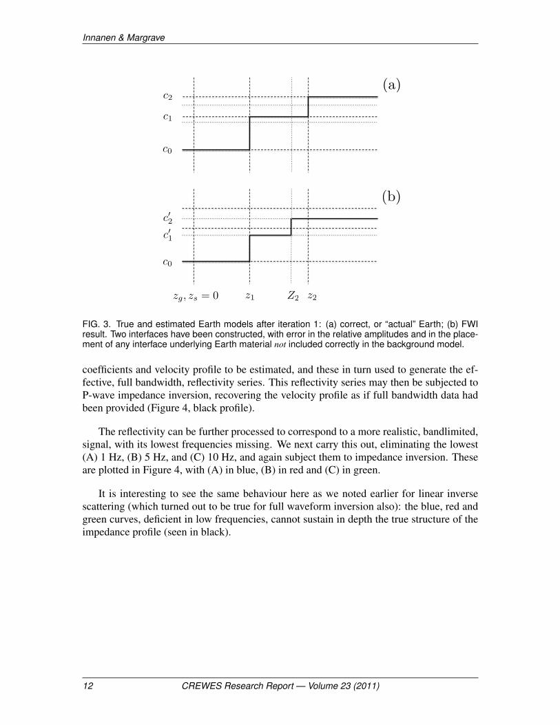
Equally clearly we have not achieved “the right answer”. We know that the correctdepth of the lower reflector is z2. We have misplaced it, putting it at Z2 6= z2. Also ingeneral the relative amplitude difference R′2/R1 is not precisely correct (see Figure 3).



To get at the issue of low frequency, we focus on the location of the lower interface.How wrong is it? By inspection of equation (38), the more c1 differs from c0, the morewrong Z2 is. Indeed, Z2 would equal z2 if c1 was equal to c0. The size of the placementerror, E, is proportional to the ratio (1− c0/c1):

E = |Z2 − z1| =(

1− c0c1

)|z1 − z2|. (39)

That makes sense. If the background medium velocity, i.e., our initial guess, was correct,all interfaces would be correctly placed—notice, for instance, the interface at z1 whichby chance was overlain by a medium that agrees with the background model, was placedcorrectly. This particular iteration only has c0 as a velocity to work with, even on dataevents whose history includes propagation at velocity c1, so some level of error was aninevitability.

The next iteration will know more, since the new medium (the one we will model innext time around) is the background plus the update, and the update knows about thesenew velocities. Well — it knows more about them, though it does not know exactly wherethey start and end, nor their exact value.∗ If we were to carry out the next iterate, thenew modelling fields G would propagate through the update, that is, through the profile inFigure 3b instead of the profile in Figure 2a. The difference between placed interface andactual interface at the next iterate will contend with an error E whose factor (·) is muchcloser to zero.

This is where the low frequency issue comes in. Where did these robust steps H pic-tured in Figure 3 come from? Entirely from the data, via δP . Now, we have seen what abandlimited step looks like in Figure 1. This, more or less, is what will be added to thehomogeneous reference medium if we do not supply low frequencies. The problem is ev-ident. Propagating a wave through the full bandwidth (blue) profile in the bottom right ofFigure 1 will better predict the data, and shrink the residuals. Propagating a wave throughthe bandlimited (black) update, whose integral is zero, has no effect on the accuracy of thepredicted data, and is therefore unable to shrink the residuals.

In practice, of course, what one does is supply a background model carrying the lowwavenumbers. But, as a local demonstration of what happens when the actual and back-ground media differ, our results still hold. You could imagine the profiles in Figure 3 asbeing zoomed in portions of a much larger model, in which the background medium con-tains the grossest features of the actual model correctly, but still differ here in the mannershown. The residuals due to this part of the update are equivalently affected.

IMPEDANCE INVERSION: HUSSAR WELL LOGS EXAMPLE

The real-world influence of bandlimitation on inversion can also be straightforwardlyillustrated. Here we will do so with data from well 12-27 of this year’s Hussar field exper-iment (Margrave et al., 2011). The logs permit local normal incidence P-wave reflection

∗FWI requires us to take as an article of faith that iteration n knows it better than did iteration n-1.


Innanen & Margrave

zg, zs = 0 z1 z2

c2

c1

c0

c0

(a)

(b)

Z2

c!1

c!2

FIG. 3. True and estimated Earth models after iteration 1: (a) correct, or “actual” Earth; (b) FWIresult. Two interfaces have been constructed, with error in the relative amplitudes and in the place-ment of any interface underlying Earth material not included correctly in the background model.

coefficients and velocity profile to be estimated, and these in turn used to generate the ef-fective, full bandwidth, reflectivity series. This reflectivity series may then be subjected toP-wave impedance inversion, recovering the velocity profile as if full bandwidth data hadbeen provided (Figure 4, black profile).

The reflectivity can be further processed to correspond to a more realistic, bandlimited,signal, with its lowest frequencies missing. We next carry this out, eliminating the lowest(A) 1 Hz, (B) 5 Hz, and (C) 10 Hz, and again subject them to impedance inversion. Theseare plotted in Figure 4, with (A) in blue, (B) in red and (C) in green.

It is interesting to see the same behaviour here as we noted earlier for linear inversescattering (which turned out to be true for full waveform inversion also): the blue, red andgreen curves, deficient in low frequencies, cannot sustain in depth the true structure of theimpedance profile (seen in black).



0 0.1 0.2 0.3 0.4 0.5 0.6 0.7 0.80

2

4

6

8

Time t (s)

Imp. kg/m

2 s

! 1

012

FIG. 4. Impedance inversion of reflectivity series estimated from Hussar well data at well 12-27.Black: full bandwidth; blue: lowest 1 Hz missing; red: lowest 5 Hz missing; green: lowest 10 Hzmissing.

CONCLUSIONS

CREWES has made a significant effort this year to support seismic inversion by gener-ating (1) data rich in low frequencies (the Hussar experiment), and (2) model-based meth-ods to extend the spectra of bandlimited data. Here we provide in a tutorial setting illus-trations of the reasons why missing low frequencies have such a deleterious influence oninversion. After a brief review of inverse scattering and full waveform inversion, 1D exam-ples quickly expose the influence of low frequencies, as does an example synthesized fromHussar well-log data.

ACKNOWLEDGMENTS

The sponsors of CREWES and NSERC are gratefully acknowledged for their support.

REFERENCES

Clayton, R. W., and Stolt, R. H., 1981, A Born-WKBJ inversion method for acoustic reflection data: Geo-physics, 46, No. 11, 1559–1567.

Innanen, K. A., 2008, A direct non-linear inversion of primary wave data reflecting from extended, heteroge-neous media: Inverse Problems, 24, 035,021.

Margrave, G. F., Bertram, M. B., Lawton, D. C., Innanen, K. A., Hall, K. W., Mewhort, L., and Hall, M.,2011, The Hussar low-frequency experiment: CREWES Annual Report (this report), 23.


seismic inversion and the importance of low frequencies · seismic inversion and the importance of...

Documents