introduction to random variables - university of minnesota

Introduction to Random Variables

Nathaniel E. Helwig

Associate Professor of Psychology and StatisticsUniversity of Minnesota

August 28, 2020

Copyright c© 2020 by Nathaniel E. Helwig

Nathaniel E. Helwig (Minnesota) Introduction to Random Variables c© August 28, 2020 1 / 41

Table of Contents

1. What is a Random Variable?

2. Discrete versus Continuous Random Variables

3. Probability Mass and Density Functions

4. Cumulative Distribution Function

5. Quantile Function

6. Expected Value and Expectation Operator

7. Variance and Standard Deviation

8. Moments of a Distribution


What is a Random Variable?

Table of Contents











Randomness

According to the Merriam-Webster online dictionary1, the wordrandom is a noun that means

1. “lacking a definite plan, purpose or pattern” or

2. “relating to, having, or being elements or events with definiteprobability of occurrence”

In probability and statistics, we use the second definition, such that arandom process is any action that has a probability distribution.

• Chance and uncertainty are inherent to a random process.

• The opposite of a random process is a “deterministic process”,which is some action that always results in the same outcome.

1https://www.merriam-webster.com/dictionary/randomNathaniel E. Helwig (Minnesota) Introduction to Random Variables c© August 28, 2020 4 / 41


Random Variables

In probability and statistics, a random variable is an abstraction of theidea of an outcome from a randomized experiment.

• Typically denoted by capital italicized Roman letters such as X

More formally, a random variable is a function that maps the outcomeof a (random) simple experiment to a real number.

A random variable is an abstract way to talk about experimentaloutcomes, which makes it possible to flexibly apply probability theory.



Realizations of Random Variables

You cannot observe a random variable X itself. An experimenter. . .

• defines the random variable (i.e., function) of interest, and then

• observes the result of applying function to experimental outcome

The realization of a random variable is the result of applying therandom variable (i.e., function) to an observed experimental outcome.

• This is what the experimenter actually observes.

• Realizations of random variables are typically denoted usinglowercase italicized Roman letters, e.g., x is a realization of X.

The domain of a random variable is the sample space S, i.e., the set ofpossible realizations that the random variable can take.



Random Variable Example 1

Suppose we flip a fair (two-sided) coin n ≥ 2 times, and assume thatthe n flips are independent of one another. Define X as the number ofcoin flips that are heads.

Note that X is a random variable given that it is a function (i.e.,counting the number of heads) that is applied to a random process(i.e., independently flipping a fair coin n times).

Possible realizations of X include any x ∈ {0, 1, . . . , n}, i.e., we couldobserve any number of heads between 0 and n.



Random Variable Example 2

Suppose that we draw the first card from a randomly shuffled deck of52 cards, and define X as the suit of the drawn card.

Note that X is a random variable given that it is a function (i.e., suitof the card) that is applied to a random process (i.e., drawing the firstcard from a shuffled deck).

• If the deck was sorted, this would be a deterministic process

Possible realizations of X include any x ∈ {1, 2, 3, 4}, where 1 = Clubs,2 = Diamonds, 3 = Hearts, and 4 = Spades.


Discrete versus Continuous Random Variables

Table of Contents











Two Types of Random Variables

A random variable has a probability distribution that associatesprobabilities to realizations of the variable.

Before explicitly defining what such a distribution looks like, it isimportant to make the distinction between the two types of randomvariables that we could observe.

A random variable is discrete if its domain consists of a finite (orcountably infinite) set of values. A random variable is continuous if itsdomain is uncountably infinite.



Example of a Discrete Random Variable

Suppose we flip a fair (two-sided) coin n ≥ 2 times, and assume thatthe n flips are independent of one another. Define X as the number ofcoin flips that are heads.

Note that X is a discrete random variable given that the domainS = {0, . . . , n} is a finite set (assuming a fixed number of flips n).

Thus, we could associate a specific probability to each x ∈ S.



Example of a Continuous Random Variable

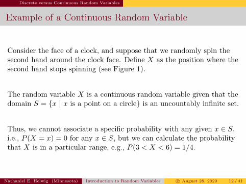
Consider the face of a clock, and suppose that we randomly spin thesecond hand around the clock face. Define X as the position where thesecond hand stops spinning (see Figure 1).

The random variable X is a continuous random variable given that thedomain S = {x | x is a point on a circle} is an uncountably infinite set.

Thus, we cannot associate a specific probability with any given x ∈ S,i.e., P (X = x) = 0 for any x ∈ S, but we can calculate the probabilitythat X is in a particular range, e.g., P (3 < X < 6) = 1/4.



Example of a Continuous Random Variable (continued)

1

2

3

4

56

7

8

9

10

1112

1

2

3

4

56

7

8

9

10

1112

1

2

3

4

56

7

8

9

10

1112

Figure 1: Clock face with three random positions of the second hand.


Probability Mass and Density Functions

Table of Contents











Probability Mass Function

The probability mass function (PMF) of a discrete random variable Xis the function f(·) that associates a probability with each x ∈ S.

• f(x) = P (X = x) ≥ 0 for any x ∈ S• ∑

x∈S f(x) = 1

0 1 2 3 4 5

0.05

0.15

0.25

n = 5

x

P(X

= x

)

0 2 4 6 8 100.

000.

100.

20

n = 10

x

P(X

= x

)

Figure 2: PMF for coin flipping example with n = 5 and n = 10.



Probability Density Function

The probability density function (PDF) of a continuous randomvariable X is the function f(·) that associates a probability with eachrange of realizations of X.

• f(x) ≥ 0 for any x ∈ S•∫ ba f(x)dx = P (a < X < b) ≥ 0 for any a, b ∈ S satisfying a < b

•∫x∈S f(x)dx = 1

Suppose that we randomly spin the second hand around a clock face nindependent times. Define Zi as the position where the second handstops spinning on the i-th replication, and define X = 1

n

∑ni=1 Zi as the

average of the n spin results. Note that the realizations of X are anyvalues x ∈ [0, 12], which is the same domain as Zi for i = 1, . . . , n.



Probability Density Function (continued)

With n = 1 spin, the PDF is simply a flat line between 0 and 12.With n = 5 spins, the PDF has a bell shape, where values around themidpoint of x = 6 have the largest density.

0 2 4 6 8 10 12

0.04

0.06

0.08

n = 1

x

f(x

)

0 2 4 6 8 10 12

0.00

0.10

0.20

n = 5

x

f(x

)

Figure 3: PDF for clock spinning example with n = 1 and n = 5.


Cumulative Distribution Function

Table of Contents











Definition of Cumulative Distribution Function

The cumulative distribution function (CDF) of a random variable X isthe function F (·) that returns the probability P (X ≤ x) for any x ∈ S.

Note that the CDF is the same as the probability distribution that wasdefined in the “Introduction to Probability” notes, such that the CDFis a function from S to [0, 1], i.e., F : S → [0, 1].

Probabilities can be written in terms of the CDF, such as

P (a < X ≤ b) = F (b)− F (a)

given that the CDF is related to the PMF (or PDF), such as

• f(x) = F (x)− lima→x− F (a) for discrete random variables

• f(x) = dF (x)dx for continuous random variables



Examples of Cumulative Distribution Functions

CDF can be defined for both discrete and continuous random variables:

• F (x) =∑

z∈S,z≤x f(z) for discrete random variables

• F (x) =∫ x−∞ f(z)dz for continuous random variables

0 1 2 3 4 5

0.0

0.4

0.8

coin flipping (n = 5)

x

F(x

)

0 2 4 6 8 10 120.

00.

40.

8

clock spinning (n = 5)

x

F(x

)

Figure 4: CDF for the coin and clock examples with n = 5.


Quantile Function

Table of Contents










Quantile Function

Definition of Quantile Function

The quantile function of a random variable X is the function Q(·) thatreturns the realization x such that P (X ≤ x) = p for any p ∈ [0, 1].

Formally, quantile function can be defined as Q(p) = minx∈S F (x) ≥ p.Thus, for any input probability p ∈ [0, 1], the quantile function Q(p)returns the smallest x ∈ S that satisfies the inequality F (x) ≥ p.

Note that the quantile function is the inverse of the CDF, such thatQ(·) is a function from [0, 1] to S, i.e., Q : [0, 1]→ S.

• For continuous random variables, we have that Q = F−1


Quantile Function

Quartiles and Percentiles

The quartiles are most commonly used percentiles:

• First Quartile: p = 1/4 returns x that cuts off the lower 25%

• Second Quartile (Median): p = 1/2 returns x that cuts thedistribution in half

• Third Quartile: p = 3/4 returns x that cuts off the upper 25%

The 100pth percentile of a distribution is the quantile x such that100p% of the distribution is below x for any p ∈ (0, 1).

• 10th percentile is the quantile corresponding to p = 1/10





Quantile Function

Visualization of Quartiles

0 2 4 6 8 10 12

0.04

0.06

0.08

n = 1

x

f(x

)

0 2 4 6 8 10 12

0.00

0.10

0.20

n = 5

xf(

x)

Figure 5: PDF and quartiles for clock spinning example with n = 1 and n = 5.


Expected Value and Expectation Operator

Table of Contents











What to Expect of a Random Variable

Here we will define a way to measure the “center” of a distribution,which is useful for understanding what to expect of a random variable.

The expected value of a random variable X is a weighted average ofthe realizations x ∈ S with the weights defined by the PMF or PDF.

The expected value of X is defined as µ = E(X) where E(·) is theexpectation operator, which is defined as

• E(X) =∑

x∈S xf(x) for discrete random variables

• E(X) =∫x∈S xf(x)dx for continuous random variables



Insight into the Expectation Operator

To understand the expectation operator E(·), suppose that we havesampled n independent realizations of some random variable X.

Let x1, . . . , xn denote the n independent realizations of X, and definethe arithmetic mean as x̄n = 1

n

∑ni=1 xi.

As the sample size n gets infinitely large, the arithmetic meanconverges to the expected value µ, i.e.,

µ = E(X) = limn→∞

x̄n

which is due to the weak law of large numbers (which is also known asBernoulli’s theorem).



Rules of Expectation Operators

Assume X is a random variable, and the other terms are constants.

1. E(a) = a

2. E(a+ bX) = E(a) + bE(X) = a+ bµ

3. E(X1 + · · ·+Xp) = E(X1) + · · ·+ E(Xp)

4. E(b1X1 + · · ·+ bpXp) = b1E(X1) + · · ·+ bpE(Xp)

5. E(∏p

j=1 bjXj

)=(∏p

j=1 bj

)E(∏p

j=1Xj

)6. E

(∏pj=1 bjXj

)=∏pj=1 bjE(Xj) if X1, . . . , Xp are independent

Rules 3-5 are true regardless of whether X1, . . . , Xp are independent.



Expectation Operator Example 1

For the coin flipping example, X =∑n

i=1 Zi where Zi is the i-th flip.

Applying rule 3, we have that E(X) =∑n

i=1E(Zi).

Since the coin is assumed to be fair, the expected value of Zi is

E(Zi) =

1∑x=0

xf(x) = 0

(1

2

)+ 1

(1

2

)=

1

2

for any given i ∈ {1, . . . , n}.

The expected value of X can be written as E(X) =∑n

i=1(1/2) = n/2



Expectation Operator Example 2

For the clock spinning example, note that X =∑n

i=1 aiZi where Zi isthe i-th clock spin and ai = 1/n for all i = 1, . . . , n.

Applying rule 4, we have that E(X) = 1n

∑ni=1E(Zi) = 1

n

∑ni=1E(Z).

Note that f(z) = 112 for z ∈ [0, 12], which implies that

E(Z) =1

12

∫ 12

0zdz =

1

12

[1

2z2]z=12

z=0

=1

24(144− 0) = 6

which implies that E(X) = 1n

∑ni=1 6 = 1

n(6n) = 6.


Variance and Standard Deviation

Table of Contents











Measuring the Spread of a Distribution

In this section, we will see that the expectation operator can also beused to help use quantify the “spread” of a distribution.

The variance of a random variable X is a weighted average of thesquared deviation between a random variable’s realizations and itsexpectation with the weights defined according to the PMF or PDF,i.e., σ2 = E[(X − µ)2] = E(X2)− µ2.• E[(X − µ)2] =

∑x∈S(x− µ)2f(x) for discrete random variables

• E[(X −µ)2] =∫x∈S(x−µ)2f(x)dx for continuous random variables

The variance of X is the expected value of the squared X minus thesquare of the expected value of X.



Insight into the Variance Operator

To gain some insight into the variance, suppose that we have sampledn independent realizations of some random variable X.

Let x1, . . . , xn denote the n independent realizations of X, and definethe arithmetic mean of the squared deviations from the average value,i.e., s̃2n = 1

n

∑ni=1(xi − x̄n)2 where x̄n = 1

n

∑ni=1 xi.

As the sample size n gets infinitely large, the arithmetic mean of thesquared deviations converges to the variance σ2, i.e.,

σ2 = E[(X − µ)2] = limn→∞

s̃2n

which is due to the weak law of large numbers (which is also known asBernoulli’s theorem).



Rules of Variance Operators

Assume X is a random variable, and the other terms are constants.

1. Var(a) = 0

2. Var(a+ bX) = Var(a) + b2Var(X) = b2σ2

3. Var(∑p

j=1Xj

)=∑p

j=1 Var(Xj) if X1, . . . , Xp are independent

4. Var(∑p

j=1 bjXj

)=∑p

j=1 b2jVar(Xj) if X1, . . . , Xp are independent

5. Var(∑p

j=1 bjXj

)=∑p

j=1 b2jVar(Xj) + 2

∑pj=2

∑j−1k=1 bjbkCov(Xj , Xk),

where Cov(Xj , Xk) = E[(Xj − µj)(Xk − µk)] is the covariance

Rules 3 and 4 are only true if X1, . . . , Xp are independent.



Variance Operator Example 1

For the coin flipping example, remember that X =∑n

i=1 Zi where Zi isthe i-th coin flip.

Applying rule 3 (which is valid because the Zi are independent), wehave that the variance of X can be written as Var(X) =

∑ni=1 Var(Zi).

Since the coin is assumed to be fair

Var(Zi) =

1∑x=0

(x− 1/2)2f(x) =

(1

4

)(1

2

)+

(1

4

)(1

2

)=

(1

4

)for any given i ∈ {1, . . . , n}, which uses the fact that E(Zi) = 1/2.

Thus, the variance of X can be written as Var(X) =∑n

i=1(1/4) = n/4.Nathaniel E. Helwig (Minnesota) Introduction to Random Variables c© August 28, 2020 35 / 41


Variance Operator Example 2

For the clock spinning example, remember that X =∑n

i=1 aiZi whereZi is the i-th clock spin and ai = 1/n for all i = 1, . . . , n.

Applying rule 4, we have that Var(X) = 1n2

∑ni=1 Var(Zi). And note

that Var(Zi) = Var(Z) = E(Z2)− E(Z)2 for all i = 1, . . . , n becausethe n spins are independent and identically distributed (iid).

Remembering that f(z) = 112 and E(Z) = 6, we just need to calculate

E(Z2) =1

12

∫ 12

0z2dz =

1

12

[1

3z3]z=12

z=0

=1

36(1728− 0) = 48

which implies that Var(Z) = 48− 36 = 12.

Thus, the variance of X is Var(X) = 1n2

∑ni=1 12 = 12/n.



Standard Deviation and Standardized Variables

The standard deviation of a random variable X is the square root ofthe variance of X, i.e., σ =

√E[(X − µ)2].

If X is a random variable with mean µ and variance σ2, then

Z =X − µσ

has mean E(Z) = 0 and variance Var(Z) = E(Z2) = 1. Proof:

• Note that Z = a+ bX where a = −µσ and b = 1

σ• Apply Expectation Rule 2: E(Z) = a+ bE(X) = −µ

σ + µσ = 0

• Apply Variance Rule 2: Var(Z) = b2Var(X) = σ2

σ2 = 1

A standardized variable has mean E(Z) = 0 and variance E(Z2) = 1.Such a variable is typically denoted by Z (instead of X) and may bereferred to as “z-score”.


Moments of a Distribution

Table of Contents











Raw, Central, and Standardized Moments

The k-th moment of a random variable X is the expected value of Xk,i.e., µ′k = E(Xk).

The k-th central moment of a random variable X is the expected valueof (X − µ)k, i.e., µk = E[(X − µ)k], where µ = E(X) is the expectedvalue of X.

The k-th standardized moment of a random variable X is the expectedvalue of (X − µ)k/σk, i.e., µ̃k = E[(X − µ)k]/σk, whereσ =

√E[(X − µ)2] is the standard deviation of X.

Note: The mean µ is the first moment and the variance σ2 is thesecond central moment.



Insight into the Moments of Distribution

Letting x1, . . . , xn denote the n independent realizations of X, we have

µ′k = limn→∞

1

n

n∑i=1

xki

µk = limn→∞

1

n

n∑i=1

(xi − x̄n)k

µ̃k = limn→∞

1

n

n∑i=1

(xi − x̄ns̃n

)k

where x̄n = 1n

∑ni=1 xi and s̃n =

√1n

∑ni=1(xi − x̄n)2.

Note that these are all results of the law of large numbers, which statesthat averages of iid data converge to expectations.



Skewness and Kurtosis

µ̃3 = E[(X − µ)3]/σ3 is skewness, which measures (lack of) symmetry.• Negative (or left-skewed) = heavy left tail• Positive (or right-skewed) = heavy right tail

µ̃4 = E[(X − µ)4]/σ4 is kurtosis, which measures peakedness.• Above 3 is leptokurtic (more peaked than normal)• Below 3 is platykurtic (less peaked than normal)

−4 −2 0 2 4

0.0

0.1

0.2

0.3

0.4

0.5

Left Skewed

x

f(x

)

−4 −2 0 2 4

0.0

0.1

0.2

0.3

0.4

0.5

Right Skewed

x

f(x

)

−4 −2 0 2 4

0.0

0.1

0.2

0.3

0.4

0.5

Leptokurtic

x

f(x

)

−4 −2 0 2 4

0.0

0.1

0.2

0.3

0.4

0.5

Platykurtic

x

f(x

)

Figure 6: Distributions with different values of skewness and kurtosis.


introduction to random variables - university of minnesota

Documents