random variables and probability …random variables and probability distributions 1. discrete...
TRANSCRIPT
RANDOM VARIABLES AND PROBABILITY DISTRIBUTIONS
1. DISCRETE RANDOM VARIABLES
1.1. Definition of a Discrete Random Variable. A random variable X is said to be discrete if it canassume only a finite or countable infinite number of distinct values. A discrete random variablecan be defined on both a countable or uncountable sample space.
1.2. Probability for a discrete random variable. The probability that X takes on the value x, P(X=x),is defined as the sum of the probabilities of all sample points in Ω that are assigned the value x. Wemay denote P(X=x) by p(x) or pX (x). The expression pX (x) is a function that assigns probabilitiesto each possible value x; thus it is often called the probability function for the random variable X.
1.3. Probability distribution for a discrete random variable. The probability distribution for adiscrete random variable X can be represented by a formula, a table, or a graph, which providespX (x) = P(X=x) for all x. The probability distribution for a discrete random variable assigns nonzeroprobabilities to only a countable number of distinct x values. Any value x not explicitly assigned apositive probability is understood to be such that P(X=x) = 0.
The function pX (x)= P(X=x) for each x within the range of X is called the probability distributionof X. It is often called the probability mass function for the discrete random variable X.
1.4. Properties of the probability distribution for a discrete random variable. A function canserve as the probability distribution for a discrete random variable X if and only if it s values,pX (x), satisfy the conditions:
a: pX (x) ≥ 0 for each value within its domainb:
∑
x pX(x) = 1 , where the summation extends over all the values within its domain
1.5. Examples of probability mass functions.
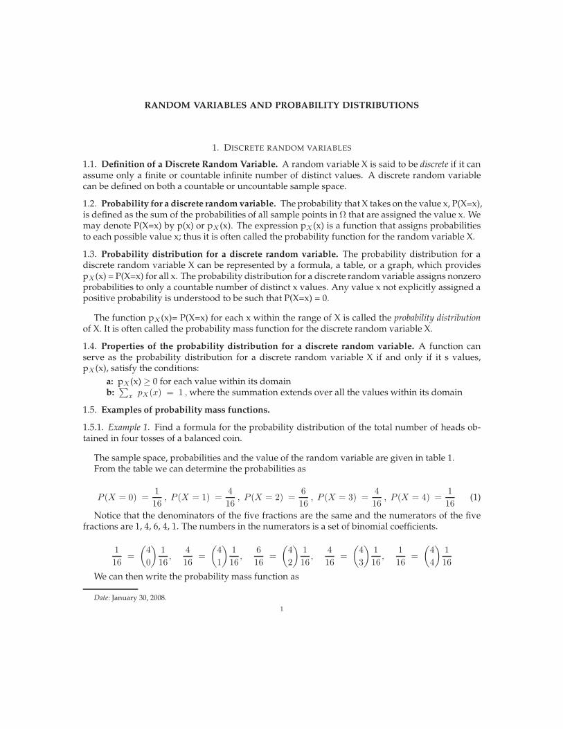
1.5.1. Example 1. Find a formula for the probability distribution of the total number of heads ob-tained in four tosses of a balanced coin.
The sample space, probabilities and the value of the random variable are given in table 1.From the table we can determine the probabilities as
P (X = 0) =1
16, P (X = 1) =
4
16, P (X = 2) =
6
16, P (X = 3) =
4
16, P (X = 4) =
1
16(1)
Notice that the denominators of the five fractions are the same and the numerators of the fivefractions are 1, 4, 6, 4, 1. The numbers in the numerators is a set of binomial coefficients.
1
16=
(
4
0
)
1
16,
4
16=
(
4
1
)
1
16,
6
16=
(
4
2
)
1
16,
4
16=
(
4
3
)
1
16,
1
16=
(
4
4
)
1
16
We can then write the probability mass function as
Date: January 30, 2008.
1
2 RANDOM VARIABLES AND PROBABILITY DISTRIBUTIONS
TABLE 1. Probability of a Function of the Number of Heads from Tossing a CoinFour Times.
Table R.1Tossing a Coin Four Times
Element of sample space Probability Value of random variable X (x)HHHH 1/16 4HHHT 1/16 3HHTH 1/16 3HTHH 1/16 3THHH 1/16 3HHTT 1/16 2HTHT 1/16 2HTTH 1/16 2THHT 1/16 2THTH 1/16 2TTHH 1/16 2HTTT 1/16 1THTT 1/16 1TTHT 1/16 1TTTH 1/16 1TTTT 1/16 0
pX(x) =
(
4x
)
16for x = 0 , 1 , 2 , 3 , 4 (2)
Note that all the probabilities are positive and that they sum to one.
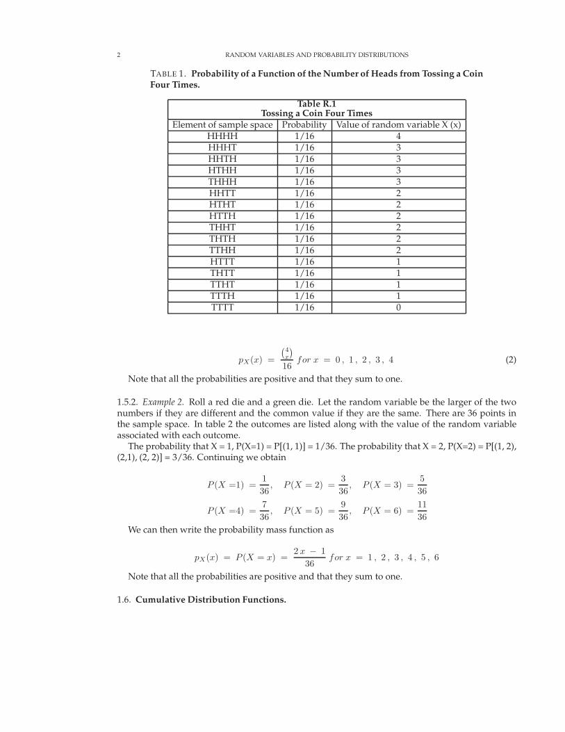
1.5.2. Example 2. Roll a red die and a green die. Let the random variable be the larger of the twonumbers if they are different and the common value if they are the same. There are 36 points inthe sample space. In table 2 the outcomes are listed along with the value of the random variableassociated with each outcome.
The probability that X = 1, P(X=1) = P[(1, 1)] = 1/36. The probability that X = 2, P(X=2) = P[(1, 2),(2,1), (2, 2)] = 3/36. Continuing we obtain
P (X =1) =1
36, P (X = 2) =
3
36, P (X = 3) =
5
36
P (X =4) =7
36, P (X = 5) =
9
36, P (X = 6) =
11
36
We can then write the probability mass function as
pX(x) = P (X = x) =2 x − 1
36for x = 1 , 2 , 3 , 4 , 5 , 6
Note that all the probabilities are positive and that they sum to one.
1.6. Cumulative Distribution Functions.
RANDOM VARIABLES AND PROBABILITY DISTRIBUTIONS 3
TABLE 2. Possible Outcomes of Rolling a Red Die and a Green Die – First Numberin Pair is Number on Red Die
Green (A) 1 2 3 4 5 6Red (D)
11 11
1 22
1 33
1 44
1 55
1 66
22 12
2 22
2 33
2 44
2 55
2 66
33 13
3 23
3 33
3 44
3 55
3 66
44 14
4 24
4 34
4 44
4 55
4 66
55 15
5 25
5 35
5 45
5 55
5 66
66 16
6 26
6 36
6 46
6 56
6 66
1.6.1. Definition of a Cumulative Distribution Function. If X is a discrete random variable, the functiongiven by
FX(x) = P (x ≤ X) =∑
t≤x
p(t) for − ∞ ≤ x ≤ ∞ (3)
where p(t) is the value of the probability distribution of X at t, is called the cumulative distributionfunction of X. The function FX (x) is also called the distribution function of X.
1.6.2. Properties of a Cumulative Distribution Function. The values FX (X) of the distribution functionof a discrete random variable X satisfy the conditions
1: F(-∞) = 0 and F(∞) =1;2: If a < b, then F(a) ≤ F(b) for any real numbers a and b
1.6.3. First example of a cumulative distribution function. Consider tossing a coin four times. Thepossible outcomes are contained in table 1 and the values of p(·) in equation 2. From this we candetermine the cumulative distribution function as follows.
F (0) = p(0) =1
16
F (1) = p(0) + p(1) =1
16+
4
16=
5
16
F (2) = p(0) + p(1) + p(2) =1
16+
4
16+
6
16=
11
16
F (3) = p(0) + p(1) + p(2) + p(3) =1
16+
4
16+
6
16+
4
6=
15
16
F (4) = p(0) + p(1) + p(2) + p(3) + p(4) =1
16+
4
16+
6
16+
4
6+
1
16=
16
16
We can write this in an alternative fashion as
4 RANDOM VARIABLES AND PROBABILITY DISTRIBUTIONS
FX(x) =
0 for x < 0116 for 0 ≤ x < 1516 for 1 ≤ x < 21116 for 2 ≤ x < 31516 for 3 ≤ x < 4
1 for x ≥ 4
1.6.4. Second example of a cumulative distribution function. Consider a group of N individuals, M ofwhom are female. Then N-M are male. Now pick n individuals from this population without
replacement. Let x be the number of females chosen. There are(
Mx
)
ways of choosing x females
from the M in the population and(
N −Mn−x
)
ways of choosing n-x of the N - M males. Therefore,
there are(
Mx
)
×(
N − Mn−x
)
ways of choosing x females and n-x males. Because there are(
Nn
)
ways ofchoosing n of the N elements in the set, and because we will assume that they all are equally likelythe probability of x females in a sample of size n is given by
pX(x) = P (X = x) =
(
Mx
) (
N −Mn−x
)
(
Nn
) for x = 0 , 1 , 2 , 3 , · · · , n
and x ≤ M, and n − x ≤ N − M.
(4)
For this discrete distribution we compute the cumulative density by adding up the appropriateterms of the probability mass function.
F (0) = p(0)
F (1) = p(0) + p(1)
F (2) = p(0) + p(1) + p(2)
F (3) = p(0) + p(1) + p(2) + px(3)
...
F (n) = p(0) + p(1) + p(2) + p(3) + · · · + p(n)
(5)
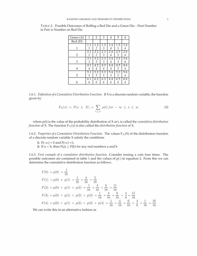
Consider a population with four individuals, three of whom are female, denoted respectivelyby A, B, C, D where A is a male and the others are females. Then consider drawing two from this
population. Based on equation 4 there should be(
42
)
= 6 elements in the sample space. The samplespace is given by
TABLE 3. Drawing Two Individuals from a Population of Four where OrderDoes Not Matter (no replacement)
Element of sample space Probability Value of random variable XAB 1/6 1AC 1/6 1AD 1/6 1BC 1/6 2BD 1/6 2CD 1/6 2
RANDOM VARIABLES AND PROBABILITY DISTRIBUTIONS 5
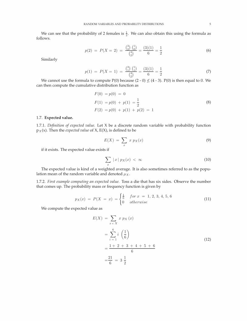
We can see that the probability of 2 females is 12 . We can also obtain this using the formula as
follows.
p(2) = P (X = 2) =
(
32
) (
10
)
(
42
) =(3)(1)
6=
1
2(6)
Similarly
p(1) = P (X = 1) =
(
31
) (
11
)
(
42
) =(3)(1)
6=
1
2(7)
We cannot use the formula to compute P(0) because (2 - 0) 6≤ (4 - 3). P(0) is then equal to 0. Wecan then compute the cumulative distribution function as
F (0) = p(0) = 0
F (1) = p(0) + p(1) =1
2F (2) = p(0) + p(1) + p(2) = 1
(8)
1.7. Expected value.
1.7.1. Definition of expected value. Let X be a discrete random variable with probability functionpX (x). Then the expected value of X, E(X), is defined to be
E(X) =∑
x
x pX(x) (9)
if it exists. The expected value exists if
∑
x
|x | pX(x) < ∞ (10)
The expected value is kind of a weighted average. It is also sometimes referred to as the popu-lation mean of the random variable and denoted µX .
1.7.2. First example computing an expected value. Toss a die that has six sides. Observe the numberthat comes up. The probability mass or frequency function is given by
pX(x) = P (X = x) =
16 for x = 1, 2, 3, 4, 5, 6
0 otherwise(11)
We compute the expected value as
E(X) =∑
x ǫ X
x pX (x)
=
6∑
i = 1
i
(
1
6
)
=1 + 2 + 3 + 4 + 5 + 6
6
=21
6= 3
1
2
(12)
6 RANDOM VARIABLES AND PROBABILITY DISTRIBUTIONS
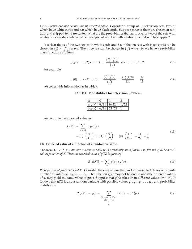
1.7.3. Second example computing an expected value. Consider a group of 12 television sets, two ofwhich have white cords and ten which have black cords. Suppose three of them are chosen at ran-dom and shipped to a care center. What are the probabilities that zero, one, or two of the sets withwhite cords are shipped? What is the expected number with white cords that will be shipped?
It is clear that x of the two sets with white cords and 3-x of the ten sets with black cords can bechosen in
(
2x
)
×(
103−x
)
ways. The three sets can be chosen in(
123
)
ways. So we have a probability
mass function as follows.
pX(x) = P (X = x) =
(
2x
) (
103−x
)
(
123
) for x = 0 , 1 , 2 (13)
For example
p(0) = P (X = 0) =
(
20
) (
103−0
)
(
123
) =(1) (120)
220=
6
11(14)
We collect this information as in table 4.
TABLE 4. Probabilities for Television Problem
x 0 1 2pX (x) 6/11 9/22 1/22FX (x) 6/11 21/22 1
We compute the expected value as
E(X) =∑
x ǫ X
x pX (x)
= (0)
(
6
11
)
+ (1)
(
9
22
)
+ (2)
(
1
22
)
=11
22=
1
2
(15)
1.8. Expected value of a function of a random variable.
Theorem 1. Let X be a discrete random variable with probability mass function pX (x) and g(X) be a real-valued function of X. Then the expected value of g(X) is given by
E[g(X)] =∑
x
g(x) pX(x) . (16)
Proof for case of finite values of X. Consider the case where the random variable X takes on a finitenumber of values x1, x2, x3, · · ·xn. The function g(x) may not be one-to-one (the different valuesof xi may yield the same value of g(xi). Suppose that g(X) takes on m different values (m ≤ n). Itfollows that g(X) is also a random variable with possible values g1, g2, g3, . . . gm and probabilitydistribution
P [g(X) = gi] =∑
∀ xjsuch that
g(xj) = gi
j
p(xj) = p∗ (gi) (17)
RANDOM VARIABLES AND PROBABILITY DISTRIBUTIONS 7
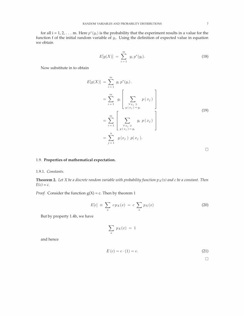
for all i = 1, 2, . . . m. Here p∗(gi) is the probability that the experiment results in a value for thefunction f of the initial random variable of gi. Using the definition of expected value in equationwe obtain
E[g(X)] =
m∑
i =1
gi p∗(gi). (18)
Now substitute in to obtain
E[g(X)] =m
∑
i =1
gi p∗(gi) .
=
m∑
i =1
gi
∑
∀ xj ∋g ( xj ) = gi
p (xj )
=
m∑
i =1
∑
∀ xj ∋g ( xj )= gi
gi p (xj )
=n
∑
j =1
g (xj ) p(xj ).
(19)
1.9. Properties of mathematical expectation.
1.9.1. Constants.
Theorem 2. Let X be a discrete random variable with probability function pX(x) and c be a constant. ThenE(c) = c.
Proof. Consider the function g(X) = c. Then by theorem 1
E[c] ≡∑
x
c pX(x) = c∑
x
pX(x) (20)
But by property 1.4b, we have
∑
x
pX(x) = 1
and hence
E (c) = c · (1) = c. (21)
8 RANDOM VARIABLES AND PROBABILITY DISTRIBUTIONS
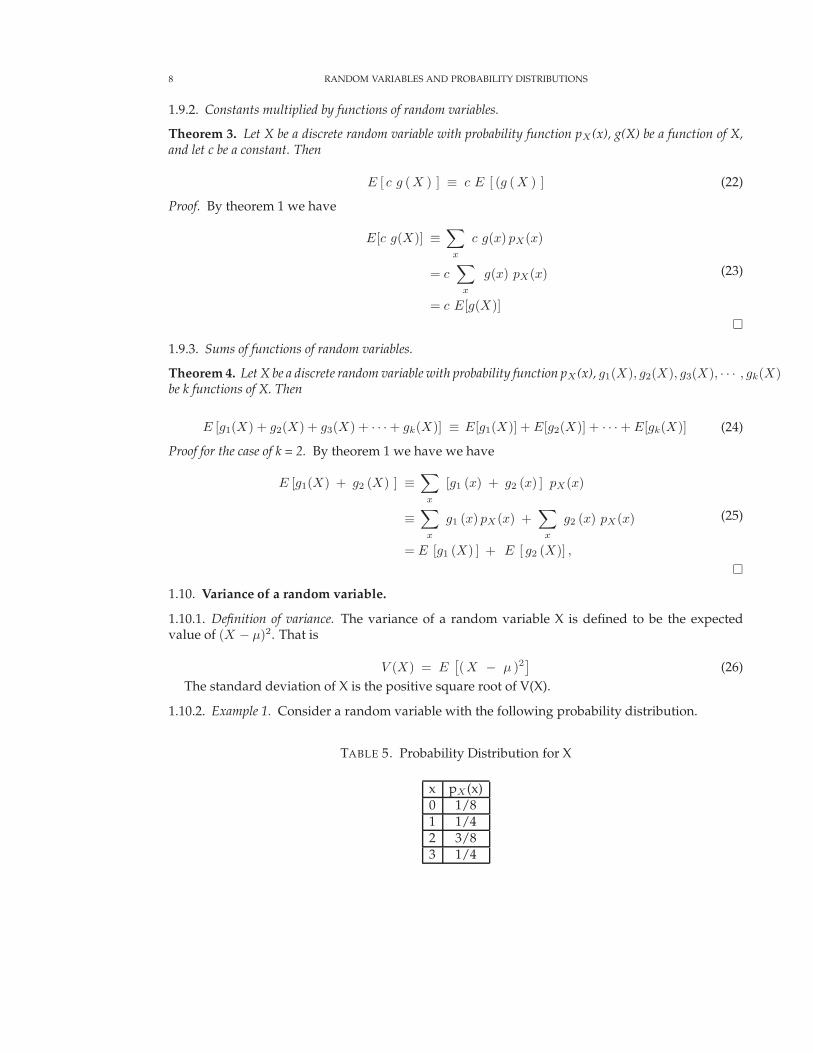
1.9.2. Constants multiplied by functions of random variables.
Theorem 3. Let X be a discrete random variable with probability function pX (x), g(X) be a function of X,and let c be a constant. Then
E [ c g (X ) ] ≡ c E [ (g (X ) ] (22)
Proof. By theorem 1 we have
E[c g(X)] ≡∑
x
c g(x) pX(x)
= c∑
x
g(x) pX(x)
= c E[g(X)]
(23)
1.9.3. Sums of functions of random variables.
Theorem 4. Let X be a discrete random variable with probability function pX (x), g1(X), g2(X), g3(X), · · · , gk(X)be k functions of X. Then
E [g1(X) + g2(X) + g3(X) + · · · + gk(X)] ≡ E[g1(X)] + E[g2(X)] + · · · + E[gk(X)] (24)
Proof for the case of k = 2. By theorem 1 we have we have
E [g1(X) + g2 (X) ] ≡∑
x
[g1 (x) + g2 (x) ] pX(x)
≡∑
x
g1 (x) pX(x) +∑
x
g2 (x) pX(x)
= E [g1 (X) ] + E [ g2 (X)] ,
(25)
1.10. Variance of a random variable.
1.10.1. Definition of variance. The variance of a random variable X is defined to be the expectedvalue of (X − µ)2. That is
V (X) = E[
(X − µ )2]
(26)
The standard deviation of X is the positive square root of V(X).
1.10.2. Example 1. Consider a random variable with the following probability distribution.
TABLE 5. Probability Distribution for X
x pX (x)0 1/81 1/42 3/83 1/4
RANDOM VARIABLES AND PROBABILITY DISTRIBUTIONS 9
We can compute the expected value as
µ = E(X) =
3∑
x =0
x pX (x)
= (0)
(
1
8
)
+ (1)
(
1
4
)
+ (2)
(
3
8
)
+ (3)
(
1
4
)
= 13
4
(27)
We compute the variance as
σ2 = E[X − µ)2] = Σ3x= 0 (x − µ)2 pX(x)
= (0 − 1.75)2(
1
8
)
+ (1 − 1.75)2(
1
4
)
+ (2 − 1.75)2(
3
8
)
+ (3 − 1.75)2(
1
4
)
= .9375
and the standard deviation as
σ2 = 0.9375
σ = +√
σ2 =√
.9375 = 0.97.
1.10.3. Alternative formula for the variance.
Theorem 5. Let X be a discrete random variable with probability function pX (x); then
V (X) ≡ σ2 = E[
(X − µ )2]
= E(
X2)
− µ2 (28)
Proof. First write out the first part of equation 28 as follows
V (X) ≡ σ2 = E[
(X − µ )2]
= E(
X2 − 2 µ X + µ2)
= E(
X2)
− E (2 µ X) + E(
µ2) (29)
where the last step follows from theorem 4. Note that µ is a constant, then apply theorems 3 and2 to the second and third terms in equation 28 to obtain
V (X) ≡ σ2 = E[
(X − µ )2]
= E(
X2)
− 2 µ E (X) + µ2 (30)
Then making the substitution that E(X) = µ, we obtain
V (X) ≡ σ2 = E(
X2)
− µ2 (31)
1.10.4. Example 2. Die toss.Toss a die that has six sides. Observe the number that comes up. The probability mass or fre-
quency function is given by
pX(x) = P (X = x) =
16 for x = 1, 2, 3, 4, 5, 6
0 otherwise. (32)
We compute the expected value as
10 RANDOM VARIABLES AND PROBABILITY DISTRIBUTIONS
E(X) =∑
x ǫ X
x pX (x)
=
6∑
i = 1
i
(
1
6
)
=1 + 2 + 3 + 4 + 5 + 6
6
=21
6= 3
1
2
(33)
We compute the variance by then computing the E(X2) as follows
E(X2) =∑
x ǫ X
x2 pX (x)
=
6∑
i = 1
i2(
1
6
)
=1 + 4 + 9 + 16 + 25 + 36
6
=91
6= 15
1
6
(34)
We can then compute the variance using the formula Var(X) = E(X 2) - E 2(X) and the fact theE(X) = 21/6 from equation 33.
V ar(X) = E (X2) − E2(X)
=91
6−
(
21
6
)2
=91
6−
(
441
36
)
=546
36− 441
36
=105
36=
35
12= 2.9166
(35)
RANDOM VARIABLES AND PROBABILITY DISTRIBUTIONS 11
2. THE ”DISTRIBUTION” OF RANDOM VARIABLES IN GENERAL
2.1. Cumulative distribution function. The cumulative distribution function (cdf) of a randomvariable X, denoted by FX (·), is defined to be the function with domain the real line and range theinterval [0,1], which satisfies FX (x) = PX [X ≤ x] = P [ ω : X(ω) ≤ x ] for every real number x.F has the following properties:
FX(−∞) = limx→−∞
FX(x) = 0, FX(+∞) = limx→+∞
FX(x) = 1, (36a)
FX(a) ≤ FX(b) for a < b, nondecreasing function of x, (36b)
lim0<h→0
FX(x + h) = FX(x), continuous from the right, (36c)
2.2. Example of a cumulative distribution function. Consider the following function
FX (x) =1
1 + e−x(37)
Check condition 36a as follows.
limx→−∞
FX(x) = limx→−∞
1
1 + e−x= lim
x→∞
1
1 + ex= 0
limx→∞
FX(x) = limx→∞
1
1 + e−x= 1
(38)
To check condition 36b differentiate the cdf as follows
dFX (x )
dx=
d(
11 + e−x
)
dx
=e−x
( 1 + e−x )2 > 0
(39)
Condition 36c is satisfied because FX(x) is a continuous function.
2.3. Discrete and continuous random variables.
2.3.1. Discrete random variable. A random variable X will be said to be discrete if the range of X iscountable, that is if it can assume only a finite or countably infinite number of values. Alternatively,a random variable is discrete if FX(x) is a step function of x.
2.3.2. Continuous random variable. A random variable X is continuous if FX(x) is a continuous func-tion of x.
2.4. Frequency (probability mass) function of a discrete random variable.
2.4.1. Definition of a frequency (discrete density) function. If X is a discrete random variable with thedistinct values, x1, x2, · · · , xn, · · · , then the function denoted by p(·) and defined by
pX(x) =
P [X = xj ] x = xj , j = 1, 2 , ... , n, ...
0 x 6= xj
(40)
is defined to be the frequency, discrete density, or probability mass function of X. We will oftenwrite fX (x) for pX (x) to denote frequency as compared to probability.
A discrete probability distribution on R k is a probability measure P such that
12 RANDOM VARIABLES AND PROBABILITY DISTRIBUTIONS
∞∑
i = 1
P (xi) = 1 (41)
for some sequence of points in Rk, i.e. the sequence of points that occur as an outcome of theexperiment. Given the definition of the frequency function in equation 40, we can also say that anynon-negative function p on Rk that vanishes except on a sequence x1, x2, · · · , xn, · · · of vectors andthat satisfies
∞∑
i =1
p(xi) = 1
defines a unique probability distribution by the relation
P (A ) =∑
xi ǫ A
p (xi ) (42)
2.4.2. Properties of discrete density functions. As defined in section 1.4, a probability mass functionmust satisfy
pX(xj) > 0, for j = 1, 2, ... (43a)
pX(x) = 0, for x 6= xj ; j = 1, 2, ..., (43b)
∑
j
pX(x)j = 1 (43c)
2.4.3. Example 1 of a discrete density function. Consider a probability model where there are twopossible outcomes to a single action (say heads and tails) and consider repeating this action severaltimes until one of the outcomes occurs. Let the random variable be the number of actions requiredto obtain a particular outcome (say heads). Let p be the probability that outcome is a head and (1-p)the probability of a tail. Then to obtain the first head on the xth toss, we need to have a tail on theprevious x-1 tosses. So the probability of the first had occurring on the xth toss is given by
pX(x) = P (X = x) =
(1 − p)x− 1 p for x = 1, 2 , ...
0 otherwise(44)
For example the probability that it takes 4 tosses to get a head is 1/16 while the probability ittakes 2 tosses is 1/4.
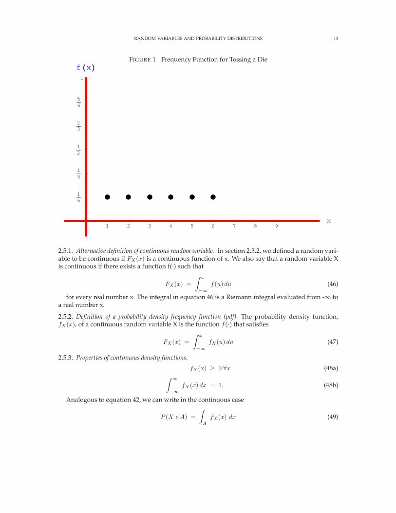
2.4.4. Example 2 of a discrete density function. Consider tossing a die. The sample space is 1, 2, 3, 4,5, 6. The elements are 1, 2, ... . The frequency function is given by
p(x) = P (X = x) =
16 for x = 1, 2, 3, 4, 5, 6
0 otherwise. (45)
The density function is represented in figure 1.
2.5. Probability density function of a continuous random variable.
RANDOM VARIABLES AND PROBABILITY DISTRIBUTIONS 13
FIGURE 1. Frequency Function for Tossing a Die
1 2 3 4 5 6 7 8 9x
1
6
1
3
1
2
2
3
5
6
1
fHxL
2.5.1. Alternative definition of continuous random variable. In section 2.3.2, we defined a random vari-able to be continuous if FX(x) is a continuous function of x. We also say that a random variable Xis continuous if there exists a function f(·) such that
FX(x) =
∫ x
−∞f(u) du (46)
for every real number x. The integral in equation 46 is a Riemann integral evaluated from -∞ toa real number x.
2.5.2. Definition of a probability density frequency function (pdf). The probability density function,fX(x), of a continuous random variable X is the function f(·) that satisfies
FX(x) =
∫ x
−∞fX(u) du (47)
2.5.3. Properties of continuous density functions.
fX(x) ≥ 0 ∀x (48a)
∫ ∞
−∞fX(x) dx = 1, (48b)
Analogous to equation 42, we can write in the continuous case
P (X ǫ A) =
∫
A
fX(x) dx (49)
14 RANDOM VARIABLES AND PROBABILITY DISTRIBUTIONS
where the integral is interpreted in the sense of Lebesgue.
Theorem 6. For a density function fX (x) defined over the set of all real numbers the following holds
P (a ≤ X ≤ b) =
∫ b
a
fX(x) dx (50)
for any real constants a and b with a ≤ b.
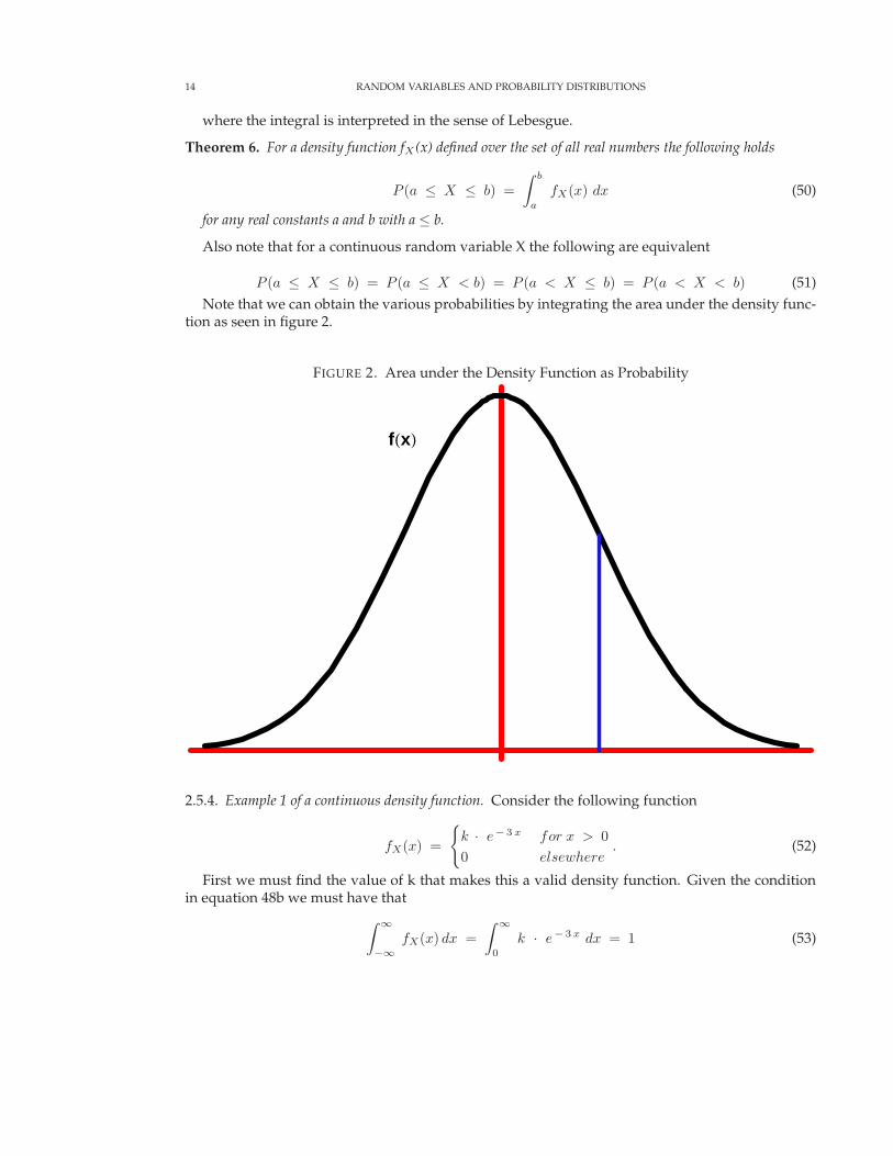
Also note that for a continuous random variable X the following are equivalent
P (a ≤ X ≤ b) = P (a ≤ X < b) = P (a < X ≤ b) = P (a < X < b) (51)
Note that we can obtain the various probabilities by integrating the area under the density func-tion as seen in figure 2.
FIGURE 2. Area under the Density Function as Probability
fHxL
2.5.4. Example 1 of a continuous density function. Consider the following function
fX(x) =
k · e− 3 x for x > 0
0 elsewhere. (52)
First we must find the value of k that makes this a valid density function. Given the conditionin equation 48b we must have that
∫ ∞
−∞fX(x) dx =
∫ ∞
0
k · e− 3 x dx = 1 (53)
RANDOM VARIABLES AND PROBABILITY DISTRIBUTIONS 15
Integrate the second term to obtain
∫ ∞
0
k · e− 3 x dx = k · limt →∞
e− 3 x
− 3|t0 =
k
3(54)
Given that this must be equal to one we obtain
k
3= 1
⇒ k = 3
(55)
The density is then given by
fX(x) =
3 · e− 3 x for x > 0
0 elsewhere. (56)
Now find the probability that (1 ≤ X ≤ 2).
P (1 ≤ X ≤ 2) =
∫ 2
1
3 · e− 3 x dx
= − e− 3 x |21= − e− 6 + e− 3
= − 0.00247875 + 0.049787
= 0.047308
(57)
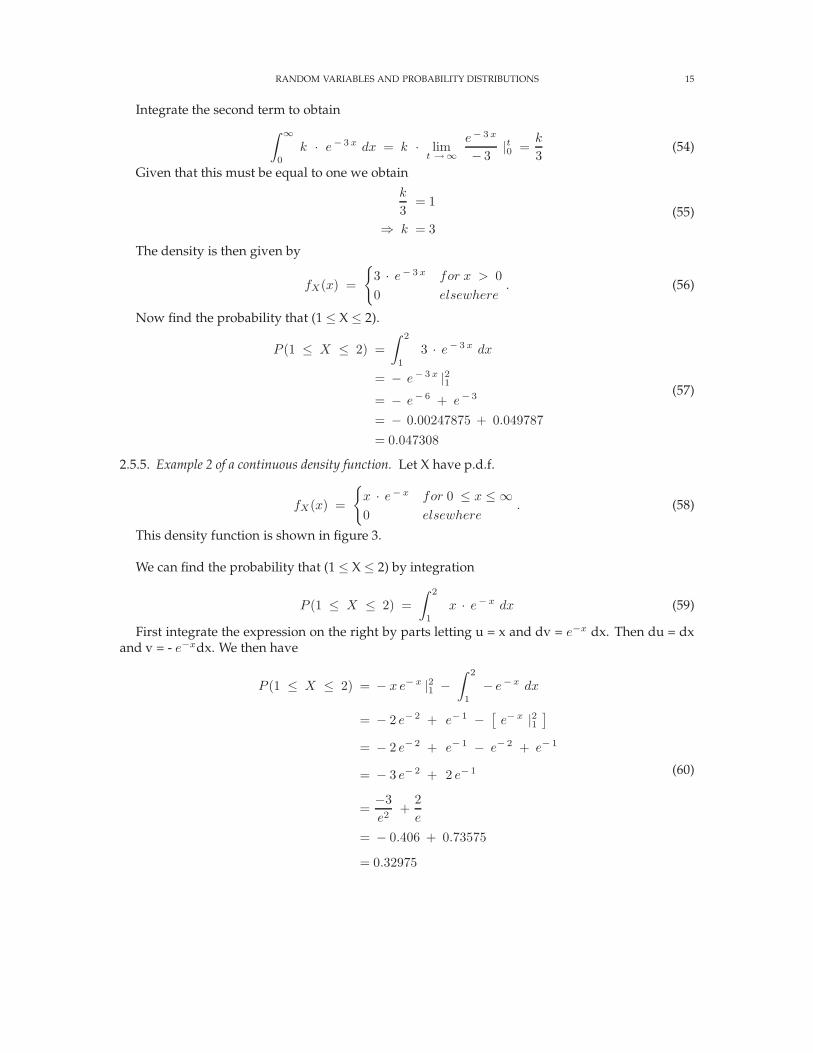
2.5.5. Example 2 of a continuous density function. Let X have p.d.f.
fX(x) =
x · e− x for 0 ≤ x ≤ ∞0 elsewhere
. (58)
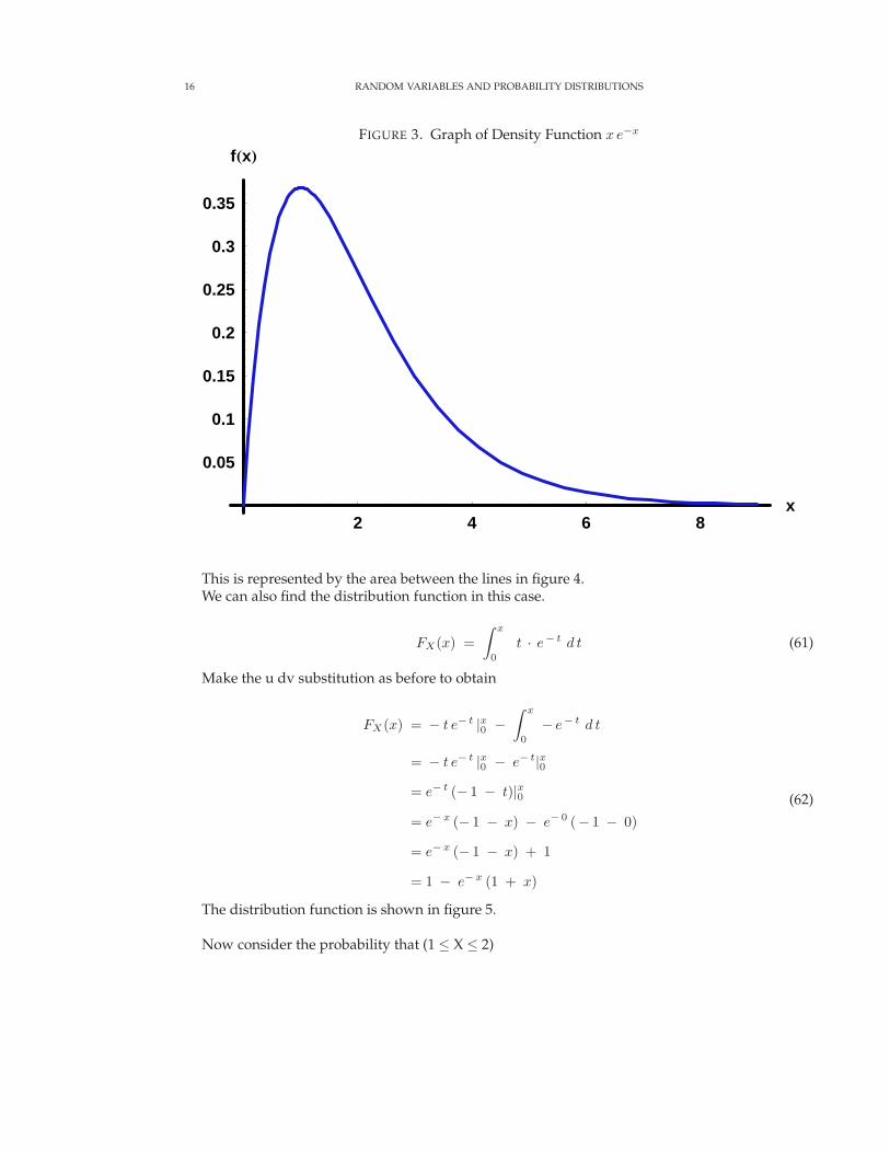
This density function is shown in figure 3.
We can find the probability that (1 ≤ X ≤ 2) by integration
P (1 ≤ X ≤ 2) =
∫ 2
1
x · e−x dx (59)
First integrate the expression on the right by parts letting u = x and dv = e−x dx. Then du = dxand v = - e−xdx. We then have
P (1 ≤ X ≤ 2) = − x e−x |21 −∫ 2
1
− e−x dx
= − 2 e− 2 + e− 1 −[
e−x |21]
= − 2 e− 2 + e− 1 − e− 2 + e− 1
= − 3 e− 2 + 2 e− 1
=−3
e2+
2
e
= − 0.406 + 0.73575
= 0.32975
(60)
16 RANDOM VARIABLES AND PROBABILITY DISTRIBUTIONS
FIGURE 3. Graph of Density Function x e−x
2 4 6 8x
0.05
0.1
0.15
0.2
0.25
0.3
0.35
fHxL
This is represented by the area between the lines in figure 4.We can also find the distribution function in this case.
FX(x) =
∫ x
0
t · e− t d t (61)
Make the u dv substitution as before to obtain
FX(x) = − t e− t |x0 −∫ x
0
− e− t d t
= − t e− t |x0 − e− t|x0= e− t (− 1 − t)|x0= e−x (− 1 − x) − e− 0 (− 1 − 0)
= e−x (− 1 − x) + 1
= 1 − e−x (1 + x)
(62)
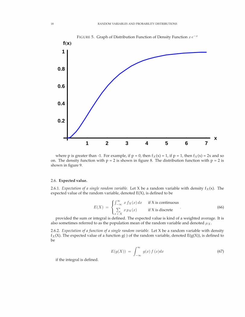
The distribution function is shown in figure 5.
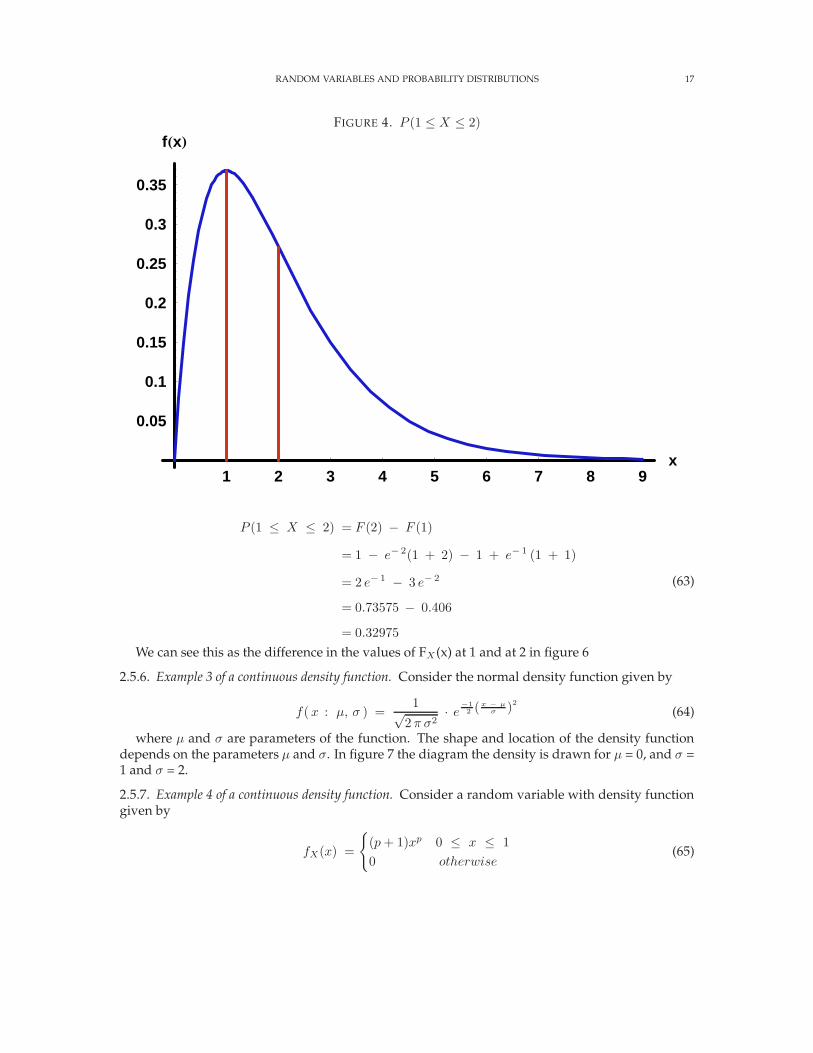
Now consider the probability that (1 ≤ X ≤ 2)
RANDOM VARIABLES AND PROBABILITY DISTRIBUTIONS 17
FIGURE 4. P (1 ≤ X ≤ 2)
1 2 3 4 5 6 7 8 9x
0.05
0.1
0.15
0.2
0.25
0.3
0.35
fHxL
P (1 ≤ X ≤ 2) = F (2) − F (1)
= 1 − e− 2(1 + 2) − 1 + e− 1 (1 + 1)
= 2 e− 1 − 3 e− 2
= 0.73575 − 0.406
= 0.32975
(63)
We can see this as the difference in the values of FX (x) at 1 and at 2 in figure 6
2.5.6. Example 3 of a continuous density function. Consider the normal density function given by
f(x : µ, σ ) =1√
2 π σ2· e
−1
2 (x − µσ )
2
(64)
where µ and σ are parameters of the function. The shape and location of the density functiondepends on the parameters µ and σ. In figure 7 the diagram the density is drawn for µ = 0, and σ =1 and σ = 2.
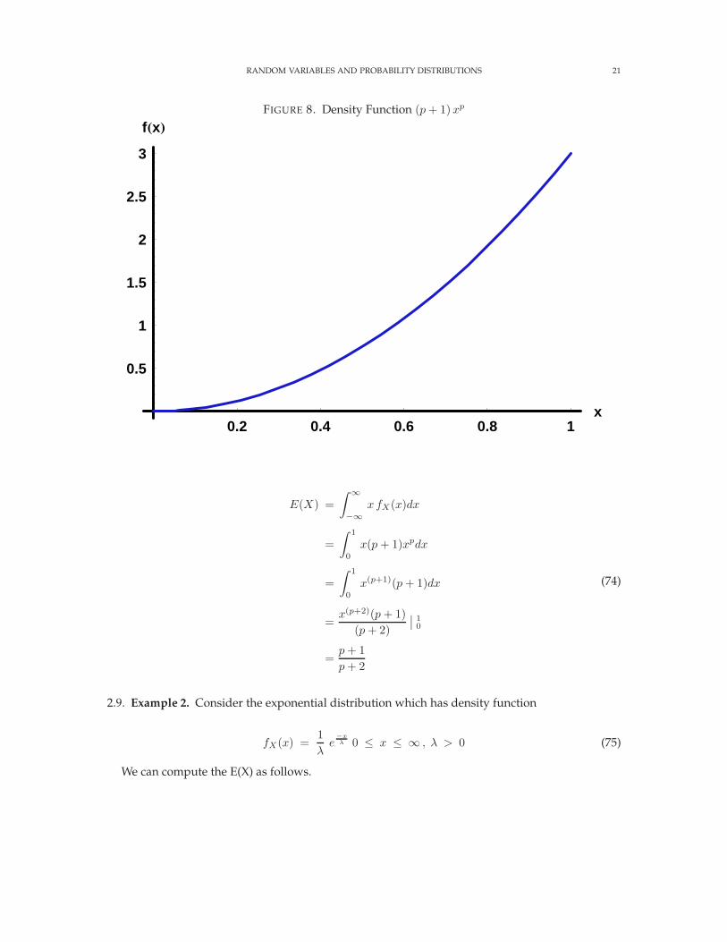
2.5.7. Example 4 of a continuous density function. Consider a random variable with density functiongiven by
fX(x) =
(p + 1)xp 0 ≤ x ≤ 1
0 otherwise(65)
18 RANDOM VARIABLES AND PROBABILITY DISTRIBUTIONS
FIGURE 5. Graph of Distribution Function of Density Function x e−x
1 2 3 4 5 6 7x
0.2
0.4
0.6
0.8
1
fHxL
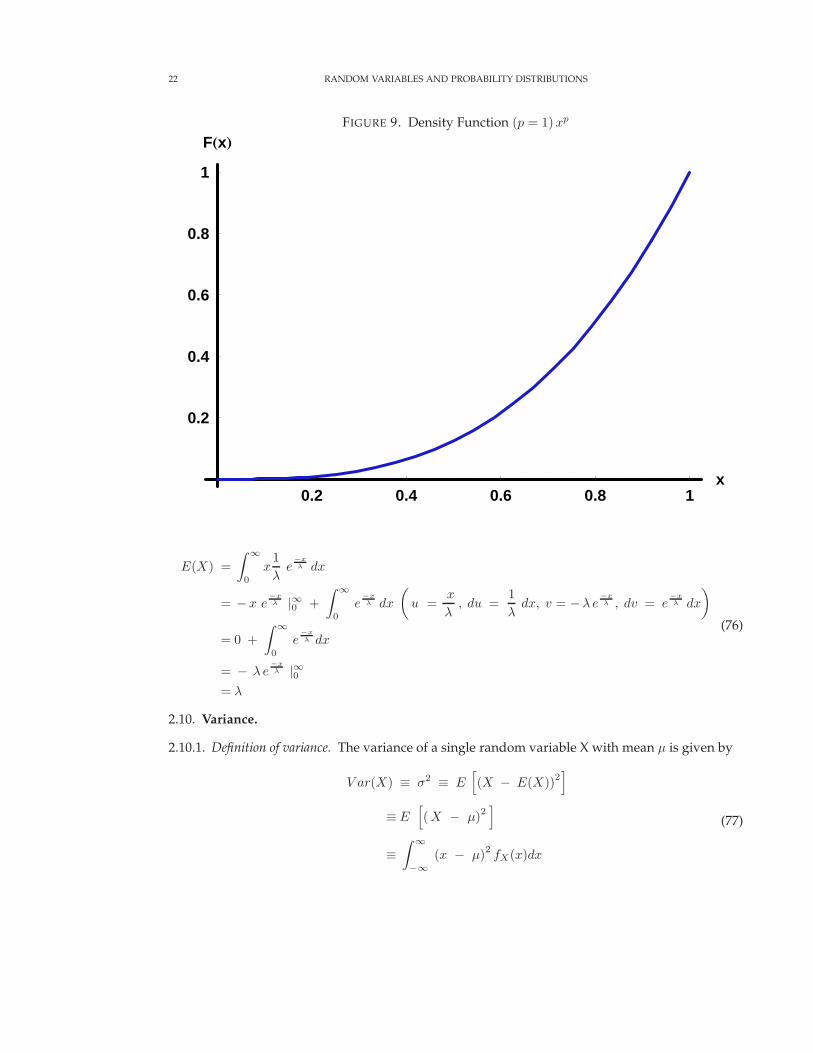
where p is greater than -1. For example, if p = 0, then fX(x) = 1, if p = 1, then fX (x) = 2x and soon. The density function with p = 2 is shown in figure 8. The distribution function with p = 2 isshown in figure 9.
2.6. Expected value.
2.6.1. Expectation of a single random variable. Let X be a random variable with density fX(x). Theexpected value of the random variable, denoted E(X), is defined to be
E(X) =
∫ ∞−∞ x fX(x) dx if X is continuous∑
x ǫ X
x pX(x) if X is discrete. (66)
provided the sum or integral is defined. The expected value is kind of a weighted average. It isalso sometimes referred to as the population mean of the random variable and denoted µX .
2.6.2. Expectation of a function of a single random variable. Let X be a random variable with densityfX(X). The expected value of a function g(·) of the random variable, denoted E(g(X)), is defined tobe
E(g(X)) =
∫ ∞
−∞g(x) f (x)dx (67)
if the integral is defined.
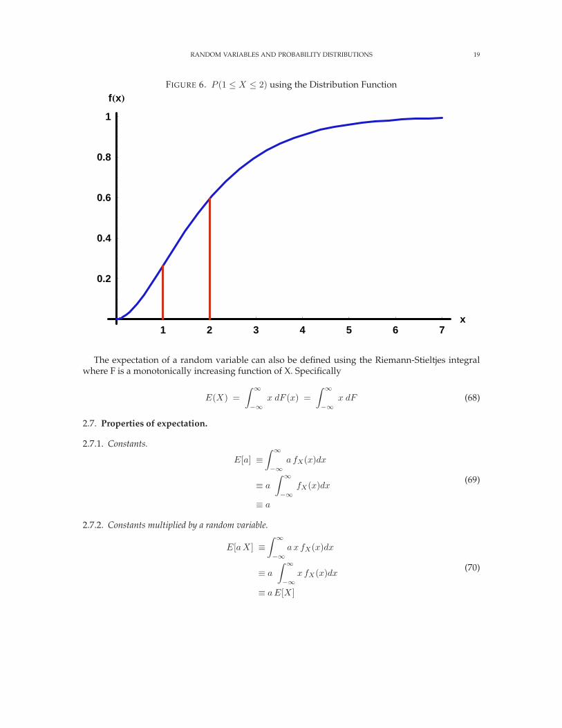
RANDOM VARIABLES AND PROBABILITY DISTRIBUTIONS 19
FIGURE 6. P (1 ≤ X ≤ 2) using the Distribution Function
1 2 3 4 5 6 7x
0.2
0.4
0.6
0.8
1
fHxL
The expectation of a random variable can also be defined using the Riemann-Stieltjes integralwhere F is a monotonically increasing function of X. Specifically
E(X) =
∫ ∞
−∞x dF (x) =
∫ ∞
−∞x dF (68)
2.7. Properties of expectation.
2.7.1. Constants.
E[a] ≡∫ ∞
−∞a fX(x)dx
≡ a
∫ ∞
−∞fX(x)dx
≡ a
(69)
2.7.2. Constants multiplied by a random variable.
E[a X ] ≡∫ ∞
−∞a x fX(x)dx
≡ a
∫ ∞
−∞x fX(x)dx
≡ a E[X ]
(70)
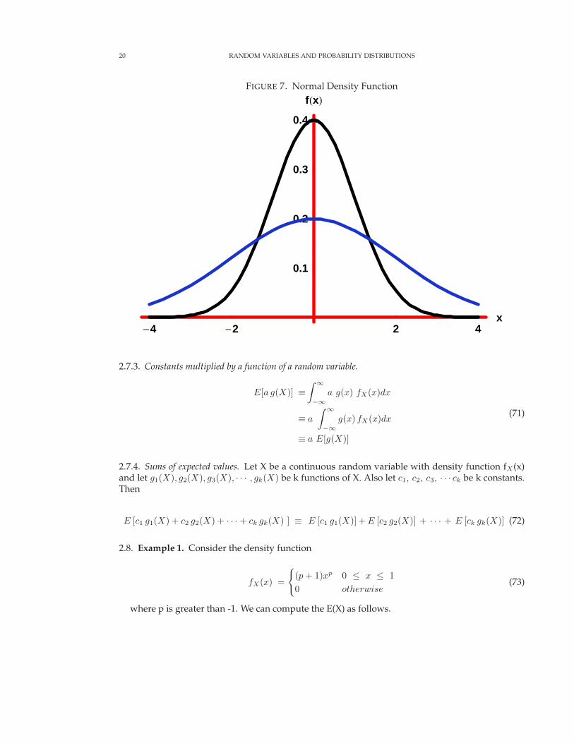
20 RANDOM VARIABLES AND PROBABILITY DISTRIBUTIONS
FIGURE 7. Normal Density Function
-4 -2 2 4x
0.1
0.2
0.3
0.4
fHxL
2.7.3. Constants multiplied by a function of a random variable.
E[a g(X)] ≡∫ ∞
−∞a g(x) fX(x)dx
≡ a
∫ ∞
−∞g(x) fX(x)dx
≡ a E[g(X)]
(71)
2.7.4. Sums of expected values. Let X be a continuous random variable with density function fX(x)and let g1(X), g2(X), g3(X), · · · , gk(X) be k functions of X. Also let c1, c2, c3, · · · ck be k constants.Then
E [c1 g1(X) + c2 g2(X) + · · · + ck gk(X) ] ≡ E [c1 g1(X)] + E [c2 g2(X)] + · · · + E [ck gk(X)] (72)
2.8. Example 1. Consider the density function
fX(x) =
(p + 1)xp 0 ≤ x ≤ 1
0 otherwise(73)
where p is greater than -1. We can compute the E(X) as follows.
RANDOM VARIABLES AND PROBABILITY DISTRIBUTIONS 21
FIGURE 8. Density Function (p + 1)xp
0.2 0.4 0.6 0.8 1x
0.5
1
1.5
2
2.5
3
fHxL
E(X) =
∫ ∞
−∞x fX(x)dx
=
∫ 1
0
x(p + 1)xpdx
=
∫ 1
0
x(p+1)(p + 1)dx
=x(p+2)(p + 1)
(p + 2)
∣
∣
10
=p + 1
p + 2
(74)
2.9. Example 2. Consider the exponential distribution which has density function
fX(x) =1
λe
−xλ 0 ≤ x ≤ ∞ , λ > 0 (75)
We can compute the E(X) as follows.
22 RANDOM VARIABLES AND PROBABILITY DISTRIBUTIONS
FIGURE 9. Density Function (p = 1)xp
0.2 0.4 0.6 0.8 1x
0.2
0.4
0.6
0.8
1
FHxL
E(X) =
∫ ∞
0
x1
λe
−xλ dx
= − x e−xλ |∞0 +
∫ ∞
0
e−xλ dx
(
u =x
λ, du =
1
λdx, v = −λ e
−xλ , dv = e
−xλ dx
)
= 0 +
∫ ∞
0
e−xλ dx
= − λ e−xλ |∞0
= λ
(76)
2.10. Variance.
2.10.1. Definition of variance. The variance of a single random variable X with mean µ is given by
V ar(X) ≡ σ2 ≡ E[
(X − E(X))2]
≡ E[
(X − µ)2]
≡∫ ∞
−∞(x − µ)2 fX(x)dx
(77)
RANDOM VARIABLES AND PROBABILITY DISTRIBUTIONS 23
We can write this in a different fashion by expanding the last term in equation 77.
V ar(X) ≡∫ ∞
−∞(x − µ)
2fX(x)dx
≡∫ ∞
−∞(x2 − 2 µ x + µ2) fX(x)dx
≡∫ ∞
−∞x2 fX(x) dx − 2 µ
∫ ∞
−∞x fX(x) dx + µ2
∫ ∞
−∞fX(x) dx
= E[
X2]
− 2 µ E [X ] + µ2
= E[
X2]
− 2 µ2 + µ2
= E[
X2]
− µ2
≡∫ ∞
−∞x2 fX(x)dx −
[∫ ∞
−∞x fX(x)dx
]2
(78)
The variance is a measure of the dispersion of the random variable about the mean.
2.10.2. Variance example 1. Consider the density function
fX(x) =
(p + 1)xp 0 ≤ x ≤ 1
0 otherwise(79)
where p is greater than -1. We can compute the Var(X) as follows.
E(X) =
∫ ∞
−∞x fX(x)dx
=
∫ 1
0
x(p + 1)xpdx
=x(p+2)(p + 1)
(p + 2)| 10
=p + 1
p + 2
E(X2 ) =
∫ 1
0
x2 (p + 1)xp dx
=x(p +3 )(p + 1)
(p + 3)| 10
=p + 1
p + 3
V ar (X ) = E (X2 ) − E2(X )
=p + 1
p + 3−
(
p + 1
p + 2
)2
=p + 1
(p + 2 )2 (p + 3 )
(80)
The values of the mean and variances for various values of p are given in table 6.
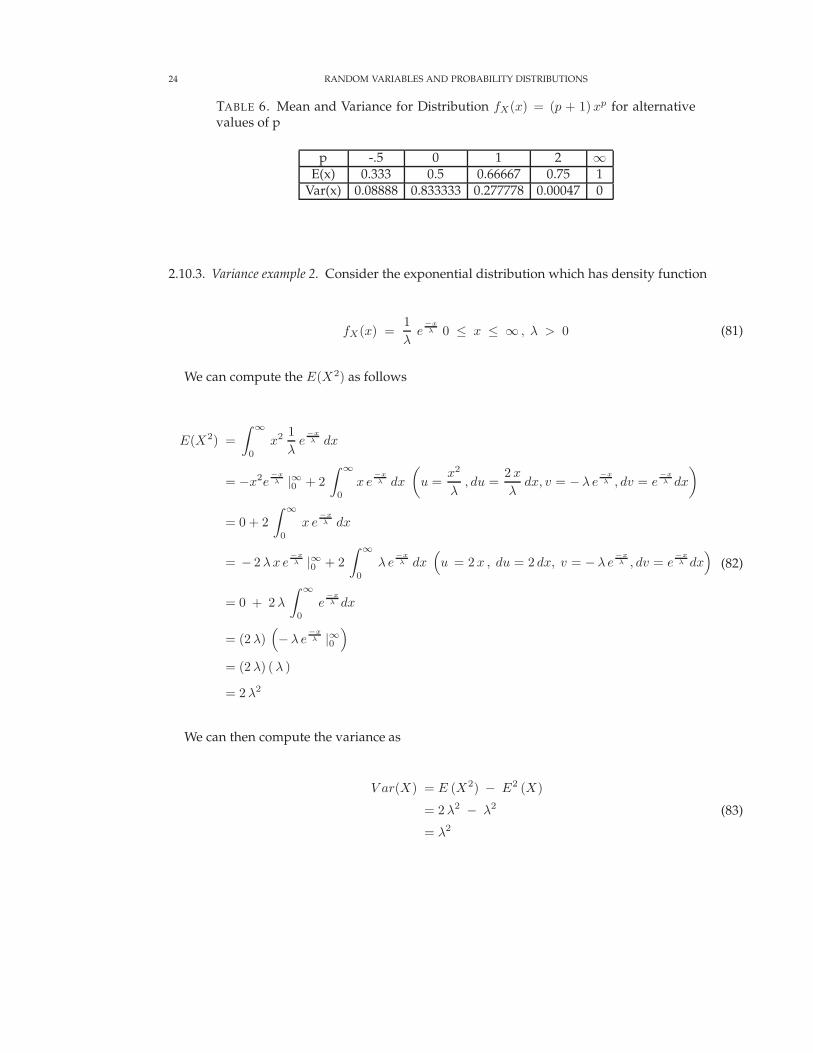
24 RANDOM VARIABLES AND PROBABILITY DISTRIBUTIONS
TABLE 6. Mean and Variance for Distribution fX(x) = (p + 1)xp for alternativevalues of p
p -.5 0 1 2 ∞E(x) 0.333 0.5 0.66667 0.75 1
Var(x) 0.08888 0.833333 0.277778 0.00047 0
2.10.3. Variance example 2. Consider the exponential distribution which has density function
fX(x) =1
λe
−xλ 0 ≤ x ≤ ∞ , λ > 0 (81)
We can compute the E(X2) as follows
E(X2) =
∫ ∞
0
x2 1
λe
−xλ dx
= −x2e−xλ |∞0 + 2
∫ ∞
0
x e−xλ dx
(
u =x2
λ, du =
2 x
λdx, v = −λ e
−xλ , dv = e
−xλ dx
)
= 0 + 2
∫ ∞
0
x e−xλ dx
= − 2 λx e−xλ |∞0 + 2
∫ ∞
0
λ e−xλ dx
(
u = 2 x , du = 2 dx, v = −λ e−xλ , dv = e
−xλ dx
)
= 0 + 2 λ
∫ ∞
0
e−xλ dx
= (2 λ)(
−λ e−xλ |∞0
)
= (2 λ) (λ )
= 2 λ2
(82)
We can then compute the variance as
V ar(X) = E (X2) − E2 (X)
= 2 λ2 − λ2
= λ2
(83)
RANDOM VARIABLES AND PROBABILITY DISTRIBUTIONS 25
3. MOMENTS AND MOMENT GENERATING FUNCTIONS
3.1. Moments.
3.1.1. Moments about the origin (raw moments). The rth moment about the origin of a random vari-able X, denoted by µ′
r, is the expected value of Xr; symbolically,
µ′r = E(Xr)
=∑
x
xrfX(x) (84)
for r = 0, 1, 2, . . . when X is discrete and
µ′r = E(Xr)
=
∫ ∞
−∞xrfX(x) dx
(85)
when X is continuous. The rth moment about the origin is only defined if E[Xr] exists. Amoment about the origin is sometimes called a raw moment. Note that µ′
1 = E(X) = µX , themean of the distribution of X, or simply the mean of X. The rth moment is sometimes written as afunction of θ where θ is a vector of parameters that characterize the distribution of X.
3.1.2. Central moments. The rth moment about the mean of a random variable X, denoted by µr, isthe expected value of (X − µX)r symbolically,
µr = E[(X − µX)r]
=∑
x
(x − µX)rfX(x) (86)
for r = 0, 1, 2, . . . when X is discrete and
µr = E[(X − µX)r]
=
∫ ∞
−∞(x − µX )
rfX(x) dx
(87)
when X is continuous. The rth moment about the mean is only defined if E[(X − µX)r] exists.The rth moment about the mean of a random variable X is sometimes called the rth central momentof X. The rth central moment of X about a is defined as E[(X−a)r]. If a = µX , we have the rth centralmoment of X about µX . Note that µ1 = E[(X −µX)] = 0 and µ2 = E[(X −µX)2] = Var[X]. Also notethat all odd moments of X around its mean are zero for symmetrical distributions, provided suchmoments exist.
3.1.3. Alternative formula for the variance.
Theorem 7.
σ2X = µ′
2 − µ2X (88)
26 RANDOM VARIABLES AND PROBABILITY DISTRIBUTIONS
Proof.
V ar(X) ≡ σ2X ≡ E
[
(X − E(X) )2]
≡ E[
(X − µX)2]
≡ E[
X2 − 2 µX X + µ2X
]
= E[
X2]
− 2 µXE [X ] + µ2X
= E[
X2]
− 2 µ2X + µ2
X
= E[
X2]
− µ2X
= µ′2 − µ2
X
(89)
3.2. Moment generating functions.
3.2.1. Definition of a moment generating function. The moment generating function of a random vari-able X is given by
MX(t) = E( et X) (90)
provided that the expectation exists for t in some neighborhood of 0. That is, there is an h > 0such that, for all t in −h < t < h, E (etX) exists. We can write MX(t) as
MX( t ) =
∫ ∞−∞ et x fX (x) dx if X is continuous
∑
x et x P (X = x) if X is discrete. (91)
To understand why we call this a moment generating function consider first the discrete case.We can write e tx in an alternative way using a Maclaurin series expansion. The Maclaurin seriesof a function f(t) is given by
f(t) =
∞∑
n =0
f (n)(0)
n!tn =
∞∑
n=0
f (n)(0)tn
n !
= f( 0 ) +f (1)(0)
1!t +
f (2)(0)
2!t2 +
f (3)(0)
3!t3 + · · · +
= f(0) + f (1)(0)t
1!+ f (2)(0)
t2
2!+ f (3)(0)
t3
3!+ · · · +
(92)
where f (n) is the nth derivative of the function with respect to t and f (n)(0) is the nth derivativeof f with respect to t evaluated at t = 0. For the function etx, the requisite derivatives are
RANDOM VARIABLES AND PROBABILITY DISTRIBUTIONS 27
d etx
d t= x etx ,
d etx
d t
]
t = 0
= x
d2 etx
d t2= x2 etx ,
d2 etx
d t2
]
t = 0
= x2
d3 etx
d t3= x3 etx ,
d3 etx
d t3
]
t = 0
= x3
...
dj etx
d tj= xj etx ,
dj etx
d tj
]
t = 0
= xj
(93)
We can then write the Maclaurin series as
et x =
∞∑
n =0
dnet x
d tn(0)
tn
n !
=
∞∑
n =0
xn tn
n !
= 1 + t x +t2 x2
2 !+
t3 x3
3 !+ · · · +
trxr
r !+ · · ·
(94)
We can then compute E(etx) = MX (t) as
E[
et x]
= MX(t) =∑
x
et x fX(x) (95)
=∑
x
[
1 + t x +t2 x2
2 !+
t3 x3
3!+ · · · + tr xr
r!+ · · ·
]
fX(x)
=∑
x
fX(x) + t∑
x
xfX(x) +t2
2!
∑
x
x2fX(x) +t3
3!
∑
x
x3fX(x) + · · · + tr
r!
∑
x
xrfX(x) + · · ·
=1 + µt + µ′2
t2
2!+ µ′
3
t3
3!+ · · · + µ′
r
tr
r!+ · · ·
In the expansion, the coefficient of tr
t! is µ′r, the rth moment about the origin of the random
variable X.
3.2.2. Example derivation of a moment generating function. Find the moment-generating function ofthe random variable whose probability density is given by
fX(x) =
e−x for x > 0
0 elsewhere(96)
and use it to find an expression for µ′r. By definition
28 RANDOM VARIABLES AND PROBABILITY DISTRIBUTIONS
MX(t) = E(
etX)
=
∫ ∞
−∞et x · e−x dx
=
∫ ∞
o
e−x (1− t)dx
=− 1
t − 1e−x (1− t) |∞0
= 0 −[ −1
1 − t
]
=1
1 − tfor t < 1
(97)
As is well known, when |t| < 1 the Maclaurin’s series for 11 − t
is given by
MX(t) =1
1 − t= 1 + t + t2 + t3 + · · · + tr + · · ·
= 1 + 1! · t
1!+ 2! · t2
2!+ 3! · t3
3!+ · · · + r! · tr
r!+ · · ·
(98)
or we can derive it directly using equation 92. To derive it directly utilizing the Maclaurin serieswe need the all derivatives of the function 1
1 − tevaluated at 0. The derivatives are as follows
f(t) =1
1 − t= (1 − t)− 1
f (1) = (1 − t)− 2
f (2) = 2 (1 − t)−3
f (3) = 6 (1 − t)−4
f (4) = 24 (1 − t)−5
f (5) = 120 (1 − t)−6
...
f (n) = n ! (1 − t)−(n + 1)
...
(99)
Evaluating them at zero gives
RANDOM VARIABLES AND PROBABILITY DISTRIBUTIONS 29
f(0) =1
1 − 0= (1 − 0)− 1 = 1
f (1) = (1 − 0)−2 = 1 = 1!
f (2) = 2 (1 − 0)−3 = 2 = 2!
f (3) = 6 (1 − 0)−4 = 6 = 3!
f (4) = 24 (1 − 0)−5 = 24 = 4!
f (5) = 120 (1 − 0)−6 = 120 = 5!
...
f (n) = n! (1 − 0)− (n + 1) = n!
...
(100)
Now substituting in appropriate values for the derivatives of the function f(t) = 11 − t
we obtain
f(t) =∞∑
n =0
f (n) (0)
n!tn
= f (0) +f (1) (0)
1!t +
f (2) (0)
2!t2 +
f (3) (0)
3!t3 + · · · +
= 1 +1!
1!t +
2!
2!t2 +
3!
3!t3 + · · · +
= 1 + t + t2 + t3 + · · · +
(101)
A further issue is to determine the radius of convergence for this particular function. Consideran arbitrary series where the nth term is denoted by an. The ratio test says that
If limn→∞
∣
∣
∣
∣
an + 1
an
∣
∣
∣
∣
= L < 1 , then the series is absolutely convergent (102a)
limn→∞
∣
∣
∣
∣
an +1
an
∣
∣
∣
∣
= L > 1 or limn→∞
∣
∣
∣
∣
an + 1
an
∣
∣
∣
∣
= ∞ , then the series is divergent (102b)
Now consider the nth term and the (n+1)th term of the Maclaurin series expansion of 11 − t
.
an = tn
limn→∞
∣
∣
∣
∣
tn +1
tn
∣
∣
∣
∣
= limn→∞
| t | = L(103)
The only way for this to be less than one in absolute value is for the absolute value of t to be lessthan one, i.e., |t| < 1. Now writing out the Maclaurin series as in equation 98 and remembering that
in the expansion, the coefficient of tr
r! is µ′r, the rth moment about the origin of the random variable
X
30 RANDOM VARIABLES AND PROBABILITY DISTRIBUTIONS
MX(t) =1
1 − t= 1 + t + t2 + t3 + · · · + tr + · · ·
= 1 + 1! · t
1!+ 2! · t2
2!+ 3! · t3
3!+ · · · + r! · tr
r!+ · · ·
(104)
it is clear that µ′r = r! for r = 0, 1, 2, ... For this density function E[X] = 1 because the coefficient
of t1
1 ! is 1. We can verify this by finding E[X] directly by integrating.
E (X) =
∫ ∞
0
x · e−x dx (105)
To do so we need to integrate by parts with u = x and dv = e−xdx. Then du = dx and v = −e−x dx.We then have
E (X) =
∫ ∞
0
x · e−x dx, u = x, du = dx , v = − e−x , dv = e−x dx
= − x e−x |∞0 −∫ ∞
0
− e−x dx
= [0 − 0] −[
e−x |∞0]
= 0 − [0 − 1] = 1
(106)
3.2.3. Moment property of the moment generating functions for discrete random variables.
Theorem 8. If MX (t) exists, then for any positive integer k,
dk MX( t ) )
dtk
]
t =0
= M(k)X (0) = µ′
k . (107)
In other words, if you find the kth derivative of M X (t) with respect to t and then set t = 0, theresult will be µ′
k .
Proof. dk MX (t)dtk , or M
(k)X (t), is the kth derivative of MX (t) with respect to t. From equation 95 we
know that
MX(t) = E(
et X)
= 1 + t µ′1 +
t2
2!µ′
2 +t3
3!µ′
3 + · · · (108)
It then follows that
M(1)X (t) = µ′
1 +2 t
2!µ′
2 +3 t2
3!µ′
3 + · · · (109a)
M(2)X (t) = µ′
2 +2 t
2!µ′
3 +3 t2
3!µ′
4 + · · · (109b)
where we note that nn! = 1
(n − 1 ) ! . In general we find that
M( k )
X ( t ) = µ′k +
2 t
2 !µ′
k + 1 +3 t2
3 !µ′
k + 2 + · · · . (110)
Setting t = 0 in each of the above derivatives, we obtain
RANDOM VARIABLES AND PROBABILITY DISTRIBUTIONS 31
M(1)
X (0) = µ′1 (111a)
M(2)
X (0) = µ′2 (111b)
and, in general,
M(k)
X (0) = µ′k (112)
These operations involve interchanging derivatives and infinite sums, which can be justified ifMX (t) exists.
3.2.4. Moment property of the moment generating functions for continuous random variables.
Theorem 9. If X has mgf MX (t), then
E (Xn ) = M(n)X (0) , (113)
where we define
M(n)X (0) =
dn
dtnMX (t)
∣
∣
t = 0(114)
The nth moment of the distribution is equal to the nth derivative of MX (t) evaluated at t = 0.
Proof. We will assume that we can differentiate under the integral sign and differentiate equation91.
d
dtMX (t) =
d
dt
∫ ∞
−∞et x fX (x ) dx
=
∫ ∞
−∞
(
d
dtet x
)
fX (x ) dx
=
∫ ∞
−∞
(
x et x)
fX (x ) dx
= E(
X e t X)
(115)
Now evaluate equation 115 at t = 0.
d
dtMX (t) |t =0 = E
(
X e t X) ∣
∣
t=0= E (X) (116)
We can proceed in a similar fashion for other derivatives. We illustrate for n = 2.
32 RANDOM VARIABLES AND PROBABILITY DISTRIBUTIONS
d2
dt2MX (t) =
d2
dt2
∫ ∞
−∞et x fX (x ) dx
=
∫ ∞
−∞
(
d2
dt2et x
)
fX (x) dx
=
∫ ∞
−∞
(
d
dtx et x
)
fX (x) dx
=
∫ ∞
−∞
(
x2 et x)
fX (x) dx
= E(
X2 e t X)
(117)
Now evaluate equation 117 at t = 0.
d2
dt2MX (t) |t =0 = E
(
X2 e t X) ∣
∣
t=0= E (X2) (118)
3.3. Some properties of moment generating functions. If a and b are constants, then
MX+a (t) = E(
e (X + a)t)
= eat · MX(t) (119a)
MbX (t) = E(
e b X t)
= MX( b t ) (119b)
M X + ab
(t) = E(
e(X+a
b ) t)
= eab
t · MX
(
t
b
)
(119c)
3.4. Examples of moment generating functions.
3.4.1. Example 1. Consider a random variable with two possible values, 0 and 1, and correspondingprobabilities f(1) = p, f(0) = 1-p where we write f(·) for p(·). For this distribution
MX (t) = E(
et X)
= et · 1 f (1) + et · 0 f (0)
= et p + e0 (1 − p)
= e0 (1 − p) + et p
= 1 − p + et p
= 1 + p(
et − 1)
(120)
The derivatives are
RANDOM VARIABLES AND PROBABILITY DISTRIBUTIONS 33
M(1)X (t) = p et
M(2)X (t) = p et
M(3)X (t) = p et
...
M(k)X (t) = p et
...
(121)
Thus
E[
Xk]
= M(k)X (0) = p e0 = p (122)
We can also find this by expanding MX(t) using the Maclaurin series for the moment generatingfunction for this problem
MX (t) = E(
e t X)
= 1 + p(
et − 1) (123)
To obtain this we first need the series expansion of et. All derivatives of et are equal to et. Theexpansion is then given by
et =
∞∑
n =0
dn et
d tn(0)
tn
n!
=
∞∑
n =0
tn
n!
= 1 + t +t2
2!+
t3
3!+ · · · +
tr
r!+ · · ·
(124)
Substituting equation 124 into equation 123 we obtain
MX (t) = 1 + p et − p
= 1 + p
[
1 + t +t2
2!+
t3
3!+ · · · +
tr
r !+ · · ·
]
− p
= 1 + p + p t + pt2
2!+ p
t3
3!+ · · · + p
tr
r!+ · · · − p
= 1 + p t + pt2
2!+ p
t3
3!+ · · · + p
tr
r!+ · · ·
(125)
We can then see that all moments are equal to p. This is also clear by direct computation
34 RANDOM VARIABLES AND PROBABILITY DISTRIBUTIONS
E (X) = (1) p + (0) (1 − p) = p
E(
X2)
= (12) p + (02) (1 − p) = p
E(
X3)
= (13) p + (03) (1 − p) = p
...
E(
Xk)
= (1k) p + (0k) (1 − p) = p
...
(126)
3.4.2. Example 2. Consider the exponential distribution which has a density function given by
fX(x) =1
λe
−xλ , 0 ≤ x ≤ ∞ , λ > 0 (127)
For λ t < 1, we have
MX(t) =
∫ ∞
0
et x 1
λe
−xλ dx
=1
λ
∫ ∞
0
e− ( 1λ
− t ) x dx
=1
λ
∫ ∞
0
e− ( 1 − λ tλ ) x dx
=1
λ
[ −λ
1 − λ t
]
e− ( 1 − λ tλ ) x |∞0
=
[ − 1
1 − λ t
]
e− ( 1 − λ tλ ) x |∞0
= 0 −[ − 1
1 − λ t
]
e0
=1
1 − λ t
(128)
We can then find the moments by differentiation. The first moment is
E(X) =d
dt(1 − λ t )
−1∣
∣
∣
t = 0
= λ (1 − λ t)−2∣
∣
∣
t = 0
= λ
(129)
The second moment is
RANDOM VARIABLES AND PROBABILITY DISTRIBUTIONS 35
E(X2) =d2
dt2(1 − λ t)
−1∣
∣
∣
t =0
=d
dt
(
λ (1 − λ t)−2
) ∣
∣
∣
t = 0
= 2 λ2 (1 − λ t)−3∣
∣
∣
t =0
= 2 λ2
(130)
3.4.3. Example 3. Consider the normal distribution which has a density function given by
f(x ; µ, σ2) =1√
2πσ2· e
−1
2 (x−µσ )
2
(131)
Let g(x) = X - µ, where X is a normally distributed random variable with mean µ and varianceσ2. Find the moment-generating function for (X - µ). This is the moment generating function forcentral moments of the normal distribution.
MX(t) = E[et (X − µ)] =1√
2πσ2
∫ ∞
−∞et (x−µ) e
−1
2 (x−µσ )
2
dx (132)
To integrate, let u = x - µ. Then du = dx and
MX(t) =1
σ√
2π
∫ ∞
−∞etue
− u2
2σ2 du
=1
σ√
2π
∫ ∞
−∞e
[
t u − u2
2 σ2
]
du
=1
σ√
2π
∫ ∞
−∞e[
1
2 σ2 (2 σ2 t u − u2) ] du
=1
σ√
2π
∫ ∞
−∞exp
[( − 1
2 σ2
)
(u2 − 2σ2 t u )
]
du
(133)
To simplify the integral, complete the square in the exponent of e. That is, write the second termin brackets as
(
u2 − 2σ2 t u)
=(
u2 − 2σ2 t u + σ4 t2 − σ4 t2)
(134)
This then will give
exp
[( −1
2σ2
)
(u2 − 2σ2tu)
]
= exp
[( −1
2σ2
)
(u2 − 2σ2tu + σ4t2 − σ4t2)
]
= exp
[( − 1
2 σ2
)
(u2 − 2σ2 t u + σ4 t2)
]
· exp
[( −1
2σ2
)
(− σ4t2)
]
= exp
[( −1
2σ2
)
(u2 − 2σ2tu + σ4 t2)
]
· exp
[
σ2t2
2
]
(135)
Now substitute equation 135 into equation 133 and simplify. We begin by making the substitu-
tion and factoring out the term exp[
σ2t2
2
]
.
36 RANDOM VARIABLES AND PROBABILITY DISTRIBUTIONS
MX(t) =1
σ√
2π
∫ ∞
−∞exp
[( −1
2 σ2
)
(u2 − 2σ2 t u)
]
du
=1
σ√
2π
∫ ∞
−∞exp
[( −1
2 σ2
)
(u2 − 2σ2 t u + σ4 t2)
]
· exp
[
σ2 t2
2
]
du
= exp
[
σ2 t2
2
] [
1
σ√
2π
]∫ ∞
−∞exp
[( −1
2 σ2
)
(u2 − 2σ2 t u + σ4 t2)
]
du
(136)
Now move[
1σ√
2π
]
inside the integral sign, take the square root of (u2 − 2σ2 t u + σ4 t2) and
simplify
MX(t) = exp
[
σ2 t2
2
]∫ ∞
−∞
exp[( −1
2 σ2
)
(u2 − 2σ2 t u + σ4 t2)]
σ√
2πdu
= exp
[
σ2 t2
2
]∫ ∞
−∞
exp[( − 1
2 σ2
)
(u − σ2 t )2]
σ√
2πdu
= et2 σ2
2
∫ ∞
−∞
e−1
2
[
u−σ2tσ
]2
σ√
2πdu
(137)
The function inside the integral is a normal density function with mean and variance equal toσ2t and σ2, respectively. Hence the integral is equal to 1. Then
MX(t) = et2 σ2
2 . (138)
The moments of u = x - µ can be obtained from MX (t) by differentiating. For example the firstcentral moment is
E(X − µ ) =d
dt
(
et2 σ2
2
) ∣
∣
∣
t =0
= t σ2(
et2 σ2
2
)∣
∣
∣
t =0
= 0
(139)
The second central moment is
E(X − µ )2 =d2
dt2
(
et2 σ2
2
) ∣
∣
∣
t = 0
=d
dt
(
t σ2(
et2 σ2
2
))∣
∣
∣
t =0
=(
t2 σ4(
et2 σ2
2
)
+ σ2(
et2 σ2
2
)) ∣
∣
∣
t =0
= σ2
(140)
The third central moment is
RANDOM VARIABLES AND PROBABILITY DISTRIBUTIONS 37
E(X − µ )3 =d3
dt3
(
et2 σ2
2
)∣
∣
∣
t =0
=d
dt
(
t2 σ4(
et2 σ2
2
)
+ σ2(
et2 σ2
2
)) ∣
∣
∣
t = 0
=(
t3 σ6(
et2 σ2
2
)
+ 2 t σ4(
et2 σ2
2
)
+ t σ4(
et2 σ2
2
))
∣
∣
∣
∣
∣
t = 0
=(
t3 σ6(
et2 σ2
2
)
+ 3 t σ4(
et2 σ2
2
))
∣
∣
∣
∣
∣
t =0
= 0
(141)
The fourth central moment is
E(X − µ )4 =d4
dt4
(
et2 σ2
2
) ∣
∣
∣
t =0
=d
dt
(
t3 σ6(
et2 σ2
2
)
+ 3 t σ4(
et2 σ2
2
))∣
∣
∣
t = 0
=(
t4 σ8(
et2 σ2
2
)
+ 3 t2 σ6(
et2 σ2
2
)
+ 3 t2 σ6(
et2 σ2
2
)
+ 3 σ4(
et2 σ2
2
))
∣
∣
∣
∣
∣
t =0
=(
t4 σ8(
et2 σ2
2
)
+ 6 t2 σ6(
et2 σ2
2
)
+ 3 σ4(
et2 σ2
2
))
∣
∣
∣
∣
∣
t =0
= 3 σ4
(142)
3.4.4. Example 4. Now consider the raw moments of the normal distribution. The density functionis given by
f(x ; µ, σ2 ) =1√
2πσ2· e
−1
2 (x−µσ )
2
(143)
To find the moment-generating function for X we integrate the following function.
MX(t) = E[etX ] =1√
2πσ2
∫ ∞
−∞etx e
−1
2 (x−µσ )
2
dx (144)
First rewrite the integral as follows by putting the exponents over a common denominator.
38 RANDOM VARIABLES AND PROBABILITY DISTRIBUTIONS
MX(t) = E[etX ] =1√
2πσ2
∫ ∞
−∞etx e
−1
2 (x−µσ )
2
dx
=1√
2πσ2
∫ ∞
−∞e
−1
2 σ2 (x−µ)2 + tx dx
=1√
2πσ2
∫ ∞
−∞e
−1
2 σ2 ( x−µ )2 + 2 σ2 t x
2 σ2 dx
=1√
2πσ2
∫ ∞
−∞e
−1
2 σ2 [(x−µ )2 − 2 σ2 t x] dx
(145)
Now square the term in the exponent and simplify
MX(t) = E[etX ] =1√
2πσ2
∫ ∞
−∞e
−1
2 σ2 [x2 − 2 µ x + µ2 − 2 σ2 t x] dx
=1√
2πσ2
∫ ∞
−∞e
−1
2 σ2 [ x2 − 2 x (µ + σ2 t ) + µ2 ] dx
(146)
Now consider the exponent of e and complete the square for the portion in brackets as follows.
x2 − 2x(
µ + σ2 t)
+ µ2 = x2 − 2 x(
µ + σ2 t)
+ µ2 + 2µσ2t + σ4t2 − 2µσ2t − σ4t2
=(
x2 − (µ + σ2 t)) 2 − 2 µ σ2 t − σ4 t2
(147)
To simplify the integral, complete the square in the exponent of e by multiplying and dividingby
[
e2 µ σ2 t+σ4 t2
2 σ2
] [
e−2 µ σ2 t − σ4 t2
2 σ2
]
= 1 (148)
in the following manner
MX (t) =1√
2πσ2
∫ ∞
−∞e
−1
2 σ2 [x2−2x (µ+σ2t ) + µ2] dx
=
[
e2µσ2t+σ4t2
2σ2
]
1√2πσ2
∫ ∞
−∞e
−1
2σ2 [x2−2x(µ+σ2t)+µ2 ][
e− 2µσ2t−σ4t2
2 σ2
]
dx
=
[
e2µσ2t+σ4t2
2σ2
]
1√2πσ2
∫ ∞
−∞e
−1
2σ2 [x2−2x(µ+σ2t)+µ2+2µσ2t+σ4t2] dx
(149)
Now find the square root of
x2 − 2x(
µ + σ2t)
+ µ2 + 2µσ2t + σ4t2 (150)
Given we would like to have (x − something)2, try squaring x − (µ + σ2t) as follows
[
x − (µ + σ2t)]
= x2 − 2(
x(µ + σ2t))
+(
µ + σ2t)2
= x2 − 2x(
µ − σ2t)
+ µ2 + 2µσ2t + σ4t2(151)
So[
x − (µ + σ2t)]
is the square root of x2 − 2x(
µ − σ2t)
+ µ2 + 2µσ2t + σ4t2. Making thesubstitution in equation 149 we obtain
RANDOM VARIABLES AND PROBABILITY DISTRIBUTIONS 39
MX (t) =
[
e2µσ2t+σ4t2
2σ2
]
1√2πσ2
∫ ∞
−∞e
−1
2σ2 [x2−2x(µ+σ2t)+µ2+2µσ2t+σ4t2] dx
=
[
e2µσ2t+σ4t2
2σ2
]
1√2πσ2
∫ ∞
−∞e
−1
2σ2 ([x−(µ+σ2t)])
(152)
The expression to the right of e2µσ2t+σ4t2
2 σ2 is a normal density function with mean and varianceequal to µ + σ2t and σ2, respectively. Hence the integral is equal to 1. Then
MX(t) =
[
e2µσ2 t+σ4t2
2σ2
]
= eµt+ t2σ2
2
. (153)
The moments of X can be obtained from MX(t) by differentiating with respect to t. For examplethe first raw moment is
E(X) =d
dt
(
eµ t + t2 σ2
2
)∣
∣
∣
t =0
= (µ + t σ2)(
eµt+ t2 σ2
2
) ∣
∣
∣
t =0
= µ
(154)
The second raw moment is
E(x2) =d2
dt2
(
eµ t + t2 σ2
2
)∣
∣
∣
t=0
=d
dt
(
(
µ + t σ2)
(
eµ t+ t2 σ2
2
)) ∣
∣
∣
t=0
=(
(
µ + t σ2)2
(
eµ t+ t2 σ2
2
)
+ σ2(
eµt+ t2 σ2
2
))∣
∣
∣
t = 0
= µ2 + σ2
(155)
The third raw moment is
E(X3) =d3
dt3
(
eµt+ t2σ2
2
)∣
∣
∣
t=0
=d
dt
(
(
µ + tσ2)2
(
eµt+ t2 σ2
2
)
+ σ2(
eµt+ t2 σ2
2
))∣
∣
∣
t =0
=[
(
µ + tσ2)3
(
eµ+ t2σ2
2
)
+ 2 σ2(
µ + tσ2)
(
eµ+ t2σ2
2
)
+ σ2(
µ + tσ2)
(
eµ+ t2σ2
2
)] ∣
∣
∣
t=0
=(
(
µ + t σ2)3
(
eµ+ t2σ2
2
)
+ 3 σ2(
µ + tσ2)
(
eµ+ t2σ2
2
)) ∣
∣
∣
t = 0
= µ3 + 3σ2µ(156)
The fourth raw moment is
40 RANDOM VARIABLES AND PROBABILITY DISTRIBUTIONS
E(X4) =d4
dt4
(
eµ+ t2σ2
2
) ∣
∣
∣
t=0
=d
dt
(
(
µ + t σ2)3
(
eµ+ t2 σ2
2
)
+ 3 σ2(
µ + t σ2)
(
eµ+ t2 σ2
2
)) ∣
∣
∣
t=0
=(
(
µ + t σ2)4
(
eµ+ t2 σ2
2
)
+ 3σ2(
µ + t σ2)2
(
eµ+ t2 σ2
2
)) ∣
∣
∣
t=0
+(
3σ2(
µ + t σ2)2
(
eµ+ t2 σ2
2
)
+ 3 σ4(
eµ+ t2 σ2
2
) ) ∣
∣
∣
t=0
=(
(
µ + t σ2)4
(
eµ+ t2 σ2
2
)
+ 6 σ2(
µ + t σ2)2
(
eµ+ t2 σ2
2
)
+ 3 σ4(
eµ+ t2 σ2
2
)) ∣
∣
∣
t=0
= µ4 + 6µ2σ2 + 3σ4
(157)
4. CHEBYSHEV’S INEQUALITY
Chebyshev’s inequality applies equally well to discrete and continuous random variables. Westate it here as a theorem.
4.1. A Theorem of Chebyshev.
Theorem 10. Let X be a random variable with mean µ and finite variance σ2. Then, for any constant k > 0,
P (|X − µ| < k σ) ≥ 1 − 1
k2or P (|X − µ| ≥ k σ) ≤ 1
k2. (158)
The result applies for any probability distribution, whether the probability histogram is bell-shaped or not. The results of the theorem are very conservative in the sense that the actual proba-bility that X is in the interval µ ± kσ usually exceeds the lower bound for the probability, 1 − 1/k2,by a considerable amount.
Chebyshev’s theorem enables us to find bounds for probabilities that ordinarily would have tobe obtained by tedious mathematical manipulations (integration or summation). We often can ob-tain estimates of the means and variances of random variables without specifying the distributionof the variable. In situations like these, Chebyshev’s inequality provides meaningful bounds forprobabilities of interest.
Proof. Let fX(x) denote the density function of X. Then
V (X) = σ2 =
∫ ∞
−∞(x − µ)2 f (x) dx
=
∫ µ− k σ
−∞(x − µ)2 fX(x) dx
+
∫ µ + k σ
µ− k σ
(x − µ )2 fX(x) dx
+
∫ ∞
µ + k σ
(x − µ )2 fX(x) dx.
(159)
RANDOM VARIABLES AND PROBABILITY DISTRIBUTIONS 41
The second integral is always greater than or equal to zero.
Now consider relationship between (x − µ)2 and kσ2.
x ≤ µ − k σ
⇒ − x ≥ k σ − µ
⇒ µ − x ≥ k σ
⇒ (µ − x ) 2 ≥ k2 σ2
⇒ (x − µ ) 2 ≥ k2 σ2
(160)
And similarly,
x ≥ µ + k σ
⇒ x − µ ≥ k σ
⇒ (x − µ ) 2 ≥ k2 σ2
(161)
Now replace (x − µ)2 with k2σ2 in the first and third integrals of equation 159 to obtain theinequality
V (X) = σ2 ≥∫ µ− k σ
−∞k2 σ2 fX(x) dx +
∫ ∞
µ + k σ
k2 σ2 fX(x) dx . (162)
Then
σ2 ≥ k2 σ2
[
∫ µ− k σ
−∞fX(x) dx +
∫ +∞
µ + k σ
fX(x) dx
]
(163)
W can write this in the following useful manner
σ2 ≥ k2 σ2P (X ≤ µ − k σ) + P (X ≥ µ + k σ)
= k2 σ2 P ( |X − µ | ≥ k σ).(164)
Dividing by k2σ2, we obtain
P ( |X − µ | ≥ k σ ) ≤ 1
k2, (165)
or, equivalently,
P ( |X − µ | < k σ ) ≥ 1 − 1
k2. (166)
4.2. Example. The number of accidents that occur during a given month at a particular intersec-tion, X, tabulated by a group of Boy Scouts over a long time period is found to have a mean of 12and a standard deviation of 2. The underlying distribution is not known. What is the probabilitythat, next month, X will be greater than eight but less than sixteen. We thus want P [8 < X < 16].We can write equation 158 in the following useful manner.
P [(µ − k σ ) < X < (µ + k µ)] ≥ 1 − 1
k2(167)
42 RANDOM VARIABLES AND PROBABILITY DISTRIBUTIONS
For this problem µ = 12 and σ = 2 so µ − kσ = 12 - 2k. We can solve this equation for the k thatgives us the desired bounds on the probability.
µ − k µ = 12 − (k) (2) = 8
⇒ 2 k = 4
⇒ k = 2
and
12 + ( k ) ( 2 ) = 16
⇒ 2 k − 4
⇒ k = 2
(168)
We then obtain
P [(8) < X < (16) ] ≥ 1 − 1
22= 1 − 1
4=
3
4(169)
Therefore the probability that X is between 8 and 16 is at least 3/4.
4.3. Alternative statement of Chebyshev’s inequality.
Theorem 11. Let X be a random variable and let g(x) be a non-negative function. Then for r > 0,
P [g(X) ≥ r] ≤ E g (X)
r(170)
Proof.
E g (X) =
∫ ∞
−∞g (x) fX (x) dx
≥∫
[x : g (x) ≥ r]
g (x) fX (x) dx (g is nonnegative)
≥ r
∫
[ x : g(x) ≥ r ]
fX (x) dx (g (x) ≥ r)
= r P [ g (X) ≥ r ]
⇒ P [g (X) ≥ r ] ≤ E g (X)
r
(171)
4.4. Another version of Chebyshev’s inequality as special case of general version.
Corollary 1. Let X be a random variable with mean µ and variance σ2. Then for any k > 0 or anyε > 0
P [ |X − µ| ≥ k σ ] ≤ 1
k2(172)
P [ |X − µ| ≥ ε ] ≤ σ2
ε2(173)
RANDOM VARIABLES AND PROBABILITY DISTRIBUTIONS 43
Proof. Let g(x) = (x−µ)2
σ2 , where µ = E(X) and σ2 = Var (X). Then let r = k2. Then
P
[
(X − µ )2
σ2≥ k2
]
≤ 1
k2E
(
(X − µ )2
σ2
)
=1
k2
E (X − µ )2
σ2=
1
k2
(174)
because E(X − µ)2 = σ2. We can then rewrite equation 174 as follows
P
[
(X − µ)2
σ2≥ k2
]
≤ 1
k2
⇒ P[
(X − µ )2 ≥ k2 σ2]
≤ 1
k2
⇒ P [|X − µ | ≥ k σ] ≤ 1
k2
(175)

44 RANDOM VARIABLES AND PROBABILITY DISTRIBUTIONS
REFERENCES
[1] Amemiya, T. Advanced Econometrics. Cambridge: Harvard University Press, 1985.
[2] Bickel P.J., and K.A. Doksum. Mathematical Statistics: Basic Ideas and Selected Topics, Vol 1). 2nd Edition. Upper SaddleRiver, NJ: Prentice Hall, 2001.
[3] Billingsley, P. Probability and Measure. 3rd edition. New York: Wiley, 1995.[4] Casella, G. And R.L. Berger. Statistical Inference. Pacific Grove, CA: Duxbury, 2002.[5] Cramer, H. Mathematical Methods of Statistics. Princeton: Princeton University Press, 1946.[6] Goldberger, A.S. Econometric Theory. New York: Wiley, 1964.
[7] Lindgren, B.W. Statistical Theory 4th edition. Boca Raton, FL: Chapman & Hall/CRC, 1993.[8] Rao, C.R. Linear Statistical Inference and its Applications. 2nd edition. New York: Wiley, 1973.[9] Theil, H. Principles of Econometrics. New York: Wiley, 1971.