random variables

ECE531: Course Introduction

ECE531: Principles of Detection and EstimationCourse Introduction

D. Richard Brown III

WPI

19-January-2011

WPI D. Richard Brown III 19-January-2011 1 / 37


Lecture 1 Major Topics

1. Administrative details: Course web page. Syllabus and textbook. Academic honesty policy. Students with disabilities statement.

2. Mathematical notation.

3. Course introduction.

4. Review of essential probability concepts.



Some Notation

A set with discrete elements: S = −1, π, 6. The cardinality of a set: |S| = 3. The set of all integers: Z = . . . ,−1, 0, 1, . . . . The set of all real numbers: R = (−∞,∞). Intervals on the real line: [−3, 1], (0, 1], (−1, 1), [10,∞). Multidimensional sets:

a, b, c2 is shorthand for the set aa, ab, ac, ba, bb, bc, ca, cb, cc. R

2 is the two-dimensional real plane. R

3 is the three-dimensional real volume.

An element of a set: s ∈ S. A subset: W ⊆ S. The probability of an event A: Prob[A] ∈ [0, 1]. The joint probability of events A and B: Prob[A,B] ∈ [0, 1]. The probability of event A conditioned on event B:

Prob[A |B] ∈ [0, 1].



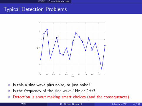
Typical Detection Problems

0 0.2 0.4 0.6 0.8 1 1.2 1.4 1.6 1.8 2−3

−2

−1

0

1

2

3

time

y(t)

Is this a sine wave plus noise, or just noise?

Is the frequency of the sine wave 1Hz or 2Hz?

Detection is about making smart choices (and the consequences).



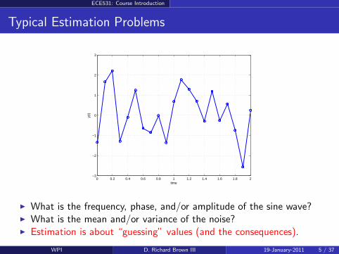
Typical Estimation Problems

0 0.2 0.4 0.6 0.8 1 1.2 1.4 1.6 1.8 2−3

−2

−1

0

1

2

3

time

y(t)

What is the frequency, phase, and/or amplitude of the sine wave? What is the mean and/or variance of the noise? Estimation is about “guessing” values (and the consequences).



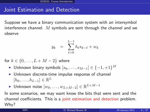
Joint Estimation and Detection

Suppose we have a binary communication system with an intersymbolinterference channel. M symbols are sent through the channel and weobserve

yk =L−1∑

ℓ=0

hℓsk−ℓ + wk

for k ∈ 0, . . . , L+M − 2 where

Unknown binary symbols [s0, . . . , sM−1] ∈ −1,+1M Unknown discrete-time impulse response of channel

[h0, . . . , hL−1] ∈ RL

Unknown noise [w0, . . . , wL+M−2] ∈ RL+M−1

In some scenarios, we may want know the bits that were sent and thechannel coefficients. This is a joint estimation and detection problem.Why?



Consequences

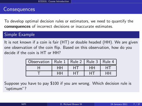
To develop optimal decision rules or estimators, we need to quantify theconsequences of incorrect decisions or inaccurate estimates.

Simple Example

It is not known if a coin is fair (HT) or double headed (HH). We are givenone observation of the coin flip. Based on this observation, how do youdecide if the coin is HT or HH?

Observation Rule 1 Rule 2 Rule 3 Rule 4

H HH HT HH HT

T HH HT HT HH

Suppose you have to pay $100 if you are wrong. Which decision rule is“optimum”?



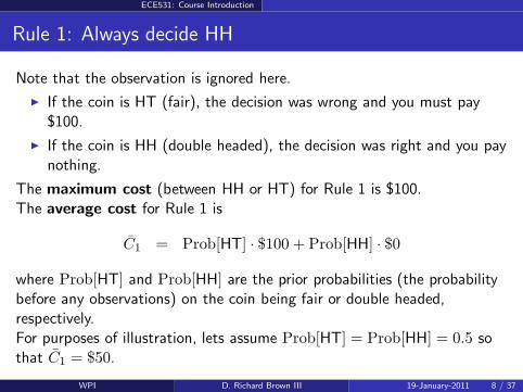
Rule 1: Always decide HH

Note that the observation is ignored here.

If the coin is HT (fair), the decision was wrong and you must pay$100.

If the coin is HH (double headed), the decision was right and you paynothing.

The maximum cost (between HH or HT) for Rule 1 is $100.The average cost for Rule 1 is

C1 = Prob[HT] · $100 + Prob[HH] · $0

where Prob[HT] and Prob[HH] are the prior probabilities (the probabilitybefore any observations) on the coin being fair or double headed,respectively.For purposes of illustration, lets assume Prob[HT] = Prob[HH] = 0.5 sothat C1 = $50.



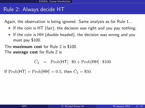
Rule 2: Always decide HT

Again, the observation is being ignored. Same analysis as for Rule 1...

If the coin is HT (fair), the decision was right and you pay nothing.

If the coin is HH (double headed), the decision was wrong and youmust pay $100.

The maximum cost for Rule 2 is $100.The average cost for Rule 2 is

C2 = Prob[HT] · $0 + Prob[HH] · $100

If Prob[HT] = Prob[HH] = 0.5, then C2 = $50.



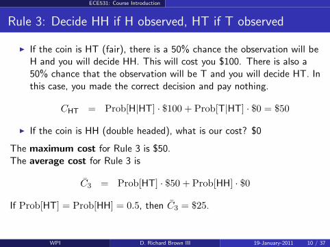
Rule 3: Decide HH if H observed, HT if T observed

If the coin is HT (fair), there is a 50% chance the observation will beH and you will decide HH. This will cost you $100. There is also a50% chance that the observation will be T and you will decide HT. Inthis case, you made the correct decision and pay nothing.

CHT = Prob[H|HT] · $100 + Prob[T|HT] · $0 = $50

If the coin is HH (double headed), what is our cost? $0


C3 = Prob[HT] · $50 + Prob[HH] · $0




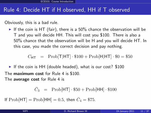
Rule 4: Decide HT if H observed, HH if T observed

Obviously, this is a bad rule.

If the coin is HT (fair), there is a 50% chance the observation will beT and you will decide HH. This will cost you $100. There is also a50% chance that the observation will be H and you will decide HT. Inthis case, you made the correct decision and pay nothing.

CHT = Prob[T|HT] · $100 + Prob[H|HT] · $0 = $50

If the coin is HH (double headed), what is our cost? $100


C3 = Prob[HT] · $50 + Prob[HH] · $100




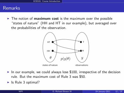
Remarks

The notion of maximum cost is the maximum over the possible“states of nature” (HH and HT in our example), but averaged overthe probabilities of the observation.

HT

HH

states of nature

T

H

observations

θ p(y|θ) y

In our example, we could always lose $100, irrespective of the decisionrule. But the maximum cost of Rule 3 was $50.

Is Rule 3 optimal?



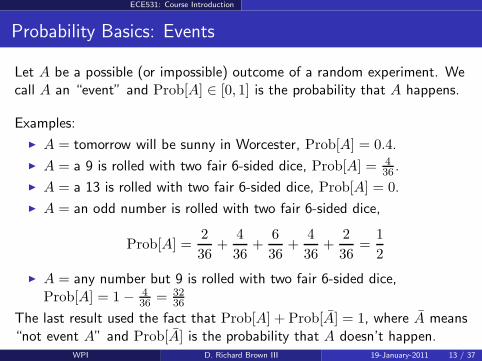
Probability Basics: Events

Let A be a possible (or impossible) outcome of a random experiment. Wecall A an “event” and Prob[A] ∈ [0, 1] is the probability that A happens.

Examples:

A = tomorrow will be sunny in Worcester, Prob[A] = 0.4.

A = a 9 is rolled with two fair 6-sided dice, Prob[A] = 4

36.

A = a 13 is rolled with two fair 6-sided dice, Prob[A] = 0.

A = an odd number is rolled with two fair 6-sided dice,

Prob[A] =2

36+

4

36+

6

36+

4

36+

2

36=

1

2

A = any number but 9 is rolled with two fair 6-sided dice,Prob[A] = 1− 4

36= 32

36

The last result used the fact that Prob[A] + Prob[A] = 1, where A means“not event A” and Prob[A] is the probability that A doesn’t happen.



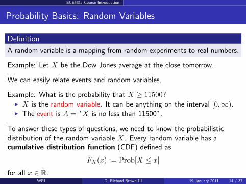
Probability Basics: Random Variables

Definition

A random variable is a mapping from random experiments to real numbers.

Example: Let X be the Dow Jones average at the close tomorrow.

We can easily relate events and random variables.

Example: What is the probability that X ≥ 11500? X is the random variable. It can be anything on the interval [0,∞). The event is A = “X is no less than 11500”.

To answer these types of questions, we need to know the probabilisticdistribution of the random variable X. Every random variable has acumulative distribution function (CDF) defined as

FX(x) := Prob[X ≤ x]

for all x ∈ R.WPI D. Richard Brown III 19-January-2011 14 / 37


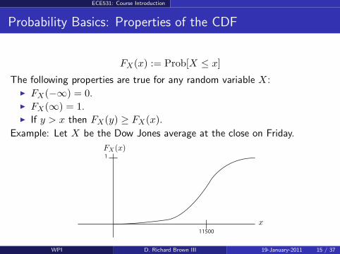
Probability Basics: Properties of the CDF

FX(x) := Prob[X ≤ x]

The following properties are true for any random variable X: FX(−∞) = 0. FX(∞) = 1. If y > x then FX(y) ≥ FX(x).

Example: Let X be the Dow Jones average at the close on Friday.

1

11500

x

FX(x)



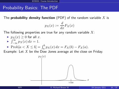
Probability Basics: The PDF

The probability density function (PDF) of the random variable X is

pX(x) :=d

dxFX(x)

The following properties are true for any random variable X: pX(x) ≥ 0 for all x.

∫

∞

−∞pX(x) dx = 1.

Prob[a < X ≤ b] =∫ ba pX(x) dx = FX(b)− FX(a).

Example: Let X be the Dow Jones average at the close on Friday.

11500

x

pX(x)



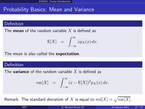
Probability Basics: Mean and Variance

Definition

The mean of the random variable X is defined as

E[X] =

∫

∞

−∞

xpX(x) dx.

The mean is also called the expectation.

Definition

The variance of the random variable X is defined as

var[X] =

∫

∞

−∞

(x− E[X])2pX(x) dx.

Remark: The standard deviation of X is equal to std[X] =√

var[X].



Probability Basics: Properties of Mean and Variance

Assuming c is a known constant, it is not difficult to show the followingproperties of the mean:

1. E[cX] = cE[X] (by linearity)

2. E[X + c] = E[X] + c (by linearity)

3. E[c] = c

Assuming c is a known constant, it is not difficult to show the followingproperties of the variance:

1. var[cX] = c2var[X]

2. var[X + c] = var[X]

3. var[c] = 0



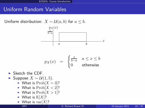
Uniform Random Variables

Uniform distribution: X ∼ U(a, b) for a ≤ b.

xa b

1

b−a

pX(x)

pX(x) =

1

b−a a ≤ x ≤ b

0 otherwise

Sketch the CDF. Suppose X ∼ U(1, 5).

What is Prob[X = 3]? What is Prob[X < 2]? What is Prob[X > 1]? What is E[X ]? What is var[X ]?



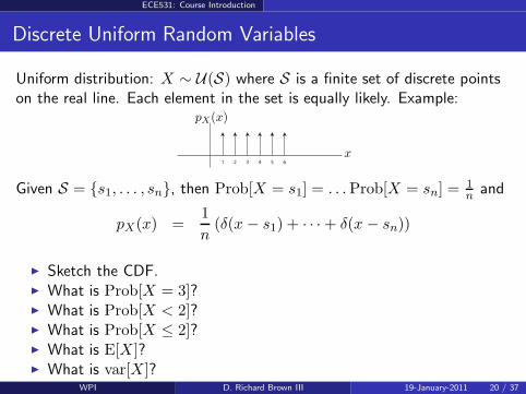
Discrete Uniform Random Variables

Uniform distribution: X ∼ U(S) where S is a finite set of discrete pointson the real line. Each element in the set is equally likely. Example:

1 2 3 4 5 6

x

pX(x)

Given S = s1, . . . , sn, then Prob[X = s1] = . . .Prob[X = sn] =1

n and

pX(x) =1

n(δ(x − s1) + · · ·+ δ(x − sn))

Sketch the CDF. What is Prob[X = 3]? What is Prob[X < 2]? What is Prob[X ≤ 2]? What is E[X]? What is var[X]?



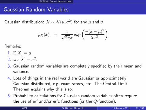
Gaussian Random Variables

Gaussian distribution: X ∼ N (µ, σ2) for any µ and σ.

pX(x) =1√2πσ

exp

(−(x− µ)2

2σ2

)

Remarks:

1. E[X] = µ.

2. var[X] = σ2.

3. Gaussian random variables are completely specified by their mean andvariance.

4. Lots of things in the real world are Gaussian or approximatelyGaussian distributed, e.g. exam scores, etc. The Central LimitTheorem explains why this is so.

5. Probability calculations for Gaussian random variables often requirethe use of erf and/or erfc functions (or the Q-function).



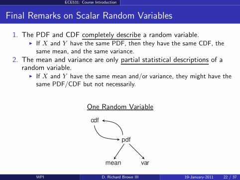
Final Remarks on Scalar Random Variables

1. The PDF and CDF completely describe a random variable. If X and Y have the same PDF, then they have the same CDF, the

same mean, and the same variance.

2. The mean and variance are only partial statistical descriptions of arandom variable.

If X and Y have the same mean and/or variance, they might have thesame PDF/CDF but not necessarily.

One Random Variable

pdf

cdf

mean var



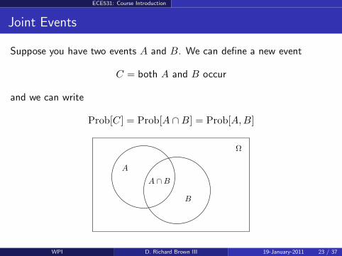
Joint Events

Suppose you have two events A and B. We can define a new event

C = both A and B occur

and we can write

Prob[C] = Prob[A ∩B] = Prob[A,B]

A

B

A ∩B

Ω



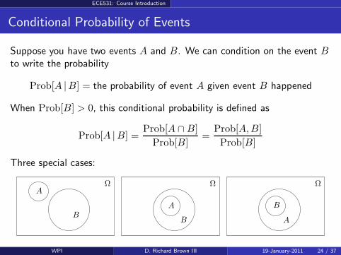
Conditional Probability of Events

Suppose you have two events A and B. We can condition on the event Bto write the probability

Prob[A |B] = the probability of event A given event B happened

When Prob[B] > 0, this conditional probability is defined as

Prob[A |B] =Prob[A ∩B]

Prob[B]=

Prob[A,B]

Prob[B]

Three special cases:

A

A

A

B

BB

ΩΩΩ



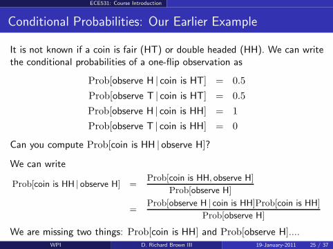
Conditional Probabilities: Our Earlier Example

It is not known if a coin is fair (HT) or double headed (HH). We can writethe conditional probabilities of a one-flip observation as

Prob[observe H | coin is HT] = 0.5

Prob[observe T | coin is HT] = 0.5

Prob[observe H | coin is HH] = 1

Prob[observe T | coin is HH] = 0

Can you compute Prob[coin is HH | observe H]?

We can write

Prob[coin is HH | observe H] =Prob[coin is HH, observe H]

Prob[observe H]

=Prob[observe H | coin is HH]Prob[coin is HH]

Prob[observe H]

We are missing two things: Prob[coin is HH] and Prob[observe H]....WPI D. Richard Brown III 19-January-2011 25 / 37


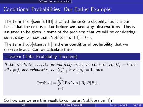
Conditional Probabilities: Our Earlier Example

The term Prob[coin is HH] is called the prior probability, i.e. it is ourbelief that the coin is unfair before we have any observations. This isassumed to be given in some of the problems that we will be considering,so let’s say for now that Prob[coin is HH] = 0.5.

The term Prob[observe H] is the unconditional probability that weobserve heads. Can we calculate this?

Theorem (Total Probability Theorem)

If the events B1, . . . , Bn are mutually exclusive, i.e. Prob[Bi, Bj ] = 0 for

all i 6= j, and exhaustive, i.e.∑n

i=1Prob[Bi] = 1, then

Prob[A] =n∑

i=1

Prob[A |Bi]P [Bi].

So how can we use this result to compute Prob[observe H]?WPI D. Richard Brown III 19-January-2011 26 / 37


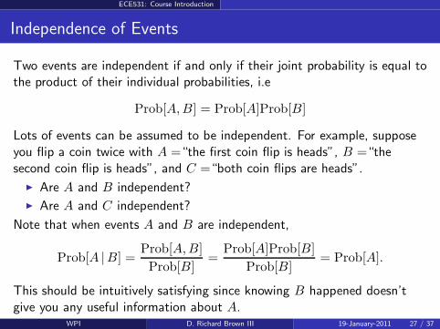
Independence of Events

Two events are independent if and only if their joint probability is equal tothe product of their individual probabilities, i.e

Prob[A,B] = Prob[A]Prob[B]

Lots of events can be assumed to be independent. For example, supposeyou flip a coin twice with A =“the first coin flip is heads”, B =“thesecond coin flip is heads”, and C =“both coin flips are heads”.

Are A and B independent?

Are A and C independent?

Note that when events A and B are independent,

Prob[A |B] =Prob[A,B]

Prob[B]=

Prob[A]Prob[B]

Prob[B]= Prob[A].

This should be intuitively satisfying since knowing B happened doesn’tgive you any useful information about A.



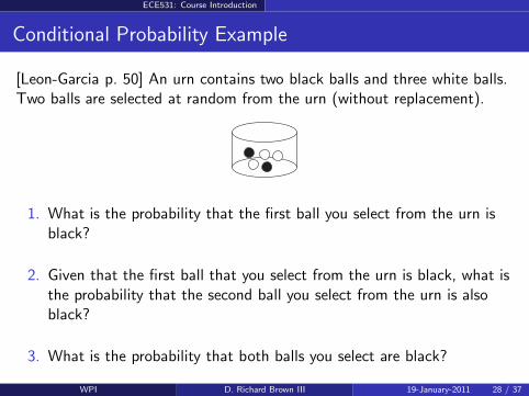
Conditional Probability Example

[Leon-Garcia p. 50] An urn contains two black balls and three white balls.Two balls are selected at random from the urn (without replacement).

1. What is the probability that the first ball you select from the urn isblack?

2. Given that the first ball that you select from the urn is black, what isthe probability that the second ball you select from the urn is alsoblack?

3. What is the probability that both balls you select are black?



Another Conditional Probability Example

An urn contains one ball known to be either black or white with equalprobability. A white ball is added to the urn, the urn is shaken, and a ballis removed randomly from the urn.

1. If the ball removed from the urn is black, what is the probability thatthe ball remaining in the urn is white?

2. If the ball removed from the urn is white, what is the probability thatthe ball remaining in the urn is white?



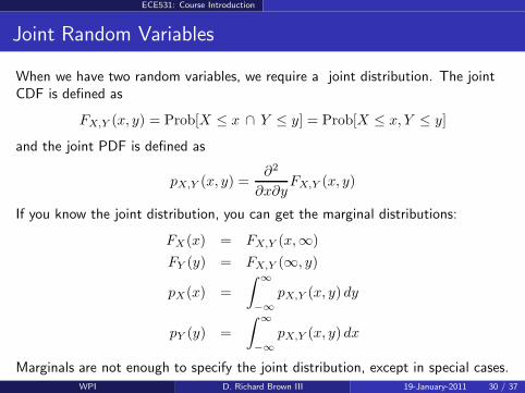
Joint Random Variables

When we have two random variables, we require a joint distribution. The jointCDF is defined as

FX,Y (x, y) = Prob[X ≤ x ∩ Y ≤ y] = Prob[X ≤ x, Y ≤ y]

and the joint PDF is defined as

pX,Y (x, y) =∂2

∂x∂yFX,Y (x, y)

If you know the joint distribution, you can get the marginal distributions:

FX(x) = FX,Y (x,∞)

FY (y) = FX,Y (∞, y)

pX(x) =

∫ ∞

−∞

pX,Y (x, y) dy

pY (y) =

∫ ∞

−∞

pX,Y (x, y) dx

Marginals are not enough to specify the joint distribution, except in special cases.WPI D. Richard Brown III 19-January-2011 30 / 37


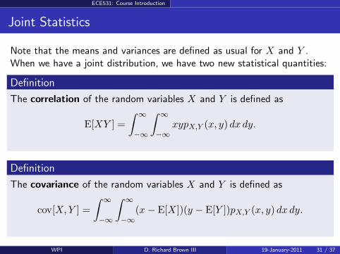
Joint Statistics

Note that the means and variances are defined as usual for X and Y .When we have a joint distribution, we have two new statistical quantities:

Definition

The correlation of the random variables X and Y is defined as

E[XY ] =

∫

∞

−∞

∫

∞

−∞

xypX,Y (x, y) dx dy.

Definition

The covariance of the random variables X and Y is defined as

cov[X,Y ] =

∫

∞

−∞

∫

∞

−∞

(x− E[X])(y − E[Y ])pX,Y (x, y) dx dy.



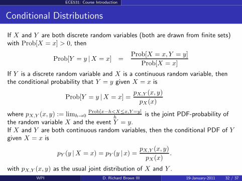
Conditional Distributions

If X and Y are both discrete random variables (both are drawn from finite sets)with Prob[X = x] > 0, then

Prob[Y = y |X = x] =Prob[X = x, Y = y]

Prob[X = x]

If Y is a discrete random variable and X is a continuous random variable, thenthe conditional probability that Y = y given X = x is

Prob[Y = y |X = x] =pX,Y (x, y)

pX(x)

where pX,Y (x, y) := limh→0Prob[x−h<X≤x,Y=y]

his the joint PDF-probability of

the random variable X and the event Y = y.If X and Y are both continuous random variables, then the conditional PDF of Ygiven X = x is

pY (y |X = x) = pY (y |x) =pX,Y (x, y)

pX(x).

with pX,Y (x, y) as the usual joint distribution of X and Y .



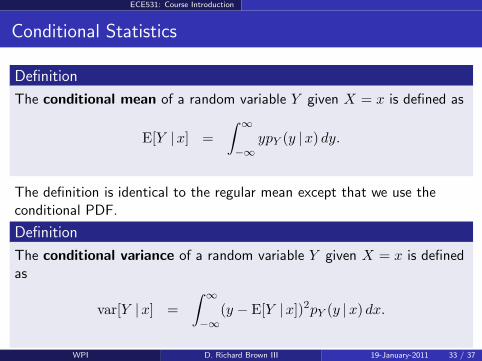
Conditional Statistics

Definition

The conditional mean of a random variable Y given X = x is defined as

E[Y |x] =

∫

∞

−∞

ypY (y |x) dy.

The definition is identical to the regular mean except that we use theconditional PDF.

Definition

The conditional variance of a random variable Y given X = x is definedas

var[Y |x] =

∫

∞

−∞

(y − E[Y |x])2pY (y |x) dx.



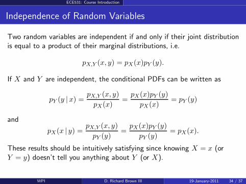
Independence of Random Variables

Two random variables are independent if and only if their joint distributionis equal to a product of their marginal distributions, i.e.

pX,Y (x, y) = pX(x)pY (y).

If X and Y are independent, the conditional PDFs can be written as

pY (y |x) =pX,Y (x, y)

pX(x)=

pX(x)pY (y)

pX(x)= pY (y)

and

pX(x | y) = pX,Y (x, y)

pY (y)=

pX(x)pY (y)

pY (y)= pX(x).

These results should be intuitively satisfying since knowing X = x (orY = y) doesn’t tell you anything about Y (or X).



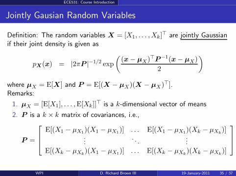
Jointly Gausian Random Variables

Definition: The random variables X = [X1, . . . ,Xk]⊤ are jointly Gaussian

if their joint density is given as

pX(x) = |2πP |−1/2 exp

(

(x− µX)⊤P−1(x− µX)

2

)

where µX = E[X] and P = E[(X − µX)(X − µX)⊤].Remarks:

1. µX = [E[X1], . . . ,E[Xk]]⊤ is a k-dimensional vector of means

2. P is a k × k matrix of covariances, i.e.,

P =

E[(X1 − µX1)(X1 − µX1

)] . . . E[(X1 − µX1)(Xk − µXk

)]...

. . ....

E[(Xk − µXk)(X1 − µX1

)] . . . E[(Xk − µXk)(Xk − µXk

)]



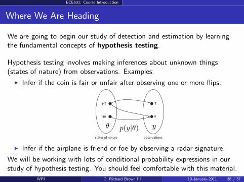
Where We Are Heading

We are going to begin our study of detection and estimation by learningthe fundamental concepts of hypothesis testing.

Hypothesis testing involves making inferences about unknown things(states of nature) from observations. Examples:

Infer if the coin is fair or unfair after observing one or more flips.

HT

HH

states of nature

T

H

observations

θ p(y|θ) y

Infer if the airplane is friend or foe by observing a radar signature.

We will be working with lots of conditional probability expressions in ourstudy of hypothesis testing. You should feel comfortable with this material.



Where We Will Be in April: Kalman Filtering

2008 Charles Stark Draper Prize: Dr. Rudolph Kalman

The Kalman Filter uses a mathematical technique that removes noise fromseries of data. From incomplete information, it can optimally estimate andcontrol the state of a changing, complex system over time. Applicationsinclude target tracking by radar, global positioning systems, hydrological

modeling, atmospheric observations, and time-series analyses ineconometrics.

(paraphrased from http://www.nae.edu/)


random variables

Documents