introduction à l’optique non-linéaire · concernent que l’interaction entre un champ et un...
TRANSCRIPT

Introduction à l’optique non-linéaire
Paul MandelUniversité Libre de BruxellesFaculté des Sciences Appliquées
(PHYS 327)
Août 2004

©2004 Paul Mandel This file contains the course Introduction to Nonlinear Optics given at the Applied Science Faculty of the Université Libre de Bruxelles during the academic year 2004-2005. Its content is copyright protected. Copies can be made by students if it is not for commercial purposes.

Contents
Preface i
I Nonlinear propagation 1
1 Two-level medium 11.1 Electric field equation . . . . . . . . . . . . . . . . . . . . . . . 11.2 Material equations . . . . . . . . . . . . . . . . . . . . . . . . 21.3 Phenomenology: incoherent pumping and decay . . . . . . . . 5
2 Propagation regimes 72.1 Linear propagation regime . . . . . . . . . . . . . . . . . . . . 72.2 Nonlinear susceptibility . . . . . . . . . . . . . . . . . . . . . . 102.3 Nonlinear steady propagation . . . . . . . . . . . . . . . . . . 132.4 Group and phase velocity . . . . . . . . . . . . . . . . . . . . 14
3 Ultrashort pulse propagation 173.1 Introduction . . . . . . . . . . . . . . . . . . . . . . . . . . . . 173.2 Self-induced transparency . . . . . . . . . . . . . . . . . . . . 173.3 Sine-Gordon equation . . . . . . . . . . . . . . . . . . . . . . . 233.4 2π solitons . . . . . . . . . . . . . . . . . . . . . . . . . . . . . 253.5 References . . . . . . . . . . . . . . . . . . . . . . . . . . . . . 27
II Cavity nonlinear optics 28
4 Laser theory 294.1 Introduction . . . . . . . . . . . . . . . . . . . . . . . . . . . . 294.2 Single mode ring laser . . . . . . . . . . . . . . . . . . . . . . 344.3 Steady states . . . . . . . . . . . . . . . . . . . . . . . . . . . 354.4 Rate equations . . . . . . . . . . . . . . . . . . . . . . . . . . 364.5 Good cavity limit . . . . . . . . . . . . . . . . . . . . . . . . . 39
i
CONTENTS ii
4.6 References . . . . . . . . . . . . . . . . . . . . . . . . . . . . . 40
5 Optical Bistability I 415.1 Introduction . . . . . . . . . . . . . . . . . . . . . . . . . . . . 415.2 Steady state solutions . . . . . . . . . . . . . . . . . . . . . . . 425.3 Optical devices . . . . . . . . . . . . . . . . . . . . . . . . . . 435.4 Generic description . . . . . . . . . . . . . . . . . . . . . . . . 455.5 Nonlinear stability . . . . . . . . . . . . . . . . . . . . . . . . 475.6 References . . . . . . . . . . . . . . . . . . . . . . . . . . . . . 495.7 Appendix: The Schmitt trigger . . . . . . . . . . . . . . . . . 50
6 Optical Bistability II 526.1 Delay-differential equations . . . . . . . . . . . . . . . . . . . . 526.2 Discrete map equations . . . . . . . . . . . . . . . . . . . . . . 536.3 Deterministic chaos . . . . . . . . . . . . . . . . . . . . . . . . 556.4 References . . . . . . . . . . . . . . . . . . . . . . . . . . . . . 59
III Weakly nonlinear systems 61
7 Frequency mixing 627.1 Tensor → vector → scalar description . . . . . . . . . . . . . . 627.2 Multiple time-scales . . . . . . . . . . . . . . . . . . . . . . . . 637.3 χ(2) media . . . . . . . . . . . . . . . . . . . . . . . . . . . . . 647.4 References . . . . . . . . . . . . . . . . . . . . . . . . . . . . . 67
8 Second harmonic generation 688.1 Formulation . . . . . . . . . . . . . . . . . . . . . . . . . . . . 688.2 Free running SHG . . . . . . . . . . . . . . . . . . . . . . . . . 708.3 Intracavity SHG . . . . . . . . . . . . . . . . . . . . . . . . . . 79
9 Sum & difference frequency generation 859.1 Sum frequency generation . . . . . . . . . . . . . . . . . . . . 85
9.1.1 Formulation . . . . . . . . . . . . . . . . . . . . . . . . 859.1.2 Free running SFG . . . . . . . . . . . . . . . . . . . . . 86
9.2 Difference frequency generation . . . . . . . . . . . . . . . . . 909.2.1 Two intense input fields . . . . . . . . . . . . . . . . . 919.2.2 One intense input field . . . . . . . . . . . . . . . . . . 92
10 Optical parametric oscillator 9510.1 Formulation . . . . . . . . . . . . . . . . . . . . . . . . . . . . 9510.2 Threshold condition . . . . . . . . . . . . . . . . . . . . . . . . 96

CONTENTS iii
10.3 Degenerate OPO . . . . . . . . . . . . . . . . . . . . . . . . . 9710.4 Ring and Fabry-Perot cavities . . . . . . . . . . . . . . . . . . 10110.5 References . . . . . . . . . . . . . . . . . . . . . . . . . . . . . 102
IV Quantum interference 103
11 Coherence and atomic interference 10411.1 Atomic interference . . . . . . . . . . . . . . . . . . . . . . . . 10411.2 Semiclassical formulation . . . . . . . . . . . . . . . . . . . . . 10711.3 Electromagnetically induced transparency (EIT) . . . . . . . . 10911.4 Slow light . . . . . . . . . . . . . . . . . . . . . . . . . . . . . 112


Préface
Le but de ces notes de cours est d’introduire l’étudiant aux notions de basede l’optique non-linéaire. Ceci implique deux aspects qu’il faut traiter si-multanément: la physique non-linéaire de l’interaction matière-lumière et lesmathématiques requises pour résoudre les équations auxquelles conduit ladescription physique des phénomènes étudiés. J’ai essayé, autant que faire sepeut, de trouver un équilibre entre ces deux aspects qui me paraissent égale-ment importants, mais il est inévitable que certains chapitres ressemblentplus à un cours de mathématiques appliquées qu’à un cours de physique, pourla bonne raison que la frontière entre ces deux disciplines est floue. On nes’étonnera donc pas de trouver de nombreux exemples de bifurcations: d’unepart, les bifurcations sont l’une des signatures naturelles des non-linéarités;d’autre part, elles sont le mécanisme de choix par lequel des solutions denouvelle nature peuvent apparaître. Typiquement, les bifurcations les plussimples décrivent l’émergence de solutions périodiques dans le temps et/oul’espace au départ d’une solution stationnaire et spatialement homogène.La base de l’optique nonlinéaire telle qu’elle est développée dans ces
notes est la théorie électromagnétique de Maxwell. C’est une théorie dif-ficile à assimiler car le champ électromagnétique est un concept unifica-teur mais abstrait1. La théorie de Maxwell est le premier exemple d’unethéorie unifiée du champ. La difficulté majeur à laquelle on se heurte est queles équations de Maxwell pour le champ électromagnétique sont linéaires,ce qui les rend conceptuellement simples, tandis que les grandeurs acces-sibles à l’expérience (énergie, intensité, puissance, . . .) sont des fonctionsbilinéaires en les champs. Contrairement à la théorie de Newton, qui ma-nipule directement les grandeurs mesurables et permet donc de formuler lesrelations fondamentales sous une forme simple (force = masse×accélération,
1Pour rappel, l’article fondateur de Maxwell A dynamical theory of the electromagneticfield est paru dans les Philosophical Transactions of the Royal Society en 1865. Un physi-cien américain, Michael Pupin, raconte qu’il est venu à Cambridge en 1883 (soit quatreans après le décès de Maxwell) pour apprendre la théorie électromagnétique et n’a trouvépersonne qui puisse l’aider. Ce n’est qu’en Allemagne, à Berlin, qu’il trouvera en H. vonHelmholtz un maître qui lui enseignera la théorie de Maxwell.
i

CONTENTS ii
action = réaction, . . .), la théorie de Maxwell manipule des champs qui véri-fient des équations aux dérivées partielles. L’ajout des relations matériellescomplique à souhait le problème. On peut voir l’optique non-linéaire commeune chronique de la stratégie développée pour transformer les équations deMaxwell en équations explicites pour des grandeurs mesurables dans le visi-ble. On retrouve le même niveau de difficulté lorsque l’on essaie d’exprimerles lois de la mécanique classique à partir de la mécanique quantique.Il est généralement impossible de déterminer les limites réelles d’un su-
jet: certaines d’entre elles paraissent si évidentes que l’on juge inutile de lesmentionner, jusqu’à ce qu’un nouveau résultat montre à quel point elles sontimportantes. L’optique non-linéaire vient d’être le sujet d’un tel bouleverse-ment. Les chapitres abordés dans les deux premières parties de ces notes neconcernent que l’interaction entre un champ et un milieu matériel qui peutêtre décrit comme un milieu à deux niveaux. Les chapitres de la troisièmepartie traitent le milieu matériel comme un milieu caractérisé par une sus-ceptibilité du deuxième ou du troisième ordre constante. Par contre, dansla quatrième partie, j’ai introduit un chapitre qui traite des phénomènesd’interférences atomiques. Actuellement, la conséquence la plus spectaculaireen est la transparence induite par voie électromagnétique et sa conséquence,la lumière lente. Il s’agit là d’un effet purement quantique puisqu’il est lié àl’aspect ondulatoire de la matière.L’optique non-linéaire souffre d’un défaut parfois considéré comme réd-
hibitoire: il n’est pas possible de la formuler au départ de principes pre-miers sans introduire des hypothèses phénoménologiques. Aussi ne me suis-je pas embarrassé de longs développements théoriques visant à justifier ceshypothèses: ces théories existent, souffrent de nombreux défauts et aboutis-sent toutes, en première approximation, au même résultat que l’approchephénoménologique.Ce cours s’articule en quatre parties complémentaires:
• La première partie est consacrée à l’étude de la propagation du champdans des systèmes fortement non-linéaires mais dont le milieu matérielpeut être décrit au moyen d’un modèle à deux niveaux.
• La deuxième partie est consacrée à l’étude des mêmes systèmes maisplacés dans des cavités résonantes.
• Dans la troisième partie, les systèmes sont faiblement non-linéaires etle milieu matériel est décrit par une polarisation atomique nonlinéairequi est une fonction bilinéaire du champ électrique.
• Enfin, la quatrième partie aborde les effets d’interférence atomique quipeuvent apparaître lorsque deux voies de désexcitation sont disponibles.

Preface iii
Le choix des chapitres développés dans ce cours résulte à la fois de lacontrainte de temps imposée à ce cours (deux modules2) et de mes centresd’intérêts. Pour une information complémentaire, l’étudiant pourra consulteravec profit les ouvrages parus sur ce sujet. Voici une brève liste de livres,récents ou classiques, qui traitent de l’optique non-linéaire:
N. Bloembergen, Nonlinear optics (Benjamin, New York, 1965).
A. Yariv and P. Yeh, Optical waves in crystals (Wiley, New York, 1984).
Y.R. Shen, The principles of nonlinear optics (Wiley, New York, 1984).
P.N. Butcher and D. Cotter, The elements of nonlinear optics (CambridgeUniversity Press, 1991).
A.C. Newell and J.V. Moloney, Nonlinear optics (Addison-Wesley, Reading,1992).
P. Mandel, Theoretical problems in cavity nonlinear optics (Cambridge Uni-versity Press, 1997).
R.W. Boyd, Nonlinear Optics 2nd Edition (Academic Press, New York,2003).
Cette liste n’est pas exhaustive. À la fin de certains chapitres, j’ai ajoutéune liste de références et/ou une bibliographie qui renvoient à des articlesoriginaux et/ou à des livres spécialisés.Finalement, un mot de précaution: dans chaque chapitre, la notation est
cohérente, mais le même symbole peut être utilisé avec des sens différentsd’un chapitre à l’autre.
2La notion de module semble relativement stable car parfaitement indéfinie. Par contre,sa traduction en terme d’heures de cours a subi des fluctuations gigantesques.


Part I
Nonlinear propagation
1


Chapter 1
Two-level medium
In this chapter, we review some properties of an electric field E interactingwith a collection of N identical two-level atoms in the semiclassical formula-tion. The purpose of this chapter is to show that a nonlinear response is therule rather than the exception in physics. However, we shall also see thatthe nonlinear response characterizing the light-matter interaction is usuallysmall. It is only in special circumstances that the nonlinear response becomesa relevant feature.
1.1 Electric field equationOur starting point is Maxwell’s equation for the electric fieldµ
∂2
∂x2− 1
c2∂2
∂t2
¶Etot =
1
ε0c2∂2ttPeff (1.1)
where Peff is the atomic polarization induced by the field Etot, c is the veloc-ity of light in vacuum and ε0 = 8.85×10⁻¹² F/m is the vacuum permittivity.All the problems which are analyzed in these lecture notes share the
property that the field will interact with active atoms embedded in a passiveand linear medium. For instance, the passive medium can be an inert buffergas needed to stabilize the active gas, it can be a solvent in which the activeliquid is diluted, or it can be the host crystal doped by the active atoms. Thetotal atomic polarization will then be the sum of the polarization generatedby the linear passive medium and the polarization, linear and nonlinear,generated by the active medium: Peff = Ppass+Pact. We may assume a lineardependence on the field Ppass = ε0χpassEtot which is the material relationneeded to close the Maxwell equation with respect to the passive medium.
1

CHAPTER 1. TWO-LEVEL MEDIUM 2Rtis assumed that the coefficient χpass is real and constant in space and time.
This leads to the field equationµv2
∂2
∂x2− ∂2
∂t2
¶Etot =
1
ε00∂2ttPact (1.2)
In this equation, the effective velocity of light in the passive medium is definedas v = c/npass ≤ c where n2pass = 1+χpass is the refractive index of the passivemedium, the permittivity ε00 = n2passε0 now refers to the passive medium andthe polarization is that of the active atoms only.We introduce the decompositions
Etot =1
2
hEei(kfx−ωf t) + c.c.
i, Pact = N
hPei(kfx−ωf t) + c.c.
i(1.3)
where the optical frequency ωf and the wave number kf are related by thedispersion relation ωf = vkf .In the absence of light-matter interaction, a solution of Maxwell’s equa-
tion is given by an electric field amplitude E which is constant in space andtime. This is no longer true, in general, in the presence of light-matter in-teraction. Therefore, we seek solutions E(x, t) which, due to the atom-fieldinteraction, vary slowly in space and time, compared with the optical spaceand time variation
ωf |P | À |∂P/∂t| , ωf |E| À |∂E/∂t| , kf |E| À |∂E/∂x| (1.4)
This is usually justified by the fact that the residual variation of the complexfield amplitude E(x, t) is related to the atomic temporal variations, whichoccur in a much longer time scale. For solid state and semiconductor mate-rials, slow atomic relaxation processes range from 1 to 10−6sec whereas fastatomic relaxation processes range from 10−6 to 10−12sec. By contrast, theoptical time scale in the visible range is about 10−14 to 10−15sec. With theseelements, it is easy to derive a propagation equation for the complex fieldamplitude
(v∂x + ∂t)E = (iNωf/ε00)P (1.5)
The final step in this derivation is to relate the polarization per atom, P ,with the microscopic properties of the medium. This is will be done in thenext section.
1.2 Material equationsThe last equation we have obtained for the electric field is still an openequation since we need a closure relation of the form P = P (E). For this,

CHAPTER 1. TWO-LEVEL MEDIUM 3
we have to introduce a model of the atomic system in order to express thereaction of the medium to the applied field. We shall assume that the mediumis a collection of N independent two-level atoms. In doing so, we thereforeassume that only resonant or, at least, quasi-resonant, interactions take place.That is, the field frequency is close to the atomic frequency (E2 −E1) /~.For each atom, the wave function is Ψ(x) = a1ϕ1(x) + a2ϕ2(x) and theHamiltonian is H = H0 + V = H0 − exEtot with the properties
i~∂Ψ
∂t= HΨ (1.6)
Ψ = a1ϕ1 + a2ϕ2 (1.7)
|a1|2 + |a2|2 = 1 (1.8)
H0ϕm = ~ωmϕm, m = 1, 2 (1.9)ZV
ϕmϕ∗ndx = δnm (1.10)
The polarization induced in each atom by the external electric field has itsorigin in the deformation of the electronic charge distribution induced bythat electric field. It is given by
p =
ZV
Ψ∗exΨdx
= a2a∗1
ZV
ϕ∗1exϕ2dx+a1a∗2
ZV
ϕ∗2exϕ1dx
≡ ex12ρ21 + ex21ρ12 (1.11)
with the standard notation for the density matrix: ρpq = apa∗q. The off-
diagonal matrix elements of the density matrix are the atomic coherence,as opposed to the atomic polarization which is the product of the atomiccoherence with the matrix element of the electric dipole moment. A coherencebetween two atomic levels p and q means that if the state of level p is modified,the level q will be affected even if the perturbation is applied only to the levelp. In systems with more than two levels, this can happen even if the matrixelement of the electric dipole between the two states vanishes (forbiddentransition). This atomic coherence should not be confused with the so-calledcoherent states of the electromagnetic field.From Schrödinger’s equation, it follows that
i~∂a1∂t
= ~ω1a1 + a1V11 + a2V12
= ~ω1a1 + a2V12
' ~ω1a1 − a2µEtot (1.12)

CHAPTER 1. TWO-LEVEL MEDIUM 4
and similarly
i~∂a2∂t
' ~ω2a2 − a1µEtot (1.13)
To derive these two equations, we have made some assumptions:
1. The interaction Hamiltonian does not have diagonal matrix elements,i.e., V11 = V22 = 0 with Onm =
Rvϕ∗nOϕmdx for any operator O.
2. The electric field Etot(x, t) does not vary significantly over an atomicdiameter. Therefore, it can be factored out in the off-diagonal matrixelements of V which can be written as V12 = −µEtot where µ = ex12 isthe dipole matrix element of the atomic transition. This approximationis known as the dipole approximation.
3. To simplify the algebra, we have assumed without loss of generalitythat µ = µ∗ since all physical quantities are functions of |µ|2 which willappear as µ2 in these notes.
From equations (1.12) and (1.13), it is easy to derive the pair of coupledequations for the bilinear functions of the coefficients ap:
∂
∂t(a2a
∗1) = −i (ω2 − ω1) a2a
∗1 + i
µ
~Etot (a1a
∗1 − a2a
∗2) (1.14)
∂
∂t(a1a
∗1) = i
µ
~Etot (a2a
∗1 − a1a
∗2) (1.15)
In the density matrix notation, these equations are written as
∂ρ21∂t
= −i (ω2 − ω1) ρ21 + iµ
~Etot (ρ11 − ρ22) (1.16)
∂ρ11∂t
= −∂ρ22∂t
= iµ
~Etot (ρ21 − ρ∗21) (1.17)
The ρpp are associated with the atomic population in level p. Defining thepopulation difference n = ρ11−ρ22 and the atomic frequency ωa = ω2−ω1 >0, we can write the evolution equations for the density matrix elements as
∂ρ21∂t
= −iωaρ21 + iµ
~Etotn (1.18)
∂n
∂t= 2i
µ
~Etot (ρ21 − ρ∗21) (1.19)
The closure relation we are looking for is
Ptot = Np (1.20)

CHAPTER 1. TWO-LEVEL MEDIUM 5
or equivalently Pei(kfx−ωf t) = µρ21 ≡ µσei(kfx−ωf t): the polarization Ptot
which induces the electric field in Maxwell’s equations is equal to the polar-ization induced by the electric field as derived from the Shrödinger equation.In doing so, we obtain a closed set of equations which couple the field andthe material variables
©Etot, ρpq
ª. This formulation of the light-matter inter-
action leads to the so-called semiclassical description since the field is treatedas classical while matter is fully quantized. Equation (1.20) results from theassumption that all atoms are identical. If the atoms differ by one or morevariables, Ptot must be expressed as the mean value over that or these vari-ables. For instance, in a gas, we must add to the energy of the atomic levels~ωp the kinetic energy of the center of mass. The total polarization thenbecomes the average over the velocity distribution g(v) which is typically agaussian or a lorentzian distribution: Ptot ∼
Rg(v)p(v)dv.
A last approximation is introduced now. This approximation is referred toas the rotating wave approximation. The left hand side of (1.18) is ∂ρ21/∂t ∼exp [i (kfx− ωf t)] while the right hand side of that equation isn
−iωaσ + iµ
2~
hE + E∗e−2i(kfx−ωf t)
inoei(kfx−ωf t). (1.21)
Likewise, the left hand side of (1.19) is ∂n/∂t while the right hand side ofthat equation is
iµ
~
hE∗σ − Eσ∗ + Eσe2i(kfx−ωf t) −E∗σ∗e−2i(kfx−ωf t)
i(1.22)
Since the field and the material variables E, σ,and n are slowly varying func-tions, we neglect fast oscillating terms proportional to exp [±2i (kfx− ωf t)],and obtain the coupled equations¡
∂x + v−1∂t¢E = (iNµωf/vε
00)σ (1.23)
∂σ
∂t= −iδσ + i
µ
2~En (1.24)
∂n
∂t= i
µ
~(E∗σ −Eσ∗) (1.25)
with δ ≡ ωa − ωf .
1.3 Phenomenology: incoherent pumping anddecay
The description obtained sofar is incomplete. Equations (1.23)-(1.25) cor-rectly describe the interaction process between stable atoms and a lossless

CHAPTER 1. TWO-LEVEL MEDIUM 6
medium. However, the atomic levels are not stable. In addition, the two-levelmodel of the medium accounts only for the quasi-resonant interaction withthe field. Apart from that, there are nonresonant interactions (involving theother atomic levels of the active atoms and/or the passive host medium)which yield a linear, i.e., field-independent loss. The usual procedure is toadd phenomenological constants to the evolution equations (1.23)-(1.25) inthe following way. For the field equation, we add to the right hand side aterm −κE ¡
∂x + v−1∂t¢E = −κE + (iNµωf/vε
00)σ (1.26)
In the absence of interaction with the two-level medium, this leads, for in-stance, to a steady solution which decays according to the Beer-Lambertlaw: E(x) = E(0) exp(−κx). The space-time dependent case in the linearapproximation will be studied in the next section.We now introduce phenomenological constants to account for the finite
life-time of the two energy levels of the active medium. For the atomicpolarization, we also add a linear damping term −γ⊥σ while the populationdifference we add the damping −γkn. However, we also have to take intoaccount incoherent processes which populate the atomic levels at differentrates. Let n0 be the population difference reached in steady state in theabsence of interaction with the coherent field Etot. Then we add a sourceterm to the population inversion evolution equation and arrive at
∂σ
∂t= −(γ⊥ + iδ)σ + i
µ
2~En (1.27)
∂n
∂t= γk(n
0 − n) + iµ
~(E∗σ −Eσ∗) (1.28)
Equations (1.26)-(1.28) form the basis of our study of two-level atoms inter-acting with a monochromatic electric field1. The set of Eqs. (1.26)-(1.28) iswidely known as the Maxwell-Bloch equations.
1In some areas, especially solid-state physics interacting with microwave radiation, thetwo relaxation times are written differently: T2 is used instead of 1/γ⊥ and T1 is usedinstead of 1/γk.

Chapter 2
Propagation regimes
2.1 Linear propagation regimeAs a first approach to Eqs. (1.26)-(1.28), we shall consider the linear regimeof propagation, in which the problem is reduced to the pair of coupled linearequations for E and σ¡
∂x + v−1∂t + κ¢E = (iNµωf/vε
00)σ (2.1)
∂σ
∂t= −(γ⊥ + iδ)σ + i
µ
2~En (2.2)
∂n
∂t= γk(n
0 − n) (2.3)
Indeed, equations (2.1)-(2.2) imply a linear relation σ ∝ E while retainingthe E-dependant term in (1.28) leads to nonlinear corrections to the relationσ ∝ E and to n.In the long time limit, we seek plane wave solutions
E = Eei(kx−ωt), σ = sei(kx−ωt), n = n0 (2.4)
The frequency ω and the wave number k which we have just introducedrepresent shifts of the unperturbed frequency ωf and wave number kf of thefield due to the atom-field interaction. Inserting (2.4) into the linearizedequations (2.1)-(2.3) leads to
(ik − iω/v + κ)E =iNωfµ
ε00vs (2.5)
−iωs = −(γ⊥ + iδ)s+iµ
2~n0E (2.6)
These are two homogeneous equations for two variables a1E + b1s = 0 anda2E + b2s = 0. The compatibility condition of this pair of homogeneous
7
CHAPTER 2. PROPAGATION REGIMES 8
equations is that the determinant of the coefficients vanishes: a1b2−a2b1 = 0,otherwise only the trivial solution E = s = 0 exists. This leads to
(k − ω/v − iκ)(ω − δ + iγ⊥) +Nωfµ
2n0
2~ε00v= 0 (2.7)
This is the dispersion relation k = k(ω) we were looking for. Its solution is
k =ω
v+
ω − δ
γ⊥α+ i(κ− α) (2.8)
α = − Nωfµ2n0
2~ε00vγ⊥£1 + (ω − δ)2/γ2⊥
¤ (2.9)
We have introduced the parameter α ∝ −n0 ≡ ρ022 − ρ011 which is the linear(or small signal) gain or loss, depending on whether it is positive or negative,respectively. The frequency detuning ω − δ = ω − ωa + ωf is the differencebetween the effective field frequency Ωf = ωf + ω and the atomic frequencyωa.The stability properties of the plane wave are easily derived from (2.8),
taking ω real:
• α < κ: In this case, Im k > 0 and the plane wave is attenuated in thelinear regime since E, σ ∼ exp [−x Im (k)].
• α > κ: In this case, Im k < 0 and the plane wave is amplified in thelinear regime.
Hence the plane wave solution is stable below the threshold α = κ andunstable above the threshold. If α > κ, there is a net gain and the lineartheory is no longer able to describe correctly the system. The importantproperty is that the gain condition α > κ can be written as a condition forthe population inversion as ρ022−ρ011 > (ρ022 − ρ011)threshold > 0. In other terms,an initial population inversion is necessary, though not sufficient, to ensuregain in the two-level medium. Note that the condition α > κ can also beinterpreted as a condition of strong light-matter interaction with µ2 > µ2crit.These questions will be studied with more details in Chapter 4.We can deduce from (2.6) the linearized eigensolution in the form of the
ratio s/E , from which we derive the expression
P
E=
µs
E =µ2n0
2~
∙ωa − Ωf
γ2⊥ + (ωa − Ωf )2+
iγ⊥γ2⊥ + (ωa − Ωf)2
¸≡ χ0(∆) (2.10)

CHAPTER 2. PROPAGATION REGIMES 9
which defines the linear susceptibility χ0 = χ00 + iχ000 with
χ00(∆) =µ2n0
2~∆
γ2⊥ +∆2(2.11)
χ000(∆) =µ2n0
2~γ⊥
γ2⊥ +∆2(2.12)
and ∆ = ωa − Ωf . The real and imaginary parts of the susceptibility arerelated by the obvious property
χ00(∆) =∆
γ⊥χ000(∆) (2.13)
From (2.1) it follows that the imaginary part of the susceptibility describesthe absorptive properties of the medium which affect the real amplitude ofthe field E. The linear gain is proportional to χ00. A way to see this pointis to decompose the field into amplitude and phase: E = |E| exp (iϕ). Thenit is easy to verify that χ00 contributes to the evolution of the amplitude |E|while χ0 contributes to the evolution of the phase ϕ:¡
∂x + v−1∂t + κ¢ |E| = −(Nωf/vε
00) |E|χ00 (2.14)¡
∂x + v−1∂t¢ϕ = (Nωf/vε
00)χ
0 (2.15)
Another way to understand the susceptibility χ is to introduce the relationP = χE into the definitions (1.3):
Ptot = NhχEei(kfx−ωf t) + c.c.
i= 2Nχ0Etot + iNχ00
hEei(kfx−ωf t) − c.c.
i≡ 2Nχ0Etot + iNχ00Ediss (2.16)
Inserting this result in the Maxwell equation (1.2) leads toÃ∂2xx −
1
v2eff∂2tt
!Etot =
iNχ00
ε00v2∂2ttEdiss (2.17)
corresponding to the propagation of a wave with velocity veff = v/n wheren =
p1 + 2Nχ0/ε00 is the refractive index of the active medium. It is ap-
parent on Eq.(2.17) that χ0 contributes to the phase evolution while χ00 con-tributes to dissipative processes since χ00 ∼ γ⊥.As a function of δ − ω = ωa − Ωf , the imaginary part χ00(ωa − Ωf) is a
Lorentzian peaked at ωa = Ωf . The real part of χ0 describes the dispersive

CHAPTER 2. PROPAGATION REGIMES 10
properties of the medium which affect the phase of the complex field ampli-tude E. It vanishes for ωa = Ωf , where χ000 is maximum. It is a characteristicof linear systems that dispersion vanishes where absorption is maximum. Thefunction g = ∆/
¡∆2 + γ2⊥
¢with ∆ = ωa − Ωf is associated with dispersion
and has extrema at ∆± = ±γ⊥ where its value is g± = ±1/(2γ⊥).The func-tion f = γ⊥/
¡∆2 + γ2⊥
¢which is associated with absorption has the property
that f(±γ⊥) = 1/(2γ⊥) at the extrema of g. A graphical representation ofthe functions f and g versus ∆ is displayed in Fig.2.1.
-10 -5 0 5 10 15
-0.3
-0.1
0.1
0.3
0.5absorption f( ∆) = γ/(∆2 +γ2) ~ χ ''
dispersion g( ∆ ) = ∆ /(∆2+γ2) ∼ χ '
∆
1/(2 γ)
Figure 2.1: Linear dispersion and absorption.
In particular, it follows from this discussion that the full width at halfmaximum (FWHM) of the absorption curve f is 2γ⊥ since the half maximumof f is reached at ∆ = ±γ⊥.Another property which is important because its validity goes well be-
yond the linear regime is the relation, on resonance (ωa = Ωf), between theimaginary part of the susceptibility and the slope of its real part:
χ000(∆ = 0) = γ⊥∂χ00(∆)∂∆
¯∆=0
(2.18)
This relation, derived from (2.13), relates the linear gain to the dispersiveproperties of the medium at the resonance.
2.2 Nonlinear susceptibilityThe nonlinear equations (1.26)-(1.28) admit steady state solutions of the form

CHAPTER 2. PROPAGATION REGIMES 11
dE/dx+ κE = (iNµωf/vε00)σ (2.19)
σ =iµ
2~En
γ⊥ + iδ(2.20)
n = n0 +iµ
~γk(E∗σ −Eσ∗) (2.21)
From the last two equations we obtain an expression of the material variablesin terms of the field intensity
n = n0
(1 +
|µE|2~2γ⊥γk[1 + (δ/γ⊥)2]
)−1(2.22)
σ = Eµn0
2~γ⊥
i+ δ/γ⊥1 + (δ/γ⊥)
2
(1 +
|µE|2~2γ⊥γk [1 + (δ/γ⊥)
2]
)−1(2.23)
Note that in the strong field limit, |E| → ∞, we have n → 0 and σ → 0.Hence we obtain
|E|→∞: ρ11 → 1/2, ρ22 → 1/2, ρ12 → 0 (2.24)
In other terms, a strong field bleaches the atomic system : n = ρ11−ρ22 → 0(which is independent of n0) but destroys the atomic coherence : ρ12 → 0.The susceptibility χ is defined by P ≡ χE; therefore the steady state
susceptibility is
χs = χ0s + iχ00s =µ2n0
2~γ⊥
i+ δ/γ⊥1 + (δ/γ⊥)
2
(1 +
|µE|2~2γ⊥γk[1 + (δ/γ⊥)
2]
)−1(2.25)
We have the obvious relation between the real and imaginary parts of thesusceptibility:
χ0 = (δ/γ⊥)χ00 (2.26)
The linear susceptibility χ0 derived in Section 2.1 is ω-dependant but field-independent. It fully characterizes the linear response of the medium to theexternal electric field via the dispersion relation k = k(ω) which originatesfrom the atom-field interaction. On the contrary, χs is the static (k = ω = 0)component of the susceptibility but it is field-dependent as no assumptionhas been made on the field amplitude. The susceptibility χs neglects theback reaction of the medium on the propagation characteristics of the field:Ωf = ωf . Both expressions represent different approximations of a more

CHAPTER 2. PROPAGATION REGIMES 12
general function which depends on ω and on the field. To make contact withthe linearized susceptibility, we write the susceptibility χs in the form
χ0s =µ2n0
2~∆eγ2⊥ +∆2
=µ2n0
2~γ⊥
∆/γ⊥
1 +K +¡∆/γ⊥
¢2 (2.27)
χ00s =µ2n0
2~r1 + |µE|2 /
³~2γ⊥γk
´ eγ⊥eγ2⊥ +∆2=
µ2n0
2~γ⊥
1
1 +K +¡∆/γ⊥
¢2 (2.28)
with eγ⊥ = γ⊥
r1 + |µE|2 /
³~2γ⊥γk
´≡ γ⊥
√1 +K (2.29)
and ∆ = ωa − Ωf . The real and imaginary parts of χs2~γ⊥/ (µ2n0) are
displayed in figure 2.2.
0.0
0.2
0.4
0.6
0.8
1.0
-10 -6 -2 2 6 10
(a) (b)
-0.6
-0.4
-0.2
0.0
0.2
0.4
0.6
-10 -6 2 6 10-2
Figure 2.2: Nonlinear dispersion and absorption as a function of ∆. (a)χ0 =Re(χ) = ∆/ (1 +K +∆2). (b)χ00 = Im(χ) = 1/ (1 +K +∆2). Units of χare µ2n0/ (2~γ⊥) . From top to bottom, K = 0, 0.5, 1, 2.5, 5 and 10.
Note that Eq. (2.18) remains valid for the nonlinear susceptibility definedby Eqs. (2.27) and (2.28). The field dependence that appears in the staticsusceptibility (2.27) and (2.28) leads to an effect which is known as powerbroadening. For instance, the FWHM is
FWHM = 2γ⊥
r1 + |µE|2 /
³~2γ⊥γk
´(2.30)
Another important effect is that the absorption, characterized by χ00, is re-
duced by a factor
r1 + |µE|2 /
³~2γ⊥γk
´from the low intensity limit: the

CHAPTER 2. PROPAGATION REGIMES 13
reduction of absorption with increasing intensity is known as saturation. Itis interesting to note that absorption and dispersion expressed in terms of eγ⊥are not modified in the same way by the light-matter interaction. However,the relation (2.18) which relates the gain and the slope of the dispersion onresonance remains true in this nonlinear regime.
2.3 Nonlinear steady propagationIn this section, we assume that the system is below its amplification threshold(α < κ). From (2.19)-(2.21) it follows that the complex field amplitude insteady state is given by
dE/dx = −κE − αEn
n0(1− iδ/γ⊥) (2.31)
α ≡ α(x, δ) =Nωfµ
2n0(x)
2~γ⊥ε00vh1 +
¡δ/γ⊥
¢2i (2.32)
We have seen in section 2.1 that n = n0 in the linear regime. Inserting thisapproximation in (2.31) and assuming that n0 is constant in space leads tothe Beer-Lambert law
|E(x)|2 = |E(0)|2 e−βx (2.33)
β = 2(κ+ α) (2.34)
where β is the linear attenuation coefficient.Coming back to the general equation (2.31), we introduce the polar de-
composition of the field E = Eeiφ in terms of which the electric field realamplitude is the solution of
dE/dx = −κE − αEn/n0 (2.35)
The reduced intensity J defined by
J =|µE|2
~2γ⊥γk[1 + (δ/γ⊥)2]
(2.36)
verifies the equation
dJ/dx = −2µκ+
α
1 + J
¶J (2.37)
The difficulty with this equation is the space-dependence of α. Let us there-fore consider the limit of negligible non resonant linear loss: κ¿ α. In that

CHAPTER 2. PROPAGATION REGIMES 14
limit, we obtain dJ/dx = −2αJ/(1 + J) which can be solved to give theimplicit equation
J − J0 + ln(J/J0) = −2Z x
0
α(x0)dx0 (2.38)
with J(0) = J0. Let us define an extinction length xext as in the lineartheory by the condition J(xext) ≡ J0e
−1. If the initial population differencen0 is space-independent, α is also space-independent and we find from (2.38)
xext =J0(1− 1/e) + 1
2α(2.39)
In the weak field limit, we have of course xext ' 1/ (2α). However, in the highintensity limit J0 À 1, we obtain xext ' J0 (1− 1/e) /2αÀ 1/ (2α). Hence,the extinction length may be significantly increased in the high field limitbecause it saturates the atomic transition and tends to bleach the materialmedium.
2.4 Group and phase velocityLet us consider again Maxwell equations for the electric field:µ
∂2
∂x2− 1
v2∂2
∂t2
¶E = 0 (2.40)
If the field propagates in vacuum, v = c. If the field propagates in a mediumwhere the polarization is related to the electric field by the material relationP = χE, the velocity appearing in Eq. (2.40) is v = c/n = c/
p1 + Re (χ),
provided χ is time-independent. In that case, we shall assume for simplicityin the following developments that χ is real. The general solution of Eq.(2.40) is E = f (t− x/v) where the function f is determined either by theboundary or by the initial conditions. Thus, the plane t−x/v = Π, where Πis constant in space and time, is a plane where the electric field is constant.In other terms, a given value of the electric field propagates at the speed v.This speed is called the phase velocity, by reference to the simplest solutionof Eq. (2.40), namely the running wave
g (t, x|k, ω) = A exp [i (kx− ωt)] = A exp [−iω (t− x/v)] (2.41)
since k = ω/v. Although the function g(x, t|k, ω) verifies the Maxwell equa-tion (2.40), it is not a physical solution since the electric field E must be real.

CHAPTER 2. PROPAGATION REGIMES 15
It is therefore at least the combination of two running waves g(x, t|k, ω) andg∗(x, t|k, ω) = g(x, t|− k,−ω).In general, the amplitude A of the running wave in Eq. (2.41) is not a
constant, but varies in space and time. Therefore, more general solutions areusually required. Their expression as a linear combination of running waveof the type (2.41) follows directly from the linearity of the equation and isthe basis of the Fourier analysis of the Maxwell equations.A less general representation is often adequate. Let us assume that, for
a particular problem, the electric field can be written as a quasi-plane wave
E(x, t) = A(x, t)ei(kx−ωt) + c.c. (2.42)
with
A(x, t) =
Z∆ω
a(ω)ei[(k−k)x−(ω−ω)t]dω (2.43)
A quasi-plane wave is a solution for which a(ω) is sharply peaked aroundthe frequency ω. It corresponds to a wave packet with frequency spread∆ω around ω. The corresponding wave number is k = ωn
¡ω, k
¢/c. In
the integral (2.43), we may expand the wave number k appearing in theexponential around k:
k = k + (ω − ω)∂k
∂ω
¯ω=ω
+O £(ω − ω)2¤
≡ k +ω − ω
vg+O £(ω − ω)2
¤(2.44)
which defines the group velocity vg of the wave packet. Therefore, the ex-pression for the field amplitude becomes
A(x, t) =
Z∆ω
a(ω)ei[(k−k)x−(ω−ω)t]dω
'Z∆ω
a(ω)e−i(ω−ω)(t−x/vg)dω (2.45)
The planes t− x/vg = Πg, where Πg is constant in space and time, move atthe group velocity vg. On Πg the amplitude of the field is constant: as a resultof the interference among the running waves with a small spread in frequency,all of them propagating at the phase velocity v, there will be an envelopeA (x, t), corresponding to a space and time localization of electromagneticenergy, which propagates at the group velocity vg.

CHAPTER 2. PROPAGATION REGIMES 16
An equation for the group velocity is easily obtained by differentiatingwith respect to k the dispersion relation kc = ωn(ω, k):
c =dω
dkn+ ω
dn
dk
= n∂ω
∂k+ ω
µ∂n
∂k+
∂n
∂ω
∂ω
∂k
¶= vg
µn+ ω
∂n
∂ω
¶+ ω
∂n
∂k(2.46)
which leads to the result
vg ≡ ∂ω
∂k=
c− ω ∂n∂k
n+ ω ∂n∂ω
(2.47)
Let us emphasize that this last result is not constrained by the linearitycondition: it is valid for any nonlinear medium for which the refractive indexis a scalar. If the medium is birefringent, the refractive index must be treatedas a vector and the group velocity must be generalized accordingly.There are two contributions to the group velocity: the first term c/ (n+ ω∂n/∂ω)
is only due to the frequency dispersion of the medium. It results fromthe fact that the refractive index varies with frequency. The second term,−ω (∂n/∂k) / (n+ ω∂n/∂ω), is proportional to the spatial dispersion of themedium. It results from the fact that the medium has a non-local responseto a probe field, i.e., that the wave packet has a finite spatial extension. Thedenominator ∂ (nω) /∂ω = n + ω∂n/∂ω ≡ ng is also known as the grouprefractive index since vg = c/ng.

Chapter 3
Ultrashort pulse propagation
3.1 IntroductionIn this chapter, we consider the propagation of short pulses in a nonlinearmedium. We know that a field of low intensity I propagating in an absorbingmedium is attenuated. Beer-Lambert’s law quantifies this property in thelinear regime by stating that the intensity varies along the propagation ofthe beam according to the law dI/dx = −CI where C is independent of Ithough it is frequency-dependent. This equation is discussed at the end ofChapter 2. In that chapter, we also derived equation (2.37) which generalizesBeer-Lambert’s law for a beam of arbitrary initial intensity propagating in anonlinear medium modelled as a two-level medium. In this chapter we shallsee how this law is modified when it is a pulse that propagates in the samenonlinear medium. To concentrate on the essential, we consider only a shortpulse. This means that the pulse duration is much shorter than any atomiccharacteristic time so that atoms can be treated as stable: the populationdifference and the atomic polarization vary only as a result of the resonantinteraction with the light pulse.
3.2 Self-induced transparencyLet us consider the propagation equation (1.23) and the material equations(1.24)-(1.25)
(v∂x + ∂t)E = (iNµωc/ε00)σ (3.1)
∂σ
∂t= −i (ωa − ωc) σ +
iµ
2~En (3.2)
∂n
∂t= i
µ
~(E∗σ − Eσ∗) (3.3)
17

CHAPTER 3. ULTRASHORT PULSE PROPAGATION 18
As a first step, we generalize these equations to account for the dispersion ofthe atomic frequency ωa. Let us assume that the medium is characterized by adistribution g(ωa) of atomic frequencies normalized to unity:
R∞0
g(ωa)dωa =1. Then Eqs. (3.1)-(3.3) become
(v∂x + ∂t)E = (iNµωc/ε00)
Z ∞
0
g(ω)σ(ω)dω (3.4)
∂σ
∂t= −i(ω − ωc)σ +
iµ
2~En (3.5)
∂n
∂t= i
µ
~(E∗σ −Eσ∗) (3.6)
where σ and n are of course functions of x, t, and ω. We decompose thecomplex electric field and polarization into real and imaginary parts
E(x, t) = E(x, t)eiφ(x,t) (3.7)
σ(ω, x, t) =1
2[Q(ω, x, t)− iP(ω, x, t)] eiφ(x,t) (3.8)
Since eiπ/2 = i, P is the quadrature of the atomic polarization which is out-of-phase with respect to the field, while Q is the quadrature of the atomicpolarization in phase with the electric field. This decomposition is physicallyrelevant since we shall see that Q contributes to the phase φ of the field andis therefore associated with the material dispersion while P is related to thevariation of the field amplitude E and is thus associated with absorption. Itfollows directly that the evolution equations are
(v∂x + ∂t) E(x, t) =Nµωc
2ε00
Z ∞
0
P(ω, x, t)g(ω)dω (3.9)
E(x, t) (v∂x + ∂t)φ(x, t) =Nµωc
2ε00
Z ∞
0
Q(ω, x, t)g(ω)dω (3.10)
∂tQ(ω, x, t) = ωc − ω − [∂tφ(x, t)]P(ω, x, t) (3.11)
∂tP(ω, x, t) = − ωc − ω − [∂tφ(x, t)]Q(ω, x, t)−(µ/~)n(ω, x, t)E(x, t) (3.12)
∂tn(ω, x, t) = (µ/~)E(x, t)P(ω, x, t) (3.13)
We shall seek solutions of these equations assuming that:
• φ(x,−∞) = 0 (initial condition),• the frequency distribution has a maximum at ωc and it is symmetricaround that maximum g(ω − ωc) = g(ωc − ω),

CHAPTER 3. ULTRASHORT PULSE PROPAGATION 19
• Q(ω, x, t) is an odd function of ω−ωc: Q(ω−ωc, x, t) = −Q(ωc−ω, x, t).This property was verified in Chapter 2: since P = (χ0 + iχ00)E ∼ σ,it follows that Q(ω − ωc, x, t) has the symmetry properties of χ0. Inthe linear theory, its expression (2.11) shows indeed that it is an anti-symmetric function of the frequency detuning. In the nonlinear theory,χ0 is also an antisymmetric function of the frequency as shown in Eqs.(2.25) and (2.26). Thus, what is assumed here is that this is a genericproperty of the susceptibility and not a mere coincidence for the modelstudied in Chapter 2.
Let us extend the lower bound of integration in the right hand side ofEq. (3.10) to −∞. Since ωc is a huge number for the optical domain (ωc ∼1014 − 1015Hz), this addition is negligible. Making this assumption implies(v∂x + ∂t)φ = 0 so that φ = f (x− vt). Assuming that the phase of thefield vanishes initially determines that f(x− vt) = 0 and therefore E is real.Hence, we are left with the equations
(v∂x + ∂t) E(x, t) =Nµωc
2ε00
Z ∞
0
P(ω, x, t)g(ω)dω (3.14)
∂tQ(ω, x, t) = (ωc − ω)P(ω, x, t) (3.15)
∂tP(ω, x, t) = − (ωc − ω)Q(ω, x, t)− (µ/~)n(ω, x, t)E(x, t)(3.16)∂tn(ω, x, t) = (µ/~)E(x, t)P(ω, x, t) (3.17)
The formal solution of the polarization equations (3.15)-(3.16) is½ P(ω, x, t)Q(ω, x, t)
¾= −(µ/~)
Z t
−∞dt0n(ω, x, t0)E(x, t0)
½cossin
¾[(ω − ωc)(t
0 − t)]
(3.18)At this point, we must recognize that it is not possible to pursue sig-
nificantly further this analysis. A useful strategy to follow in this case is toreduced the ambition of this calculation by studying a function that carriesless information. For this purpose, let us define a field area function θ through
θ(x, t) = (µ/~)Z t
−∞E(x, t0)dt0 (3.19)
or equivalently ∂tθ(x, t) = (µ/~)E(x, t) and a parametera = N |µ|2 ωc/(2~ε00v) (3.20)
The function θ is the area under the pulse up to time t. It is a kind of partialaverage. This function plays a dominant role in this chapter because it is thatfunction which verifies a simple propagation equation.

CHAPTER 3. ULTRASHORT PULSE PROPAGATION 20
We integrate the field equation (3.14) with respect to t and multiply itby µ/~ to get
(v∂x + ∂t) θ(x, t) = −av(µ/~)Z ∞
0
g(ω)ψ(ω, x, t)dω (3.21)
ψ(ω, x, t) =
Z t
−∞dt0Z t0
−∞dt00n(ω, x, t00)E(x, t00) cos [(ω − ωc)(t
00 − t0)] (3.22)
This last equation can be transformed as follows
ψ(t) =
Z t
−∞dt0Z t0
−∞dt00f(t00) cos [(ω − ωc)(t
00 − t0)]
=1
ωc − ω
Z t
−∞dt0Z t0
−∞dt00f(t00)∂t0 sin [(ω − ωc)(t
00 − t0)]
=1
ωc − ω
Z t
−∞dt0∂t0
Z t0
−∞dt00f(t00) sin [(ω − ωc)(t
00 − t0)]
=
Z t
−∞f(t0)
sin [(ω − ωc)(t− t0)]ω − ωc
dt0 (3.23)
To progress one step further, we consider the long time limit t → +∞ anduse the property
limt→+∞
sin(αt)
α= πδ(α) (3.24)
to study the equation that determines the evolution of the total area underthe pulse θ(x) = θ(x,+∞)
dθ(x)/dx = −a(µ/~)Z ∞
0
dωg(ω)
Z +∞
−∞n(ω, x, t)E(x, t)πδ(ω − ωc)dt
= −πa(µ/~)g(ωc)
Z +∞
−∞n(ωc, x, t)E(x, t)dt (3.25)
Comparing equations (3.21) and (3.25), we conclude that all atoms of themedium contribute to the time evolution of the partial field envelope θ(x, t)but that only the resonant atoms, for which ωa = ωc, contribute to thetotal field envelope. This remark has far reaching consequences. The atomicdynamics on resonance is governed by the pair of equations
∂P∂t
= −(µ/~)En (3.26)
∂n
∂t= (µ/~)EP (3.27)

CHAPTER 3. ULTRASHORT PULSE PROPAGATION 21
which is a conservative system since ∂t (P2 + n2) = 0. Hence, P2(x, t) +n2(x, t) = n2(x) where n(x) is the population difference before the pulseinteracts with the medium. If the lower energy level of the medium is morepopulated than the upper energy level, n(x) > 0 and the medium is anabsorber. If the upper energy level of the medium is more populated thanthe lower energy level, n(x) < 0 and the medium is an amplifier. The solutionof (3.26)-(3.27) is
P(x, t) = −n(x) sin θ(x, t) (3.28)
n(x, t) = n(x) cos θ(x, t) (3.29)
and therefore the equation for the total pulse area is
dθ(x)/dx = πag(ωc)
Z +∞
−∞dt∂tP(x, t)
= −πag(ωc)n(x) sin θ(x) (3.30)
Equation (3.30) is known as the McCall & Hahn theorem1. Its derivationand experimental verification was the subject of Sam McCall’s Ph.D. thesisunder the supervision of Hahn.Let us analyze some properties of this equation which we rewrite in the
form
dθ(x)/dx = α sin θ(x) (3.31)
α = −Nπµ2ωcn
2~ε00vg(ωc) (3.32)
In the low intensity limit, θ ¿ 1, we can approximate the sine function byits argument. This leads to the linear equation dθ(x)/dx = αθ(x) which is avariation on Beer-Lambert’s law, as should be. This limit also tells us that1/α is the absorption length in the small signal limit.The new features brought in by the nonlinear treatment of the light-
matter interaction is the occurrence of non trivial stationary solutions. In-deed, it is clear that θ = nπ is a family of solutions of the McCall & Hahnequation (3.31). The existence of non trivial stationary solutions is not pos-sible in the linear theory: in the low intensity regime, this family of solutionis reduced to θ = 0 which is of little interest. However, at higher intensity,non trivial steady state solutions exist due to the nonlinear response of themedium to the field. This means that under suitable conditions, a medium
1S.L. McCall and E.L. Hahn, Phys. Rev. Lett. 18 (1967) 908; Phys. Rev. 183 (1969)457; Phys. Rev. A2 (1970) 861.

CHAPTER 3. ULTRASHORT PULSE PROPAGATION 22
which is absorbing at low intensity2 becomes transparent and the pulse prop-agates without attenuation. This phenomenon is called self-induced trans-parency (SIT) because it is the pulse itself which bleaches the medium. Weshall elucidate in Section 3.3 the dynamical aspect of this unexpected prop-erty.The existence of a solution θ = nπ does not guarantee its stability. Let us
therefore consider infinitesimal deviations from the stationary solution: θn =nπ+ εΘn(x)+O(ε2). In the remainder of this chapter, we shall assume thatn, and therefore α, is constant in space. Inserting this solution into (3.31)and linearizing the resulting equation with respect to ε leads to dΘn/dx =Θnα cos(nπ). It follows that the solution Θn is stable iff α cos(nπ) < 0. Wecan therefore classify the stable solutions in two classes:
• for an attenuator (α < 0) the stable solutions are n = 0, 2, 4, . . .
• for an amplifier (α > 0) the stable solutions are n = 1, 3, 5, . . .
The general solution of equation (3.31) is
tanθ(x)
2= eαx tan
θ(0)
2(3.33)
Let us analyze this solution in more details. Let us consider an initial con-dition θ(0). There exists a non-negative integer n such that nπ ≤ θ(0) ≤(n+ 1)π.
• For an attenuator, the pulse area θ(x) decreases until it reaches thelower bound nπ if n is even; it increases until it reaches the upperbound (n+ 1)π if n is odd. Practically, the bounds are reached after afew absorption lengths 1/α.
• For an amplifier, the pulse area θ(x) decreases until it reaches the lowerbound nπ if n is odd; it increases until it reaches the upper bound(n+ 1)π if n is even.
2This absorption can be very strong, leading to a completely opaque medium at lowintensity.

CHAPTER 3. ULTRASHORT PULSE PROPAGATION 23
θ(x)
absorptionamplification
4π
2π
3π
π
αx-2.5 -1.5 -0.5 0.5 1.5 2.5
Figure 3.1: Steady state pulse area as a function of the propagation distance.
This discussion of the solutions is summarized in Fig. 3.1 When discussingthe pulse propagation and reshaping, it should be borne in mind that thepulse envelope θ(x, t) is not related in any simple way to the field energy andeven less to energy conservation. In fact, multiplying equation (3.14) by Eand using equation (3.17) yields the law of energy variation
∂t
µE2(x, t)− ~ωc
ε00N
Z ∞
0
g(ω)n(ω, x, t)dw
¶+ v∂xE2(x, t) = 0 (3.34)
Thus there is no inconsistency in the fact that a medium with all the atomsin the lower state cannot transfer any energy to the field and the fact that ifthe pulse is characterized by θ(x = 0) = π + ε with 0 < ε ¿ 1 it will reachθ(x) = 2π for long distances.
3.3 Sine-Gordon equationWe have seen that a inhomogeneous broadened medium (i.e., a medium inwhich there is a distribution of atomic frequencies g(ω) which is not a deltafunction) the phenomenon of SIT may take place. In the previous section, wehave provided a first analysis of this phenomenon by considering the spatialvariation of the total field envelope. Although all atoms contribute to the fieldenvelope θ(x, t) given by equations (3.21)-(3.22), we have seen from equation(3.25) that only the resonant atoms (δ = ω− ωc = 0) contribute to the totalenvelope θ(x). Therefore, we shall study in this section the dynamics of thelight field interacting only with those atoms which are on resonance with theelectric field optical carrier frequency ωc. This will describe the dynamicsthat leads, asymptotically, to the properties of θ(x).Starting from equations (3.1)-(3.3) with δ = 0, we may then assume that
the polarization is purely imaginary and that µ is real. Defining 2iσ = s, we

CHAPTER 3. ULTRASHORT PULSE PROPAGATION 24
write equations (3.1)-(3.3) in the form
(v∂x + ∂t)E = (Nµωc/2ε00)s (3.35)
∂s
∂t= − (µ/~)En (3.36)
∂n
∂t= (µ/~)Es (3.37)
As we have already noticed, there is an invariant s2(x, t) + n2(x, t) = C(x).Let n(x) be the population difference in the absence of electric field (i.e., fort = −∞). The solution of the two material equations is given by (3.28) and(3.29). Using the property ∂θ/∂t = (µ/~)E, it is now easy to derive a closedequation for θ : µ
v∂
∂x+
∂
∂t
¶∂θ
∂t= −Nµ2ωcn(x)
2ε00~sin θ (3.38)
To obtain one of the canonical forms of this equation, we introduce the changeof variables
ξ = Ωx/v, τ = Ω(t− x/v), Ω2 = Nµ2ωc |n| /2~ε00 (3.39)
in terms of which equation (3.38) becomes
∂2θ
∂τ∂ξ= ± sin θ (3.40)
The minus sign corresponds to an attenuator (n > 0), the plus sign corre-sponds to an amplifier (n < 0). We have made the assumption that themedium is homogeneous (∂n/∂x = 0) to simplify somewhat the analytic dis-cussion which follows. Equation (3.40) is known as the sine-Gordon equation.It is a highly nonlinear equation describing the propagation of a short pulsein a nonlinear medium.The sine-Gordon equation is not a newcomer in mathematics or physics.
It was found at the end of the XIXth century by mathematicians workingon differential geometry of surfaces with constant negative curvature suchas the sphere. A good account of this aspect of the sine-Gordon is foundin the classic book of Eisenhart3. It has also been derived in the context ofdislocation theory, model field theories, and superconductivity4.
3L.P. Eisenhart, A treatise on the differential geometry of curves and surfaces (Dover,New York, 1960).
4See the review by G.L. Lamb, Rev. Mod. Phys. 43 (1971) 99 for further references onthese topics.

CHAPTER 3. ULTRASHORT PULSE PROPAGATION 25
A fascinating property of the sine-Gordon equation is that analytical so-lutions can be derived in a systematic way, though not all solutions areaccessible analytically. For the simplest class of non trivial solutions, the 2πsolitons, only the Bäcklund theorem is needed to generate analytic solutions.For the higher order solutions, the Bianchi theorem is also needed. Its proofand applications are found in the complements to this chapter.
Theorem 1 The Bäcklund transformation.Let θ0 and θ1 be two functions which are related by the so-called Bäcklund
transformations
∂
∂τ
θ1 − θ02
= a sinθ1 + θ02
(3.41)
∂
∂ξ
θ1 + θ02
= ±1asin
θ1 − θ02
(3.42)
The Bäcklund theorem states that the functions θ0 and θ1 are solutions of thesine-Gordon equation.
Proof. The proof is elementary: deriving the first equation with respectto ξ and the second with respect to τ leads to a pair of equations whosedifference is the sine-Gordon equation for θ0 and whose sum is the sine-Gordon equation for θ1.The interest of this theorem is that it reduces the discussion of a second
order PDE to a pair of first order PDE’s: if a solution θ0 is known, finding asecond solution requires only two quadratures. The relevance of this theoremis that θ0 = 0 generates via the Bäcklund transformations an infinite sequenceof solutions.
3.4 2π solitonsAn obvious solution of the sine-Gordon is θ0 = 0. Using the Bäcklund trans-formation with the parameter a1 real, we find that, for an attenuator, asolution θ1 is given by
∂θ1/∂τ = 2a sin(θ1/2), ∂θ1/∂ξ = −(2/a) sin(θ1/2) (3.43)
From these two equations it follows that ∂θ1/∂(aτ) + ∂θ1/∂(ξ/a) = 0 andtherefore there exists a solution θ1 which depends on a single variable θ1 =f(aτ − ξ/a) ≡ f(ρ). This solution is |tan (θ1/4)| = exp(ρ). Hence, we have
(µ/~)E1 = ∂tθ1 = (2/w)sech [(t− x/v1) /w] (3.44)
v1 = v/(1 + 1/a2), w = 1/aΩ (3.45)
CHAPTER 3. ULTRASHORT PULSE PROPAGATION 26
This solution describes a pulse which is a localized solution peaked at t =x/v1, moving at the speed v1 which is always smaller than v, with a maximumof 2/w and a full width at half maximum of 2w ln
¡2 +√3¢ ' 2.6339w ≈
8w/3. Indeed, the function f(z) = (2/τ)sech(z/τ ) is maximum at z =0 where f(0) = 2/τ . Hence at half maximum we have f(z∗) = 1/τ =(2/τ)sech(z∗/τ) or 1 = 4 [exp (z∗/τ ) + exp (−z∗/τ)]−1 and therefore y2 −4y+1 = 0 with y = exp (z∗/τ). Thus, the one-parameter family of solutionsf(z) has the property that the product of the maximum by the full widthat half maximum is the constant 4 ln
¡2 +√3¢. In addition, the propagation
speed is proportional to the width of the pulse: given two pulses verifying(3.44)-(3.45), the pulse with larger maximum will have the smaller width andthe smaller velocity.This solution is known as a 2π soliton because the total area under the
field envelope is 2π :
θ1(x) = (µ/~)Z +∞
−∞E1(x, t)dt = 2π (3.46)
In other terms, the soliton (3.44) we have just constructed corresponds tothe 2π solution of the McCall and Hahn (3.31).No analytic expression is available for the stable solutions in an ampli-
fier because the basic π solution verifies the third Painlevé transcendentalequation, which is known only as an infinite series.The physics of the 2π soliton is easily understood in terms of the result
n(x, t) = n(x) cos θ(x, t):
1. The leading edge of the pulse interacts with the medium in such away that the first quarter of the pulse, for which θ(x, tπ/2) = π/2,leaves the system in the state n(x, tπ/2) = 0: there are exactly as manyatoms in the upper and in the lower state and therefore the medium istransparent to the radiation.
2. The second quarter of the pulse inverses the medium since at tπ definedby θ(x, tπ) = π we have n(x, tπ) = −n(x).
3. The third quarter of the pulse restores transparency at t3π/2 sinceθ(x, t3π/2) = 3π/2 implies n(x, t3π/2) = 0.
4. Finally, the last quarter of the pulse brings the system back to its initialstate n(x, t2π) = n(x) with t2π defined by θ(x, t2π) = 2π.
The interesting property is that this analysis holds irrespective of theinitial population difference n(x), provided n(x) 6= 0.

CHAPTER 3. ULTRASHORT PULSE PROPAGATION 27
3.5 References1. G.L. Lamb, Elements of soliton theory (Wiley, New York, 1960).
2. G. Eilenberger, Solitons (Springer, Heidelberg, 1981).
3. R.K. Dodd, J.C. Eilback, J.D. Gibbon, and M.C. Morris, Solitons andnonlinear wave equations (Academic Press, New York, 1982).
4. W. Eckhaus and A. van Harten, The inverse scattering transformationand the theory of solitons (North Holland, Amsterdam, 1983).
5. S. Novikov, S. Marakov, and L. Pitaevski, Theory of solitons (Consul-tant Bureau, New York, 1984).
6. M. Lakshmanan, Solitons (Springer, Heidelberg, 1988).
7. P.G. Drazin and R.S. Johnson, Solitons: an introduction (CambridgeUniversity Press, 1989).
8. A. Hasegawa, Optical solitons in fibers (Springer, Heidelberg, 1989).
9. M. Remoissenet, Waves called solitons (Springer, Heidelberg, 1994).


Part II
Cavity nonlinear optics
28


Chapter 4
Laser theory
4.1 IntroductionIn the previous chapters, we have described examples of light-matter interac-tion and nonlinear propagation. A completely different problem arises if thenonlinear medium is placed inside a resonant cavity. This was first realizedin the microwave domain (typically cm wavelengths), developed for radarapplications, where cavities having the dimensions of the wavelength to beamplified were easily constructed. The idea is to use a cavity in which the fieldcan resonate. That is, if the cavity is a rectangular volume of sides Lx, Ly, Lz
it supports modes φ(x, y, z) = φ(x)φ(y)φ(z) where φ(r) =√2 sin (krr) with
wave numbers kr = ±nrπ/Lr, r being any of the three coordinates and nran integer. In maser cavities, this number is typically 1 or 2. Only modes ofthe field which are cavity eigenmodes would be amplified, the other modesbeing strongly damped. According to the results of Chapter 2, amplificationrequires an inversion of population of the two energy levels.The extension of this technique to the optical domain was hampered by
several problems, among which:
• in the optical domain such a cavity would have linear dimensions ofthe order of 10−6 m and a precision of the order of 0.1% would mean aprecision of 10−9m = 10 angstroms or about 10 atoms;
• in such a cavity, the amount of matter that can be inserted would makegain hardly possible;
• The spontaneous emission coefficient given by Einstein’s A coefficientA = 2ω3a |µ|2 / (3hε00c3) is generally larger in the optical domain thanin the microwave domain because of the ω3 factor. Is it possible tomaintain a population inversion long enough to generate gain?
29

CHAPTER 4. LASER THEORY 30
The solution was proposed simultaneously in Russia by Basov and Prokhorovand in the US by Schawlow and Townes. The trick is to use a Fabry-Perotinterferometer as resonant cavity and exploit spontaneous emission to trig-ger the field amplification process as follows. The Fabry-Perot resonator isa volume limited longitudinally by two mirrors characterized by their reflec-tivity (which is a sensitive function of the optical frequency). In the case oflasers, it is customary not to have lateral reflecting boundaries. A nonlinearmedium is selected because its spectrum has a pair of energy levels, betweenwhich a transition is allowed, and whose frequency difference matches aneigenfrequency of the Fabry-Perot. In addition, the upper of the two levelshas to be metastable, i.e., as long lived as possible while the lowest of thetwo levels should be highly unstable, i.e., as short lived as possible. This isnot the prevailing situation in spectroscopy but pairs of level matching theseconditions can be found. The following sequence of processes takes place.
• An external source of energy, usually in the form of incoherent lightor electric discharge, is used to create a population inversion betweenthe two energy levels which have been selected. Alternative choicesof incoherent sources being used are chemical reactions and inelasticcollisions between gases.
• This leads to a field created by spontaneous emission associated totransitions from the upper to the lower levels. Its characteristics is tohave a broad frequency distribution, typically a Lorentzian distribution,peaked around the atomic frequency and having a FWHM given by theinverse of the upper level atomic life time. In addition, the wave vectorsare evenly distributed in all space directions.
• The cavity, which on purpose does not have reflecting lateral bound-aries, selects in a purely geometric way wave vectors which are parallelto the resonator axis. Field components with other wave vectors quicklyescape the cavity via the lateral boundaries. In addition, the cavity alsoselects photons whose frequency matches a cavity frequency.
• Stimulated emission now begins, in which a photon, whose frequencyand wave vector have been selected by the cavity, interacts with theamplifying medium to produce a second photon with the same phaseand, in particular, the same frequency and wave vector. In order toachieve amplification, the stimulated emission must compensate theinverse process, i.e., absorption. This requires that the stimulated gainα defined by Eq. (2.9) be positive, which imposes that a population

CHAPTER 4. LASER THEORY 31
inversion be created between the two levels involved in the atomic tran-sition.
As a result of this sequence of processes, it appears that the spontaneousemission is essential to trigger the lasing process but it yields only a weakfield. On the contrary, the stimulated field will have an intensity that growsproportionally to itself, i.e., an exponential growth which builds up fromthe weak spontaneous field. Hence the acronym laser which stands for LightAmplification by Stimulated Emission of Radiation. Finally, the balancebetween loss, gain, and saturation determines a finite intensity regime.It is quite clear that the model for light-matter interaction which we have
built in the first chapter fits nicely into the picture just described: it accountsfor all the elements which have been described in the lasing process except forthe spontaneous field because the field studied in Chapter 1 is not quantized.Since the spontaneous field is needed only in the short time limit to triggerstimulated amplification, we may use a model that neglects the quantumvacuum which produces the spontaneous emission and replace it by a post-initial condition which introduces that field into the picture. In doing so, weneglect the spontaneous contribution to the linewidth, which in any case issharply reduced by the filtering action of the interferometer. As a result, wemodel the laser by means of the equations
(v∂x + ∂t)E = −κE + (iNµωc/ε00)σ (4.1)
∂σ
∂t= −(γ⊥ + iδ)σ − i
µ
2~En (4.2)
∂n
∂t= γk(n
0 − n)− iµ
~(E∗σ −Eσ∗) (4.3)
where n = n2 − n1 is now the atomic population inversion and n0 > 0. Thefrequency ωc is a cavity eigenfrequency. Given the definition (1.3) of thecomplex field and polarization amplitudes as coefficients of running waves,this model applies to a ring laser. It is a configuration in which the lightfollows a closed path, such as a triangular or a Z shape. There is an outputmirror with reflectivity less than unity. All other mirrors are assumed tobe fully reflecting. The damping rate κ can easily be expressed in termsof more accessible parameters of the laser. Let the material medium becharacterized by an intensity absorption coefficient αBL (Beer-Lambert’s law)and a refractive index nr, while the cavity, of length L, is limited by a mirrorof intensity reflectivity R < 1, the other mirrors being perfectly reflecting(R = 1). In the absence of a nonlinear medium, Eq. (4.1) yields for theintensity loss per cavity round-trip
I(x, t+ τ)/I(x, t) = e−2κL/v = e−2κnrL/c = Re−αBLL (4.4)

CHAPTER 4. LASER THEORY 32
from which we obtain
κ =c
2nr
∙αBL +
1
Lln (1/R)
¸(4.5)
This expression of the loss coefficient contains two parts:
• cαBL/ (2nr) which accounts for the linear losses of any medium placedinside the cavity, such as the medium which serves as a support for thedoping (i.e., active) atoms in a solid state laser, or the buffer gas in agas laser, for instance.
• [c/ (2Lnr)] ln (1/R) which accounts for the losses due to the mirrors.
In the limit R→ 1, we obtain the expression
κ ' c
2nr
µαBL +
1−R
L
¶(4.6)
In some cases, mirrors may even be unnecessary. If the lasing mediumis a crystal or a dopant embedded in a crystal, the difference between therefractive indices of the crystal and of the surrounding medium (usually air)provides a reflection coefficient which is given in the linear approximation bythe Fresnel formula
R =
µn1 − n2n1 + n2
¶2(4.7)
This expression is valid under normal incidence. For instance, InSb is asemiconductor at room temperature with a refractive index n = 4 in thevisible and near infrared. This leads to R = 0.36 if we take n1 = 1 andn2 = 4. Thus a crystal cut along crystallographic facets is a natural, poorbut cheap, cavity. The crystal of YAG used in the Nd:YAG laser has arefractive index n2 = 1.6. This yields R = 0.0533, which is too small. Hence,this laser will need external mirrors.A cavity can easily support many modes. For instance the Nd ion in a
YAG (yttrium aluminum garnet) matrix, which constitutes a standard solidstate laser, has a set of allowed transitions between the 4F3/2 doublet andthe 4I11/2 manifold. Widely used transitions around 1060nm are shown inFig. 4.1. Cavity modes have frequencies given by ωcav = pπc/nrL where pis an integer. Thus, two consecutive cavity modes are separated by ∆ω =πc/ (nrL). Using the definition λω = 2πv = 2πc/nr, we find ∆ω = ω1 −ω2 = 2πc/ (nrλ1)− 2πc/ (nrλ2) = 2πc∆λ/ (nrλ1λ2) where nr is the Nd:YAGrefractive index. This gives ∆λ = λ1λ2/ (2L) ' λ21/ (2L). Therefore ∆λ '

CHAPTER 4. LASER THEORY 33
4I11/2(5) at 2473 cm-1
4I11/2(6) at 2526 cm-1
4I11/2(4) at 2146 cm-1
4I11/2(2) at 2029 cm-1
4F3/2(2) at 11502 cm-1 (R2)
4F3/2(1) at 11484 cm-1 (R1)
Nd (in YAG) spectrum
4I11/2(3) at 2111 cm-1 (Y3)
4I11/2(1) at 2001 cm-1 (Y1)
Figure 4.1: Allowed transitions visible on the fluoresence spectrum of theNd:YAG between 1050 and 1080nm at 300C. The R2 — Y3 transition has thelowest lasing threshold at 300C.
0.0532nm and ∆ω ' 9.4 × 10⁹Hz for the transition at 1064.14nm with arefractive index of 1.6 and a cavity of 1 cm. Since γ⊥ ' 1012Hz in thismedium, up to 106 cavity modes could oscillate on each of these atomictransitions unless special care is taken to have the laser operating singlemode. The usual solid state lasers have typical lengths of 1 to 10 cm and thecavity mode spacing will therefore be 1 to 10 times smaller so that 1 to 10times more modes may oscillate simultaneously.The selection of the lasing frequency strongly depends on the properties of
the cavity mirrors and on the temperature. For instance, the usual setup forNd:YAG lasers promotes lasing at 1064.14nm (R2 → Y3 transition), the mostcommonly used of the Nd lines at room temperature. At low temperature,it is the R1 → Y1 transition at 1061.52nm which has the lowest threshold.However, a different coating can easily be made which promotes the transitionbetween the same 4F3/2(2) upper level and a level of the 4I13/2(2) manifold,with an atomic frequency at 1320.0nm (R2 → X2 transition). The followingtable gives the dominant transitions observed at room temperature in thefluorescence spectrum. The Yn label the energy levels of the 4I11/2 manifold

CHAPTER 4. LASER THEORY 34
while the Xn label the energy levels of the 4I13/2 manifold (from Solid-StateLaser Engineering by Walter Koechner, Springer Verlag, 1996).
wavelength (nm) transition relative amplitude1064.14 R2 → Y3 1001061.52 R1 → Y1 921073.8 R1 → Y3 651064.6 R1 → Y2 ∼501112.1 R2 → Y6 491052.05 R2 → Y1 461115.9 R1 → Y5 461122.6 R1 → Y6 401078.0 R1 → Y4 341318.8 R2 → X1 341338.2 R2 → X3 241335.0 R1 → X2 151356.4 R1 → X4 141333.8 R1 → X1 131320.0 R2 → X2 91105.4 R2 → Y5 91341.0 R2 → X4 9
4.2 Single mode ring laserIn this section, we concentrate on the properties of a single mode laser ina ring geometry, that is, a resonator of length L where the mirrors (threeof them at least) are placed such that light follows a closed path. Thisamounts to assume that the cavity eigenmodes are φ(x) = L−1/2 exp (ikx)where k = ±2nπx/L and n is an integer. Equations (4.1)-(4.3) were derivedfor such a cavity. In the single mode regime, we may seek solutions with∂E/∂x = 01. Another simplification comes from the assumption that onecavity frequency ωc matches the atomic frequency ωa. In that case, δ = 0and we may seek solutions such that E is real and σ purely imaginary. Thus
dE
dt= −κE + (iNµωc/ε
00)σ (4.8)
dσ
dt= −γ⊥σ − i
µ
2~En (4.9)
1These are not the only single cavity mode solutions. Another class of solutions consistsof a pulse train along the longitudinal cavity optical axis. See H. Risken and K. Nummedal,J. Appl. Phys. 39 (1968) 4662 and R. Graham and H. Haken, Z. Physik 213 (1968) 420.
CHAPTER 4. LASER THEORY 35
dn
dt= γk(n
0 − n)− i2µ
~Eσ (4.10)
Finally, the change of variables
E =
s~2γ⊥γkµ2
E , σ = −in0
2
rγkγ⊥P , n = n0D (4.11)
leads to the set of reduced equations
dEdt= −κ (E −AP) (4.12)
dPdt= −P + ED (4.13)
dDdt= γ (1−D − EP) (4.14)
where we have introduced the dimensionless gain coefficient
A =Nn0µ2ωc
2~ε00κγ⊥> 0 (4.15)
and the reduced time and decay rates
t ≡ γ⊥t, γ = γk/γ⊥, κ = κ/γ⊥ (4.16)
The definition of A is such that A > 0 if there is population inversion. Theparameter A is related to the linear gain α defined in Chapter 2, equation(2.9), by the relation A = vα/κ.
4.3 Steady statesLet us analyze the steady state properties of the laser. Since Ω is the lasingfrequency, the steady state field is dEs/dt = 0, corresponding to a constantintensity. From this it follows that P and D are also independent of time.The steady state properties of the laser are given by the solutions of thealgebraic equations
Es −APs = 0 (4.17)
Ps − EsDs = 0 (4.18)
Ds = 1− EsPs (4.19)

CHAPTER 4. LASER THEORY 36
Eliminating the two material variables Ps and Ds from (4.18) and (4.19)leads to
Ds =1
1 + E2s, Ps =
1
1 + E2sEs (4.20)
and the equation for the electric field becomes
Esµ1− A
1 + E2¶= 0 (4.21)
There are two possible solutions:
1. The trivial solution Es = Ps = D − 1 = 0;2. The non-trivial solution Es 6= 0 for which
E2 = A− 1, Ps = Es/A, Ds = 1/A (4.22)
The lasing threshold condition is thus A = vα/κ = 1. It is again acondition expressing a balance between gain (vα) and losses (κ) as derivedin Section (2.1) of the first chapter.
4.4 Rate equationsIn most lasing materials, the atomic polarization is by far the fastest decayingprocess. This means γ⊥ À γk and γ⊥ À κ. Let us show that in this limit thelaser equations can be reduced to a simpler set of evolution equations. Webegin with equations (4.12)-(4.14) and introduce a small parameter ε = κ ≡κ/γ⊥. We also specify the ratio γk/γ⊥ = O(ε) = εa1 + ε2a2 + . . . ≡ εa(ε)with a1 6= 0. Note that a = γk/ (εγ⊥) = γk/κ. The laser equations become
dEdt= −ε (E −AP) (4.23)
dPdt= −P + ED (4.24)
dDdt= aε (−D + 1− EP) (4.25)
In the limit ε = 0, we have dE/dt = dD/dt = 0 and dP/dt = −P+ED whichexpresses the fact that on the time scale t = γ⊥t only the atomic polarizationevolves while the field and the population inversion do not vary. This is notthe information we seek, but it suggests that we rather look for a solution of

CHAPTER 4. LASER THEORY 37
the laser equations (4.23)-(4.25) depending on the time scale εt = κt ≡ tκ.We easily obtain
dEdtκ
= − (E − AP) (4.26)
−P + ED = εdPdtk
' 0 (4.27)
dDdtκ
= a (−D + 1− EP) (4.28)
These equations express the dynamics of the slow variables E and D on thetime scale tκ and the relation between the atomic polarization and the slowvariables at the same time: P(tκ) = E(tκ)D(tκ). This algebraic relationneglects the fast transients that occur on the time scale t = tκ/ε. Thisproperty is illustrated in Fig. 4.2 where a qualitative representation of thedeviation from steady state is plotted versus time. It should be stressed
0.00 0.05 0.100.0
0.2
0.4
0.6
0.8
1.0
P(t)
D(t), E(t)
(a)
0.0 0.5 1.0 1.5 2.0 2.5 3.00.0
0.2
0.4
0.6
0.8
1.0
(b)
D(t), E(t)
P(t)
Figure 4.2: The functions exp (−x) and exp (−100x) are displayed using twodifferent time scales to exemplify the difference between the time scales t andtκ.
that, by definition, the function D(tκ) ≡ P(tκ)/E(tκ) is also the nonlinearsusceptibility of the medium. The dynamical equations are
dEdtκ
= E (−1 +AD) (4.29)
dDdtκ
= a¡−D + 1−DE2¢ (4.30)
From the field equation we easily derive an equation for the intensity E2
dE2dtκ
= 2E2 (−1 +AD) (4.31)

CHAPTER 4. LASER THEORY 38
Finally, defining the intensity I = E2, the pumping rate w = A, the ratioeκ = κ/γk, the scaled population inversion D = wD and using the timeet = atκ = γkt, the laser equations become
dI
det = 2eκI (D − 1) (4.32)
dD
det = w −D (1 + I) (4.33)
Equations that relate the population dynamics directly either to the electricfield amplitude (as in Eqs. (4.29)-(4.30)) or to the electric field intensity(as in Eqs. (4.32)-(4.33)) are known as the rate equations. In the version(4.32)-(4.33), they describe the laser in terms of a “population dynamics”that couples the number of photons and the number of inverted atoms. Arelevant property of the rate equations is that they do not allow for a Hopfbifurcation. More precisely, the value AH of the pump parameter at which theHopf appears moves to infinity in the rate equation limit. The source termw in the equation for the population inversion is known as the optical pumpparameter. It models the balance of all the incoherent processes that lead toa population inversion in steady state and in the absence of interaction withthe field. The lasing threshold occurs at w = 1 and there is lasing for w > 1.Let us stress that although the approach presented here is the usual pro-
cedure, known as the adiabatic elimination of the fast variables, an omissionhas been made which may constitute a serious mistake. To derive equations(4.23)-(4.25), we have assumed the existence of well-defined relations amongthe decay rates: κ/γ⊥ = ε and γk/γ⊥ = O(ε). This is of course insuffi-cient. To derive equations (4.23)-(4.25) we have to specify all the orders ofmagnitude: we have in fact assumed implicitly that the dynamical variablesE ,P, and D and the parameter A are O(ε0). Under these conditions, equa-tions (4.23)-(4.25) are indeed valid. A physical counterexample is the limitA = O(1/ε) realized in the cryogenic hydrogen maser which is described bythe laser equations2. It can be shown3 that for this range of parameters, thesteady state is not stable, but the intensity is a periodic function with a largeamplitude maximum (∼ 1/ε) of short duration separated by a long domainof vanishingly small intensity [∼ exp (−1/ε)]. In that situation, two differentscalings, instead of one, are needed to describe the dynamical variables and
2A.C. Maan, H.T.C. Stoof, B.J. Verhaar and P. Mandel, Phys. Rev. Lett. 64 (1990)2630; P. Mandel, A.C. Maan, B.J. Verhaar and H.T.C. Stoof, Phys. Rev. A 44 (1991)608.
3K.A. Robbins, SIAM J. Appl. Math. 36 (1979) 457; A.C. Fowler and M.J. McGuin-ness, Physica 5D (1982) 149.

CHAPTER 4. LASER THEORY 39
the relevant time scales. This situation requires a more elaborate mathemat-ical treatment. This periodic solution may undergo successive bifurcationsleading to deterministic chaos.The importance of the rate equations stems from the fact that generally
they are the adequate level of description for many solid state lasers if thelaser is subjected to an external constraint. Among the classic situations,let us mention the periodic modulation of either gain or cavity losses, theinfluence of an external feedback loop, the injected signal to mode- or phase-lock the laser.
4.5 Good cavity limitThere is a class of lasers, such as the Ar+ laser, for which a further simplifica-tion is possible. These lasers are characterized by the fact that the materialvariables, atomic polarization and population inversion, decay much fasterthan the field inside the cavity. That is, we have γ⊥ ' γk, but γ⊥ À κ andγk À κ. It turns out that the analysis of the previous section can be extendedto cover the good cavity limit without much difficulty by simply taking thelimit a = γk/κ = O(ε). From equations (4.26)-(4.28) we obtain
dEdtκ
= − (E − AP) (4.34)
0 = −P + ED (4.35)
0 = −D + 1− EP (4.36)
Solving the last two equations to express P and D in terms of E leads to asingle equation for the complex field
dEdtκ
= Eµ−1 +A
1
1 + E2
(4.37)
From this equation we derive an evolution equation for the field intensityI = E2
dI
dτ= I
µ−1 + A
1 + I
¶(4.38)
where τ = 2tκ = 2κt. Close to threshold, for I ¿ 1, the so-called cubicapproximation4 may be used as well
dI
dτ= I [−1 +A (1− I)] (4.39)
which can be solved exactly if the pump parameter A is a constant.4The expression cubic approximation comes from early analyses of this equation which
was expressed in terms of the field amplitude rather in terms of intensity.

CHAPTER 4. LASER THEORY 40
4.6 ReferencesBooks on resonators
1. G. Hernandez, Fabry-Perot interferometers (Cambridge University Press,1986).
2. J.M. Vaughan, The Fabry-Perot interferometer (A. Hilger, Bristol,1989).
3. N. Hodgson and H. Weber, Optical resonators (Springer, Heidelberg,1997).
Books on lasers
1. H. Haken, Encyclopedia of physics (V.XXV/2C) Genzel ed. (Springer,Heidelberg, 1970).
2. M. Sargent III, M.O. Scully, and W. Lamb Jr., Laser physics (Addison-Wesley, Reading 1974).
3. H. Haken, Light vol.1 & 2 (North-Holland, Amsterdam, 1981).
4. A.E. Siegman, Lasers (University Science Books, Mill ValleyMA, 1986).
5. J. Hecht, Understanding lasers (IEEE Press, New York, 1988).
6. P.M. Milonni and J.H. Eberley, Lasers (Wiley, New York, 1988).
7. O. Svelto, Principles of lasers (Plenum, New York, 1989).
8. L. Mandel and E. Wolf, Optical coherence and quantum optics (Cam-bridge University press, 1995).
9. W.T. Silfast, Laser fundamentals (Cambridge University Press, 1996).
10. G. Grynberg, A. Aspect, and C. Fabre, Introduction aux lasers et àl’optique quantique (Editions Ellipses, Paris, 1997).
11. D. Dangoisse, D. Hennequin, and V. Zehnlé-Dhaoui, Les lasers (Dunod,Paris, 1998).

Chapter 5
Optical Bistability I
5.1 IntroductionIn Chapter 4, we have studied properties of lasers, that is, nonlinear resonantcavities in which incoherent pumping induces a population inversion. In thischapter, we analyze a variant of this set-up by considering what happens ifthe nonlinear cavity is driven by a coherent source such as another laser andthe nonlinear medium is not brought to a state of population inversion. Sucha device is known under the generic name of optically bistable device and theassociated phenomenon is known as optical bistability (OB) because for thisclass of devices the output intensity versus input intensity displays a hys-teresis and therefore a domain of bistability. Most studies of OB have beenmotivated by applications to all-optical digital signal processing. Althoughthis technology is not yet ripe for industrial applications, an intermediatestep is the realization of electro-optical devices which are now close to in-dustrial production. Device applications motivate the selection of topics inthis chapter, but the last part will be devoted to more fundamental questionsrelated to deterministic chaos.The formulation of OB follows the pattern traced in the previous chapters.
Starting for instance with Eqs. (4.12)-(4.14), we add a source term Ei to thefield equation to account for the coherent driving of the nonlinear ring cavity.This leads to the set of coupled equations
dE
dt= −κ (E + 2CP−Ei) (5.1)
dP
dt= −P + ED (5.2)
dD
dt= γ (1−D −EP ) (5.3)
41

CHAPTER 5. OPTICAL BISTABILITY I 42
where 2C = Nn0µ2ωc/ (2~ε00κγ⊥), n0 = n011 − n022 > 0, ωa = ωc = ωi
where ωi is the frequency of the driving (or input) field. In the absence ofa nonlinear medium and on resonance, the steady solution is E = Ei whichgives Ei =
√TEinput where Einput is the driving field outside the cavity
and T is the field intensity transmission coefficient of the incoupling mirror.The output field is the fraction of the cavity field that escapes the cavitythrough the outcoupling mirror. It is a linear function of the cavity fieldamplitude. Because of this, the two fields are often not distinguished inphysical discussions. Finally, the time and decay rate scaling is t = γ⊥t,κ = κ/γ⊥, and γ = γk/γ⊥.
5.2 Steady state solutionsLet us first consider the steady state solutions of equations (5.1)-(5.3)
D = 1/¡1 + E2
¢(5.4)
P = E/¡1 + E2
¢(5.5)
Ei = E + 2CE/¡1 + E2
¢(5.6)
The electric field amplitude E is the solution of a cubic equation and theremay be either one or three real solutions. The three classes of solutions aredisplayed in Fig. 5.1.
C > C critC = C crit
C < C crit
Ei
E
Figure 5.1: Cavity field amplitude versus input field amplitude.
We see that there is a critical value of C such that for C < Ccrit thesystem is monostable, i.e., the cubic (5.6) has only one real root whereas forC > Ccrit the system is bistable, i.e., the cubic (5.6) has a domain where the

CHAPTER 5. OPTICAL BISTABILITY I 43
three roots are real. For this reason the parameter C is usually referred toas the bistability parameter. Let us determine this critical value. From (5.6)it follows that
dE/dEi =¡1 + E2
¢/¡3E2 − 2EEi + 1 + 2C
¢(5.7)
At the limit points, which exist only in the bistable domain, the derivativedE/dEi is infinite, which implies 3E2−2EEi+1+2C = 0. The two solutionsof this equation are
E± =1
3
µEi ±
qE2i − 3 (1 + 2C)
¶(5.8)
Thus the domain of existence for bistability is bounded by E+ = E− = Ecrit,or equivalently 3Ecrit = Ei,crit and E2
i,crit = 3 (1 + 2Ccrit). Combining theserelations with the steady state equation (5.6) leads to
Ccrit = 4, Ecrit =√3, Ei,crit = 3
√3 (5.9)
At that point, there is a unique point with vertical slope. For C . Ccrit,the device has the properties of an optical transistor and may be used assuch. For C > Ccrit the simultaneous solution of the steady state equation(5.6) and the condition for vertical slope 2EEi = 1 + 2C + 3E2 leads toE4± + 2 (1− C)E2
± + 1 + 2C = 0 whose solutions are
E2+ = C − 1 +
pC (C − 4), E2
− =1 + 2C
C − 1 +pC (C − 4) (5.10)
In the domain C > Ccrit, there is an hysteresis which implies jump transitionsbetween the two branches as the input field as varied across the limit points.This is displayed in Fig. 5.2.
5.3 Optical devicesThe hysteresis displayed by the input/output characteristics of OB suggeststo exploit the system as a binary memory. Consider the device being drivenby an external field Ei = E1 in the bistable domain: E− < E1 < E+. If thedevice has reached that state starting below the lower limit point E− andincreasing the driving field amplitude, the cavity field is on the lower branch,corresponding to a weak cavity field amplitude and to an even weaker trans-mitted or output field amplitude. If the driving field Ei is increased beyondthe limit point E−, the device will follow the bistable curve until E− and
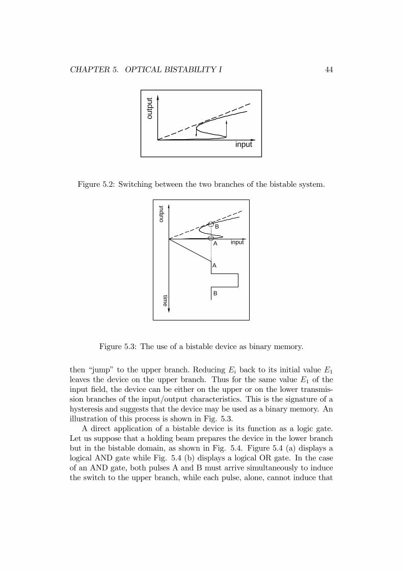
CHAPTER 5. OPTICAL BISTABILITY I 44
inputou
tput
Figure 5.2: Switching between the two branches of the bistable system.
outp
ut
inputtim
e
A
A
B
B
Figure 5.3: The use of a bistable device as binary memory.
then “jump” to the upper branch. Reducing Ei back to its initial value E1leaves the device on the upper branch. Thus for the same value E1 of theinput field, the device can be either on the upper or on the lower transmis-sion branches of the input/output characteristics. This is the signature of ahysteresis and suggests that the device may be used as a binary memory. Anillustration of this process is shown in Fig. 5.3.A direct application of a bistable device is its function as a logic gate.
Let us suppose that a holding beam prepares the device in the lower branchbut in the bistable domain, as shown in Fig. 5.4. Figure 5.4 (a) displays alogical AND gate while Fig. 5.4 (b) displays a logical OR gate. In the caseof an AND gate, both pulses A and B must arrive simultaneously to inducethe switch to the upper branch, while each pulse, alone, cannot induce that
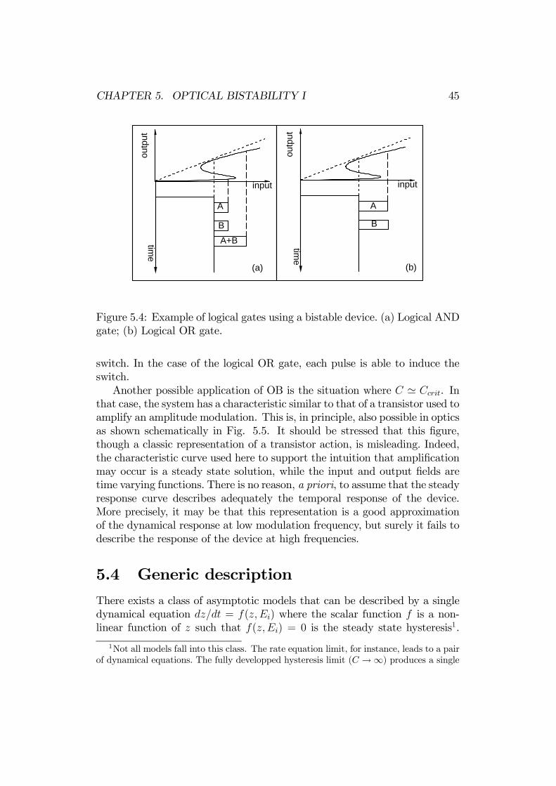
CHAPTER 5. OPTICAL BISTABILITY I 45
(a) (b)
input
outp
ut
time
A
B
A+B
input
outp
ut
time
A
B
Figure 5.4: Example of logical gates using a bistable device. (a) Logical ANDgate; (b) Logical OR gate.
switch. In the case of the logical OR gate, each pulse is able to induce theswitch.Another possible application of OB is the situation where C ' Ccrit. In
that case, the system has a characteristic similar to that of a transistor used toamplify an amplitude modulation. This is, in principle, also possible in opticsas shown schematically in Fig. 5.5. It should be stressed that this figure,though a classic representation of a transistor action, is misleading. Indeed,the characteristic curve used here to support the intuition that amplificationmay occur is a steady state solution, while the input and output fields aretime varying functions. There is no reason, a priori, to assume that the steadyresponse curve describes adequately the temporal response of the device.More precisely, it may be that this representation is a good approximationof the dynamical response at low modulation frequency, but surely it fails todescribe the response of the device at high frequencies.
5.4 Generic descriptionThere exists a class of asymptotic models that can be described by a singledynamical equation dz/dt = f(z, Ei) where the scalar function f is a non-linear function of z such that f(z,Ei) = 0 is the steady state hysteresis1.
1Not all models fall into this class. The rate equation limit, for instance, leads to a pairof dynamical equations. The fully developped hysteresis limit (C →∞) produces a single

CHAPTER 5. OPTICAL BISTABILITY I 46
output
inpu
t
Figure 5.5: Use of a optical nonlinear device close to the bistable domain asan optical transistor.
Let us exclude from the following discussion the domain C . Ccrit whichis the optical transistor. Then the function f has two limit points and thevicinity of the limit point is unambiguously defined. In the vicinity of eachlimit point, the function f(z, Ei) may be approximated locally by a parabolawhich coincides with f(z,Ei) right at the limit point. We then make a changeof variables such that the new coordinates of the limit point are (1, 1). Letx be the rescaled dynamical variable (proportional to the cavity field, andtherefore also proportional to the output field), µ the rescaled input field andτ the rescaled time. The orientation of the parabola is fixed by the furtherrequirement that the coefficient of x2 be ±1. This procedure leads to genericequations, i.e., different physical processes and/or systems are described bythe same equation. Figure 5.6 shows graphically this procedure.The relevance of a reduced description is that in device applications based
on switching between the two branches, one tries hard to prepare and main-tain the device as close as possible to the limit point. The generic characterof the local description around the limit points has been proved experimen-tally: the prediction of the generic equations have been confirmed by meansof an electric circuit (Schmitt trigger), optically bistable devices (2 mm-thickinterference filters and the 192m-long bistable device of Lille university) andbistability in Na vapor. The function f was different in each of these exam-ples. The case of the Schmitt trigger is discussed in the Appendix to thischapter.
dynamical equation, but for a different variable near each limit point and the function fdoes not reduce to the full bistable curve in steady state.
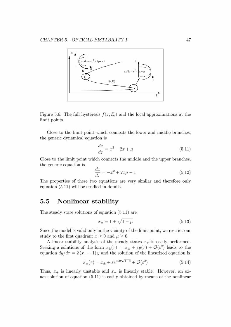
CHAPTER 5. OPTICAL BISTABILITY I 47
µ
Ei
x
x
f(z,Ei)
µ
dx/dτ = - x 2 + 2 µx - 1
dx/dτ = x 2 - 2x + µ
Figure 5.6: The full hysteresis f(z,Ei) and the local approximations at thelimit points.
Close to the limit point which connects the lower and middle branches,the generic dynamical equation is
dx
dτ= x2 − 2x+ µ (5.11)
Close to the limit point which connects the middle and the upper branches,the generic equation is
dx
dτ= −x2 + 2xµ− 1 (5.12)
The properties of these two equations are very similar and therefore onlyequation (5.11) will be studied in details.
5.5 Nonlinear stabilityThe steady state solutions of equation (5.11) are
x± = 1±p1− µ (5.13)
Since the model is valid only in the vicinity of the limit point, we restrict ourstudy to the first quadrant x ≥ 0 and µ ≥ 0.A linear stability analysis of the steady states x± is easily performed.
Seeking a solutions of the form x±(τ) = x± + εy(τ) + O(ε2) leads to theequation dy/dτ = 2 (x± − 1) y and the solution of the linearized equation is
x±(τ ) = x± + εe±2τ√1−µ +O(ε2) (5.14)
Thus, x+ is linearly unstable and x− is linearly stable. However, an ex-act solution of equation (5.11) is easily obtained by means of the nonlinear
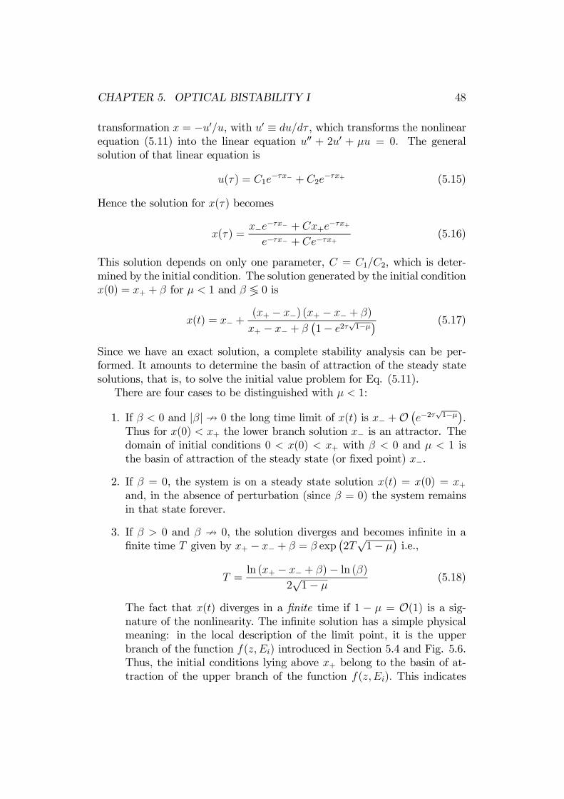
CHAPTER 5. OPTICAL BISTABILITY I 48
transformation x = −u0/u, with u0 ≡ du/dτ , which transforms the nonlinearequation (5.11) into the linear equation u00 + 2u0 + µu = 0. The generalsolution of that linear equation is
u(τ ) = C1e−τx− + C2e
−τx+ (5.15)
Hence the solution for x(τ) becomes
x(τ ) =x−e−τx− + Cx+e
−τx+
e−τx− + Ce−τx+(5.16)
This solution depends on only one parameter, C = C1/C2, which is deter-mined by the initial condition. The solution generated by the initial conditionx(0) = x+ + β for µ < 1 and β ≶ 0 is
x(t) = x− +(x+ − x−) (x+ − x− + β)
x+ − x− + β¡1− e2τ
√1−µ¢ (5.17)
Since we have an exact solution, a complete stability analysis can be per-formed. It amounts to determine the basin of attraction of the steady statesolutions, that is, to solve the initial value problem for Eq. (5.11).There are four cases to be distinguished with µ < 1:
1. If β < 0 and |β|9 0 the long time limit of x(t) is x− +O¡e−2τ
√1−µ¢.
Thus for x(0) < x+ the lower branch solution x− is an attractor. Thedomain of initial conditions 0 < x(0) < x+ with β < 0 and µ < 1 isthe basin of attraction of the steady state (or fixed point) x−.
2. If β = 0, the system is on a steady state solution x(t) = x(0) = x+and, in the absence of perturbation (since β = 0) the system remainsin that state forever.
3. If β > 0 and β 9 0, the solution diverges and becomes infinite in afinite time T given by x+ − x− + β = β exp
¡2T√1− µ
¢i.e.,
T =ln (x+ − x− + β)− ln (β)
2√1− µ
(5.18)
The fact that x(t) diverges in a finite time if 1 − µ = O(1) is a sig-nature of the nonlinearity. The infinite solution has a simple physicalmeaning: in the local description of the limit point, it is the upperbranch of the function f(z, Ei) introduced in Section 5.4 and Fig. 5.6.Thus, the initial conditions lying above x+ belong to the basin of at-traction of the upper branch of the function f(z,Ei). This indicates
CHAPTER 5. OPTICAL BISTABILITY I 49
that the middle branch of the function f(z, Ei) is unstable close tothe limit points. By continuity, we may infer the instability of thewhole middle branch. Furthermore, if µ is close to the limit point,the switching time T diverges as (1− µ)−1/2 or, in physical variables,as [(Ei,lim − Ei) /Ei,lim]
−1/2. This divergence near a limit point is knownas critical slowing down. The same phenomenon occurs in the vicinityof the laser first threshold, for the same reason though with a differentexponent. The difference in the exponent is related to the differencein the nature of the critical points: bifurcation for the laser and limitpoint in optical bistability.
4. If |β| ¿ 1 and 1− µ = O(1), another singularity of the switching timeappears
T =ln (1/β)
2√1− µ
+O(1) (5.19)
This is another case of slowing down, known as non critical slowingdown, characterized by a logarithmic divergence.
What is important to note here is that in both cases of slowing down,the divergence is related to a degeneracy: critical slowing down occurs neara limit point where two solutions of f(z,Ei) coincide, non critical slowingdown occurs near the critical line or separatrix (x+) separating two basins ofattraction, of x = x− and of x =∞. Critical slowing down can also be under-stood in the following way. The linear stability analysis yields the eignevalueλ = 2
√1− µ. This defines a time scale τ = 1/λ = 1/2
√1− µ. Close to
the limit point, λ → 0 which implies that the characterisitc relaxation timeτ →∞. Thus critical slowing down is associated with the degenerate situa-tion that defines the limit point: two solutions of a single ordinary differentialequation coincide at that point. This degeneracy induces the vanishing of atleast one eignevalue which, in turn, mean the divergence of a characterisitctime.
5.6 ReferencesOptical bistability
1. L.A. Lugiato, Theory of optical bistability, Progress in Optics vol. XXI,E. Wolf ed. (North Holland, Amsterdam, 1984), 71-216.
2. S.D. Smith, Optical bistability, photonic logic and the optical computer,Phil. Trans. R. Soc. London A 313 (1984) 187-451.
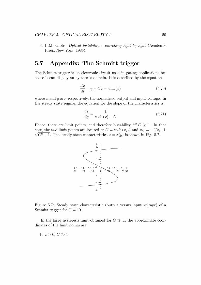
CHAPTER 5. OPTICAL BISTABILITY I 50
3. H.M. Gibbs, Optical bistability: controlling light by light (AcademicPress, New York, 1985).
5.7 Appendix: The Schmitt triggerThe Schmitt trigger is an electronic circuit used in gating applications be-cause it can display an hysteresis domain. It is described by the equation
dx
dt= y + Cx− sinh (x) (5.20)
where x and y are, respectively, the normalized output and input voltage. Inthe steady state regime, the equation for the slope of the characteristics is
dx
dy=
1
cosh (x)− C(5.21)
Hence, there are limit points, and therefore bistability, iff C ≥ 1. In thatcase, the two limit points are located at C = cosh (xM) and yM = −CxM ±√C2 − 1. The steady state characteristics x = x(y) is shown in Fig. 5.7.
-6
-4
-2
0
2
4
6x
-30 -20 -10 0 10 20 30y
Figure 5.7: Steady state characteristic (output versus input voltage) of aSchmitt trigger for C = 10.
In the large hysteresis limit obtained for C À 1, the approximate coor-dinates of the limit points are
1. x > 0, C À 1
CHAPTER 5. OPTICAL BISTABILITY I 51
Since C = cosh (xM) ' (1/2) exp (xM), the coordinates of that limitpoint are
xM ' ln (2C) > 0
yM ' C [1− ln (2C)] < 0yM + CxM = +
√C2 − 1 (5.22)
2. x < 0, C À 1
Since C = cosh (xM) ' (1/2) exp (−xM), the coordinates of that limitpoint are
xM ' − ln (2C) < 0yM ' −C [1− ln (2C)] > 0
yM + CxM = −√C2 − 1 (5.23)
Let us now consider the evolution equation in the vicinity of the limitpoint (xM , yM) with xM < 0 and yM > 0:
dx
dt= y + Cx−
"sinh (xM) + (x− xm) cosh (xM) +
(x− xM)2
2sinh (xM) + . . .
#
= y + Cx−"−√C2 − 1 + (x− xM)C − (x− xM)
2
2
√C2 − 1 + . . .
#
' x2
2
√C2 − 1− xxM
√C2 − 1 +
µy − yM +
x2M2
√C2 − 1
¶(5.24)
We define the parameters
α = − |xM | , β = −2|xM |
√C2 − 1 (5.25)
and the scaled variablesx = αz, t = βτ (5.26)
Inserting these definitions in Eq. (5.24) leads to the canonical form
dz
dτ= z2 − 2z + µ (5.27)
where
µ = 1− 2 (y − yM)
x2M√C2 − 1 ≤ 1 (5.28)


Chapter 6
Optical Bistability II
Apart from its potential for applications in all-optical signal processing, op-tical bistability has also been a source of inspiration for studies in nonlineardynamics. In this section, we develop this viewpoint which is based on thework of Ikeda et al.
6.1 Delay-differential equationsThe starting point of this analysis is an alternative formulation of the cavitylosses and boundary conditions in a resonant optically bistable cavity. Letus begin with equations (1.26)-(1.28) which we write asµ
v∂
∂x+
∂
∂t
¶E0 = (iNµωi/ε
00)P0 (6.1)
∂P0∂t
= − £γ⊥ + i (ωa − ωi)¤P0 + i
µ
2~E0D0 (6.2)
∂D0∂t
= γk(Da −D0) + iµ
~(E∗0P0−E0P∗0 ) (6.3)
The effect of cavity losses has not been included in this formulation bymeans of a phenomenological constant. Rather, we formulate more consis-tently the boundary conditions by expressing the electric field Etot(t, x = 0)at the input mirror (x = 0) at time t as the sum of the input field trans-mitted through this mirror,
√TEi(t), plus the cavity field that arrives at
time t at the input mirror, having travelled the distance L − in the cav-ity, REtot [t− (L− ) /v, x = ], where R takes into account the reflectionfrom the output and input mirrors. For simplicity, both mirrors have beenassumed to have the same reflectivity. The cavity length is L and thenonlinear medium has a length . Assuming also, for simplicity, that the
52

CHAPTER 6. OPTICAL BISTABILITY II 53
input and cavity fields can be written as quasi-plane waves Etot(t, x) =12
£E0(t, x)ei(kx−ωt) + c.c.¤and Ei(t) =
12[Eie−iωt + c.c.] having the same fre-
quency leads to the relation
E0(t, 0) =√TEi +RE0 [t− (L− ) /v, ] (6.4)
for the complex field amplitudes since ωL/v = 2πn with n integer.In the rate equation limit and dispersive limit, a fairly intricate calculation
leads from equations (6.1)-(6.4) to the reduced equation
1
γkτ r
dϕ(τ )
dτ= −ϕ(τ ) +A2 1 + 2B cos [ϕ(τ − 1)− ϕ(0)] (6.5)
where the variable ϕ ∼ R L0D0(x, t)dx is the population difference averaged
over the cavity length and τ r = L/v is the cavity round-trip time. Thisformulation of the Maxwell-Bloch equations incorporates quite naturally thefinite velocity of light in the form of a delay: the field at time t dependsexplicitly on the field at time t− L/v and, through the differential equationfor ϕ, it depends on the field at all intermediate times between t and t−L/v.
6.2 Discrete map equationsEquation (6.5) is a delay-differential equation, a class of equations on whichrather little is known. Therefore some approximations will be introduced atthis point. A first approximation is the singular limit γkτ r → ∞ in whichthe evolution equations can be reduced to a discrete map. This is easilyrealized experimentally by a stroboscopic measure of the field intensity at theoutcoupling mirror every τ r. Using this limit and the choice ϕ(0) = −π/2for the initial phase leads to the Ikeda map
ϕ(n+ 1) = a− b sinϕ(n) (6.6)
This map equation is a two-parameter map with a bounded nonlinearity.Another important equation obtained in the limit γkτ r →∞ is the equationfor small amplitude solutions. We choose ϕ(0) = 0 and expand the right handside of equation (6.5) in powers of ϕ. Limiting the expansion to second orderterms yields an equation which is easily transformed into its canonical form
x(n+ 1) = λx(n) [1− x(n)] (6.7)
where x(n) is defined on the fundamental interval [0, 1] and λ varies inthe range [0, 4]. This is the simplest nonlinear discrete map, known as the

CHAPTER 6. OPTICAL BISTABILITY II 54
quadratic map. It was first derived in 1845 by the Belgian mathematicianP.F. Verhulst to simulate the growth of a population constrained to a closedarea. More recently, it was also introduced in economics to describe savingaccounts with a self-limiting rate of interest, i.e., the rate of interest decreasesproportionally to the deposit to avoid unbounded growth of a single deposit.The most surprising feature of the map (6.7) is that the long time solu-
tions, i.e., limn→∞ x(n), are not necessarily steady states. Depending on λ,the iterates of the map converge to a steady solution, a periodic solution oreven a seemingly random solution. A sample of time-dependent solutions isshown in Fig. 6.1.
0.20.40.60.81.0
0 20 40 60 80 100
0.20.40.60.81.0
0 5 10 15 20
0.20.40.60.81.0
0 5 10 15 20
0.20.40.60.81.0
0 5 10 2015
(a) (b)
(c) (d)
Figure 6.1: Iterates of the quadratic map x(n), defined by Eq. (6.7), versusn. Initial condition: x(0) = 0.5. (a)λ = 3.2: period-2 solutions; (b)λ = 3.5:period-4 solutions; (c)λ = 3.55: period-8 solutions; (d)λ = 3.7: chaotic solu-tions. The solutions are the black dots at integer values of n; the connectinglines are drawn as a visual help.
The fixed points (i.e., the steady states) of the map are given by thequadratic equation x = λx (1− x) whose solutions are
x0 = 0, x1 = 1− 1/λ (6.8)
The stability of these solutions is easily assessed by means of a linear stabilityanalysis. We seek solutions of the map (6.7) of the form x(n) = x0,1+εy(n)+O(ε2). This leads to y(n+ 1) = λ (1− 2x0,1) y(n). The condition of stabilityis therefore |λ (1− 2x0,1)| < 1. The trivial solution, x0, is stable iff 0 < λ < 1.The nontrivial solution is stable in the domain |2− λ| < 1 or 1 < λ < 3.Thus steady state solutions of the quadratic map are stable only if 0 < λ < 3.Figure 6.1(a) gives an indication about happens close but above λ = 3:
there appears periodic solutions. The simplest periodic solutions of the map

CHAPTER 6. OPTICAL BISTABILITY II 55
(6.7) should verify the equations
x2 = f(λ, x1), x1 = f(λ, x2) (6.9)
where f(λ, x) ≡ λx(1 − x). It is called a period-2 solution since the basicpattern which is repeated contains two points. Going back to the originalvariables, it means a solution with period 2τ r = 2L/v: the basic field patternis repeated every second round-trip time. Let us introduce the second iterateof the map f (2)(λ, x) ≡ f (λ, f (λ, x)). It is obvious that the fixed pointsof the map are also fixed points of the second iterate of the map. However,the fixed points of f (2) which are not fixed points of the map are period-2solutions of the map. The fixed points of f (2) verify the equation
x = f (λ, f (λ, x)) = λf (λ, x) [1− f (λ, x)] = λ2x (1− x)¡1− λx+ λx2
¢(6.10)
whose solutions arex0 = 0, x1 = 1− 1/λ (6.11)
x± =
√λ+ 1
2λ
³√λ+ 1±√λ− 3
´(6.12)
The pair x+, x− is a periodic solution of the map (6.7) since it verifies theproperty x+ = f(λ, x_) and x− = f(λ, x+). To test the linear stability of thesolutions x±, we consider them as fixed points of f (2). We seek solutions ofthe equation
x (λ, n + 2) = f (λ, f (λ, x (λ, n))) (6.13)
which is equivalent to Eqs. (6.9), of the form x(λ, n) = x±+εx1(λ, n)+O(ε2).This leads directly to x1(n + 2)/x1(n) = 4 − λ (λ− 2). The boundaries ofstability are |4− λ (λ− 2)| = 1 whose solutions are λ = 3 and λ = 1+
√6 '
3.4495. At this critical point, the period-2 solution looses its stability andnow it should be clear that a new periodic solution will emerge, which is aperiod-4 solution of the map f(λ, x) or a fixed point of the fourth iteratef (4) (λ, x) = f (2)
¡λ, f (2) (λ, x)
¢which is not a fixed point of either f (2) or f .
Another property which is easy to verify is that the window in which thesolution of period n is stable is bounded by
¯df (n)/dx
¯= −1 (lower bound)
and¯df (n)/dx
¯= +1 (upper bound). In each window, there is one particular
solution, the super-cycle of period n for which df (n)/dx = 0.
6.3 Deterministic chaosBy successive iterations, we construct the sequence of maps f (2n) and corre-spondingly the solutions of period 2n. This is visualized in Fig. 6.1 where

CHAPTER 6. OPTICAL BISTABILITY II 56
the first periodic solutions, of periods 2, 4, and 8, are drawn, and also anaperiodic solution. Another way to visualize this sequence is displayed inFig. 6.2. To draw that figure, and Fig. 6.3 which displays two enlarged
0.0
0.2
0.4
0.6
0.8
1.0
0.5 1.0 1.5 2.0 2.5 3.0 3.5 4.0
Figure 6.2: Solutions of the quadratic map versus λ. The rectangle is thearea displayed in figure 6.3(a).
(a) (b)
0.32
0.34
0.36
0.38
0.40
3.56 3.57 3.580.3
0.4
0.5
0.6
3.44 3.48 3.56 3.603.52
Figure 6.3: Two enlarged regions of Fig. 6.2. The rectangle in (a) is the areadisplayed in (b).
sections of Fig. 6.2, the quadratic map has been iterated 103 times for eachvalue of λ, beginning with x(0) = 0.5. The next 32 iterates are displayed inthe figure. Figures 6.2 and 6.3 indicate that something special happens if λis close to 4. More precisely, unexpected properties appear at the limit ofthe period-doubling sequence. The first property which should be noticed isthat there is an accumulation point, r∞, which is the limit of the sequencer1, r2, . . . where rn is the lowest value of µ where
¯df (n)/dx
¯= 1. Likewise,
the sequence R1, R2, . . . where Rn is the value of µ where supercycles occur,

CHAPTER 6. OPTICAL BISTABILITY II 57
converges towards the same limit. Let dn be the amplitude of the period-2n
supercycle. The main result observed numerically and later proved analyti-cally by Feigenbaum is that the cascade of period-doubling generated by thequadratic map is characterized by the scaling laws
limn→∞
rn+1 − rnrn − rn−1
= limn→∞
Rn+1 −Rn
Rn −Rn−1= δ = 4.6692 . . . (6.14)
limn→∞
¯dndn+1
¯= α = 2.5029 . . . (6.15)
The constants α and β are universal constants: they do not depend on anyparameter. Thus the sequences rn and Rn form a geometric progression.At the accumulation point r∞ = R∞ ≡ λ∞ = 3.5699 . . ., the solution of thequadratic map is an aperiodic function. The range λ∞ < λ < 4 is the domainwhere the so-called deterministic chaos is found, except for small domains,called windows, in which the solutions are again periodic.An example of chaotic solution is shown in figure 6.1(d). Although it is a
bounded function, it has a positive Lyapunov exponent. The Lyapunov ex-ponent (x) is defined in terms of
¯f (n)(x+ ε)− f (n)(x)
¯= ε exp [n (x;n, ε)]
which yields
(x) = limn→∞
limε→0
(x;n, ε)
= limn→∞
limε→0
1
nlog
¯f (n)(x+ ε)− f (n)(x)
ε
¯= lim
n→∞1
nlog
¯df (n)(x)
dx
¯(6.16)
A positive Lyapunov exponent means that if two initial conditions differ byan infinitesimal amount, the trajectories will diverge exponentially. A conse-quence of the positivity of is that the solution of the quadratic map givenby two different computers will be different since the round-off errors willbe different, which amounts to introduce extremely small but uncontrolleddifferences in the two solutions. This is known as the sensitivity to initialconditions and is one of the main signatures of chaos. Because of this, itis important to find properties of the chaotic solutions which are indepen-dent of these aspects. One such property is the plot of the iterates in the(x (n+ 1) , x (n)) plane, that is, of one iterate versus the previous iterate,as shown in figure 6.4. In that figure, we have represented two of the peri-odic solutions of figure 6.1 and a chaotic solution. We first observe that theperiod-2n solutions leave only 2n points in that plane (figures 6.4(a) and (b)contain 500 points each, figure 6.4(c) contains 104 points!). For the chaotic

CHAPTER 6. OPTICAL BISTABILITY II 58
(a) (c)(b)0.2
0.6
1.0
0.2 0.6 1.0 0.2 0.6 1.00.2
0.6
1.0
0.2
0.6
1.0
0.2 0.6 1.0
Figure 6.4: Plot of x(n + 1) versus x(n) for the quadratic map. Initialcondition: x(0) = 0.5. The map is iterated 103 times before the next Kiterations are recorded. (a)λ = 3.5: period-4 solution,K = 500, four differentpoints; (b)λ = 3.55: period-8 solution, K = 500, eight different points;(c)λ = 3.58: chaotic solution, K = 104 and 104 different points.
solution in figure 6.4(c), we also observe that points are not distributed atrandom in the plane, as would have been the case for a stochastic sequenceof points. Thus the chaotic solution is far from being a random function.Two different chaotic solutions corresponding to the same λ but differentx(0) will fill the same curve (made of disconnected segments) but followingdifferent time sequences. The curve generated by the chaotic solution is notalways a continuous or a piecewise continuous curve: at the accumulationpoint λ∞ of the quadratic map, it is a fractal. That is, it has a fractionaldimension. At λ = λ∞, the Hausdorff dimension of the attractor is 0.5388 . . .and the Lyapunov exponent vanishes. There is an infinity of accumulationpoints, all of them corresponding to a fractal attractors and zero Lyapunovexponents. Apart from the accumulation points, the chaotic attractors haveinteger dimension but a positive Lyapunov exponent.Other properties of the chaotic solutions are invariant. The Fourier trans-
form of the quadratic map solutions also has such invariant properties withrespect to the initial condition. In addition, the peak heights of the powerspectrum for period-2n solutions display universal scaling laws.Within the chaotic domain, windows of periodic solutions are found. The
main windows are for the solutions of periods 3 and 5. These solutions perioddouble and lead to chaos via the subharmonic bifurcation sequence p·2n, p = 3or 5, with the scaling laws (6.14) and (6.15). Smaller windows with sequencesp · 2n and p = 6, 7, . . . are also found in the chaotic domain. Finally, periodtripling (p · 3n), quadrupling (p · 4n), and so on are also observed in windowsembedded in the chaotic domain. These bifurcation sequences follow scaling

CHAPTER 6. OPTICAL BISTABILITY II 59
laws similar to (6.14) and (6.15) though with different numerical values for thecorresponding universal constants. Each of these bifurcation sequences endsat an accumulation point where the attractor is fractal and the Lyapunovexponent vanishes.
6.4 ReferencesIkeda delay-differential equationsOriginal papers:
1. K. Ikeda, Opt. Commun. 30 (1979) 257.
2. K. Ikeda, H. Daido, and O. Akimoto, Phys. Rev. Lett. 45 (1980) 709.
3. K. Ikeda and O. Akimoto, Phys. Rev. Lett. 48 (1982) 617.
Early observations of deterministic chaos in OB(a) in hybrid electro-optic devices:
1. H.M. Gibbs, F.A. Hopf, D.L. Kaplan, and R.L. Shoemaker, Phys. Rev.Lett. 46 (1981) 474.
2. F.A. Hopf, D.L. Kaplan, H.M. Gibbs,and R.L. Shoemaker, Phys. Rev.A 25 (1982) 2172.
3. M.W. Derstine, H.M. Gibbs, F.A. Hopf, and D.L. Kaplan, Phys. Rev.A 26 (1982) 3720; ibid. 27 (1983) 3200.
(b) in pulsed pumped all-optical ring cavity:
1. H. Nakatsuka, S. Asaka, H. Itoh, K. Ikeda, and M. Matsuoka, Phys.Rev. Lett. 50 (1983) 109.
Deterministic chaos
1. R.M. May, Simple mathematical models with very complicated dynam-ics, Nature 261 (1976) 459.
2. P. Collet and J.-P. Eckmann, Iterated maps on the interval as dynamicalsystems (Birkhäuser, Basel, 1981).
3. J.-P. Eckmann, Roads to turbulence, J. Math. Phys. 53 (1981) 643.
4. E. Ott, Rev. Mod. Phys. 53 (1981) 655.

CHAPTER 6. OPTICAL BISTABILITY II 60
5. H.G. Schuster, Deterministic chaos (Physik Verlag, Weinheim, 1984).
6. B.B. Mandelbrot, The fractal geometry of nature (Freeman, San Fran-cisco, 1982).
7. P. Cvitanovic, Universality in chaos (Adam Hilger, Bristol, 1984).


Part III
Weakly nonlinear systems
61


Chapter 7
Frequency mixing
With this chapter, we begin the study of systems that can be described bythe fully nonlinear Maxwell equation
∆−→E −−→∇
³−→∇ ·−→E´− 1
c2∂2−→E
∂t2=
1
ε0c2∂2
∂t2
³−→P L +
−→P NL
´(7.1)
where the total polarization has been split into linear and nonlinear parts.The nonlinear polarization will be assumed to be a bilinear function of theelectric field components (Ex, Ey, Ez). This is the lowest order possible non-linear dependence on the electric field, but it requires special media since thisdependence is ruled out by the two-level model which was developped andused in the first parts of these lecture notes.
7.1 Tensor → vector → scalar descriptionIn principle, each of the three components of the polarization is a functionof all three components of the electric field. We shall simplify our analysisby considering problems where the vectors
−→P and
−→E are parallel. With this
restriction, the linear part of the polarization can be expressed quite generallyas
−→P L (t) = ε0
Z t
−∞χ(1)(t− τ )
−→E (τ )dτ (7.2)
where the scalar linear susceptibility χ(1)(t) is independent of the electricfield. Note that we must impose χ(1)(t) = 0 if t < 0 to guarantee causality:−→P (t) cannot depend on the field
−→E (τ) for τ > t. Put in other words, causality
means that the effect³−→P´depends on the cause
³−→E´in the past and the
present, but not in the future.
62
CHAPTER 7. FREQUENCY MIXING 63
This leads to the Maxwell equation
∆−→E −−→∇
³−→∇ ·−→E´− 1
c2∂2−→E
∂t2− 1
c2∂2
∂t2
tZ−∞
χ(1)(t− τ)−→E (τ)dτ =
1
ε0c2∂2
∂t2−→P NL
(7.3)The nonlinear medium will be characterized by a nonlinear atomic po-
larization which is a function of the electric field of higher order than linear.In this and the next chapters, we will assume that the vector character ofthe fields can be neglected and the problem reduced to a 1D problem. Thismeans that
−→P NL does not mix the Cartesian components of the electric field.
In a linear isotropic medium where−→P is a linear function of
−→E , the condition−→∇ ·−→D = 0 implies
−→∇ ·−→E = 0. This is no longer true in a nonlinear medium.However, in optics the correction is usually very small. In particular, in theslowly varying approximation which will be introduced in this chapter, itremains an excellent approximation. With this approximation, the nonlinearMaxwell equation reduces to
∂2E
∂z2− 1
c2∂2E
∂t2− 1
c2∂2
∂t2
tZ−∞
χ(1)(t− τ)E(τ )dτ =1
ε0c2∂2
∂t2PNL (7.4)
7.2 Multiple time-scalesIn all the applications treated in this and the next chapter, we shall deal withoptical fields. We wish to exploit the fact that they can be expressed as a fastoptical oscillation modulated by an amplitude which varies on a much slowerscale. Let us write E(t) = E(t, s)+ c.c. = E(s)e−iωt+ c.c. where t is the ”fasttime” and s the ”slow time”. More precisely, what is meant by fast and slowtimes is that the time t characterizes the fast oscillations and is typical ofoptical variations in vacuum while s characterizes the time variations of theatomic medium.In the spirit of the multiple time-scale analysis, we treat functions of these
two times as functions of two independent variables. The justification of thisprocedure can be found in textbooks on applied mathematics. The integral

CHAPTER 7. FREQUENCY MIXING 64
in Eq. (7.4) becomes
J =
tZ−∞
χ(1)(t− τ)E(τ)dτ =
∞Z0
χ(1)(t)E(t− t)dt
= E(s)e−iωt∞Z0
χ(1)(t)eiωtdt+ E∗(s)eiωt∞Z0
χ(1)(t)e−iωtdt
≡ E(t, s)χ(1)(ω) + E∗(t, s)χ(1)(−ω) (7.5)
where χ(1)(ω) is the Fourier transform of χ(1)(t) since χ(1)(t) = 0 if t < 0.By definition, χ(1)(−ω) is the complex conjugate of χ(1)(ω). To simplify thefollowing discussion, we assume that χ(1)(ω) is real and therefore it is an evenfunction of ω: χ(1)(ω) = χ(1)(−ω). This assumption is in agreement with theresults obtained in Chapter 2. This means that in the linear regime, weconsider only dispersion and not absorption.Thus we arrive at the relation PL(t) = ε0E(t)χ
(1)(ω) which can be viewedas an expression of the slowly varying envelope approximation and the ab-sence of absorption. This leads to the electric field equation
∂2E
∂z2− 1 + χ(1)(ω)
c2∂2E
∂t2=
1
ε0c2∂2
∂t2PNL (7.6)
We can introduce the refractive index n(ω) =p1 + χ(1)(ω) and write the
electric field equation as
∂2E
∂z2− n2
c2∂2E
∂t2=
1
ε0c2∂2
∂t2PNL (7.7)
Note: the atomic polarization defined in this Part III of the lecture notesdiffers by a factor i from the atomic polarization used in Parts I and II.Hence, there is also a permutation of the role of real and imaginary parts ofthe susceptibility between the two Parts.
7.3 χ(2) mediaIn this chapter, it will be assumed that the polarization of the nonlinearmedium has a quadratic dependence in the field
PNL = P (2) = χ(2)E2 (7.8)
Note that if the nonlinear medium is invariant under the transformationz → −z, then χ(2) must vanish identically because physically it is clear that
CHAPTER 7. FREQUENCY MIXING 65
changing E into −E implies changing P into −P . To visualize this fact,let us remember that the microscopic polarization is a measure of the field-induced deformation of the electronic cloud surrounding the nucleus of anatom, while the macroscopic polarization P is the statistical average of themicroscopic polarizations over the material sample. Thus, if the mediumis invariant under the transformation z → −z, a π phase change of theelectric field will only induce a similar change in the microscopic and themacroscopic polarizations. However, if the medium is not symmetric underthe transformation z → −z, there is no reason why a change of sign of theelectric field must induce the same change in the polarization. A generalanalysis of the relation between polarization and field leads to the conclusionthat second harmonic generation and, more generally χ(2n) processes, canoccur but only in media which lack the invariance under spatial reflection.This is the case, for instance, of noncentrosymmetric crystals such as ZnS,CdTe, GaAs, LiNbO3, and BaTiO3. Other examples are interfaces, such asthe surface of any solid in contact with a medium having either a differentperiodicity or no periodicity at all, such as any gas, for instance.Let us suppose first that a monochromatic optical field E = E1e−iω1t+c.c.
is applied to such a nonlinear system. The induced polarization is
P = χ(2)¡E1e−iω1t + c.c.
¢2= χ(2)
¡E21e−2iω1t + 2 |E1|2 + E∗21 e2iω1t¢
(7.9)
Hence there are two physical processes involved:
• second harmonic generation characterized by
P (2ω) = χ(2)E21e−2iω1t (7.10)
In this process, the nonlinear medium transforms the input electric fieldat frequency ω into a polarization oscillating at twice that frequency.This component of the polarization will drive the Maxwell equation(7.4) and induce a field oscillating at the frequency 2ω. This process isroutinely used to double a laser frequency with a conversion efficiencythat can easily reach 80% today.
• optical rectification characterized by
P (0) = 2χ(2) |E1|2 (7.11)
In this process, a static electric field is induced inside the nonlinearmedium.

CHAPTER 7. FREQUENCY MIXING 66
One can model a χ(2) medium by means of a two-level medium by as-suming that two-photon transitions coexist with single photon transitions.In that case, the process associated with P (2ω) would be interpreted as theabsorption of two photons at frequency ω (hence the dependence on thesquare of the field amplitude) by an atom in its ground level, followed by theemission of a single photon at twice the frequency (2ω).If two fields E = E1e−iω1t + E2e−iω2t + c.c. are applied to the nonlinear
medium, there is a richer selection of possible processes since
P = χ(2)¡E1e−iω1t + E2e−iω2t + c.c.
¢2= χ(2)
¡E21e−2iω1t + c.c.¢
+χ(2)¡E22e−2iω2t + c.c.
¢+2χ(2)
¡E1E2e−i(ω1+ω2)t + c.c.¢
+2χ(2)¡E1E∗2e−i(ω1−ω2)t + c.c.
¢(7.12)
+2χ(2)¡|E1|2 + |E2|2¢ (7.13)
The five processes involved here are:
• second harmonic generationP (2ω1) = χ(2)E21e−2iω1t (7.14)
P (2ω2) = χ(2)E22e−2iω2t (7.15)
• sum frequency generation
P (ω1 + ω2) = 2χ(2)E1E2e−i(ω1+ω2)t (7.16)
• difference frequency generationP (ω1 − ω2) = 2χ
(2)E1E∗2e−i(ω1−ω2)t (7.17)
• optical rectificationP (0) = 2χ(2)
¡|E1|2 + |E2|2¢ (7.18)
To each source term of the form P (ωp) there corresponds a field com-ponent at frequency ωp. The main fact that should be clear at this pointis that a nonlinear medium with a χ(2) nonlinearity will invariably generatenew frequencies. These are not small modifications of the injected frequency:apart from the zero frequency (optical rectification), the new frequencies can

CHAPTER 7. FREQUENCY MIXING 67
be close to either half or twice the injected frequencies. These processes are ofcourse limited by the energy-momentum conservation laws which will restrictthe range of possible frequencies and will affect drastically the conversion ef-ficiency via the so-called phase matching condition. The most important ap-plications of χ(2) nonlinearities are second harmonic generation (SHG) withsingle input beam, sum and difference frequencies with two input beams(SFG and DFG). SHG will be studied in the next chapter, SFG and DFGwill be developed in Chapter 9.
7.4 ReferencesThe founding papers of nonlinear optics
1. J.A. Armstrong, N. Bloembergen, J. Ducuing, and P.S. Pershan, Phys.Rev. 127, 171 (1962).
2. N. Bloembergen and P.S. Pershan, Phys. Rev. 128, 193 (1962).
3. N. Bloembergen and Y.R. Shen, Phys. Rev. 133, 210 (1964).
Books on nonlinear optics
1. N. Bloembergen, Nonlinear optics (Benjamin, New York, 1965).
2. A. Yariv and P. Yeh, Optical waves in crystals (Wiley, New York, 1984).
3. Y.R. Shen, The principles of nonlinear optics (Wiley, New York, 1984).
4. P.N. Butcher and D. Cotter, The elements of nonlinear optics (Cam-bridge University Press, 1991).
5. R.W. Boyd, Nonlinear Optics (Academic Press, New York, 1992).
6. A.C. Newell and J.V. Moloney, Nonlinear optics (Addison-Wesley, Read-ing, 1992).
7. P. Mandel, Theoretical problems in cavity nonlinear optics (CambridgeUniversity Press, 1997).

Chapter 8
Second harmonic generation
8.1 FormulationIn this section we consider the properties of an optical beam sent through aχ(2) nonlinear medium which generates the second harmonic of the injectedfield. Thus the total field inside the material sample is E = E1 + E2 =E1 exp (−iωt) + E2 exp (−2iωt) + c.c. Hence the associated polarization P =χ(2)E2 is
P = χ(2)∙ E21 exp (−2iωt) + E22 exp (−4iωt)+E∗21 exp (2iωt) + E∗22 exp (4iωt)
¸+2χ(2)
∙ E1E2 exp(−3iωt) + E1E∗2 exp(−iωt)+E∗1E∗2 exp(3iωt) + E∗1E2 exp(iωt)
¸+2χ(2)
£|E1|2 + |E2|2¤≡ [P (2ω) + P (4ω) + c.c.] + [P (3ω) + P (ω) + c.c.] + P (0) (8.1)
Here we meet a problem related to the nonlinear nature of the medium.Assuming a field which oscillates at frequencies nω with n = 1 and 2, thepolarization has components at frequencies nω with n = 0, 1, 2, 3, 4. Thus, weshould add components oscillating at frequencies 3ω and 4ω to the electricfield, in which case frequencies at nω with n = 0, 1, . . . , 8 will be generatedby the polarization. Continuing this process leads to a field generation atall integer multiple frequencies of the fundamental frequency ω. In practice,however, the generation of harmonics higher than the second is negligible inχ(2) nonlinear media under usual operating conditions and can therefore beneglected in the analysis of the SHG process. This results from the fact thatin the Maxwell equations for the field at frequency ω, the χ(2) nonlinearity willinduce a source oscillating at the same frequency ω only via P (2ω) whereasthe other components of the atomic polarization will oscillate at a largely
68

CHAPTER 8. SECOND HARMONIC GENERATION 69
different high frequency. Therefore, these other components will average tozero. This is another variant of the rotating wave approximation alreadyintroduced in Chapter 1.In the same way that we have introduced a slowly varying electric field
amplitude by E = E1 + E2 + c.c. with Ej = Eje−iωjt, we introduce a slowlyvarying polarization by P =
Pn P (nω) =
Pn [P(nω)e−inωt + c.c.]. Inserting
these definitions into Maxwell equation (7.4) and using the property (7.5)for the linear polarization leads to an equation for the total electric field.Since we are dealing with optical fields, it is safe to assume that all thecoefficients of a given oscillating exponential exp(−inωt) must vanish identi-cally. This leads to a pair of equations which we can write in compact form as
∂2Em
∂z2− n2m
c2∂2Em
∂t2=
1
ε0c2∂2
∂t2P (mω) (8.2)
where m = 1, 2. Assuming Im£χ(1) (mω)
¤= 0, the refractive index is defined
asn2m = 1 + χ(1)(mω) (8.3)
and
P (ω) = P(ω)e−iωt = 2χ(2)E∗1E2e−iωt, (8.4)
P (2ω) = P(2ω)e−2iωt = χ(2)E21e−2iωt (8.5)
As a last step, we extract the spatial variation on the optical scale
Em = Ameikmz (8.6)
whereckm = nmωm (8.7)
with ωm = mω. The amplitude Am can still vary in space, but it will beassumed that this variation is slow compared with the optical variation withcharacteristic length 1/km. Introducing these expressions into (8.2) leadswithout approximation to
eikmz
∙∂2Am
∂z2+ 2ikm
∂Am
∂z− n2m
c2
µ∂2Am
∂t2− 2iωm
∂Am
∂t
¶¸=
1
ε0c2
∙∂2P(mω)
∂t2− 2iωm
∂P(mω)
∂t− ω2mP(mω)
¸(8.8)
We now invoke the slow variation in space and time of the electric field andpolarization amplitudes to justify the approximations
∂2Am
∂z2+ 2ikm
∂Am
∂z' 2ikm∂Am
∂z(8.9)
CHAPTER 8. SECOND HARMONIC GENERATION 70
∂2Am
∂t2− 2iωm
∂Am
∂t' −2iωm
∂Am
∂t(8.10)
∂2P(mω)
∂t2− 2iωm
∂P(mω)
∂t− ω2mP(mω) ' −2iωm
∂P(mω)
∂t− ω2mP(mω)
≈ −ω2mP(mω) (8.11)
with which the coupled Maxwell equations (8.8) for the two field amplitudesbecome
∂A1∂z
+n1c
∂A1∂t
=iω1χ
(2)
n1ε0cA∗1A2e
−i(2k1−k2)z (8.12)
∂A2∂z
+n2c
∂A2∂t
=iω2χ
(2)
2n2ε0cA21e
i(2k1−k2)z (8.13)
The quantity∆k = 2k1−k2 is the spatial phase matching whose considerationis of paramount importance in determining the efficiency of SHG.
8.2 Free running SHGThere are two typical situations which we shall consider: either the χ(2)
medium stands alone or it is embedded in a cavity characterized by thereflectivity of its mirrors at the fundamental and harmonic frequencies. Inthis section, we consider the first situation, that of propagation in emptyspace before and after the field interacts with the nonlinear medium. Wecan therefore assume that the fields oscillate strictly at ω1 and 2ω1. Thismeans that the amplitude functions Am no longer depend on time. Thus, itis assumed that a regime has been reached, in which the complex amplitudesAm are time-independent. This does not rule out "turbulent" regimes wherethe Am would be space- and time-dependent. These turbulent regimes arenot studied here.The resulting propagation equations are
dA1dz
=iω1χ
(2)
n1ε0cA∗1A2e
−iz∆k (8.14)
dA2dz
=iω1χ
(2)
n2ε0cA21e
iz∆k (8.15)
and ∆k = 2k1 − k2. Note the property
d |A1|2dz
=iω1χ
(2)
n1ε0c
£A∗21 A2e
−iz∆k − A21A∗2e
iz∆k¤
(8.16)
CHAPTER 8. SECOND HARMONIC GENERATION 71
d |A2|2dz
=iω1χ
(2)
n2ε0c
£−A∗21 A2e−iz∆k +A21A∗2e
iz∆k¤
(8.17)
from which it follows that J ≡ n1 |A1|2+n2 |A2|2 is a constant of the motion.The invariance of J simply expresses the conservation of the power flow. Thissuggests that we use new variables defined by Am =
pJ/nmρm exp (iφm)
with real ρm and φm and such that
ρ21 + ρ22 = 1 (8.18)
Equations (8.14)-(8.15) become
dρ1dz
+ iρ1dφ1dz
=iω1χ
(2)√J
n1√n2ε0c
ρ1ρ2e−iθ (8.19)
dρ2dz
+ iρ2dφ2dz
=iω1χ
(2)√J
n1√n2ε0c
ρ21eiθ (8.20)
with θ = 2φ1 − φ2 + z∆k. A last change of variables is
ζ = zω1c
χ(2)
ε0
√J
n1√n2≡ z/ (8.21)
with the characteristic length defined as
=n1√n2ε0c
ω1χ(2)√J
(8.22)
Note that is a function of the field powers through J . Let us consideras an example, frequency doubling of the Nd:YAG output at 1064nm by anoncentrosymmetric crystal of KDP (KH2PO4) which has a 42m tetragonalsymmetry. The Nd:YAG emits a field at λ = 1.06×10⁻⁶m. The KDP has anordinary refractive index no(ω) = 1.4939 along which the input field is sentand an extraordinary index at the harmonic frequency ne(2ω) = 1.4706 alongwhich the frequency-doubled field propagates. The nonlinearity is character-ized by χ(2)/ε0 ' 1.5×10⁻⁹esu or 1.5×10−9× 3
4π×104m/V. The incident field
is of the order of 102esu, i.e., an intensity of 2.5MW/cm2. Let us recall thata laser pulse of x mJ during y ms focused on an area of z µm2 corresponds toan intensity of x/(yz)1012W/m2 = x/(yz)102MW/cm2 and a field amplitudeof 4x/(yz)103esu. Assuming |A2(0)| = 0, one easily finds = 103 |A1(0)|−1cmwhere the field amplitude of the Nd:YAG is expressed in esu. Thus, for thestandard value |A1(0)| ' 102esu the characteristic length is 10 cm.Eventually, we obtain for the amplitudes the pair of equations
dρ1dζ
= ρ1ρ2 sin θ (8.23)

CHAPTER 8. SECOND HARMONIC GENERATION 72
dρ2dζ
= −ρ21 sin θ (8.24)
and for the phase mismatch
dθ
dζ= ∆k + 2ρ2 cos θ −
¡ρ21/ρ2
¢cos θ
= ∆k +cos θ
sin θ
d
dζln¡ρ21ρ2
¢(8.25)
In the case of perfect phase matching, ∆k = 0, the phase equation (8.25)reduces to
d
dζln¡ρ21ρ2
¢=sin θ
cos θ
dθ
dζ= −d ln (cos θ)
dζ(8.26)
and therefore d ln (cos θρ21ρ2) /dζ = 0 which leads to a second invariant
ρ21ρ2 cos θ = G (8.27)
A special value is G = 0 which can be fulfilled either if ρ2 vanishes at theentrance face of the nonlinear medium or if cos θ = 0. If ρ2(ζ = 0) = 0, theinitial field ρ1(ζ = 0) = 1 induces a growth of ρ2 if sin θ < 0. Otherwise, ρ2becomes negative, which is not physical. If cos θ 6= 0, it must be the secondharmonic field that vanishes at the entrance face of the medium because from(8.18) the vanishing of ρ1 implies ρ2 = 1, which is not SHG.With this result, it is easy to find the exact second invariant without the
∆k = 0 restrictiond
dζρ21ρ2 cos θ = −ρ21ρ2 ∆k sin θ
= ρ2 ∆kd
dζρ2
=d
dζ
∆k
2ρ22 (8.28)
from where it follows that the function H defined through
H = ρ21ρ2 cos θ −∆k
2ρ22 (8.29)
is the constant of the motion we are looking for. Practically, the invariant isconveniently determined in terms of the input field characteristics. Thus, wecan identify three situations which in order of increasing complexity are
• perfect phase matching ∆k = 0 and G = 0
• perfect phase matching ∆k = 0 but G 6= 0• imperfect phase matching ∆k 6= 0.

CHAPTER 8. SECOND HARMONIC GENERATION 73
Perfect matching and G = 0
The condition G = 0 implies cos θ = 0 and therefore θ = ±π/2. We chooseθ = −π/2 to have dρ2/dt > 0. Then the two amplitude equations (8.23)-(8.24) become
dρ1dζ
= −ρ1ρ2,dρ2dζ
= ρ21 (8.30)
Using the property ρ21 + ρ22 = 1, the second equation yields dρ2/dζ = 1− ρ22whose solution is ρ2 = tanh (ζ + ζ0) and therefore ρ1 = sech(ζ + ζ0) . Tofix the integration constant, we impose ρ2(ζ = 0) = 0. The solution thenbecomes
ρ1 = sech (ζ) , ρ2 = tanh (ζ) (8.31)
where ζ = z/ and the characteristic length is
=
√n1n2ε0c
ω1χ(2) |A1(0)| (8.32)
Thus, in the limit ζ → ∞, all the field at the fundamental frequency ω1will be converted into its second harmonic. It is clear now that the choiceθ = π/2 leads to unacceptable negative amplitude solutions since it amountsto change ζ → −ζ or (ρ1, ρ2)→ (ρ1,−ρ2). The functions ρ1 and ρ2 given by(8.31) are displayed in figure 8.1.
0.0
0.2
0.4
0.6
0.8
1.0
0.0 0.5 1.0 1.5 2.0 2.5 3.0
ζ
ρ2
ρ1
Figure 8.1: Field amplitude ρ1 =sech(ζ) and ρ2 = tanh(ζ) of the two fieldsas a function of the reduced distance ζ = z/ in the case of perfect phasematching ∆k = 0. The initial condition is ρ1 = 1 and θ = −π/2.
One obvious consequence of the result (8.31) is that increasing the lengthof the crystal is not necessarily the best way to increase the conversion effi-ciency. Note also that reverting to the unscaled notation, we can express the

CHAPTER 8. SECOND HARMONIC GENERATION 74
result ρ2 = tanh(ζ) as
η =|A2(z)|2|A1(0)|2
=n1n2tanh2(z/ ) (8.33)
In the numerical example discussed just after (8.22), = 10 cm and n2/n1 =0.9844. The factor η measures the conversion rate into the SHG. The follow-ing table illustrates these properties:
z/ 0.2 0.4 0.6 0.8 1 1.5 2 2.5 3ρ2 0.197 0.380 0.537 0.664 0.762 0.905 0.964 0.987 0.995
η (%) 3.82 14.21 28.39 43.40 57.15 80.62 91.48 95.90 97.46
Perfect matching but G 6= 0The constant G is not arbitrary. The maximum of G is determined as follows:
max(G) = max¡ρ21ρ2
¢= max
µρ21
q1− ρ21
¶=p4/27 (8.34)
and the maximum occurs for
ρ1|max(G) =p2/3 ρ2|max(G) =
p1/3 (8.35)
Using the two constants of the motion ρ21 + ρ22 = 1 and ρ21ρ2 cos θ = G leadsto cos θ = G/ [ρ2 (1− ρ22)] . Hence
dρ22dζ
= −2ρ2ρ21 sin θ = ±2ρ2¡1− ρ22
¢√1− cos2 θ
= ±2qρ22 (1− ρ22)
2 −G2 (8.36)
This indicates that ρ22 can be expressed in terms of the Jacobi elliptic func-tions. The ± sign in front of the square root appearing in Eq. (8.36) isdetermined by the sign of sin θ at the entrance face of the medium. The mainpoint to stress here is that the field amplitudes ρ1 and ρ2 are periodic func-tions of ζ. Since ρ21 + ρ22 = 1, the two fields exchange periodically energy asthe medium length ζ increases. This indicates that for each medium, thereis a optimum sample length for harmonic conversion. Increasing slightly themedium length beyond this optimum length is in fact counterproductive sinceit reduces the conversion efficiency. The solution ρ22 obtained by numericalintegration of equation (8.36) and ρ21 = 1− ρ22 are displayed in figure 8.2.

CHAPTER 8. SECOND HARMONIC GENERATION 75
(ρ2)2
(ρ1)2
0.0
0.2
0.4
0.6
0.8
1.0
0 5 10 15
ζ
Figure 8.2: Reduced intensities ρ21 and ρ22 obtained from the numerical simu-
lation of equation (8.36) as a function of the reduced distance ζ = z/ in thecase of perfect phase matching ∆k = 0. The initial condition is ρ21 = 0.99and θ = π/4.
It is important to determine the length for maximum conversion or atleast to have an estimate of it. One quantity which is easily determined isthe period of the field intensities ρ2p. Using the theory of elliptic functions,one derives the equation for the period as
Π =
Z xb
xa
dxqx (1− x)2 −G2
(8.37)
where xa and xb are the two lowest positive roots of the cubic x (1− x)2 = G2
with xa ≤ xb. The main feature of this result is that the period depends onthe initial conditions ρ1(0), ρ2(0) and θ(0) via the invariant G. Figure 8.3,which represents the second harmonic intensity ρ22 as a function of ζ , isdesigned to illustrate the results of this section. In figure 8.3(a), θ is constantand ρ21 varies. In figure 8.3b, ρ
21 is constant and θ varies.

CHAPTER 8. SECOND HARMONIC GENERATION 76
(a)
0.0
0.5
1.0
0 1 2 3 4 5(b)
0.0
0.5
1.0
0 1 2 3 4 5 6 7
ζ
(ρ2)2
Figure 8.3: Reduced intensity of the second harmonic ρ22 as a function ofthe reduced distance ζ = z/ in the case of perfect phase matching ∆k = 0.(a)The initial condition is θ = π/4. The intensity of the fundamental fieldat ζ = 0 is ρ21 = 0.9, 0.95, 0.99, 0.999, and 0.9999 from left to right. (b)Theintial condition is ρ21 = 0.9999 and θ = π/10, 2π/10, 3π/10, 4π/10, 4.2π/10,4.4π/10, 4.6π/10, 4.8π/10, and π/2 from left to right.
Imperfect phase matching
It is a simple matter to verify that using the constants of the motion ρ21+ρ22 =
1 and H, Eq. (8.36) is generalized into
dρ22dζ
= ±2ρ2¡1− ρ22
¢√1− cos2 θ
= ±2sρ22 (1− ρ22)
2 −µH +
∆k
2ρ22
¶2(8.38)
Though the form of this equation is more complex, it is clear that we are againdealing with an elliptic function, which means that ρ22 is a periodic functionof space. Examples of the intensity variation versus propagation length isdisplayed in figure 8.4. The initial condition is ρ21 = 0.99 and θ = π/4. Eachcurve is labelled by ∆s = ∆k.

CHAPTER 8. SECOND HARMONIC GENERATION 77
0 5 10 150.0
0.5
1.0
0 5 10
ζ
150.0
0.5
1.0
0 5 10 150.0
0.5
1.0
0 5 10 15
ζ
0.0
0.5
1.0
∆s = 0.01
∆s = 1
∆s = 0.1
∆s = 10
(ρ1)2
(ρ2)2
Figure 8.4: Field intensities ρ21 and ρ22 as a function of the reduced distanceζ = z/ for different values of the phase mismatch. The initial condition isρ21 = 0.99 and θ = π/4. Each curve is labelled by ∆s = ∆k.
Phase matching
The phase matching condition plays a fundamental role in SHG. To gainsome further understanding into this question, let us consider the limit ofweak depletion of the pump field A1. That is, we assume a χ(2) medium suchthat we may neglect, in first approximation, the spatial variation of the pumpfield. Assuming A1 to be constant leads from (8.15) to the result
A2(z) =ω1χ
(2)
n2ε0cA21
eiz∆k − 1∆k
(8.39)
and from there we can evaluate the intensity of the second harmonic to be
I2(z) = |A2(z)|2 =µzω1χ
(2)
n2ε0c
¶2|A1|4 sin
2 (z∆k/2)
(z∆k/2)2(8.40)
or equivalently
I2(z,∆k) = [max I2(z,∆k)] sinc2 (z∆k/2) (8.41)
where the cardinal sine function is defined by sinc(x) ≡ sin(x)/x. The func-tion sinc2(x) is displayed in figure 8.5.

CHAPTER 8. SECOND HARMONIC GENERATION 78
-2π π 2π-π
0.0
1.0
sinc
2 (x)
-10 -5 0 5 10
x
Figure 8.5: Efficiency of the conversion into the second harmonic as a functionof x = z∆k/2.
The minima of sinc2(x) occur for sin (x) = 0 and x 6= 0, i.e., for ∆k =±2nπ/z with n integer and there is one maximum at the origin x = 0. Thefunction sinc(x) has a characteristic length which is the distance betweentwo consecutive minima. It is called the coherence length Lc and given by|∆k| = 2π/Lc:
Lc =2π
|∆k| =2π
|k(2ω)− 2k(ω)| =πc
ω |n(2ω)− n(ω)| =λ
2 |n(2ω)− n(ω)|(8.42)
where λ is the wavelength of the input field. Using the numerical valuesλ = 1.06 × 10⁻⁶m, no(ω) = 1.4939 and ne(2ω) = 1.4706 discussed after(8.22) leads to Lc ' 23× 10−6 m or about 22 wavelengths.It follows from (8.40) that the efficiency in the weak pump depletion limit
is given by
η =|A2(z)|2|A1(0)|2
=
µzω1χ
(2) |A1(0)|n2ε0c
¶2sinc2 (z∆k/2) (8.43)
which reduces to the result (8.33) if ∆k = 0 and z → 0 so that tanh (z/ ) 'z/ and sin c2 (z∆k/2) ' 1.The importance of achieving phase matching is clear from the previous
discussions. To realize phase matching means to verify the momentum con-servation law 2k1 = k2. But ckm = nmωm and the energy conservation lawrequires ω1 = 2ω2. Hence, perfect phase matching requires n(ω1) = n(ω2).This is, in general, not possible because the rule is that the refractive in-dex n(ω) increases monotonically with frequency. However, many crystalsdisplay birefringence, a property by which the refractive index depends onthe electric field polarization. This leads to the introduction, in linear op-tics, of the ordinary and extraordinary polarizations and the corresponding

CHAPTER 8. SECOND HARMONIC GENERATION 79
refractive indices no and ne. In such a case, one can choose to phase matchtwo fields propagating with different polarizations; the matching conditionbecomes no(ω1) = ne(ω2) or ne(ω1) = no(ω2). Still another possibility is toexploit the dependence of ne(ω, θ) on the angle θ between the so-called opticaxis and the k vector (angle tuning).Recently, a new method has appeared which is called quasi-phase match-
ing. It amount to exploit the modern techniques of material engineering tomodulate periodically the nonlinearity: χ(2) ∼ exp (iz∆k) where ∆k is thephase mismatch which is produced in the medium with a constant χ(2). Thegrating at ∆k which is created in the medium is a powerful tool since it is en-tirely controlled at the fabrication stage and does not depend on the mediumcharacteristics. In particular, it is possible in this way to enhance conversionprocesses with a large χ(2) which would otherwise be impossible because theirmismatch is too large. Typical gain enhancements obtained experimentallyin this way have reached 20.Papers on quasi-phase matching
1. M.M. Fejer, G.A. Magel, D.H. Jundt and R.L. Byer, IEEE J. QuantumElectron. 28, 2631 (1992).
2. L.E. Myers, R.C. Eckardt, M.M. Fejer, R.L. Byer, W.R. Bosenberg andJ.W. Pierce, J. Opt. Soc. Am. B 12, 2102 (1995).
8.3 Intracavity SHGA fairly different situation is realized if the nonlinear medium is placed insidea resonant cavity. Figure 8.6 is a schematic representation of the set-up weshall analyze: a χ(2) nonlinear medium is placed in a resonant cavity. Thecavity is resonant at frequencies ω and 2ω. This type of configuration iscalled a doubly resonant cavity. In the singly resonant cavity, only one fieldis resonant with the cavity. A plane wave E(ω) at the fundamental frequencyω is injected into the cavity. The nonlinear medium generates the secondharmonic and part of both fields escapes the cavity through the outcouplingmirror.

CHAPTER 8. SECOND HARMONIC GENERATION 80
E1(ω)
E2(2ω) E2(2ω)
E1(ω)
E(ω)
nonlinear crystal
Figure 8.6: Configuration for intracavity SHG.
We start again with equations (8.2) for the two fields. A simple modelis obtained by assuming the decomposition Em(z, t) = Am(t)um(z) whereum(z) is a cavity eigenmode verifying the conditions
R L0u∗m(z)un(z)dz = δmn.
Typically, we have um(z) =p1/L exp(ikz) for a ring cavity and um(z) =p
2/L sin(kz) for a Fabry-Perot cavity. Note the difference with Eq. (8.6):in this case, we assume that the amplitude Am is space-independent becauseum is a cavity eigenmode and we consider a monomode oscillation, i.e., onlyone mode of the cavity is excited by the field at mω.Using the slowly varying envelope approximation (8.9)-(8.11) are replaced
by the more general equations
u1dA1dt
= iχ(2)ω1ε0n21
u∗1u2A∗1A2 (8.44)
u2dA2dt
= iχ(2)ω1ε0n22
u21A21 (8.45)
We multiply the equation for Ap by u∗p and integrate the resulting equationsover the cavity length. This leads to
dA1dt
= iχ(2)ω1ε0n21
fA∗1A2 (8.46)
dA2dt
= iχ(2)ω1ε0n22
f ∗A21 (8.47)
where f =R L0(u∗1)
2 u2dz. Two cases may occur:
Case I: u1 =p1/L exp(ik1z) and u2 =
p1/L exp(ik2z) . Then
f =e−iL∆k/2
√L
sinc (L∆k/2) (8.48)

CHAPTER 8. SECOND HARMONIC GENERATION 81
Case II: u1 =p2/L sin(k1z) and u2 =
p2/L sin(k2z) . Then
f =1√2Lsin (L∆k/2) sinc (L∆k/2) (8.49)
To derive this result, an approximation has been introduced: only oscil-lations in space at the wave number ∆k = 2k1−k2 have been retained.Oscillations at 2k1 + k2 or at ±k2 have been neglected because theywill average to zero compared with the slow oscillations at ∆k.
We now add two ingredients: (i) the dynamical equation for the field os-cillating at ω is driven by the external monochromatic field. Only the fractionA of that driving field amplitude is transferred inside the cavity through theincoupling mirror. (ii)The cavity is lossy at both frequencies ω and 2ω. Hencewe have to add a loss term −κmAm to the equation for Am. The resultingequations are
dA1dt
= −κ1A1 + iχ(2)ω
ε0n21fA∗1A2 +A (8.50)
dA2dt
= −κ2A2 + iχ(2)ω
ε0n22f∗A21 (8.51)
We fix the arbitrary reference phase of A1 and A2 by requiring that A be realand positive.Let us introduce dimensionless fields Ep and E through the definitions
Ap = αpEp, A = α1κ2E, and the parameters
α1 =ε0κ2n1n2χ(2)ω1f
α2 = −iε0κ2n21
χ(2)ω1
f ∗
f 2γ = κ1/κ2 (8.52)
where Φ = ψ for a ring cavity and Φ = 0 for a Fabry-Perot cavity. Therefore,the dynamical equations become
dE1dτ
= −γE1 + E∗1E2 + E (8.53)
dE2dτ
= −E2 − E21 (8.54)
and the reduced time is τ = κ2t. In this way, we see that in both cases, thering cavity with ψ 6= 0 and the Fabry-Perot cavity with ψ = 0, the intrinsicdynamics of intracavity SHG expressed in terms of the dimensionless fieldsE1, E2 and E is the same, the difference being only in the actual values of thephysical fields A1, A2 and A for which special features occur. For instance,we shall see that an instability is reached for Eth = 1. The nature and the
CHAPTER 8. SECOND HARMONIC GENERATION 82
properties of this instability are the same in both cases, the difference beingin the value of the driving field intensity |Ath|2. If Ath is sufficiently large,we need not be worried by an instability since it will not hamper the stablesteady regime of the device. However, if Ath is sufficiently small, the thresholdmay be reached and cause problems.To simplify the discussion, we consider the limit of perfect conversion
in which γ = 0. In other terms, the field at frequency ω is trapped in thecavity and the outcoupling mirror is assumed to be perfectly reflecting at thatfrequency. Hence the dynamical equations for intracavity second harmonic(ISHG) reduce to
dE1dτ
= E∗1E2 + E ,dE2dτ
= −E2 − E21 (8.55)
The simplest solutions of these equations are the steady states. It directlyfollows from Eq. (8.55) that in steady state |E1|2 E1 = E. If we choose thearbitrary phase of A such that E is real and positive, if follows that E1 mustalso be real and positive. Hence, the steady state solutions are
E1 = E1/3, E2 = −E2/3 = E2/3eiπ (8.56)
This result shows that the two fields E1 and E2 are dephased by half a period.To test the stability of these solutions against fluctuations, we proceed in
two steps. First, since the steady state solutions are real, we shall assume realperturbations, i.e., amplitude fluctuations with constant phases. This meansthat we seek solutions of equations (8.55) of the form E1 = E1/3 + ηe1(τ) +O(η2) and E2 = −E2/3 + ηe2(τ) +O(η2) with 0 < η ¿ 1. We introduce thissolution into equations (8.55) and linearize them with respect to η. Thisleads to a pair of linear equations for the deviations e1 and e2 from steadystate whose solutions are em(τ) = cm,1 exp (λ1τ) + cm,2 exp (λ2τ ) with thecharacteristic roots
λ1,2 =1
2
³−1− E2/3 ±
pE4/3 − 10E2/3 + 1
´(8.57)
The function x2 − 10x + 1 is negative in the range £5−√24, 5 +√24¤ '[0.101, 9.899] and positive otherwise. Hence the two roots λ1,2 are real andnegative for 0 < E2/3 < 5 − √24 and 5 +√24 < E2/3 < ∞ while they arecomplex conjugates with negative real parts in the range 5−√24 < E2/3 <5 +√24. Thus, the steady state (8.56) is always stable.
This result is in fact grossly incomplete because we have restricted thesolutions to be real. If this restriction is relaxed, a new feature appears. Let

CHAPTER 8. SECOND HARMONIC GENERATION 83
us introduce the general decomposition E1 = X + iU and E2 = Y + iV. Thefour components of the fields verify the equations
dX/dτ = XY + UV + EdY/dτ = −Y −X2 + U2
dU/dτ = XV − UY
dV/dτ = −V − 2UX (8.58)
The steady state solutions are X = E1/3, Y = −E2/3, U = 0, V = 0. We seektime-dependent solutions of the form X(τ) = E1/3 + ηx1(τ ) + O(η2), Y =−E2/3 + ηy1 + O(η2), U = ηu1 + O(η3), V = ηv1 + O(η3). This leads tofour linearized equations and therefore to four characteristic roots. Twoof them are the roots λ1,2 already analyzed. These roots are associatedwith amplitude fluctuations. The two new roots are associated with phasefluctuations and are given by
λ3,4 =1
2
³−1 + E2/3 ±
p1 + E4/3 − 6E2/3
´(8.59)
These roots have a behavior which is very different from λ1,2:
• real and negative in the range 0 < E <¡3− 2√2¢3/2 ' 0.0711;
• complex conjugates in the range ¡3− 2√2¢3/2 < E <¡3 + 2
√2¢3/2 '
14.0711.
• real with opposite signs for E >¡3 + 2
√2¢3/2
;
• A special point is reached if E = 1 where λ3,4 = ±i : for 0 < E < 1,the real part of the roots is negative while above the critical thresholdE = 1 at least one of the real parts is positive.
Thus the point E = 1 is a critical point beyond which the steady statesolutions are unstable. At the critical point, the solutions are Z(τ ) =Z + η [z1 exp(λ1τ ) + z2 exp(−λ2τ) + z3 exp(iτ ) + z4 exp(−iτ)] +O(η2) whereZ is any of the four variables X, Y,U, V and Z is the steady state solution.Thus we have time-periodic solutions and the critical point E = 1 is a Hopfbifurcation also known as a selfpulsing threshold. The Hopf bifurcation isa critical point where a branch of periodic solutions emerges from a steadystate. Beyond this bifurcation point, the field intensities are periodic in time(AM and FM self modulations). The difficulty is to assess the stability ofthis periodic solution.

CHAPTER 8. SECOND HARMONIC GENERATION 84
It can be shown, analytically, that close but above this Hopf bifurcation,periodic solutions are stable. Numerically, it has been found that for E > 1,the stable solutions are periodic solutions with a domain of bistability. Thisconclusion is not modified if γ 6= 0. However, if frequency detunings areallowed so that ω1 6= ω and ω2 6= 2ω where ω is the driving field frequency,the whole spectrum of complex solutions may appear, including deterministicchaotic solutions.


Chapter 9
Sum & difference frequencygeneration
9.1 Sum frequency generation
9.1.1 Formulation
Sum frequency generation is a natural generalization of SHG. In this process,two fields oscillating at frequencies ω1 and ω2 interact in the χ(2) medium togenerate a field at the sum frequency ω3 = ω1 + ω2. This process is useful,for instance, to convert an infrared signal/image into the visible. The totalfield in the medium is E = E1e−iω1t + E2e−iω2t + E3e−iω3t + c.c. Hence thepolarization induced by this field is
P = χ(2)E2 = χ(2)¡E21e−2iω1t + E22e−2iω2t + E23e−2iω3t + c.c.
¢+2χ(2)
¡E1E2e−i(ω1+ω2)t + E3E∗1e−i(ω3−ω1)t + E3E∗2e−i(ω3−ω2)t + c.c.¢
+2χ(2)¡E1E∗2e−i(ω1−ω2)t + E3E1e−i(ω3+ω1)t + E3E2e−i(ω3+ω2)t + c.c.
¢+2χ(2)
¡|E1|2 + |E2|2 + |E3|2¢From this point on, we proceed exactly as in Chapter 8. Using the energyconservation law ω3 = ω1 + ω2, we derive evolution equations for the fieldcomponents at ωn from Maxwell equation
∂2Em
∂z2− n2m
c2∂2Em
∂t2=
1
ε0c2∂2
∂t2P (ωm) (9.1)
with P (ω1) = 2χ(2) (E∗2E3e−iω1t + c.c.), P (ω2) = 2χ(2) (E∗1E3e−iω2t + c.c.), andP (ω3) = 2χ(2) (E1E2e−iω3t + c.c.) as the source for the electromagnetic fieldoscillating at the frequency ωm. The other contributions to the atomic po-larization will give a negligible contribution because they oscillate at a much
85

CHAPTER 9. SUM & DIFFERENCE FREQUENCY GENERATION 86
higher frequency. This is yet another form of the rotating wave approxima-tion introduced in Chapter 1.Defining slowly varying complex amplitudes Em = Am exp (ikmz − iωmt),
we arrive at the set of coupled equations
∂A1∂z
+n1c
∂A1∂t
=iω1χ
(2)
ε0cn1A∗2A3e
iz∆k (9.2)
∂A2∂z
+n2c
∂A2∂t
=iω2χ
(2)
ε0cn2A∗1A3e
iz∆k (9.3)
∂A3∂z
+n3c
∂A3∂t
=iω3χ
(2)
ε0cn3A1A2e
−iz∆k (9.4)
with ∆k = k3 − k2 − k1.
9.1.2 Free running SFG
Invariants of the motion
In the free running case, we may set ∂Am/∂t = 0, as done in Chapter 8,leading to the simpler equations
dA1dz
=iω1χ
(2)
ε0cn1A∗2A3e
iz∆k (9.5)
dA2dz
=iω2χ
(2)
ε0cn2A∗1A3e
iz∆k (9.6)
dA3dz
=iω3χ
(2)
ε0cn3A1A2e
−iz∆k (9.7)
From these equations we obtain
n1d |A1|2dz
= ω1ϕ, n2d |A2|2dz
= ω2ϕ, n3d |A3|2dz
= −ω3ϕ (9.8)
and
ϕ = iχ(2)
ε0c
¡A∗1A
∗2A3e
iz∆k − A1A2A∗3e−iz∆k
¢(9.9)
Using the energy conservation law ω3 = ω1 + ω2 leads to a first invariant
J ≡ n1 |A1|2 + n2 |A2|2 + n3 |A3|2 , dJ
dz= 0 (9.10)

CHAPTER 9. SUM & DIFFERENCE FREQUENCY GENERATION 87
However, it is also interesting to use equations (9.8) to build three new in-variants
J1 =n1ω1|A1|2 − n2
ω2|A2|2 , dJ1
dz= 0 (9.11)
J2 =n2ω2|A2|2 + n3
ω3|A3|2 , dJ2
dz= 0 (9.12)
J3 =n3ω3|A3|2 + n1
ω1|A1|2 , dJ3
dz= 0 (9.13)
The existence of the invariant J suggests that we introduce the new variables
Am =
rJωm
nmρme
iφm (9.14)
in terms of which the dynamical equations for the field amplitudes are
dρ1dζ
= −ρ2ρ3 sin θ (9.15)
dρ2dζ
= −ρ3ρ1 sin θ (9.16)
dρ3dζ
= ρ1ρ2 sin θ (9.17)
with the reduced variable:
ζ =χ(2)
ε0c
rJω1n1
ω2n2
ω3n3
z (9.18)
and the phase variable θ defined by
θ = φ3 − φ1 − φ2 + z∆k
Note that although this change of variables is convenient to integrate theequations, the variables ρ and ζ are not dimensionless! The invariance prop-erties of the Jm defined in (9.11)-(9.13) imply the invariance of the threecombinations
ρ21 − ρ22 = J1/J, ρ21 + ρ23 = J3/J, ρ22 + ρ23 = J2/J (9.19)
The phase θ verifies the equation
dθ
dζ= ∆k +
µρ1ρ2ρ3− ρ1ρ3
ρ2− ρ3ρ2
ρ1
¶cos θ (9.20)

CHAPTER 9. SUM & DIFFERENCE FREQUENCY GENERATION 88
It is easy to verify that this equation can be written as dθ/dζ = ∆k +(cot θ) d ln(ρ1ρ2ρ3)/dζ. If ∆k = 0, this equation is easily integrated to giveρ1ρ2ρ3 cos θ = G. The function G is a constant if there is perfect phasematching ∆k = 0. Otherwise, it is no problem to verify that dG/dζ =−ρ1ρ2ρ3 ∆k sin θ = ( ∆k/2) dρ21/dζ so that the general expression for thesecond invariant is
H = ρ1ρ2ρ3 cos θ −∆k
2ρ21 (9.21)
Using this result to express sin θ as a function of the three field amplitudesleads to
dρ21dζ
=dρ22dζ
= −dρ23
dζ= ±2
sρ21ρ
22ρ23 −
µH +
∆k
2ρ21
¶2(9.22)
Finally, using the invariants (9.19) we arrive at a closed equation for ρ21
dρ21dζ
= ±2sρ21 (ρ
21 − J1/J) (J3/J − ρ21)−
µH +
∆k
2ρ21
¶2(9.23)
which is a standard elliptic differential equation. This establishes again thatthe field amplitudes ρm are periodic in space.To gain further insight into this problem, we continue this analysis of
SFG by considering a number of limiting situations. In the subsections thatfollow, we consider perfect phase matching
∆k = 0, θ = ±π/2, ρ3(0) = 0 (9.24)
so that G = H = 0.
Up-frequency conversion of a weak signal
We consider a situation in which a weak signal at frequency ω2 is transformedinto a signal at frequency ω3 by interaction with a strong field at frequencyω1. The signal can be, for instance, an infrared image which is to be convertedinto a visible image. An equation for ρ3 is easily derived
d2ρ3dζ2
+¡ρ21 + ρ22
¢ρ3 = 0 (9.25)
In the limit of a strong field at ω1 and a weak field at ω2, we can introducethe approximations ρ21(ζ)+ρ
22(ζ) ' ρ21(ζ) ' ρ21(0) in addition to the condition
ρ3(0) = 0. Hence the solution of (9.25) is ρ3(ζ) = A sin [ζρ1 (0)]. Using (9.17)

CHAPTER 9. SUM & DIFFERENCE FREQUENCY GENERATION 89
at ζ = 0 determines the constant A = ρ2(0) sin θ = ±ρ2(0) and leads to thesolution
ρ23(ζ) = ρ22(0) sin2 [ζρ1(0)] (9.26)
The invariance of ρ22(ζ) + ρ23(ζ) yields ρ22(ζ) = ρ22(0)− ρ23(ζ) and therefore
ρ22(ζ) = ρ22(0) cos2 [ζρ1(0)] (9.27)
whileρ1(ζ) = ρ1(0) (9.28)
This solution describes a periodic transfer of energy from frequency ω2 tofrequency ω3 as shown in figure 9.1.
(ρ2)2
(ρ3)2
0 1 2 3 4 5
ζρ1(ο)
0
5x10⁻⁵
1x10⁻⁴
Figure 9.1: Up-conversion of a weak signal from frequency ω2 to frequency ω3in the presence of a strong field at ω1 by means of sum-frequency generation.Eqs. (9.26) and (9.27) are used with ρ2(0) = 0.01 and ρ1 = 0.9.
As usual in this class of problems, this means that there is an optimumcrystal length for maximum conversion. As in the SHG case, the periodicityof the energy transfer is controlled, among other factors, by the input field atω1. This is quite a convenient way to tune the effective length of the medium.
Identical field amplitudes
Another special case arises if the normalized field amplitudes of the two inputfields are equal: ρ1(0) = ρ2(0) 6= 0. These equalities lead to
dρ1dζ
= −ρ1ρ3,dρ3dζ
= ρ21 (9.29)
which are the equations (8.30) derived in SHG. The solution of these equa-tions is
ρ21(ζ) = ρ22(ζ) = ρ21(0)sech2 [ζρ1(0)] (9.30)
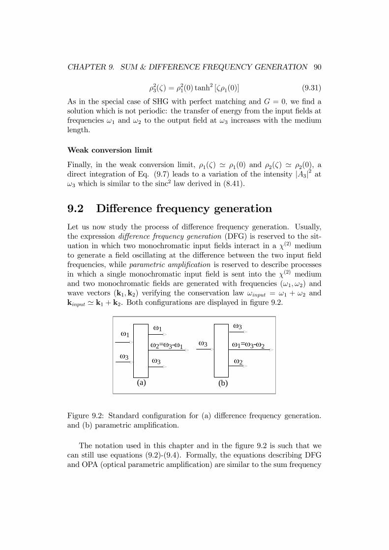
CHAPTER 9. SUM & DIFFERENCE FREQUENCY GENERATION 90
ρ23(ζ) = ρ21(0) tanh2 [ζρ1(0)] (9.31)
As in the special case of SHG with perfect matching and G = 0, we find asolution which is not periodic: the transfer of energy from the input fields atfrequencies ω1 and ω2 to the output field at ω3 increases with the mediumlength.
Weak conversion limit
Finally, in the weak conversion limit, ρ1(ζ) ' ρ1(0) and ρ2(ζ) ' ρ2(0), adirect integration of Eq. (9.7) leads to a variation of the intensity |A3|2 atω3 which is similar to the sinc2 law derived in (8.41).
9.2 Difference frequency generationLet us now study the process of difference frequency generation. Usually,the expression difference frequency generation (DFG) is reserved to the sit-uation in which two monochromatic input fields interact in a χ(2) mediumto generate a field oscillating at the difference between the two input fieldfrequencies, while parametric amplification is reserved to describe processesin which a single monochromatic input field is sent into the χ(2) mediumand two monochromatic fields are generated with frequencies (ω1, ω2) andwave vectors (k1,k2) verifying the conservation law ωinput = ω1 + ω2 andkinput ' k1 + k2. Both configurations are displayed in figure 9.2.
ω1
ω3
ω1 ω3
ω2
ω1=ω3-ω2ω2=ω3-ω1
ω3
(a) (b)
ω3
Figure 9.2: Standard configuration for (a) difference frequency generation.and (b) parametric amplification.
The notation used in this chapter and in the figure 9.2 is such that wecan still use equations (9.2)-(9.4). Formally, the equations describing DFGand OPA (optical parametric amplification) are similar to the sum frequency

CHAPTER 9. SUM & DIFFERENCE FREQUENCY GENERATION 91
generation equations, the obvious difference being in the initial condition.This is completely true for propagation in bulk materials. However, if thenonlinear medium is placed in a resonant cavity, the resulting problem issubstantially different from its SFG counterpart. The reason is linked to thefact that intracavity SHG is a thresholdless process whereas the intracavityDFG and OPA have a lasing threshold.In this section, we focus on three-wave mixing processes with two in-
put fields and three output fields, such that the new field oscillates at thedifference between the two input field frequencies. To formulate this prob-lem, we use the equations (9.5)-(9.7) to describe free running sum frequencygeneration
dA1dz
=iω1χ
(2)
ε0cn1A∗2A3e
iz∆k (9.32)
dA2dz
=iω2χ
(2)
ε0cn2A∗1A3e
iz∆k (9.33)
dA3dz
=iω3χ
(2)
ε0cn3A1A2e
−iz∆k (9.34)
with ω1 + ω2 = ω3 and ∆k = k3 − k2 − k1. The input fields are A1 and A3.
9.2.1 Two intense input fields
If both input fields are intense and depletion by transfer of energy to the fieldA2 created at the difference frequency can be neglected in first approximation,the process is described in first approximation by equation (9.33) with A1and A3 constant:
dA1dz
= 0,dA3dz
= 0, (9.35)
dA2dz
=iω2χ
(2)
ε0cn2A∗1A3e
iz∆k (9.36)
Integration over z leads to
A2(z) =ω2χ
(2)
ε0cn2A∗1A3
eiz∆k − 1∆k
(9.37)
and therefore
|A2(L)|2 =
µLω2χ
(2)
ε0cn2
¶2|A3|2 |A1|2 sinc2(L∆k/2)
=£max |A2(L)|2
¤sinc2(L∆k/2) (9.38)

CHAPTER 9. SUM & DIFFERENCE FREQUENCY GENERATION 92
This result shows a rather general property of DFG: the conversion efficiencyincreases with the frequency of the generated field. Thus conversion in theinfrared is less favorable than conversion in the visible. Another point whichis made clear by this result is the trade-off between crystal length and phase-matching. One way to increase field conversion is to use a longer crystalsince |A2(L)|2 increases with the square of the crystal length L. However,the product L∆k must also remain close to 0, which means that the longerthe crystal, the smaller ∆k must be. In practical devices, it is the phasematching condition which limits the crystal length.
9.2.2 One intense input field
More often, only one input field is intense and can be treated as a constant.The second input field serves as a ”catalyst” to induce the required frequencyω2. Let ω3 be the frequency of the intense field and ω1 the frequency of theweak input field. This situation is described by the set of coupled linearequations
dA1dz
=iω1χ
(2)
ε0cn1A∗2A3e
iz∆k (9.39)
dA∗2dz
= −iω2χ(2)
ε0cn2A1A
∗3e−iz∆k (9.40)
with A3 constant. Defining Ap = Apeiz∆k/2 leads to
dA1dz
= −i∆k
2A1 + iK1A∗2A3 (9.41)
dA∗2dz
= i∆k
2A∗2 − iK2A1A∗3 (9.42)
with
Kp =ωpχ
(2)
ε0cnp(9.43)
A simple way to solve equations (9.41)-(9.42) is to derive each of them withrespect to z :
d2Ap
dz2−K2Ap = 0 (9.44)
for p = 1, 2 and
K =
qK1K2 |A3|2 − (∆k/2)2 (9.45)
We see clearly that if K is real, K2 > 0 and the fundamental solutions of Eq.(9.44) are the functions exp (±Kz), leading to the possibility of amplification

CHAPTER 9. SUM & DIFFERENCE FREQUENCY GENERATION 93
since exp (Kz) is unbounded. IfK is imaginary, K2 < 0 and the fundamentalsolutions of Eq. (9.44) are the bounded periodic functions exp (±i |K| z)which cannot lead to anmplification.In the limit of intense pump field A3 which is defined more precisely by
the inequality K1K2 |A3|2 À (∆k/2)2 , the parameter K is real and can beinterpreted as a gain per unit length. Therefore the solutions are of the formA1(z) = a1 exp (Kz)+a2 exp (−Kz) andA2(z) = b1 exp (Kz)+b2 exp (−Kz) .The boundary conditions for DFG are A1(0) = A1 and A2(0) = 0, whichimply from (9.41)-(9.42) dA1/dz|z=0 = −i(∆k/2)A1 and dA2/dz|z=0 =−iK2A
∗3A1. Hence the solution of equations (9.41)-(9.42) is
A1(z) =A12
∙µ1− i
∆k
2K
¶eKz +
µ1 + i
∆k
2K
¶e−Kz
¸= A1
∙cosh(Kz)− i
∆k
2Ksinh(Kz)
¸(9.46)
A2(z) =iK2A
∗3A1
Ksinh(Kz) (9.47)
In terms of field intensities, we have
|A1(z)|2 = |A1|2"cosh2 (Kz) +
µ∆k
2K
¶2sinh2 (Kz)
#(9.48)
|A2(z)|2 =
µK2
K
¶2|A3|2 |A1|2 sinh2 (Kz) (9.49)
In the large z limit, that is for Kz À 1, we have the result
|A1(z)|2|A1(0)|2
=
"1 +
µ∆k
2K
¶2#e2Kz
4(9.50)
|A2(z)|2 =
µK2
K
¶2|A3|2 |A1|2 e
2Kz
4(9.51)
so that 2K is a fair measure of the intensity gain. Note that in the limitKz À 1, both fields A1(z) and A2(z) grow exponentially and at the samerate. For LiNbO4 we have χ(2)/ε0 = 2.7× 10⁻⁸esu and n1 ' n2 = 2.23 at λ1' λ2 = 1.06×10⁻⁶ m. Hence for our usual choice of the strong field |A3| = 102esu, the maximum gain (i.e., for exact phase matching) is K = 1.14 cm−1
which is quite poor.It is quite easy to assess the influence of phase matching in the case of an
intense and a weak input fields. If (∆k)2 > 4K1K2 |A3|2 , we define the realcharacteristic wave number
kc =£(∆k/2)2 −K1K2 |A3|2
¤−1/2(9.52)
CHAPTER 9. SUM & DIFFERENCE FREQUENCY GENERATION 94
in terms of which the solution (9.48) and (9.49) becomes
A1(z) = A1
∙cos (kcz)− i∆k
2kcsin (kcz)
¸(9.53)
A2(z) =K2
kcA∗3A1 sin (kcz) (9.54)
In these expressions, amplification is absent and replaced by a periodic andbounded variation of the fields as a function of the propagation distance.

Chapter 10
Optical parametric oscillator
10.1 FormulationWe have seen in the previous chapter that the yield of parametric conversionis fairly small in free space. Still, it is worth trying to improve the operatingconditions because this process is potentially a versatile source of tunableradiation in the infrared. Therefore much development has taken place toimprove the situation and today the optical parametric oscillator (OPO) isthe most widely tunable laser source used in the IR.The typical setup consists of a resonant cavity pumped by the field E3.
The χ(2) medium is in the cavity and generates the two fields E1 and E2whose frequencies add up to the frequency of the input field. We assume thatthe fields interact in a resonant cavity so that the basic modes are eitherrunning waves up =
p1/Leikpz or standing waves up =
p2/L sin (kpz). The
main assumption is that each of the three fields can be associated with one— and only one — cavity mode. The basic evolution equations (8.2) derivedin Chapter 8 become
u1dA1dt
=iω1χ
(2)
ε0n21u∗2u3A
∗2A3 − γ1u1A1 (10.1)
u2dA2dt
=iω2χ
(2)
ε0n22u∗1u3A
∗1A3 − γ2u2A2 (10.2)
u3dA3dt
=iω3χ
(2)
ε0n23u1u2A1A2 − γ3u3 (A3 − A) (10.3)
andR L0u∗puqdz = δpq. For running waves, these equations could also be de-
rived from Eqs. (9.2)-(9.4), apart from the damping and pumping termswhich are anyway added phenomenologically. We have added to each equa-tion a damping term −γpupAp to account for the cavity losses suffered by
95

CHAPTER 10. OPTICAL PARAMETRIC OSCILLATOR 96
each field. In addition, the equation for A3 contains a source term to accountfor the external pumping: in the absence of a nonlinear medium, the cavityfield at ω3 becomes in the long time limit A3 = A. These equations alreadycontain a simplifying assumption since there is no trace of the optical fre-quency: the assumption is that the driving field frequency ωe and the cavityfield frequency ω3 are sufficiently close that their difference can be neglected.We multiply the equation for Ap by u∗p and integrate over the cavity lengthto obtain
dA1dt
=iω1χ
(2)
ε0n21fA∗2A3 − γ1A1 (10.4)
dA2dt
=iω2χ
(2)
ε0n22fA∗1A3 − γ2A2 (10.5)
dA3dt
=iω3χ
(2)
ε0n23f ∗A1A2 − γ3 (A3 −A) (10.6)
where
f =
Z L
0
u∗1u∗2u3dz ≡ ϕeiφ (10.7)
10.2 Threshold conditionLet us first perform a change of variables. Defining
φp =ωp
γpn2p
χ(2)
ε0ϕ (10.8)
we introduce the change of variables
A1 = − ieiφE1pφ2φ3
, A2 =E2pφ1φ3
(10.9)
A3 = − E3pφ1φ2
, A = − Epφ1φ2
(10.10)
which leads to the evolution equations
dE1dt
= γ1 (−E1 + E∗2E3) (10.11)
dE2dt
= γ2 (−E2 + E∗1E3) (10.12)
dE3dt
= γ3 (−E3 − E1E2 + E) (10.13)
CHAPTER 10. OPTICAL PARAMETRIC OSCILLATOR 97
This result simply means that once the right scaling of the fields is introduced,the intrinsic nonlinear dynamics of the optical system is the same for anycavity provided the assumption that each lasing mode is a cavity eigenmodeis correct. What changes is the expression of the threshold at which the newfields appear.In steady state, these equations lead toE = E3
¡1 + |E1|2
¢= E3
¡1 + |E2|2
¢.
Therefore|E1|2 = |E2|2 (10.14)
and E3 is real since E is real. There are two steady state solutions to theseequations: the one-field solution
E1 = E2 = 0, E3 = E (10.15)
and the three-field solution E1 = E∗2E3 and E2 = E∗1E3 which implies E1 =E∗2E3 = E∗2E
−13 so that
|E1|2 = |E2|2 = E − 1, E3 = 1 (10.16)
The important fact to notice is the occurrence of a threshold E = Eth with
Eth = 1 (10.17)
which means |Ath|2 = (φ1φ2)−1 for the driving field and such that:• below threshold, there is no intracavity parametric process and thedriving field is simply reduced linearly by the finite reflectivity of themirrors;
• above threshold, the field amplitude at the driving frequency ω3 re-mains constant while two fields are generated by parametric amplifica-tion and grow with the driving field amplitude.
This is completely different from the thresholdless operation of intracavitySHG.
10.3 Degenerate OPOA particular configuration can be realized in which ω1 = ω2 = ω3/2. In thiscase, the problem is referred to as the degenerate optical parametric oscillator(DOPO) and it is described by the two coupled equations
dE1dt
= γ1 (−E1 + E∗1E3) (10.18)
dE3dt
= γ3¡−E3 − E2
1 + E¢
(10.19)

CHAPTER 10. OPTICAL PARAMETRIC OSCILLATOR 98
E0.0 0.5 1.0 1.5 2.0 2.5 3.0
0.0
0.5
1.0
1.5
2.0
|E3|2|E1|2
Figure 10.1: Steady state solutions of Eqs. (10.11)-(10.13).
These equations are very similar to Eqs. (8.53)-(8.54) of ISHG studied inchapter 7, except for the driving field: in ISHG, the driving field oscillatesat ω1 (in the notations of this chapter) and generates the field at ω3 = 2ω1while in the DOPO it is the driving field at ω3 that generates the field atω1 = ω3/2. This model can easily be generalized to include both drivingfields and produces an interesting phase diagram with a tricritical point.
∆1∆3>1
0 2 4 6 8 10 12 14 16 18 20
E2
0
1
2
3
4
5
|E1|2 ∆1∆3<1
Figure 10.2: Intensity |E1|2 as a function of the driving field intensity E2 for∆1 = 1, ∆3 = 1/2 and 2 in the case of a DOPO.
Let us use the simplified model of the DOPO to assess the influence ofdetuning. If the driving field is not oscillating exactly at a resonance frequencyof the cavity, we have to generalize equations (10.18) and (10.19) as follows
dE1dt
= γ1 [− (1 + i∆1)E1 + E∗1E3] (10.20)
dE3dt
= γ3£− (1 + i∆3)E3 − E2
1 + E¤
(10.21)

CHAPTER 10. OPTICAL PARAMETRIC OSCILLATOR 99
where∆1 = (ω1 − ωe/2) /γ1, ∆3 = (ω3 − ωe) /γ3 (10.22)
The frequency of the driving field is ωe while ω3 and ω1 are the cavity fre-quencies closest to ωe and ωe/2, respectively. Again, there are two possiblesteady state solutions, namely the one-field solution
E1 = 0, |E3|2 = E2
1 +∆23
(10.23)
and the two-field solutions
|E3|2 = 1 +∆21 (10.24)
0 = |E1|4 + 2 |E1|2 (1−∆1∆3)− E2 +¡1 +∆2
1
¢ ¡1 +∆2
3
¢(10.25)
The solutions of (10.25) are
|E1|2 = ∆1∆3 − 1±qE2 − (∆1 +∆3)
2 (10.26)
The threshold which separates the one-field and two-field solutions is
Eth =q(1 +∆2
1) (1 +∆23) = |∆1 +∆3| (10.27)
1 = ∆1∆3 (10.28)
We notice first that the detuning increases the threshold field, which meansthat it acts as an additional loss.
∆1
∆3
B
B
P
P
S
S
Figure 10.3: Stability boundaries for the detuned DOPO. The finite intensitysteady state solution is stable in domain S, bistable in domain B, and un-stable via a Hopf bifurcation in domain P . The boundary between S and Bis ∆1∆3 = 1. The boundary between S and P is ∆3 (γ∆3 + 2∆1) = −γ − 2.

CHAPTER 10. OPTICAL PARAMETRIC OSCILLATOR 100
This is only a quantitative modification. Much more important is thequalitative change induced by the detunings on the nature and stability ofthe solutions above threshold:
• If E > Eth, the quadratic equation (10.25) for |E1|2 has one real root if∆1∆3 < 1 and two real roots if ∆1∆3 > 1. Thus if both detunings havethe same sign and their product is larger than unity, there is a domainof bistability. Figure 10.2 displays the two types of steady solutions.
• A linear stability analysis shows that in the monostable regime (∆1∆3 <1), there can be a Hopf or selfpulsing instability of the steady state ata finite distance from the threshold. Out of this selfpulsing instability,a branch of periodic solution emerges, whose stability is subjected tofurther constraints on the detunings. The existence condition for theHopf bifurcation is
∆3 (γ∆3 + 2∆1) < − (γ + 2) (10.29)
and the field intensity at the Hopf bifurcation is
|E1,H |2 = −γ2 (1 +∆2
3)£γ2∆2
3 + (γ + 2)2¤
2 (γ + 1)2 (γ∆23 + 2∆3∆1 + γ + 2)
(10.30)
where γ = γ3/γ1 . At that point, the two fields begin to oscillate withthe frequency
Ω2H = γ21
µ2 |E1,H |2 + γ2
1 +∆23
1 + γ
¶(10.31)
This discussion is summarized in figure 10.3 which shows how the inclu-sion of simple physical parameters may lead to a wealth of new featuresin the output fields.

CHAPTER 10. OPTICAL PARAMETRIC OSCILLATOR 101
(d)
(a) (b)
02468
0 10 20 30 40 500
2
4
6
0 10 20 30 40 50
02468
10
0 10 20 30 40 50
(c)
0
40
80
120
0 10 20 30 40 50
Figure 10.4: Intensity |E1|2 of the subharmonic field as a function of thescaled time τ = γ1t obtained by numerical simulation of the DOPO equations(10.20)-(10.21) for γ = 1,∆1 = 1 and∆3 = −3. (a) E = 6: period-1 solution;(b) E = 6.5: period-2 solution ; (c) E = 6.8: period-4 solution; (d) E = 20:chaotic solution.
In figure 10.4 we display periodic and chaotic solutions of the DOPOequations (10.20)-(10.21).
10.4 Ring and Fabry-Perot cavities
Using the ring cavity running wave eigenfunctions up =p1/L exp(ikpz) leads
tof =
1√LeiL∆k/2sinc (L∆k/2) (10.32)
The relation |Ath|2 = (φ1φ2)−1 ∼ [sinc (L∆k/2)]−2 indicates that a good
control of the phase matching is essential to build a ring cavity device whichhas a threshold power as low as possible.With standing wave as cavity modes up(z) =
p2/L sin (kpz), the function
f is
f =
µ2
L
¶3/21
(2i)3
Z L
0
¡eik1z − e−ik1z
¢ ¡eik2z − e−ik2z
¢ ¡eik3z − e−ik3z
¢dz
'µ2
L
¶3/21
(2i)3
Z L
0
¡eiz∆k − e−iz∆k
¢dz
' −∆k
2
rL
2sinc2 (L∆k/2) (10.33)

CHAPTER 10. OPTICAL PARAMETRIC OSCILLATOR 102
In deriving this result, we have neglected terms oscillating fast in space,typically with wave numbers k1 ± k2 ± k3 6= ∆k, compared with the twoterms oscillating at ∆k. This configuration is known as triply resonant sinceall three modes are close to a cavity eigenmode.For the ring laser we have
|Ath|2 =µ
ε0χ(2)
¶2n21γ1ω1
n22γ2ω2
L
sinc2 (L∆k/2)(10.34)
while for the Fabry-Perot we have
|Ath|2 = 2
sin2 (L∆k/2)
(µε0χ(2)
¶2 n21γ1ω1
n22γ2ω2
L
sinc2 (L∆k/2)
)(10.35)
Thus the Fabry-Perot cavity is even more sensitive to the phase matchingcondition than the ring cavity.Let us stress that for the two OPO cavity configurations which have been
analyzed in this chapter, it was assumed that all three modes are resonants.This configuration is called the triply resonant configuration. Similarly, therecan be doubly and singly resonant settings in which only two fields or onefield, respectively, are resonant with the cavity. The non-resonant fieldssimply propagate through the χ(2) medium but do not feel the presence ofthe cavity. The description of these configurations is vastly more difficult thanthe triply resonant cavity unless the non-resonant fields are so intense thatthey can be assumed to remain constant, in which case the problem is trivialsince it reduces to a single or a pair of linear differential equations. Thedifficulty of the general situation is that the resonant fields certainly varyin time and the non-resonant fields certainly vary in space. Therefore theχ(2) coupling leads to a space-time variation for all fields. Only approximatemodels have been used in analyzing these situations.
10.5 References1. χ(2) second order nonlinear optics: from fundamentals to applications,C. Fabre and J.-P. Pocholle eds., Quantum & Semiclass. Optics 9(1997) 131-295.

Part IV
Quantum interference
103


Chapter 11
Coherence and atomicinterference
11.1 Atomic interferenceThe simplest situation in which atomic interference occurs is the interactionof a three-level medium with a bichromatic field. Let the field be given by
Etot = Ea cos(ωat) + Eb cos(ωbt) (11.1)
The three atomic wave functions are ϕj and the corresponding energies are~ωj. The interaction Hamiltonian is−erEtot. This electric field interacts witha three-level medium as shown in Fig. 11.1. This configuration is usually
Ea,ωaEb,ωb
3, ω3, ϕ3
2, ω2, ϕ2
1, ω1, ϕ1
Figure 11.1: Configuration and notations for the three-level medium inter-acting with two monochromatic fields.
referred to as the Λ configuration. The other two possibilities are:
104

CHAPTER 11. COHERENCE AND ATOMIC INTERFERENCE 105
• The V configuration where the monochromatic fields connect levels 1to 2 and levels 1 to 3;
• The ladder configurations where the monochromatic fields connect lev-els 1 to 2 and levels 2 to 3.
The main point is that in the Λ configuration, an atom in state 3 maydecay either through the channel 3 − 1 or through the channel 3 − 2. Inthe case of two levels, the probability that the atom decays from the upperstate 3 to the lower state 1 is of the form P (3 → 1) = |C31|2 where thecomplex coefficient C31 is related to the expansion of the total wave functionon the basis of the atomic wave functions. When two decay channels areavailable, the probability is of the form P (3) = |C31 + C32|2 which is the sumof two complex functions, each one associated with one of the decay chan-nels. Hence the total transition probability is not be the sum of the partialtransition probabilities: P (3) 6= P (3→ 1)+P (3→ 2): there are interferenceterms which need not be positive. We shall see that these interference termsmay compensate, partially or completely, the partial transition probabilities,therefore reducing the decay probability from level 3.As a practical example, let us consider a three-level system interacting
with the bichromatic field (11.1). We still have to specify the selection rules.Let them be given by
hj |erEa| 3i = µEδj1 hj |erEb| 3i = µEδj2 (11.2)
with all other matrix elements being zero. This corresponds to the interactionscheme of Fig. 11.1. The matrix elements are defined as usual by hj |O| ki =RVϕ∗j(r)O(r)ϕk(r)dr for an operator O ≡ O(r). To simplify the algebra of
this example, we have assumed that the matrix elements are identical whenthey do not vanish. This simplification is without influence on the qualitativephysical results described in this section.Let us now assume that a superposition state Φ(r, t) = C1(t)ϕ1(r) +
C2(t)ϕ2(r) can be created. Then the probability of transition from state 3to that superposition state is given by
W1 =¯C1ϕ1e
−iω1t + C2ϕ2e−iω2t |−erEtot| e−iω3tϕ3
®¯2=
|µE|24
¯C1e
i(ω31−ωa)t + C2ei(ω32−ωb)t¯2 (11.3)
where ωjk ≡ ωj − ωk. The case ω31 − ωa = ω32 − ωb is of special interest.If this condition is verified, that is, if the detuning between the field Ea andthe atomic energy difference ω31 equals the detuning between the field Eb

CHAPTER 11. COHERENCE AND ATOMIC INTERFERENCE 106
and the atomic difference ω32, then the transition probability W1 becomesconstant in time
W1 =1
4|µE(C1 + C2)|2 (11.4)
To appreciate more fully this result, let us consider another possible set ofselection rules. Let us assume that each field Ej couples equally the upperlevel 3 to the two lower states
ϕj |erEa|ϕ3®=ϕj |erEb|ϕ3
®= µE, j = 1, 2 (11.5)
This could be the case if ω2 − ω1 ≪ ω3. In this case, using again thecondition of equal detuning ω31−ωa = ω32−ωb, the probability of transitionbetween the upper state and the state Φ becomes
W2 =|µE|24
¯C1(1 + eiω12t) + C2(1 + e−iω12t)
¯2(11.6)
There is no way in which this function can become time-independent: it isand remains a periodic function of time with period T = 2π/ω12. This showshow critical the selection rules become in the three-level case.Let us consider again the first case which yields the transition probability
W1. An interesting situation occurs if the superposition state is Φ− = C1(ϕ1−ϕ2), i.e., C1 = −C2. In this case W1 = 0 as a result of maximum destructiveinterference. Indeed, the vanishing of W1 results from the relations |C1|2 =|C2|2 = −C1C∗2 = −C∗1C2. Physically, this means that an atom which isinitially in the upper state will be unable to decay in the state Φ− via adipole-mediated transition. Conversely, an atom which is initially in the stateΦ− will remain in that state. Such states are called trap states1.There still remains to produce the superposition stateΦ(r, t) = C1(t)ϕ1(r)+
C2(t)ϕ2(r). In quantum mechanics, the states Φ± = 1√2(ϕ1 ± ϕ2) appear in
the study of the eigenstates of a two-level atom interacting resonantly witha single mode of the electromagnetic field. In that context, there is a unitaryoperator which maps the unperturbed basis ϕ1, ϕ2 into the eigenstates ofthe total Hamiltonian Φ−,Φ+. These two states have a different energydue to the Stark splitting. It is easily verified that the state Φ+ has a nonzerotransition probability with the upper state 3, as should be. As a result, itappears that what matters is the amount of atomic population in the upperlevel and in the combination state Φ+. The surprise is that situations can be
1O. Kocharovskaya, Phys. Rep. 219, 175 (1992); P. Mandel, Contemp. Physics 34(1993) 235; E. Arimondo, in Progress in Optics XXXV, edited by E. Wolf (Elsevier,Amsterdam, 1996) 257.

CHAPTER 11. COHERENCE AND ATOMIC INTERFERENCE 107
conceived (and realized experimentally2) where there is an inversion of pop-ulation between the upper state and Φ+, and therefore gain or even lasing,while there is no population inversion between the upper state and the lowerstates ϕ1 and ϕ2. This phenomenon is referred to as gain without inversionor lasing without inversion.
11.2 Semiclassical formulationIn this section, we formulate more rigorously the scheme which was describedin Section 11.1. We can use the semiclassical formulation developed in Chap-ter 1 since it is based on a quantum description of matter and a classicaldescription of the electromagnetic fields. This is sufficient to include atomicinterference effects.The procedure is similar to that used for the two-level medium. The
electric field and atomic polarization are decomposed as follows
Etot =1
2
£Eae
i(kax−ωat) + Ebei(kbx−ωbt) + c.c.
¤(11.7)
Ptot = N£Pae
i(kax−ωat) + Pbei(kbx−ωbt) + c.c.
¤(11.8)
Let us consider the atomic scheme of Fig. 11.1. It is described by the wavefunction Ψ with the properties
i~∂Ψ
∂t= HΨ = (H0 + V )Ψ (11.9)
Ψ = a1ϕ1 + a2ϕ2 + a3ϕ3 (11.10)
1 = |a1|2 + |a2|2 + |a3|2 (11.11)
H0ϕk = ~ωkϕk, V = −erEtot (11.12)
In the dipole approximation, the matrix elements of the perturbation are
V12 = 0, V13 = −µ13Etot, V23 = −µ23Etot (11.13)
With these expressions, we can derive the evolution equations for the coeffi-cients ak in Ψ
i~∂ta1 = ~ω1a1 − µ13a3Etot (11.14)
i~∂ta2 = ~ω2a2 − µ23a3Etot (11.15)
i~∂ta3 = ~ω3a3 − µ32a2Etot − µ31a1Etot (11.16)2A. Nottelmann, C. Peters, and W. Lange, Phys. Rev. Lett. 70, 1783 (1993); E.S. Fry,
Xingfu Li, D. Nikonov, G. G. Padmabandu, M.O. Scully, A.V. Smith, F.K. Tittel, ChingWang, S.R. Wilkinson, and Shi—Yao Zhu, Phys. Rev. Lett. 70, 3235 (1993); W. E. vander Veer, R. J. J. van Diest, A. Dönszelmann, and H. B. van Linden van den Heuvell,Phys. Rev. Lett. 70, 3243 (1993).

CHAPTER 11. COHERENCE AND ATOMIC INTERFERENCE 108
The next step is the derivation of evolution equations for the density matrix.Using the definition ρkl = aka
∗l and Eqs. (11.14)-(11.16), it is easy to derive
the evolution equations
i~∂tρ31 = ~ (ω3 − ω1) ρ31 + µ31 (ρ33 − ρ11)Etot − µ32ρ21Etot (11.17)
i~∂tρ32 = ~ (ω3 − ω2) ρ32 + µ32 (ρ33 − ρ22)Etot − µ31ρ12Etot (11.18)
i~∂tρ21 = ~ (ω2 − ω1) ρ21 + ρ23µ31Etot − µ23ρ31Etot (11.19)
At this point, we use the fact that ωa ' ω31 and ωb ' ω32 to introduce slowlyvarying envelopes σpq
ρ31 = σ31ei(kax−ωat), ρ32 = σ32e
i(kbx−ωbt) (11.20)
For the low frequency coherence ρ21, the slowly varying envelope σ21 is
ρ21 = σ21ei(ωb−ωa)t−i(kb−ka)x (11.21)
Using the rotating wave approximation, which amounts to neglect fast oscil-lating terms, these definitions lead to the evolution equations
i~∂tσ31 = ~ (ω31 − ωa)σ31 + n31µ312Ea − σ21
µ322Eb (11.22)
i~∂tσ32 = ~ (ω32 − ωb) σ32 + n32µ322Eb − σ12
µ312Ea (11.23)
i~∂tσ21 = ~ (ω21 − ωa + ωb) σ21 + σ23µ312Ea − σ31
µ232E∗b (11.24)
where we have used the notation npq = ρpp−ρqq for the population differences.As a final step, we introduce phenomenologically the damping rates for thethree coherence functions. This leads to the set of equations
∂tσ31 = − (γ31 + iδa) σ31 − in31µ312~
Ea + iσ21µ322~
Eb (11.25)
∂tσ32 = − (γ32 + iδb)σ32 − in32µ322~
Eb + iσ12µ312~
Ea (11.26)
∂tσ21 = − [γ21 + i (δa − δb)]σ21 − iσ23µ312~
Ea + iσ31µ232~
E∗b (11.27)
where δa = ω31−ωa and δb = ω32−ωb. An essential feature is that althoughthe electromagnetic field couples only level 3 to levels 1 and 2, there appearsa low frequency coherence σ21 even though the 2 ⇔ 1 transition has beenassumed to be forbidden.The closure of the semiclassical theory implies the relations between the
components Pj of the polarization and the density matrix are
Pa = µ13ρ31ei(ωat−kax) ≡ µ13σ31, Pb = µ23ρ32e
i(ωbt−kbx) ≡ µ23σ32(11.28)

CHAPTER 11. COHERENCE AND ATOMIC INTERFERENCE 109
Therefore, in the slowly varying envelope approximation, the two field equa-tions are ¡
∂x + v−1a ∂t + κa¢Ea = (iNµ13ωa/vaε
0a)σ31 (11.29)¡
∂x + v−1b ∂t + κb¢Eb = (iNµ23ωb/vbε
0b)σ32 (11.30)
where va,b = c/na,b and na,b is the refractive index of the passive medium atfrequency ωa,b.To be complete, we should write the evolution equations for the popu-
lations ρjj. However, these equations are not necessary for the remaining ofthis chapter.
11.3 Electromagnetically induced transparency(EIT)
In this section, we consider the following problem: assuming Eb to be astrong field, how does it affect the optical properties of the 3− 1 transition?To answer this question, we consider Eqs. (11.25) - (11.27) for the inducedatomic coherence. In steady state, we have
σ31 = −iµ312~
Ean31γ31 + iδa
+iµ322~
Ebσ21γ31 + iδa
(11.31)
σ32 = −iµ322~
Ebn32γ32 + iδb
+iµ312~
Eaσ12γ32 + iδb
(11.32)
σ21 =i (µ23Eb)
∗ σ312~ [γ21 + i (δa − δb)]
− iµ31Eaσ232~ [γ21 + i (δa − δb)]
(11.33)
At this point, we introduce four simplifications:
1. We assume that the populations ρkk do not change much under theinfluence of the applied fields: ρkk ' n
(0)k . It is not easy to justify
this simplification, except for the fact that it is validated by the fullcalculation made without that approximation. It is in fact a versionof the linear approximation introduced for the two-level model in Sec.2.1 via Eq. (2.3).
2. Without external fields we have n(0)3 = n(0)2 e−β~ω32 and n(0)2 = n
(0)1 e−β~ω21.
Hence n(0)1 À n(0)2 À n
(0)3 . Therefore, we introduce the simplification
n(0)1 = 1 and n
(0)3 = n
(0)2 = 0 which is surely valid at room temperature
in the absence of driving field.

CHAPTER 11. COHERENCE AND ATOMIC INTERFERENCE 110
3. Since the field Eb is an intense field which drives the atomic systemand Ea is a weak field, we only retain in the solutions of Eqs. (11.31)-(11.33) terms linear in the weak field Ea but make no simplificationwith respect to the strong driving field.
4. The field Eb is resonant with the atomic transition it drives: δb = 0.
With these simplifications, the solutions of equations (11.31)-(11.33) areeasily found to be
σ31 =i2~µ31Ea (γ12 + iδa)
4~2 (γ21 + iδa) (γ31 + iδa) + |µ32Eb|2(11.34)
σ21 = − (µ31Ea)∗ µ32Eb
4~2 (γ21 − iδa) (γ31 − iδa) + |µ32Eb|2(11.35)
σ32 =iµ13Ea
2~γ32σ21 (11.36)
Thus the susceptibility at the transition 3 − 1 as influenced by the intensefield Eb driving the 3− 2 transition is
χ =Pa
Ea=
µ13σ31Ea
=i2~ |µ31|2 (γ12 + iδa)
4~2 (γ21 + iδa) (γ31 + iδa) + |µ32Eb|2
= i|µ31|22~γ31
γ + iδ
(γ + iδ) (1 + iδ) + |µ32Eb/2~γ31|2(11.37)
with the dimensionless parameters γ = γ21/γ31 and δ = δa/γ31 = (ω31 − ωa) /γ31.The real and imaginary parts of the susceptibility (11.37) are
χ0 =|µ31|22~γ31
δ¡γ2 + δ2 − Ω2
¢¡γ − δ2 + Ω2
¢2+ δ2 (γ + 1)2
(11.38)
χ00 =|µ31|22~γ31
γ2 + δ2 + γΩ2¡γ − δ2 + Ω2
¢2+ δ2 (γ + 1)2
(11.39)
with the dimensionless field amplitude defined by Ω = |µ32Eb| /2~γ31.The way in which Eb influences the 3 − 1 transition is displayed in Fig.
11.2. We see that for a weak driving field (Ω¿ 1), the susceptibility hasqualitatively the same shape as for the two-level medium (see Fig. 2.1).This means that the system is transparent (χ0 = 0) where the absorptionis maximum (χ00 = 1). As the driving field increases, a dip appears in χ00 atthe point of transparency and finally it practically reaches zero. At δ = 0,

CHAPTER 11. COHERENCE AND ATOMIC INTERFERENCE 111
Ω = 0.1Ω = 0.005
χ''
-0.5
0.0
0.5
1.0
-4 -2 0 2 4-0.5
0.0
0.5
1.0
-2 -1 0 1 2
-0.5
0.0
0.5
1.0
-4 -2 0 2 4-0.5
0.0
0.5
1.0
-4 -2 0 2 4
Ω = 2Ω = 1
χ'
χ''χ''
χ''χ'
χ' χ'
Figure 11.2: Real and imaginary parts of the susceptibility at the 3-1 tran-sition as a function of δ = (ω31 − ωa) /γ31, the normalized detuning betweenthe atomic energy difference ω31 and the probe field frequency ωa. Unitsof the susceptibility are |µ31|2 / (2~γ31). Four different values of the fieldΩ = |µ32Eb| / (2~γ31) driving the 3-2 transition are chosen. The ratio γ21/γ31is 10−2.
χ00 = γ/ (γ + Ω2) → γ/Ω2 in the limit Ω À γ. Thus the absorption coeffi-cient at the 3− 1 transition becomes close to zero as the driving field at the3− 2 transition increases. In this way, atomic interference leads to a reduc-tion of the absorption coefficient at δ = 0. The deformations of χ0 and χ00
under the influence of Ω preserve the property that zeroes of χ0 correspondto extrema of χ00. The phenomenon of (near) cancellation of the absorptionat transparency is known as electromagnetically induced transparency (EIT).It was first predicted theoretically3. The first experimental observation wasreported by the same group the next year4. They used a 10 cm cell con-taining a gas of neutral Sr
¡5× 10¹⁵ atoms/cm3¢. The transition which was
probed was the 5s5p1P1 − 4d5d1D2 transition at 337.1nm. In the absence ofanother field, the cell absorption at that frequency was e−20. In the presenceof a strong field driving the 4d5p1D2 − 4d5d1D2 transition at 570.3nm, theabsorption of the cell was reduced to e−1.The obvious advantage of this scheme over the saturation bleaching is that
in the latter case the medium is made transparent by saturation and this re-quires the use of intense fields. Since there is dispersion and nonlinearity, thebeam which eventually succeeds in traversing the medium has lost significantpower and beam quality: the field distribution in the plane transverse to thepropagation direction is highly inhomogeneous. This is inacceptable for manyapplications. On the contrary, in the EIT scheme, it is an adjacent transition
3S.E. Harris, J.E. Field, and A. Imamoglu, Phys. Rev. Lett. 64 (1990) 1107.4K.J. Boller, I. Imamoglu, and S.E. Harris, Phys. Rev. Lett. 66 (1991) 2593.

CHAPTER 11. COHERENCE AND ATOMIC INTERFERENCE 112
which is strongly driven. Furthermore, the EIT scheme allows the use of adriving field at a different frequency than the probed transition. This is canbe exploited to drive at a low frequency and probe at a higher frequency.
11.4 Slow lightOne observation about EIT as displayed in Fig. 11.2 is that the slope of χ0
close to δ = 0 changes sign and can be very steep. Therefore, one shouldexpect that properties depending on that slope will manifest a markedlydifferent behavior in the case of EIT. One such property is the group velocityor the group refractive index defined by Eq. (2.47). In this case, ∂n/∂k = 0so that we are left with
vg ≡ ∂ω
∂k=
c
n+ ω ∂n∂ω
≡ c
ng(11.40)
This leads to an unexpected consequence of EIT, namely the possibilityto control the speed of light, to cancel it and even to make it negative5.Of course, this does not refer to the phase velocity but only to the groupvelocity. Still, it is the group velocity which is relevant for many applicationssince that is the velocity which affects the speed of the wave packet, i.e., thetransport of energy. Using the expression (11.38) for the real part of thesusceptibility and the definition n =
√1 + χ0, it is easy to verify that close to
the resonance (δ = 0) the refractive index n and the group refractive indexng are given by the following expansions
n = n0 + n1δ +O(δ2) = 1− |µ31|2
4~γ31Ω2 − γ2
(γ − Ω2)2δ +O(δ2) (11.41)
ng = n0g +O(δ) = 1 + |µ31|2
4~γ31ω31γ31
Ω2 − γ2
(γ − Ω2)2+O(δ) (11.42)
To avoid jumping too quickly to wrong conclusions, it should be clear thatthe expansion in powers of δ converges if and only if the coefficient of δn
is smaller than the coefficient of δn−1. Otherwise, n and ng must be usedwithout approximations. The double constraint of |n1δ| ¿ n0 and n0g À 1leads to the condition |δ| ¿ ω31/γ31, which is physically realizable.FromEqs. (11.41)-(11.42) it is seen that in the conditions of EIT for which
the expressions (11.38)-(11.39) hold for the susceptibility, the refractive index
5A review of this topic is presented in Slow, ultraslow, stored, and frozen light, A.B.Maysko, O. Kocharovskaya, Yu. Rostovtsev, G.R. Welch, A.S. Zibrov, and M.O. Scully,Adv. Atom. Mol. Opt. Phys. 46 (2001) 191-242.

CHAPTER 11. COHERENCE AND ATOMIC INTERFERENCE 113
equals unity on resonance while the group refractive index can be made verylarge in the domain |δ| ¿ ω31/γ31. Thus, we arrive at the following situationon resonance:
• In the absence of a driving field (Ω = 0), the refractive index equalsunity but the absorption is maximum: the probe field Ea suffers maxi-mum absorption, which may make the medium opaque to the radiationat the frequency ωa.
• Applying a strong driving field to excite the adjacent coherence betweenlevels 3 and 2 has the effect of modifying the optical properties of thecoherence between levels 3 and 1, resulting in a transparency of themedium at the frequency ωa since χ00(ωa) ' 0 without dispersion sincen = 1.
• When this is realized, and if the condition |δ| ¿ ω31/γ31 is verified,the group refractive index is very large, which means that the groupvelocity is very small. Light propagating in these conditions is calledslow or ultraslow light6. Group velocities of a few meters per second inthe visible range are now realized without problems in various media(gas and solid-state) at room temperature.
• If the medium is inhomogeneous, there is a further source of reductionsince in that case the group velocity is given by the complete expression(2.47)
vg ≡ ∂ω
∂k=
c− ω ∂n∂k
n+ ω ∂n∂ω
(11.43)
• Under suitable conditions, the group velocity can vanish7 and evenbecome negative. This has been achieved experimentally8. A posi-tive/negative group velocity means that the wave packet moves in the
6L.V. Hau, S. E. Harris, Z. Dutton, and C. H. Behroozi, Nature (London) 397, 594(1999); M. Kash, V. Sautenkov, A. Zibrov, L. Hollberg, G. Welch, M. Kukin, Y. Rostovsev,E. Fry, and M. Scully, Phys. Rev. Lett. 82, 5229 (1999); D. Budker, D. F. Kimball, S.M. Rochester, and V. V. Yashchuk, Phys. Rev. Lett. 83, 1767 (1999).
7M.D. Lukin, S. F.Yelin, and M. Fleischhauer, Phys. Rev. Lett. 84, 4232 (2000); A. E.Kozhekin, K. Mølmer, and E. Polzik, Phys. Rev. A 62, 033809 (2000); O. Kocharovskaya,Yu. Rostovtsev, and M. O. Scully, Phys. Rev. Lett. 86, 628 (2001).
8C. Liu, Z. Dutton,C. H. Behroozi, and L.V. Hau, Nature 409, 490 (2001); D. F.Phillips,A. Fleischhauer,A.Mair, R. L.Walsworth, and M.D. Lukin, Phys. Rev. Lett. 86,783 (2001); A. Mair, J.Hager,D. F. Phillips, R. L.Walsworth, and M. D. Lukin, Phys.Rev. A 65, 031802R (2002); A.V. Turukhin, V. S. Sudarshanam, and M. S. Shahriar,J. A. Musser, B. S. Ham, and P. R. Hemmer, Phys. Rev. Lett. 88, 023602 (2002); A.S. Zibrov, A. B. Matsko, O. Kocharovskaya, Y.V. Rostovtsev, G. R. Welch, and M. O.Scully, Phys. Rev. Lett. 88, 103601 (2002).

CHAPTER 11. COHERENCE AND ATOMIC INTERFERENCE 114
forward/backward direction. Controlling the sign of the group velocitymay have potential applications to an all-optical read/write process.