In-body Path Loss Model for Homogeneous Human

Tissues

Divya Kurup, Wout Joseph, Gunter Vermeeren, and Luc Martens

IBBT-Ghent University, Dept. of Information Technology

Gaston Crommenlaan 8 box 201, B-9050 Ghent, Belgium

Fax: +32 9 33 14899, E-mail: divya.kurup@intec.UGent.be

Abstract

A wireless body area network (WBAN) consists of a wireless network with devices placed close to,

attached on, or implanted into the human body. Wireless communication within human body experiences

loss in the form of attenuation and absorption. A path loss model is thus necessary to identify these losses in

homogeneous medium which is proposed in this paper. The model is based on 3D electromagnetic simulations

and is validated with measurements. Simulations are further extended for different relative permittivity ǫr

and conductivity σ combinations spanning a range of human tissues at 2.45 GHz, and the influence of

the dielectric properties on path loss is investigated and modeled. This model is valid for insulated dipole

antennas separated by a distance up to 8 cm. Further, path loss in homogeneous medium is also compared

with the path loss in heterogeneous tissues. The path loss model for homogeneous medium is the first in-

body model as a function of ǫr, σ, and separation between antennas and can be used to design an in-body

communication system.

Index Terms

Wireless body area networks (WBAN), Homogeneous medium, Heterogeneous medium, Path loss model,

Insulation, Dipole antenna, Simulations, Measurements

I. INTRODUCTION

A wireless body area network (WBAN) is a network, consisting of nodes that communicate wirelessly

and are located on or in the body of a person. These nodes form a network that extends over the body of

a person. Depending on the implementation, the nodes consist of sensors and actuators, placed in a star

or multihop topology [1].

Applications of WBANs include medicine, sports, military, and multimedia which utilizes the freedom

of movement provided by the WBAN. As a WBAN facilitates unconstrained movement amongst users, it

has brought a revolutionary change in patient monitoring and health care facilities. Active implants placed

within the human body lead to better and faster diagnosis thus improving the quality of life of the patient.

The PL model developed in this paper focuses on deep tissue implants such as endoscopy capsule. In

such an application the implants go deep inside the body, which we have selected up to a distance of

8 cm. A PL model will help in understanding the influence of the dielectric properties of the surrounding

tissues and the power attenuation of such implants.

Knowledge of the electromagnetic fields of active implants in the body is important for electromagnetic

compatibility (EMC) studies, for the design of antennas in dielectric media, and for assessing potential

health effects of electromagnetic radiation. The degree to which antennas can communicate with each other

in a medium, characterized using the concept of path loss, is an important aspect of EMC research.The

human body is a lossy medium, hence waves propagating from the transmitter are attenuated considerably

before they reach the receiver. A path loss (PL) model helps to design optimum communication between

nodes placed within or on the human body. To our knowledge there is very limited literature on propagation

loss within the human body. In [2], initial results of an in-body propagation model in saline water

is presented.Inaccuracies lead to large maximum deviations of 9 dB between the measurements and

simulations. [2] considers a non-insulated hertzian dipole, hence the PL model can be applied only to

very small dipole antennas. [3] provides various scenarios for channel modeling but does not provide

a model for path loss. [4] discusses a link budget for an implanted cavity slot antenna at 2.45 GHz.

However, no model for various human tissues is suggested that can be used for path loss simulation. [5]

discusses how standard antenna analysis techniques fail when antennas are in a conducting medium and

emphasizes the determination of antenna gain in a conducting medium. However, it does not mention

anything regarding path loss in the conducting medium.

The goal of this paper is to develop an empirical PL model for various homogeneous human tissues

that describes the relationships between the PL and the relative permittivity ǫr and the conductivity

σ of the human tissues, the distance between the antennas and the power attenuation. We also compare

the PL in homogeneous medium with the PL in heterogeneous medium and explain the relationship

between them. Simulations and measurements are performed at 2.457 GHz in the license free industrial,

scientific and medical (ISM) band. This frequency band is chosen as there are no licensing issues in

this band and higher frequency allows the use of a smaller antenna. First we perform measurements

and simulations in homogeneous human muscle tissue. To validate the simulations with measurement,

we use a flat phantom [6] filled with human muscle simulating liquid. After validating the simulations

with measurements in human muscle tissue, simulations are extended over a broad range of ǫr and σ

representing various homogeneous human tissues to calculate the PL. The PL thus obtained is used to

propose a PL model applicable for the various homogeneous tissues in a human body.

As it is difficult for the manufacturers to test their system on actual humans, the proposed model can

be used by them to evaluate the performance of in-body WBAN systems using well specified setups and

to carry out link budget calculations. The path loss occurring in in-body is critical and the PL model can

help to find out the maximum distance that can be covered between the Tx and the Rx within the body.

Thus this model can be used for the in-body part of the link budget.

The outline of this paper is as follows. In Section II, the simulation and measurement setups are

discussed. Section III discusses the results including the reflection coefficient and the path loss of the

insulated dipole in human muscle tissue medium. The influence of ǫr and σ on path loss, the path

loss model, and the validation of the models are presented in Section IV. Section V presents the PL in

hetereogeneous medium and finally, Section VI presents the conclusions.

II. HOMOGENEOUS HUMAN TISSUES: METHOD

A. Setup for One Type of Tissue : Human Muscle Tissue

We first investigate wave propagation at 2.457 GHz in human muscle tissue (relative permittivity

ǫr = 50.8 and conductivity σ = 2.01 S/m [7]) using measurements and simulations for insulated

dipoles. After validation of the simulations and measurements for human muscle tissue, simulations are

further extended for a broad range of homogeneous human tissues which is discussed in Section II-B.

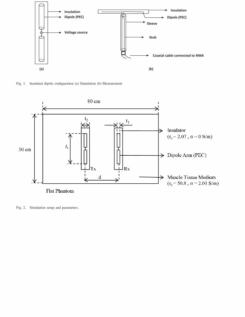
We develop two identical insulated dipoles (Fig. 1) for measurements where the dipole arms are perfect

electric conductors (PEC) surrounded with an insulation made of polytetrafluoroethylene (ǫr = 2.07 and

σ = 0 S/m). We use dipole antennas for our study as they are the best understood antennas in free

space and have a simple structure. Resonance is obtained for the insulated dipole antennas developed for

measurements at a length ℓ1 = 3.9 cm, for a frequency of 2.457 GHz. The resonance appears when the

antenna is about equal to half the wavelength in a homogeneous medium equivalent to the combination

of the insulation and the muscle tissue medium. Hence λres = 7.8 cm (where λres is the wavelength at

which resonance occurs) and we can derive the equivalent permittivity ǫr,equiv = 2.45 which is closer to

the permittivity of the insulation than to the muscle tissue. The dipole arms have a diameter t1 = 1 mm

and the diameter of the insulation is t2 = 5 mm. We use these dimensions in order to model the insulated

dipole antennas in the simulation tools. Insulated dipoles are selected instead of bare dipoles because

the insulation prevents the leakage of conducting charges from the dipole and reduces the sensitivity of

the entire distribution of current to the electrical properties of the ambient medium. This property makes

insulated dipoles valuable for WBAN purposes [8], [9].

1) Measurements: Measurements are executed using a vector network analyzer NWA (Rohde & Schwarz

ZVR) and the scattering parameters |S11|dB and |S21|dB (with respect to 50 Ω) between Tx and Rx

for the different separations are determined. The path loss is then calculated from |S21|dB as shown in

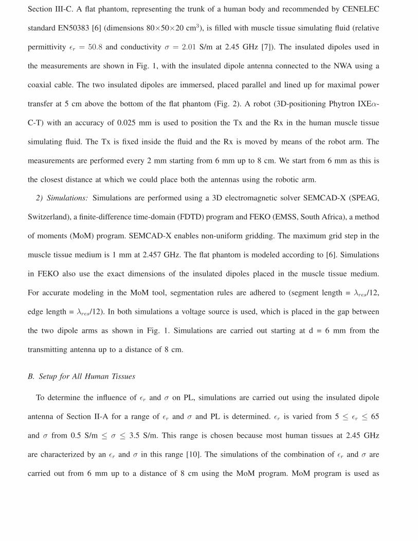
Section III-C. A flat phantom, representing the trunk of a human body and recommended by CENELEC

standard EN50383 [6] (dimensions 80×50×20 cm3), is filled with muscle tissue simulating fluid (relative

permittivity ǫr = 50.8 and conductivity σ = 2.01 S/m at 2.45 GHz [7]). The insulated dipoles used in

the measurements are shown in Fig. 1, with the insulated dipole antenna connected to the NWA using a

coaxial cable. The two insulated dipoles are immersed, placed parallel and lined up for maximal power

transfer at 5 cm above the bottom of the flat phantom (Fig. 2). A robot (3D-positioning Phytron IXEα-

C-T) with an accuracy of 0.025 mm is used to position the Tx and the Rx in the human muscle tissue

simulating fluid. The Tx is fixed inside the fluid and the Rx is moved by means of the robot arm. The

measurements are performed every 2 mm starting from 6 mm up to 8 cm. We start from 6 mm as this is

the closest distance at which we could place both the antennas using the robotic arm.

2) Simulations: Simulations are performed using a 3D electromagnetic solver SEMCAD-X (SPEAG,

Switzerland), a finite-difference time-domain (FDTD) program and FEKO (EMSS, South Africa), a method

of moments (MoM) program. SEMCAD-X enables non-uniform gridding. The maximum grid step in the

muscle tissue medium is 1 mm at 2.457 GHz. The flat phantom is modeled according to [6]. Simulations

in FEKO also use the exact dimensions of the insulated dipoles placed in the muscle tissue medium.

For accurate modeling in the MoM tool, segmentation rules are adhered to (segment length = λres/12,

edge length = λres/12). In both simulations a voltage source is used, which is placed in the gap between

the two dipole arms as shown in Fig. 1. Simulations are carried out starting at d = 6 mm from the

transmitting antenna up to a distance of 8 cm.

B. Setup for All Human Tissues

To determine the influence of ǫr and σ on PL, simulations are carried out using the insulated dipole

antenna of Section II-A for a range of ǫr and σ and PL is determined. ǫr is varied from 5 ≤ ǫr ≤ 65

and σ from 0.5 S/m ≤ σ ≤ 3.5 S/m. This range is chosen because most human tissues at 2.45 GHz

are characterized by an ǫr and σ in this range [10]. The simulations of the combination of ǫr and σ are

carried out from 6 mm up to a distance of 8 cm using the MoM program. MoM program is used as

simulations using this program are faster than the FDTD program. The setup is the same as mentioned

in the Section II-A2. In FEKO we use a current source because of the use of the finite element method

(FEM). A total of 1547 simulations were carried to obtain the return loss and PL as a function of distance

d, σ, and ǫr.

III. RESULTS : HUMAN MUSCLE TISSUE

A. Return Loss for a Single Insulated Dipole

The measured and simulated reflection losses of the insulated dipole in human muscle tissue as a

function of frequency are compared in Fig. 3. The agreement obtained between the measured and the

simulated insulated dipoles at 2.457 GHz is acceptable. The simulated and the measured dipoles are well

matched radiators in human muscle tissue. The |S11|dB for the insulated dipoles at 2.457 GHz is -13.60 dB,

-12.29 dB, and -11.25 dB for the measurements, FDTD, and MoM tool respectively. Differences in the

|S11|dB between the two simulation tools can be attributed to the inherent different modeling techniques.

B. Influence of Thickness of Insulation on the Resonance Frequency

In this section the influence of the insulation thickness t on the resonance frequency is studied. We define

t as ( t2−t12

) where t2 is the diameter of the insulation and t1 is the diameter of the dipole (PEC) (See.Fig. 2).

The influence of t from 0.1 mm up to 4.5 mm is studied. We define resonance frequency as the frequency

where the imaginary part of the input impedance is zero [11]. Fig. 4 shows that an increase in thickness

of the insulation causes the resonance frequency to increase. Hence the length of the insulated antenna

as well as the thickness of the insulation have an effect on the resonance frequency of the antenna. t

of 0.4 mm causes the antenna to resonate at a lower frequency of 1.31 GHz than that with a thickness

of 1 mm resulting in a resonance frequency of 1.86 GHz (Fig. 4). As t increases, the ǫr,equiv of the

insulation and the medium decreases and the ǫr,equiv will become closer to the value of the permittivity of

the insulator. Thus, when t increases the resonance frequency will increase which can be seen in Fig. 4.

In order to achieve a certain resonance frequency for the antenna varying the insulation thickness can

be considered as an option. Fig. 5 shows that the -10 dB bandwidth (BW) of |S11|dB as a function of

t is large enough to cover the whole of the ISM band at 2.45 GHz for our configuration which has an

insulation thickness of 4.5 mm. The insulated dipole antenna is best matched for t = 1 mm, however with

a t = 4.5 mm we have an antenna that operates in the ISM band.

C. Path Loss

PL is defined as the ratio of input power at port 1 (Pin) to power received at port 2 (Prec) in a two-

port setup. PL in terms of transmission coefficient is defined as 1/|S21|2 with respect to 50 Ω when the

generator at the Tx has an output impedance of 50 Ω and the Rx is terminated with 50 Ω. This allows

us to regard the setup as a two-port circuit for which we determine |S21|dB with reference impedances of

50 Ω at both ports:

PL|dB = (Pin/Prec) = −10 log10 |S21|2 = −|S21|dB, (1)

Fig. 6 shows the simulated and measured PL in human muscle tissue as a function of distance d for

the insulated dipole. The measured and the simulated values show excellent agreement up to 8 cm. The

deviations between the measurements and the simulations are very low: with SEMCAD-X, the maximal

and average deviation up to 8 cm are 1.7 dB and 0.8 dB, respectively, and for FEKO the maximal and

average deviation are 3.4 dB and 1.3 dB, respectively.

1) PL Model: In this section the measurement results are used to develop a PL model as a function of

distance in human muscle tissue at 2.457 GHz. The measurements and the fitted model in human muscle

tissue are shown in Fig. 6. The PL is modeled as follows :

PL|dB = (10 log10 e2) α1 d+ C1|dB for d ≤ dbp, (2)

PL|dB = (10 log10 e2) α2 d+ C2|dB for d ≥ dbp, (3)

where the parameters α1 and α2 are the attenuation constants [ 1cm

], C1|dB and C2|dB are constants,

dbp = 2.78 cm is the breakpoint where the mutual coupling between the transmitter and the receiver

ends, and d is in cm. The model consists of two regions : Region 1 and Region 2. Region 1, d ≤ dbp

is defined as the region which is very close to the Tx dipole and extends from 0 cm to 2.78 cm. Here

the Tx and the Rx are close to each other and this causes the antennas to interact with each other and

alter the impedances due to mutual coupling. In Region 2, d ≥ dbp, the mutual coupling between the Tx

and the Rx disappears. We observe that the input impedance of the Tx keeps changing up to a certain

separation between the Tx and the Rx, after which the input impedance becomes constant. This variation

in the input impedance due to mutual coupling ceases to exist after the dbp.The parameter values in (2)

and (3) are obtained by using a least square-error method and are shown in Table I [9].

IV. INFLUENCE OF ǫr AND σ OF HUMAN TISSUES ON PATH LOSS

A. Resonance frequency as a function of ǫr and σ

1) ǫr : In this section the resonance frequency of the insulated dipole as a function of ǫr is determined.

As the antenna is placed in medium with a range of ǫr, the resonant frequency is determined by the ǫr,equiv

of the insulation and the medium. Thus Fig. 7 shows the equivalent permittivity ǫr,equiv for the range of

ǫr as a function of resonance frequency. In the Fig. 7 the ǫr,equiv = 2.82 corresponds to ǫr = 5 and ǫr,equiv

= 3.85 corresponds to ǫr = 60. The resonance frequency of the antenna increases, e.g, at ǫr,equiv = 3.82

the resonance frequency is 1.93 GHz while at ǫr,equiv = 3.22 the resonance frequency is 2.13 GHz. Thus

as ǫr,equiv increases the resonance frequency decreases.

2) σ: In this section the resonance frequency of the insulated dipole as a function of σ is determined.

At ǫr = 50.8 and σ varying from 0.5 to 3.5 S/m the resonance frequency shifts only from 2.24 GHz to 2.17

GHz which is limited. Hence, the resonance frequency is not significantly affected by the conductivity of

the medium.

B. Path loss model as a function of ǫr and σ

PL as a function of distance for a range of σ and ǫr (5 ≤ ǫr ≤ 65, 0.5 S/m ≤ σ ≤ 3.5 S/m, see

Section II-B) at frequency of 2.45 GHz is discussed in this section. For example, Fig. 8 shows PL as a

function of distance for a range of σ and ǫr = 50. As conductivity introduces losses, PL increases with

increasing conductivity. Fig. 9 shows PL as a function of distance for a range of ǫr with σ = 2 S/m. It can

be seen that PL decreases with increasing permittivity. The insulated dipole is a better radiator at higher

values of ǫr as for our configuration we have an antenna that resonates for an ǫr = 50.8. In Section IV-B1

we discuss the dependency of the attenuation constant α on ǫr which will help us further in understanding

the decrease in PL with increase in ǫr. The simulated PL results for the range of ǫr and σ are now used

to develop a PL model as a function of d, ǫr, and σ at 2.457 GHz. We apply the PL model of (2) and

(3) for the considered ranges of ǫr and σ. Using the PL model of (2) and (3) we obtain the attenuation

constants α1, α2, the constants C1|dB, C2|dB, and dbp for the range of the dielectric parameters.

1) Attenuation constant model: In this section the simulation results over the range of ǫr and σ are

used to develop an attenuation constant model with the attenuation constants α1 and α2 as a function

of ǫr and σ at 2.457 GHz. The attenuation constants α1 and α2 are derived using (2) and (3). Fig. 10

shows that the attenuation constant α1 increases with increasing value of σ. The same is observed for

the attenuation constant α2 which increases for increasing value of σ. Hence PL increases for higher σ.

The values of both α1 and α2 are maximal for the minimum value of ǫr. The attenuation constants vary

exponentially with respect to ǫr and linearly with respect to σ. This can be explained as follows. For

plane waves the following equation for the attenuation constant α in a lossy medium is defined [12]:

α = ω

[

(µǫ

2

)

(

√

(1 +σ2

ǫ2ω2− 1

)]1/2[

Nep

m

]

, (4)

where α = the attenuation constant, ω = 2 · π · f = angular frequency [rad/sec], f= frequency = 2.45 GHz,

µ = permeability of the lossy medium, ǫ = ǫrǫ0, ǫr= permittivity of the lossy medium, and σ = conductivity

of the lossy medium [S/m]. For muscle tissue we have σ = 2.01 S/m and ǫr = 50.8, hence we can conclude

that σ2

ǫ2ω2 << 1 and thus only the displacement current exists. Thus the approximation of the attenuation

factor becomes

α =σ

2

√

µ

ǫ

[

Nep

m

]

, (5)

From (5) we conclude that the attenuation is directly proportional to the conductivity of the medium

σ and we observe that the attenuation constant varies linearly in the simulated results. The attenuation

constant is inversely proportional to the square root of the permittivity of the medium ǫr thus validating

our observation in the simulation results. Due to this PL increases with increasing σ and PL decreases with

increasing ǫr. For α2 we obtain a value of 0.66 [1/cm] and when we calculate the value of α2 using (4)

or (5) at ǫr = 50.8 and σ= 2.01 [S/m] we obtain a value of 0.52 [1/cm]. This shows the correctness of

the models and the fit shown in (2) and (3) Therefore we propose the following models for α1 and α2:

α1 = (A1e(B1ǫr) +D1) · (E1 σ + F1) for d ≤ dbp, (6)

α2 = (A2e(B2ǫr) +D2) · (E2 σ + F2) for d ≥ dbp, (7)

with the values of the constants A1, A2, B1, B2, E1, E2, F1, and F2 provided in the Table II. From

Table II it can be seen that the model of (6) and model of (7) have good agreement with the simulation

results and the relative error is 3.9 % and 3.5 %.

From the analysis the worst-case tissue properties (i.e., resulting in highest PL) can also be obtained.

It is found that the PL is maximal for a tissue with the highest σ and the lowest ǫr. The small intestine

has been identified as having the worst-case tissue properties with a high σ = 3.17 S/m and ǫr= 54.42.

2) Model for the constant C: Fig. 11 shows the constant C1 with the fit as a function of both ǫr and

σ. The trend of the constant C2 is similar to C1 as shown in Fig. 11. The constants C1 and C2 are fit

using the following :

C1|dB = (U1e(V1/ǫr) +W1) · (X1 σ + Y1) for d ≤ dbp, (8)

C2|dB = (U2e(V2/ǫr) +W2) · (X2 σ + Y2) for d ≥ dbp, (9)

with the values of the constants U1, U2, V1, V2, W1, W2, X1, X2, Y1 and Y2 provided in the Table III.

The constants C1 and C2 increase with an increase in ǫr, while the constants C1 and C2 decrease with

an increase in σ. The error between the model of (8) and the model of (9) and the simulation results is

0.52 dB and 0.33 dB, respectively. The low error shows very good agreement between the models and

the simulation results.

3) Break point dbp : In order to obtain the PL model using (2) and (3) the break points are selected.

The break point dbp is defined at a distance where the coupling between the transmitter and the receiving

antenna ends. Fig. 12 shows an example of |Zin| versus distance, where |Zin| is the magnitude of the

input impedance of the transmitting antenna at σ = 2.0 S/m over the range of ǫr. The distance where

the transition from Region 1 to Region 2 occurs (i.e., dbp) can be clearly seen from the Fig. 12 with

the variation of |Zin|. Similar results are obtained over the range of σ. We select the dbp such that it is

5 % of the maximum deviation between the input impedance at all distances and the input impedance

at 8 cm which we consider as the constant value. The break point is deduced for the PL model for the

combinations of ǫr and σ. It is seen that dbp decreases as σ increases. As σ increases, higher losses are

introduced due to which the coupling only exists for smaller distances, hence dbp decreases. We observe

that dbp increases with increase in ǫr. As the PL decreases with an increase in ǫr we can deduce that at

higher ǫr coupling exists over a larger distance between the transmitting and the receiving antenna.

We develop a model for the dbp as a function of ǫr and σ.

dbp(ǫr, σ) = (Pe(Qǫr)) · (Re−(Sσ) + T ). (10)

Thus the break point increases with an increase in ǫr and decreases with an increase in σ. P, Q, R, S,

and T are constants here and their values can be found in Table IV.

4) Error in the model: In Section IV-B2 and Section IV-B1 we have obtained models for the attenuation

constant α and the constant C. In this section we validate the models obtained by comparing them with

the PL obtained in the simulation, i.e, (2) and (3). We rewrite (2) and (3) as follows :

PL|dB = (10 log10 e2) (A1e

(B1ǫr)+D1) · (E1 σ+F1) d+(U1e(V1/ǫr)+W1) · (X1 σ+Y1) for d ≤ dbp(ǫr, σ),

(11)

PL|dB = (10 log10 e2) (A2e

(B2ǫr)+D2) · (E2 σ+F2) d+(U2e(V2/ǫr)+W2) · (X2 σ+Y2) for d ≥ dbp(ǫr, σ).

(12)

The mean deviation from the models is only 0.83 dB and the maximum mean deviation is 2.56 dB for

the entire range of permittivity (5 ≤ ǫr ≤ 65) and conductivity( 0.5 S/m ≤ σ ≤ 3.5 S/m), with a total

combination of 1547 simulations, which is very good. Low values of deviations show excellent agreement

between the general PL models of (11) and (12) and the simulation results.

V. HETEROGENEOUS MEDIUM: PATH LOSS

A. Setup and Configuration

PL in heterogeneous medium is investigated using an enhanced anatomical model of a 6 year male

child from the V irtual Family [13]. The model is based on magnetic resonance images (MRI) of healthy

volunteers. The male child model (virtual family boy, VFB) has a height of 1.17 m and a weight of 19.5 kg.

The model consists of 81 different tissues. The dielectric properties of the body tissues have been taken

from the Gabriel database [10]. Simulations to determine PL are carried out using FDTD technique in

SEMCAD-X. Insulated dipole antennas are placed in the trunk of the male child model to determine PL

from a distance of 6 mm up to 120 mm for application such as an endoscopy capsule. Since the simulation

using the whole body of the male child model consumes a lot of time, the simulation domain is reduced

to just cover the trunk of the male child model. We select the male child model as capsule endoscopy is

used as a tool for diagnosis for children with evidence of internal bleeding and abdominal pain. Capsule

endoscopy has been accepted in adults by many gastroenterologists, however its usage in children has

lagged due to the belief by pediatricians that the pills are too large to be swallowed by children [14],

[15]. However, reports do suggest that children as young as two and a half years old are successfully

undergoing capsule endoscopy [16]. The insulated dipole antennas are placed such that the Tx lies in the

stomach and the Rx moves from 0.6 cm to 4 cm through the stomach (ǫr = 62.16 and σ = 2.21 S/m) , and

then moves partially into the liver (ǫr = 54.81 and σ = 2.25 S/m) starting from 5 cm and and then entirely

up to 12 cm. This is a theoretical approach in order to study the influence of heterogeneous tissues on

the PL.

B. PL in heterogeneous medium

Fig. 13 shows PL in the heterogeneous medium with a separation between the insulated dipole antennas

up to 12 cm and the comparison with the PL in homogeneous medium having dielectric properties of the

liver and stomach. PL of the heterogeneous medium shows a slight change in slope at distances where the

Rx antenna makes a transition from one medium to the other (at 5 cm) in Fig. 13 which is due to change

in the dielectric property of the tissues and thus due to the difference in the attenuation constant for each

tissue through which the antenna traverses. For a heterogeneous medium the attenuation constant obtained

by using the PL model will be an effective attenuation constant which will take into consideration the

different tissues through which the wave propagates. Thus the attenuation constant from the homogeneous

PL model will be replaced by an effective attenuation constant in case of a heterogeneous medium.

PL in heterogeneous medium from a distance of 0.6 cm to 4 cm is in the stomach and hence it is

compared to the PL in homogeneous medium with dielectric property of the stomach (ǫr = 62.16 and

σ = 2.21 S/m): it can be observed that the PL of both are similar and follow the same trend. The PL in

heterogeneous medium from a distance of 5 cm to 12 cm is in the liver and hence it is compared to the

PL in homogeneous medium with dielectric properties (ǫr = 54.81 and σ = 2.25 S/m) which also shows

the same trend. In Fig. 13 PL in heterogeneous human model is in between the PL of the homogeneous

tissues and lower than the PL in worst-case realistic tissue which is the small intestine (ǫr= 54.42 and σ

= 3.17 S/m), (Section IV-B1).

The deviation between the PL in heterogeneous human model and homogeneous human tissues can be

attributed to various parameters that need to be considered in a heterogeneous medium for e.g., proximity

of different tissue layers, and the transition of the whole antenna to another tissue does not take place

immediately but the antenna moves into the next tissue part by part.

VI. CONCLUSION

We thus demonstrate for the first time the influence of ǫr and σ of the various tissues on the PL

and the PL model, thus providing a better understanding of PL in different tissues. For the first time an

extensive PL study has been performed using insulated dipoles within various homogeneous lossy human

tissues and an empirical PL model is developed that describes the relationships between the PL and the

relative permittivity ǫr, the conductivity σ of the human tissues, and the distance between the antennas at

2.457 GHz. The mean error of C1 and C2 is 0.52 dB and 0.33 dB, respectively. The PL in homogeneous

medium can also be used as a measure to understand the PL in heterogeneous medium. The proposed

general path loss model is the first in-body model for varying values of ǫr, σ and distance and can be

used by manufacturers to design an in-body communication system.

REFERENCES

[1] B. Latre, G. Vermeeren, I. Moerman, L. Martens, S. D. F. Louagie, and P. Demeester, “Networking and propagation issues in body

area networks,” IEEE 11th Symposium on Communications and Vehicular Technology in the Benelux 2004, SCVT 2004, November

2004 (CD-ROM).

[2] S. K. S. Gupta, Y. Prakash, E. Elsharawy, and L. Schwiebert, “Towards a propagation model for wireless biomedical applications,”

IEEE International Conference on Communications, vol. 3, pp. 1993–1997, May 2003.

[3] A. Johansson, “Wireless communication with medical implants,” Ph.D. dissertation, Lund University, 2004.

[4] K. Ito and Wei Xia and Masaharu Takahashi and K. Saito, “An Implanted Cavity Slot Antenna for Medical Communication Systems,”

in 3rd European Conference on Antennas and Propagation (EuCAP), Berlin, Germany, March 2009, pp. 718–721.

[5] R. Moore, “Effects of a surrounding conducting medium on antenna analysis,” Antennas and Propagation, IEEE Transactions, vol. 11,

pp. 216–225, 1963.

[6] CENELEC EN50383, “Basic standard for the calculation and measurement of electromagnetic field strength and SAR related to human

exposure from radio base stations and fixed terminal stations for wireless telecommunication systems (110 MHz - 40 GHz),” Sept

2002.

[7] FCC OET Bulletin 65, Revised Supplement C, “Evaluating Compliance with FCC Guidelines for Human Exposure to Radiofrequency

Electromagnetic Fields,” Federal Communication Commission, Office of Engineering and Technology, June 2001.

[8] R. W. P. King, G. S. Smith, M. Owens, and T. T. Wu, Antennas in matter fundamentals, theory and applications. Cambridge, MA :

MIT Press, 1981.

[9] D. Kurup, W. Joseph, G. Vermeeren, and L. Martens, “Path loss model for in-body communication in homogeneous human muscle

tissue,” IET Electronics Letters, pp. 453–454, April 2009.

[10] C. Gabriel and S. Gabriel., “Compilation of the dielectric properties of body tissues at RF and microwave frequencies,” [ONLINE] Avail-

able:http://www.brooks.af.mil/AFRL/HED/hedr/reports/dielectric/home.html, Tech. Rep. AL/OE-RE-1996-0037,1996.

[11] K. Iizuka, “An experimental study of the insulated dipole antenna immersed in a conducting medium,” Antennas and Propagation,

IEEE Transactions, vol. 11, pp. 518–532, 1963.

[12] J. A. Stratton, Electromagnetic Theory. McGraw-Hill Book Company Inc., 1941.

[13] A.Christ, “The virtual family development of anatomical CAD models of two adults and two children for dosimetric simulations,” in

preparation.

[14] B. Barth, K. Donovan, and V. Fox, “Endoscopic placement of the capsule endoscope in children,” Gastrointestinal Endoscopy, vol. 60,

pp. 818–821, November 2004.

[15] E. Seidman and M. Dirks, “Capsule endoscopy in the pediatric patient,” Current Treatment Options Gastroenterol, vol. 9, pp. 416–22,

September 2006.

[16] H. Kavin, J. Berman, T. Martin, A. Feldman, and K. Forsey-Koukol, “Capsule endoscopy for a 2.5-year-old child: Obscure

gastrointestinal bleeding from mixed, juvenile, capillary hemangioma-angiomatosis of the jejunum,” Pediatrics, vol. 117, pp. 539–

543, February 2006.

Authors’ affiliations

Divya Kurup, Wout Joseph, Gunter Vermeeren, and Luc Martens (Ghent University / IBBT, Dept. of

Information Technology, Gaston Crommenlaan 8 box 201, B-9050 Ghent, Belgium, Fax: +32 9 33 14899,

E-mail: divya.kurup@intec.UGent.be)

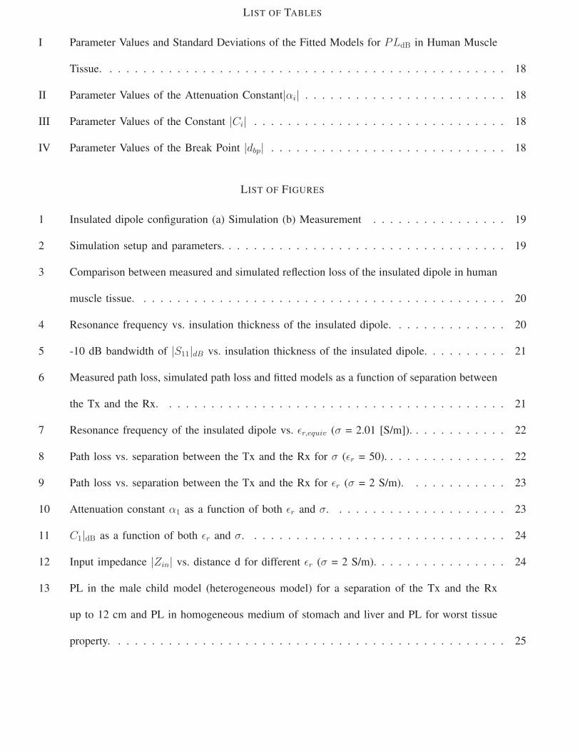
LIST OF TABLES

I Parameter Values and Standard Deviations of the Fitted Models for PLdB in Human Muscle

Tissue. . . . . . . . . . . . . . . . . . . . . . . . . . . . . . . . . . . . . . . . . . . . . . . . 18

II Parameter Values of the Attenuation Constant|αi| . . . . . . . . . . . . . . . . . . . . . . . . 18

III Parameter Values of the Constant |Ci| . . . . . . . . . . . . . . . . . . . . . . . . . . . . . . 18

IV Parameter Values of the Break Point |dbp| . . . . . . . . . . . . . . . . . . . . . . . . . . . . 18

LIST OF FIGURES

1 Insulated dipole configuration (a) Simulation (b) Measurement . . . . . . . . . . . . . . . . 19

2 Simulation setup and parameters. . . . . . . . . . . . . . . . . . . . . . . . . . . . . . . . . . 19

3 Comparison between measured and simulated reflection loss of the insulated dipole in human

muscle tissue. . . . . . . . . . . . . . . . . . . . . . . . . . . . . . . . . . . . . . . . . . . . 20

4 Resonance frequency vs. insulation thickness of the insulated dipole. . . . . . . . . . . . . . 20

5 -10 dB bandwidth of |S11|dB vs. insulation thickness of the insulated dipole. . . . . . . . . . 21

6 Measured path loss, simulated path loss and fitted models as a function of separation between

the Tx and the Rx. . . . . . . . . . . . . . . . . . . . . . . . . . . . . . . . . . . . . . . . . 21

7 Resonance frequency of the insulated dipole vs. ǫr,equiv (σ = 2.01 [S/m]). . . . . . . . . . . . 22

8 Path loss vs. separation between the Tx and the Rx for σ (ǫr = 50). . . . . . . . . . . . . . . 22

9 Path loss vs. separation between the Tx and the Rx for ǫr (σ = 2 S/m). . . . . . . . . . . . 23

10 Attenuation constant α1 as a function of both ǫr and σ. . . . . . . . . . . . . . . . . . . . . 23

11 C1|dB as a function of both ǫr and σ. . . . . . . . . . . . . . . . . . . . . . . . . . . . . . . 24

12 Input impedance |Zin| vs. distance d for different ǫr (σ = 2 S/m). . . . . . . . . . . . . . . . 24

13 PL in the male child model (heterogeneous model) for a separation of the Tx and the Rx

up to 12 cm and PL in homogeneous medium of stomach and liver and PL for worst tissue

property. . . . . . . . . . . . . . . . . . . . . . . . . . . . . . . . . . . . . . . . . . . . . . . 25

TABLE I

PARAMETER VALUES AND STANDARD DEVIATIONS OF THE FITTED MODELS FOR PLdB IN HUMAN MUSCLE TISSUE.

Parameter αi[1

cm] Ci[dB] Standard Deviation[dB] devimax[dB] deviavg[dB]

Model of (2) 0.99 7.18 0.15 0.56 0.26

Model of (3) 0.66 15.79 0.28 1.22 0.40

TABLE II

PARAMETER VALUES OF THE ATTENUATION CONSTANT|αi|

Parameter Ai Bi Di Ei Fi Relative Error [%]

Model of (6) 7.19 -0.04 4.86 0.05 0.05 3.9 %

Model of (7) 3.02 -0.04 1.83 0.11 0.07 3.5 %

TABLE III

PARAMETER VALUES OF THE CONSTANT |Ci|

Parameter Ui Vi Wi Xi Yi σi[dB]

Model of (8) 1.98 -22.11 0.66 -1.05 6.56 0.52

Model of (9) 0.47 -28.59 0.55 -2.24 21.18 0.33

TABLE IV

PARAMETER VALUES OF THE BREAK POINT |dbp|

Parameter Pi Qi Ri Si Ti Relative Error [%]

Model of |dbp| 0.29 0.01 4.83 0.30 0.68 7.3 %

Insulation

Dipole (PEC)

Voltage source

(a) (b)

Insulation

Dipole (PEC)

Stub

Coaxial cable connected to NWA

Sleeve

Fig. 1. Insulated dipole configuration (a) Simulation (b) Measurement

Fig. 2. Simulation setup and parameters.

1 1.5 2 2.5 3 3.5 4−25

−20

−15

−10

−5

0

Frequency [GHz]

S11 [dB

]

Measurement

SEMCAD

FEKO

Fig. 3. Comparison between measured and simulated reflection loss of the insulated dipole in human muscle tissue.

0 0.5 1 1.5 2 2.5 3 3.5 4 4.50.8

1

1.2

1.4

1.6

1.8

2

2.2

2.4

2.6

f res[G

Hz]

t [mm]

Fig. 4. Resonance frequency vs. insulation thickness of the insulated dipole.

0 0.5 1 1.5 2 2.5 3 3.5 4 4.50.2

0.3

0.4

0.5

0.6

0.7

0.8

0.9

BW

[G

Hz]

t [mm]

Fig. 5. -10 dB bandwidth of |S11|dB vs. insulation thickness of the insulated dipole.

0 1 2 3 4 5 6 7 810

20

30

40

50

60

70

d [cm]

PL [dB

]

Measurement

Model of (2)

Model of (3)

Semcad

Feko

Fig. 6. Measured path loss, simulated path loss and fitted models as a function of separation between the Tx and the Rx.

2.8 3 3.2 3.4 3.6 3.8 41.95

2

2.05

2.1

2.15

2.2

2.25

2.3

2.35

f res [G

Hz]

εr,equiv

Fig. 7. Resonance frequency of the insulated dipole vs. ǫr,equiv (σ = 2.01 [S/m]).

0 1 2 3 4 5 6 7 810

20

30

40

50

60

70

80

90

d [cm]

PL [dB

]

σ = 0.5 S/m

σ = 1 S/m

σ = 1.5 S/m

σ = 2 S/m

σ = 2.5 S/m

σ = 3 S/m

σ = 3.5 S/m

Fig. 8. Path loss vs. separation between the Tx and the Rx for σ (ǫr = 50).

0 1 2 3 4 5 6 7 810

20

30

40

50

60

70

80

90

100

110

d [ cm]

PL

[d

B]

εr = 5

εr = 15

εr = 25

εr = 35

εr = 45

εr = 55

εr = 65

Fig. 9. Path loss vs. separation between the Tx and the Rx for ǫr (σ = 2 S/m).

020

4060

80

0

2

40

0.5

1

1.5

2

2.5

3

εr σ [S/m]

α1 [1/c

m]

α1

Fit

Fig. 10. Attenuation constant α1 as a function of both ǫr and σ.

020

4060

80

0

2

4

0

5

10

15

εr σ [S/m]

C1 [dB

]

C1

Fit

Fig. 11. C1|dB as a function of both ǫr and σ.

0 1 2 3 4 5 6 7 846

48

50

52

54

56

58

60

62

d [cm]

Zin

[Ohm

]

εr = 30

εr = 40

εr = 50

εr = 60

Fig. 12. Input impedance |Zin| vs. distance d for different ǫr (σ = 2 S/m).

0 2 4 6 8 10 1210

20

30

40

50

60

70

80

90

100

110

d [cm]

PL [dB

]

PLVFB

PL Homogeneous Liver

PL Homogeneous Stomach

PL Worst−case Small Intestine

Fig. 13. PL in the male child model (heterogeneous model) for a separation of the Tx and the Rx up to 12 cm and PL in homogeneous

medium of stomach and liver and PL for worst tissue property.