near field sensing and antenna design for wireless body ... w... · near field sensing and antenna...
TRANSCRIPT

Near Field Sensing and Antenna
Design for Wireless Body Area Network
A thesis submitted to the School of Electrical and Electronic
Engineering for the degree of Doctor of Philosophy
By Waleed Amer
Newcastle University
Newcastle upon Tyne, UK
March 2016


To my ...
... supervisors, for their patience;
... friends, for their support;
...and family, for their prayers.

Certificate of Originality
I declare that this thesis is my own work and it has not been previously submitted by me or
by anyone else for a degree or diploma at any educational institute, school or university. To
the best of my knowledge, this thesis does not contain any previously published work, except
where the use of another person's work has been cited and included in the list of references.
…………………………………………..
…………………………………………..

i
Abstract
Wireless body area network (WBAN) has emerged in recent years as a special class of
wireless sensor network; hence, WBAN inherits the wireless sensor network challenges
of interference by passive objects in indoor environments. However, attaching wireless
nodes to a person’s body imposes a unique challenge, presented by continuous changes
in the working environment, due to the normal activities of the monitored personnel.
Basic activities, like sitting on a metallic chair or standing near a metallic door, drastically
change the antenna behaviour when the metallic object is within the antenna near field.
Although antenna coupling with the human body has been investigated by many recent
studies, the coupling of the WBAN node antenna with other objects within the
surrounding environment has not been thoroughly studied.
To address the problems above, the thesis investigates the state-of-the art of WBAN,
eximanes the influence of metallic object near an antenna through experimental studies
and proposes antenna design and their applications for near field environments. This
thesis philosophy for the previously mentioned challenge is to examine and improve the
WBAN interaction with its surrounding by enabling the WBAN node to detect nearby
objects based solely on change in antenna measurements. The thesis studies the
interference caused by passive objects on WBAN node antenna and extracts relevant
features to sense the object presence within the near field, and proposes new design of
WBAN antenna suitable for this purpose.
The major contributions of this study can be summarised as follows. First, it observes
and defines the changes in the return loss of a narrow band antenna when a metallic object
is introduced in its near field. Two methods were proposed to detect the object, based on
the refelction coefficient and transmission coefficient of an antenna in free space. Then,
the thesis introduces a new antenna design that conforms to the WBAN requirements of
size, while achieving very low sensitivity to human body. This was achieved through
combining two opposite Vivaldi shapes on one PCB and using a metallic sheet to act as
a reflector, which minimised the antenna coupling with the human body and reduced the
radiation pattern towards the body. Finally, the proposed antennas were tested on several
human body parts with nearby metallic objects, to compare the change in antenna s-
parameters due to presence of the human body and presence of the metallic object. Based
on the measurements, basic statistical indicators and Principal Component Analysis were
proposed to detect object presense and estimate its distance. In conclusion, the thesis
successfully shows WBAN antenna’s ability to detect nearby metallic objects through a
set of proposed indicators and novel antenna design. The thesis is wrapped up by the
suggestion to investigate time domain features and modulated signal for future work in
WBAN near field sensing.

ii
Contents
Abstract ....................................................................................................................... i
Contents ..................................................................................................................... ii
List of Figures ........................................................................................................... vi
List of Tables ............................................................................................................. x
Nomenclature ............................................................................................................ xi
Chapter 1 Introduction ............................................................................................. 1
1.1 Chapter Outline ............................................................................................... 2
1.2 Challenges and Motivation: Near-Field Interference by Passive Objects in
WBAN Application....................................................................................................... 2
1.3 Aim and Objectives ........................................................................................ 4
1.4 Contributions to Knowledge of the Thesis ..................................................... 5
1.5 Publications Arising From This Research ...................................................... 6
1.6 Thesis Outline ................................................................................................. 6
Chapter 2 Background and Related Work ............................................................... 8
2.1 Chapter Outline ............................................................................................... 9
2.2 Antenna Theory Fundamentals ....................................................................... 9
2.2.1 Antenna Measurements ........................................................................... 9
2.2.2 Field Regions and the Friis Transmission Equation .............................. 10
2.2.3 Two Rays Model ................................................................................... 11
2.2.4 Skin Depth ............................................................................................. 12
2.2.5 Radiation Pattern of an Antenna in Front of a PEC Surface ................. 13
2.2.6 Antenna Impedance ............................................................................... 15
2.2.7 S-parameter and Two Ports Network Model ......................................... 15
2.3 Wireless Body Area Network: Definitions and Challenges ......................... 16
2.3.1 Physical Layer Protocols used in WBAN Applications ........................ 18
Contents
iii
2.3.1.1 IEEE 802.11 Standard........................................................................ 18
2.3.1.2 IEEE 802.15.4 Standard..................................................................... 18
2.3.1.3 IEEE 802.15.6 Standard..................................................................... 19
2.3.2 Antenna Requirements for WBAN ....................................................... 20
2.3.3 Designs and types of WBAN antenna ................................................... 21
2.4 Related Work in Antenna-Based Sensor Techniques and Applications ....... 21
2.4.1 Related Work in Far Field Sensing ....................................................... 21
2.4.1.1 Radio Tomographic Imaging ............................................................. 23
2.4.1.2 Gesture Recognition Using Wireless Singals .................................... 24
2.4.2 Related work in Near-Field Sensing ..................................................... 25
2.4.2.1 Vital Sign Detection Based on Antenna Reflection Coefficient........ 26
2.4.2.2 RFID Tag Antenna-Based Sensor...................................................... 28
2.4.3 Related Work in Near-Field Sensing Using Specially Designed Antenna
28
2.4.3.1 Touchless Radar Sensor ..................................................................... 29
2.4.3.2 Wrist Pulse Detection ........................................................................ 29
2.4.3.3 Pedestrian Protection Using Capacitive Sensor ................................. 30
2.5 Summary ....................................................................................................... 31
Chapter 3 Sensing Passive Objects in the Near Field of a Narrow Band Antenna 33
3.1 Chapter Outline ............................................................................................. 34
3.2 Metallic Object Near a Single Antenna – Experiment I ............................... 34
3.2.1 Test Setup of the Narrow Band Antenna with a Metallic Object .......... 34
3.2.2 Results of S-parameters Change with Distance.................................... 37
3.3 Detection of the Plate Distance to the Antenna, Based on the Reflection
Coefficient ................................................................................................................... 41
3.3.1 Validation of Results Using CST-Software .......................................... 41
3.3.2 Distance Estimation Based on Changes in S11 Magnitude .................... 46

Contents
iv
3.4 Object Location Classification Using Principal Component Analysis ......... 49
3.4.1 Principal Component Analysis (PCA) Classifier .................................. 49
3.4.2 Classification Methodology and Results ............................................... 49
3.4.3 Statistical Significance of PCA Results ................................................ 52
3.5 Metallic Object Near Two Adjacent Antennas – Experiment II .................. 54
3.6 Summary ....................................................................................................... 59
Chapter 4 Design and Implementation of a Low Sensitivity UWB Antenna for
WBAN Applications ....................................................................................................... 60
4.1 Chapter Outline ............................................................................................. 61
4.2 Background ................................................................................................... 61
4.3 Antenna Design Concept and Performance .................................................. 63
4.3.1 Proposed Antenna Structure .................................................................. 64
4.3.2 Parametric Study and Optimization ...................................................... 66
4.3.3 Reflector Effect and Reflector Parametric Study .................................. 67
4.3.4 Current distribution ............................................................................... 70
4.3.5 Parasitic Element ................................................................................... 72
4.3.6 Radiation Efficiency .............................................................................. 74
4.3.7 Group Delay .......................................................................................... 75
4.4 Implementation and Experimental Setup and Results .................................. 77
4.5 Human Hand Experiment ............................................................................. 80
4.6 Summary ....................................................................................................... 81
Chapter 5 Near-Field Sensing using the UWB WBAN Antenna .......................... 82
5.1 Chapter Outline ............................................................................................. 83
5.2 Background ................................................................................................... 84
5.3 Off-body Antenna Measurements with a Passive Object in the Near Field . 85
5.3.1 Experimental Setup for Off-body UWB Antenna with a Metallic Object
85

Contents
v
5.3.2 Results and Discussion for Off-body Antenna with Metallic Object .... 87
5.4 On-body Antenna Measurements ................................................................. 92
5.4.1 On-body Antenna Measurements without a Passive Object in the Near
Field 93
5.4.2 On-body Antenna Measurements with a Passive Object in the Near Field
97
5.5 Proposed indicators for object detection near an on-body antenna .............. 99
5.6 Classification methodology and results for on-body tests .......................... 101
5.7 Summary ..................................................................................................... 103
Chapter 6 Conclusions and Future Work ............................................................. 104
6.1 Conclusions ................................................................................................. 105
6.1.1 Near Field Sensing and WBAN State of the Art..................................... 105
6.1.2 Off-Body Near Field Sensing Using Low Profile Antenna .................... 105
6.1.3 Antenna Design and On-Body Near Field Sensing................................. 106
6.2 Future Work ................................................................................................ 107
References .............................................................................................................. 109
Appendix A: Principal Component Analysis ............................................................ 123
A.1 Data Preparation and Classification Algorithm .............................................. 123
A.2 MATLAB Code for PCA Calculation ............................................................ 125
A.3 MATLAB Code for Permutation Test ............................................................ 126

vi
List of Figures
Figure 1: Illustration of interaction scenarios between the WBAN nodes and metallic
object in the network environment .................................................................................... 3
Figure 2: Two ray RF propagation model ................................................................... 11
Figure 3: Normalised E-field at the receiver side ....................................................... 13
Figure 4: The half-wave dipole: (a) Current distribution I(z); (b) Radiation pattern F(θ)
......................................................................................................................................... 14
Figure 5: A half-wave dipole parallel to the PEC surface ........................................... 14
Figure 6: The E-plane pattern (xz pattern) for various distances d ............................. 15
Figure 7: Key components of a WBAN (adapted from [1]) ........................................ 17
Figure 8: Transmit spectrums for the widespread protocols used by WBAN applications
......................................................................................................................................... 19
Figure 9: Examples of recent designs for WBAN antennas (a) 3D antenna (adapted
from [6]), (b) in-the-ear spiral monopole antenna (adapted from [67]), (c) insole antenna
(adapted from [69]), (d) embroidered and woven antennas (adapted from [66]) ........... 22
Figure 10: RTI system description (adapted from [76]): (a) an illustration of an RTI
network; (b) a photograph of the deployed network with an participant; (c) constructed
images of attenuation in the wireless network. ............................................................... 24
Figure 11: WiSee system (adapted from [88]): (a) the proposed nine gestures for WiSee;
(b) frequency–time Doppler profiles of the gestures ...................................................... 25
Figure 12: Vital sign detection system (adapted from [94]): (a) measurement setup of
the proposed system; (b) photograph of the measurement setup with the antenna and the
coupler; (c) details of the modified transceiver with a power sensor at Port 4 ............... 27
Figure 13: RFID Tag Antenna-Based Sensor (adapted from [99]): (a) patch antenna
with a crack in its ground plane; (b) effect of a crack on S11 parameters of the patch ... 28
Figure 14: Project Soli from Google (adapted from [102]): (a) illustration of the system
concept; (b) radar-based gesture sensor; and (c) three examples of hand gestures
corresponding to volume-roll, volume-slider and click-button, respectively. ................ 29
Figure 15: Wrist pulse detection (adapted from [103]): (a) photograph of the resonator
implementation; (b) time domain data of the proposed system and piezoelectric reference
......................................................................................................................................... 30
Figure 16: Capacitive coupling with a pedestrian in front of the capacitive sensor
(adapted from [104]) ....................................................................................................... 31

List of Figures
vii
Figure 17: Chapter-3 layout ......................................................................................... 35
Figure 18: Experiment setup: (a) antenna and metal object picture; (b) setup illustration
......................................................................................................................................... 36
Figure 19: Setup layout (top view) shows the positions of the plate and the antennas37
Figure 20: S11 and S12 magnitudes (when no metal plate is used) ............................... 38
Figure 21: Magnitude of S-parameter at position p1: (a) S12 and (b) S11 .................... 39
Figure 22: Magnitude of S-parameter at position p2: (a) S12 and (b) S11 .................... 39
Figure 23: Magnitude of S-parameter at position p3: (a) S12 and (b) S11 .................... 39
Figure 24: S12 (left) and S11 (right) at selected distances for three positions: (a) p1, (b)
p2 and (c) p3 (the two vertical red lines represent the 2.4-GHz ISM band boundaries) 40
Figure 25: Dipole antenna and metal plate simulation model ..................................... 43
Figure 26: Antenna reflection coefficient vs. distance d (simulation run #1): ............ 43
Figure 27: Antenna reflection coefficient vs. plate thickness (simulation run #2): ..... 45
Figure 28: Antenna reflection coefficient vs. plate length (simulation run #3): (a) S11
response; (b) minimum value of each response; and (c) antenna resonant frequency of
each response .................................................................................................................. 45
Figure 29: Reflection coefficient magnitude for selected values of d: (a) measured and
(b) simulation .................................................................................................................. 46
Figure 30: Change with distance: (a) Fres vs distance, (b) Rmin vs distance, (c) Fres vs
Rmin and (d) Zd vs distance .............................................................................................. 48
Figure 31: PCA classification for plate location, using S-parameters (for clarity, only
distances larger than 5 cm are plotted) ............................................................................ 50
Figure 32: PCA classification for plate location, using extracted features of
S-parameters .................................................................................................................... 55
Figure 33: Distance measurement using two adjacent nodes ...................................... 55
Figure 34: Vrec(d,f) surface: (a) experimental and (b) simulation ............................... 56
Figure 35: Vrec(d,f) at selected distances ...................................................................... 58
Figure 36: Fourier Transform of signal in Figure 35: (a) 1 cm, (b) 50 cm and (c) 100 cm,
(Only the first 20 components are shown, as the rest are very close to zero). ................ 58
Figure 37: Relation of distance d and Vrec(d,f) change ................................................ 59
Figure 38: Flowchart of this chapter ............................................................................ 62
Figure 39: Antenna schematic: (a) bottom side, (b) top side and (c) reflector position
......................................................................................................................................... 65

List of Figures
viii
Figure 40: Proposed antenna (perspective view) ......................................................... 65
Figure 41: Reflection coefficient response for selected cases in the parametric study
instances .......................................................................................................................... 67
Figure 42: Proposed antenna: (a) without a reflector; (b) with a flat reflector; and (c)
with a curved reflector .................................................................................................... 68
Figure 43: Comparison of the reflector effects, without the parasitic elements: (a) XZ
radiation pattern at 4 GHz and (b) |S11| response ............................................................ 69
Figure 44: Parametric study of |S11| for reflector parameters: (a) dr = 5 mm, tr = 1 mm
and variable br; (b) br=5 mm, tr = 1 mm and variable dr; and (c) dr = 5 mm, br = 5 mm
and variable tr ................................................................................................................. 71
Figure 45: Current distribution of the reflector surface at (a) 4 GHz, (b) 7 GHz and (c)
10 GHz ............................................................................................................................ 71
Figure 46: Proposed antenna schematic with parasitic patches: (a) bottom side and
(b) top side ...................................................................................................................... 72
Figure 47: Parametric study of |S11| for parasitic patch parameters: (a) gap1 variable,
(b) gap2 variable, (c) gap3 variable and (d) gap4 variable ............................................ 73
Figure 48: |S11| response with and without parasitic elements .................................... 74
Figure 49: Antenna efficiency radiation with the effect of the reflector and the parasitic
elements: (a) radiation efficiency and (b) total efficiency (b). ....................................... 75
Figure 50: Group delay for the design with reflector (with and without parasitic
elements) ......................................................................................................................... 76
Figure 51: Simulated and measured antenna |S11| response ........................................ 78
Figure 52: Simulated vs measured radiation pattern in the YZ-plane at 4 GHz ......... 78
Figure 53: Measured radiation pattern in the XZ- (left) and YZ- (right) planes at (a) 4
GHz, (b) 7 GHz and (c) 10 GHz. .................................................................................... 79
Figure 54: Proposed antenna: (a) antenna picture; (b) on hand palm test position; and
(c) on arm test position.................................................................................................... 80
Figure 55: Measured |S11| response outside anechoic chamber, with and without the
human hand. .................................................................................................................... 80
Figure 56: Chapter-5 layout ......................................................................................... 84
Figure 57: Experiment setup: (a) antenna and metal object picture; (b) setup illustration
......................................................................................................................................... 86
Figure 58: Off-body test setup layout (top view) shows the positions of the plate and

List of Figures
ix
the antennas ..................................................................................................................... 86
Figure 59: S12 magnitude for Off-body antenna at position (a) p1, (b) p2 and (c) p3 . 88
Figure 60: S11 magnitude for Off-body antenna at position (a) p1, (b) p2 and (c) p3 . 89
Figure 61: Off-body antennas, S12 (left) and S11 (right), at selected distances for three
positions: (a) p1, (b) p2 and (c) p3 .................................................................................. 90
Figure 62: Minimum value of the S11 response with distance d, at position (a) p1, (b)
p2 and (c) p3.................................................................................................................... 91
Figure 63: Frequency corresponding to the minimum value of S11 responses, at
positions (a) p1, (b) p2 and (c) p3 ................................................................................... 91
Figure 64: Proposed antenna without a reflector: (a) top, (b) bottom and (c) perspective
view ................................................................................................................................. 92
Figure 65: Proposed antenna with a reflector: (a) top, (b) bottom, (c) side and
(d) perspective view ........................................................................................................ 92
Figure 66: Top view of on-body test setup inside anechoic chamber ......................... 93
Figure 67: Antenna on body location: (a) the positions of the antennas on several body
parts (b) three locations of on-shoulder test .................................................................... 94
Figure 68: On-body test results (hand, arm and shoulder) for the antenna with a reflector
(left) and without a reflector (right): (a) S11, (b) S12 ....................................................... 95
Figure 69: On-body test results (hand, hand with watch) for the antenna with a reflector
(left) and without a reflector (right): (a) S11 and (b) S12 ................................................. 96
Figure 70: On-body test results (three shoulder positions) for the antenna with a
reflector (left) and without a reflector (right): (a) S11 and (b) S12 ................................... 96
Figure 71: Layout (top view) of on-body test with metallic object ............................. 97
Figure 72: On-body test results with a metallic object at selected distances, for the
antenna with a reflector (left) and without a reflector (right): (a) S11 and (b) S12 ........... 98
Figure 73: On-body test results with a metallic object, for the antenna with a reflector
(left) and without a reflector (right): (a) S11 and (b) S12 ................................................. 98
Figure 74: rms feature for S11 vs distance d .............................................................. 100
Figure 75: peak-to-peak feature for S11 vs distance d ................................................ 100
Figure 76: S12 features vs distance d: (a) rms and (b) peak-to-peak .......................... 100
Figure 77: PCA classification for the antenna with a reflector ................................. 102
Figure 78: PCA classification for the antenna without a reflector ............................ 102

x
List of Tables
Table 1: Simulation specifications .............................................................................. 42
Table 2: Simulation run parameters ............................................................................. 42
Table 3: Features and their calculations ...................................................................... 51
Table 4: Description of antenna parameters ................................................................ 64
Table 5: Parametric study instances ............................................................................ 66
Table 6: Parameter values for the responses shown in Figure 3 ................................. 66
Table 7: Antenna parameters (mm) after optimisation ................................................ 67
Table 8: Parasitic patch parameters (mm) ................................................................... 73

xi
Nomenclature
BER Bit Error Rate
CSMA/CA Carrier Sense Multiple Access with Collision
Avoidance
DSSS Direct-Sequence Spread Spectrum
ECG Electrocardiogram
HBC Human Body Communications
IR-UWB Impulse Response Ultra-Wide Band
ISM Industrial, Scientific and Medical Radio Band
LOS Line Of Sight
LQI Link Quality Indicator
MAC Medium Access Control
NLOS Non-Line of Sight
OFDM Orthogonal Frequency-Division Multiplexing
P2P Pear to Peak
PCA Principal Components Analysis
PEC Perfect Electric Conductor
PHY Physical layer
RF Radio Frequency
RFID Radio Frequency Identifier
RL Return Loss
RMS Root Mean Square
RSSI Received Signal Strength Indicator
RTI Radio Tomographic Imaging
SHM Structure Health Monitoring
SNR Signal to Noise Ratio
UWB Ultra-Wide Band
VNA Vector Network Analyser
WBAN Wireless Body Area Network
WLAN Wireless Local Area Network
WSN Wireless Sensor Network


1
Chapter 1 INTRODUCTION
Chapter 1
2
1.1 Chapter Outline
A significant step in the development of a Wireless Body Area Network (WBAN) is
the implementation of the physical layer of the network, which requires a thorough
characterisation of the electromagnetic wave propagation and antenna behaviour near the
human body [1-4]. In this chapter, we explain the challenges that are facing current
technology in this area and the thesis plan to provide a solution. The next section presents
the challenges and motivation behind this work. Section 1.3 states the thesis aim and
objectives, while Section 1.4 lists this work’s contribution to knowledge. The publications
that arose from this research are listed in Section 1.5. Finally, the overall outline of the
thesis is presented in Section 1.6.
1.2 Challenges and Motivation: Near-Field Interference by Passive Objects in
WBAN Application
In recent years, many researchers presents extensive studies regarding the antenna
design for wearable application [5-8], antenna coupling with the human body [9-12] and
the WBAN channel modelling for both on-body [13-15] and off-body communication
[16, 17]. Like many types of wireless networks, the WBAN wireless channel suffers from
interference by active and passive elements. Active interference is caused by other RF
sources in the environment, such as microwave cooking, mobile phone networks or
adjacent WBAN users [18-22]. Passive interference is caused by passive objects in the
environment (ones that do not transmit an RF signal), e.g., furniture, walls, doors, etc.
[23, 24]. Based on the object location from the LOS, the transmitted signal suffers from
multipath distortion, due to a reflection and/or shadowing. The effects of passive objects
on the signal propagation are covered by the channel modelling process, where these
objects are usually considered to be placed within the far field of the wireless node
antenna.
However, attaching wireless nodes to a human body imposes another challenge that is
unique for the WBAN application, compared to other wireless networks. This challenge
is presented by a continuous change in the work environment, due to the normal activities
of the monitored personnel [25, 26]. As seen in Figure 1, basic activities, like sitting on a
chair or standing near a door made with a metallic material, bring the antenna into direct
contact with an electric conductor surface and drastically change the antenna behaviour,
especially when the metallic object is within the antenna near field. The coupling between
the antenna and an object is frequency dependent and directly related to the distance

Chapter 1
3
between them. Unlike the objects in the far field, passive objects within the radius of a
few wavelengths of the wireless node engage in near-field coupling with the node
antenna, which severely affects the antenna radiation properties and, hence, the
transmitted/received wireless signal. The existence of such passive objects within a
nearby WBAN node can be frequent and last for a relatively long period of time in such
a manner that it disturbs the basic mechanism of the network, such as the routing. More
significantly, it alters the power level of the received signal, which is vital in some
applications, such as localisation [27] and spectrum sensing [28], which depend on
power-based measurements to estimate distance and channel availability, respectively. It
is worth mentioning that, metallic proximity with a low profile antenna has been
investigated in many other literatures regarding Radio Frequency Identifier (RFID) tags
and near-field communications [29-31], however, the human body was not considered.
Figure 1: Illustration of interaction scenarios between the WBAN nodes and metallic
object in the network environment
Metallic
objects in
vicinity of
human body
WBAN nodes suffer
from unwanted
coupling with metallic
surface
Chapter 1
4
To overcome this challenge, antenna diversity [17, 32, 33], or multi-sensor fusion [3]
can be employed. In [34], a steerable antenna was proposed for reliable transmissions in
Wireless Sensor Network (WSN) but it is not practical for wearable technology. Antenna
diversity can be applied to WBAN through a different allocation of the nodes around the
human body; however, applying antenna diversity for a single node is not practical, due
to size restrictions. Similarly, multi-sensor fusion require the addition of other types of
sensors to the node, such as proximity sensors or visual sensors, which increased its cost.
Also, when using a proximity sensor, the sensor itself disturb the node’s antenna radiation
if it was fixed too close to the antenna, and it doesn’t sense the antenna problem if it is
fixed too far. Both solutions complicate the node structure and fail to tackle the root of
the problem.
A better solution is to make the node more ‘context-aware’ through comprehensive
analysing of the antenna measurements. Despite the importance of context-awareness in
WBAN applications, there are limited solutions available, particularly at the Medium
Access Control (MAC) layer [35-37]. Measurements, such as the Received Signal
Strength Indicator (RSSI), Link Quality Indicator (LQI) or Signal to Noise Ratio (SNR),
are used in several applications [28, 38, 39] to assess the channel quality or the
surrounding environment. However, these measurements are highly affected by near
field, to the extent that they will give an incorrect assessment. The next sections explain
the thesis aim and suggestions for facing challenges in this field of research.
1.3 Aim and Objectives
The aim of this thesis is to improve the interaction between WBAN and its surrounding
by enabling the WBAN node to sense the presence of nearby passive object and estimate
its distance to WBAN antenna based solely on change in antenna measurements. The
main objectives of this thesis can be outlined thusly:
1. Undertake a thorough review of several related systems and applications, including
near-field sensing, localisation of passive objects and context-aware antennas, as
well as a review of the art of WBAN antenna design.
2. Understand the near field influence of passive objects on antenna measurements
through experimental studies using a low profile dipole antenna widely used for
indoor wireless applications and a metallic plate to be used as a passive object.
Then, build a simulation model of a similar setup in CST Microwave Studio to
validate the experimental results.

Chapter 1
5
3. Analyse the antenna measurements at several object locations near the antenna to
extract features that can be used to indicate the object presence and relate the change
in antenna measurements to the distance to the metallic object within the near field.
4. Design and develop an Ultra-Wide Band (UWB) antenna that conforms to the
WBAN requirements of size while achieving very low sensitivity when it comes in
contact with the human body. Also, perform a parametric study and parameters
optimisation of the proposed antenna to achieve the required antenna performance.
5. Conduct on-body tests to validate and identify the proposed antenna performance
for on-body near field sensing through placing the antenna on several human body
parts while placing the metallic objects at several distances from the antenna. The
tests aim to compare the change in antenna measurements due to the human body
presence and the metallic object presence; Also, the tests aim to assess the on-body
antenna sensitivity to metallic object within the near field.
1.4 Contributions to Knowledge of the Thesis
In the achievement of the above research objectives, the following contributions have
been made:
After investigation of low profile antenna measurements nearby a metallic object
the work manage to quantify the changes in antenna return loss and draw a relation
between the changes in the antenna return loss and the distance to the object. The
relation depend on both magnitude and resonant frequency of the return loss,
obtained from experimental tests using a commercial 2.4GHz low profile antenna
in free space.
Based on the problems identifed, a novel UWB WBAN antenna has been designed
and fabricated. The antenna consists of two Vivaldi shapes and a curved reflector.
The antenna performance was tested off-body and on-body.
The role of the antenna reflector in increasing the antenna’s sensitivity to nearby
metallic objects while decreasing its sensitivity to the human body, was studied and
demonstrated through a set of on-body experimental setups.
Two features to estimate the distance between the proposed antenna and the nearby
metallic objects were proposed. These two features are extracted from the absolute
change in the frequency response of the antenna reflection coefficient using root
mean square and peak-to-peak values, respectively.
The use of Principal Component Analysis classifier was proposed to detect the
Chapter 1
6
passive object location relative to line of sight between two antennas. Frequency
response of the reflection coefficient and the transmission coefficient of one
antenna were fed to the classifier. The method showed promising results using the
narrow band antenna as well as the proposed UWB antenna.
1.5 Publications Arising From This Research
Journal Papers
J1. W. Amer, A. Sabaawi, J. Zhang, and G. Y. Tian, “A Compact Dual-Vivaldi
sensor-based UWB antenna for WBAN applications,” submitted to IEEE
Transactions on Antennas & Propagation.
Conference Papers
C1. W. Amer, G. Y. Tian, and C. Tsimenidis, "Sensing passive object existence
within an antenna near field based on return loss," in Antennas and Propagation
Conference (LAPC), 2014 Loughborough, 2014, pp. 400–404.
C2. W. Amer, G. Y. Tian, and C. Tsimenidis, "A novel, low profile, directional
UWB antenna for WBAN," in Antennas and Propagation Conference (LAPC),
2014 Loughborough, 2014, pp. 708–710.
1.6 Thesis Outline
This thesis is organised as follows. Chapter 2 presents the background information on
wireless body area network technology, protocols and applications. The chapter also
discusses the related works and the state of context in the area of the context-aware sensor
network and near-field sensing.
Chapter 3 presents a study of the effects of metallic objects on antenna measurements
within the near field. This is presented through a set of experiments inside an anechoic
chamber, using a low profile, narrow band antenna, and the results are validated through
simulation, using CST Microwave Studio. The chapter also analyses the change in the
antenna measurements and proposes several indicators to relate the changes in antenna
return loss to the distance between the antenna and the nearby object within the near field.
Chapter 4 presents the design concept and performance analysis of a novel UWB
WBAN antenna that is characterised by its low profile and low sensitivity to the human
body. Also, a parametric study of the antenna parameters is presented, as well as an
Chapter 1
7
investigation of the reflector effects on the antenna. Then the chapter presents an
experimental setup to test the antenna performance.
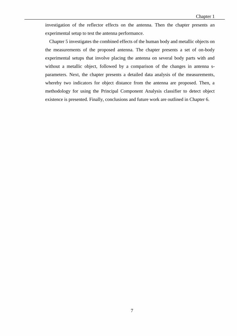
Chapter 5 investigates the combined effects of the human body and metallic objects on
the measurements of the proposed antenna. The chapter presents a set of on-body
experimental setups that involve placing the antenna on several body parts with and
without a metallic object, followed by a comparison of the changes in antenna s-
parameters. Next, the chapter presents a detailed data analysis of the measurements,
whereby two indicators for object distance from the antenna are proposed. Then, a
methodology for using the Principal Component Analysis classifier to detect object
existence is presented. Finally, conclusions and future work are outlined in Chapter 6.

8
Chapter 2 BACKGROUND AND RELATED
WORK

Chapter 2
9
2.1 Chapter Outline
This chapter presents theoretical background and state-of-the-art WBAN technology,
as a foundation to the following chapters of this thesis. Section 2.2 lists basic definitions
and theoretical background about antenna and wireless signal propagation, while
Section 2.3 defines the WBAN technology and related communication protocols, with an
emphasis on the physical layer issues. Finally, Section 2.4 presents a literature review of
recent related works. The literature review involves several examples of far field and
near-field sensing systems and their applications, as well as examples of studies about the
interaction between the human body and nearby passive objects in WBAN.
2.2 Antenna Theory Fundamentals
The following subsections present a brief background about antenna measurements,
antenna field regions and electromagnetic propagation models.
2.2.1 Antenna Measurements
There are several measurements to assess the performance of an antenna, depending on
the field of application where the antenna will be used. However, a good starting point in
the testing process of most antennas is to measure the antenna radiation pattern, antenna
efficiency and antenna gain. The antenna radiation pattern is defined as a mathematical
function or a graphical representation of the angular variation of radiation around the
antenna, typically in the far field [40]. The radiation pattern can be referenced as a specific
radiation component at a given polarisation or the absolute radiation of all the
components. The antenna efficiency term can refer to the number of efficiencies related
with the antenna, mainly, radiation efficiency (𝑒𝑐𝑑) and total efficiency (𝑒𝑇). Radiation
efficiency refers to the ratio of the radiated power to the accepted power fed to the antenna,
whereby the difference between the two values of power comes from conduction loss and
dielectric loss. On the other hand, total efficiency refers to the ratio of radiated power to
the input power fed to the antenna. In other words, the total efficiency of an antenna is
the radiation efficiency multiplied by the impedance mismatch loss (𝑒𝑟) of the antenna,
as given by [40]
𝑒𝑇 = 𝑒𝑟𝑒𝑐𝑑 = 𝑒𝑐𝑑(1 − Γ2) , (1)
where Γ is the voltage reflection coefficient at the input terminals of the antenna.

Chapter 2
10
Another useful measure describing the performance of an antenna is the gain. The gain
is defined as the ratio of the intensity, in a given direction, to the radiation intensity that
would be obtained if the power accepted by the antenna were radiated isotopically. When
the direction is not stated, the power gain is usually considered in the direction of
maximum radiation [40].
2.2.2 Field Regions and the Friis Transmission Equation
The space around an antenna can be divided into two regions, based on the behaviour
of the transmitted signal: the far field and the near field. In the far-field region, the fields
exhibit local plane wave behaviour, and the transmission follows the Friis Equation, given
by [41]
𝑃𝑟
𝑃𝑡= (
𝜆
4𝜋𝑅)
2
𝐺𝑡𝐺𝑟 ,
(2)
where 𝑃𝑡 is the transmitted power, 𝑃𝑟 is the received power, 𝐺𝑡 and 𝐺𝑟 are the transmitting
and receiving antenna gains, respectively, and R is the distance between the two antennas.
The near-field region is closer to the antenna and is divided into a radiated near field,
where the radiation (real-valued) fields dominate over the reactive fields, and a reactive
near field, where the reactive fields dominate over the radiation fields near field. The
boundaries of these regions depend on the transmitted signal wavelength (λ) and the
antenna’s largest dimension (D). However, the exact definitions of these boundaries
change from one antenna type to another [42].
For an electrically small antenna (defined as D/2 ≪λ), the radius, r, for each region
boundary is calculated as follows [42]:
𝑟𝑟𝑒𝑎𝑐𝑡𝑖𝑣𝑒 𝑛𝑒𝑎𝑟 𝑓𝑖𝑒𝑙𝑑 =𝜆
2π , (3)
𝜆
2π < 𝑟𝑟𝑎𝑑𝑖𝑎𝑡𝑒𝑑 𝑛𝑒𝑎𝑟 𝑓𝑖𝑒𝑙𝑑 ≤ 5 λ , (4)
𝑟𝑓𝑎𝑟 𝑓𝑖𝑒𝑙𝑑 > 5 𝜆. (5)
And for larger antenna, such that D>2.5λ, these boundaries become
𝑟𝑟𝑒𝑎𝑐𝑡𝑖𝑣𝑒 𝑛𝑒𝑎𝑟 𝑓𝑖𝑒𝑙𝑑 = 0.62√𝐷3/𝜆 , (6)
0.62√𝐷3/𝜆 < 𝑟𝑟𝑎𝑑𝑖𝑎𝑡𝑒𝑑 𝑛𝑒𝑎𝑟 𝑓𝑖𝑒𝑙𝑑 ≤
2𝐷2
λ , (7)
𝑟𝑓𝑎𝑟 𝑓𝑖𝑒𝑙𝑑 >2𝐷2
λ. (8)

Chapter 2
11
In the case of using a 1/4-wave dipole antenna that works in 2.4GHz, the antenna’s
electrical length (approximately 3cm) is considered small compared to the wavelength,
which is around 12cm; hence, the equation for an electrically small antenna should be
applied.
2.2.3 Two Rays Model
Obstacles placed near two communicating antennas usually reflect the radio wave
incident upon their surface and produce multipath components on the receiver’s side. The
received signal will be a combination of direct and reflected waves. In an indoor,
multipath-rich environment, the received signal can be greatly degraded by this effect.
Figure 2: Two ray RF propagation model
Figure 2 shows the two-ray propagation model, where two antennas are fixed near a
Perfect Electric Conductor (PEC) object or ground. The distance between the transmitting
and receiving antennas is d1, which also represents the Line OF Sight (LOS) component
path. On the other hand, d2 and d3 represent the distances between the object and the
transmitting and receiving antennas, respectively. The triangle d1, d2 and d3 lies in the
incidence wave plane. Then, the direct path d’ and indirect path d’’ can be defined as
[41]:
d’= d1 , (9)
d’’= d2 + d3 . (10)
Assuming the space around the antennas is free space and μ1 = μ2, the two ray model
can be simplified, and the total received E-field , ETOT, is then a result of the direct line-
of-sight component, ELOS, and the reflected component, EREFLECT. If E0 is the free space
E-field at a reference distance d0 from the transmitter, then for d>d0, the free space
propagating the E-field is given by 𝐸(𝑑, 𝑡). The E-field, due to the line-of-sight
d1
Transmitter
Receiver
d3
d2
ϕ
y x
z
PEC object

Chapter 2
12
component and reflection component at the fixed receiving antenna, can be expressed as
[41]
𝐸𝐿𝑂𝑆(𝑑′, 𝑡) =
𝐸0𝑑0
𝑑′cos (𝑤𝑐 (𝑡 −
𝑑′
𝑐)) ,
(11)
𝐸𝑅𝐸𝐹𝐿𝐸𝐶𝑇(𝑑", 𝑡) = Γ
𝐸0𝑑0
𝑑"cos (𝑤𝑐 (𝑡 −
𝑑"
𝑐)) ,
(12)
where Γ is the object reflection coefficient. For PEC at normal incidence, the reflection
coefficient (Γ) = -1. Assuming both antennas are vertically polarised, we obtain
𝐸𝑇𝑂𝑇(𝑑, 𝑡) =
𝐸0𝑑0
𝑑′cos (𝑤𝑐 (𝑡 −
𝑑′
𝑐))
+ (−1)𝐸0𝑑0
𝑑′′cos (𝑤𝑐 (𝑡 −
𝑑′′
𝑐)) .
(13)
If the object is very close to one antenna, then
∵ d1 ≈ d3 ≫ d2 . (14)
The amplitudes of Ed’ and Ed’’ are virtually identical and differ only in phase:
∴ | 𝐸0𝑑0
𝑑| ≈ |
𝐸0𝑑0
𝑑′ | ≈ |𝐸0𝑑0
𝑑′′ | , (15)
𝐸𝑇𝑂𝑇(𝑑, 𝑡) =
𝐸0𝑑0
𝑑( cos (𝑤𝑐 (𝑡 −
𝑑′
𝑐))
− cos (𝑤𝑐 (𝑡 −𝑑′′
𝑐)) ) ,
(16)
|𝐸𝑇𝑂𝑇(𝑑)| = 𝐸0𝑑0
𝑑√2 − 2 cos 𝜃 . (17)
Therefore, the received E-field, evaluated over frequency, shows oscillation, as in
Figure 3.
2.2.4 Skin Depth
The skin depth, δs, of the medium is the distance that characterizes how well an
electromagnetic wave can penetrate into a conducting medium, and it is calculated as
follow:
δ𝑠 = √ρ
𝜋𝑓𝜇0𝜇𝑟 (𝑚),
(18)

Chapter 2
13
where μ0 is the free space permeability which equals 4π * 10-7, μr is the relative
permeability of the medium, f is the frequency of the current in Hz, and ρ is the resistivity
of the medium in Ω .m. In a perfect dielectric, ρ =∞, therefore δs = ∞.Thus, in free space,
a plane wave can propagate with no loss in magnitude indefinitely. On the other extreme,
if the medium is a perfect conductor with ρ = 0, hence δs =0. For example, the iron. The
iron relative permeability is ranging from hundreds to hundreds of thousands based on its
purity. For pure iron with relative permeability equals to 4000, and resistivity equals to
0.1*10-6 Ω. m, the iron skin depth at 2.4GHz is δs ≈ 51.3*10-9 meter.
Figure 3: Normalised E-field at the receiver side
2.2.5 Radiation Pattern of an Antenna in Front of a PEC Surface
The current distribution for an omnidirectional dipole antenna placed vertically parallel
to the z-axis is shown in Figure 4. The radiation pattern in the XY-plane is a unit circle,
while the pattern in the XZ-plane is defined as [42]:
𝐹(𝜃) =cos [(
𝜋2) cos 𝜃]
sin 𝜃 .
(19)
To obtain the radiation pattern of the antenna in front of the PEC surface, image theory
is used to create an equivalent problem, yielding the same fields for z>0, by removing the
ground plane and introducing an image dipole of the same length, which is parallel to the
source dipole and equidistant from the PEC surface; thus, d=λ/2. This is shown in Figure
5, where the image dipole will have an amplitude excitation equal to the source dipole
and be 1800 out of phase. This can be modelled as an array antenna of two elements of
the same amplitude and opposite phase. Hence, the array factor is given by [42]:
Chapter 2
14
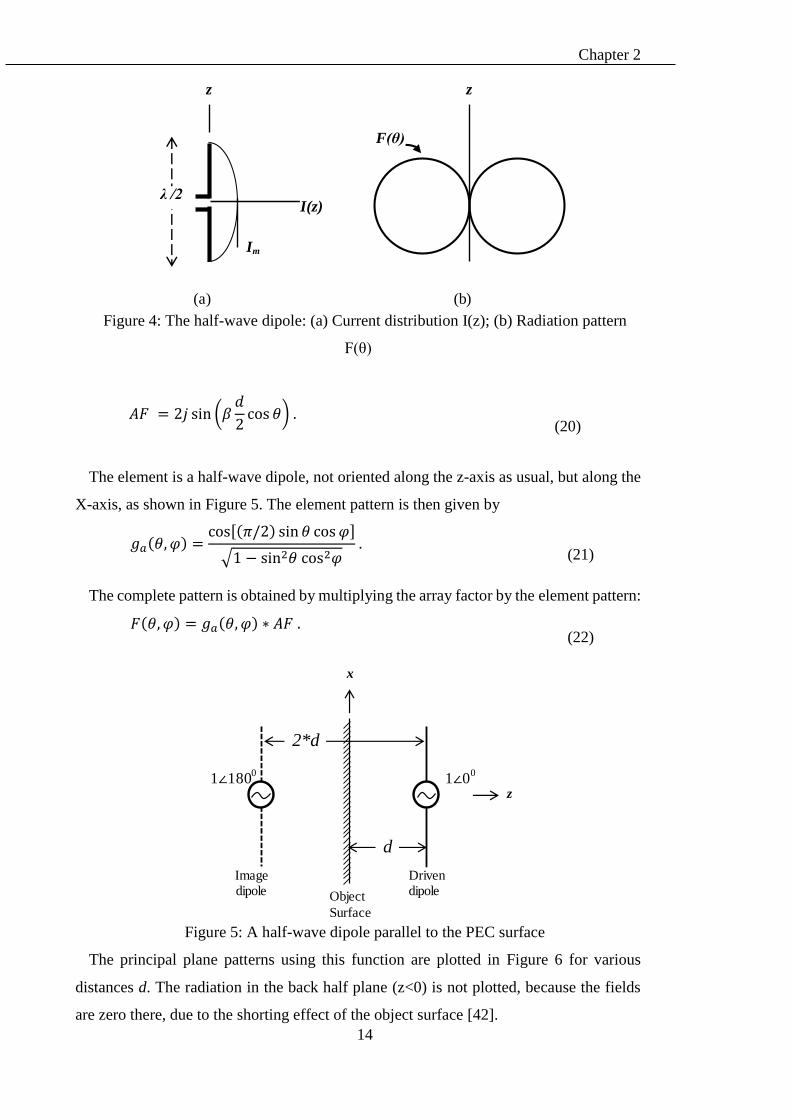
Figure 4: The half-wave dipole: (a) Current distribution I(z); (b) Radiation pattern
F(θ)
𝐴𝐹 = 2𝑗 sin (𝛽
𝑑
2cos 𝜃) .
(20)
The element is a half-wave dipole, not oriented along the z-axis as usual, but along the
X-axis, as shown in Figure 5. The element pattern is then given by
𝑔𝑎(𝜃, 𝜑) =
cos[(𝜋/2) sin 𝜃 cos 𝜑]
√1 − sin2𝜃 cos2𝜑 .
(21)
The complete pattern is obtained by multiplying the array factor by the element pattern:
𝐹(𝜃, 𝜑) = 𝑔𝑎(𝜃, 𝜑) ∗ 𝐴𝐹 .
(22)
Figure 5: A half-wave dipole parallel to the PEC surface
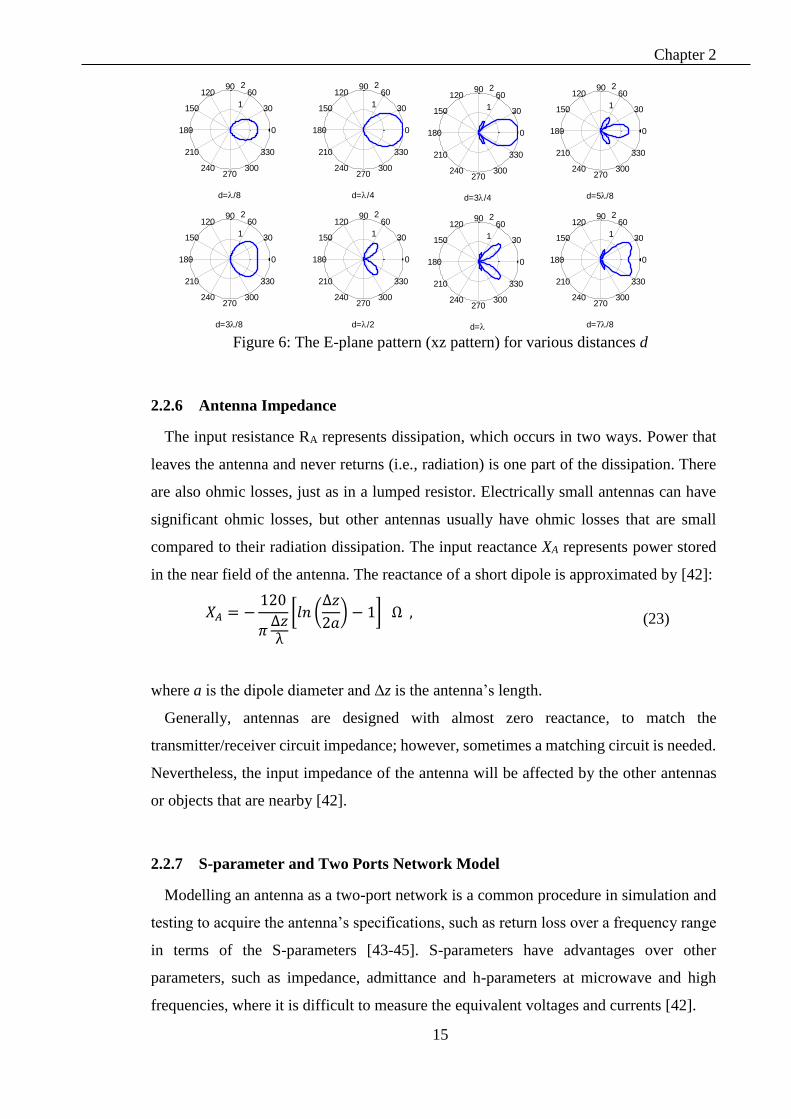
The principal plane patterns using this function are plotted in Figure 6 for various
distances d. The radiation in the back half plane (z<0) is not plotted, because the fields
are zero there, due to the shorting effect of the object surface [42].
λ /2
z z
F(θ)
(a) (b)
I(z)
Im
The half-wave dipole. (a) Current distribution I(z) . (b) Radiation pattern F(θ)
1∠00 1∠180
0
2*d
d
x
z
Driven dipole
Image dipole Object
Surface
Chapter 2
15
Figure 6: The E-plane pattern (xz pattern) for various distances d
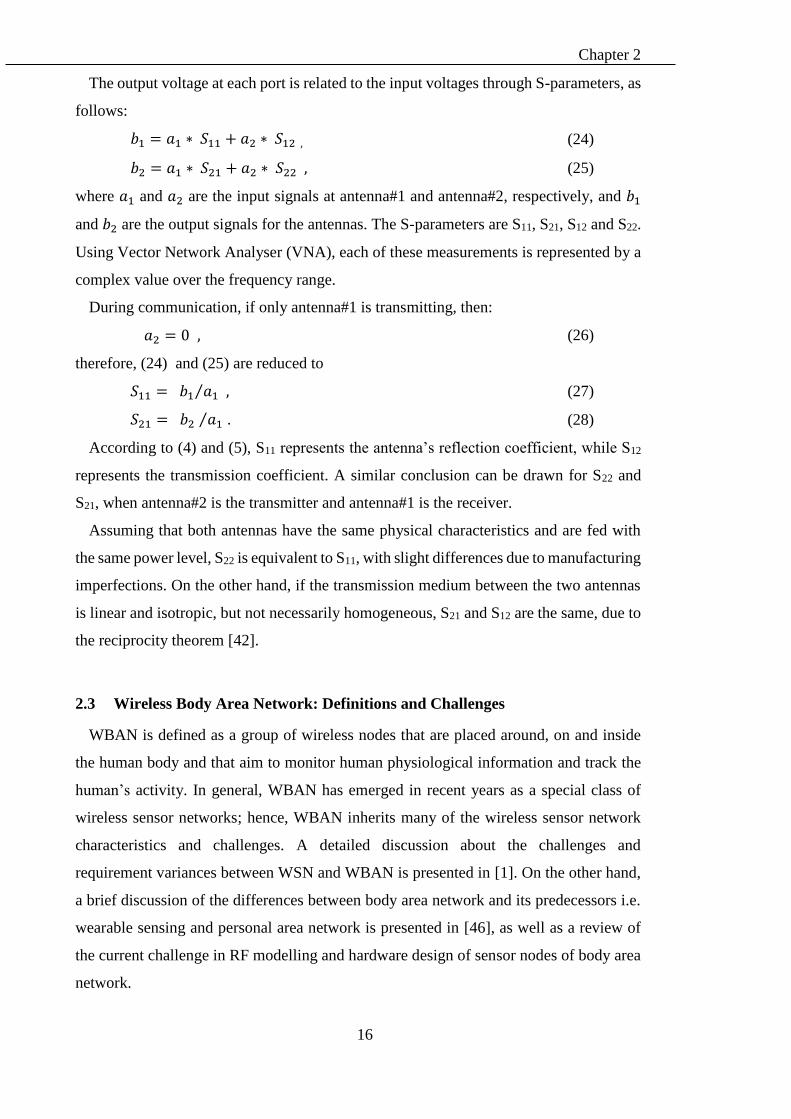
2.2.6 Antenna Impedance
The input resistance RA represents dissipation, which occurs in two ways. Power that
leaves the antenna and never returns (i.e., radiation) is one part of the dissipation. There
are also ohmic losses, just as in a lumped resistor. Electrically small antennas can have
significant ohmic losses, but other antennas usually have ohmic losses that are small
compared to their radiation dissipation. The input reactance XA represents power stored
in the near field of the antenna. The reactance of a short dipole is approximated by [42]:
𝑋𝐴 = −
120
𝜋∆𝑧λ
[𝑙𝑛 (∆𝑧
2𝑎) − 1] Ω , (23)
where a is the dipole diameter and Δz is the antenna’s length.
Generally, antennas are designed with almost zero reactance, to match the
transmitter/receiver circuit impedance; however, sometimes a matching circuit is needed.
Nevertheless, the input impedance of the antenna will be affected by the other antennas
or objects that are nearby [42].
2.2.7 S-parameter and Two Ports Network Model
Modelling an antenna as a two-port network is a common procedure in simulation and
testing to acquire the antenna’s specifications, such as return loss over a frequency range
in terms of the S-parameters [43-45]. S-parameters have advantages over other
parameters, such as impedance, admittance and h-parameters at microwave and high
frequencies, where it is difficult to measure the equivalent voltages and currents [42].
1
2
30
210
60
240
90
270
120
300
150
330
180 0
d=/8
1
2
30
210
60
240
90
270
120
300
150
330
180 0
d=/4
1
2
30
210
60
240
90
270
120
300
150
330
180 0
d=3/8
1
2
30
210
60
240
90
270
120
300
150
330
180 0
d=/2
1
2
30
210
60
240
90
270
120
300
150
330
180 0
d=5/8
1
2
30
210
60
240
90
270
120
300
150
330
180 0
d=3/4
1
2
30
210
60
240
90
270
120
300
150
330
180 0
d=7/8
1
2
30
210
60
240
90
270
120
300
150
330
180 0
d=
1
2
30
210
60
240
90
270
120
300
150
330
180 0
d=/8
1
2
30
210
60
240
90
270
120
300
150
330
180 0
d=/4
1
2
30
210
60
240
90
270
120
300
150
330
180 0
d=3/8
1
2
30
210
60
240
90
270
120
300
150
330
180 0
d=/2
1
2
30
210
60
240
90
270
120
300
150
330
180 0
d=5/8
1
2
30
210
60
240
90
270
120
300
150
330
180 0
d=3/4
1
2
30
210
60
240
90
270
120
300
150
330
180 0
d=7/8
1
2
30
210
60
240
90
270
120
300
150
330
180 0
d=
Chapter 2
16
The output voltage at each port is related to the input voltages through S-parameters, as
follows:
𝑏1 = 𝑎1 ∗ 𝑆11 + 𝑎2 ∗ 𝑆12 , (24)
𝑏2 = 𝑎1 ∗ 𝑆21 + 𝑎2 ∗ 𝑆22 , (25)
where 𝑎1 and 𝑎2 are the input signals at antenna#1 and antenna#2, respectively, and 𝑏1
and 𝑏2 are the output signals for the antennas. The S-parameters are S11, S21, S12 and S22.
Using Vector Network Analyser (VNA), each of these measurements is represented by a
complex value over the frequency range.
During communication, if only antenna#1 is transmitting, then:
𝑎2 = 0 , (26)
therefore, (24) and (25) are reduced to
𝑆11 = 𝑏1 𝑎1⁄ , (27)
𝑆21 = 𝑏2 𝑎1⁄ . (28)
According to (4) and (5), S11 represents the antenna’s reflection coefficient, while S12
represents the transmission coefficient. A similar conclusion can be drawn for S22 and
S21, when antenna#2 is the transmitter and antenna#1 is the receiver.
Assuming that both antennas have the same physical characteristics and are fed with
the same power level, S22 is equivalent to S11, with slight differences due to manufacturing
imperfections. On the other hand, if the transmission medium between the two antennas
is linear and isotropic, but not necessarily homogeneous, S21 and S12 are the same, due to
the reciprocity theorem [42].
2.3 Wireless Body Area Network: Definitions and Challenges
WBAN is defined as a group of wireless nodes that are placed around, on and inside
the human body and that aim to monitor human physiological information and track the
human’s activity. In general, WBAN has emerged in recent years as a special class of
wireless sensor networks; hence, WBAN inherits many of the wireless sensor network
characteristics and challenges. A detailed discussion about the challenges and
requirement variances between WSN and WBAN is presented in [1]. On the other hand,
a brief discussion of the differences between body area network and its predecessors i.e.
wearable sensing and personal area network is presented in [46], as well as a review of
the current challenge in RF modelling and hardware design of sensor nodes of body area
network.
Chapter 2
17
Figure 7: Key components of a WBAN (adapted from [1])
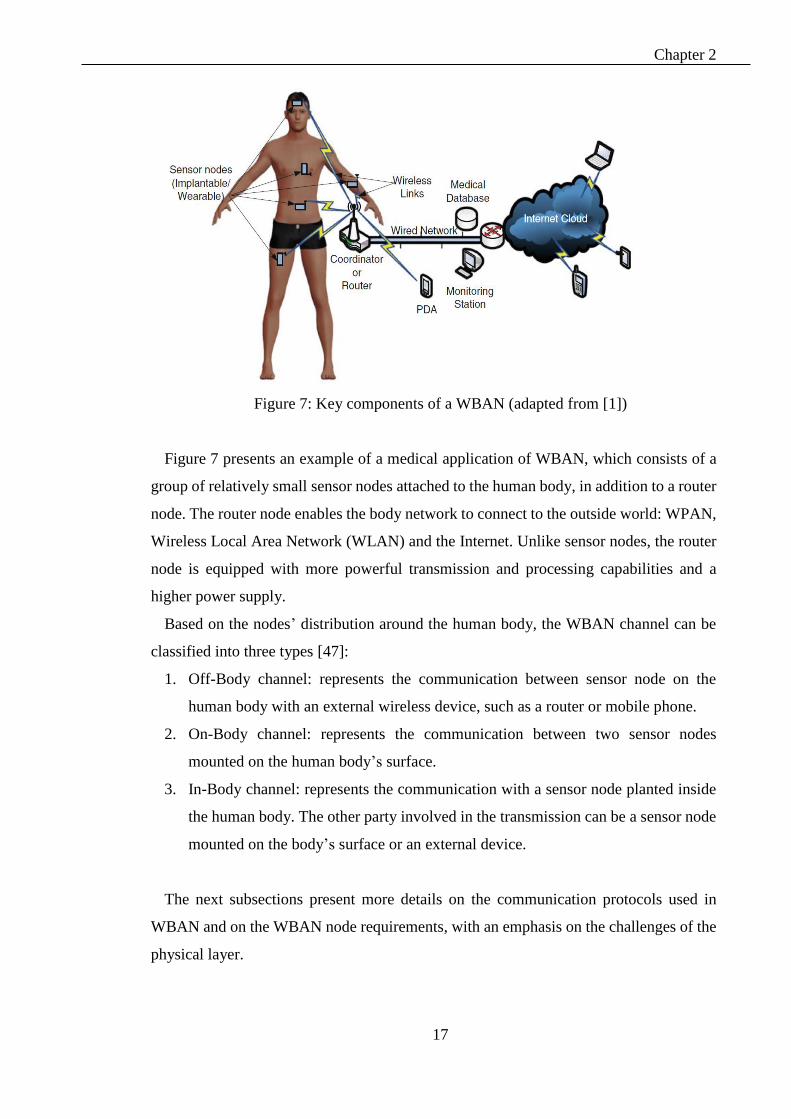
Figure 7 presents an example of a medical application of WBAN, which consists of a
group of relatively small sensor nodes attached to the human body, in addition to a router
node. The router node enables the body network to connect to the outside world: WPAN,
Wireless Local Area Network (WLAN) and the Internet. Unlike sensor nodes, the router
node is equipped with more powerful transmission and processing capabilities and a
higher power supply.
Based on the nodes’ distribution around the human body, the WBAN channel can be
classified into three types [47]:
1. Off-Body channel: represents the communication between sensor node on the
human body with an external wireless device, such as a router or mobile phone.
2. On-Body channel: represents the communication between two sensor nodes
mounted on the human body’s surface.
3. In-Body channel: represents the communication with a sensor node planted inside
the human body. The other party involved in the transmission can be a sensor node
mounted on the body’s surface or an external device.
The next subsections present more details on the communication protocols used in
WBAN and on the WBAN node requirements, with an emphasis on the challenges of the
physical layer.
Chapter 2
18
2.3.1 Physical Layer Protocols used in WBAN Applications
This section briefly discusses three wireless technologies that are widely used by the
WBAN research field: IEEE 802.11, IEEE 802.15.4 and IEEE 802.15.6.
2.3.1.1 IEEE 802.11 Standard
IEEE 802.11 is a set of media access control (MAC) and physical layer (PHY)
specifications for implementing wireless local area network (WLAN) computer
communication. Several variations of the standard are available, based on the used
frequency band. The standards 802.11b and 802.11g [48] work in the 2.4-GHz band,
while IEEE 802.11a [49] works in the 5-GHz band. Also, these standards use different
physical-layer communication mechanisms; for example, 802.11b and 802.11g control
their interference and susceptibility to interference by using direct-sequence spread
spectrum (DSSS) and orthogonal frequency-division multiplexing (OFDM) signalling
methods, respectively. In general, this standard has been implemented successfully in
many applications; however, it is rarely used for WBAN applications, due to its high
power requirements.
2.3.1.2 IEEE 802.15.4 Standard
IEEE 802.15.4 [50] is a standard that defines the physical layer and media access
control for low-rate, wireless personal area networks. It is maintained by the IEEE 802.15
working group, which defined the standard in 2003. The MAC layer of the IEEE 802.15.4
standard is based on Carrier Sense Multiple Access with Collision Avoidance
(CSMA/CA) for media access. The physical layer of the IEEE 802.15.4 standard supports
16 channels of 250 kbps each in 2.4 GHz, in addition to 10 channels of 40 kbps each in
915 MHz and one channel of 20 kbps in the 868-MHz band.
The IEEE 802.15.4 standard is usually used in conjugate with other standards, such as
ZigBee [51], which define the network, security and application layers. The ZigBee
network topology defines three levels of nodes: coordinator nodes, router nodes and end
devices. A ZigBee coordinator node initiates the network and manages network
resources. ZigBee router nodes enable multi-hop communication between the devices in
a network. Both coordinator and router nodes are supposed to have more reliable power
source and more hardware capabilities compared to the end devices. ZigBee’s end devices
communicate with parent nodes (router nodes or coordinator nodes) and operate with

Chapter 2
19
minimal functionality in order to reduce the power consumption. This standard is widely
used by many WSN and WBAN applications and research groups. Since both
IEEE802.11 and IEEE802.15.4 have been widely applied in many applications, several
research groups focused on studying the coexistence between the two standards in WSN
[52, 53] as well as WBAN [54, 55].
2.3.1.3 IEEE 802.15.6 Standard
Unlike the two standards explained earlier, the IEEE 802.15.6 [56] is proposed
specifically for (but not limited to) the use of the human body network. It defines three
physical layer specifications:
a. Narrow band communication, which consists of several channels available in
unlicensed frequency bands, such as the Industrial, Scientific and Medical
Radio (ISM) bands at 434MHz, 915 MHz and 2.45GHz, as well as the 403 MHz
band, which are used for medical implant communication services.
b. Ultra-wideband communication, where the UWB spectrum in the range of 3.1–
10 GHz is divided into eleven channels, with a channel bandwidth of 499.2
MHz for each channel.
c. Human Body Communications (HBC), whose signal carrier in the physical
layer is the electric current through the human body, instead of a wireless
electromagnetic transmission. It operates in the 21-MHz frequency band,
characterised by a 5.25-MHz bandwidth. The supported data rate ranges from
164 kbps to 1.3125 Mbps.
Figure 8: Transmit spectrums for the widespread protocols used by WBAN
applications
-41
UW
B E
IRP
(dB
m /
MH
z)
UWB
802.11a 802.11b/g
802.15.4
802.15.4
868 MHz 2.4GHz 5GHz 3.1GHz 10.6GHz

Chapter 2
20
Many aspects of IEEE 802.15.6 have been modified from its ancestor to fit the
requirements of a wearable implant network. For example, the scheduled access provides
guaranteed periodic access, allowing nodes to wake up at specific time intervals.
Therefore, it is suitable for medical data streaming applications e.g., Electrocardiogram
(ECG) waveform data streaming.
2.3.2 Antenna Requirements for WBAN
Antenna efficiency is typically the first requirement to consider with regard to selecting
an antenna in any application, yet different applications require different antenna
properties, such as directionality and power level. For WBAN, the human body’s
composition and the nature of the collected information impose some restrictions on the
antenna design, which are uniquely applied to this type of network.
These restrictions are:
Directional radiation pattern: Antennas mounted on the human body’s surface
are required to be omnidirectional and yet have minimum radiation towards the
human body [6, 57, 58].
Small size: small antenna dimensions are typically required for all WBAN
applications; however, the small size of the design affects the antenna radiation
efficiency for low frequencies and the antenna directionality [6, 58].
Vertically polarised: To maintain the minimum absorption of the signal by the
body tissues, the E-field of the transmitted signal is preferred to be
perpendicular to the human body’s surface [6, 7].
High fidelity factor: fidelity factor is a requirement for the communications and
measurements quality of the UWB impulse response [59-61].
In addition to the quantitative requirements listed above, most WBAN antennas
are required to meet some qualitative requirements, e.g., that they be flexible,
washable and durable. The antennas are also required to be unobtrusive, i.e.,
weaved into the user’s clothes or integrated with his/her accessories. This makes
the WBAN products more socially acceptable to wear, since in many medical
applications, a flashy distinctive design can cause feelings of stigma in the user
[57].

Chapter 2
21
2.3.3 Designs and types of WBAN antenna
Micro strip and loop designs are generally applied for on-body antennas because of
their conformability and light weight. However, for several on-body links (i.e., links
formed between on-body antennas placed on the user’s body), and for many body
postures, quarter-wavelength (λ/4) monopole antennas fixed on a small ground plane have
been shown to perform even better [2, 62]. The main reason is that the monopole antenna
exhibits an omnidirectional radiation pattern, which is highly preferable in cases where
the geometry and the characteristics of the wireless link are unknown [2] . Many recent
designs have been reported for WBAN applications and were showed to meet WBAN
requirements with regards to impedance and radiation pattern, e.g. PIFA antenna [63],
textile PIFA antenna [64], Loop antenna [65], embroidered and woven patch antennas
[66], and 3D antennas [6, 7]. On the other hand, some antenna design are specific for
application regarding its place on the human body such as user’s ear [14, 67], mouth [68],
and foot [69]. These antenna proposed generally for WBAN use and were tested using
model for skin or human torso. Figure 9 shows examples of designs for WBAN antennas
in recent literature.
2.4 Related Work in Antenna-Based Sensor Techniques and Applications
The use of radio wave to sense passive object presence is as old as the invention of
Radar systems [70-72] as well as the microwave imaging [73-75], and currently, several
researches proposed the use of antennas as sensors beside their typical function in the
communication process. This section review some of these researches and focus on the
works that employ low profile antenna. Based on the sensing range and the antenna type,
the next subsections discuss and classify recent works in the field of passive object
sensing into three categories. The first and second categories handle works that use low
profile antennas as sensors in the far field and the near field respectively. The third
category discusses recent works that use antennas specifically designed to serve as
sensors but not for communication process.
2.4.1 Related Work in Far Field Sensing
The acquisition of information about a passive object or phenomenon without making
physical contact with the object is a well-defined topic in the fields of radar systems and
remote sensing. However, the rise of WSN technology in the last decade and the
availability of miniaturised wireless nodes at low cost open the door to implementing RF-
based sensing and monitoring at a smaller level that fits in an indoor environment.

Chapter 2
22
Figure 9: Examples of recent designs for WBAN antennas (a) 3D antenna (adapted
from [6]), (b) in-the-ear spiral monopole antenna (adapted from [67]), (c) insole antenna
(adapted from [69]), (d) embroidered and woven antennas (adapted from [66])
(a)
(b)
(c)
(d)

Chapter 2
23
Such technology has many applications, ranging from touchless gaming controls to
pervasive indoor monitoring. It makes use of the abundance of nodes in a typical sensor
network to compensate for the low capabilities of each individual node. The details of
two recent cases that implement far field sensing in indoor environments are discussed
below.
2.4.1.1 Radio Tomographic Imaging
J. Wilson and N. Patwari proposed and designed a Radio Tomographic Imaging (RTI)
system [76, 77] for passive object monitoring, using commercially available WSN nodes.
Compared to other methods of monitoring, such as cameras, the RTI system provides a
better alternative, since the RF signals can travel through walls. RTI does not need a light
source; hence, it also can function in a dark environment. Moreover, the RTI system has
been useful for applications in which the location has been important, but the monitored
person has preferred for his or her identity to be unknown. Their suggested applications
for such systems included helping the correctional and law enforcement officers by
showing the location of people during indoor emergencies, such as hostage situations or
building fires. Also, they suggested that the system is convenient to control and monitor
‘smart homes’, where the operation cycles of heating and lighting systems are adapted to
human existence inside the building.
Their initial setup of the system consists of 28 wireless nodes distributed evenly along
the perimeter of a 6.4 × 6.4 m2, surrounding a total area of 41 m2. Each node is fixed on
a wooden stand, 1.5 m above the ground. Each node sends and receives signals from all
of the other nodes over the 2.4-GHz frequency band. Then, each pair of nodes sends the
value of the Received Signal Strength (RSS) of the link between them to a base station to
have the dada analysed. The RSS value is averaged over a 30-second period, which results
in approximately 100 RSS samples from each link. The presence of a human causes
shadowing to some of the links between the nodes. By solving the inverse problem for all
of the links, the human’s location can be determined. The results showed the ability of
the system to detect a human’s location within a 0.15-m accuracy. Figure 10 shows an
illustration of the RTI system and the final reconstructed image that displays the object’s
location. Later, the authors presented a modified version of the system to track a moving
object in an indoor environment, using a network fixed outside the building [78]. Also,
they presented a non-invasive respiration monitoring technique, which uses the same
technique to monitor the breathing of an otherwise stationary person [79]. The results

Chapter 2
24
showed that the breathing rate can be estimated within an error of 0.1 to 0.4 bpm, using
30 seconds of measurements.
It is worth to mention that the first attempt to use a low profile antenna as sensor in the
far field was presented by [80]. Similar systems that use the concept of wireless
tomography in WSN were independently presented in [81-83]. Moreover, a brief survey
of the wireless tomographic imaging can be found in [84-86]. Also, RF localization for
passive object was presented in [87] to achieve safe interaction scheme between human
and robot in industrial environment.
Figure 10: RTI system description (adapted from [76]): (a) an illustration of an RTI
network; (b) a photograph of the deployed network with an participant; (c) constructed
images of attenuation in the wireless network.
2.4.1.2 Gesture Recognition Using Wireless Singals
Qifan Pu and his colleagues presented a whole-home gesture recognition system, using
a wireless signal named WiSee [88]. Unlike commercially available systems, e.g., Kinect
(a) (b)
(c)

Chapter 2
25
[89], WiSee requires neither an infrastructure of cameras nor user instrumentation of the
devices.
Like the RTI system, Wisee enables applications in diverse domains, including home-
automation, elderly health care and gaming. Using a swiping hand motion in-air, a user
could control the music volume while showering, change the song playing on a music
system in the living room while cooking, or turn up the thermostat while in bed. However,
unlike the RTI system, WiSee doesn’t depend on the signal attenuation within a large
matrix of wireless nodes. Instead, it is based on a smaller number of nodes (typically Wi-
Fi transceivers) and uses the Doppler shift in the received signal as a signature to identify
the gesture. WiSee’s proof of concept was implemented in GNU Radio, using the USRP-
N210 hardware. Their results show that WiSee can identify and classify a set of nine
gestures with an average accuracy of 94%. Figure 11 shows the proposed gestures and
their corresponding Doppler shift signature. More information about the WiSee system
can be found on their website [90]. A similar technique presented by Microsoft Research
[91] provides a good example of human body interaction with its surrounding
environment, however it doesn’t use the antenna as sensor.
Figure 11: WiSee system (adapted from [88]): (a) the proposed nine gestures for
WiSee; (b) frequency–time Doppler profiles of the gestures
2.4.2 Related work in Near-Field Sensing
Near-field sensing takes place within the small region around the wireless device
antenna, typically less than a few wavelengths. Hence, near-field sensing techniques
(a) (b)
Push Dodge Strike
Pull Drag Kick
Circle Punch Bowling

Chapter 2
26
depend on the change in the antenna impedance, unlike the far field sensing techniques
that depend on far field measurements, such as multipath shadowing and Doppler shift.
The presence of objects or change of environmental conditions in the vicinity of an
antenna leads to a shift in both the phase and magnitude of the antenna resonant
frequency. Also, near-field sensing researches mainly focus on using measurements from
single nodes, rather than a fusion of data from many nodes, as in far field sensing
techniques. The details of selected recent researches of the near-field sensing techniques
are discussed below.
2.4.2.1 Vital Sign Detection Based on Antenna Reflection Coefficient
Many recent works studied the detection and monitoring of human vital signals, e.g.,
heartbeat rate and respiratory system rate, based on the change in a nearby wireless link.
These systems can detect vital signs from distances of 1 to 2 m. Some of these systems
depend on far field measurements, such as the direction of arrival [92] or Doppler shift
[93] of the received signals, while other depend on the antenna reflection coefficient [94,
95]. The far field measurements are highly affected by any slight human motion, which
results in unreliable measurements.
Yong-Jun and colleagues [94] presented a vital sign detection sensor, based on the
reflection coefficient variance from an antenna used in wireless communication devices.
Unlike other works, they used a vital sign detection scheme based on the magnitude
variation of the reflection coefficient from an antenna, so that it could be designed and
placed as a parasite component in a conventional transceiver system.
The characteristics of the reflection coefficient of a dipole antenna are used as
measurements of the vital signal in the near-field region. Since the human body has a
different permittivity than the air, placing a human subject in the near field of the antenna
shifts its resonant frequency and affects both the magnitude and phase of the reflection
coefficient. The antenna was designed and matched at the 2.4-GHz ISM band, and it was
connected to the base station through a 20-dB directional coupler and a power amplifier,
as shown in Figure 12. The antenna was placed at several distances, from 1 cm to 61 cm,
from a volunteer chest to cover the antenna near-field region. Their results showed close
matching, with the reference signal measured using a piezo-electric finger pressure sensor
for short distances. Analysing the data in the frequency domain showed the system’s
ability to correctly detect the heartbeat rate, even at 50 cm [94].

Chapter 2
27
Figure 12: Vital sign detection system (adapted from [94]): (a) measurement setup of
the proposed system; (b) photograph of the measurement setup with the antenna and the
coupler; (c) details of the modified transceiver with a power sensor at Port 4
(a)
(b)
(c)

Chapter 2
28
2.4.2.2 RFID Tag Antenna-Based Sensor
Following the success of RFID technology in many applications, a new trend of using
the antenna of the RFID tag as a sensor has emerged in recent years [96-98]. In addition
to its typical function as an identification tag, an RFID antenna can also be used as a
sensor to the attached objects, based on the change in the antenna impedance. Many recent
researches have employed this technique, mainly in structural health monitoring
applications [96].
The attached object usually acts as a ground plane for the tag; hence, cracks [99] and
strain [100] in the object surface or a change in the distance between the crack and the
tag [101] leads to a shift in the tag resonant frequency, which can be picked by the reader.
Figure 13 shows an example of crack detection, based on the change in the antenna
reflection coefficient.
Figure 13: RFID Tag Antenna-Based Sensor (adapted from [99]): (a) patch antenna with
a crack in its ground plane; (b) effect of a crack on S11 parameters of the patch
2.4.3 Related Work in Near-Field Sensing Using Specially Designed Antenna
The previous two subsections discussed related works that use low profile antennas and
RFID tags as sensors for passive objects. These antennas and RFID tags are commercially
available and widely used for wireless data transmission by many current wireless
devices. One the other hand, this subsection review the related works that use specially
designed antennas for near field sensing. The antennas in this case are meant to serve as
RF sensors, but not for wireless data transmission.
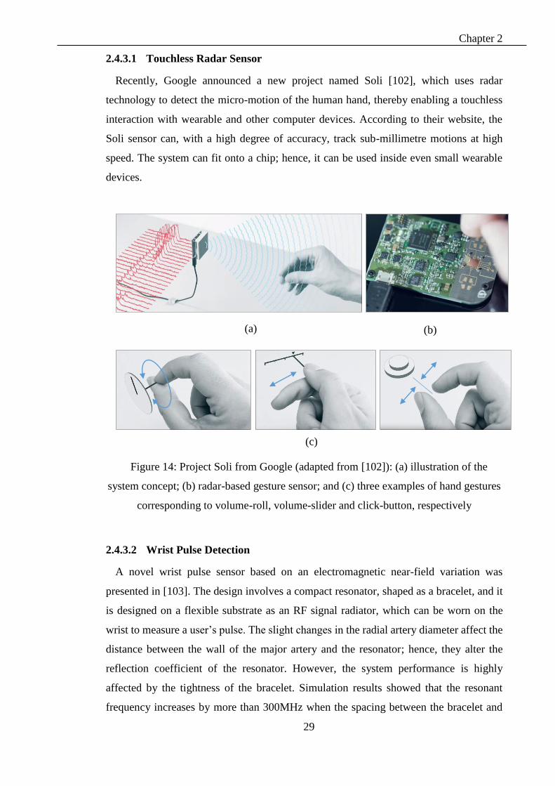
Chapter 2
29
2.4.3.1 Touchless Radar Sensor
Recently, Google announced a new project named Soli [102], which uses radar
technology to detect the micro-motion of the human hand, thereby enabling a touchless
interaction with wearable and other computer devices. According to their website, the
Soli sensor can, with a high degree of accuracy, track sub-millimetre motions at high
speed. The system can fit onto a chip; hence, it can be used inside even small wearable
devices.
Figure 14: Project Soli from Google (adapted from [102]): (a) illustration of the
system concept; (b) radar-based gesture sensor; and (c) three examples of hand gestures
corresponding to volume-roll, volume-slider and click-button, respectively
2.4.3.2 Wrist Pulse Detection
A novel wrist pulse sensor based on an electromagnetic near-field variation was
presented in [103]. The design involves a compact resonator, shaped as a bracelet, and it
is designed on a flexible substrate as an RF signal radiator, which can be worn on the
wrist to measure a user’s pulse. The slight changes in the radial artery diameter affect the
distance between the wall of the major artery and the resonator; hence, they alter the
reflection coefficient of the resonator. However, the system performance is highly
affected by the tightness of the bracelet. Simulation results showed that the resonant
frequency increases by more than 300MHz when the spacing between the bracelet and
(a) (b)
(c)

Chapter 2
30
the skin decreases to about 0.5 mm.
The system was designed to work at a 2.4-GHz ISM band. The experimental results
showed that the system sensitivity is comparable to a conventional piezoelectric or
photoplethysmography (PPG) sensor. Figure 15 (a) shows the system implementation,
while Figure 15 (b) shows the sensor measurement compared to the reference
measurement, using a piezoelectric sensor for finger pressure.
Figure 15: Wrist pulse detection (adapted from [103]): (a) photograph of the resonator
implementation; (b) time domain data of the proposed system and piezoelectric
reference
2.4.3.3 Pedestrian Protection Using Capacitive Sensor
A capacitive sensor for a pedestrian protection system in moving vehicles is presented
by [104]. The system is proposed to reduce the severity of injuries in the case of an
unavoidable frontal collision between a vehicle and a pedestrian. Although the system
doesn’t involve a wearable device, the design gives a good example of utilising the
coupling between the human body and nearby objects to enhance the interaction between
(a)
(b)
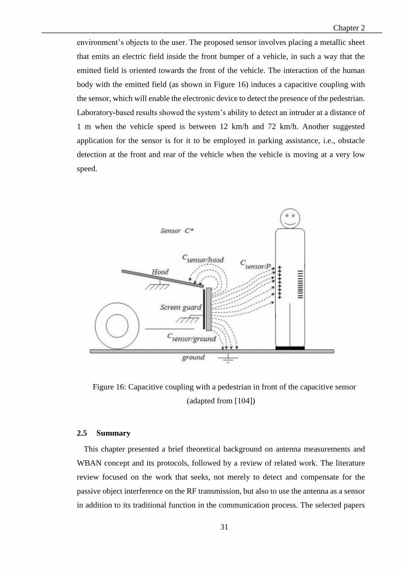
Chapter 2
31
environment’s objects to the user. The proposed sensor involves placing a metallic sheet
that emits an electric field inside the front bumper of a vehicle, in such a way that the
emitted field is oriented towards the front of the vehicle. The interaction of the human
body with the emitted field (as shown in Figure 16) induces a capacitive coupling with
the sensor, which will enable the electronic device to detect the presence of the pedestrian.
Laboratory-based results showed the system’s ability to detect an intruder at a distance of
1 m when the vehicle speed is between 12 km/h and 72 km/h. Another suggested
application for the sensor is for it to be employed in parking assistance, i.e., obstacle
detection at the front and rear of the vehicle when the vehicle is moving at a very low
speed.
Figure 16: Capacitive coupling with a pedestrian in front of the capacitive sensor
(adapted from [104])
2.5 Summary
This chapter presented a brief theoretical background on antenna measurements and
WBAN concept and its protocols, followed by a review of related work. The literature
review focused on the work that seeks, not merely to detect and compensate for the
passive object interference on the RF transmission, but also to use the antenna as a sensor
in addition to its traditional function in the communication process. The selected papers
Chapter 2
32
in the review section were classified into three categories: far field sensing, near field
sensing and near field sensing using specially designed antennas-like devices for the
sensing process but not for wireless data transmission.
WBAN nodes attached to human body suffer from the continuous changes in the
working environment, due to the normal activities of the human. This put node’s antenna
in frequent interaction with passive objects within the indoor environments and affect the
WBAN communication. The challenge in applying previously mention solutions
suggested by other authors, is that the WBAN antennas are, typically, designed to be less
sensitive to theirs surrounding to reduce the coupling with human body. This obstruct the
use of WBAN antenna as sensor for its surrounding. This leaves a gap for research in the
area of antenna design and near field interaction with passive object, human body, and
both as discussed by the next three chapters.
33
Chapter 3 SENSING PASSIVE OBJECTS IN
THE NEAR FIELD OF A NARROW BAND
ANTENNA
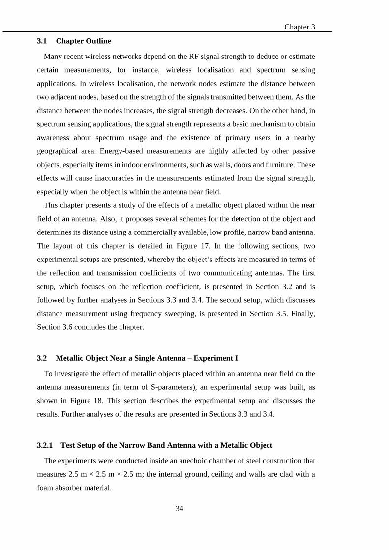
Chapter 3
34
3.1 Chapter Outline
Many recent wireless networks depend on the RF signal strength to deduce or estimate
certain measurements, for instance, wireless localisation and spectrum sensing
applications. In wireless localisation, the network nodes estimate the distance between
two adjacent nodes, based on the strength of the signals transmitted between them. As the
distance between the nodes increases, the signal strength decreases. On the other hand, in
spectrum sensing applications, the signal strength represents a basic mechanism to obtain
awareness about spectrum usage and the existence of primary users in a nearby
geographical area. Energy-based measurements are highly affected by other passive
objects, especially items in indoor environments, such as walls, doors and furniture. These
effects will cause inaccuracies in the measurements estimated from the signal strength,
especially when the object is within the antenna near field.
This chapter presents a study of the effects of a metallic object placed within the near
field of an antenna. Also, it proposes several schemes for the detection of the object and
determines its distance using a commercially available, low profile, narrow band antenna.
The layout of this chapter is detailed in Figure 17. In the following sections, two
experimental setups are presented, whereby the object’s effects are measured in terms of
the reflection and transmission coefficients of two communicating antennas. The first
setup, which focuses on the reflection coefficient, is presented in Section 3.2 and is
followed by further analyses in Sections 3.3 and 3.4. The second setup, which discusses
distance measurement using frequency sweeping, is presented in Section 3.5. Finally,
Section 3.6 concludes the chapter.
3.2 Metallic Object Near a Single Antenna – Experiment I
To investigate the effect of metallic objects placed within an antenna near field on the
antenna measurements (in term of S-parameters), an experimental setup was built, as
shown in Figure 18. This section describes the experimental setup and discusses the
results. Further analyses of the results are presented in Sections 3.3 and 3.4.
3.2.1 Test Setup of the Narrow Band Antenna with a Metallic Object
The experiments were conducted inside an anechoic chamber of steel construction that
measures 2.5 m × 2.5 m × 2.5 m; the internal ground, ceiling and walls are clad with a
foam absorber material.
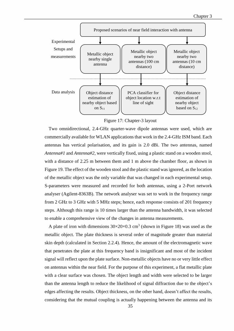
Chapter 3
35
Figure 17: Chapter-3 layout
Two omnidirectional, 2.4-GHz quarter-wave dipole antennas were used, which are
commercially available for WLAN applications that work in the 2.4-GHz ISM band. Each
antennas has vertical polarisation, and its gain is 2.0 dBi. The two antennas, named
Antenna#1 and Antenna#2, were vertically fixed, using a plastic stand on a wooden stool,
with a distance of 2.25 m between them and 1 m above the chamber floor, as shown in
Figure 19. The effect of the wooden stool and the plastic stand was ignored, as the location
of the metallic object was the only variable that was changed in each experimental setup.
S-parameters were measured and recorded for both antennas, using a 2-Port network
analyser (Agilent-8363B). The network analyser was set to work in the frequency range
from 2 GHz to 3 GHz with 5 MHz steps; hence, each response consists of 201 frequency
steps. Although this range is 10 times larger than the antenna bandwidth, it was selected
to enable a comprehensive view of the changes in antenna measurements.
A plate of iron with dimensions 30×20×0.3 cm3 (shown in Figure 18) was used as the
metallic object. The plate thickness is several order of magnitude greater than material
skin depth (calculated in Section 2.2.4). Hence, the amount of the electromagnetic wave
that penetrates the plate at this frequency band is insignificant and most of the incident
signal will reflect upon the plate surface. Non-metallic objects have no or very little effect
on antennas within the near field. For the purpose of this experiment, a flat metallic plate
with a clear surface was chosen. The object length and width were selected to be larger
than the antenna length to reduce the likelihood of signal diffraction due to the object’s
edges affecting the results. Object thickness, on the other hand, doesn’t affect the results,
considering that the mutual coupling is actually happening between the antenna and its
Experimental
Setups and
measurements
Data analysis
Proposed scenarios of near field interaction with antenna
Metallic object
nearby single
antenna
Metallic object
nearby two
antennas (100 cm
distance)
Metallic object
nearby two
antennas (10 cm
distance)
Object distance
estimation of
nearby object based
on S11
PCA classifier for
object location w.r.t
line of sight
Object distance
estimation of
nearby object
based on S12
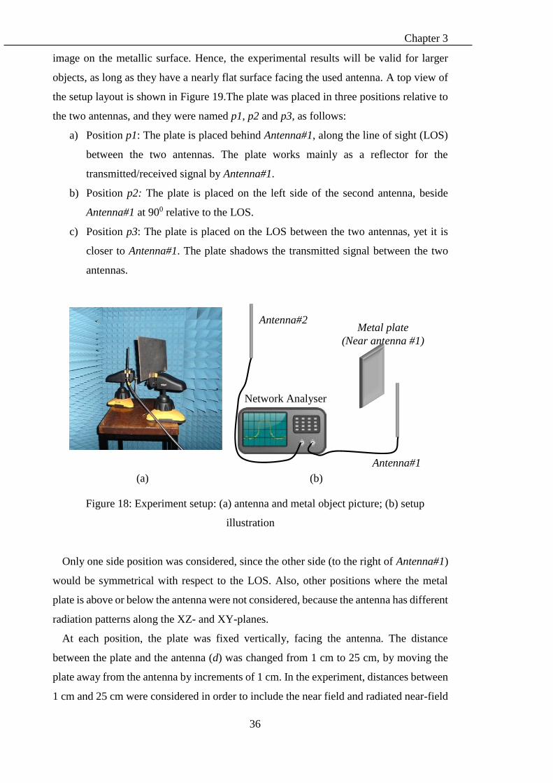
Chapter 3
36
image on the metallic surface. Hence, the experimental results will be valid for larger
objects, as long as they have a nearly flat surface facing the used antenna. A top view of
the setup layout is shown in Figure 19.The plate was placed in three positions relative to
the two antennas, and they were named p1, p2 and p3, as follows:
a) Position p1: The plate is placed behind Antenna#1, along the line of sight (LOS)
between the two antennas. The plate works mainly as a reflector for the
transmitted/received signal by Antenna#1.
b) Position p2: The plate is placed on the left side of the second antenna, beside
Antenna#1 at 900 relative to the LOS.
c) Position p3: The plate is placed on the LOS between the two antennas, yet it is
closer to Antenna#1. The plate shadows the transmitted signal between the two
antennas.
Figure 18: Experiment setup: (a) antenna and metal object picture; (b) setup
illustration
Only one side position was considered, since the other side (to the right of Antenna#1)
would be symmetrical with respect to the LOS. Also, other positions where the metal
plate is above or below the antenna were not considered, because the antenna has different
radiation patterns along the XZ- and XY-planes.
At each position, the plate was fixed vertically, facing the antenna. The distance
between the plate and the antenna (d) was changed from 1 cm to 25 cm, by moving the
plate away from the antenna by increments of 1 cm. In the experiment, distances between
1 cm and 25 cm were considered in order to include the near field and radiated near-field
Metal plate
(Near antenna #1)
Antenna#1
Network Analyser
Antenna#2
(a) (b)

Chapter 3
37
areas.
Figure 19: Setup layout (top view) shows the positions of the plate and the antennas
3.2.2 Results of S-parameters Change with Distance
The s-parameters, generated using the network analyser for the two antennas, consist
of: S11, S21, S12 and S22. Each one of them is a complex value (magnitude and phase).
However, in the discussion below, only the magnitude values of the S11 and S12
parameters are considered. The parameters S11 and S12 correspond to the reflection
coefficient and transmission coefficient, respectively, at Antenna#1. Since Antenna#2 is
relatively far (more than 2 meters) away from the metal plate, the plate has little or no
effect on the S22 value. Similarly, the transmission coefficients S21 and S12 are identical,
even when the object was introduced, due to transmission reciprocity [42]. At first, the
S-parameters were recorded without the presence of a metal plate. Then the metallic
object was introduced at several locations.
Figure 20 shows the magnitude of S11 and S12 before the metal object was placed. Since
the test used a narrow band antenna, the minimum value of S11 was between 2.4GHz and
2.5GHz, as expected, while S12 shows the maximum value in this frequency range. The
magnitude of S12 in this region depends mainly on the antenna gain and the distance
between the two antennas. Figure 21 shows the magnitudes of S11 and S12 at position p1
as functions of distance d and frequency. Similarly, Figure 22 and Figure 23 show the
results for positions p2 and p3, respectively. For more clarification, additional results are
presented in Figure 24, in 2D form, for selected instances of distance d.
2.2m
p3
d
Antenna#2
Antenna#1
p2
p1

Chapter 3
38
Figure 20: S11 and S12 magnitudes (when no metal plate is used)
The effects on the S12 magnitude range from a frequency-selected attenuation when the
object is at position p1, to severe shadowing for small distances at position p3, as
explained below:
a) At position p1, the metallic plate acteds as a reflector behind Antenna#1. Hence,
Antenna#1 received two copies of the transmitted signal from Antenna#2, the LOS
component and the NLOS component (reflected from the plate). The interference
between these two components appears as a frequency-dependent interference on
the Antenna#1 side. As the distance d increases, the response shows constructive
and destructive interferences for different distance values. The difference between
the constructive and destructive interferences is about 20 dB, and the distance
between two consecutive peaks is about 6 cm.
b) At position p2, the metallic plate is still acting as a reflector, but the interference
is less than that of p1. The distance between two consecutive peaks is about 15
cm in distance and 10 dB in value.
c) At position p3, the metal plate blocks the transmitted signal and causes a severe
reduction in transmitted power (≈20db) in the first 5cm, as well as a high
fluctuation in the S12 value. As the metal plate was moved away from the antenna,
the S12 value increased and tend to be steady. For distances greater than 20cm, the
effect vanishes and the value settles on its free space magnitude as shown in
Figure 23 (a). Although the metallic plate is still inside the Fresnel Zone, the
excess path loss (caused by sharp edge interference) is not noticeable.
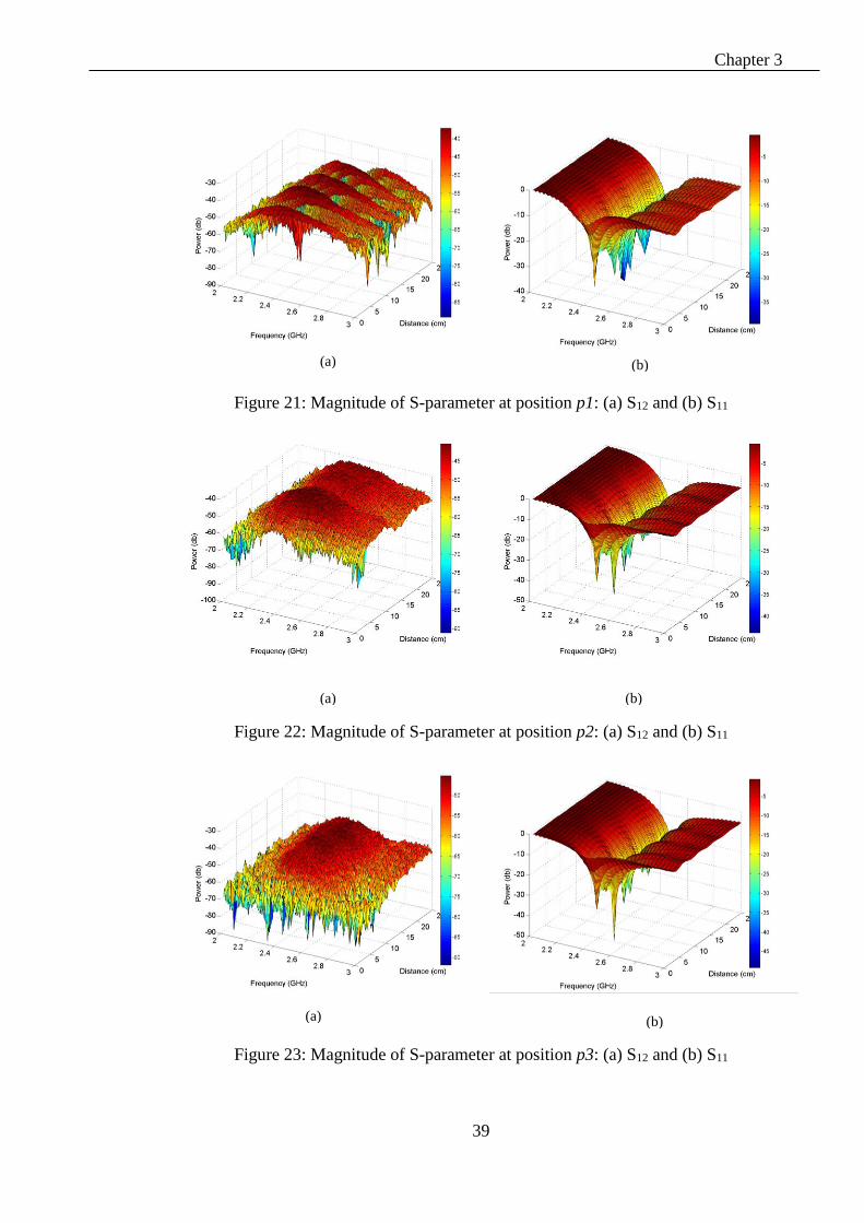
Chapter 3
39
Figure 21: Magnitude of S-parameter at position p1: (a) S12 and (b) S11
Figure 22: Magnitude of S-parameter at position p2: (a) S12 and (b) S11
Figure 23: Magnitude of S-parameter at position p3: (a) S12 and (b) S11
(a) (b)
(a) (b)
(a) (b)
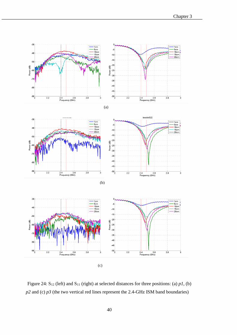
Chapter 3
40
Figure 24: S12 (left) and S11 (right) at selected distances for three positions: (a) p1, (b)
p2 and (c) p3 (the two vertical red lines represent the 2.4-GHz ISM band boundaries)
(a)
(b)
(c)

Chapter 3
41
For S11, the effects of the metallic object on the three positions are identical, except for
slight changes (<1 dB) due to setup differences. This is because the antenna used in the
experiment is omnidirectional in the H-plane. For small distances (d < 5 cm), the antenna
is unable to transmit correctly, due to high coupling between the antenna and the metallic
object, which makes the reflection coefficient above -10dB. For greater distances (d ≥ 5
cm), the response of S11 at resonant frequency drops below -10dB. As the distance d
increases, both the minimum value of the S11 response and its corresponding resonant
frequency are affected. A further analysis of the S11 response is presented in the following
section.
3.3 Detection of the Plate Distance to the Antenna, Based on the Reflection
Coefficient
The results in the previous section showed that placing a metallic object near an antenna
at distance d affects the antenna reflection coefficient, regardless of the object location
with respect to the LOS between the two antennas. As the distance d changes, the antenna
resonant frequency is shifted and the antenna reflection coefficient value is changed. By
analysing these two parameters, an object’s presence can be sensed, along with its relative
distance to the antenna. Hence, this section investigates the ability of a single antenna to
detect a metallic object’s existence within the near field and estimate d, based solely on
the reflection coefficient.
To validate the experimental results of the reflection coefficient presented in the
previous section, a similar setup was modelled in simulation, and the results were
compared. Also, the simulation investigated the effect of the metallic plate dimensions on
the results; this consideration was not explored in the experimental setup. The simulation
was performed in CST Microwave Studio [105], using a Time Domain Solver.
In the next subsections, the simulation model is explained in detail, with a comparison
to the experimental results. Then, an analysis of the relation between distance d and the
change in the reflection coefficient is presented.
3.3.1 Validation of Results Using CST-Software
A simulation was performed using CST Microwave Studio Suit [105]. In the
simulation, an antenna was modelled with a metallic plate in the antenna near field. The
antenna is a half-wave dipole antenna, designed to work in the 2.4-GHz ISM band. The
plate dimensions and material are set to match the one used in the experimental setup.

Chapter 3
42
Figure 25 depicts the simulation model, while the simulation specifications are listed in
Table 1. The simulation was repeated three times; at each time, a different variable was
swept, as shown in Table 2, and in each case, the S11 antenna was measured and plotted.
The minimum values of the S11 and antenna resonant frequency were then plotted against
each variable as follows:
a) In the first run, variable d, defined as the distance between the antenna and the
metal plate, was swept from 2 cm to 50 cm, in 2 cm increments. The simulation
results for this run are shown in Figure 26.
b) In the second run, variable T, defined as the metallic plate thickness, was swept
from 0.3 cm to 3 cm in steps of 0.3cm. The simulation results for this run are
shown in Figure 27.
c) Finally, variable X, defined as the plate length/width, was swept from 2 cm to 30
cm, with 2 cm increment. The simulation results for this run are shown in Figure
28.
Table 1: Simulation specifications
Name Value
Antenna
Radius 0.014778 cm
Length 5.44 cm
Feeding Gap 0.03522 cm
Material Copper, σ=5.8*107 (S/m)
Plate
Thickness 0.3 cm
Dimensions X × X × T
Material Iron, σ =1.04*107 (S/m)
Mesh property
Line per wavelength 20
Lower mesh limit 15
Mesh line ratio limit 10
Table 2: Simulation run parameters
run Distance d Thickness T Dimension X
#1 Variable: 2 cm to 50 cm 0.3 cm 20 cm
#2 2.5 cm Variable: 0.3 cm to 3 cm 20 cm
#3 5 cm 0.3 cm Variable: 2 cm to 30 cm

Chapter 3
43
Figure 25: Dipole antenna and metal plate simulation model
Figure 26: Antenna reflection coefficient vs. distance d (simulation run #1):
(a) S11 response; (b) minimum value of each response; and (c) antenna resonant
frequency of each response
Figure 26 (a) shows the accumulated responses of the reflection coefficient for all
values of d. To understand the effect of changing distance d on the response, two
parameters were observed: antenna return loss (𝑅𝑚𝑖𝑛), defined as the minimum value of
the reflection coefficient response, and antenna resonant frequency ( 𝐹𝑟𝑒𝑠), defined as the
frequency at which 𝑅𝑚𝑖𝑛 occurs.
Each one of these two parameters was plotted as a function of d, as shown in Figure 26
(b) and Figure 26 (c), respectively. The figures show that 𝐹𝑟𝑒𝑠 oscillates up and down in
frequency range and 𝑅𝑚𝑖𝑛 oscillates up and down the free space value. The oscillation
starts at higher value for small d values and diminishes as d increases.
The second simulation run showed that changing the metallic plate dimensions causes

Chapter 3
44
minor effects on the reflection coefficient response. Figure 27 (a) shows the reflection
coefficient for several values of T. The return loss change is within 2 dB, and the changes
in resonant frequency are less than 10Hz, as shown in Figure 27 (b) and Figure 27 (c). It
is worth mentioning that, in this case, d is set to 2.5 cm; hence, both 𝑅𝑚𝑖𝑛 and 𝐹𝑟𝑒𝑠 have
shifted from their initial values. On the other hand, changing the plate length/width can
be viewed in three distinct ranges, with respect to the antenna’s electrical length, which
is approximately 3 cm. These regions are:
a) When X is greater than 3 cm, the change in X has a small effect on the response.
Again, in this case, d=5 cm; hence, both 𝑅𝑚𝑖𝑛 and 𝐹𝑟𝑒𝑠 have shifted from their
initial values.
b) When X is less than 3 cm, the 𝑅𝑚𝑖𝑛 value drops below -50dB, while 𝐹𝑟𝑒𝑠 is the
same as it is for the larger values of X.
c) When X is approximately 3 cm, the 𝑅𝑚𝑖𝑛 value drops to -40dB and 𝐹𝑟𝑒𝑠 shifts
to less than 2.4Gz.
In other words, the plate dimension shows a minor effect on the reflection coefficient,
except when the object dimension is approximately equal to the antenna’s electrical
length, which causes a large shift in both the 𝑅𝑚𝑖𝑛 and 𝐹𝑟𝑒𝑠 values. Also, for a plate
dimension less than 3 cm, there is large change in 𝑅𝑚𝑖𝑛, while 𝐹𝑟𝑒𝑠 is not affected.
This case can be explained by comparing the setup to an array antenna and particularly
Yagi-Uda antenna. In Yagi-Uda antenna the parasitic elements longer than the driver
antenna have inductive impedance while shorter parasitic elements have capacitive
impedance [42]. When the length of the parasitic element (the metallic plate in this setup)
is the same as the driver antenna length, its impedance is reduced to pure resistive which
cause the drop in the antenna return loss and the shift in its resonant frequency.
Finally, the simulation and experimental results of selected values of d are plotted in
Figure 29. Despite the slight difference between the two sets of results, both of them
clearly show a similar pattern of change in 𝑅𝑚𝑖𝑛 and 𝐹𝑟𝑒𝑠, with respect to distance d. In
conclusion, the simulation validated the experimental results and showed that, for a plate
dimension larger than the antenna size, the distance d is the dominant factor that affects
the antenna reflection coefficient. Hence, the next section analyses the relation between
the reflection coefficient and distance d, based on the experimental results.

Chapter 3
45
Figure 27: Antenna reflection coefficient vs. plate thickness (simulation run #2):
(a) S11 response; (b) minimum value of each response; and (c) antenna resonant
frequency of each response
Figure 28: Antenna reflection coefficient vs. plate length (simulation run #3): (a) S11
response; (b) minimum value of each response; and (c) antenna resonant frequency of
each response

Chapter 3
46
Figure 29: Reflection coefficient magnitude for selected values of d: (a) measured
and (b) simulation
3.3.2 Distance Estimation Based on Changes in S11 Magnitude
The antenna reflection coefficient is highly affected by coupling with nearby metallic
objects. This effect depends on the object’s size, shape, material and coupling distance.
As shown in previous sections, the effects of object size and shape are insignificant, for
relatively large objects compared to a low profile antenna. It is worth mentioning that the
2 2.2 2.4 2.6 2.8 3-40
-35
-30
-25
-20
-15
-10
-5
0
Frequency (GHz)
Re
turn
Lo
ss (
dB
)
No object
2cm
4cm
6cm
12cm
2 2.2 2.4 2.6 2.8 3-35
-30
-25
-20
-15
-10
-5
0
Frequency (GHz)
Re
turn
lo
ss (
dB
)
No object
2cm
4cm
6cm
12cm
(a)
(b)
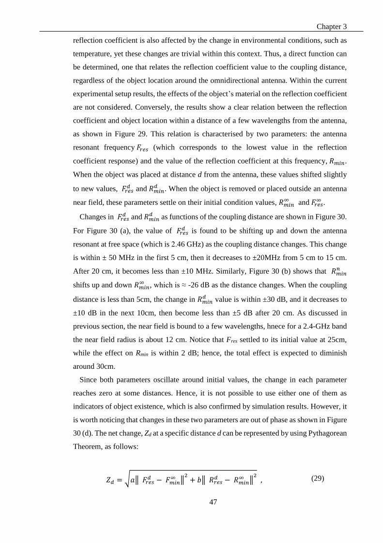
Chapter 3
47
reflection coefficient is also affected by the change in environmental conditions, such as
temperature, yet these changes are trivial within this context. Thus, a direct function can
be determined, one that relates the reflection coefficient value to the coupling distance,
regardless of the object location around the omnidirectional antenna. Within the current
experimental setup results, the effects of the object’s material on the reflection coefficient
are not considered. Conversely, the results show a clear relation between the reflection
coefficient and object location within a distance of a few wavelengths from the antenna,
as shown in Figure 29. This relation is characterised by two parameters: the antenna
resonant frequency 𝐹𝑟𝑒𝑠 (which corresponds to the lowest value in the reflection
coefficient response) and the value of the reflection coefficient at this frequency, 𝑅𝑚𝑖𝑛.
When the object was placed at distance d from the antenna, these values shifted slightly
to new values, 𝐹𝑟𝑒𝑠𝑑 and 𝑅𝑚𝑖𝑛
𝑑 . When the object is removed or placed outside an antenna
near field, these parameters settle on their initial condition values, 𝑅𝑚𝑖𝑛∞ and 𝐹𝑟𝑒𝑠
∞ .
Changes in 𝐹𝑟𝑒𝑠𝑑 and 𝑅𝑚𝑖𝑛
𝑑 as functions of the coupling distance are shown in Figure 30.
For Figure 30 (a), the value of 𝐹𝑟𝑒𝑠𝑑 is found to be shifting up and down the antenna
resonant at free space (which is 2.46 GHz) as the coupling distance changes. This change
is within ± 50 MHz in the first 5 cm, then it decreases to ±20MHz from 5 cm to 15 cm.
After 20 cm, it becomes less than ±10 MHz. Similarly, Figure 30 (b) shows that 𝑅𝑚𝑖𝑛𝑛
shifts up and down 𝑅𝑚𝑖𝑛∞ , which is ≈ -26 dB as the distance changes. When the coupling
distance is less than 5cm, the change in 𝑅𝑚𝑖𝑛𝑑 value is within ±30 dB, and it decreases to
±10 dB in the next 10cm, then become less than ±5 dB after 20 cm. As discussed in
previous section, the near field is bound to a few wavelengths, hnece for a 2.4-GHz band
the near field radius is about 12 cm. Notice that Fres settled to its initial value at 25cm,
while the effect on Rmin is within 2 dB; hence, the total effect is expected to diminish
around 30cm.
Since both parameters oscillate around initial values, the change in each parameter
reaches zero at some distances. Hence, it is not possible to use either one of them as
indicators of object existence, which is also confirmed by simulation results. However, it
is worth noticing that changes in these two parameters are out of phase as shown in Figure
30 (d). The net change, Zd at a specific distance d can be represented by using Pythagorean
Theorem, as follows:
𝑍𝑑 = √𝑎‖ 𝐹𝑟𝑒𝑠
𝑑 − 𝐹𝑚𝑖𝑛∞ ‖
2+ 𝑏‖ 𝑅𝑟𝑒𝑠
𝑑 − 𝑅𝑚𝑖𝑛∞ ‖
2 , (29)

Chapter 3
48
where a and b are generic parameters used to tune the sensitivity of the antenna to 𝐹𝑟𝑒𝑠𝑑
and 𝐹𝑚𝑖𝑛𝑑 . For the current setup, Zd is calculated as
𝑍𝑑 = √0.5 ∗ ‖ 𝐹𝑟𝑒𝑠
𝑑 − 2.48𝐺ℎ𝑧‖2
+ ‖ 𝑅𝑟𝑒𝑠𝑑 − (−25𝑑𝐵)‖
2 . (30)
Figure 30 (d) shows the calculated values of Zd with distance, using (30). Although the
Zd response hasn’t shown a proportional or monotonic relation with distance, the response
can be divided into three distinct regions: (a) Zd > 20 in the first 3cm, (b) 3<Zd <13
between 5cm and 15cm, and (c) Zd <5 approximately, for distances larger than 13cm.
Therefore, Zd gives an approximate indication of object existence with a dipole antenna
near-field area.
Figure 30: Change with distance: (a) Fres vs distance, (b) Rmin vs distance, (c) Fres vs
Rmin and (d) Zd vs distance
0 5 10 15 20 250
5
10
15
20
25
30
35
40
Distance (cm)
Zd
0 5 10 15 20 252.4
2.42
2.44
2.46
2.48
2.5
2.52
Distances (cm)
Fre
s (
GH
z)
0 5 10 15 20 25-50
-45
-40
-35
-30
-25
-20
-15
-10
-5
Distances (cm)
Rm
in (d
B)
(a) (b)
(d)
-60 -50 -40 -30 -20 -10 02.44
2.45
2.46
2.47
2.48
2.49
2.5
Rmin
(dB)
Fre
s (
GH
z) 5 cm
6 cm
7 cm
8 cm
9 cm
10 cm
11 cm
12 cm
(c)
Chapter 3
49
3.4 Object Location Classification Using Principal Component Analysis
From the previous section, it was concluded that it is possible to specify the
approximate distance between an antenna and a metallic object placed within the near
field, based on the antenna reflection coefficient. In this section, another step was taken
to classify the object location with respect to the LOS between two communicating
antennas, using principal component analysis (PCA). The classifier was applied to
distinguish between the measurements from the three positions shown in Figure 19. The
classifier uses the reflection coefficient response (magnitude and phase), as well as the
transmission coefficient (magnitude and phase).
In the subsections below, a brief description of the PCA method is presented, then the
classification approaches and results are discussed in detail. In the third section a study
of the results statistical significance is presented.
3.4.1 Principal Component Analysis (PCA) Classifier
Principal Component Analysis (PCA) provides an advanced mathematical procedure
to analyse data in multi-dimensional variable space and reflect data into lower
dimensional space. It is mathematically defined as an orthogonal linear
transformation that transforms the data to a new coordinate system such that the greatest
variance by some projection of the data comes to lie on the first coordinate (called the
first principal component), the second greatest variance lies on the second coordinate and
so on. A simplified background on the method and the used MATLAB code are presented
in Appendix A. For more details on the PCA classification, a quick tutorial is presented
in [106], while [107] provides an extensive guide of the method and its applications.
3.4.2 Classification Methodology and Results
To apply the PCA, the data should be arranged in an n × m matrix, where n is the
number of observations and m is the number of variables. The analysis in this section uses
the experimental measurements obtained in Section 3.2. The PCA classifier was applied
twice, each time with a different approach, depending on the way the data was organised.
The results of the two approaches are shown in Figure 31 and Figure 32.
In the first approach, the experimental measurements were arranged as 79
measurements (observations). The first 75 observations represents measurements for the
75 locations in the experiment, which are based recorded at 3 positions: p1, p2 and p3. At
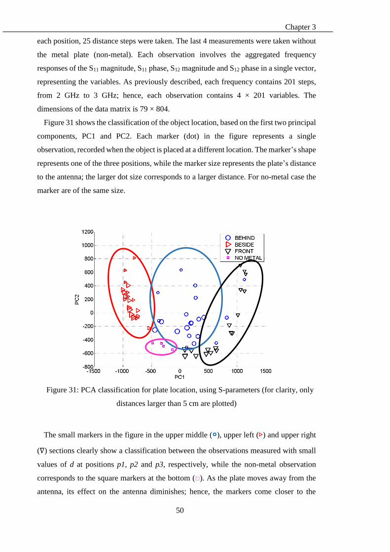
Chapter 3
50
each position, 25 distance steps were taken. The last 4 measurements were taken without
the metal plate (non-metal). Each observation involves the aggregated frequency
responses of the S11 magnitude, S11 phase, S12 magnitude and S12 phase in a single vector,
representing the variables. As previously described, each frequency contains 201 steps,
from 2 GHz to 3 GHz; hence, each observation contains 4 × 201 variables. The
dimensions of the data matrix is 79 × 804.
Figure 31 shows the classification of the object location, based on the first two principal
components, PC1 and PC2. Each marker (dot) in the figure represents a single
observation, recorded when the object is placed at a different location. The marker’s shape
represents one of the three positions, while the marker size represents the plate’s distance
to the antenna; the larger dot size corresponds to a larger distance. For no-metal case the
marker are of the same size.
Figure 31: PCA classification for plate location, using S-parameters (for clarity, only
distances larger than 5 cm are plotted)
The small markers in the figure in the upper middle (∘), upper left (▷) and upper right
(∇) sections clearly show a classification between the observations measured with small
values of d at positions p1, p2 and p3, respectively, while the non-metal observation
corresponds to the square markers at the bottom (□). As the plate moves away from the
antenna, its effect on the antenna diminishes; hence, the markers come closer to the

Chapter 3
51
regions that represent the non-metal case. For large values of d, all of the markers settle
on the bottom, and the classifier is unable to be clearly distinguished between the
observations.
Since the PCA is a feature selection method, a second approach for classification was
implemented using selected features of the same data sets. The responses of S11 and S12
were processed to produce five features, as listed in Table 3. The five features were
calculated for each distance step and position in the previous setup. Hence, the dimension
of the data matrix to be classified was 79 × 5, where each feature represents a variable.
The aim of this approach is to find the features are most effective to be used as indicator
for the object location and distance. However, the observations of position p1 and p3 are
not clearly classified in this approach. Figure 32 shows the results of using PCA with the
selected features. It can be seen that Features 3 and 5 are better than the other features in
terms of distinguishing between the results (other features are appearing closer to the
figure’s origin, and their labels were removed for clarity).
Table 3: Features and their calculations
Feature name Feature Calculation
Feature 1 Mean value of S12 magnitude response
Feature 2 Mean value of S12 phase response
Feature 3 𝑅𝑚𝑖𝑛
Feature 4 𝐹𝑟𝑒𝑠
Feature 5 Peak-to-peak of S11 phase response
In conclusion, Figure 31 shows that the PCA method have the potential to distinguish
between different changes in antenna measurements due to different object locations
around the antenna, while Figure 32 shows that among the proposed features, antenna
return loss and Peak-to-peak of S11 phase are the most useful to detect the object location
and distance.
To quantity the group classification showed in Figure 31, the results should be proven
statistically significant. One way to prove that is by calculating the F-ratio of observed
data (sample data set) and compare it to the f-distribution of the population data set. Since
the population data set is unknown, its distribution can be approximated by statistical
methods such as Bootstrap method and permutation test [108]. The statistical significance
of the results is presented in the next section.

Chapter 3
52
3.4.3 Statistical Significance of PCA Results
This section present the statistical significance calculation using permutation test.
Permutation tests are used for nonparametric hypothesis testing. The objective of
permutation tests is to determine whether an observed statistic deviates significantly from
its null distribution, which is established conditionally on the data, and does not require a
particular probability model. This characteristic of the permutation procedure matches the
nonparametric nature of PCA, which makes the procedure suitable for inference in PCA.
To establish a null distribution, first, the correlational structure of the observed data is
destroyed by randomly rearranging the values within each variable (independent of the
other variables). In this way, a data matrix of the same size as the original data matrix is
constructed, with a random structure [108].
The statistical significance calculation on the PCA results shown in fig are explained
in the next steps:
1. Define the null hypothesis:
𝐻0: 𝜇𝑓𝑟𝑜𝑛𝑡 = 𝜇𝑏𝑒𝑠𝑖𝑑𝑒 = 𝜇𝑏𝑒ℎ𝑖𝑛𝑑 = 𝜇𝑛𝑜 𝑚𝑒𝑡𝑎𝑙 , (31)
or in other word: PC1 and PC2 do not distinguish between the different
observations.
2. Specify the level of significance (α): Here it was set to the default value 0.05.
3. Select suitable number to repeat the permutation process:
The minimum number of permutation is related to the significance level as follow:
𝑚𝑖𝑛𝑝𝑒𝑟𝑚 =
1
𝛼=
1
0.05= 20. (32)
The maximum number of permutation is bounded by the number of possible
ways to rearrange the observations while keeping the same number of groups and
the same number of elements in each group. It is calculated as follow:
𝑚𝑎𝑥𝑝𝑒𝑟𝑚 =
(𝑛1 + 𝑛2 + … + 𝑛𝑛)!
𝑛1! 𝑛2! … 𝑛𝑛! , (33)

Chapter 3
53
where n1, n2, … are the number of observations in each group. In the setup
explained in the previous section the results belong to four groups that contain 25,
25, 25 and 4 observations respectively. Therefore the maximum number of
possible permutation calculated as follow:
𝑚𝑎𝑥𝑝𝑒𝑟𝑚 =
79!
25! 25! 25! 4! . (34)
However this number is tremendously large and usually a much less number of
permutations is enough for the purpose of statistical significance calculation. As
suggested by [109], permutation number should be larger than 99, because
permutation tests with a smaller number of permutations than 99 have too little
power. Here we select the number of permutation to be 10000.
4. Generate the permutated data sets:
It should be noted that since the variables in this test have different value ranges
and means, the permutation is done only within columns. Also, each new
permutated data set was compared to previously generated data sets to avoid the
repetition.
5. Calculate the F-ratio for each permutation:
The F-ratio is defined as the ratio of the between-group variability to the within-
group variability, and it is calculated as follow:
𝐹𝑟𝑎𝑡𝑖𝑜 =
∑ 𝑛𝑖(�̅�𝑖 − �̅�)2𝑘𝑖=1
𝑘 − 1
∑ ∑ (𝑥𝑖𝑗 − �̅�𝑖)2𝑛𝑖
𝑗=1𝑘𝑖=1
𝑛 − 𝑘
, (35)
where:
k is the number of groups,
ni is the number of observations in the ith group,
xij is the jth observation of the ith group,
�̅� is the mean of all observations,
�̅�𝑖 is the mean of observations in the ith group.
Since there are two principal components (PC1 and PC2), F-ratio is calculated for
each component and the maximum value between the two is considered for the
next steps.

Chapter 3
54
6. Generate the F-distribution of the population set by aggregate the F-ratio values
from all the permutation.
7. Calculate the F-ratio for the observed data set (original data set).
8. Calculate Fc, which is defined as the number of permutations with F-ratio larger
than the F-ratio of the original data set.
9. Calculate the p-value as follow:
𝑝𝑣𝑎𝑙𝑢𝑒 =
𝑛𝑜. 𝑜𝑓 𝑃𝑒𝑟𝑚𝑢𝑎𝑡𝑖𝑜𝑛 − 𝐹𝑐
𝑛𝑜. 𝑜𝑓 𝑃𝑒𝑟𝑚𝑢𝑎𝑡𝑖𝑜𝑛 . (36)
The calculation were performed using MATLAB code listed in the next section. The
calculated p-values are 1*10-5 and 0.0406 for the first and second principal component,
respectively. Both of the p-values are below the selected level of significance, hence, we
reject the null hypothesis.
Finally it is worth to notice two implications in the calculated p-values:
As expected, the p-value of the first principal component is larger than the p-
value of the second component, because the PCA algorithm sort the component
based on their eigenvalues.
To apply the permutation test, the observations in each groups assumed to be
independent and identically distributed random variables. However, this is true
only for the fourth group were the measurement repeated four times without the
metallic plate. For each one of the other three groups, the test were repeated 25
times with changing the distance to the metallic plate at each time. It likely to get
a better classification result (lower p-values) if the measurements were repeated
without changing the distance.
3.5 Metallic Object Near Two Adjacent Antennas – Experiment II
In this section, the effect of a metallic object on the received power interference of two
adjacent antennas was studied. Although distance measurements using frequency
sweeping is a well-researched area [110, 111], this section investigates the ability of a
low profile antenna, commercially available for current WSN technology, to be used as a
detector for a nearby metallic object. Distance measurement using frequency sweeping is

Chapter 3
55
an interesting technique, and it depends only on the received signal magnitude, making it
suitable for inexpensive, off-the-shelf transceiver circuits. Also, it isn’t affected by the
fading caused by power losses over distance, as this techniques depends on the changes
in the signal across frequency range rather than on the signal’s absolute value. However,
in our experimental setup, the reflection effect upon the metal plate was found to be too
weak for distances further than 1 m, as it vanished rapidly.
Figure 32: PCA classification for plate location, using extracted features of
S-parameters
Figure 33: Distance measurement using two adjacent nodes
The experiment was conducted inside the same anechoic chamber described in
Section 3.2. Two 2.4-GHz dipole antennas were fixed 10 cm apart and connected to an
Reflected signal
Transmitted signal
Metallic
plate
Two dipole
antennas
Network Analyser

Chapter 3
56
Agilent-8363B Network Analyser. Both antennas were placed vertically, facing a metal
plate (30 cm × 20 cm), which is fixed, using a sample holder that moves on a 1-m ramp.
The distance (d) between the plate and the antennas was increased from 5 cm to 100 cm
with 1 cm steps. At each step, the received signal is recorded over the frequency range,
from 2 GHz to 3 GHz, with 5 MHz steps. Existence of other objects, i.e., the wooden
ramp, desks and plastic holder, will affect the reading; however, the change in the signal
will be related only to the metal plate, as it is the only thing that can change its position
at each distance step.
By aggregating the S12 response for each distance step, a 2D surface for Vrec(d,f), as a
function of distance and frequency, is formulated. Figure 34 (a) shows the surface
produced experimentally, while Figure 34 (b) shows similar results calculated
analytically, using the reflection model in Section 2.2.3 for the same frequency and
distance steps.
Figure 34: Vrec(d,f) surface: (a) experimental and (b) simulation
The white regions in the figures represent peaks of the standing wave, while the dark
regions represent the valleys. It should be noted that, to achieve this graph, the following
steps were taken:
1. Vrec values represent the square root for the absolute magnitude of the S12 response.
2. Vrec values were normalised to the antenna pattern over a distance, to cancel the
effect of fading due to distance change; i.e., at each distance step, the Vrec response
over frequency was normalised to its mean value.
3. Then Vrec values were normalised to the antenna gain distribution across the
frequency range. (Since the antenna gain is higher at the antenna resonant
frequency).
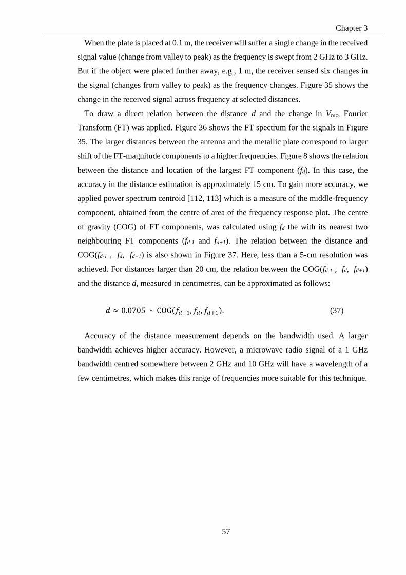
Chapter 3
57
When the plate is placed at 0.1 m, the receiver will suffer a single change in the received
signal value (change from valley to peak) as the frequency is swept from 2 GHz to 3 GHz.
But if the object were placed further away, e.g., 1 m, the receiver sensed six changes in
the signal (changes from valley to peak) as the frequency changes. Figure 35 shows the
change in the received signal across frequency at selected distances.
To draw a direct relation between the distance d and the change in Vrec, Fourier
Transform (FT) was applied. Figure 36 shows the FT spectrum for the signals in Figure
35. The larger distances between the antenna and the metallic plate correspond to larger
shift of the FT-magnitude components to a higher frequencies. Figure 8 shows the relation
between the distance and location of the largest FT component (fd). In this case, the
accuracy in the distance estimation is approximately 15 cm. To gain more accuracy, we
applied power spectrum centroid [112, 113] which is a measure of the middle-frequency
component, obtained from the centre of area of the frequency response plot. The centre
of gravity (COG) of FT components, was calculated using fd the with its nearest two
neighbouring FT components (fd-1 and fd+1). The relation between the distance and
COG(fd-1 , fd, fd+1) is also shown in Figure 37. Here, less than a 5-cm resolution was
achieved. For distances larger than 20 cm, the relation between the COG(fd-1 , fd, fd+1)
and the distance d, measured in centimetres, can be approximated as follows:
𝑑 ≈ 0.0705 ∗ COG(𝑓𝑑−1, 𝑓𝑑 , 𝑓𝑑+1). (37)
Accuracy of the distance measurement depends on the bandwidth used. A larger
bandwidth achieves higher accuracy. However, a microwave radio signal of a 1 GHz
bandwidth centred somewhere between 2 GHz and 10 GHz will have a wavelength of a
few centimetres, which makes this range of frequencies more suitable for this technique.

Chapter 3
58
Figure 35: Vrec(d,f) at selected distances
Figure 36: Fourier Transform of signal in Figure 35: (a) 1 cm, (b) 50 cm and
(c) 100 cm, (Only the first 20 components are shown, as the rest are very close to zero).
Vre
c
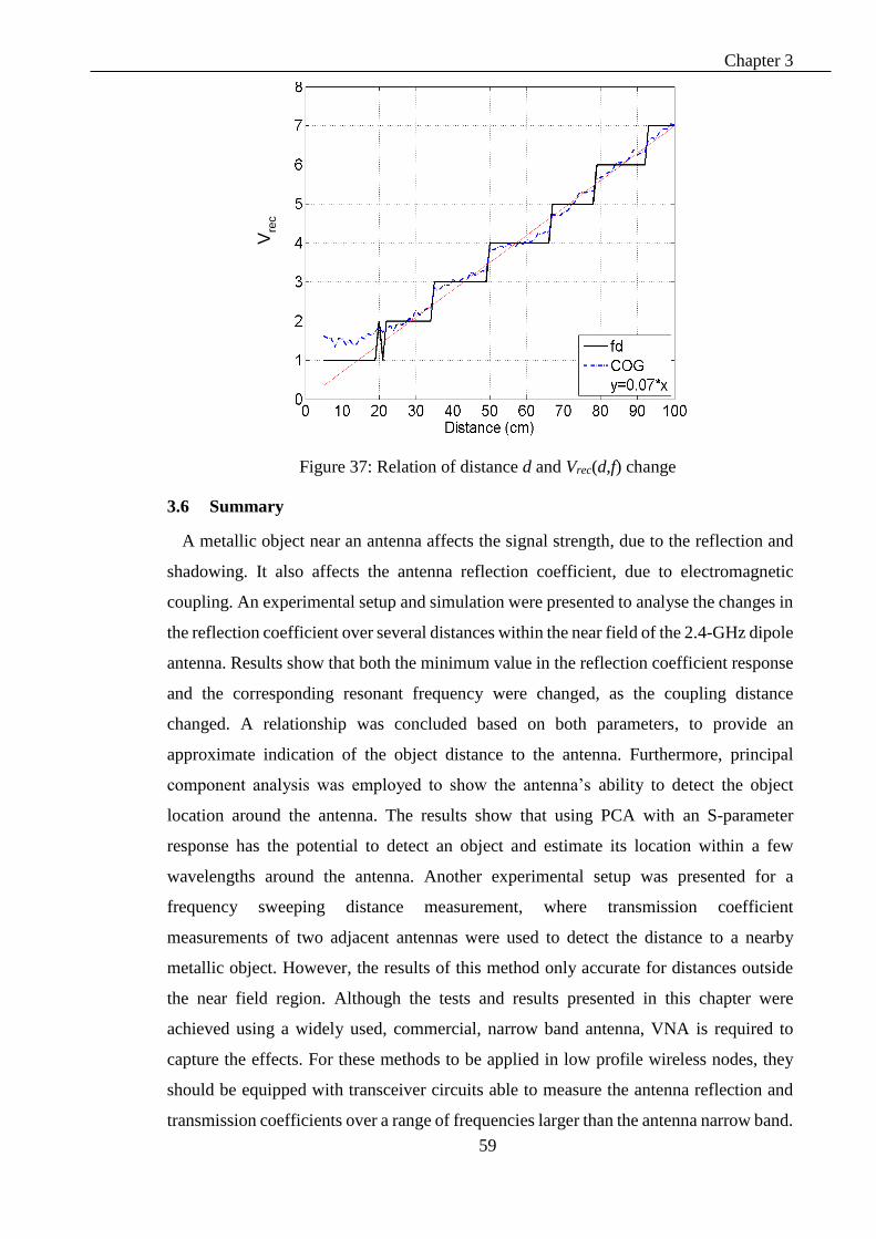
Chapter 3
59
Figure 37: Relation of distance d and Vrec(d,f) change
3.6 Summary
A metallic object near an antenna affects the signal strength, due to the reflection and
shadowing. It also affects the antenna reflection coefficient, due to electromagnetic
coupling. An experimental setup and simulation were presented to analyse the changes in
the reflection coefficient over several distances within the near field of the 2.4-GHz dipole
antenna. Results show that both the minimum value in the reflection coefficient response
and the corresponding resonant frequency were changed, as the coupling distance
changed. A relationship was concluded based on both parameters, to provide an
approximate indication of the object distance to the antenna. Furthermore, principal
component analysis was employed to show the antenna’s ability to detect the object
location around the antenna. The results show that using PCA with an S-parameter
response has the potential to detect an object and estimate its location within a few
wavelengths around the antenna. Another experimental setup was presented for a
frequency sweeping distance measurement, where transmission coefficient
measurements of two adjacent antennas were used to detect the distance to a nearby
metallic object. However, the results of this method only accurate for distances outside
the near field region. Although the tests and results presented in this chapter were
achieved using a widely used, commercial, narrow band antenna, VNA is required to
capture the effects. For these methods to be applied in low profile wireless nodes, they
should be equipped with transceiver circuits able to measure the antenna reflection and
transmission coefficients over a range of frequencies larger than the antenna narrow band.
Vre
c
60
Chapter 4 DESIGN AND IMPLEMENTATION OF
A LOW SENSITIVITY UWB ANTENNA FOR
WBAN APPLICATIONS

Chapter 4
61
4.1 Chapter Outline
In the framework of near field sensing in body area network, this chapter presents a
new design for the UWB WBAN antenna. The chapter aims to introduce a design that
conforms to the WBAN requirements of size, while achieving very low sensitivity when
it comes in contact with the human body. As discussed in Chapter 2, the WBAN antenna
is required to have an almost uniform radiation pattern in the plane parallel to the human
body, and the radiation towards the body should be minimised to reduce absorption by
the body tissue. The design starts by choosing a Vivaldi antenna widely used for ultra-
wide band (UWB) application. Parametric studies and optimisation are presented at
several design stages to maintain the reflection coefficient and radiation pattern within
the WBAN requirements. Both the curved reflector and the horizontal feeding enhance
the placement on the human body, while preserving a simple structure. Figure 38 shows
the work flowchart.
This chapter is organised as follows. Section 4.2 introduces a brief background on the
UWB WBAN requirement and related work. The design concept and simulation results
are presented in Section 4.3, while the design implementation and experimental results
are presented in Section 4.4. The tests of the antenna on the human body are discussed
in 4.5. Finally, Section 4.6 concludes the chapter.
4.2 Background
A wide variety of applications that benefit from a wireless body area network (WBAN)
requires both robust communications and high-precision ranging capabilities. These
applications spans form the medical field to entertainment and gaming areas. Therefore,
there has been an increasing interest in recent years in the use of ultra-wide-band (UWB)
transmission technology in WBAN to fulfil these requirements. Low energy, spectral
density, and the simplicity of the transceiver architecture are the main features that make
UWB technology a good candidate for WBAN applications. Moreover, a UWB impulse
radio can be used for robust data communications and precision ranging due its low
susceptibility to multipath fading [114]. The desired operating frequencies for UWB are
defined by U.S. Federal Communications Commission (FCC) regulations as 3.1 to 10.6
GHz.
One of the main challenges of a UWB system is the antenna design, as it plays a critical
role in the WBAN applications. Generally, the UWB antennas require a compact form
and low height, in addition to other inherent requirements, such as low back radiation and

Chapter 4
62
suitable transient characteristics. However, reducing the UWB antenna size usually
comes at the expense of deforming the radiation pattern and/or reducing the frequency
bandwidth, due to impedance mismatch.
Figure 38: Flowchart of this chapter
Studies of the effects on antenna characteristics due to the human body and passive
objects placed within the antenna near field have been increasing with the increase of
wireless mobile devices [115-117]. Among the many designs for WBAN UWB antennas
in previous studies, several have achieved reduced antenna dimensions, while
maintaining good radiation and impedance measurements [5-8, 118]. Chahat [8] proposed
a small printed UWB antenna with an overall height of 10 mm. The antenna showed good
impedance matching over a UWB frequency range. A novel antenna presented by [5]
consists of a bevel-edge feed structure and a metal plate with a folded strip, totalling 10
mm in height. The antenna shows a directional pattern with low back radiation, due to the
50 × 50 mm2 ground plane. A directional, reduced-size wide slot antenna was presented
by [118] for the 6-10 GHz band. A reflector plate was added to block the back radiation,
making the final antenna height around 7 mm. Another low profile antenna, 8.5 mm in
Par
amet
ric
study
Opti
miz
atio
n

Chapter 4
63
height, was presented by [6] for WBAN. The antenna consists of two parts: a central
mono-cone, responsible for the high frequency band, and a top-cross-plate, responsible
for the lower frequency band. Both are fixed on a reflection plate that is 50 × 50 mm2.
The 3D printed miniaturised UWB antenna designed by [7] covers a wide frequency
range, from 3.5-29.8 GHz. The design is characterised by its very small length and width
dimensions compared to other designs, yet its height is 15 mm. It is worth noting that,
although these designs offer an antenna height that is less than 15 mm [6-8], they require
a vertical feeding (normal to the human body), which adds to the antenna height when it
is installed on the human body and in the clothes.
Alternatively, a Vivaldi antenna is one of the promising candidates for UWB
communication, due to its simple structure, broad band and high directionality. The
Vivaldi design was first proposed by [119] and it has been adapted later by many
researchers for several applications [120-122]. However, to accommodate a lower
frequency, the antenna tend to have larger dimensions relative to other types of printed
antennas. Several researchers have tackled Vivaldi antenna miniaturisation by
introducing a loading element [123], slot edge [124], or stepped structure [125] to the
original Vivaldi shape. However it is uncommon to use Vivaldi design in wearable
applications because the antenna boresight extends along its length, making the antenna
unsuitable for WBAN requirements. As an example, a new antenna design was proposed
for on-body communication with an implanted capsule was presented by Wang [126]. In
his design, a Vivaldi antenna was adopted to establish effective and efficient wireless
links with the implanted capsule. The design is composed of four elements antenna on
single substrate. Each element is composed of two opposite Vivaldi variants on one side
of the substrate and is fed by a radial stub microstrip on the other side. With a metallic
reflector at the Vivaldi side, a strong broadside radiation can be obtained from two
opposite end-fire radiations resulting from two opposite planar Vivaldi variants. The final
dimensions of the design are 131×131×10 mm3. Results shows that 15-25 dB decoupling
between the co- and cross-polarized components can be observed in 3-10 GHz.
4.3 Antenna Design Concept and Performance
The Vivaldi antenna is characterised by its high-gain, simple structure. However, the
antenna is also known for its high directionality along it longest dimension. To comply
with WBAN requirements, two Vivaldi antennas were placed on a single chip; by
combining two opposite Vivaldi antennas on one PCB, the design achieves a more diverse
radiation pattern in the PCB plane.
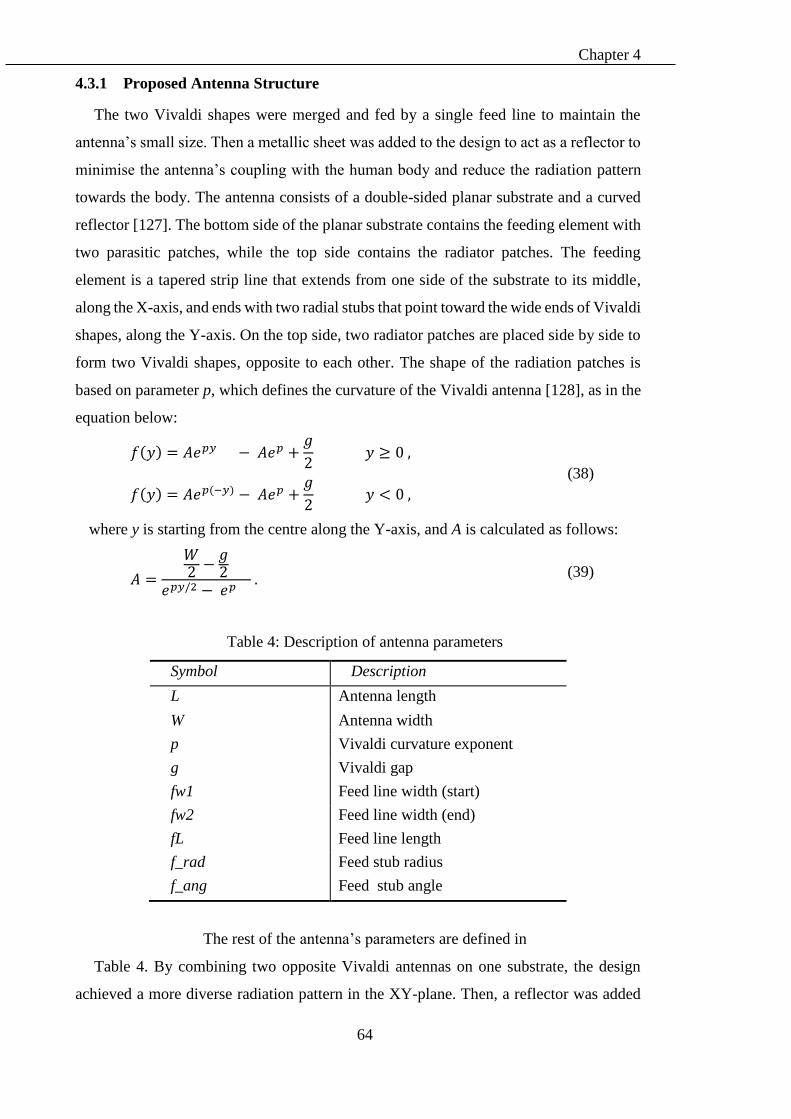
Chapter 4
64
4.3.1 Proposed Antenna Structure
The two Vivaldi shapes were merged and fed by a single feed line to maintain the
antenna’s small size. Then a metallic sheet was added to the design to act as a reflector to
minimise the antenna’s coupling with the human body and reduce the radiation pattern
towards the body. The antenna consists of a double-sided planar substrate and a curved
reflector [127]. The bottom side of the planar substrate contains the feeding element with
two parasitic patches, while the top side contains the radiator patches. The feeding
element is a tapered strip line that extends from one side of the substrate to its middle,
along the X-axis, and ends with two radial stubs that point toward the wide ends of Vivaldi
shapes, along the Y-axis. On the top side, two radiator patches are placed side by side to
form two Vivaldi shapes, opposite to each other. The shape of the radiation patches is
based on parameter p, which defines the curvature of the Vivaldi antenna [128], as in the
equation below:
𝑓(𝑦) = 𝐴𝑒𝑝𝑦 − 𝐴𝑒𝑝 +𝑔
2 𝑦 ≥ 0 ,
𝑓(𝑦) = 𝐴𝑒𝑝(−𝑦) − 𝐴𝑒𝑝 +𝑔
2 𝑦 < 0 ,
(38)
where y is starting from the centre along the Y-axis, and A is calculated as follows:
𝐴 =
𝑊2 −
𝑔2
𝑒𝑝𝑦/2 − 𝑒𝑝 . (39)
Table 4: Description of antenna parameters
Symbol Description
L Antenna length
W Antenna width
p Vivaldi curvature exponent
g Vivaldi gap
fw1 Feed line width (start)
fw2 Feed line width (end)
fL Feed line length
f_rad Feed stub radius
f_ang Feed stub angle
The rest of the antenna’s parameters are defined in
Table 4. By combining two opposite Vivaldi antennas on one substrate, the design
achieved a more diverse radiation pattern in the XY-plane. Then, a reflector was added

Chapter 4
65
to enhance the front radiation (along the +Z axis) and to reduce the radiation in the back
hemisphere (along the -Z axis). The feeding point was connected to the strip line and one
of the radiator patches. The schematic diagram of the top and bottom sides of the patch is
shown in Figure 39 (a) and Figure 39 (b), respectively, while Figure 39 (c) shows the
relative position of the reflector. Figure 40 shows a perspective view of the design.
Figure 39: Antenna schematic: (a) bottom side, (b) top side and (c) reflector position
Figure 40: Proposed antenna (perspective view)

Chapter 4
66
4.3.2 Parametric Study and Optimization
A parametric study was performed using selected parameters (shown in Table 5). The
aim of the parametric study was to find the values that achieve the best impedance
matching for the antenna, with a reflection coefficient of less than -10dB on the
majority of the specified frequency band. Among the 216 simulation runs, only a few
value combinations achieved this goal. Figure 41 shows seven selected responses that
achieved -10dB over most of the UWB frequency range. The corresponding parameters
of these seven simulation runs are listed in
Table 6. Generally, the width of the Vivaldi antenna should be greater than or equal to
half the wavelength of the lower frequencies. However, results showed that changing the
antenna width and length within the selected ranges doesn’t have a significant effect on
the impedance matching. The best values are shown to occur when the exponent, p, is set
to a low value (around 0.2 mm), the feed line width is 3 mm and the feed line length is
longer than half the antenna width.
Finally, the design parameters were optimised using the ‘Trust Region Framework’
optimisation method provided by CST MWS software. All of the parameters listed in
Table 4 were optimised to within 10% of their initial values. The domain accuracy of
the optimisation method was set to 0.001. The final values of the optimisation process are
listed in Table 7.
Table 5: Parametric study instances
Parameter Parametric instances
L 40, 52, 64 mm
W 48, 49, 50 mm
fW1 1, 2, 3 mm
fL 24, 25, 26 mm
p 0.2, 0.5, 0.7 mm
g 1.6, 2, 2.4 mm
f_ang 90°, 120°, 150°
Table 6: Parameter values for the responses shown in Figure 3
Run ID W L p g fw1 fL f_ang
1 48.0 26.0 0.2 1.6 3.0 26.0 120°
2 48.0 26.0 0.2 2.0 3.0 26.0 120°
3 49.0 26.0 0.2 2.0 3.0 26.0 120°
4 50.0 26.0 0.2 2.0 3.0 26.0 120°
5 48.0 26.0 0.2 2.4 3.0 26.0 120°
6 49.0 26.0 0.2 2.4 3.0 26.0 120°
7 48.0 32.0 0.2 2.4 3.0 26.0 120°

Chapter 4
67
Table 7: Antenna parameters (mm) after optimisation
L W L1 W1 p g fw1 fw2 fL rad
52 48 21.4 21.9 0.23 2.8 3.2 1.8 26.7 117°
Figure 41: Reflection coefficient response for selected cases in the parametric study
instances
4.3.3 Reflector Effect and Reflector Parametric Study
Although the Vivaldi antenna is a very good directional antenna, in the proposed
design, both Vivaldi shapes are aligned to the body surface. To enhance the radiation
pattern along the Z-axis, a reflector was added. Other ways to achieve a directional
antenna pattern include adding the cavity or shielding plane behind the antenna or using
the absorbing materials [129]. The usage a reflector with a WBAN antenna not only
minimises the effects of the human body’s proximity and body exposure to EM radiation,
but it also increases the front lobe radiation, compared to the other methods. However,
the introduction of a reflecting element had a large effect on the input impedance of the
antenna, especially when the antenna is not inherently directional [58, 130, 131].
The proposed reflector, made of a thin copper sheet, is placed behind the substrate
facing the bottom side, and the sheet is bent in an elliptical curve. Figure 39 (c) shows the

Chapter 4
68
relative position of the reflector. The major radius is fixed at L/2, where L is the antenna
length, while the minor radius, br, is variable. Hence, the sheet width is equal to the
substrate width, and is slightly longer than the substrate to compensate for the curvature.
The distance between the PCB and the reflector centre, dr, equals 5mm. To evaluate the
reflector effect on antenna performance, a comparison of the antenna measurements
without a reflector, with a flat reflector and with a curved reflector (shown in Figure 42)
is conducted in terms of the radiation pattern and reflection coefficient. Figure 43 (a)
shows that the front-to-back ratio on the XY-plane at 4 GHz changes from 0dB to 10 dB
when a flat reflector is added at dr=5 mm. The results show that the change in the radiation
pattern comes at the expense of increasing the reflection coefficient magnitude value
(|S11|). When the reflector is added, there is an increase of about 7 dB in |S11|, as shown
in Figure 43 (b). The total front-to-back ratio for the three selected frequencies at 4 GHz,
7 GHz and 10 GHz are 10.01 dB, 4.37 dB and 5.46 dB, respectively. The total front-to-
back ratio (RTotal), is defined as the ratio of the summation of the radiated power in the
upper hemisphere to the summation of the radiated power in the lower hemisphere, and
is calculated as follow:
𝑅𝑇𝑜𝑡𝑎𝑙 =∑ 𝑃𝑟−90=<𝑡ℎ𝑒𝑡𝑎=<90
∑ 𝑃𝑟𝑡ℎ𝑒𝑡𝑎>90 , 𝑡ℎ𝑒𝑡𝑎<−90 , (40)
Figure 42: Proposed antenna: (a) without a reflector; (b) with a flat reflector; and (c)
with a curved reflector
Figure 43 shows that the curved reflector (with br=5 mm and dr=5 mm) has
(a) (b) (c)

Chapter 4
69
approximately the same effect on the radiation pattern but a lesser effect on the |S11|
compared to the flat reflector. Hence, a curved reflector was adopted for the proposed
antenna design. In addition to the enhancement in the radiation pattern, a curved reflector
is more suitable t mount on human body parts, like an arm or torso, compared to the flat
reflector.
Figure 43: Comparison of the reflector effects, without the parasitic elements: (a) XZ
radiation pattern at 4 GHz and (b) |S11| response
(a)
(b)
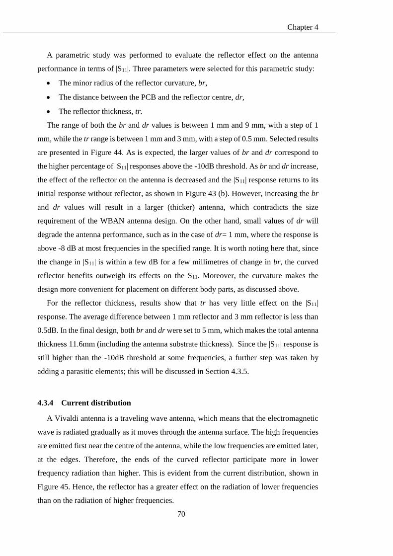
Chapter 4
70
A parametric study was performed to evaluate the reflector effect on the antenna
performance in terms of |S11|. Three parameters were selected for this parametric study:
The minor radius of the reflector curvature, br,
The distance between the PCB and the reflector centre, dr,
The reflector thickness, tr.
The range of both the br and dr values is between 1 mm and 9 mm, with a step of 1
mm, while the tr range is between 1 mm and 3 mm, with a step of 0.5 mm. Selected results
are presented in Figure 44. As is expected, the larger values of br and dr correspond to
the higher percentage of |S11| responses above the -10dB threshold. As br and dr increase,
the effect of the reflector on the antenna is decreased and the |S11| response returns to its
initial response without reflector, as shown in Figure 43 (b). However, increasing the br
and dr values will result in a larger (thicker) antenna, which contradicts the size
requirement of the WBAN antenna design. On the other hand, small values of dr will
degrade the antenna performance, such as in the case of dr= 1 mm, where the response is
above -8 dB at most frequencies in the specified range. It is worth noting here that, since
the change in |S11| is within a few dB for a few millimetres of change in br, the curved
reflector benefits outweigh its effects on the S11. Moreover, the curvature makes the
design more convenient for placement on different body parts, as discussed above.
For the reflector thickness, results show that tr has very little effect on the |S11|
response. The average difference between 1 mm reflector and 3 mm reflector is less than
0.5dB. In the final design, both br and dr were set to 5 mm, which makes the total antenna
thickness 11.6mm (including the antenna substrate thickness). Since the |S11| response is
still higher than the -10dB threshold at some frequencies, a further step was taken by
adding a parasitic elements; this will be discussed in Section 4.3.5.
4.3.4 Current distribution
A Vivaldi antenna is a traveling wave antenna, which means that the electromagnetic
wave is radiated gradually as it moves through the antenna surface. The high frequencies
are emitted first near the centre of the antenna, while the low frequencies are emitted later,
at the edges. Therefore, the ends of the curved reflector participate more in lower
frequency radiation than higher. This is evident from the current distribution, shown in
Figure 45. Hence, the reflector has a greater effect on the radiation of lower frequencies
than on the radiation of higher frequencies.
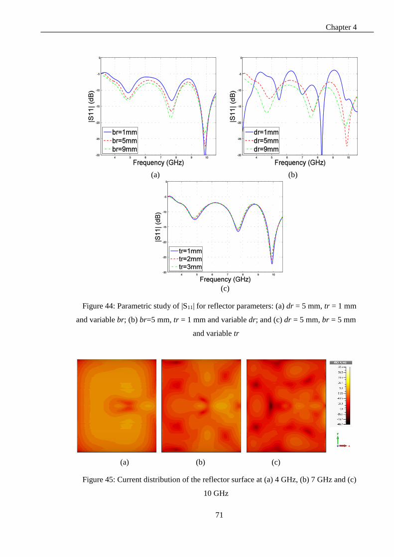
Chapter 4
71
Figure 44: Parametric study of |S11| for reflector parameters: (a) dr = 5 mm, tr = 1 mm
and variable br; (b) br=5 mm, tr = 1 mm and variable dr; and (c) dr = 5 mm, br = 5 mm
and variable tr
Figure 45: Current distribution of the reflector surface at (a) 4 GHz, (b) 7 GHz and (c)
10 GHz
(a) (b)
(c)
(b) (c) (a)
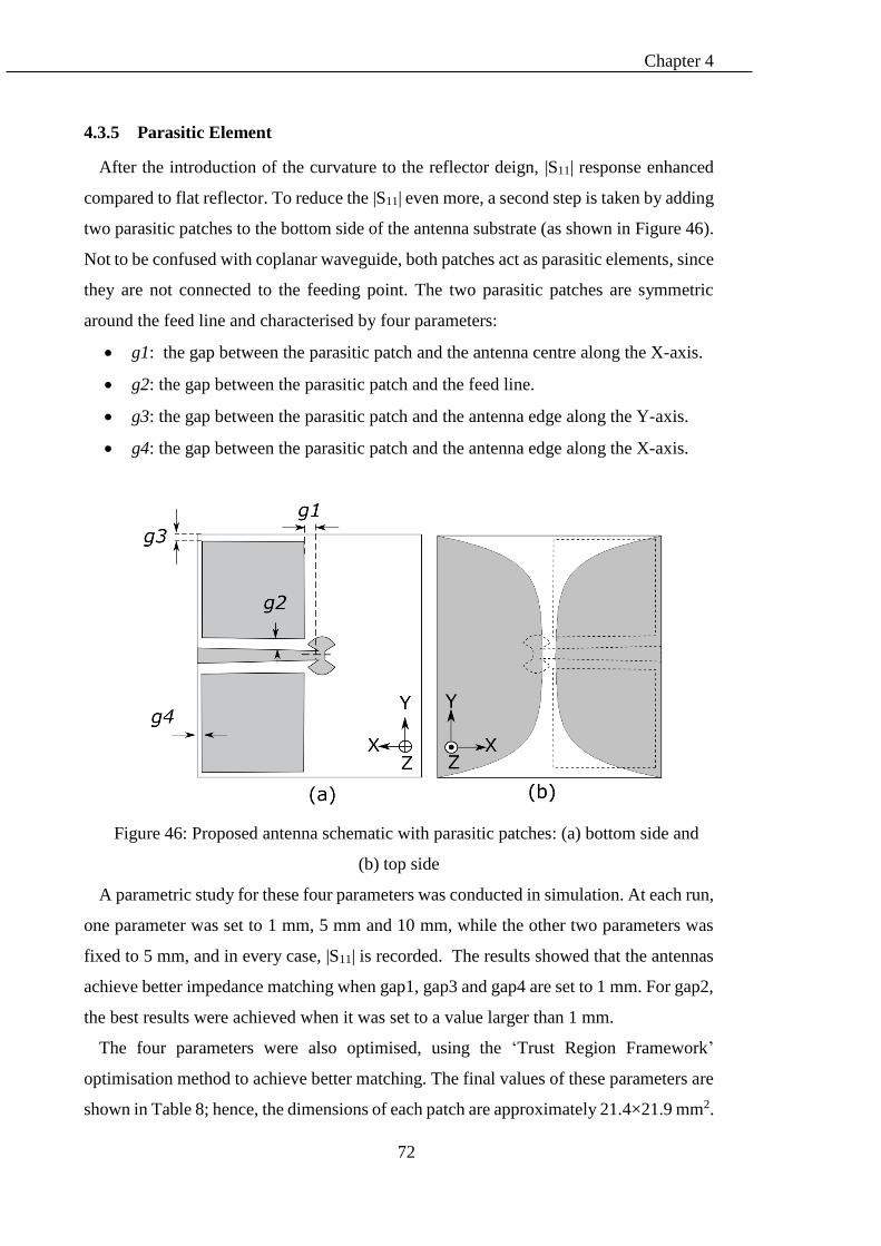
Chapter 4
72
4.3.5 Parasitic Element
After the introduction of the curvature to the reflector deign, |S11| response enhanced
compared to flat reflector. To reduce the |S11| even more, a second step is taken by adding
two parasitic patches to the bottom side of the antenna substrate (as shown in Figure 46).
Not to be confused with coplanar waveguide, both patches act as parasitic elements, since
they are not connected to the feeding point. The two parasitic patches are symmetric
around the feed line and characterised by four parameters:
g1: the gap between the parasitic patch and the antenna centre along the X-axis.
g2: the gap between the parasitic patch and the feed line.
g3: the gap between the parasitic patch and the antenna edge along the Y-axis.
g4: the gap between the parasitic patch and the antenna edge along the X-axis.
Figure 46: Proposed antenna schematic with parasitic patches: (a) bottom side and
(b) top side
A parametric study for these four parameters was conducted in simulation. At each run,
one parameter was set to 1 mm, 5 mm and 10 mm, while the other two parameters was
fixed to 5 mm, and in every case, |S11| is recorded. The results showed that the antennas
achieve better impedance matching when gap1, gap3 and gap4 are set to 1 mm. For gap2,
the best results were achieved when it was set to a value larger than 1 mm.
The four parameters were also optimised, using the ‘Trust Region Framework’
optimisation method to achieve better matching. The final values of these parameters are
shown in Table 8; hence, the dimensions of each patch are approximately 21.4×21.9 mm2.

Chapter 4
73
The |S11| response, with and without parasitic elements, is shown in Figure 48. The figure
shows that, by adding the parasitic elements, the design achieves impedance matching
over 90% of the specified range, with few regions where the |S11| response is greater than
-10dB. These regions can be eliminated with further parameter optimisation.
Table 8: Parasitic patch parameters (mm)
g1 g2 g3 g4
1.3 3.8 0.7 0.6
Figure 47: Parametric study of |S11| for parasitic patch parameters: (a) gap1 variable,
(b) gap2 variable, (c) gap3 variable and (d) gap4 variable
(a) (b)
(d) (c)

Chapter 4
74
Figure 48: |S11| response with and without parasitic elements
4.3.6 Radiation Efficiency
In the simulation of the proposed antenna, another two antenna measurements were also
considered: radiation efficiency and total efficiency. Radiation efficiency factor is the
ratio of the radiated power to the total power accepted by the antenna, while the total
efficiency factor is the ratio of the radiated power to the total power sent to the antenna,
i.e., taking into account the impedance mismatch. To assess the effect of the parasitic
elements and the reflector on the antenna, radiation efficiency and total efficiency were
computed for the following cases:
Antenna design with both the parasitic elements and the reflector
Antenna design with the parasitic elements and without the reflector
Antenna design with the reflector and without the parasitic elements
Antenna design with neither the reflector nor the parasitic elements
The simulation measurements were recorded at three frequencies: 4 GHz, 7 GHz and
10 GHz; the results are shown in Figure 49. These results show that the antenna’s total
efficiency is higher at low frequencies. After introducing the reflector, the total efficiency
drops to 70%. Meanwhile, adding the parasitic element enhanced the efficiency at a low
frequency, yet it degraded the higher frequency radiation.

Chapter 4
75
Figure 49: Antenna efficiency radiation with the effect of the reflector and the
parasitic elements: (a) radiation efficiency and (b) total efficiency (b).
4.3.7 Group Delay
To assess the transient characteristics of the proposed antenna, the relative group delay
is measured in simulation. The group delay 𝜏𝑔(𝜔) of an antenna characterises the
frequency dependence of the time delay [132]. It is defined in the frequency domain as
𝜏𝑔(𝜔) = −
𝑑𝜑(𝜔)
𝑑𝜔= −
𝑑𝜑(𝑓)
2𝜋𝑑𝑓 , (41)
where 𝜑(𝑓) is the frequency-dependent phase of the radiated signal.
(a)
(b)

Chapter 4
76
Of interest is also the mean group delay 𝜏𝑔̅̅̅̅ , as it is a single number for the whole UWB
frequency range:
A measure for the constancy of the group delay is the deviation from the mean group
delay 𝜏�̅�, denoted as a relative group delay 𝜏𝑔,𝑟𝑒𝑙(𝜔) , and calculated as follow [132]:
For the proposed antenna, the group delay was measured in the simulation for the setup
shown in Figure 50 (a), where the two antennas aligned along the Z-axis. Figure 50 (b)
shows a comparison between the relative group delay of the proposed antenna with and
without the parasitic elements. The figures show that, although adding the patch increases
the relative group delay at some frequencies, yet the overall response is still within ±0.1
ns.
Figure 50: Group delay for the design with reflector (with and without parasitic
elements)
𝜏�̅� =1
𝜔2−𝜔1(𝜔)𝑑𝜔 , (42)
𝜏𝑔,𝑟𝑒𝑙(𝜔) = 𝜏𝑔 − 𝜏�̅�. (43)
(a)
(b)
Chapter 4
77
4.4 Implementation and Experimental Setup and Results
The design was implemented using a double-sided FR4 fiberglass board with a relative
dielectric constant ɛr = 4.5, tangent loss tan δ = 0.022 and 1.6-mm thickness. The reflector
is made of a curved copper sheet with a conductivity of 5.8 × 10⁷ S/m. The sheet’s
dimensions are 48 × 54.5 mm2, with 0.5 mm of thickness. To make the structure
mechanically stable, Styrofoam padding was added between the antenna and the reflector,
so that br = 5 mm and dr = 5 mm. The dielectric constant of Styrofoam is very close to
that of air [133], which does not cause a significant variance to performance. The final
structural dimensions are 48 × 52 × 11.6 mm3.
Experimental measurements of the antenna were taken inside an anechoic chamber,
where the antenna reflection coefficient and radiation pattern were recorded. Figure 51
shows the measured and simulated |S11| response. Good agreement between the simulated
and measured results can be observed over the whole UWB band, while a slight
inconsistency exists at some frequencies, which is likely due to the deterioration of the
test jig.
Similarly, the radiation pattern was measured inside the anechoic chamber in both the
XZ- and YZ-plane. In each plane, the radiation pattern was measured in both co-
polarisation (Phi angle) and cross-polarisation (Theta angle). Each radiation pattern was
recorded at 23 steps (15° rotation). For comparison, Figure 52 shows the simulated vs
measured radiation pattern in the YZ-plane at 4GHz. The figure highlights some
differences between the simulation and the experimental results. However, the radiation
pattern shapes of the experimental results conform to the radiation pattern shapes of the
simulation and the differences are only in the magnitude values of each set. Hence, these
differences are mainly due to the slight implementation variance. The measured radiation
patterns of the antenna at three selected frequencies—4 GHz, 7 GHz and 10 GHz—are
shown in Figure 53 for both the XZ- and YZ-planes. Both sets of results show that the
radiation pattern in the front lobe (along the +Z axis) is always larger than that of the back
lobe (along the -Z axis), especially at lower frequencies, as discussed in the previous
section. Also, both sets of results show that the cross-polarisation component is stronger
in the XZ-plane than the co-polarisation component, while in the YZ-plane, the case is
reversed. This is expected, since the radiation of Vivaldi shape is inherently polarised.

Chapter 4
78
Figure 51: Simulated and measured antenna |S11| response
Figure 52: Simulated vs measured radiation pattern in the YZ-plane at 4 GHz

Chapter 4
79
Figure 53: Measured radiation pattern in the XZ- (left) and YZ- (right) planes at (a) 4
GHz, (b) 7 GHz and (c) 10 GHz.
(a)
(b)
(c)

Chapter 4
80
4.5 Human Hand Experiment
To evaluate the antenna’s performance with human proximity, a test was done outside
the anechoic chamber. In this test, the antenna reflection coefficient was first measured
without human proximity in an indoor environment, and then the reflection coefficient
was measured when the antenna was mounted on a human body. The stimulus power of
the VNA port was set to 0 dBm. Two cases were considered for the human body’s test
position: on hand palm and on arm (shown in Figure 54 (b) and Figure 54 (c),
respectively). For the on arm position, the antenna’s contact area with human skin is
larger than it is in the on hand palm position, because of the curvature. It should be
mentioned that, although the UWB antennas are expected to see a trivial change under
the proximity effects, due to their low-Q nature, they can be sensitive to the proximity of
the human body [6].
Figure 54: Proposed antenna: (a) antenna picture; (b) on hand palm test position; and
(c) on arm test position
Figure 55: Measured |S11| response outside anechoic chamber, with and without the
human hand.
The test results shown in Figure 55 show the low sensitivity of the proposed antenna
(c) (b) (a)

Chapter 4
81
to the human body’s proximity. For the ‘on arm’ position, even though the reflector is
attached directly to the body surface, yet the change in the |S11| response is insignificant,
except for a few frequencies in which the change reaches 5dB.
4.6 Summary
This chapter presented a new antenna design for wireless body network (WBAN),
characterised by its compact thickness and low back radiation. The proposed design
makes use of a Vivaldi antenna widely used for an ultra-wide band (UWB), and it
modifies the size and radiation pattern to match the WBAN requirements. Two Vivaldi
shapes are fit onto a single PCB to achieve a broader radiation, then a curved reflector is
added to enhance the front-to-back ratio, with a total antenna height of 11.6mm. Both the
inherent horizontal feeding of the design and the curved reflector improve the design
suitability for placement on the human body. The antenna’s performance, in terms of the
reflection coefficient and radiation pattern, was measured experimentally inside an
anechoic chamber, and the experimental results show good matching with simulation. In
addition, the results show that the proposed design can operate in most of the UWB band
approved by the Federal Communications Commission (3.1–10.6 GHz), with a front-to-
back ratio of up to 10dB at low frequencies. Finally, a test on a human hand is presented
to demonstrate the antenna’s sensitivity to contact with the human body.
The main issues of the design process and the results can be summarised as follows:
The Vivaldi antenna structure is simple and can be adapted to fit the WBAN
requirements of small size and radiation pattern, in addition to the Vivaldi
antenna’s inherent characteristics, such as high gain and wide-band impedance
matching.
Introducing the reflector to the design reduced the backward radiation and
enhanced the front-to-back-ratio. It also reduced the antenna sensitivity to
coupling with the human body. However, the reflector affected the impedance
matching and, therefore, reduced the antenna’s total efficiency, especially at
the higher frequencies. To enhance the impedance matching, two parasitic
patches were added to the design.
To test the antenna sensitivity to the human body, experiments were conducted,
whereby the antenna is mounted on a human hand and arm. Results in terms of
the reflection coefficient show an insignificant change when the antenna is
placed on human skin.

Chapter 5
82
Chapter 5 NEAR-FIELD SENSING USING THE
UWB WBAN ANTENNA
Chapter 5
83
5.1 Chapter Outline
In the framework of sensing nearby objects using the WBAN antenna, the previous
chapters presented a study of the effects of metallic objects on the measurements of a
narrow band antenna, and proposed selected features to be used as indicators for object
existence and distance. Then the design and implementation of a low profile UWB for
the WBAN application was proposed. Simulation and experimental tests were performed,
off-body only. The aim of this chapter is to study the combined effect of the human body
and metallic object in the near field on an UWB antenna and to investigate the reflector
effects on antenna sensitivity to nearby objects. With regard to this aim, the following
objectives are targeted by this chapter:
Measure antenna sensitivity to a nearby object without the human body
Validate the low sensitivity of the proposed antenna to the human body.
Investigate the reflector’s role in changing the antenna sensitivity to the human
body and nearby object.
Analyse the antenna measurements and extract indicators to detect and estimate the
distance to nearby objects within the antenna near field.
First, to achieve the above objectives, this chapter presents a set of experimental tests
and it is followed by data analysis. The experimental tests involve on-body and off-body
experiments, which use the two proposed designs from the previous chapter, i.e., with
and without a reflector. Then, the chapter presents an analyses of the S-parameters and
proposed two new features. Finally, a classification method is used to classify the object
location for the on-body tests. A diagram details the work of this chapter in Figure 56.
This chapter is organised as follows. Section 5.2 presents a brief background WBAN
near field sensing. Section 5.3 presents the off-body test setups and data analysis, while
the on-body test setups and data analysis were presented in Section 5.4. Section 5.5
presents the two proposed indicators for the metallic object’s distance from the antenna
in the on-body test. Classification results for metallic object detection using PCA are
presented in Section 5.6. Finally, Section 5.7 concludes the chapter.

Chapter 5
84
Figure 56: Chapter-5 layout
5.2 Background
Although WBAN shares many of its characteristics and challenges with other types of
wireless sensor networks, it suffers from a unique challenge, presented by the continuous
change in the surrounding environment, due to the continuous movement of the human
body, monitored by the WBAN. This challenge, combined with the fact that WBANs are
assumed to usually work in an indoor environment, complicates the channel model. The
investigation of indoor channel models for WBAN usually covers the effects of indoor
objects (in the far field), and it is currently an active topic for many researchers [134-
137]. An experimental characterisation for an off-body propagation channel at different
positions is presented in [138]. The effects of a pseudo dynamic of the human body on
the signal propagation in WBAN were also studied for narrow band antennas [139], ultra-
wideband antennas [140] and RFID tags [141]. Antenna diversity was presented as a
solution to relieve the negative effect of human movement on the channel conditions [17,
32, 142]. For contact with the human body, authors in [143] presented a simplified
spherical model of the lossy body and studied its interaction with elementary sources
placed within or on it. The effect of clothes on a textile antenna was studied by [9], using
a set of experiments with a number of garments, including a thick woollen jumper and a
ski jacket. Although the effect of metallic objects near antennas is highly addressed in
Off-body
experimental
measurements
On-body
experimental
measurements
Data
analysis
Objectives
Measure sensitivity
to nearby object
without human body
Validate the design
objective
Study the reflector
effect on the antenna
sensitivity
Detect the metallic
object existence.
Estimate the
distance to the
metallic object.
Tasks Methods
Measure and compare antenna S-
parameters with metallic object nearby
the UWB at several locations.
Measure and compare antenna S-
parameters:
o On several body parts
o With and without metallic object
o Variable distance to the object
Analysis of antenna measurements:
o Root means square
o Peak to peak
o PCA classifier
Chapter 5
85
fields like RFID tags [29], this topic has not been investigated thoroughly for WBAN
applications.
5.3 Off-body Antenna Measurements with a Passive Object in the Near Field
In this section, the proposed antenna was tested inside an anechoic chamber to measure
the change in the antenna measurements when a metallic object was presented in the
antenna near field. Tests were conducted without the existence of a human body. The
experimental setup and results are detailed in the following subsections.
5.3.1 Experimental Setup for Off-body UWB Antenna with a Metallic Object
The experiment was conducted inside an anechoic chamber of steel construction,
which measures 2.5 m × 2.5 m × 2.5 m, and the internal ground, ceiling and walls are clad
with a foam absorber material. The setup in general is similar to the experimental setup
described in Chapter 3. However, in this chapter, the proposed antenna is used, instead of
the narrow band antenna. Two UWB antennas were used, both implemented as the
antenna with a reflector design, described in Chapter 4. The two antennas, named
Antenna#1 and Antenna#2, were vertically fixed with a plastic stand on a wooden stool,
with a distance of 2.25 m between them and 1m above the chamber floor, as shown in
Figure 18. The effect of the wooden stool and the plastic stand was ignored, as the metallic
object location was the only variable that was changed in each experimental setup. S-
parameters were measured and recorded for both antennas, using a 2-Port network
analyser (Agilent-8363B). The network analyser was set to work in the frequency range
from 3 GHz to 11 GHz, with 40 MHz steps; hence, each response consists of 201
frequency steps.
A mild steel plate of dimensions 30 × 20 cm2 was used as the metal object. The object
length and width were selected to be larger than the antenna length to reduce the
likelihood of signal diffraction, due to the object’s edges affecting the results. In contrast,
object thickness doesn’t affect the results, considering that the mutual coupling is actually
happening between the antenna and its image on the metallic surface. Hence, the
experimental results will be valid for larger objects as long as they have an almost flat
surface facing the antenna. The plate was placed in three positions relative to the two
antennas, and they were named p1, p2 and p3 (shown in Figure 19), similar to the setup
in Section 3.2.
At each position, the plate was fixed vertically, facing the antenna. The distance
between the plate and the antenna (d) was changed from 1 cm to 25 cm, as the plate was

Chapter 5
86
moved 1 cm away from the antenna each time. In the experiment, the distances between
1 cm and 25 cm to include the near field and radiated near-field areas.
Figure 57: Experiment setup: (a) antenna and metal object picture; (b) setup
illustration
Figure 58: Off-body test setup layout (top view) shows the positions of the plate and
the antennas
Metal plate
(Near antenna #1)
Ant_1
Network Analyser
Ant_2
(a) (b)
2.2m
p3
d
Ant_2
Ant_1 p2
p1
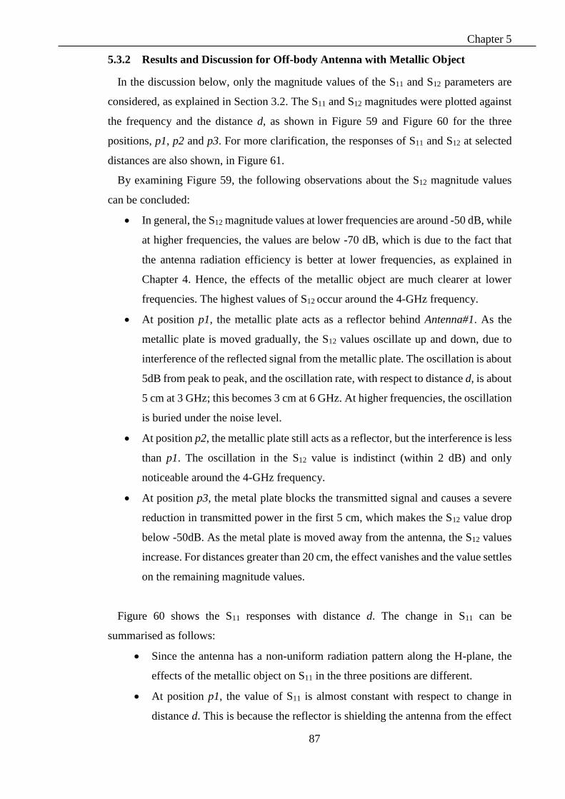
Chapter 5
87
5.3.2 Results and Discussion for Off-body Antenna with Metallic Object
In the discussion below, only the magnitude values of the S11 and S12 parameters are
considered, as explained in Section 3.2. The S11 and S12 magnitudes were plotted against
the frequency and the distance d, as shown in Figure 59 and Figure 60 for the three
positions, p1, p2 and p3. For more clarification, the responses of S11 and S12 at selected
distances are also shown, in Figure 61.
By examining Figure 59, the following observations about the S12 magnitude values
can be concluded:
In general, the S12 magnitude values at lower frequencies are around -50 dB, while
at higher frequencies, the values are below -70 dB, which is due to the fact that
the antenna radiation efficiency is better at lower frequencies, as explained in
Chapter 4. Hence, the effects of the metallic object are much clearer at lower
frequencies. The highest values of S12 occur around the 4-GHz frequency.
At position p1, the metallic plate acts as a reflector behind Antenna#1. As the
metallic plate is moved gradually, the S12 values oscillate up and down, due to
interference of the reflected signal from the metallic plate. The oscillation is about
5dB from peak to peak, and the oscillation rate, with respect to distance d, is about
5 cm at 3 GHz; this becomes 3 cm at 6 GHz. At higher frequencies, the oscillation
is buried under the noise level.
At position p2, the metallic plate still acts as a reflector, but the interference is less
than p1. The oscillation in the S12 value is indistinct (within 2 dB) and only
noticeable around the 4-GHz frequency.
At position p3, the metal plate blocks the transmitted signal and causes a severe
reduction in transmitted power in the first 5 cm, which makes the S12 value drop
below -50dB. As the metal plate is moved away from the antenna, the S12 values
increase. For distances greater than 20 cm, the effect vanishes and the value settles
on the remaining magnitude values.
Figure 60 shows the S11 responses with distance d. The change in S11 can be
summarised as follows:
Since the antenna has a non-uniform radiation pattern along the H-plane, the
effects of the metallic object on S11 in the three positions are different.
At position p1, the value of S11 is almost constant with respect to change in
distance d. This is because the reflector is shielding the antenna from the effect

Chapter 5
88
of the metallic plate.
At position p2, the S11 value changes up and down with a change in distance d,
mainly in the frequencies below 8 GHz; meanwhile, for higher frequencies, the
S11 response is almost constant with the change in distance d. This is related to
the fact that the antenna radiation efficiency below 8 GHz is much higher than
its efficiency above 8 GHz. For distances less than 5cm, the change in the S11
values is around 10dB. For distances greater than 5 cm, the response is settled,
except for the band around the 4-GHz frequency, where the S11 value is still
affected by the change in d.
At position p3, the response of S11 is almost constant, except for slight changes
around the 4-GHz and 6-GHz frequencies. For distances less than 5cm, these
changes are about 5dB and they become less than 2 dB for larger distances.
Figure 59: S12 magnitude for Off-body antenna at position (a) p1, (b) p2 and
(c) p3
(a) (b)
(c)
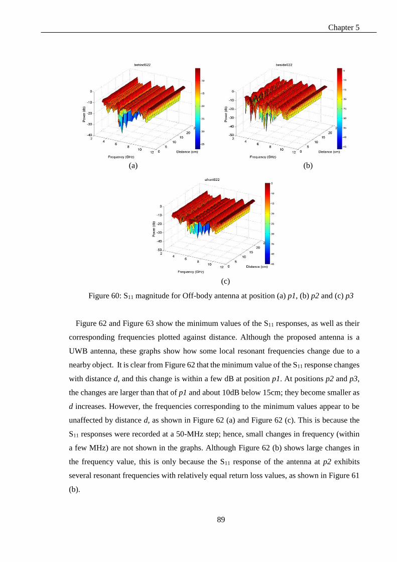
Chapter 5
89
Figure 60: S11 magnitude for Off-body antenna at position (a) p1, (b) p2 and (c) p3
Figure 62 and Figure 63 show the minimum values of the S11 responses, as well as their
corresponding frequencies plotted against distance. Although the proposed antenna is a
UWB antenna, these graphs show how some local resonant frequencies change due to a
nearby object. It is clear from Figure 62 that the minimum value of the S11 response changes
with distance d, and this change is within a few dB at position p1. At positions p2 and p3,
the changes are larger than that of p1 and about 10dB below 15cm; they become smaller as
d increases. However, the frequencies corresponding to the minimum values appear to be
unaffected by distance d, as shown in Figure 62 (a) and Figure 62 (c). This is because the
S11 responses were recorded at a 50-MHz step; hence, small changes in frequency (within
a few MHz) are not shown in the graphs. Although Figure 62 (b) shows large changes in
the frequency value, this is only because the S11 response of the antenna at p2 exhibits
several resonant frequencies with relatively equal return loss values, as shown in Figure 61
(b).
(c)
(a) (b)

Chapter 5
90
Figure 61: Off-body antennas, S12 (left) and S11 (right), at selected distances for three
positions: (a) p1, (b) p2 and (c) p3
(a)
(b)
(c)

Chapter 5
91
Figure 62: Minimum value of the S11 response with distance d, at position (a) p1, (b)
p2 and (c) p3
Figure 63: Frequency corresponding to the minimum value of S11 responses, at
positions (a) p1, (b) p2 and (c) p3
(a) (b)
(c)
(c)
(b) (a)

Chapter 5
92
5.4 On-body Antenna Measurements
This section discusses the changes in an antenna’s S-parameter when it comes into
contact with the human body, as well as a metallic object, through several experiments.
In these experiments, the proposed antenna was mounted on several parts of the human
body and tested inside an anechoic chamber. The antenna diagrams shown in Chapter 4
are redrawn again in Figure 64 and Figure 65 for clarity. Both designs of the antenna,
with a reflector or without a reflector, were used to investigate the benefits of the reflector
in terms of sensitivity to the human body. Then a metallic object was introduced to the
test setup in the near field of the antenna. Section 5.4.1 presents the test setup and results
of the on-body test, while Section 5.4.2 presents the on-body antenna results when a
metallic object is introduced.
Figure 64: Proposed antenna without a reflector: (a) top, (b) bottom and
(c) perspective view
Figure 65: Proposed antenna with a reflector: (a) top, (b) bottom, (c) side and
(d) perspective view
(c)
(c)
(d)

Chapter 5
93
5.4.1 On-body Antenna Measurements without a Passive Object in the Near Field
In this test, two antennas were fixed inside an anechoic chamber, with a 2-m distance
between them. One antenna was fixed on a wooden stand 1 m above the ground, while
the other antenna was mounted on a human body, as shown in Figure 66. The test was
repeated for several human body parts, as shown in Figure 67 and explained below:
Free space: both antennas were fixed on a wooden stand (without the human
body).
On hand #1: antenna #1 was mounted on a human hand (near the wrist)
On hand #2: antenna #1 was mounted on a human hand (near the wrist) and the
volunteer was wearing a wrist watch on the same hand.
On arm: antenna #1 was mounted on a human forearm (the region of the arm
between the elbow and the wrist).
On shoulder #1, #2 and #3: antenna #1 was mounted on a human shoulder at
three different positions, as shown in Figure 67 (b).
In all of these locations, the antennas were placed face-to-face, except for shoulder #2
and shoulder #3, where the antenna was rotated with the human body. The whole test was
repeated for the antenna design with reflector and without reflector.
Figure 66: Top view of on-body test setup inside anechoic chamber
For simplicity, the experimental results were viewed in three groups; each group
compares the antenna performance (with and without a reflector) at a subset of the
locations specified above, as shown in the next three figures. Figure 68 compares the
results of S11 and S12 at the following locations: On-hand#1, On-arm#2 and On-
Shoulder#1. The figure shows that for an antenna with a reflector, the changes in the S11
responses at the three locations are trivial in most of the specified frequency range.
2 m face to face antennas
Human body
Ant #1 Ant #2

Chapter 5
94
Figure 67: Antenna on body location: (a) the positions of the antennas on several
body parts (b) three locations of on-shoulder test
On the other hand, the antenna with a reflector was highly affected by changes to the
antenna’s position on the human body. During the test with the antenna (without the
reflector), it was noticed that the S11 responses change drastically, even with slight
movement on the same location. This is due to the fact that the antenna feed line is placed
directly on the skin; hence, its impedance varies, based on the variation of the contact
area with skin. This also affects S12, as can be seen in Figure 68 (b), where the S12
magnitude values in the low frequencies for the antenna without a reflector are smaller
than those of the antenna with a reflector.
2 m
2 m
2 m
Human body
On-shoulder #1
On-shoulder #2
On-shoulder #3
On hand
On arm
On shoulder #1, #2, #3
(a)
(b)
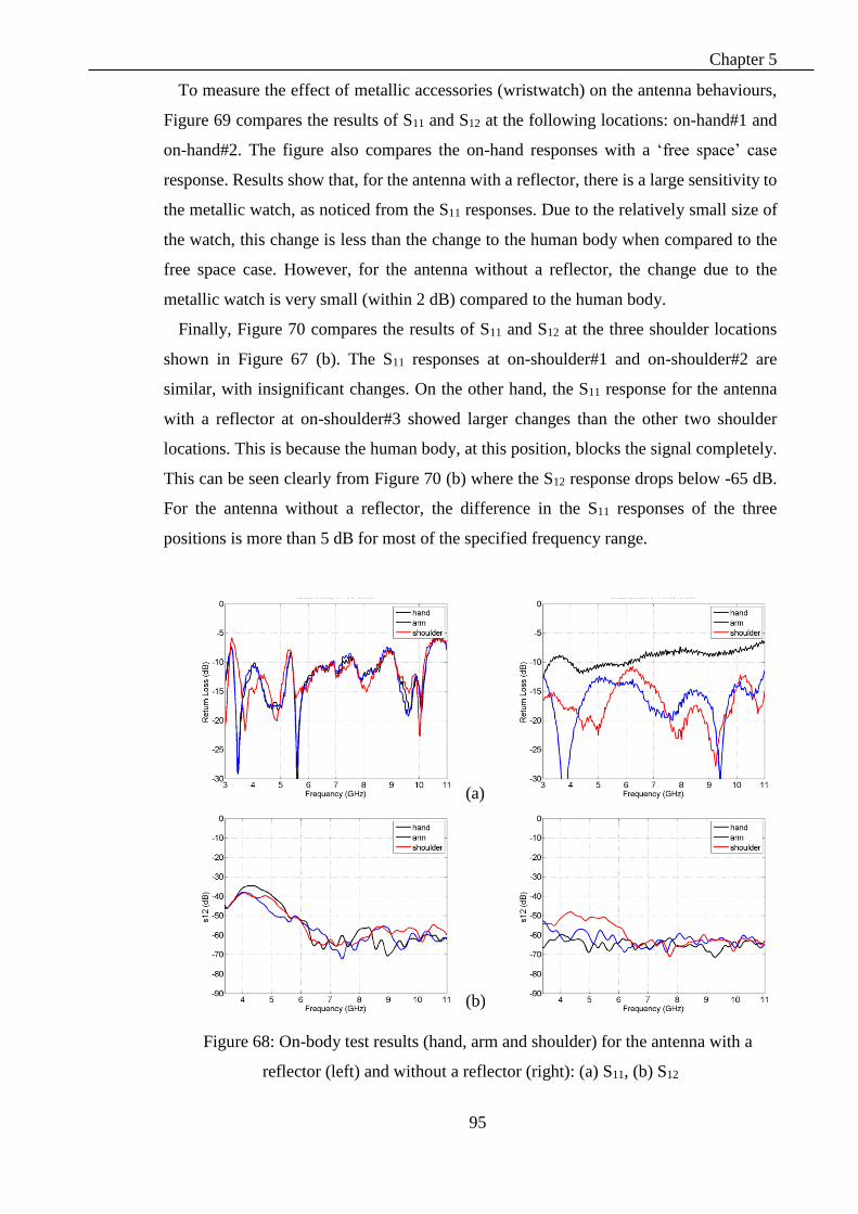
Chapter 5
95
To measure the effect of metallic accessories (wristwatch) on the antenna behaviours,
Figure 69 compares the results of S11 and S12 at the following locations: on-hand#1 and
on-hand#2. The figure also compares the on-hand responses with a ‘free space’ case
response. Results show that, for the antenna with a reflector, there is a large sensitivity to
the metallic watch, as noticed from the S11 responses. Due to the relatively small size of
the watch, this change is less than the change to the human body when compared to the
free space case. However, for the antenna without a reflector, the change due to the
metallic watch is very small (within 2 dB) compared to the human body.
Finally, Figure 70 compares the results of S11 and S12 at the three shoulder locations
shown in Figure 67 (b). The S11 responses at on-shoulder#1 and on-shoulder#2 are
similar, with insignificant changes. On the other hand, the S11 response for the antenna
with a reflector at on-shoulder#3 showed larger changes than the other two shoulder
locations. This is because the human body, at this position, blocks the signal completely.
This can be seen clearly from Figure 70 (b) where the S12 response drops below -65 dB.
For the antenna without a reflector, the difference in the S11 responses of the three
positions is more than 5 dB for most of the specified frequency range.
Figure 68: On-body test results (hand, arm and shoulder) for the antenna with a
reflector (left) and without a reflector (right): (a) S11, (b) S12
(a)
(b)

Chapter 5
96
Figure 69: On-body test results (hand, hand with watch) for the antenna with a
reflector (left) and without a reflector (right): (a) S11 and (b) S12
Figure 70: On-body test results (three shoulder positions) for the antenna with a
reflector (left) and without a reflector (right): (a) S11 and (b) S12
(a)
(b)
(a)
(b)

Chapter 5
97
5.4.2 On-body Antenna Measurements with a Passive Object in the Near Field
This section presents the setup and measurements of an antenna under the effect of both
the human body and a metallic object. The test setup is similar to the one described in the
previous section, with some variations. Antenna#1 was mounted on only one body part
(on arm), and a metallic plate (size 30 cm × 20 cm) was introduced, as shown in Figure
71. The antennas were placed face-to-face, while the metallic plate was placed beside
antenna#1. The distance between antenna#1 and the metallic plate (named d) was varied
from 1 cm to 25 cm, at a step of 1 cm. At each step, the s-parameters of the antenna were
measured and recorded. The whole test was repeated twice, for the antenna design with a
reflector and without a reflector.
Figure 71: Layout (top view) of on-body test with metallic object
Figure 72 shows the responses of S11 and S12 at selected distances for both the antenna
with a reflector and without reflector, while Figure 73 shows the responses for all of the
25 steps. As can be seen in Figure 72, the change in distance d caused a change in the
response of S11. For the antenna with a reflector, the change is within 5 dB and appears
mostly at the resonant frequencies of the S11 response at 3.5 GHz, 5.5 GHz and 8 GHz.
For the antenna without a reflector, the change is higher; it is around 5db in most of the
responses and more than 10 dB in the resonant frequencies regions. The next section
presents the details of the feature extraction methods, to quantify these changes.
Variable distance d
2 m face to face antenna
Human body
Metallic plate
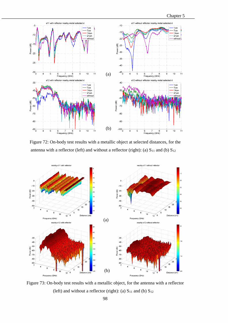
Chapter 5
98
Figure 72: On-body test results with a metallic object at selected distances, for the
antenna with a reflector (left) and without a reflector (right): (a) S11 and (b) S12
Figure 73: On-body test results with a metallic object, for the antenna with a reflector
(left) and without a reflector (right): (a) S11 and (b) S12
(a)
(b)
(a)
(b)

Chapter 5
99
5.5 Proposed indicators for object detection near an on-body antenna
This section proposes two methods that relate the change in the s-parameter response
to distance d, between the antenna and the metallic object within the antenna near field.
Using the data presented in Section 5.4.2, two features are proposed: root-mean-square
and peak-to-peak. The root-mean-square feature at distance d is calculated as follows:
𝑑𝑖𝑓𝑓𝑑 = 𝑆𝑑 − 𝑆𝑓𝑟𝑒𝑒𝑠𝑝𝑎𝑐𝑒
, (44)
𝑟𝑚𝑠𝑑 = 𝑟𝑜𝑜𝑡_𝑚𝑒𝑎𝑛_𝑠𝑞𝑢𝑎𝑟𝑒 (𝑑𝑖𝑓𝑓 𝑑 ) , (45)
where Sd is the S-parameter response (S11 or S12) when the metallic plate is at distance d,
and Sfreespace is the S-parameter response when the metallic plate is not presented.
The peak-to-peak feature at distance d is calculated as follows:
𝑝2𝑝𝑑 = 𝑚𝑎𝑥(𝑑𝑖𝑓𝑓 𝑑 ) − 𝑚𝑖𝑛(𝑑𝑖𝑓𝑓 𝑑 ). (46)
Figure 74 shows the values of the root-mean-square feature of the S11 response, plotted
at each distance step for the antenna design with and without a reflector. In the figure, the
dots represent the calculated rms11 values, while the line represents the fitted data. For the
antenna design with a reflector, the value of the rms11 feature stays relatively constant at
distances less than 10 cm, then the value starts to decrease monotonically with the
distance. On the other hand, the rms feature does not show a direct relation to distance
change for the antenna without reflector. Similarly, the values of the peak-to-peak feature
of the S11 response (shown in Figure 75 ) show a monotonic decrease in the feature value,
with an increase of distances above 10 cm for the design with a reflector, as compared
with the design without a reflector. For the S12 results, equations (1) - (3) were also applied
to the S12 responses at each distance step, to calculate rms12 and p2p12 ; this is shown in
Figure 76. However, the results show the change in the S12 features that is not directly
related to the change in distance d, for the antenna with reflector and without reflector.
In conclusion, the results show that the rms_11 and p2p_11 feature provide indicators for
the object existence near an on-body antenna for distances above 10 cm when the reflector
is used. Further analysis of the data is presented in next section to classify the nearby
object and distinguish between the human body and a metallic object.

Chapter 5
100
Figure 74: rms feature for S11 vs distance d
Figure 75: peak-to-peak feature for S11 vs distance d
Figure 76: S12 features vs distance d: (a) rms and (b) peak-to-peak

Chapter 5
101
5.6 Classification methodology and results for on-body tests
To apply the PCA, data should be arranged in an n × m matrix, where n is the number
of observations and m is the number of variables. The analysis in this section uses the
experimental measurements obtained in Section 5.4. The experimental measurements
were arranged as 32 observations. The first 25 observations represented measurements
for the 25 locations in the experiment, i.e., 25 distance steps. The next 7 measurements
were taken on the human body without a metal plate. Each observation involved the
aggregated frequency responses of the S11 magnitude, S11 phase, S12 magnitude and S12
phase in a single vector, representing the variables. As previously described, each
frequency contains 201 steps from 3GHz to 11GHz; hence, each observation will contain
4 × 201 variables. This classifies the dimension of the data matrix as 32 × 804.
Figure 77 and Figure 78 show the classification of an object or antenna location, based
on the first two principal components, PC1 and PC2, for the antenna with or without a
reflector. Each marker in the figure represents a single observation in which the metallic
object or the antenna is placed at a different location. The marker shape represents a
different measurement.
For the antenna with a reflector, the results in Figure 77 clearly show the ability of the
antenna to detect a nearby object. The blue markers (Ο) in the lower left side of the figure
represent on-body measurements with nearby metallic objects. The black markers (∇) in
the upper left represent the on-body measurements without a metallic object on several
body parts. From the figure, it can be seen that the free space case, where the antenna was
tested without a human body or metallic object, appears within the other cases of on-body
antennas and far from the cases of metallic objects. However, there are two exceptions in
this classification. The first is the case that represents the location of on-hand#2, where
the antenna is placed on hand with a metallic watch. In this case, the corresponding
marker (∇3) appears next to the blue markers, which emphasises the antenna’s ability to
detect metallic objects. The second exception is the case that represents the on-shoulder#3
location, where the antenna is placed on the shoulder and the body was on the line-of-
sight between the two antennas. Due to the large change in the S12 response, the
corresponding marker appears on the far right side of the figure, yet it is separated from
the blue markers.
On the other hand, Figure 78 shows the classification results for the antenna without a
reflector. As can be shown in the figure, the markers corresponding to cases with and
without a metallic object are scattered in the figure and cannot be classified.

Chapter 5
102
Figure 77: PCA classification for the antenna with a reflector
Figure 78: PCA classification for the antenna without a reflector
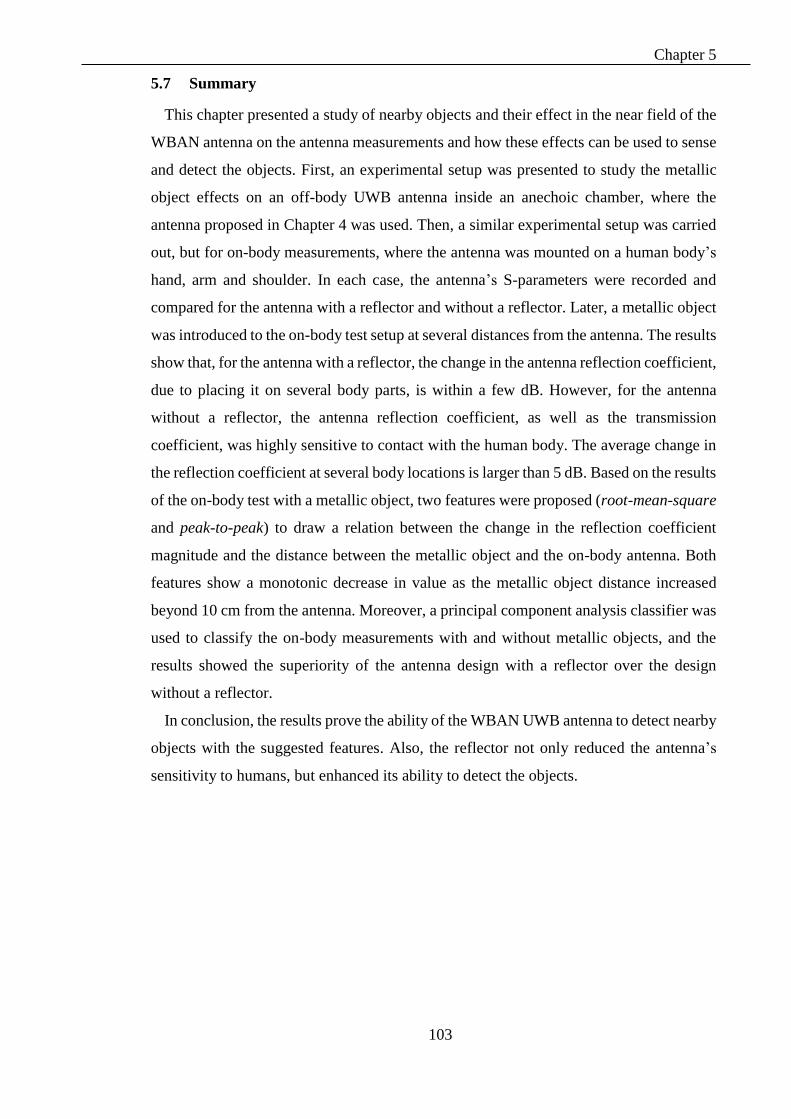
Chapter 5
103
5.7 Summary
This chapter presented a study of nearby objects and their effect in the near field of the
WBAN antenna on the antenna measurements and how these effects can be used to sense
and detect the objects. First, an experimental setup was presented to study the metallic
object effects on an off-body UWB antenna inside an anechoic chamber, where the
antenna proposed in Chapter 4 was used. Then, a similar experimental setup was carried
out, but for on-body measurements, where the antenna was mounted on a human body’s
hand, arm and shoulder. In each case, the antenna’s S-parameters were recorded and
compared for the antenna with a reflector and without a reflector. Later, a metallic object
was introduced to the on-body test setup at several distances from the antenna. The results
show that, for the antenna with a reflector, the change in the antenna reflection coefficient,
due to placing it on several body parts, is within a few dB. However, for the antenna
without a reflector, the antenna reflection coefficient, as well as the transmission
coefficient, was highly sensitive to contact with the human body. The average change in
the reflection coefficient at several body locations is larger than 5 dB. Based on the results
of the on-body test with a metallic object, two features were proposed (root-mean-square
and peak-to-peak) to draw a relation between the change in the reflection coefficient
magnitude and the distance between the metallic object and the on-body antenna. Both
features show a monotonic decrease in value as the metallic object distance increased
beyond 10 cm from the antenna. Moreover, a principal component analysis classifier was
used to classify the on-body measurements with and without metallic objects, and the
results showed the superiority of the antenna design with a reflector over the design
without a reflector.
In conclusion, the results prove the ability of the WBAN UWB antenna to detect nearby
objects with the suggested features. Also, the reflector not only reduced the antenna’s
sensitivity to humans, but enhanced its ability to detect the objects.

104
Chapter 6 CONCLUSIONS AND FUTURE
WORK

Chapter 6
105
6.1 Conclusions
The near-field interaction between wearable devices and the surrounding objects,
especially indoor environments, is an inevitable challenge and drastically affects the
network function. The changes in the antenna impedance due to coupling with a nearby
object is significant within the antenna near field, and these changes can be used as
indicators for passive objects presence. Through an analysis of the changes in the antenna
reflection coefficient, these objects can be detected and their distance to the antenna can
be estimated within the near field. This thesis proposed and described techniques to sense
passive objects nearby WBAN node to improve the interaction between WBAN and its
surrounding environment, through the analysis of node’s antenna measurements and
proposed an antenna design for this purpose.
6.1.1 Near Field Sensing and WBAN State of the Art
The review of recent literature in WBAN showed the importance of nearfield sensing
based on antenna measurements and its role in many applications. The literature review
showed an increase interest in using the antennas as sensors in several applications, e.g.
gesture recognition and localization. Although the channel modelling of a wireless body
area network has been an active topic for researchers in recent years, the effects of near-
field interaction of WBAN with passive objects are not fully addressed. Many
applications use physical-level measurements, such as received signal strength and link
quality indicator, to gain knowledge about changes in the surrounding environment, yet
these measurements become totally distorted in the case of near-field interferer. On the
other hand, adding sensors, such as cameras or a proximity sensor, are a straightforward
solutions to enhance the interaction between WBAN with its surrounding, yet these
solutions complicate the WBAN node design and increases its cost. On the other hand the
review showed lack in the studies of interaction between WBAN and surrounding passive
object. This leaves a gap for research in the area of antenna design and near field
interaction with passive object as well as the inherit interaction with the human body.
6.1.2 Off-Body Near Field Sensing Using Low Profile Antenna
The focus of this stage was to study and analyse the changes in the reflection coefficient
of a low profile antenna due to the existence of a metallic, passive object within the
antenna near field. For this purpose, tests were conducted inside an anechoic chamber

Chapter 6
106
using a low profile, narrow band, dipole antenna. During the tests, a metallic plate was
placed within the antenna near the field at several distances, whereas the antenna itself
was connected to a network analyser, which captured the antenna’s reflection and
transmission coefficients. By analysing the data from the reflection coefficients with a
metallic object at several distances from the antenna, the change in antenna return loss
value and frequency were found to be related to the distance to the metallic object. Then,
a direct relation between the distances to the antenna return loss was concluded.
Furthermore, the object’s location, relative to two communicating low profile antennas,
was detected, using both reflection and transmission coefficients. The magnitude and
phase values of both coefficients for different setups were fed to a PCA classifier. Results
showed the classifier’s ability to classify the object’s location into roughly three groups
relative to the line of sight. Although the experiments were done in free space, without
human interference, they signifies the low profile antenna capabilities in sensing and
detecting nearby objects.
6.1.3 Antenna Design and On-Body Near Field Sensing
Following to the two previous steps, a design for a WBAN antenna was proposed, with
the purpose of achieving low back radiation while maintaining a low profile. The antenna
was based on the widely used Vivaldi antenna, and it was modified to achieve the
radiation pattern that matches WBAN requirements. The modification involves adding a
reflector to both reduce the antenna sensitivity and enhance the radiation pattern.
However, adding a reflector also reduces the antenna’s total efficiency at higher
frequencies. The antenna was optimized in simulation, then it was implemented and tested
inside and anechoic chamber. When the antenna is then tested on several body parts, the
results show very slight changes in the antenna reflection and transmission coefficient
values, compared to the initial test values in free space. More interestingly, the reflector
not only reduced the antenna coupling with the human body, but also enhanced its
sensitivity to the nearby object. This was shown through a set of experiments inside an
anechoic chamber; the proposed antenna was fixed on several body parts, with and
without a reflector, while a metallic object was placed near the antenna. Two indicators
were proposed to detect the object distance to the antenna, based on the root mean square
and the peak to peak difference of the changes in the reflection coefficient. The results
show that the proposed antenna with the reflector is more sensitive to change in nearby
object distances within the near field, compared with the design without a reflector.
Chapter 6
107
Finally, when the classifier was applied, it showed the ability of the design to detect
nearby objects, even when it was fixed on the human body. Both the antenna design and
the proposed features showed the feasibility of using low profile antenna to clearly sense
the passive object presence within the antenna near field and estimate its distance to the
antenna in WBAN.
6.2 Future Work
The results of this research project are promising towards using the low profile
antenna’s measurements to enhance the interaction between a WBAN node and its
surroundings. As stated above, near-field sensing in WBAN is very important, yet it is a
niche research area, except for a few recent attempts. Hence, it is difficult to cover all the
aspects of this system in order to address all of its challenges in one thesis. For future
work, there are several directions for further development and improvement of the current
work, as listed below.
1. In the current study, only two types of antenna were used: a commercial, narrow
band, dipole antenna and the proposed wideband antenna. Analysis of the changes
in antenna measurements is still required for other types of antenna, e.g. textile
antenna [144, 145] and fractal antenna [146, 147]. This is necessary to obtain a
wider view of the relation between near field sensing and the antenna type and
generalizing the concept of near field sensing in WBAN applications.
2. Although the effects of the object shape on the results were discussed in the thesis,
only metallic material (perfect electric conductor) was considered. Moreover, the
tests only focused on detecting the object existence and distance to the antenna but
not detecting its material. Future work based on this thesis should pay attention to
the object material and its effects on the near field sensing process. Objects that are
typically exist in indoor environments and interact with WBAN are expected to be
made of a mix of several materials e.g. metallic and dielectric. By examining
different types of object material, the proposed methods can be applied for not only
wearable body sensor networks, but also robot-based sensors networks [87] for
harsh environments where a lot of metallic and non-metallic objects e.g. pipes and
containers are presented.
3. The signals used in this thesis experiments were applied by the network analyser as
a continuous Gaussian sinusoidal wave for the specified frequency range. Future

Chapter 6
108
work for the near field sensing should consider using a modulated signal that carries
actual data as it normally transmitted in typical WBAN communication. This step
will assure the agility of near field sensing concept as the WBAN node will sense
its surrounding while having an ongoing transmission with other nodes. It also
guarantee the compatibility with the current communication protocols since it
doesn’t require a special transmission mode for sensing. Commercially, several
types of advanced network analysers are available, which can provide S-parameter
measurements, using a modulated signal.
4. During the analysis of the reflection coefficient of the proposed antenna, the
measured changes in frequency domain were less than the changes in the case of
the narrow band antenna. This is due to the resolution of the recorded data, since
the proposed antenna’s response was recorded over a wider frequency band. Finer
measurements of the UWB will give more useful features to sense nearby objects,
e.g. monitoring single resonant frequency within the UWB. This can be achieved
by select and analyse specific parts of the frequency response of the UWB
measurements instead of processing the whole range.
5. In this work, the proposed features and data analysis were based on antenna
measurements obtained only in the frequency domain. Many current WBAN
applications depend on impulse radio transmission for various purposes.
Examination of the effects of passive objects on the WBAN antenna in time domain,
is necessary to extend the near field sensing concept to those types of applications
[148].

109
References
[1] K. M. S. Thotahewa, J.-M. Redouté, and M. R. Yuce, Ultra Wideband Wireless
Body Area Networks: Springer, 2014.
[2] K. Nikita, "Antennas and RF Communication," in Handbook of Biomedical
Telemetry, ed: Wiley-IEEE Press, 2014, pp. 1-736.
[3] G. Yang, Body sensor networks: Second Edition, Springer-Verlag London, 2014.
[4] M. Ilyas and I. Mahgoub, Handbook of sensor networks: compact wireless and
wired sensing systems: CRC press, 2004.
[5] K. Cheng-Hung, W. Sung-Jung, and T. Jenn-Hwan, "A Novel Folded UWB
Antenna for Wireless Body Area Network," IEEE Trans. Antennas and Propag.,
vol. 60, pp. 1139-1142, 2012.
[6] M. Koohestani, J. F. Zurcher, A. A. Moreira, and A. K. Skrivervik, "A Novel,
Low-Profile, Vertically-Polarized UWB Antenna for WBAN," IEEE Trans.
Antennas and Propag., vol. 62, pp. 1888-1894, 2014.
[7] E. E. Lopez Canelon, A. Garcia Loapez, R. Chandra, and A. J. Johansson, "3D
printed miniaturized UWB antenna for wireless body area network," in Antennas
and Propagation (EuCAP), 2014 8th European Conference on, 2014, pp. 3090-
3093.
[8] N. Chahat, M. Zhadobov, R. Sauleau, and K. Ito, "A Compact UWB Antenna for
On-Body Applications," IEEE Trans. Antennas and Propag., vol. 59, pp. 1123-
1131, 2011.
[9] D. L. Paul, H. Giddens, M. G. Paterson, G. S. Hilton, and J. P. McGeehan, "Impact
of Body and Clothing on a Wearable Textile Dual Band Antenna at Digital
Television and Wireless Communications Bands," Antennas and Propagation,
IEEE Transactions on, vol. 61, pp. 2188-2194, 2013.
[10] H. Baldus, S. Corroy, A. Fazzi, K. Klabunde, and T. Schenk, "Human-centric
connectivity enabled by body-coupled communications," Communications
Magazine, IEEE, vol. 47, pp. 172-178, 2009.
[11] G. Koutitas, "Multiple Human Effects in Body Area Networks," Antennas and
Wireless Propagation Letters, IEEE, vol. 9, pp. 938-941, 2010.
[12] M. Koohestani, N. Pires, A. K. Skrivervik, and A. A. Moreira, "Performance
Study of a UWB Antenna in Proximity to a Human Arm," Antennas and Wireless
Propagation Letters, IEEE, vol. 12, pp. 555-558, 2013.
110
[13] A. M. Eid and J. W. Wallace, "Accurate Modeling of Body Area Network
Channels Using Surface-Based Method of Moments," Antennas and Propagation,
IEEE Transactions on, vol. 59, pp. 3022-3030, 2011.
[14] S. H. Kvist, J. Thaysen, and K. B. Jakobsen, "Ear-to-Ear On-Body Channel Model
for Hearing Aid Applications," Antennas and Propagation, IEEE Transactions
on, vol. 63, pp. 344-352, 2015.
[15] W. Qiong, T. Tayamachi, I. Kimura, and W. Jianqing, "An On-Body Channel
Model for UWB Body Area Communications for Various Postures," Antennas
and Propagation, IEEE Transactions on, vol. 57, pp. 991-998, 2009.
[16] H. Sang-Hun and P. Sang Kyu, "Performance analysis of wireless body area
network in indoor off-body communication," Consumer Electronics, IEEE
Transactions on, vol. 57, pp. 335-338, 2011.
[17] A. Chunsu, A. Byoungjik, K. Sunwoo, and C. Jaehoon, "Experimental outage
capacity analysis for off-body wireless body area network channel with transmit
diversity," Consumer Electronics, IEEE Transactions on, vol. 58, pp. 274-277,
2012.
[18] X. Wu, Y. I. Nechayev, C. C. Constantinou, and P. S. Hall, "Interuser Interference
in Adjacent Wireless Body Area Networks," Antennas and Propagation, IEEE
Transactions on, vol. 63, pp. 4496-4504, 2015.
[19] I. Khan, Y. I. Nechayev, K. Ghanem, and P. S. Hall, "BAN-BAN Interference
Rejection With Multiple Antennas at the Receiver," Antennas and Propagation,
IEEE Transactions on, vol. 58, pp. 927-934, 2010.
[20] K. Ghanem, "Effect of Channel Correlation and Path Loss on Average Channel
Capacity of Body-to-Body Systems," Antennas and Propagation, IEEE
Transactions on, vol. 61, pp. 6260-6265, 2013.
[21] B. Jung Nam, C. Young Hoon, K. Jin Young, K. Jang Woo, and K. Dong In,
"Efficient interference cancellation scheme for wireless body area network,"
Communications and Networks, Journal of, vol. 13, pp. 167-174, 2011.
[22] A. L. Martens, P. Slottje, M. Y. Meima, J. Beekhuizen, D. Timmermans, H.
Kromhout, et al., "Residential exposure to RF-EMF from mobile phone base
stations: Model predictions versus personal and home measurements," Science of
The Total Environment, vol. 550, pp. 987-993, 4/15/ 2016.
[23] N. Decarli, F. Guidi, and D. Dardari, "A Novel Joint RFID and Radar Sensor
Network for Passive Localization: Design and Performance Bounds," Selected

111
Topics in Signal Processing, IEEE Journal of, vol. 8, pp. 80-95, 2014.
[24] A. Argyriou, A. Caballero Breva, and M. Aoun, "Optimizing Data Forwarding
from Body Area Networks in the Presence of Body Shadowing with Dual
Wireless Technology Nodes," Mobile Computing, IEEE Transactions on, vol. 14,
pp. 632-645, 2015.
[25] M. Kim and J. I. Takada, "Characterization of Wireless On-Body Channel Under
Specific Action Scenarios at Sub-GHz Bands," Antennas and Propagation, IEEE
Transactions on, vol. 60, pp. 5364-5372, 2012.
[26] S. Swaisaenyakorn, S. W. Kelly, and J. C. Batchelor, "A Study of Factors
Affecting Wrist Channel Characteristics for Walking Postures Using Motion
Capture," Antennas and Propagation, IEEE Transactions on, vol. 62, pp. 2231-
2237, 2014.
[27] A. Hyo-Sung and Y. Wonpil, "Environmental-Adaptive RSSI-Based Indoor
Localization," Automation Science and Engineering, IEEE Transactions on, vol.
6, pp. 626-633, 2009.
[28] T. Sheng-Yuan, C. Kwang-Cheng, and R. Prasad, "Spectrum Sensing of OFDMA
Systems for Cognitive Radio Networks," Vehicular Technology, IEEE
Transactions on, vol. 58, pp. 3410-3425, 2009.
[29] F. Guidi, A. Sibille, and C. Roblin, "Interaction of UWB Tag Backscattering With
Close Metallic Reflectors," Antennas and Wireless Propagation Letters, IEEE,
vol. 13, pp. 245-248, 2014.
[30] L. Xiao zheng, X. Zeming, and C. Xuanliang, "A Compact RFID Reader Antenna
for UHF Near-Field and Far-Field Operations," International Journal of Antennas
and Propagation, vol. 2013, p. 5, 2013.
[31] Q. Xianming and C. Zhi Ning, "Proximity Effects of Metallic Environments on
High Frequency RFID Reader Antenna: Study and Applications," Antennas and
Propagation, IEEE Transactions on, vol. 55, pp. 3105-3111, 2007.
[32] Q. H. Abbasi, M. M. Khan, S. Liaqat, M. Kamran, A. Alomainy, and Y. Hao,
"Experimental investigation of ultra wideband diversity techniques for on-body
radio communications," Progress In Electromagnetics Research C, vol. 34, pp.
165-181, 2013.
[33] Q. H. Abbasi, M. U. Rehman, H. T. Chattha, K. Qaraqe, A. Alomainy, H. Yang,
et al., "Ultra wideband antenna diversity characterisation for off-body
communications in an indoor environment," Microwaves, Antennas &

112
Propagation, IET, vol. 8, pp. 1161-1169, 2014.
[34] K. Li, N. Ahmed, S. S. Kanhere, and S. Jha, "Reliable transmissions in AWSNs
by using O-BESPAR hybrid antenna," Pervasive and Mobile Computing.
[35] W. Wei and Z. Qian, "Toward long-term quality of protection in mobile networks:
a context-aware perspective," Wireless Communications, IEEE, vol. 22, pp. 34-
40, 2015.
[36] L. Bin, Y. Zhisheng, and C. Chang Wen, "MAC protocol in wireless body area
networks for E-health: challenges and a context-aware design," Wireless
Communications, IEEE, vol. 20, pp. 64-72, 2013.
[37] Tobo, x, D. P. n, T. H. Falk, and M. Maier, "Context awareness in WBANs: a
survey on medical and non-medical applications," Wireless Communications,
IEEE, vol. 20, pp. 30-37, 2013.
[38] R. M. Vaghefi, M. R. Gholami, R. M. Buehrer, and E. G. Strom, "Cooperative
Received Signal Strength-Based Sensor Localization With Unknown Transmit
Powers," Signal Processing, IEEE Transactions on, vol. 61, pp. 1389-1403, 2013.
[39] M. R. Gholami, R. M. Vaghefi, and E. G. Strom, "RSS-Based Sensor Localization
in the Presence of Unknown Channel Parameters," Signal Processing, IEEE
Transactions on, vol. 61, pp. 3752-3759, 2013.
[40] C. A. Balanis, Antenna Theory: Analysis and Design: John Wiley & Sons, 2005.
[41] T. S. Rappaport, Wireless Communications: Principles and Practice: Prentice
Hall PTR, 2002.
[42] W. L. Stutzman and G. A. Thiele, Antenna Theory and Design: Wiley, 2012.
[43] T. Prakoso, R. Ngah, Z. Ghassemlooy, and T. A. Rahman, "Antenna
representation in two‐port network scattering parameter," Microwave and Optical
Technology Letters, vol. 53, pp. 1404-1409, 2011.
[44] M. I. Sobhy, B. Sanz-Izquierdo, and J. C. Batchelor, "System and Circuit Models
for Microwave Antennas," Microwave Theory and Techniques, IEEE
Transactions on, vol. 55, pp. 729-735, 2007.
[45] J. T. Aberle, "Two-Port Representation of an Antenna With Application to Non-
Foster Matching Networks," Antennas and Propagation, IEEE Transactions on,
vol. 56, pp. 1218-1222, 2008.
[46] C. C. Y. Poon, B. P. L. Lo, M. R. Yuce, A. Alomainy, and H. Yang, "Body Sensor
Networks: In the Era of Big Data and Beyond," Biomedical Engineering, IEEE
Reviews in, vol. 8, pp. 4-16, 2015.

113
[47] K. Nikita, "Intrabody Communication," in Handbook of Biomedical Telemetry,
ed: Wiley-IEEE Press, 2014, pp. 1-736.
[48] "IEEE Standard for Information technology--Telecommunications and
information exchange between systems Local and metropolitan area networks--
Specific requirements Part 11: Wireless LAN Medium Access Control (MAC)
and Physical Layer (PHY) Specifications," IEEE Std 802.11-2012 (Revision of
IEEE Std 802.11-2007), pp. 1-2793, 2012.
[49] "IEEE Standard for Telecommunications and Information Exchange Between
Systems - LAN/MAN Specific Requirements - Part 11: Wireless Medium Access
Control (MAC) and physical layer (PHY) specifications: High Speed Physical
Layer in the 5 GHz band," IEEE Std 802.11a-1999, pp. 1-102, 1999.
[50] "IEEE Standard for Local and metropolitan area networks--Part 15.4: Low-Rate
Wireless Personal Area Networks (LR-WPANs)," IEEE Std 802.15.4-2011
(Revision of IEEE Std 802.15.4-2006), pp. 1-314, 2011.
[51] ZigBee Alliance. Available: www.zigbee.org (Last accessed: January 2016)
[52] W. Yuan, X. Wang, J.-P. G. Linnartz, and I. M. M. Niemegeers, "Coexistence
Performance of IEEE 802.15.4 Wireless Sensor Networks Under IEEE 802.11b/g
Interference," Wireless Personal Communications, vol. 68, pp. 281-302,
2013/01/01 2013.
[53] G. Wenqi, W. M. Healy, and Z. MengChu, "Impacts of 2.4-GHz ISM Band
Interference on IEEE 802.15.4 Wireless Sensor Network Reliability in
Buildings," Instrumentation and Measurement, IEEE Transactions on, vol. 61,
pp. 2533-2544, 2012.
[54] E. Sarra, H. Moungla, S. Benayoune, and A. Mehaoua, "Coexistence
improvement of wearable body area network (WBAN) in medical environment,"
in Communications (ICC), 2014 IEEE International Conference on, 2014, pp.
5694-5699.
[55] Y. Kim, S. Lee, and S. Lee, "Coexistence of ZigBee-Based WBAN and WiFi for
Health Telemonitoring Systems," Biomedical and Health Informatics, IEEE
Journal of, vol. 20, pp. 222-230, 2016.
[56] "IEEE Standard for Local and metropolitan area networks - Part 15.6: Wireless
Body Area Networks," IEEE Std 802.15.6-2012, pp. 1-271, 2012.
[57] Z. Ya-Li, D. Xiao-Rong, C. C. Y. Poon, B. P. L. Lo, Z. Heye, Z. Xiao-Lin, et al.,
"Unobtrusive Sensing and Wearable Devices for Health Informatics," Biomedical

114
Engineering, IEEE Transactions on, vol. 61, pp. 1538-1554, 2014.
[58] M. Klemm, I. Z. Kovcs, G. F. Pedersen, and G. Troster, "Novel small-size
directional antenna for UWB WBAN/WPAN applications," Antennas and
Propagation, IEEE Transactions on, vol. 53, pp. 3884-3896, 2005.
[59] G. Quintero, J. F. Zurcher, and A. K. Skrivervik, "System Fidelity Factor: A New
Method for Comparing UWB Antennas," Antennas and Propagation, IEEE
Transactions on, vol. 59, pp. 2502-2512, 2011.
[60] K. Do-Hoon, "Effect of antenna gain and group delay variations on pulse-
preserving capabilities of ultrawideband antennas," Antennas and Propagation,
IEEE Transactions on, vol. 54, pp. 2208-2215, 2006.
[61] M. J. Kuhn, Z. Cemin, L. Song, M. R. Mahfouz, and A. E. Fathy, "A system level
design approach to UWB localization," in Microwave Symposium Digest, 2009.
MTT '09. IEEE MTT-S International, 2009, pp. 1409-1412.
[62] G. A. Conway, W. G. Scanlon, C. Orlenius, and C. Walker, "In Situ Measurement
of UHF Wearable Antenna Radiation Efficiency Using a Reverberation
Chamber," Antennas and Wireless Propagation Letters, IEEE, vol. 7, pp. 271-
274, 2008.
[63] T. Alves, B. Poussot, and J. M. Laheurte, "PIFA-Top-Loaded-Monopole Antenna
With Diversity Features for WBAN Applications," Antennas and Wireless
Propagation Letters, IEEE, vol. 10, pp. 693-696, 2011.
[64] P. J. Soh, G. A. E. Vandenbosch, O. Soo Liam, and N. H. M. Rais, "Design of a
Broadband All-Textile Slotted PIFA," Antennas and Propagation, IEEE
Transactions on, vol. 60, pp. 379-384, 2012.
[65] T. Tuovinen, M. Berg, K. Y. Yazdandoost, and J. Iinatti, "Ultra wideband loop
antenna on contact with human body tissues," Microwaves, Antennas &
Propagation, IET, vol. 7, pp. 588-596, 2013.
[66] Z. Shiyu, R. Seager, A. Chauraya, W. Whittow, and Y. Vardaxoglou, "Textile
manufacturing techniques in RF devices," in Antennas and Propagation
Conference (LAPC), 2014 Loughborough, 2014, pp. 182-186.
[67] N. P. I. Kammersgaard, S. H. Kvist, J. Thaysen, and K. B. Jakobsen, "In-the-ear
spiral monopole antenna for hearing instruments," Electronics Letters, vol. 50, pp.
1509-1511, 2014.
[68] R. Chandra and A. J. Johansson, "Antennas and Propagation for In-Mouth
Tongue-Controlled Devices in Wireless Body Area Networks," Antennas and
115
Wireless Propagation Letters, IEEE, vol. 14, pp. 1518-1521, 2015.
[69] D. Gaetano, P. McEvoy, M. J. Ammann, M. John, C. Brannigan, L. Keating, et
al., "Insole Antenna for On-Body Telemetry," Antennas and Propagation, IEEE
Transactions on, vol. 63, pp. 3354-3361, 2015.
[70] A. Hassanien and S. A. Vorobyov, "Transmit Energy Focusing for DOA
Estimation in MIMO Radar With Colocated Antennas," Signal Processing, IEEE
Transactions on, vol. 59, pp. 2669-2682, 2011.
[71] A. Moreira, P. Prats-Iraola, M. Younis, G. Krieger, I. Hajnsek, and K. P.
Papathanassiou, "A tutorial on synthetic aperture radar," Geoscience and Remote
Sensing Magazine, IEEE, vol. 1, pp. 6-43, 2013.
[72] F. Rodriguez-Morales, S. Gogineni, C. J. Leuschen, J. D. Paden, L. Jilu, C. C.
Lewis, et al., "Advanced Multifrequency Radar Instrumentation for Polar
Research," Geoscience and Remote Sensing, IEEE Transactions on, vol. 52, pp.
2824-2842, 2014.
[73] O. Malyuskin and V. F. Fusco, "High-Resolution Microwave Near-Field Surface
Imaging Using Resonance Probes," Instrumentation and Measurement, IEEE
Transactions on, vol. 65, pp. 189-200, 2016.
[74] K. B. Cooper, R. J. Dengler, N. Llombart, B. Thomas, G. Chattopadhyay, and P.
H. Siegel, "THz Imaging Radar for Standoff Personnel Screening," Terahertz
Science and Technology, IEEE Transactions on, vol. 1, pp. 169-182, 2011.
[75] S. Lambot and F. Andre, "Full-Wave Modeling of Near-Field Radar Data for
Planar Layered Media Reconstruction," Geoscience and Remote Sensing, IEEE
Transactions on, vol. 52, pp. 2295-2303, 2014.
[76] J. Wilson and N. Patwari, "Radio Tomographic Imaging with Wireless
Networks," Mobile Computing, IEEE Transactions on, vol. 9, pp. 621-632, 2010.
[77] N. Patwari and J. Wilson, "RF Sensor Networks for Device-Free Localization:
Measurements, Models, and Algorithms," Proceedings of the IEEE, vol. 98, pp.
1961-1973, 2010.
[78] J. Wilson and N. Patwari, "See-Through Walls: Motion Tracking Using Variance-
Based Radio Tomography Networks," Mobile Computing, IEEE Transactions on,
vol. 10, pp. 612-621, 2011.
[79] N. Patwari, J. Wilson, S. Ananthanarayanan, S. K. Kasera, and D. R. Westenskow,
"Monitoring Breathing via Signal Strength in Wireless Networks," Mobile
Computing, IEEE Transactions on, vol. 13, pp. 1774-1786, 2014.

116
[80] K. Woyach, D. Puccinelli, and M. Haenggi, "Sensorless Sensing in Wireless
Networks: Implementation and Measurements," in Modeling and Optimization in
Mobile, Ad Hoc and Wireless Networks, 2006 4th International Symposium on,
2006, pp. 1-8.
[81] M. B. Cover, K. S. Kanukurthy, and D. R. Andersen, "Microwave tomography
using dynamic 802.15.4 wireless networks," in Electro/Information Technology,
2007 IEEE International Conference on, 2007, pp. 251-256.
[82] M. Xufei, T. Shaojie, and L. Xiang-Yang, "Multiple Objects Device-Free Passive
Tracking Using Wireless Sensor Networks," in Communications (ICC), 2011
IEEE International Conference on, 2011, pp. 1-5.
[83] M. Seifeldin, A. Saeed, A. E. Kosba, A. El-Keyi, and M. Youssef, "Nuzzer: A
Large-Scale Device-Free Passive Localization System for Wireless
Environments," Mobile Computing, IEEE Transactions on, vol. 12, pp. 1321-
1334, 2013.
[84] R. C. Qiu, M. C. Wicks, L. Li, Z. Hu, S. J. Hou, P. Chen, et al., "Wireless
tomography, Part I: A novel approach to remote sensing," in Waveform Diversity
and Design Conference (WDD), 2010 International, 2010, pp. 000244-000256.
[85] R. C. Qiu, Z. Hu, M. C. Wicks, S. J. Hou, L. Li, and J. L. Gary, "Wireless
tomography, Part II: A system engineering approach," in Waveform Diversity and
Design Conference (WDD), 2010 International, 2010, pp. 277-282.
[86] Z. Peng and R. C. Qiu, "Wireless tomography, Part III: Compressed sensing for
ultra-wideband signals," in Waveform Diversity and Design Conference (WDD),
2010 International, 2010, pp. 35-39.
[87] V. Rampa, F. Vicentini, S. Savazzi, N. Pedrocchi, M. Ioppolo, and M. Giussani,
"Safe human-robot cooperation through sensor-less radio localization," in
Industrial Informatics (INDIN), 2014 12th IEEE International Conference on,
2014, pp. 683-689.
[88] P. Qifan, G. Sidhant, G. Shyamnath, and P. Shwetak, "Whole-home gesture
recognition using wireless signals," presented at the Proceedings of the 19th
annual international conference on Mobile computing and networking, Miami,
Florida, USA, 2013.
[89] Microsoft Inc. Kinect for Xbox One. Available: http://www.xbox.com/en-
GB/xbox-one/accessories/kinect-for-xbox-one#fbid=ZOcL-NlxldP (Last
accessed January 2016)

117
[90] Whole-Home Gesture Recognition Using Wireless, Computer Science &
Engineering, University of Washington. Available:
http://wisee.cs.washington.edu (Last accessed: January 2016)
[91] G. Cohn, D. Morris, S. Petal, and D. Tan. Humantenna: Sensing Gestures Using
the Body as an Antenna. Available: http://research.microsoft.com/en-
us/um/redmond/groups/cue/humantenna/ (Last accessed: January 2016)
[92] Y.-J. An, B.-J. Jang, and J.-G. Yook, "Detection of human vital signs and
estimation of direction of arrival using multiple doppler radars," Journal of
Electromagnetic Engineering And Science, vol. 10, pp. 250-255, 2010.
[93] D. Obeid, S. Sadek, G. Zaharia, and G. E. Zein, "Doppler radar for heartbeat rate
and heart rate variability extraction," in E-Health and Bioengineering Conference
(EHB), 2011, 2011, pp. 1-4.
[94] Y. J. An, G. H. Yun, and J. G. Yook, "Sensitivity Enhanced Vital Sign Detection
Based on Antenna Reflection Coefficient Variation," Biomedical Circuits and
Systems, IEEE Transactions on, vol. PP, pp. 1-1, 2015.
[95] A. A. Serra, P. Nepa, G. Manara, G. Corsini, and J. L. Volakis, "A Single On-
Body Antenna as a Sensor for Cardiopulmonary Monitoring," Antennas and
Wireless Propagation Letters, IEEE, vol. 9, pp. 930-933, 2010.
[96] R. Bhattacharyya, C. Floerkemeier, and S. Sarma, "Low-Cost, Ubiquitous RFID-
Tag-Antenna-Based Sensing," Proceedings of the IEEE, vol. 98, pp. 1593-1600,
2010.
[97] C. Tsirmpas, A. Rompas, O. Fokou, and D. Koutsouris, "An indoor navigation
system for visually impaired and elderly people based on Radio Frequency
Identification (RFID)," Information Sciences, vol. 320, pp. 288-305, 11/1/ 2015.
[98] A. R. J. Ruiz, F. S. Granja, J. C. Prieto Honorato, and J. I. G. Rosas, "Accurate
Pedestrian Indoor Navigation by Tightly Coupling Foot-Mounted IMU and RFID
Measurements," Instrumentation and Measurement, IEEE Transactions on, vol.
61, pp. 178-189, 2012.
[99] I. Mohammad and H. Huang, "Monitoring fatigue crack growth and opening using
antenna sensors," Smart Materials and Structures, vol. 19, p. 055023, 2010.
[100] C. Occhiuzzi, C. Paggi, and G. Marrocco, "Passive RFID Strain-Sensor Based on
Meander-Line Antennas," Antennas and Propagation, IEEE Transactions on, vol.
59, pp. 4836-4840, 2011.
[101] M. J. Cazeca, J. Mead, J. Chen, and R. Nagarajan, "Passive wireless displacement

118
sensor based on RFID technology," Sensors and Actuators A: Physical, vol. 190,
pp. 197-202, 2/1/ 2013.
[102] Project Soli, Google Inc. Available: www.google.com/atap/project-soli (Last
accessed: January 2016)
[103] A. Yong-Jun, Y. Gi-Ho, K. Sung Woo, and Y. Jong-Gwan, "Wrist Pulse Detection
System Based on Changes in the Near-Field Reflection Coefficient of a
Resonator," Microwave and Wireless Components Letters, IEEE, vol. 24, pp. 719-
721, 2014.
[104] B. Pottier and L. Rasolofondraibe, "Capacitive Sensor Dedicated to Pedestrians
Protection," Sensors Journal, IEEE, vol. 15, pp. 5886-5892, 2015.
[105] CST Microwave Studio, CST Computer Simulation Technology AG. Available:
www.cst.com/Products/CSTMWS (Last accessed: January 2016)
[106] J. Shlens. A Tutorial on Principal Component Analysis: Derivation, Discussion
and Singular Value Decomposition (2003). Available:
https://www.cs.princeton.edu/picasso/mats/PCA-Tutorial-Intuition_jp.pdf (Last
accessed: January 2016)
[107] I. T. Jolliffe, Principal Component Analysis: Springer, 2002.
[108] M. Linting, "Nonparametric inference in nonlinear principal components analysis:
exploration and beyond," Data Theory Group, Department of Education, Faculty
of Social and Behavioural Sciences, Leiden University, 2007.
[109] A. Buja and N. Eyuboglu, "Remarks on Parallel Analysis," Multivariate
Behavioral Research, vol. 27, p. 509, 1992.
[110] J. J. Martinez, M. A. Campbell, M. S. Warden, E. B. Hughes, N. J. Copner, and
A. J. Lewis, "Dual-Sweep Frequency Scanning Interferometry Using Four Wave
Mixing," Photonics Technology Letters, IEEE, vol. 27, pp. 733-736, 2015.
[111] A. Anghel, G. Vasile, R. Cacoveanu, C. Ioana, and S. Ciochina, "Short-Range
Wideband FMCW Radar for Millimetric Displacement Measurements,"
Geoscience and Remote Sensing, IEEE Transactions on, vol. 52, pp. 5633-5642,
2014.
[112] M. Elhoushi, J. Georgy, A. Noureldin, and M. J. Korenberg, "Motion Mode
Recognition for Indoor Pedestrian Navigation Using Portable Devices,"
Instrumentation and Measurement, IEEE Transactions on, vol. 65, pp. 208-221,
2016.
[113] Y. Jun, "Toward physical activity diary: motion recognition using simple

119
acceleration features with mobile phones," presented at the Proceedings of the 1st
international workshop on Interactive multimedia for consumer electronics,
Beijing, China, 2009.
[114] R. Cavallari, F. Martelli, R. Rosini, C. Buratti, and R. Verdone, "A Survey on
Wireless Body Area Networks: Technologies and Design Challenges," IEEE
Comm. Surveys & Tutorials, , vol. 16, pp. 1635-1657, 2014.
[115] Y.-f. Wei and C. Roblin, "Multislot Antenna with a Screening Backplane for
UWB WBAN Applications," International Journal of Antennas and Propagation,
vol. 2012, p. 12, 2012.
[116] T. Castel, P. Van Torre, E. Tanghe, S. Agneessens, G. Vermeeren, xfc, et al.,
"Improved Reception of In-Body Signals by Means of a Wearable Multi-Antenna
System," International Journal of Antennas and Propagation, vol. 2013, p. 9,
2013.
[117] W. Amer, G. Y. Tian, and C. Tsimenidis, "Sensing passive object existence within
an antenna near field based on return loss," in Antennas and Propagation
Conference (LAPC), 2014 Loughborough, 2014, pp. 400-404.
[118] S. Wen-Tron, J. Shiou-Chiau, and T. Jenn-Hwan, "A Reduced-Size Wide Slot
Antenna for Enhancing Along-Body Radio Propagation in UWB On-Body
Communications," IEEE Trans. Antennas and Propag., vol. 62, pp. 1194-1203,
2014.
[119] P. J. Gibson, "The Vivaldi Aerial," in Microwave Conference, 1979. 9th
European, 1979, pp. 101-105.
[120] W. Sung-Jung and M. Tzyh-Ghuang, "A Wideband Slotted Bow-Tie Antenna
With Reconfigurable CPW-to-Slotline Transition for Pattern Diversity," Antennas
and Propagation, IEEE Transactions on, vol. 56, pp. 327-334, 2008.
[121] W. Ya-Wei, W. Guang-Ming, and Z. Bin-Feng, "Directivity Improvement of
Vivaldi Antenna Using Double-Slot Structure," Antennas and Wireless
Propagation Letters, IEEE, vol. 12, pp. 1380-1383, 2013.
[122] K. Ebnabbasi, D. Busuioc, R. Birken, and W. Ming, "Taper Design of Vivaldi and
Co-Planar Tapered Slot Antenna (TSA) by Chebyshev Transformer," Antennas
and Propagation, IEEE Transactions on, vol. 60, pp. 2252-2259, 2012.
[123] B. Jian, S. Shouyuan, and D. W. Prather, "Modified Compact Antipodal Vivaldi
Antenna for 4-50-GHz UWB Application," IEEE Trans. Microwave Theory and
Techniques, vol. 59, pp. 1051-1057, 2011.
120
[124] F. Peng, J. Yong-Chang, H. Wei, and Z. Fu-Shun, "A Miniaturized Antipodal
Vivaldi Antenna With Improved Radiation Characteristics," IEEE Trans.
Antennas and Propag., vol. 10, pp. 127-130, 2011.
[125] W. Jiangniu, Z. Zhiqin, N. Zaiping, and L. Qing-Huo, "A Printed UWB Vivaldi
Antenna Using Stepped Connection Structure Between Slotline and Tapered
Patches," IEEE Antennas Wireless Propag. Lett., vol. 13, pp. 698-701, 2014.
[126] W. Qiong, R. Hahnel, Z. Hui, and D. Plettemeier, "On-body directional antenna
design for in-body UWB wireless communication," in Antennas and Propagation
(EUCAP), 2012 6th European Conference on, 2012, pp. 1011-1015.
[127] W. Amer, T. Gui Yun, and C. Tsimenidis, "A novel, low-profile, directional UWB
antenna for WBAN," in Antennas and Propagation Conference (LAPC), 2014
Loughborough, 2014, pp. 708-710.
[128] H. G. Schantz, The Art and Science of Ultra-Wideband Antennas, 1St Edition ed.:
Artech House Print on Demand, 2005.
[129] A. G. Yarovoy, R. Pugliese, J. H. Zijderveld, and L. P. Ligthart, "Antenna
development for UWB impulse radio," in Microwave Conference, 2004. 34th
European, 2004, pp. 1257-1260.
[130] W. S. T. Rowe and R. B. Waterhouse, "Reduction of backward radiation for CPW
fed aperture stacked patch antennas on small ground planes," Antennas and
Propagation, IEEE Transactions on, vol. 51, pp. 1411-1413, 2003.
[131] S. D. Targonski, D. M. Pozar, and R. B. Waterhouse, "Aperture-coupled
microstrip antennas using reflector elements for wireless communications," in
Antennas and Propagation for Wireless Communications, 1998. 1998 IEEE-APS
Conference on, 1998, pp. 163-166.
[132] W. Wiesbeck, G. Adamiuk, and C. Sturm, "Basic Properties and Design Principles
of UWB Antennas," Proceedings of the IEEE, vol. 97, pp. 372-385, 2009.
[133] C. M. Kruesi, R. J. Vyas, and M. M. Tentzeris, "Design and Development of a
Novel 3-D Cubic Antenna for Wireless Sensor Networks (WSNs) and RFID
Applications," IEEE Trans. Antennas and Propag., vol. 57, pp. 3293-3299, 2009.
[134] M. M. Khan, Q. H. Abbasi, A. Alomainy, H. Yang, and C. Parini, "Experimental
characterisation of ultra-wideband off-body radio channels considering antenna
effects," Microwaves, Antennas & Propagation, IET, vol. 7, pp. 370-380, 2013.
[135] D. B. Smith, D. Miniutti, T. A. Lamahewa, and L. W. Hanlen, "Propagation
Models for Body-Area Networks: A Survey and New Outlook," Antennas and

121
Propagation Magazine, IEEE, vol. 55, pp. 97-117, 2013.
[136] S. L. Cotton, "A Statistical Model for Shadowed Body-Centric Communications
Channels: Theory and Validation," Antennas and Propagation, IEEE
Transactions on, vol. 62, pp. 1416-1424, 2014.
[137] R. Di Bari, Q. H. Abbasi, A. Alomainy, and Y. Hao, "An advanced UWB channel
model for body-centric wireless networks," progress in electromagnetics
research, vol. 136, pp. 79-99, 2013.
[138] R. G. Garcia-Serna, C. Garcia-Pardo, and J. M. Molina-Garcia-Pardo, "Effect of
the Receiver Attachment Position on Ultrawideband Off-Body Channels,"
Antennas and Wireless Propagation Letters, IEEE, vol. 14, pp. 1101-1104, 2015.
[139] N. Yamamoto, N. Shirakata, D. Kobayashi, K. Honda, and K. Ogawa, "BAN
Radio Link Characterization Using an Arm-Swinging Dynamic Phantom
Replicating Human Walking Motion," Antennas and Propagation, IEEE
Transactions on, vol. 61, pp. 4315-4326, 2013.
[140] Q. H. Abbasi, A. Sani, A. Alomainy, and H. Yang, "Experimental
Characterization and Statistical Analysis of the Pseudo-Dynamic Ultrawideband
On-Body Radio Channel," Antennas and Wireless Propagation Letters, IEEE,
vol. 10, pp. 748-751, 2011.
[141] S. Manzari, C. Occhiuzzi, and G. Marrocco, "Feasibility of Body-Centric Systems
Using Passive Textile RFID Tags," Antennas and Propagation Magazine, IEEE,
vol. 54, pp. 49-62, 2012.
[142] P. A. Catherwood and W. G. Scanlon, "Body-centric ultra-wideband multi-
channel characterisation and spatial diversity in the indoor environment,"
Microwaves, Antennas & Propagation, IET, vol. 7, pp. 61-70, 2013.
[143] M. Bosiljevac, Z. Sipus, and A. K. Skrivervik, "Propagation in Finite Lossy
Media: An Application to WBAN," Antennas and Wireless Propagation Letters,
IEEE, vol. 14, pp. 1546-1549, 2015.
[144] R. Moro, S. Agneessens, H. Rogier, A. Dierck, and M. Bozzi, "Textile Microwave
Components in Substrate Integrated Waveguide Technology," Microwave Theory
and Techniques, IEEE Transactions on, vol. 63, pp. 422-432, 2015.
[145] Z. Wang, J. L. Volakis, and A. Kiourti, "10 - Embroidered antennas for
communication systems A2 - Dias, Tilak," in Electronic Textiles, ed Oxford:
Woodhead Publishing, 2015, pp. 201-237.
[146] A. Farswan, A. K. Gautam, B. K. Kanaujia, and K. Rambabu, "Design of Koch

122
Fractal Circularly Polarized Antenna for Handheld UHF RFID Reader
Applications," Antennas and Propagation, IEEE Transactions on, vol. 64, pp.
771-775, 2016.
[147] H. Orazi and H. Soleimani, "Miniaturisation of the triangular patch antenna by the
novel dual-reverse-arrow fractal," Microwaves, Antennas & Propagation, IET,
vol. 9, pp. 627-633, 2015.
[148] A. T. Mobashsher and A. M. Abbosh, "Near-field time-domain characterisation
of wideband antennas," Electronics Letters, vol. 51, pp. 2076-2078, 2015.

123
APPENDIX A: PRINCIPAL COMPONENT
ANALYSIS
This appendix present background of PCA method and how to calculate its statistical
significance. Section A.1 shows the step by step calculations of the PCA results presented
earlier in this thesis, while Section A.2 lists MATLAB code used for PCA calculation.
Finally, Section A.3 lists MATLAB code for the permutation test used in the statistical
significance study.
A.1 Data Preparation and Classification Algorithm
PCA is a multivariate statistical analysis method which transforms the magnitude and phase
responses of the S-parameters into uncorrelated eigenvectors or principal components (PCs)
corresponding to the maxi-mum variability within the data. The PCs are weighted sums of
the original variables. The first PC accounts for the largest variation in the data. Subsequent
PCs correspond to the remaining variability. PCA was used in this work to extract the most
dominant trends in data and link these trends to the effects of nearby object at several
locations around the antenna. The principal components was calculated using the following
procedure [106, 107]:
1. Prepare the data:
The input data should be arranged in m×n matrix, where m is the number of
observations and n is the number of variables. For example, in the first approach discussed
in Section 3.4, the variables for each observation was formed as follow:
𝐴𝑖 = |𝑆11| ,
𝐵𝑖 = ∠ 𝑆11 ,
𝐶𝑖 = |𝑆12| , and
𝐷𝑖 = ∠ 𝑆12 …(A.1)
where each one of these vectors contain 1×201elements, and
𝑋𝑖 = [ 𝐴𝑖 𝐵𝑖 𝐶𝑖 𝐷𝑖] … (A.2)

124
is 1×804 vector that represent the variables of the ith observation .
Each observation correspond to results from one test. The test was repeated for three
different location of the metallic object around the antenna, with 25 distance steps at each
location, hence there are 75 observations. Four more tests were conducted without the
presence of the metallic object. Therefore, the final data set X consist of 79×804 elements
and calculated as follow:
𝑋 = [
𝑋1
𝑋2
⋮𝑋79
] … (A.3)
2. Subtract off the mean variable-wise (row-wise):
3. Calculate the covariance matrix:
𝐶𝑜𝑣𝑋 = (
𝑣𝑎𝑟(𝑋1) 𝑐𝑜𝑣(𝑋1, 𝑋2) ⋯ 𝑐𝑜𝑣(𝑋1, 𝑋79)𝑐𝑜𝑣(𝑋2, 𝑋1) 𝑐𝑜𝑣(𝑋2, 𝑋2) ⋯ 𝑐𝑜𝑣(𝑋2, 𝑋79)
⋮ ⋮ ⋱ ⋮𝑐𝑜𝑣(𝑋79, 𝑋1) 𝑐𝑜𝑣(𝑋79, 𝑋2) ⋯ 𝑣𝑎𝑟(𝑋79)
) … (A.4)
4. Find the eigenvectors EX and eigenvalues from the symmetric matrix 𝑋𝑇𝑋
5. Sort the eigenvectors matrix in decreasing order according to the Eigenvalues
diagonal matrix.
6. Generate PCA component space (PCA scores) by multiplying eigenvectors matrix
with the mean subtracted X:
𝑃𝐶𝐴 = 𝐸𝑋 𝑋 … (A.5)
7. Since the PCA matrix is sorted in descending order, only the first component PC1 and
PC2 were considered in the results discussion.
8. In the second approach of Section 3.4, the input data set was formed as follow:
𝑋 = [
𝑋1
𝑋2
⋮𝑋79
] … (A.6)

125
where each observation Xi is 1×5 vector set that represent five features extracted from the
ith observation as follow:
𝑋𝑖 = [ 𝐹1𝑖 𝐹2𝑖 𝐹3𝑖 𝐹4𝑖 𝐹5𝑖] … (A.7)
And the covariance matrix is calculated as follow:
𝐶𝑜𝑣𝑋 = (
𝑣𝑎𝑟(𝑋1) 𝑐𝑜𝑣(𝑋1, 𝑋2) ⋯ 𝑐𝑜𝑣(𝑋1, 𝑋5)𝑐𝑜𝑣(𝑋2, 𝑋1) 𝑐𝑜𝑣(𝑋2, 𝑋2) ⋯ 𝑐𝑜𝑣(𝑋2, 𝑋5)
⋮ ⋮ ⋱ ⋮𝑐𝑜𝑣(𝑋5, 𝑋1) 𝑐𝑜𝑣(𝑋5, 𝑋2) ⋯ 𝑣𝑎𝑟(𝑋5)
) … (A.8)
A.2 MATLAB Code for PCA Calculation
%Prepare the data
data=[s11mag s11phase s12mag s12phase]; [M,N] = size(data);
% subtract off the mean for each dimension mn = mean(data,2); data = data - repmat(mn,1,N);
% calculate the covariance matrix covariance = 1 / (N-1) * data * data';
% find the eigenvectors and eigenvalues [PC, V] = eig(covariance);
% extract diagonal of matrix as vector V = diag(V);
% sort the variances in decreasing order [junk, rindices] = sort(-1*V); V = V(rindices); PC = PC(:,rindices);
% project the original data set signals = PC' * data;
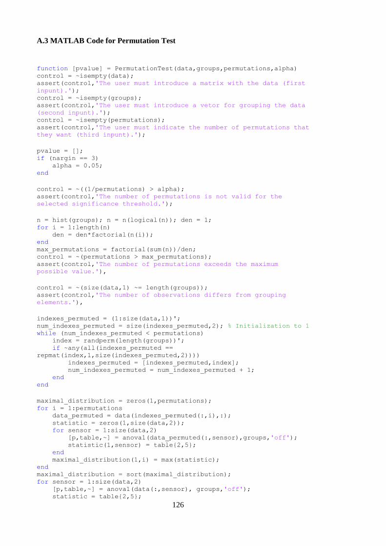
126
A.3 MATLAB Code for Permutation Test
function [pvalue] = PermutationTest(data,groups,permutations,alpha) control = ~isempty(data); assert(control,'The user must introduce a matrix with the data (first
inpunt).'); control = ~isempty(groups); assert(control,'The user must introduce a vetor for grouping the data
(second inpunt).'); control = ~isempty(permutations); assert(control,'The user must indicate the number of permutations that
they want (third inpunt).');
pvalue = []; if (nargin == 3) alpha = 0.05; end
control = ~((1/permutations) > alpha); assert(control,'The number of permutations is not valid for the
selected significance threshold.');
n = hist(groups); n = n(logical(n)); den = 1; for i = 1:length(n) den = den*factorial(n(i)); end max_permutations = factorial(sum(n))/den; control = ~(permutations > max_permutations); assert(control,'The number of permutations exceeds the maximum
possible value.'),
control = ~(size(data,1) ~= length(groups)); assert(control,'The number of observations differs from grouping
elements.'),
indexes_permuted = (1:size(data,1))'; num_indexes_permuted = size(indexes_permuted,2); % Initialization to 1 while (num_indexes_permuted < permutations) index = randperm(length(groups))'; if ~any(all(indexes_permuted ==
repmat(index,1,size(indexes_permuted,2)))) indexes_permuted = [indexes_permuted,index]; num_indexes_permuted = num_indexes_permuted + 1; end end
maximal_distribution = zeros(1,permutations); for i = 1:permutations data_permuted = data(indexes_permuted(:,i),:); statistic = zeros(1,size(data,2)); for sensor = 1:size(data,2) [p,table,~] = anova1(data_permuted(:,sensor),groups,'off'); statistic(1,sensor) = table{2,5}; end maximal_distribution(1,i) = max(statistic); end maximal_distribution = sort(maximal_distribution); for sensor = 1:size(data,2) [p,table,~] = anova1(data(:,sensor), groups,'off'); statistic = table{2,5};

127
c = min(find(maximal_distribution > statistic)); pvalue(sensor) = (permutations-c)/permutations; end
end