cross–sectoral variation in the volatility of plant–level idiosyncratic...
TRANSCRIPT

Cross–Sectoral Variation in The Volatility of
Plant–Level Idiosyncratic Shocks∗
Rui Castro† Gian Luca Clementi‡ Yoonsoo Lee§
This version: June 14, 2013
[Link to the latest version]
Abstract
We estimate the volatility of plant–level idiosyncratic shocks in the U.S. man-ufacturing sector. Our measure of volatility is the variation in Revenue TotalFactor Productivity which is not explained by either industry– or economy–widefactors, or by establishments’ characteristics. Consistent with previous studies,we find that idiosyncratic shocks are much larger than aggregate random distur-bances, accounting for about 80% of the overall uncertainty faced by plants. Theextent of cross–sectoral variation in the volatility of shocks is remarkable. Plantsin the most volatile sector are subject to about six times as much idiosyncraticuncertainty as plants in the least volatile. We provide evidence suggesting thatidiosyncratic risk is higher in industries where the extent of creative destructionis likely to be greater.
Key words: Schumpeterian Competition, Creative Destruction, Product Turnover,R&D Intensity, Investment–Specific Technological Change.
JEL Codes: D24, L16, L60, O30, O31.
∗We thank Alan Sorensen and two anonymous referees for suggestions that greatly improvedthe paper. We are also grateful to Mark Bils, Yongsung Chang, Sılvia Goncalves, MassimilianoGuerini, Francisco Ruge–Murcia, and Carlos Serrano for very helpful comments. A special thankgoes to Gianluca Violante and Jason Cummins for providing us with their data on investment–specific technological change, and to Yongsung Chang and Jay Hong for supplying us with theirELI–SIC correspondence table. The views expressed in this article are those of the authors and donot necessarily reflect the position of the Federal Reserve Bank of Cleveland or the Federal ReserveSystem. The research in this paper was conducted while Yoonsoo Lee was a Special Sworn Statusresearcher of the U.S. Census Bureau at the Michigan Census Research Data Center. Research resultsand conclusions expressed are those of the authors and do not necessarily reflect the views of theCensus Bureau. This paper has been screened to ensure that no confidential data is revealed. Supportfor this research at the Michigan RDC from NSF (awards no. SES–0004322 and ITR–0427889) isgratefully acknowledged. Castro and Lee acknowledge financial support from SSHRC and SogangResearch Frontier Grant, respectively. An earlier draft of this paper circulated under the title “Cross-Sectoral Variation in Firm-Level Idiosyncratic Risk.”
†Department of Economics and CIREQ, Universite de Montreal. Email:[email protected]. Web: https://www.webdepot.umontreal.ca/Usagers/castroru/MonDepotPublic
‡Department of Economics, Stern School of Business, New York University, NBER, and RCEA.Email: [email protected]. Web: people.stern.nyu.edu/gclement/
§Department of Economics, Sogang University and Federal Reserve Bank of Cleveland. Email:[email protected]. Web: http://www.clevelandfed.org/Research/Economists/lee/index.cfm

1 Introduction
In this study we assess the cross–sectoral variation in the volatility of plant–level
idiosyncratic shocks in U.S. manufacturing. Our data consists of a large panel ex-
tracted from the Annual Survey of Manufacturers (ASM), gathered by the US Census
Bureau.
Our measure of volatility is the variation in Revenue Total Factor Productivity
(TFPR) which cannot be forecasted by means of factors, either known or unknown
to the econometrician, that are systematically related to plant dynamics. Variation
in TFPR reflects changes in technical efficiency, as well as shifts in input supply
and product demand schedules affecting input and product prices, respectively. We
strive to isolate the portion of such variation which is due to plant–specific, random
disturbances – a measure of idiosyncratic uncertainty, or risk.
Consistent with previous studies, we find that across the manufacturing sector id-
iosyncratic uncertainty accounts for the majority – about 80% – of overall plant–level
uncertainty. The variation in idiosyncratic risk across 3–digit industries is substan-
tial. To gain a flavor of the amount of heterogeneity we uncover, consider that the
volatility of TFPR growth due to idiosyncratic shocks ranges from 6.7% for producers
of leather soles to a whopping 35.2% for manufacturers of non–ferrous metals.
Why does volatility differ so much across sectors? We provide some preliminary
evidence in favor of a particular explanation: volatility is higher in sectors where cre-
ative destruction is more important. The notion of creative destruction is central to
the Schumpeterian paradigm. According to the latter, firms are engaged in a perpet-
ual race to innovate. Creation, i.e. the success by a laggard in implementing a new
process or producing a new good, displaces the previous market leader, eliminating
(destroying) its rent.
Formal models of Schumpeterian competition1 predict a positive cross–sectoral
association between creative destruction, product turnover, and innovation–related
activities. We document that idiosyncratic risk is higher in industries where product
turnover is greater and investment–specific technological progress is faster.
Our study of the statistical properties of TFPR is of central relevance to most
modern models of business dynamics, where TFPR is the most important, if not
the only driver of establishment growth and survival. See for example the seminal
work of Ericson and Pakes (1995) and Hopenhayn (1992), as well as the more recent
1We refer to the economic growth literature that builds on Aghion and Howitt (1992).
1

information–based theories of Quadrini (2003) and Clementi and Hopenhayn (2006).
Establishment growth is driven by improvement in technical efficiency, increases in
mark–ups, and declines in input prices. Changes of the opposite sign lead plants to
shrink and, eventually, exit.
Learning about the volatility of the innovation to productivity is important in
light of the rather general result that, everything else equal, higher volatility implies
greater reallocation of inputs across plants and greater plant turnover. Over the last
25 years or so, a large number of cross–sectional studies have documented a wide
heterogeneity in the level of total factor productivity across plants. See Bartelsman
and Doms (2000) and Syverson (2011) for a very effective account of this literature.
A related body of work, closer to ours in spirit, studies the extent of cross–plant
variation in the growth of productivity. Davis and Haltiwanger (1992) and Davis,
Haltiwanger, and Schuh (1996) document the extent of within–sector job reallocation
across manufacturing plants, while Davis, Haltiwanger, Jarmin, and Miranda (2006)
describe the time variation in the volatility of business growth rates. Work by Bar-
telsman and Dhrymes (1998), Baily, Hulten, and Campbell (1992), Baily, Bartelsman,
and Haltiwanger (2001) and Foster, Haltiwanger, and Krizan (2001) shows that such
heterogeneity is accompanied by a substantial variation in productivity growth.
Our contribution to the literature is twofold. To start with, we strive to asses the
portion of volatility in plant–level TFPR growth that is due to merely idiosyncratic
shocks.
The logarithm of TFPR is modeled as a linear function of its lagged value, size,
age, a sector–time dummy variable that accounts for aggregate and industry–wide
disturbances, and an establishment–level dummy that stands in for plant unobserved
characteristics systematically associated with productivity dynamics. We regard the
residuals of this regressions as realizations of random shocks, and their standard
deviation as our measure of idiosyncratic risk.
Furthermore, we illustrate the cross–sectoral variation in plant–level idiosyncratic
shocks. We provide estimates of risk by 3–digit SIC sectors and make a first attempt
at identifying the determinants of the heterogeneity we uncover. As a by–product, our
exercise also produces estimates for the sector–specific auto–correlation coefficients of
TFPR.
Given that firms’ stakeholders have often limited insurance opportunities, assess-
ing establishment–level idiosyncratic risk is relevant for the analysis of scenarios where
risk aversion matters. This is the case of entrepreneurship studies such as Michelacci
2

and Schivardi (2013), where idiosyncratic uncertainty hinders business creation via its
negative effect on the value of starting new ventures. In information–based theories
of economic development such as Castro, Clementi, and MacDonald (2004, 2009),
greater idiosyncratic risk is associated with lower capital accumulation via its neg-
ative effect on entrepreneurs’ ability to secure external finance for their investment
projects. Finally, idiosyncratic uncertainty is often cited among the factors restraining
innovative activity. See for example Caggese (2012).
The evidence of lack of risk diversification abounds. Herranz, Krasa, and Villamil
(2009) find that 2% of the primary owners of the firms sampled by the 1998 Survey of
Small Business Finance2 invested more than 80% of their personal net worth in their
firms; 8% invested more than 60%, and about 20% invested more than 40%. Clementi
and Cooley (2009) document that in 2006, more than 20% of CEOs of U.S. publicly–
traded concerns3 held more than 1% of their companies’ common stock. About 10%
held more than 5%. Given the large capitalization of such companies, this information
points to limited portfolio diversification for these individuals.
Understanding how idiosyncratic risk varies across industries is important because
the cross–sectoral heterogeneity in risk, when interacted with other features of the
economic environment, often generates restrictions on the data that are key to refute
economic models. Castro, Clementi, and MacDonald (2009) propose a multi–sector
model where incomplete risk–sharing induces cross–sectoral differences in the return
on investment in favor of lower–risk sectors. According to their theory, the differences
are larger, the poorer is risk–sharing. It turns out that, as long as sectors producing
investment goods are riskier than those producing consumption goods, their model
has a chance at rationalizing well–established evidence on the cross–country variation
of investment rate and the relative price of capital goods. This is a clear case in which
model falsification relies on the knowledge of the cross–sectoral variation in volatility.
In Cunat and Melitz (2010), labor market regulations result in greater inefficien-
cies in sectors with greater idiosyncratic uncertainty. A testable implications is that
countries featuring lower institutional rigidity should specialize in higher–volatility
sectors. Once again, knowledge of the cross–sectoral variation of idiosyncratic risk is
needed in order to falsify their theory.
2The SSBF, administered by the Board of Governors of the Federal Reserve System, surveys alarge cross–sectional sample of non–farm, non–financial, non–real estate firms with less than 500employees.
3The data is from EXECUCOMP, a proprietary database maintained by Standard & Poor’s thatcontains information about compensation of up to 9 executives of all companies quoted in organizedexchanges in the U.S.
3
Three other papers, by Abraham and White (2006), Gourio (2008), and Bachman
and Bayer (2013), share our goal of estimating processes for plant– or firm–level id-
iosyncratic shocks. Their data is from the U.S. Census’ LRD, Deutsche Bundesbank’s
USTAN, and Compustat, respectively. Beyond the data source, our work differs from
theirs on the emphasis we place on the cross–sectoral heterogeneity.4
We are not the first to document the extent of cross–sectoral variation in volatility.
However, data considerations limit the analysis of previous studies to the variation
of sales growth across large firms. See Chun, Kim, Mork, and Yeung (2008), Castro,
Clementi, and MacDonald (2009), and Cunat and Melitz (2010).5 Our data has
other advantages. Given the sample size, it allows us to work with a very fine sector
classification. Furthermore, the sampling technique ensures that it is representative
of the population of manufacturing plants.
The remainder of the paper is organized as follows. The data and methodology
are described in Section 2. Our volatility estimates across 3–digit industries are illus-
trated in Sections 3. In Section 4 we provide evidence in support of the conjecture
that idiosyncratic risk is greater in industries where creative destruction is more im-
portant. In Section 5 we show that, consistent with what found by Castro, Clementi,
and MacDonald (2009) for public firms, plants that produce capital goods are sys-
tematically riskier than their counterparts producing consumption goods. Finally,
Section 6 concludes.
2 Data and Methodology
2.1 Data
We use the Annual Survey of Manufactures (ASM) and the Census of Manufacturers
for the years 1972 through 1997. Our unit of observation is the establishment, defined
as the minimal unit where production takes place, and our analysis is carried out at
the 3–digit SIC sectoral level, which maps into 4– and 5–digit NAICS. Depending on
the year, our data comprises from 50,000 to 70,000 establishments, distributed among
4Campbell, Lettau, Malkiel, and Xu (2001) are also concerned with assessing idiosyncratic risk.Their proxy for the latter, however, is quite different. They decomposed the volatility of excess stockreturns in three components: aggregate, industry–wide, and firm–level. This allowed them to obtainaverage measures of idiosyncratic risk for the whole economy and for several coarsely defined sectors.Their methodology delivers reasonable proxies for the risk borne by equity investors, but not for thatfaced by other stakeholders, such as the owners of small firms.
5In the cross–country study by Michelacci and Schivardi (2013), the proxy for risk is built followingthe methodology of Campbell, Lettau, Malkiel, and Xu (2001).
4

140 3–digit SIC manufacturing industries.
The ASM allows us (i) to compute reliable estimates of plants’ capital stocks,
which are needed to compute TFP indicators and, being a panel rather than a cross–
section, (ii) to use fixed effects to control for unobserved plant characteristics.
The main drawback is that our data is limited to manufacturing. The Census
Bureau’s Longitudinal Business Database (LBD) has a broader coverage. However,
since it does not contain information on capital stocks, it is not suited to computing
plant–level TFP.
2.2 Methodology
Our measure of productivity is known in the literature as real revenue per unit input,
or Revenue Total Factor Productivity (TFPR). Following Foster, Haltiwanger, and
Krizan (2001), Baily, Hulten, and Campbell (1992), and Syverson (2004a) among
others, the (log) TFPR for plant i in 3–digit sector j at time t is
ln zijt ≡ ln yijt − αkιt ln kijt − αℓ
ιt ln ℓijt − αmιt lnmijt, (1)
where yijt is real sales, kijt is capital, ℓijt is labor, and mijt is materials. Real sales
are the nominal value of shipments, deflated using the 4—digit industry–specific de-
flator from the NBER manufacturing productivity database. The details about the
estimation of the residuals in (1) are relegated to Appendix A.2.
The input elasticities are allowed to vary both over time and within 3–digit in-
dustries – the index ι denotes the plant’s 4–digit SIC code. This is important for our
results in Section 4, as it severely limits the concern that sectors characterized by
greater creative destruction display higher volatility in the residuals simply because
they are also characterized by greater unmodeled time and cross–plant variation in
the elasticities.
As effectively pointed out by Foster, Haltiwanger, and Syverson (2008), changes
in the TFPR indicator reflect fluctuations in productive efficiency, as well as shifts in
product demand and input supply schedules leading to updates in input and output
prices. This definition is well suited for our study, as we are interested in identifying
all sources of idiosyncratic uncertainty. Our objective is to estimate the volatility of
those innovations to TFPR that i) are plant–specific and ii) are not systematically
related to observable or unobservable plant characteristics.
We model TFPR as
ln zijt = ρj ln zij,t−1 + µi + δjt + βj ln(size)ijt +
3∑
s=1
ψjsDijts + εijt. (2)
5

The dummy variable µi is a plant–specific fixed effect that accounts for unobserved
persistent heterogeneity across plants. The variable δjt denotes a full set of sector–
specific year dummies, which control for sector–wide shocks and cross–sectoral differ-
ences in business cycle volatility. Size is measured by the number of employees. With
Dijts we denote three categories of age dummies: Young, Middle–Aged, and Mature.
We include size and age because both were shown to be negatively correlated with
plant growth.6
The objects of interest are the estimated residuals εijt, which we will interpret as
realizations of plant–specific shocks. An obvious caveat is that the residuals may also
reflect measurement error and predictable changes in TFPR not accounted for in (2).
This must be kept in mind when considering the magnitude of the volatility estimates
reported below.
Recall that our main goal is to charactere the extent to which the standard devi-
ation of such shocks varies across sectors. We satisfy our curiosity by fitting a simple
log–linear model to the variance of the residuals. We posit that
ln ε2ijt = θj + vijt, (3)
where θj is a sector–specific dummy variable. Letting θj denote its point estimate, our
measure of the conditional standard deviation of TFPR growth for plants in sector j
is√
γ exp(θj), where γ is our estimate of the mean of the random variable exp(vijt).7
In what follows, we will refer to it as volatility of TFPR growth or as idiosyncratic
risk.
3 Volatility Estimates
Our measure of idiosyncratic uncertainty across all manufacturing plants – obtained
by estimating (3) without sector dummies – is 20.53%. This figure is very close to
what implied by the findings of Foster, Haltiwanger, and Syverson (2008), and only
slightly higher than the value reported by Abraham and White (2006), 16.5%. Most
likely, this difference is accounted for by Abraham and White (2006)’s decision to
restrict attention to plants with more than 15 observations, decision that biases their
sample towards older and possibly less volatile establishments.
6See Hall (1987) and Evans (1987).7If vijt were normally distributed, a consistent estimator of E [exp(vijt)] would be exp(σ2/2),
where σ2 is the variance of the residuals in (3). Since the normality assumption is easily rejected,we estimated γ by regressing the squared residuals on the exp of the fitted values generated by (3),without a constant.
6

We gauge the importance of idiosyncratic risk versus aggregate risk by computing a
more comprehensive measure of plant–level uncertainty, which also reflects the portion
that may be ascribed to industry–wide and economy–wide factors. Such measure is
obtained by means of the methodology introduced in the previous section, amended
to exclude the sector–year dummies δjt from the specification of (2).
Our point estimate for overall volatility is 26.16%. It follows that idiosyncratic
factors appear to account for about 80% of overall plant–level uncertainty. Consistent
with studies employing alternative methodologies, such as Campbell, Lettau, Malkiel,
and Xu (2001) and Bachman and Bayer (2013), we find that idiosyncratic risk is
substantially larger than aggregate risk.
0
.05
.1
.15
.2
.25
Fra
ctio
n
0 .1 .2 .3 .4 .5 .6Volatility in sales
0
.05
.1
.15
.2
.25
Fra
ctio
n
0 .1 .2 .3 .4 .5 .6Volatility in TFPR
Figure 1: Histogram of idiosyncratic risk by sector.
Our volatility estimates across 3–digit industries are reported in Table 5 and
illustrated in the right panel of Figure 1, where sectors are sorted by the magnitude
of TFPR volatility. The height of each bin is the fraction of sectors whose estimated
risk falls in the associated interval.
The range of estimates is rather wide. The volatility is lowest for Boot and Shoe
Cut Stock (SIC 313), at 6.7%, and highest in Primary Smelting and Refining of
7

Nonferrous Metals (357), at 35.2%.
As a by–product, our exercise also produces estimates for the sector–specific auto–
correlation coefficients of TFPR. Our values, reported in Table 5 and illustrated in the
right panel of Figure 2, can serve as guidance for the quantitative studies of industry
dynamics that model plant–level TFPR as a serially correlated stochastic process.
See for example Clementi and Palazzo (2013), Lee and Mukoyama (2009), and Khan
and Thomas (2008). The simple arithmetic means of the coefficients is 0.439, a value
very close to what reported by Abraham and White (2006).8
0
.1
.2
.3
Fra
ctio
n
0 .1 .2 .3 .4 .5 .6 .7 .8 .9AR coefficient (sales)
0
.1
.2
.3
Fra
ctio
n
0 .1 .2 .3 .4 .5 .6 .7 .8 .9AR coefficient (TFPR)
Figure 2: Histogram of autocorrelation coefficients by sector.
3.1 Sales
For the purpose of comparison with the rather large literature focusing on sales
growth,9 we repeated our analysis substituting sales for TFPR in equation (2). The
mean standard deviation of the residuals across all manufacturing plants is 29.51%,
8When we weigh sectors by the value of shipments, the mean autocorrelation drops slightly, to0.431.
9See for example Davis, Haltiwanger, Jarmin, and Miranda (2006).
8

larger than above. This is likely to be the case because the scale of production reacts
to shocks, no matter their nature, amplifying their impact on sales.
The range of sectoral estimates is also wider than for TFPR. See Table 5. The
lowest volatility is also attained in the Boot and Shoe Cut Stock sector (313), with
11.3%, while the highest pertains to Railroad Equipment (374), with 53.7%. The
orderings delivered by the TFPR and sales measures are fairly consistent, but not
quite the same. The Spearman’s rank–correlation coefficient is 0.66.
3.2 Censoring
Since we do not explicitly account for exit selection, one may wonder whether the
cross–sectoral variation in volatility that we uncover were simply the result of cen-
soring. Say that the standard deviation of shocks were the same across industries,
but plants in different sectors were burdened by different fixed costs of operation. In
most models of industry dynamics, the selection induced by such heterogeneity would
generate cross–sectoral difference in measured volatility.
To assess the likelihood that the cross–sectoral variation we uncover is indeed
the result of differences in cost structure, consider the model introduced by Hopen-
hayn (1992). In that framework, under very general conditions, sectors characterized
by higher fixed costs will feature higher exit thresholds (in TFPR space) and lower
measured volatility, but also higher exit rates.
Using data from the Statistics of US Businesses Database gathered by the US Cen-
sus Bureau, we computed exit rates across 3–digit SIC industries and plotted them
against our volatility estimates.10 See Figure 3. On average, more volatile industries
tend to display higher exit rates. This finding suggests that the cross–sectoral hetero-
geneity that we uncover cannot be simply the result of censoring. However, we cannot
rule out that censoring indeed biases our estimates, possibly affecting the ranking of
sectors by volatility.11
4 Creative Destruction and Volatility
Why does volatility differ so much across sectors? In this section, we look for evidence
in favor of a particular explanation: volatility is higher in sectors where the speed
and extent of creative destruction are greater.
10Exit rates refer to 1997, the only year in which SUSB and our dataset overlap.11In his study of the ready–mixed concrete industry, Syverson (2004a) finds that markets with
denser construction activity have higher lower-bound productivity levels. This heterogeneity has anobvious impact on the measures of productivity dispersion across markets.
9

201 202
203
204205
206
207
208209
212 213
214
221222
223224
225226
227228
229
231232
233
234
235236 238
239
241
242
243
244 245
249251
252
253
254
259
261
262263
265
267271
272273
274
275
276
277
278
279
281
282
283
284
285
286
287
289
291
295
299301302305306
308
311
313
314
315
316
317
319
321
322323
324
325
326
327
328
329
331332
333
334335336
339
341 342343
344
345346
347
348
349351352
353354
355 356
357
358
359
361362363
364
365 366367
369
371
372
373374
375
376
379
381382384
385
386
387391
393
394
395
396
399
0.1
.2.3
.4T
FP
R V
olat
ility
−20 −15 −10 −5 0Percent change in establishments due to deaths
Figure 3: Volatility and Exit Rates.
Joseph Schumpeter envisioned economic progress as the result of a perpetual race
between innovators. Success by a laggard or an outsider in implementing a new
process or producing a new good, provides them with a competitive advantage and
displaces the previous market leader, eliminating its rent. This, in a nutshell, is the
process of creative destruction.12
We conjecture that most of the plant–level volatility that we document reflects
the turnover between market participants which is at the center of Schumpeter’s
paradigm. That is, we argue that a large fraction of the fluctuations in a plant’s
TFPR is due to variations in its distance from the technology frontier.
Our strategy consists in looking for sector–specific attributes that are likely to
be systematically associated with the speed of turnover. Starting with Aghion and
Howitt (1992), Schumpeter’s idea was formalized in a large number of models. We
turn to this literature for guidance.
In Aghion and Howitt (1992), the producer endowed with the leading technol-
12According to this definition of creative destruction, the elimination of its rent will lead theprevious leader to exit from a specific product market, but not necessarily to cease operations.
10

ogy monopolizes the intermediate good market. Technology improves as a result of
purposeful research and development, which in equilibrium is only carried out by
prospective entrants. When it succeeds in obtaining a new and more productive vari-
ety of intermediate good, the innovator enters and displaces the monopolist. It follows
that all the variation in TFPR is associated with product turnover.
The positive association between product turnover and plant–level volatility is
not specific to Aghion and Howitt (1992). Rather, it is a robust feature of all of
its generalizations in which intermediate goods of different vintages are vertically
differentiated. For example, see Aghion, Harris, Howitt, and Vickers (2001) and
Aghion, Bloom, Bludell, Griffith, and Howitt (2005).
The race can also be among plants that are not directly engaged in R&D, but adopt
components which embed innovations made by others. This is the scenario described
by Copeland and Shapiro (2013), who model the personal computers industry. The
adoption decision, which entails the introduction of a new product, leads to a rise in
sales for the adopter, and to a decline for its competitors.
In Samaniego (2009), the decision that yields a competitive advantage is that of
acquiring the latest vintage of equipment. The faster is investment–specific techno-
logical change, the more frequent is technology adoption by either laggards or new
entrants. In turn, this leads to a more frequent turnover in industry leadership and
more variability in both sales and TFPR.13
In the next section, we ask whether product turnover is indeed higher in industries
where plants are documented to face a greater volatility of TFPR. In Sections 4.2 and
4.3 we will ask whether across sectors our volatility measure is positively related
with the intensity of R&D and the speed of investment–specific technological change,
respectively.
It should be clear that our methodology cannot establish causality. Our – more
limited – goal is to establish whether simple unconditional correlations are consistent
with our conjecture on the origin of the cross–sectoral variation in volatility that we
uncover.
4.1 Product Turnover
The U.S. Bureau of Labor Statistics collects prices on 70,000–80,000 non–housing
goods and services from around 22,000 outlets across various locations. When a
13Obviously R&D and investment-specific technical change may be – most likely are – verticallyrelated. This is the case because an innovation generated by R&D may turn profitable only whenembodied in new capital. See Lach and Rob (1996).
11

product is discontinued, the agency starts collecting prices of a closely related good
at the same outlet, and records the substitution information. The BLS classifies goods
in narrowly–defined categories known as entry–level items (ELI).
Our proxy for turnover is the average monthly frequency of substitutions, known
as the item substitution rate. It is the fraction of goods in the ELI that are replaced on
average every month. Our data is drawn from Bils and Klenow (2004)’s tabulations,
which in turn are based on information on more than 300 consumer good categories
from 1995 to 1997.14
Using the algorithm developed by Chang and Hong (2006), we were able to match
each one of 59 3–digit SIC manufacturing sectors with at least one ELI. For 21 sectors,
the correspondence is one–to–one. The remaining 38 are matched to several among
213 items. In such cases, we defined the substitution rate as the average of the
associated ELIs’ rates, weighted by their respective CPI weights.
Two caveats are worth mentioning. To start with, the BLS data focuses on con-
sumer goods. Most investment good sectors are missing. Furthermore, the substi-
tution rate only tells about the frequency of product turnover and does not provide
information about the size of the step, i.e. the extent to which a new product improves
over the pre–existing one.
The scatter plot in Figure 4 shows that our proxy for product turnover is positively
associated with TFPR volatility. The sample correlation coefficient is 0.43.
Three sectors stand out, as they are characterized by high volatility and re-
markably high substitution rates. They are Computer and Office Equipment (357),
Women’s and Misses’ Outerwear (233), and Girls’ and Children’s Outerwear (236).
Anecdotal evidence as well as scholarly research15 suggest that SIC 357 epitomizes
the idea of creative destruction. However, product turnover in the other two sectors
is not likely to be driven by technological improvements.
Idiosyncratic risk and turnover are positively associated even when we exclude
SIC 233, 236, and 357. However, the correlation coefficient drops to 0.08.16
The last two columns in Table 1 report the results of regressing TFPR volatility
on the average substitution rate and a constant. Column 3 tells us that on average,
14The BLS distinguishes between two types of substitutions. Substitutions are comparable whenthe replacement does not represent a quality improvement over the previous item. They are non-comparable, otherwise. Since average and noncomparable average item substitution rates are highlycorrelated across good categories, our results did not change much when we used non–comparableitem substitution rates instead.
15See Copeland and Shapiro (2013) and citations therein.16For sales volatility, the correlation coefficient is 0.45. Without SIC 233, 236, and 357, it drops to
0.32.
12

201
202
203
204
205
206
207
208
209
225
227
231232
233
234
236238
239
243
251
259
267
271272
273
283
284
285
289
291
295
299301
308
314
316322
326
342
343
352
357
358
363
364
365
366 371
373
384
385
386
387
391
393
394
395
399
.15
.2
.25
.3
.35
.4
.45S
ales
Vol
atili
ty
0 5 10 15 20Average item substitution rate
Raw correlation: 0.45; (excluding 233,236,357): 0.32.
201202
203
204205
206
207
208
209
225
227
231232
233
234
236238
239243
251
259
267271
272273
283
284
285
289
291
295
299301308
314
316
322
326
342343
352
357
358
363
364
365366
371
373384
385
386
387
391
393
394
395
399
.15
.2
.25
.3
.35
.4
.45
TF
PR
Vol
atili
ty
0 5 10 15 20Average item substitution rate
Raw correlation: 0.43; (excluding 233,236,357): 0.08.
Figure 4: Idiosyncratic Risk and Product Substitution Rate.
a 1 percentage point higher substitution rate implies a 0.48 percentage point higher
TFPR volatility. Without SIC 233, 236, and 357 (see column 4), the coefficient
becomes insignificant.17
Some establishments in the ASM are likely to produce more than one product.
Possibly, many more. As long as the correlation between sales from different lines of
business is less than 1, plant–level sales volatility will be lower than average volatility
at the level of product line. This may explain why sectors such as Glass and Glassware
(322), Books (273), and Household Furniture (251) are characterized by a relatively
high item substitution rate and low volatility of TFPR.
4.2 R&D Intensity
Unfortunately we lack data on research and development expenditure in the ASM.
We measure a sector’s research intensity as the ratio of R&D expenditure to sales
in COMPUSTAT. The latest CENSUS–NSF R&D survey found that most of the
17Our standard errors of this and the following sections have been computed by a bootstrap pro-cedure aimed at addressing the generated regressor problem.
13

Table 1: Idiosyncratic Risk and Product Substitution Rate.
Dependent Variable: Sales Volatility TFPR Volatility
(1) (2) (3) (4)
Substitution Rate 0.0076∗∗∗ 0.0085∗∗ 0.0048∗∗∗ 0.0013(0.0022) (0.0037) (0.0018) (0.0025)
Constant 0.2581∗∗∗ 0.2549∗∗∗ 0.1889∗∗∗ 0.2008∗∗∗
(0.0123) (0.0157) (0.0091) (0.0106)
Observations 58 55 58 55R2 0.2060 0.1003 0.1877 0.0062
Bootstrap standard errors in parenthesis.∗∗∗Significant at 1%. ∗∗Significant at 5%. ∗Significant at 10%.
Specifications in columns (2) and (4) exclude SIC 233, 236, and 357.
research and development activity takes place at large firms. This leads us to think
that the cross–sectoral variation in R&D expenditures in the population is not likely
to differ much from that for large, public firms.
The cross–industry variation in research expenditures that we uncover is substan-
tial. Our measure of research intensity varies from 0.022% for Book Binding (SIC
278) to 7.77% for firms in Drugs (283).
The unconditional relationship between our risk proxy and research intensity is
illustrated in Figure 5. In Table 2 we report the results of regressing volatility on
R&D intensity and a constant. In the case of TFPR, the coefficient of R&D intensity
Table 2: Idiosyncratic Risk and Research Intensity.
Dependent Variable: Sales Volatility TFPR Volatility
R&D Intensity 0.4359 0.7509∗∗∗
(0.3467) (0.2246)
Constant 0.2832∗∗∗ 0.1918∗∗∗
(0.0084) (0.0055)
Observations 115 115R2 0.0129 0.0865
Bootstrap standard errors in parenthesis.∗∗∗Significant at 1%. ∗∗Significant at 5%. ∗Significant at 10%.
is statistically and economically significant. A 1 percentage point increase in research
intensity implies an increase in volatility of about 0.75 percentage points.
14

201
202
203
204
205
206
207
208
209
221222
225
227
232
233
234239
242
243
245
251252253
254 259
261
262263265
267
271272
273 274275
276
278
279
281
282283
284
285
286
287
289291
295
299301
302
305306
308
314321
322323
324325
326327
329331
332
333334
335
336339341
342
343
344
345
346347
348
349
351
352
353
354 355
356
357
358
359
361362
363
364
365366
367
369371
372
373
374
375
376
379
381
382384
385
386
387
391393
394
395
396
399
.05
.15
.25
.35
.45
.55S
ales
Vol
atili
ty
0 .02 .04 .06 .08R&D Intensity
Raw correlation: 0.11.
201202
203
204205206
207
208209
221222
225
227
232
233
234
239
242
243
245251
252
253
254
259
261
262263
265
267271
272273
274
275
276
278
279
281
282
283
284
285
286
287
289
291
295
299301302 305306
308314
321
322323
324
325
326
327
329
331332
333
334 335336
339
341 342343
344
345346
347
348
349351352
353354
355356
357
358
359
361362363
364
365 366367
369
371
372
373374
375
376
379
381 382384
385
386
387391
393
394
395
396
399
.05
.15
.25
.35
.45
.55
TF
PR
Vol
atili
ty
0 .02 .04 .06 .08R&D Intensity
Raw correlation: 0.29.
Figure 5: Idiosyncratic Risk and R&D.
Since Grilliches (1979), the relation between R&D and productivity has been
the object of interest for a large number of studies. The results described above
are consistent with recent findings by Doraszelski and Jaumandreu (2013). For a
large sample of Spanish manufacturing firms, they establish that engaging in R&D
introduces uncertainties in the productivity process that would be absent otherwise.
4.3 Investment–Specific Technological Change
In a simple two–sector model where investment and consumption goods are produced
competitively, the quality improvement in the investment good equals the negative
of the change in its relative price. Exploiting this restriction, Cummins and Violante
(2002) computed time series of quality improvement – or technological change – for
a variety or equipment goods over the period 1948–2000.
Using detailed data on capital expenditures by 2–digit SIC industries provided
by the Bureau of Economic Analysis, Cummins and Violante (2002) also constructed
measures of investment–specific technological change by sector. In this section we ask
whether such measures are systematically related to our proxies for risk.
15

20
21
22
23
24
25
26
27
28
29
30
31
32
3334
35
36
38
39
.1
.15
.2
.25
.3
.35
.4S
ales
Vol
atili
ty
.025 .03 .035 .04 .045 .05Investment−specific technical change
Raw correlation (excluding 27): 0.39.
2021
22
23
24
25
26
27
28
29
30
31323334
3536
38
39
.1
.15
.2
.25
.3
.35
.4
TF
PR
Vol
atili
ty
.025 .03 .035 .04 .045 .05Investment−specific technical change
Raw correlation (excluding 27): 0.47.
Figure 6: Idiosyncratic Risk and Investment–Specific Technological Change.
Given the level of aggregation in the data on technological change, our analysis
is confined to 18 2–digit SIC sectors, listed in Table 6. For each industry, the rate of
technological change is the average of the 1948–1999 annual time–series underlying
Figure 2 in Cummins and Violante (2002), provided to us by Gianluca Violante. The
risk proxies are weighted averages of the volatility estimates for the 3–digit SIC sectors
that belong to the industry. The weights are the values of the average share of each
three-digit sector’s value of shipments in the corresponding 2–digit sector.18
The scatter plots in Figure 6 suggest a positive association between the two vari-
ables of interest. Sectors such as SIC 35 (Industrial and Commercial Machinery and
Computer Equipment) and 31 (Leather and Leather Products) display high volatility
and high investment–specific technological change. SIC 30 (Rubber and Miscella-
neous Plastic Products), which ranks among the last sectors in terms of technological
change, is also among the least uncertain.
The magnitude and statistical significance of the correlation coefficients depends
18The averages are computed from the NBER manufacturing database, which covers the 1958-1997period.
16

Table 3: Idiosyncratic Risk and Investment–Specific Technological Change.
Dependent Variable: Sales Volatility TFPR Volatility
ISTC 2.1817∗ 2.0579∗∗
(1.2389) (0.8321)
Constant 0.2122∗∗∗ 0.1266∗∗∗
(0.0491) (0.0317)
Observations 18 18R2 0.1510 0.2215
Bootstrap standard errors in parenthesis.∗∗∗Significant at 1%. ∗∗Significant at 5%. ∗Significant at 10%.
Note: SIC 27 excluded.
on an outlier observation, SIC 27 (Printing and Publishing). Given the small number
of data–points, this is not surprising. Unfortunately we were not able to make sense
of the finding that plants mostly engaged in the printing and publishing of books,
periodicals, and newspapers experienced the fastest investment-specific technological
progress.
When we exclude SIC 27, the raw correlation between TFPR volatility and investment–
specific technological change is 0.47, significant at the 5% confidence level. When we
include the outlier, the correlation drops to 0.28, not statistically significant at the
10% level.19
Table 3 reports the results of regressing our proxies for idiosyncratic risk on a
constant and the estimated speed of investment–specific technological change. When
we drop SIC 27, a 1 percentage point increase in ISTC growth is associated with a
2.1 percentage point increase in TFPR volatility. The estimate is significant at the
5% level.
5 Consumption Vs. Investment Goods
Castro, Clementi, and MacDonald (2009) argued that in COMPUSTAT firms pro-
ducing investment goods are significantly riskier than firms producing consumption
goods. Does this pattern also hold across manufacturing plants in the ASM?
We classify industries as either consumption– or investment good–producing, based
on the 1992 BEA’s Use Input–Output Matrix. For every sector, the Use Matrix re-
ports the fractions of its output that reach all other sectors as input, as well as the
19With sales volatility, the correlations are 0.39 and 0.02 without and with SIC 27, respectively.
17

portions that meet final demand uses.
For each 3–digit SIC industry, we compute the output share whose ultimate des-
tination is either consumption or investment. We label an industry as “consumption”
or “investment” if a sufficiently large share of its production ultimately meets a de-
mand for consumption or investment, respectively. The outcome of our assignment
procedure is in Table 5.20 The details of the algorithm are in Appendix A.3.
0
.2
.4
.6
vola
tility
Sales
0
.2
.4
.6
vola
tility
TFPR
consumption investment
Figure 7: Volatility of sales and TFPR per 3–digit industry.
Figure 7 suggests a clear tendency for investment good sectors to be among the
most volatile, no matter the proxy for risk. The height of each bar reflects the volatility
of one 3–digit sector.
Computer equipment is the second most volatile sector. Only two investment–
good sectors – Wood Buildings (245) and Stone Products (328) – are among the
bottom 33 sectors in the ranking.
Formal tests confirm that on average investment–good producing plants are indeed
20Consumption goods are further classified as durable or non–durable.
18
more volatile. We run the following regression:
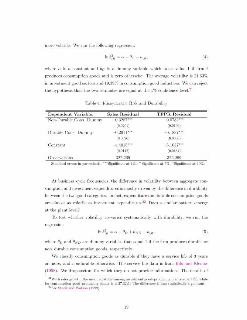
ln ε2ijt = α+ θC + uijt, (4)
where α is a constant and θC is a dummy variable which takes value 1 if firm i
produces consumption goods and is zero otherwise. The average volatility is 21.63%
in investment good sectors and 19.39% in consumption good industries. We can reject
the hypothesis that the two estimates are equal at the 1% confidence level.21
Table 4: Idiosyncratic Risk and Durability
Dependent Variable: Sales Residual TFPR Residual
Non-Durable Cons. Dummy –0.3287∗∗∗ –0.0782∗∗∗
(0.0201) (0.0196)
Durable Cons. Dummy –0.2011∗∗∗ –0.1837∗∗∗
(0.0326) (0.0306)
Constant –4.4015∗∗∗ –5.1037∗∗∗
(0.0142) (0.0134)
Observations 322,269 322,269
Standard errors in parenthesis. ∗∗∗Significant at 1%. ∗∗Significant at 5%. ∗Significant at 10%.
At business–cycle frequencies, the difference in volatility between aggregate con-
sumption and investment expenditures is mostly driven by the difference in durability
between the two good categories. In fact, expenditures on durable consumption goods
are almost as volatile as investment expenditures.22 Does a similar pattern emerge
at the plant level?
To test whether volatility co–varies systematically with durability, we run the
regression
ln ε2ijt = α+ θD + θND + uijt, (5)
where θD and θND are dummy variables that equal 1 if the firm produces durable or
non–durable consumption goods, respectively.
We classify consumption goods as durable if they have a service life of 3 years
or more, and nondurable otherwise. The service life data is from Bils and Klenow
(1998). We drop sectors for which they do not provide information. The details of
21With sales growth, the mean volatility among investment good–producing plants is 32.71%, whilefor consumption good–producing plants it is 27.32%. The difference is also statistically significant.
22See Stock and Watson (1999).
19

the assignment procedure are in Appendix A.4. The regression’s results are reported
in Table 4.
The point estimates suggest that TFPR volatility may actually be greater for
non–durables than for durables. However, once we transform the regression coeffi-
cients to obtain the actual volatility estimates, we find that TFPR volatility is not
statistically different across establishments producing durable and non–durable con-
sumption goods. The bottom line is that we find no evidence in support of the claim
that durability is the reason why investment–good producing plants bear a greater
idiosyncratic risk than plants producing consumption goods.
6 Conclusion
In the recent but fast growing theoretical literature on establishment dynamics, het-
erogeneity in outcomes is often driven by idiosyncratic shocks to technical efficiency,
mark–ups, and input prices. This paper makes some progress towards understanding
the magnitude and cross–sectoral variation of such disturbances.
Using a large panel representative of the entire US manufacturing sector, we found
that idiosyncratic risk accounts for about 80% of the overall uncertainty faced by
plants. We also showed that risk varies greatly across 3–digit sectors, ranging from
6.7% for producers of boot and shoe cut stock, to 35.2% for Primary Smelting and
Refining of Nonferrous Metals.
We propose that the heterogeneity in idiosyncratic risk is driven by the differ-
ential extent to which creative destruction shapes competition across sectors. For-
mal models of Schumpeterian competition imply a positive correlation between the
speed of technological progress, product turnover, and volatility in plant–level out-
comes. We provide evidence in support of these predictions. In particular, our proxy
for idiosyncratic risk is positively associated with measures of product turnover and
investment–specific technological change.
We acknowledge that our evidence is only suggestive. Our conjecture passed a
first test, but establishing causality requires a different methodological approach.
Other factors are likely to contribute to the heterogeneity that we document.
Syverson (2004b) outlines a variety of sectoral characteristics that may be related to
measures of within–sector dispersion in productivity levels. In most models of firm
dynamics, many of those characteristics would also impact the dispersion productivity.
For sure, this is the case for the parameters that drive entry and exit.
20

A Data and Measurement
A.1 Sample Construction
We start by extracting all plants in the ASM panels from 1972 to 1997. For the Census
years, we use the ASM flag variable to select from the Census files the plants belonging
to the ASM panels. To avoid measurement errors from the imputed variables, we
follow most of the economics literature in dropping Administrative Record (AR) files.
We also drop establishments with zero or missing value for employment, or shipments,
or any variable needed for our estimation, such as the total cost of materials, capital
expenditures on buildings or machinery, and production worker hours.
The ASM is a series of five–year panels. In the first years of the panels, the fraction
of plants that can be linked longitudinally to the previous year drop dramatically as
only large, continuing plants ( the so–called certainty cases) are included in adjacent
panels. To avoid measurement issues due to panel rotation, we drop from the sample
all first years of the panels.
When estimating equation (2), we drop plants with less than five observations in
the sample to avoid that mis–measurement of the plant fixed effects propagate to the
residuals. An increase in the cutoff did not change the key results of the paper in any
appreciable way.
When estimating equation (3), we exclude sectors with less than 100 plant–year
observations. This is to guarantee that the results are not driven by a relatively small
number of plants in the sector.
We will make SAS and STATA programs available to researchers with access to
the Census micro data, so that they can replicate the results reported in the paper.
A.2 Variable Definitions
Real Sales. We use the total value of shipments (TVS) deflated by the 4–
digit industry-specific shipments deflator from the NBER manufacturing productiv-
ity database. Although it is possible to adjust total shipments for the change in
inventories, we follow Baily, Bartelsman, and Haltiwanger (2001) and choose to use
the simple measure of gross output. This is to avoid potential measurement issues
associated with imputations of inventories.
Capital. We follow Dunne, Haltiwanger, and Troske (1997) closely in construct-
ing capital stocks. The approach is based on the perpetual inventory method. We
define the initial capital stock as the book value of structures plus equipment, deflated
21

by the BEA’s 2–digit industry capital deflator. In turn, book value is the average of
beginning-of-year and end-of-year assets. The investment series are from the ASM,
deflated with the investment deflators from the NBER manufacturing productivity
database (Bartelsman and Gray, 1996). 2–digit depreciation rates are also obtained
from the BEA.
Labor input. The labor input is measured as the total hours of production and
nonproduction workers. Since the latter are not actually collected, we follow Baily,
Hulten, and Campbell (1992) in assuming that the share of production worker hours
in total hours equals the share of production workers wage payments in the total wage
bill.
Materials. The costs of materials are deflated by the material deflators from the
NBER manufacturing productivity database.
Factor Elasticities. Under constant returns to scale and the usual regularity
conditions, cost minimization implies that each input’s elasticity equals its share in
total production cost. Therefore our ideal estimate of factor elasticity was the industry
average cost share at the finest level of aggregation. Unfortunately capital rental rates,
which are needed to compute capital costs, are only available at the 2–digit level.
Following that route would have introduced a mis–specification error with potentially
large consequences on our residuals’ estimates.
Our solution was to set elasticities for labor and materials equal to their respective
4–digit industry–level revenue shares. The capital elasticity is set equal to the com-
plement to 1, i.e. αkιt = 1− αl
ιt − αmιt . We use the average of revenue shares between
adjacent time periods (i.e., discrete–time approximation to the Divisia index, derived
from the Tornqvist index). This allows factor elasticities to vary over time.
Notice that cost shares and revenue shares coincide only when mark-ups are iden-
tically zero. In any other scenario, mis–specification is still a concern. Our view is
that, however, the resulting bias is substantially lower than in the alternative de-
scribed above.
In calculating labor costs, we follow Bils and Chang (2000) and adjust each 4–digit
industry’s wage and salary payments by a factor that captures all the remaining labor
payments, such as fringe benefits and employer Federal Insurance Contribution Act
(FICA) payments. This factor is based on information from the National Income and
Product Accounts (NIPA), and corresponds to one plus the ratio of the additional
labor payments to wages and salaries at the 2–digit industry level. We apply the same
adjustment factor to all plants within the same 2–digit industry.
22

ASM sample weights. We use the ASM sample weights for all plant–level
regressions, which render the ASM a representative sample of the population of man-
ufacturing plants (Davis, Haltiwanger, and Schuh, 1996).
A.3 Definition of Consumption and Investment Categories
To assign sectors to the consumption and investment categories, we rely on the Bureau
of Economic Analysis’ (BEA) 1992 Benchmark Input–Output Use Summary Table
(before redefinitions) for six–digit transactions. The 1992 Use Table is based on the
1987 SIC system, and thus compatible with the ASM.
The Use Table gives the fraction of output that each three–digit sector supplies
to every other three–digit industry, as well as directly to final demand uses. The final
demand uses correspond to NIPA categories. For each three–digit industry j, we de-
fine its final demand for consumption C(j) as the sum of personal, federal, and state
consumption expenditures. The final demand for investment I(j) is defined analo-
gously. We exclude imports, exports, and inventory changes from our definitions,
since they are not broken down into consumption and investment. Let C and I de-
note the vectors of all the industries’ final consumption and investment expenditures,
respectively.
From the Use Table, we also compute the (square) matrix A of unit input–output
coefficients. This matrix can be easily constructed from the original Use Input–Output
Matrix by normalizing each row by the total commodity column. We can then define
the vectors of all the industries’ total consumption and total investment output by
YC = AYC + C ⇔ YC = (I −A)−1 C
and
YI = AYI + I ⇔ YI = (I −A)−1 I,
respectively. This means that each industry’s consumption goods output also includes
all the intermediate goods whose ultimate destination is final consumption. Similarly,
for investment.
For each three–digit industry j, we compute the share of output destined to con-
sumption, YC(j)/ (YC(j) + YI(j)). We then assign all industries with a share greater
than or equal to 60% to the consumption good sector, and those with a share lower
than or equal to 40% to the investment good sector. We do not assign a consump-
tion/investment good classification to the remaining industries (these industries do
not receive a good classification in the last column of Table 5).
23

We also discard industries whose primary role is supplying intermediate inputs to
other industries. That is, we drop three–digit industries which contribute less than
1% of their total output directly to final consumption and investment expenditures.
A.4 Definition of Durable and Nondurable Consumption Categories
When splitting consumption sectors between durable and nondurable, we follow Bils
and Klenow (1998). Table 2 of their study reports the service life of 57 consumption
good items (those in the Consumer Expenditure Surveys that closely match 4–digit
SIC sectors). Their estimates are either based upon life expectancy tables from in-
surance adjusters, or upon the Bureau of Economic Analysis publication Fixed Re-
producible Tangible Wealth, 1925–1989.
We classify goods as either durable on nondurable, depending on whether their
expected lives are longer or shorter than 3 years. We classify each three–digit sector
as producing durables or nondurables, according to the weighted average of its 4–
digit sub–sectors’ expected lives. Finally, we do not assign a durable/nondurable
consumption classification to three–digit sectors that are not considered in Bils and
Klenow (1998) (these sectors with no service life information are labeled as “Other
Consumption” in last column of Table 5).
B Tables
Table 5: Volatility and Autoregressive Parameter Estimates
SIC TFPR Sales Good Classification
Volatility AR Volatility AR
333 Primary Nonferrous Metals 0.352 0.483 0.404 0.644357 Computer Equipment 0.314 0.548 0.414 0.672 Investment348 Small Arms & Ammo 0.312 0.491 0.429 0.489 Durable Consumption233 Women’s Outerwear 0.295 0.464 0.380 0.599 Other Consumption287 Agricultural Chemicals 0.293 0.420 0.351 0.567 Other Consumption283 Drugs 0.279 0.542 0.273 0.742 Nondurable Consumption241 Logging 0.278 0.422 0.381 0.510385 Ophthalmic Goods 0.273 0.427 0.338 0.561 Durable Consumption281 Industrial Inorganic Chems 0.270 0.411 0.306 0.494 Other Consumption236 Girls’ Outerwear 0.265 0.475 0.345 0.642 Nondurable Consumption393 Musical Instruments 0.264 0.132 0.301 0.115 Durable Consumption232 Men’s Clothing 0.260 0.496 0.343 0.566 Nondurable Consumption238 Misc. Apparel 0.260 0.456 0.348 0.604 Other Consumption231 Men’s Suits & Coats 0.256 0.534 0.353 0.687 Durable Consumption235 Hats & Caps 0.255 0.392 0.294 0.588 Other Consumption367 Elect Components & Acces 0.253 0.554 0.339 0.761277 Greeting Cards 0.252 0.661 0.232 0.682 Other Consumption373 Ship&Boat Build&Repair 0.248 0.375 0.452 0.541
24

Table 5: (continued)
SIC TFPR Sales Good Classification
Volatility AR Volatility AR
311 Leather Finishing 0.248 0.269 0.308 0.455 Other Consumption207 Fats & Oils 0.248 0.312 0.339 0.456 Nondurable Consumption284 Detergents & Cosmetics 0.245 0.432 0.300 0.577 Nondurable Consumption394 Dolls, Toys, & Games 0.242 0.364 0.359 0.577 Durable Consumption376 Guided Missiles, Space Vcl 0.242 0.450 0.358 0.558365 Household Audio-Video Eq 0.241 0.366 0.347 0.646 Durable Consumption209 Misc. Food 0.241 0.486 0.285 0.582 Nondurable Consumption382 Measuring Instruments 0.240 0.390 0.263 0.594 Investment384 Medical Instr & Supplies 0.239 0.455 0.273 0.649381 Navigation Equipment 0.236 0.372 0.305 0.515 Investment366 Communication Equipment 0.236 0.441 0.329 0.610 Investment242 Sawmills & Planing Mills 0.235 0.304 0.331 0.592324 Cement, Hydraulic 0.235 0.579 0.263 0.629 Investment374 Railroad Equipment 0.235 0.267 0.537 0.311 Investment321 Flat Glass 0.234 0.210 0.315 0.221 Other Consumption234 Women’s Underwear 0.232 0.525 0.294 0.705 Nondurable Consumption214 Tobacco Stemming 0.232 0.339 0.417 0.744 Other Consumption295 Asphalt Paving & Roofing 0.230 0.295 0.410 0.447326 Pottery & Related Prods 0.230 0.446 0.297 0.515359 Industrial Machinery 0.230 0.330 0.326 0.616317 Handbags 0.230 0.550 0.337 0.802 Other Consumption386 Photo Equip and Supplies 0.228 0.517 0.268 0.580329 Misc Nonmetal Mineral Prod 0.227 0.480 0.292 0.650259 Misc. Furniture 0.227 0.302 0.295 0.647 Investment286 Organic Chemicals 0.224 0.457 0.294 0.560 Other Consumption208 Beverages 0.221 0.518 0.257 0.582 Nondurable Consumption344 Metal Products 0.220 0.393 0.358 0.523 Investment354 Metalworking Machinery 0.218 0.400 0.300 0.516 Investment399 Misc Manufactures 0.216 0.100 0.331 0.196225 Knitting Mills 0.215 0.460 0.342 0.595 Nondurable Consumption226 Dyeing Textiles 0.215 0.602 0.324 0.692 Other Consumption372 Aircraft and Parts 0.214 0.498 0.263 0.581203 Canned Fruits & Vegtbls 0.212 0.458 0.296 0.588 Nondurable Consumption339 Misc Primary Metal Prods 0.212 0.529 0.282 0.603369 Electrical Equipment 0.210 0.443 0.306 0.591 Other Consumption353 Construction & Mining 0.208 0.492 0.376 0.583 Investment206 Sugar 0.207 0.356 0.272 0.604 Nondurable Consumption363 Households Appliances 0.207 0.501 0.343 0.625 Durable Consumption289 Misc. Chemicals 0.205 0.479 0.262 0.588 Other Consumption327 Concrete & Plaster 0.204 0.414 0.308 0.574 Investment252 Office Furniture 0.204 0.313 0.264 0.559 Investment314 Footwear 0.203 0.539 0.328 0.639 Nondurable Consumption391 Jewelry & Silverware 0.201 0.528 0.283 0.713 Durable Consumption279 Services for Printing 0.201 0.418 0.238 0.759 Other Consumption325 Clay Products 0.199 0.477 0.265 0.545 Investment352 Farm Machinery 0.198 0.374 0.350 0.466 Investment355 Special Industry Machinery 0.198 0.366 0.298 0.561 Investment239 Misc. Textiles 0.197 0.474 0.313 0.744 Other Consumption347 Metal Services 0.196 0.344 0.253 0.663356 General Industry Machinery 0.194 0.417 0.270 0.551 Investment274 Misc. Publishing 0.193 0.499 0.188 0.708 Durable Consumption229 Misc. Textile Goods 0.193 0.481 0.275 0.664 Other Consumption
25

Table 5: (continued)
SIC TFPR Sales Good Classification
Volatility AR Volatility AR
364 Elec. Lighting and Wiring 0.193 0.490 0.263 0.610362 Electrical Apparatus 0.193 0.441 0.268 0.639 Investment396 Buttons & Needles 0.192 0.482 0.374 0.726 Other Consumption308 Misc. Plastic Prods 0.191 0.403 0.279 0.568 Other Consumption351 Engines & Turbines 0.191 0.502 0.294 0.582379 Misc. Transportation 0.189 0.371 0.401 0.605 Durable Consumption205 Bakery Products 0.188 0.403 0.222 0.655 Nondurable Consumption272 Periodicals: Publishing 0.188 0.597 0.157 0.696 Nondurable Consumption254 Shelving & Lockers 0.188 0.465 0.289 0.617 Investment361 Electr. Distrib. Equipment 0.187 0.525 0.265 0.710 Investment243 Millwork 0.186 0.447 0.281 0.590 Investment387 Watches, Clocks 0.185 0.383 0.333 0.839 Durable Consumption332 Iron & Steel Foundries 0.185 0.629 0.303 0.719345 Screw Machine Prods, Bolts 0.184 0.442 0.245 0.677282 Plastic Materials 0.183 0.455 0.261 0.559 Other Consumption336 Nonferrous Foundries 0.183 0.460 0.263 0.676334 Secondary Nonferrous Mat 0.182 0.357 0.389 0.596371 Motor Vehicles and Equip 0.181 0.361 0.326 0.474349 Misc Fabricated Metal Prod 0.181 0.481 0.266 0.609316 Luggage 0.180 0.398 0.232 0.613 Durable Consumption301 Tires 0.180 0.440 0.266 0.516 Nondurable Consumption358 Refrigeration Machinery 0.180 0.392 0.287 0.551 Investment299 Misc. Petroleum 0.179 0.531 0.272 0.621 Nondurable Consumption261 Pulp Mills 0.179 0.338 0.226 0.349 Other Consumption335 Nonferrous Rolling & Draw 0.179 0.504 0.295 0.611204 Grain Mill Products 0.178 0.289 0.264 0.474 Nondurable Consumption273 Books 0.177 0.595 0.181 0.696 Durable Consumption331 Blast Furnace & Steel Prd 0.176 0.396 0.275 0.459278 Bookbinding 0.176 0.495 0.207 0.755 Other Consumption221 Cotton Fabric 0.175 0.328 0.263 0.663 Other Consumption212 Cigars 0.175 0.657 0.259 0.771 Nondurable Consumption302 Rubber Footwear 0.175 0.530 0.303 0.698 Other Consumption201 Meat Products 0.174 0.351 0.268 0.614 Nondurable Consumption202 Dairy Products 0.172 0.364 0.240 0.576 Nondurable Consumption343 Heating Equipment 0.171 0.546 0.271 0.694 Investment342 Cutlery 0.170 0.471 0.224 0.671 Other Consumption249 Misc. Wood Products 0.169 0.408 0.244 0.543 Other Consumption227 Carpets & Rugs 0.169 0.512 0.283 0.715 Durable Consumption213 Chewing Tobacco 0.168 0.535 0.153 0.786 Nondurable Consumption306 Rubber Products 0.168 0.472 0.249 0.553 Other Consumption223 Wool Fabric 0.167 0.586 0.243 0.594 Other Consumption322 Glass & Glassware 0.167 0.534 0.235 0.784 Durable Consumption346 Metal Forging 0.166 0.396 0.274 0.717 Other Consumption305 Packing Devices 0.166 0.321 0.227 0.391 Other Consumption341 Metal Cans 0.166 0.361 0.285 0.496 Other Consumption275 Commercial Printing 0.166 0.299 0.207 0.596 Other Consumption285 Paints 0.164 0.600 0.240 0.709395 Pens & Pencils 0.164 0.408 0.206 0.544 Other Consumption323 Glass Products 0.164 0.370 0.234 0.602 Other Consumption263 Paperboard Mills 0.163 0.446 0.192 0.437 Other Consumption251 Household Furniture 0.159 0.469 0.251 0.769 Durable Consumption228 Yarn & Thread Mills 0.157 0.431 0.311 0.635 Other Consumption
26

Table 5: (continued)
SIC TFPR Sales Good Classification
Volatility AR Volatility AR
222 Silk Fabric 0.155 0.491 0.244 0.693 Other Consumption224 Narrow Fabric 0.154 0.383 0.252 0.779 Other Consumption262 Paper Mills 0.153 0.463 0.197 0.571 Other Consumption244 Wood Containers 0.152 0.309 0.287 0.662 Other Consumption291 Petroleum Refining 0.151 0.377 0.247 0.582 Nondurable Consumption267 Converted Paper Prods 0.151 0.509 0.211 0.678 Other Consumption271 Newspapers: Publishing 0.149 0.409 0.158 0.312 Nondurable Consumption245 Wood Buildings 0.147 0.379 0.360 0.610 Investment319 Other Leather Goods 0.141 0.331 0.206 0.746 Other Consumption328 Stone Products 0.137 0.567 0.182 0.515 Investment253 Public Bldg Furniture 0.133 0.515 0.258 0.601315 Leather Gloves 0.132 0.459 0.210 0.331 Other Consumption276 Business Forms 0.122 0.377 0.146 0.744 Other Consumption265 Paperboard Containers 0.115 0.526 0.187 0.626 Other Consumption375 Motorcycles, Bicycles 0.088 0.184 0.323 0.871 Durable Consumption313 Boot & Shoe Cut Stock 0.067 0.712 0.113 0.496 Other Consumption
27

Table 6: 1987 SIC
SIC Description
20 Food and Kindred Products21 Tobacco Products22 Textile Mill Products23 Apparel24 Lumber and Wood Products25 Furniture26 Paper Products27 Printing and Publishing28 Chemicals29 Petroleum Refining30 Rubber and Miscellaneous Plastics Products31 Leather and Leather Products32 Stone, Clay, Glass, and Concrete Products33 Primary Metal Industries34 Fabricated Metal Products, except Machinery and Transportation Equipment35 Industrial and Commercial Machinery and Computer Equipment36 Electronic and Other Electrical Equipment, except Computer Equipment38 Instruments and Related Products39 Miscellaneous Manufacturing Industries
References
Abraham, A., and K. White (2006): “The Dynamics of Plant–Level Productivity
in US Manufacturing,” Census Bureau Working Paper #06-20.
Aghion, P., N. Bloom, R. Bludell, R. Griffith, and P. Howitt (2005):
“Competition and Innovation: An Inverted-U Relationship,” Quarterly Journal of
Economics, 120(2), 701–728.
Aghion, P., C. Harris, P. Howitt, and J. Vickers (2001): “Competition, Im-
itation, and Growth with Step–by–Step Innovation,” Review of Economic Studies,
68, 467–492.
Aghion, P., and P. Howitt (1992): “A Model of Growth through Creative De-
struction,” Econometrica, 60, 323–51.
28

Bachman, R., and C. Bayer (2013): “Wait–and–see Business Cycles?,” Journal of
Monetary Economics, Forthcoming.
Baily, M. N., E. J. Bartelsman, and J. Haltiwanger (2001): “Labor Produc-
tivity: Structural Change And Cyclical Dynamics,” The Review of Economics and
Statistics, 83(3), 420–433.
Baily, M. N., C. Hulten, and D. Campbell (1992): “Productivity Dynamics in
Manufacturing Plants,” Brooking Papers on Economic Activity: Microeconomics,
4(1), 187–267.
Bartelsman, E., and P. Dhrymes (1998): “Productivity Dynamics: US Manufac-
turing Plants, 1972–1986,” Journal of Productivity Analysis, 9, 5–34.
Bartelsman, E., and M. Doms (2000): “Understanding Productivity: Lessons
from Longitudinal Microdata,” Journal of Economic Literature, 38, 569–594.
Bartelsman, E. J., and W. Gray (1996): “The NBER Manufacturing Produc-
tivity Database,” NBER Technical Working Papers 0205, National Bureau of Eco-
nomic Research, Inc.
Bils, M., and Y. Chang (2000): “Understanding how price responds to costs and
production,” Carnegie-Rochester Conference Series on Public Policy, 52(1), 33–77.
Bils, M., and P. J. Klenow (1998): “Using Consumer Theory to Test Competing
Business Cycle Models,” Journal of Political Economy, 106(2), 233–261.
(2004): “Some Evidence on the Importance of Sticky Prices,” Journal of
Political Economy, 112(5), 947–985.
Caggese, A. (2012): “Entrepreneurial Risk, Investment, and Innovation,” Journal
of Financial Economics, 106(2), 287–307.
Campbell, J. Y., M. Lettau, B. G. Malkiel, and Y. Xu (2001): “Have Indi-
vidual Stocks Become More Volatile? An Empirical Exploration of Idiosyncratic
Risk,” Journal of Finance, 56(1), 1–43.
Castro, R., G. L. Clementi, and G. MacDonald (2004): “Investor Protec-
tion, Optimal Incentives, and Economic Growth,” Quarterly Journal of Economics,
119(3), 1131–1175.
29

(2009): “Legal Institutions, Sectoral Heterogeneity, and Economic Develop-
ment,” Review of Economic Studies, 76(2), 529–561.
Chang, Y., and J. Hong (2006): “Do Technological Improvements in the Manufac-
turing Sector Raise or Lower Employment?,” American Economic Review, 96(1),
252–368.
Chun, H., J.-W. Kim, R. Mork, and B. Yeung (2008): “Creative Destruction
and Firm–Specific Performance Heteroeneity,” Journal of Financial Economics, 89,
109–135.
Clementi, G. L., and T. Cooley (2009): “Executive Compensation: Facts,”
NBER Working Paper # 15426.
Clementi, G. L., and H. A. Hopenhayn (2006): “A Theory of Financing Con-
straints and Firm Dynamics,” The Quarterly Journal of Economics, 121(1), 229–
265.
Clementi, G. L., and D. Palazzo (2013): “Entry, Exit, Firm Dynamics, and
Aggregate Fluctuations,” Working Paper, NYU Stern.
Copeland, A., and A. Shapiro (2013): “Price Setting in an Innovative Market,”
Federal Reserve Bank of New York.
Cunat, A., and M. J. Melitz (2010): “Volatility, Labor Market Flexibility, and
the Pattern of Comparative Advantage,” Journal of the European Economic Asso-
ciation, forthcoming.
Cummins, J. G., and G. L. Violante (2002): “Investment-Specific Technical
Change in the United States (1947-2000): Measurement and Macroeconomic Con-
sequences,” Review of Economic Dynamics, 5(2), 243–284.
Davis, S., J. Haltiwanger, and S. Schuh (1996): Job Creation and Job Destruc-
tion. MIT Press, Cambridge, MA.
Davis, S. J., and J. Haltiwanger (1992): “Gross Job Creation, Gross Job De-
struction, and Employment Reallocation,” Quarterly Journal of Economics, 107(3),
819–863.
Davis, S. J., J. Haltiwanger, R. Jarmin, and J. Miranda (2006): “Volatility
and Dispersion in Business Growth Rates: Publicly Traded versus Privately Held
Firms,” NBER Macroeconomics Annual, 21, 107–156.
30

Doraszelski, U., and J. Jaumandreu (2013): “R&D and Productivity: Estimat-
ing Endogenous Productivity,” Review of Economic Studies, Forthcoming.
Dunne, T., J. Haltiwanger, and K. R. Troske (1997): “Technology and jobs:
secular changes and cyclical dynamics,” Carnegie-Rochester Conference Series on
Public Policy, 46(1), 107–178.
Ericson, R., and A. Pakes (1995): “Markov–Perfect Industry Dynamics: A Frame-
work for Empirical Work,” Review of Economic Studies, 62, 53–82.
Evans, D. (1987): “The Relationship between Firm Growth, Size and Age: Estimates
for 100 Manufacturing Firms,” Journal of Industrial Economics, 35, 567–81.
Foster, L., J. Haltiwanger, and C. Krizan (2001): “Aggregate Productivity
Growth: Lessons from Microeconomic Evidence,” in New Developments in Produc-
tivity Analysis, ed. by C. R. Hulten, E. R. Dean, and M. J. Harper, pp. 303–363.
University of Chicago Press.
Foster, L., J. Haltiwanger, and C. Syverson (2008): “Reallocation, Firm
Turnover, and Efficiency: Selection on Productivity or Profitability?,” American
Economic Review, 98(1), 394–425.
Gourio, F. (2008): “Estimating Firm–Level Risk,” Boston University.
Grilliches, Z. (1979): “Issues in assessing the contribution of R&D to productivity
growth,” Bell Journal of Economics, 10(1), 92–116.
Hall, B. (1987): “The Relationship between Firm Size and Firm Growth in the US
Manufacturing Sector,” Journal of Industrial Economics, 35, 583–606.
Herranz, N., S. Krasa, and A. P. Villamil (2009): “Small Firms in the SSBF,”
Annals of Finance, 5, 341–359.
Hopenhayn, H. A. (1992): “Entry, Exit and Firm Dynamics in Long Run Equilib-
rium,” Econometrica, 60, 1127–50.
Khan, A., and J. K. Thomas (2008): “Idiosyncratic Shocks and the Role of Non-
convexities in Plant and Aggregate Investment Dynamics,” Econometrica, 76(2),
395–436.
Lach, S., and R. Rob (1996): “R&D, Investment, and Industry Dynamics,” Journal
of Economics & Management Strategy, 5(2), 217–249.
31
Lee, Y., and T. Mukoyama (2009): “Entry, Exit, and Plant–level Dynamics over
the Business Cycle,” Working paper, University of Virginia.
Michelacci, C., and F. Schivardi (2013): “Does Idiosyncratic Business Risk Mat-
ter For Growth?,” Journal of The European Economic Association, 11(2), 343–368.
Quadrini, V. (2003): “Investment and Liquidation in Renegotian–Proof Contracts
with Moral Hazard,” Journal of Monetary Economics, 51, 713–751.
Samaniego, R. (2009): “Entry, Exit and Investment–Specific Technical Change,”
American Economic Review, 100(1), 164–192.
Stock, J. H., and M. W. Watson (1999): “Business cycle fluctuations in US
macroeconomic time series,” in Handbook of Macroeconomics, ed. by J. B. Taylor,
and M. Woodford, vol. I, chap. 1, pp. 3–64. Elsevier Science B.V.
Syverson, C. (2004a): “Market Structure and Productivity: A Concrete Example,”
Journal of Political Economy, 112(6), 1181–1222.
(2004b): “Product Substitutability and Productivity Dispersion,” Review of
Economics and Statistics, 86(2), 534–550.
(2011): “What Determines Productivity?,” Journal of Economic Literature,
49(2), 326–365.
32